HybMT: Hybrid Meta-Predictor based ML Algorithm for Fast Test Vector Generation

ML models are increasingly being used to increase the test coverage and decrease the overall testing time. This field is still in its nascent stage and up till now there were no algorithms that could match or outperform commercial tools in terms of speed and accuracy for large circuits. We propose an ATPG algorithm HybMT in this paper that finally breaks this barrier. Like sister methods, we augment the classical PODEM algorithm that uses recursive backtracking. We design a custom 2-level predictor that predicts the input net of a logic gate whose value needs to be set to ensure that the output is a given value (0 or 1). Our predictor chooses the output from among two first-level predictors, where the most effective one is a bespoke neural network and the other is an SVM regressor. As compared to a popular, state-of-the-art commercial ATPG tool, HybMT shows an overall reduction of 56.6% in the CPU time without compromising on the fault coverage for the EPFL benchmark circuits. HybMT also shows a speedup of 126.4% over the best ML-based algorithm while obtaining an equal or better fault coverage for the EPFL benchmark circuits.

I Introduction

Testing VLSI circuits for stuck-at faults is a classical problem in computer science. In its simplest form, the problem is equivalent to the SAT (circuit-satisfiability) problem where we need to find the primary inputs (PIs) that set the value of a certain net to 0 or 1. It is NP-Hard; hence, over the years a lot of heuristics have been developed that ensure good test coverage and also try to minimize testing times as far as possible. This area was considered to be thoroughly established and saturated at least a decade ago.

There are two reasons to look at this area in 2023. The first is that in the last 2-3 years, a few encouraging results have been published that achieve good test coverage with ML-based algorithms [1, 2, 3]. The second is that test-generation times have become very important with the ubiquity of ICs. For instance, Bloomberg reports [4] that a delay of a few days can seriously affect a product’s commercial prospects quite negatively, especially with regards to automotive chips.

ML algorithms in this space are gradually maturing. They still have not moved beyond the 4-decade old ISCAS ’85 benchmarks and no comparisons with commercial tools have been made. We view our work HybMT as a logical successor in this line of work where we answer a simple question, “Is it possible to train a model on the 4-decade old ISCAS ’85 circuits and generate test inputs for recently released benchmark circuits that are up to 70$\times$ larger and simultaneously outperform a popular commercial ATPG tool?” Note that a commercial tool has seen decades of research and meeting its coverage metric or outperforming it in terms of execution time is very challenging. We were successful and achieved a performance gain of 56.6% without sacrificing test coverage. Even if we consider a counterfactual scenario where our tool slightly underperformed vis-a-vis a proprietary tool, we argue that such research is still a significant contribution because such algorithms enrich the open source ecosystem, and others can build on them.

Like other work in this area, we use an optimized version of the PODEM algorithm that is a part of the Fault [5] ATPG tool (part of Google’s OpenLane suite) as the base algorithm. An example of the key decision-making process in PODEM is as follows: if an OR gate’s output is ‘1’, we need to decide which input needs to be set to ‘1’. We design a custom 2-level predictor (or meta-predictor) that makes such predictions, which is known as backtracing. The second-level chooses the output of one of the first-level predictors: SVR regressor and a novel neural network that we propose, HybNN.  

Our specific contributions are as follows: ❶ Modifications to the PODEM algorithm to incorporate ML-based predictions for our no-backtrack probability-based custom heuristic. ❷ Design and implementation of a novel 2-level predictor HybMT based PODEM, which is highly accurate, robust, and much faster than existing state-of-the-art approaches. ❸ Design of a novel meta-predictor that selects the best prediction model for each circuit net at runtime. ❹ Design of a novel neural network HybNN to serve as a backtrace method in PODEM. ❺ Demonstration of significant speedup over a commercial ATPG tool (56.6%) and the existing state-of-the-art ML-based algorithm (126.4%).

Our paper is organized as follows: Section II presents the background of the PODEM algorithm and other key concepts involved in our work. We present the methodology in Section III followed by experiments and results in Section IV. Finally, we present the related work in Section V and conclude in Section VI.

II Background

II-A Path Oriented Decision Making (PODEM)

Path Oriented Decision Making (PODEM) [6] is a fault-oriented deterministic test generation (DTG) algorithm that works by making assignments only at the PIs. PODEM finds the PI values to activate the fault and propagate it to the primary output (PO). To do this, PODEM traverses the circuit till the PI (backtracing) and reverses a previous decision if this decision conflicts with a newer objective (backtracking).

II-B Design for Testability Measures

Controllability/Observability Program (COP): The COP controllability[7] is defined as the probability of setting a net $l$ to logic 1 or 0 by making random PI assignments (each input net has a 50% probability of being 1). Observability is defined as the probability of propagating the value at a net to a primary output (PO).

Sandia Controllability/Observability Analysis Program (SCOAP): The SCOAP [7] combinational controllability is defined as the difficulty of setting a net’s logic level to 1/0. It is represented as CC1/CC0 (resp.). It is the minimum number of PIs required to set the value of net $x$ to a given value $v$. The SCOAP combinational observability is defined as the difficulty of observing the value at an internal net at a PO. It is denoted as CO. It is the minimum number of PI assignments that need to be made to propagate the fault to a PO. Note that SCOAP measures do not take reconvergent fanouts into account.

III Methodology

III-A Implementation Details

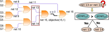
Figure 1: Decision making during backtracing and the use of ‘probability of no-backtrack’ ($p$) as a heuristic

Figure 1 illustrates the decision-making involved during backtracing and the use of no-backtrack probability (p) as a heuristic. Our proposed ATPG algorithm selects the net with a higher value of $p$ (as estimated by HybMT) to avoid wasted work.

III-A1 Input Features of the ML Model

We use the following input features to train our predictors.

The COP Combinational Controllability of a Net $l$ ($CC(l)$): First, we assign the CC values for all the PIs to 0.5 as the PIs need to take the values ‘1’ and ‘0’ randomly. We use the truth tables of different gates to derive the formulae for computing the CC values for the respective output nets of these gates. Then, we calculate the CC values for the intermediate nets and POs of the circuit by traversing the circuit graph in the forward direction.

The COP Combinational Observability of a Net $l$ ($CO(l))$: First, we assign the CO values for all the POs to ‘1’ as any error at the POs is always observable. The formulae for computing the CO values for the input nets of different gates, given the CO values of the output net and CC values of the other input nets, are derived using the truth tables of these gates. Then, we calculate the CO values for the intermediate nets and PIs of the circuit by traversing the circuit graph in the backward direction and using the derived formulae.

The shortest distance of a net from the PIs: The distance feature is normalized to bring the values in the range $[0,1]$ using the following formula

$$distance(l)^{\prime}=\frac{distance(l)-distance_{min}}{distance_{max}-distance_{min}}$$ (1)

where $distance_{min}$ and $distance_{max}$ are the minimum and maximum values for the distance feature computed across all the circuit net samples, respectively.

The type of the gate: The supported gate types are PI, PO, PPI, PPO, NOT, AND, NAND, OR, NOR, XOR, XNOR, DFF, BUF and BAD. The type-of-the-gate feature is represented using 14 bits; we use one-hot encoding. PPI and PPO stand for pseudo-primary inputs and pseudo-primary outputs, respectively, while DFF and BUF stand for D flip-flops and buffers. The gate type BAD represents gates that do not belong to any of the specified gate types.

SCOAP zero controllability (CC0) and SCOAP one controllabillity (CC1): First, we assign the CC0 and CC1 values for all the PIs to 1 and set the depth of each of the logic gates to 1. We compute the sum of the SCOAP controllability values of different input net assignments that justify the desired value at the output net. Then, we take the minimum of these sums and add it to the depth of the gate to get the CC0/CC1 value at the output of the respective logic gate. Finally, we use the CC0 and CC1 values of the logic gate outputs to figure out the CC0 and CC1 values of all the nets by going through the circuit graph in the forward direction.

SCOAP observability (SCOAP CO): First, we assign the CO values for all the POs to 0. Then, we compute the CO value of a logic gate’s input as the sum of the CC0/CC1 values of the other input nets, the CO value of the gate’s output net, and the depth of the gate. The lower the values of the SCOAP measures for a net, the easier it is to control and observe that net.

Fanout of the gate: The fanout of a gate is the number of logic gate inputs driven by the output of the logic gate under consideration.

The input features are shown in Table I. Our lower-level predictors (ML models and HybNN) require the first four features whereas HybMT requires all the eight features.

TABLE I: Input Features of the Predictors

COP controllability	COP observability	Distance from the PI
The type of the gate	SCOAP CCO	SCOAP CC1
SCOAP observability	Fanout of the gate

III-A2 Procedure for Finding Top-$k$ Hard-to-detect Faults in a Circuit

The detection probability ($P_{detect}$) of a fault can be found using Equations (2) and (3). Insight: The detection probability of an s-a-v (stuck at $v$) fault takes into account the probability of setting a value of $\overline{v}$ at the faulty net (fault activation) and the probability of propagating the fault to a PO (given by $CO(l)$).

$$P_{detect}=CC(l)\times CO(l)\text{ for s-a-0 fault at net{ l} }$$ (2)

$$P_{detect}=(1-CC(l))\times CO(l)\text{ for s-a-1 fault at net {l} }$$ (3)

We sort the fault list in an ascending order of the detection probability and thus estimate the top $k$ (hard to detect) faults.

III-A3 Output of the Model

We generated the ground truth label for each circuit net by running PODEM with COP controllability values as a heuristic while backtracing for $k$ hard-to-detect faults of the circuit. During the backtracing procedure of PODEM, if a PI assignment does not lead to any conflict, we label the nets involved in the backtrace as ‘1’, else as ‘0’. A circuit net occurs several times during a single run of PODEM. The input features of a circuit net remain the same across its occurrences, but the ground truth label may keep changing. Hence, we computed the probability of no backtrack $(p)$ for a circuit net $l$ as follows:

$$p=\frac{f(label_{l}=1)}{f_{l}}$$ (4)

Here, $f(label_{l}=1)$ is the frequency of the occurrence of a ‘1’ in the label for the net $l$ and $f_{l}$ is the frequency with which the net $l$ appears in the data. The attributes of the model’s output are mentioned in Table II.

TABLE II: The output of the lower-level predictor (ML model) and its attributes

Output Features	Data Type	Size (in bytes)	Range
Probability of no-backtrack	float	4	[0, 1]

III-B Network Architectures

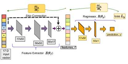
Figure 2: The architecture of the proposed HybNN model with its sub-networks: feature extractor and regressor.

Hybrid Neural Network (HybNN): We designed a novel fully connected feed-forward neural network with a skip connection, which we call HybNN. It has two sub-networks: a feature extractor $E(\theta_{f})$ and a regressor $R(\theta_{f})$. Here, $\theta_{f}$ and $\theta_{y}$ represent the learnable parameters of the respective sub-networks. The feature extractor takes the features of a circuit net as the inputs and performs further extraction to learn the most significant features. We define a linear layer followed by a nonlinear activation function, rectified linear unit (ReLU), as a hidden layer. Every nonlinear layer adds to the complexity and the learning capability of the network. Hence, deeper networks with more hidden layers are found to perform well [8]. $E(\theta_{f})$ has two such hidden layers. We also incorporated a skip connection  [9] that adds the input features directly to the output of $E(\theta_{f})$. The resulting sum is then fed to the function $R(\theta_{y})$. $R(\theta_{y})$ consists of a single hidden layer and an output layer followed by a sigmoid layer. The output of the regressor network is the no-backtrack probability, which is used as the backtracing heuristic. The detailed architecture of HybNN is shown in Fig. 2. The change in the loss function with respect to the model parameters is given by $\partial{L_{y}}/\partial\theta_{y}$ and $\partial{L_{y}}/\partial\theta_{f}$ for the regressor and the feature extractor, respectively. We propagate the gradients backwards as shown in Fig.  2 to train HybNN. With the increase in the number of layers, the gradient becomes very small or zero near the initial layers, and thus the initial layers do not get updated. This is termed as the vanishing gradient problem. A skip connection is used to solve the vanishing gradient problem as it provides an alternate path for the gradient to flow  [9]. We see a significant improvement in performance by adding a skip connection to our neural network.

Hybrid Meta Predictor (HybMT): A meta-predictor model learns to choose among the best predictor models for a given test instance at runtime. We designed a hybrid meta-predictor HybMT that selects between the two best performing lower-level models. The inputs to the HybMT model are the features of a circuit net described in Table I and the output is a class label corresponding to the best-performing model. HybMT is a random forest classifier (RFC) model designed for a binary classification task. An RFC model is based on an ensemble learning technique. It combines the predictions of different decision tree classifiers to give a more accurate prediction than its constituent models. We get the no-backtrack probability $(p)$ for each net from the lower-level model corresponding to the predicted class. Next, we use $p$ to guide the backtracing step in PODEM. The concept of HybMT-based PODEM for the circuit of Fig. 1 is illustrated in Fig. 3.

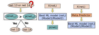
Figure 3: The concept of the HybMT model. $X(net_{i})$ represents the input features of the $i^{th}$ net.

IV Experiments and Results

IV-A Basic Setup

We modified an open-source ATPG framework for PODEM obtained from Fault [5], a part of Google’s OpenLane project [10] to incorporate our changes. We used Flex v2.6.4 and Bison v3.0.4 for parsing the net lists in the ISCAS [11] format. We implemented the ANNs using PyTorch v1.10.2. We conducted experiments to find the optimal learning rate of the Adam optimizer and set it to 0.01. The baseline is a faithful implementation of the ML algorithm described in reference [1]. We have used a standard setup for evaluating our scheme [1]. The same setup including the same set of benchmarks have been used in recent papers in the area.

Data Preparation: Training and test data points must be entirely different (and disjoint) to ensure the correctness and generalizability of the ML models. Hence, we follow a scheme of leave-one-out testing where we keep one benchmark circuit separate for performing inference and train on the remaining benchmark circuits (for every benchmark). We always train our data on the arcane ISCAS 85 [11] benchmark suite, and test on both the ISCAS benchmarks and the much larger and recent EPFL circuits [12].

Cross-Validation: We further divide the training set obtained from the leave-one-out scheme into $k$ equal parts. We keep one of the parts as the validation set, and the other parts constitute the training set. We evaluate the models on the validation set. We repeat this procedure for each data fold. Then, the average accuracy or loss is computed across the $k$-folds. As each of the data points is used for validating the model, the cross-validation score shows the model’s generalization capability. This is the standard practice.

IV-B Lower-level Predictors: Experiments and Results

IV-B1 Traditional ML Models

We started with performing experiments with different regression models: regularized linear regressors (LASSO and Ridge), Support Vector Regressor (SVR), Decision Tree Regressor (DTR) and Random Forest Regressor (RFR) for the no-backtrack probability prediction task. We used 5-fold cross-validation to tune the hyperparameters of these models. The models, their hyperparameters, and the choice of the range of values for tuning are shown in Table III (for the ISCAS suite).

TABLE III: Models for regression with their hyperparameters and ranges for tuning

Models	Hypeparameters	Range
Lasso	Regularization coefficient ($\alpha$)	100 values in the range [0.1,1]
Ridge	Regularization coefficient ($\alpha$)	100 values in the range [0.1,1]
SVR	Regularization coefficient ($C$)	[1e-3, 1e4]
DTR	Depth of the tree	[1,31]
RFR	Number of decision trees	[1,101] in steps of 10

IV-B2 Our Proposed Hybrid Neural Network (HybNN)

The loss function and the optimizer used for training the HybNN model are mean squared error (MSE) and Adam, respectively. We used a uniform distribution in the range $(-\sqrt{k},\sqrt{k})$ to initialize the model weights, where $k=\frac{1}{\text{\#input features}}$.

IV-B3 Execution Times for the Lower-Level Predictors

We ran PODEM on 100 hard-to-detect faults of the ISCAS circuits (results shown in Fig. 4). Let us ignore the results for HybMT (last bar in each cluster) for the time being. We observe that the two best-performing models in terms of their highest geometric mean speedups are HybNN and SVR, respectively. HybNN shows a reduction of 20.4% in CPU time as compared to the baseline, and SVR shows a mean reduction of 1.2%. Out of the 10 benchmarks, HybNN is the best performing model in 8/10 and for the remaining two, SVR is the best.

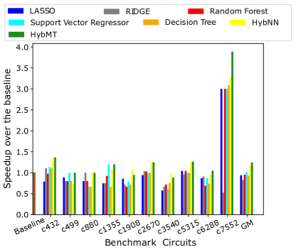
Figure 4: Speedup obtained over the baseline for 100 hard-to-detect faults (ISCAS’85 suite)

Motivation for the HybMT model: These results indicate that there is no unanimous winner among all the ML models that we considered even though HybNN comes close. A hybrid meta-predictor is thus a promising idea as long as it correctly chooses between HybNN and SVR.

IV-C Results with a Commercial ATPG Tool and EPFL Benchmarks

We ran experiments on a commercial ATPG tool for 100 random faults of the EPFL benchmark circuits [12] (arithmetic circuits, up to 70$\times$ larger than ISCAS), and compared them with the baseline and HybMT (results shown in Table IV). Unlike the baseline and HybMT, the commercial tool does not have the notion of hard-to-detect faults; we thus choose 100 random faults (clearly putting ourselves at a disadvantage). Note that we consider the same fault list for both HybMT and baseline. Our HybMT algorithm obtains a speedup of 56.6% over the commercial tool while obtaining the same (or similar) fault coverage. We also performed experiments with the baseline [1] on the EPFL circuits and observed that HybMT has a speed-up of 126.4% over the baseline. In terms of coverage, we are roughly neck-and-neck with the commercial tool. In general, we are better than the commercial tool by roughly 2% (fault coverage). Table V shows a comparison between the number of backtraces and backtracks obtained with HybMT and the baseline for the EPFL circuits. Note that the commercial tool does not report these metrics. We observed that the sum of backtraces and backtracks is proportional to the CPU time. Table V shows that HybMT has a much smaller number of backtraces and backtracks than the baseline for most circuits. This justifies the significant speedup obtained by HybMT.

The radar plot of Fig. 5 shows the importance of each feature in the decision making process of the decision trees of the random forest model (for lower-level predictor selection using HybMT). The greater the importance of a feature, the more it is used in making decisions for the data samples. The $angular$-axis represents the decision trees of the random forest part of the HybMT model, and the $radial$-axis represents the number of times a feature is used to split a decision tree node, weighted by the number of samples it splits. We observed that SCOAP one controllability is the most important feature of all. The results are trying to say that the character of a net is primarily determined by the minimum number of PIs that can control it. Next in importance are the type of the gate and COP observability.

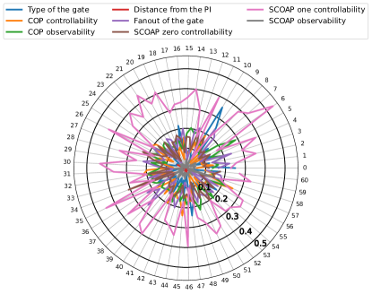
Figure 5: Importance of the features in the decision trees of the RFC meta predictor model

TABLE IV: Comparison with a commercial tool for the EPFL arithmetic benchmark circuits

	CPU Time			Fault Coverage
Benchmark	(in ms)			(in %)
Circuits	Commercial ATPG Tool	Baseline	HybMT	Commercial ATPG Tool	Baseline	HybMT
Adder	190	2,891	180	98	100	100
Barrel-shifter	340	50	55	98	100	100
Divisor	46,480	46,756	46,455	98	97	98
Max	950	44	780	98	100	100
Multiplier	2,510	2,545	2,200	98	100	100
Sine	790	3,25,340	708	97	74	97
Square	1,870	647	800	98	98	98

TABLE V: Comparison with the baseline for the EPFL arithmetic benchmark circuits

Benchmark	Baseline		HybMT
Circuits	#Backtraces	#Backtracks	#Backtraces	#Backtracks
Adder	1,19,809	0	15,723	0
Barrel-shifter	1,064	0	1,078	0
Divisor	1,191,655	4,84,780	1,165,223	3,23,653
Max	1,546	0	2,869	0
Multiplier	27,319	239	21,832	105
Sine	11,347,743	5,653,684	7,853	352
Square	11,880	0	10,850	0

IV-D HybMT: Training and Basic Inference Results (ISCAS ’85)

We generated the ground truth labels for the meta predictor (HybMT) model in two ways. In the first approach, we record the number of times a net is backtracked while running PODEM using different ML model-based probabilities as a heuristic. We take the model that gives the minimum number of backtracks for a net as its class label. Recall that by analyzing the CPU time improvements of the lower-level regressors, we found that HybNN and SVR performed the best for 8 and 2 benchmark circuits, respectively. Hence, in the second approach, we assigned a class label of 0 and 1 to all the nets of the circuits where HybNN and SVR perform the best (resp.).

We obtained better results with the second approach – a coarse-grained approach. The results also corroborate the fact that generating the ground truth labels at the circuit level captures a global view of the circuit’s structure and hence gives better results. The HybMT meta-predictor (top level) achieves an average 5-fold cross-validation accuracy of 99% for the low-level predictor selection task. The results show that our proposed HybMT model reduces the CPU time of PODEM by 26.8% over the baseline for the ISCAS’85 benchmark circuits.

V Related Work

Our primary focus was on recent work (published in the last three years) in the area of ML-based ATPG algorithms that target stuck-at faults. Almost all the highly cited and well regarded work in this field follows the same line of thinking, which is to reduce the number of backtracks in highly optimized versions of PODEM.

In 2020, Roy et al. [7] used the output of ANNs as a backtracing heuristic in PODEM. This was the seminal paper (in recent times). A year later, Roy et al. [1] proposed improvements in the training strategy. In this approach, the backtrace history of a fault is only included in the training data if it decreases the number of backtracks in the ANN-guided PODEM algorithm and the training data is generated by running PODEM on both easy and hard to detect faults of the circuits.

In these works, the ANN used the following input features: distance from the PI (primary input), testability measures and the type of the gate driven by the line. The experiments were performed on 100 hard-to-detect faults of the ISCAS’85 [11] and ITC’99 [7] benchmark circuits. Subsequently, Roy et al. [3] proposed a method based on unsupervised learning to combine different heuristics using principal component (PCA) analysis. The major PCs are used for guiding the backtracing in PODEM. This method also uses the testability measures from SCOAP [7] and the fanout count as the input features. PCA-assisted supervised learning has also been explored in [2] to reduce the complexity of the ANN used for guiding the backtracing in PODEM. So far, no work has presented a robust data generation technique or demonstrated consistent improvement across all benchmark circuits. Thus, they highlight a need for a more robust, accurate and better approach.

In this paper, we compare our work with the latest work in this series that experimentally provided the best results, which is reference [1].

VI Conclusion

The aim of this paper was to reduce the CPU time of the PODEM algorithm as much as possible without sacrificing the fault coverage for the most hard-to-detect faults. Our novel two-level predictor HybMT model based PODEM obtains a speedup of 56.6% over a commercial tool for the EPFL benchmarks. HybMT also outperforms the existing state-of-the-art algorithm [1] by 26.8% and 126.4% for the ISCAS’85 and EPFL benchmarks, respectively. We used the lower-level models to predict the no-backtrack probability $(p)$, and then we used $p$ to guide backtracing in PODEM. We experimented with different traditional ML and neural network models to serve as the lower level models. We found that our novel HybNN model and the support vector regressor (SVR) models perform the best for different benchmark circuits. Our work shows a significant reduction in the CPU time of PODEM while achieving high fault coverage for the ISCAS’85 [11] and EPFL [12] benchmark circuits.

We further conclude that in our work, a global circuit-level view is required to learn better backtracing heuristics. Properly designed neural networks are capable of learning better features and hence are a better candidate for guiding backtracing. The explanations for the meta predictor model indicate that the SCOAP one controllability occurs the maximum number of times in the decision making process of the decision trees of the random forest classifier and hence is the most important feature. Now, our immediate aim is to increase the expressive power of the model by raising the limit of 70$\times$ (test size/train size) to 100$\times$, and look at even larger circuits with sequential elements.

References

- [1] S. Roy, S. K. Millican, and V. D. Agrawal, “Training neural network for machine intelligence in automatic test pattern generator,” in 2021 34th International Conference on VLSI Design and 2021 20th International Conference on Embedded Systems (VLSID). IEEE, 2021, pp. 316–321.
- [2] ——, “Principal component analysis in machine intelligence-based test generation,” in 2021 IEEE Microelectronics Design & Test Symposium (MDTS). IEEE, 2021, pp. 1–6.
- [3] ——, “Unsupervised learning in test generation for digital integrated circuits,” in 2021 IEEE European Test Symposium (ETS). IEEE, 2021, pp. 1–4.
- [4] “How a chip shortage snarled everything from phones to cars,” 2021. [Online]. Available: https://www.bloomberg.com/graphics/2021-semiconductors-chips-shortage/
- [5] M. Abdelatty, M. Gaber, and M. Shalan, “Fault: Open-source eda’s missing dft toolchain,” IEEE Design & Test, vol. 38, no. 2, pp. 45–52, 2021.
- [6] P. Goel, “An implicit enumeration algorithm to generate tests for combinational logic circuits,” IEEE transactions on Computers, vol. 30, no. 03, pp. 215–222, 1981.
- [7] S. Roy, S. K. Millican, and V. D. Agrawal, “Machine intelligence for efficient test pattern generation,” in 2020 IEEE International Test Conference (ITC). IEEE, 2020, pp. 1–5.
- [8] G. F. Montufar, R. Pascanu, K. Cho, and Y. Bengio, “On the number of linear regions of deep neural networks,” Advances in neural information processing systems, vol. 27, 2014.
- [9] K. He, X. Zhang, S. Ren, and J. Sun, “Deep residual learning for image recognition,” in Proceedings of the IEEE conference on computer vision and pattern recognition, 2016, pp. 770–778.
- [10] A. Ghazy and M. Shalan, “Openlane: The open-source digital asic implementation flow,” in Proc. Workshop on Open-Source EDA Technol.(WOSET), 2020.
- [11] F. Brglez, “A neutral netlist of 10 combinatorial benchmark circuits and a target translator in fortran,” in Int. Symposium on Circuits and Systems, Special Session on ATPG and Fault Simulation, June 1985, 1985, pp. 663–698.
- [12] L. Amarú, P.-E. Gaillardon, and G. De Micheli, “The epfl combinational benchmark suite,” in Proceedings of the 24th International Workshop on Logic & Synthesis (IWLS), no. CONF, 2015.