Phase–type representations of stochastic interest rates with applications to life insurance
Abstract.
The purpose of the present paper is to incorporate stochastic interest rates into a matrix–approach to multi–state life insurance, where formulas for reserves, moments of future payments and equivalence premiums can be obtained as explicit formulas in terms of product integrals or matrix exponentials. To this end we consider the Markovian interest model, where the rates are piecewise deterministic (or even constant) in the different states of a Markov jump process, and which is shown to integrate naturally into the matrix framework. The discounting factor then becomes the price of a zero–coupon bond which may or may not be correlated with the biometric insurance process. Another nice feature about the Markovian interest model is that the price of the bond coincides with the survival function of a phase–type distributed random variable. This, in particular, allows for calibrating the Markovian interest rate models using a maximum likelihood approach to observed data (prices) or to theoretical models like e.g. a Vasiček model. Due to the denseness of phase–type distributions, we can approximate the price behaviour of any zero–coupon bond with interest rates bounded from below by choosing the number of possible interest rate values sufficiently large. For observed data models with few data points, lower dimensions will usually suffice, while for theoretical models the dimensionality is only a computational issue.
Keywords: Zero–coupon bond; Phase–type distribution; Stochastic interest rate; Multi-state life insurance; Thiele’s differential equation.
2020 Mathematics Subject Classification: 60J28, 62M05, 91G05, 91G70.
JEL Classification: G22
1. Introduction
This paper considers stochastic interest models, which are state-wise deterministic dependent on an underlying finite state-space Markov process. The spot rate at time is assumed to be on the form
| (1) |
where denotes a time-inhomogeneous Markov jump process on a –dimensional state–space, and , , are deterministic functions. Assuming an arbitrage free bond market, a zero–coupon bond with terminal date can then be defined in terms of its prices by
| (2) |
where is the –algebra generated by . The expectation is taken under some risk–neutral measure (see, e.g., Björk (2009); Elliott and Kopp (1999)). If all , a key result of the paper is that, conditionally on , equals the survival function of an inhomogeneous phase–type distribution.
In the presence of negative interest rates, this is longer certain since may be larger than one and non–monotone. However, assuming that the negative interest rates are bounded from below by a number , we get from (2) that
| (3) |
then equals a survival function of an inhomogeneous phase–type distribution.
The interpretation that the bond prices are (possibly scaled) phase–type survival functions enables us to fit (calibrate) the transition rates of from the observed bond prices by using a maximum likelihood approach. Since phase–type distributions are dense, i.e. can approximate any distribution with a sufficient number of phases, we may then fit a PH to the observed survival function (equivalent to a histogram) such that all observations (bond prices) are hit. The last point of observation may be considered right censored. All fitted transition rates are under a risk–neutral measure .
The functional form of the state–wise price of the bond was noted already in (Norberg, 2003, (3.17)), though its relation to phase–type theory was not mentioned, and its potential was not further explored. We also believe that the “bond price representation” (2) of a phase–type survival function is unknown to the phase–type community.
In the context of multi-state life insurance, modelling stochastic interest rates also play a crucial role. The literature varies from SDE based models, see e.g. Norberg and Møller (1996); Møller and Steffensen (2007); Buchardt (2014); Baños (2020); Asmussen and Steffensen (2020), to the finite state–space Markov chain models of Norberg (1995b, a) on the form (1). In the SDE-based methods, one often relies on an independence assumption between interest rates and biometric risk so that available forward rate curves can be used for valuation; an exception is Buchardt (2014), where dependence between interest rates and biometric risk is incorporated. In either case, the SDE-based models do not integrate into classic Thiele and Hattendorf type of results, which limits time-dynamic valuations based on these traditional methods.
The spot rate model (1), however, can be wholly incorporated into Thiele and Hattendorf type of differential equations for reserves and higher order moments, as shown by Norberg (1995a, b) and further explored in Norberg (2003). These observations allow for dependency between interest rates and transitions in life insurance, as well as time-dynamic valuations, without altering the traditional methods. The latter refers to the model (1) as the Markov chain market while Koller (2012) refers to it as Markovian interest intensities.
In this paper, we work with an extended version of the bond prices,
| (4) |
which in an insurance context are the discounting factors on the event that the terminal state will be . Providing a matrix–representation for (4), we then find how it naturally integrates into the matrix framework of Bladt et al. (2020). The extension is convenient from a mathematical point of view and also relates to the partial (Bladt et al. (2020)) and retrospective reserves in single states ((Norberg, 1991, Sec. 5E)). The treatment of the latter, however, is outside the scope of the current paper. We restate the results of the latter framework in the context of stochastic interest rates. The proofs, and parts of the exposition, will differ from that of Bladt et al. (2020).
Markov jump processes in finance are often used in connection with regime switching models or where the different states are used to alter the parameters of usually SDE-driven processes. Here transitions can take place under some physical measure and may have a real–world interpretation. The Markov chain model for interest rates (1) can be thought of as a regime-switching model under a risk-neutral measure, particularly if the interest rates for each state are known a priori.
The Markov jump process approach can approximate bond price modelling in terms of diffusions. Formal constructions have been made in Bharucha-Reid (1960); Kurtz (1970, 1978); Mijatović and Pistorius (2013). Since phase–type distributions form a dense class of distributions on the positive reals, this paper will offer an alternative and parsimonious way to approximate any zero–coupon bond (arbitrarily close) by a bond on the form (2).
The paper is organised as follows. Section 2 introduces some background and notation. Bond price modelling using phase–type distribution is developed in Section 3. In Section 4, we develop estimation of the Markovian interest rate model, both with and without restricted interest rates, and we provide examples of calibration to diffusion models and real data. In Section 5 we adjust the life–insurance framework of Bladt et al. (2020) to allow for stochastic interest rates of the form (1). It contains examples of how to set up a model using the fitted bond parameters of Section 3 as well as a matrix–based method for calculating the equivalence premium, either via Newton’s method or as an explicit formula. In Section 6 we present a numerical example. For the sake of exposition, the proofs are deferred to Appendix B.
2. Background
2.1. Notation
Unless otherwise stated, row vectors are denoted by bold Greek lowercase letters (e.g., ) and column vectors by bold lowercase Roman letters (e.g., ). Elements of vectors are denoted by the same unbold, indexed letters (like ). The vector is the column vector which is at index and zero otherwise whereas .
Matrices are denoted by bold capital letters (Greek or Roman) and their elements by their corresponding lowercase indexed letters (e.g.). If is a vector (row or column), then denotes the diagonal matrix, which has as diagonal.
2.2. The product integral
Consider a time-inhomogeneous Markov jump process taking values in a finite state space , with intensity matrix (functions) . Denote by the corresponding transition matrix, the elements of which are the transition probabilities for . The transition matrix then satisfies Kolmogorov’s forward and backward differential equations,
| (5) | ||||
The solution to (5), which in general is not explicitly available, will be denoted by
| (6) |
and referred to as the product integral of from to . This is also true for general matrix functions , which satisfy (5) but are not intensity matrices.
Product integrals have several nice properties. For any , it satisfies the product rule
| (7) |
which in turn implies that the product integral is invertible with
| (8) |
If all commute, then
| (9) |
In particular, for , we get
| (10) |
If and commute for all , then
| (11) |
In particular,
| (12) |
where denotes the identity matrix.
Remark 2.1.
The idea behind the notation of the product integral comes from a Riemann type of construction using step–functions. If we approximate by a piecewise constant matrix function taking values on for and where , then by (10) the product integral over equals the matrix exponential
By letting and using (7) we then arrive at the notation (6).
A valuable formula for computing integrals involving product integrals is the so–called Van–Loan’s formula for product integrals (see (Bladt et al., 2020, Lemma 2)), which states that
| (13) |
This formula is valid for matrix functions and , which are piecewise continuous. The matrices and are square matrices of possibly different dimensions, so is not necessarily a square matrix.
Let
where denotes the Kronecker product. The Kronecker product between a matrix and a matrix is defined as the matrix
Using that , we get
and we conclude that
| (14) |
A similar argument gives that
| (15) |
Finally, if and are Riemann integrable matrix functions of dimensions and respectively, then
| (16) |
where denotes the Kronecker sum, defined by , and where the first has the dimension of and the second has the dimension of . To see this, we notice that and commute, so by (11) we get that
For further details on Kronecker products and sums, we refer to Graham (1981)
2.3. Phase–type distributions
Consider a (time–inhomogeneous) Markov jump process , where state is absorbing and are transient. The intensity matrix for is then on the form
| (17) |
where is a sub–intensity matrix consisting of transition rates between transient states, and is a column vector of exit rates, i.e. rates for jumping to the absorbing state. Then by Van-Loan’s formula (13), the transition matrix for is given by
Hence is the matrix which contains the transition probabilities between the transient states from times to .
We assume that , and define . Hence satisfies that , so that is the initial distribution for concentrated on the transient states only. Then
| (18) |
is a row vector that contains the probabilities of the process being in the different transient states at time .
Now let
denote the time until absorption. Then from (18) we immediately get that
| (19) |
since the right-hand side equals the probability of the process belonging to any of the transient states by time , i.e., absorption has not yet occurred. Differentiating (19) and using (5) we see that has a density on the form
| (20) |
Definition 2.2.
The distribution of is called an inhomogeneous phase–type distribution, and we write , where the indexation of is over .
We do not need to specify since it is implicitly given by . Indeed, since row sums of intensity matrices (and hence of (17)) are zero, we have that . If , then we simply write . This corresponds to the underlying Markov jump process being time–homogeneous.
We also notice defines an intensity matrix (without the absorbing state).
The class of phase–type distributions (both PH and IPH) is dense (in the sense of weak convergence) in the class of distributions on the positive reals, implying that any distribution with support may be approximated arbitrarily close by a phase–type distribution. This result is also of considerable practical importance since phase–type distributions can be fitted both to data and distributions using a maximum likelihood approach. For the time–homogenous case, PH, see Asmussen et al. (1996) while for IPH we refer to Albrecher et al. (2022).
3. Phase–type representations of bond prices
Consider the stochastic interest rate model of (1), and let denote the state–space of the Markov jump process with intensity matrix . Let be the column vector which contains the interest rate functions.
The main result of this section is the following result.
Theorem 3.1.
For , let
Then the matrix has the following representation
| (21) |
Proof.
Conditioning on the state of , we get that
so that
| (22) |
In matrix form, this amounts to
| (23) |
Noting that , we hence conclude that (21) holds. ∎
Remark 3.2.
The quantities in Theorem 3.4 are introduced as –deflated transition probabilities in (Buchardt et al., 2020, Appendix 1), where the authors derive the differential equation (23). While they give a martingale–based proof, we provide a probabilistic sample path argument and give a product integral representation.
Remark 3.3.
Assume that all are bounded from below, and let
Then if all interest rates are non–negative, and otherwise provides a lower bound for all of them. Then we have the following result.
Theorem 3.4.
The price of the zero–coupon bond (2) satisfies
| (24) |
Conditional on ,
is the survival function for an IPH distributed random variable, , with initial distribution and intensity matrices , .
In particular, if all interest rates are non–negative, then and the price itself, becomes the survival function.
Proof.
The formula (24) follows directly from the construction of the matrix by summing out over in , which corresponds to post–multiplying by . Next, we notice that
which follows from (12). The matrix is a sub–intensity matrix, which together with the distribution for defines a phase–type representation , (starting at time ). ∎
The forward rate is defined by
Using Theorem 3.4, we may write
where denotes the survival function for . Then
where denotes the density function for . Hence we have proved the following result.
Corollary 3.5.
Conditional on , the forward rate equals the hazard rate at for the random variable , less . i.e.
| (25) |
Another immediate consequence of Theorem 3.4 is the following.
Corollary 3.6.
Assume that all interest rates are non–negative. Then conditional on , the random variable , then has a c.d.f. given by
Proof.
For the case where , the above results are reduced to the following.
Corollary 3.7.
Assume that all interest rates are non–negative. Let and let denote the (initial) distribution of . Then
| (26) | |||||
| (27) | |||||
| (28) |
Remark 3.8.
The density has the interpretation of being the expected present value of the current interest rate accumulated in a small time interval arround , and is the present value of the total accumulated interest rate during .
Example 3.1.
Assume that all interest rates are non–negative. If is time–homogeneous and , then we also have that
where is the expectation of ,
is the stationary distribution of a phase–type renewal process with inter–arrivals being , see (Bladt and Nielsen, 2017, Th. 5.3.4), and . Hence the swap rate can be expressed as
4. Estimation
Time–homogeneous phase–type distributions or inhomogeneous phase–type distribution where the sub–intensity matrices are on the form
for some parametric function , can be estimated in terms of an EM algorithm.
An observation from a phase–type distribution is hence considered to be the time until a Markov jump process is absorbed, where all transitions and sojourn times in the different states are unobserved. This makes the estimation an incomplete data problem, which an EM algorithm can solve. Essentially the unobserved sufficient statistics (number of jumps between states, total time in then different states) are replaced by their conditional expectations given data and used in the explicit formulas for the maximum likelihood estimators. This updates the parameters, and the procedure is repeated until convergence. Convergence is secured as the likelihood increases in each step. The limit may be a global or only a local maximum.
Repeated data (absorption times), of course result in the same conditional expectations given their data. This carries over to weighted data as well, and hence the EM algorithm may efficiently estimate data in histograms. In particular, we may estimate to theoretical distributions by treating their discretised density as a histogram. This provides the link to fitting the intensity matrix of in (1) through bond prices, (2) or (3), either in terms of observed data or to a theoretical model.
Indeed, consider bond prices available at different maturities . Then according to Theorem 3.4 we have that
for some and where . Then must satisfy that
This can be achieved by choosing
In the life–insurance context in Denmark, by regulation the bond prices (discounting factors) must be computed from discrete forward rates, , published by the Danish Financial Supervisory Authority. Thus
from which
Hence
| (29) |
Hence calibrating to data , can be done by fitting PH or IPH distributions to using an EM algorithm. The possible interest rates can either be picked by the EM algorithm (referred to as unrestricted interest rates), or we can fix the possible rates to values (or functions) of our choice (restricted interest rates).
In the former case, we obtain a maximum likelihood estimate for the parameters. The estimate for is then readily obtained from
To find the induced interest rates, we also have from Theorem 3.4 that
so we conclude that the estimated exit rates must satisfy
where is the vector of ones. Hence the induced interest rates are given by
Neither the transition rates nor the interest rates are unique, but the resulting discount factor (bond price) is invariant under different representations, which is all that matters regarding reserving in the insurance context.
If, in turn, we decide to choose the possible range of interest rates ourselves, then the EM–algorithm is modified not to update the exit rates. This modification is easily dealt with by simply removing updates of the latter in the original EM algorithm of Asmussen et al. (1996) or Albrecher et al. (2022). See Appendix A for details. In this case, the exit rates will be fixed at
so
While the parametrisation of the transition rates may not be unique, the interest rates remain fixed.
We now present two examples of fitting to real data and one example to a theoretical model. The estimation is computed using the R–package matrixdist.
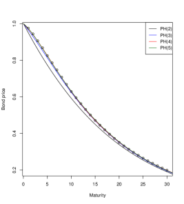
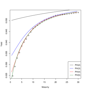
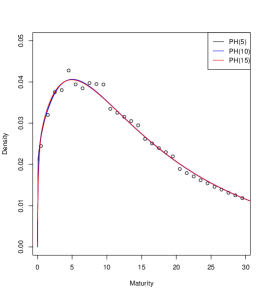
Example 4.1 (Fitting to observed bond prices with restricted interest rates).
Bond prices, as of 31/12/2003 (time zero) with maturities years are available from the Danish Financial Supervisory Authority and given by 0.9755051, 0.9434934, 0.9059545, 0.8679149, 0.8251354, 0.7857250, 0.7472528, 0.7075066, 0.6679984, 0.6286035, 0.5951316, 0.5625969, 0.5310441, 0.5005108, 0.4710280, 0.4448469, 0.4197550, 0.3958013, 0.3728296, 0.3508858, 0.3319907, 0.3140894, 0.2970098, 0.2808430, 0.2654229, 0.2508400, 0.2369349, 0.2237965, 0.2112725, 0.1994495, respectively.
This corresponds to an empirical survival distribution to which we can then fit phase–type distributions of different dimensions. Regarding the discretisation, we let , denote the data points with probability mass , where , and a right censored data point at 30 with probability mass . Since all observed bond prices are less than one, we have , corresponding to an environment with non-negative interest rates.
We used and phases, with state–wise interest rates being , for the different dimensions . Underlying this choice is the assumption that the interest rates fluctuate between and , and the ’s are obtained as the points that divide the interval into , including the right endpoint. The vectors will serve as exit rate vectors of the phase–type distributions to be fitted.
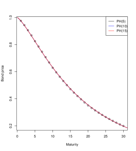
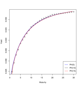
In Figure 1 (left), we have plotted the phase–type fits to the empirical survival curve for dimensions . At dimension 3, we obtain a decent fit and excellent fits for dimensions 4 and 5. The likelihood values for 4 cases are -3.178171, -3.16838,-3.166633, and -3.166182. Further experimentation with dimensions 10 and 15 resulted in likelihoods of -3.165002 and -3.164654, respectively. However, the plots of bond prices and yields are indistinguishable from the plots corresponding to dimension 5, see Figure 2. We can also assess the quality of the fits by plotting the estimated density function vs. the weighted data, shown in Figure 3. Again the plots for dimensions are almost indistinguishable. Therefore, we conclude that dimension 4 or 5 will suffice to approximate the bond prices.
The estimates of the sub–intensity matrix (under a risk neutral measure ) for dimensions are given by
To fit the bond prices, the initial distributions of Markov processes were all on the form of appropriate dimension, i.e., initiation in state 1.

Example 4.2 (Fitting to 2019 bond prices with unrestricted interest rates).
To illustrate the applicability of our methods also in the case of a negative interest rate environment, we can instead fit to bond prices as of 31/12/2019 from the Danish Financial Supervisory Authority; this dataset consists of maturities of years. In this case, we let the EM algorithm choose the necessary positive and negative interest rates.
The first five years have bond prices above one and given by 1.00231736, 1.00403337, 1.00445679, 1.00382807, and 1.00197787, which reflects the (slightly) negative interest rate environment at the time. From (29), we get as the exponential factor to down-scale prices to below one.
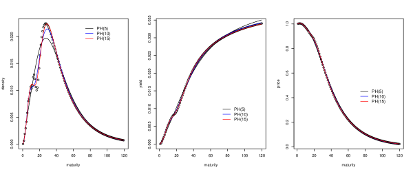
In Figure 5, we show the phase–type fits to the bond prices. We have used the subclass of time–homogeneous Coxian distributions, where initiation is always in state 1, and the only possible transitions are from a state, say, to the following, , or to exit to the absorbing state.
If the primary purpose is using the fits as a discounting factor in a life–insurance model, then probably all fits could be used (right plot). If the yield curve fitting is the concern, then only dimensions 10 and 15 seem to catch the appropriate curvature. Regarding the probability density of the phase–type, the 15-dimensional fit is the best.
To exemplify, we consider the ten dimensional fit. The fitted intensity matrix, , for , is given by
The matrix contains six different parameter values. The matrix structure is carried over from the phase–type fit to the (discounted) bond prices. The blocks with the same parameters correspond to Erlang blocks, i.e. convolution of exponential distributions with the same parameter.
The induced (estimated) interest rates (in ) are, respectively,
These should also be counted as parameters.
Example 4.3 (Fitting to a two–factor Vasicek model).
In this example we consider the two–factor Vasicek short rate model G2++ (see Brigo and Mercurio (2006)) with an initial negative interest rate.
Here the bond prices as of time zero are given by
where
We chose the same parameters as in Diez and Korn (2020), Fig. 3, apart from the initial interest rate , which was set to . Hence the parameters are
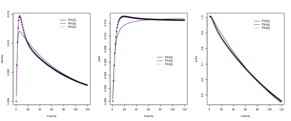
We fitted 3,4 and 5 dimensional time–homogeneous phase–type distributions with a Coxian structure to the discounted bond prices . Here and the intensity matrix for based on 4 phases is given by
with corresponding interest rates , while for 5 phases, we get
The corresponding (estimated) interest rates are . A total of six parameters specify the four-dimensional model, while seven parameters determine the five-dimensional.
5. Applications to life insurance
In this section, we incorporate the stochastic interest rate model of the previous sections to life insurance valuations. We consider the model introduced by Norberg (1995a, b) and extend their results on reserves and higher order moments to so-called partial reserves and higher order moments, that is, corresponding results on events of the terminal state. Partial reserves and moments play important roles when dealing with so-called retrospective reserves in single states (cf. [5, Section 5.E]), which, however is outside the scope of the present paper. We provide this extension following the matrix approach of Bladt et al. (2020) so that these types of results are extended to allow for stochastic interest rates on the form (1). The extensions of the results of these papers are pointed out in a series of remarks throughout the section.
5.1. A Life insurance model with stochastic interest rates
Let be a time–inhomogeneous Markov jump process with a finite state–space and intensity matrix . Then we define a payment process by
| (30) |
where are continuous payment rates (negative if premiums) and lump sum payments, which occur according to the counting measure . The intensity matrix is decomposed into
| (31) |
where is a non–negative matrix and, consequently, a sub–intensity matrix, i.e. row sums are non–positive. The counting process is linked to the transitions of in the following way. Upon transition from to , , in at time , a lump sum payment of will be triggered with probability
| (32) |
If , then denotes an inhomogeneous Poisson process with intensity , and a lump sum during a sojourn in state will then be triggered in with probability .
Finally, we assume that the spot interest rates in state follow a deterministic function . Hence the interest rates follow the model (1).
Remark 5.1.
The classic Markov chain life insurance setting of, e.g., Hoem (1969); Norberg (1991), is the recovered if , and if the probabilities (32) are either zero or one. Extending the classic setting to allow for different interest rates in the different states was considered in Norberg (1995a, b), where Thiele type of differential equations for the reserves and higher order moments were derived.
For the purpose of computing reserves and higher order moments, (Bladt et al., 2020, (3.8)–(3.11)), we let denote the vector containing the continuous rates, and define matrices
where denotes the diagonal matrix with as diagonal. The operator denotes Schur (entrywise) matrix product, defined by for matrices and .
Hence is the matrix containing the lump payments at transitions and at Poisson arrivals during sojourns, is the matrix whose ’th element is the expected reward accumulated during upon transition from to , or during a sojourn in state if . The matrix is more technical to be used when dealing with higher order moments.
Finally, we let
denote the vector of interest rates.
Now assume that the interest rate process is modelled and fitted using bond prices like in Section 3. Accordingly there is a Markov jump process with state–space and intensity matrix , say, such that the corresponding bond prices are given as in Theorem 3.4. Similarly, we let denote the Markov jump process governing the transition between the biometric states with the state–space and intensity matrix . Hence the Markov jump process appearing in (30) can be written on the form
| (33) |
with state–space .
Hence we need to decide upon an ordering of , which will be lexicographical. This means the for elements ,
In other words, each biometric state consists of sub–states depending on the state of the underlying Markov process , see Figure 6.
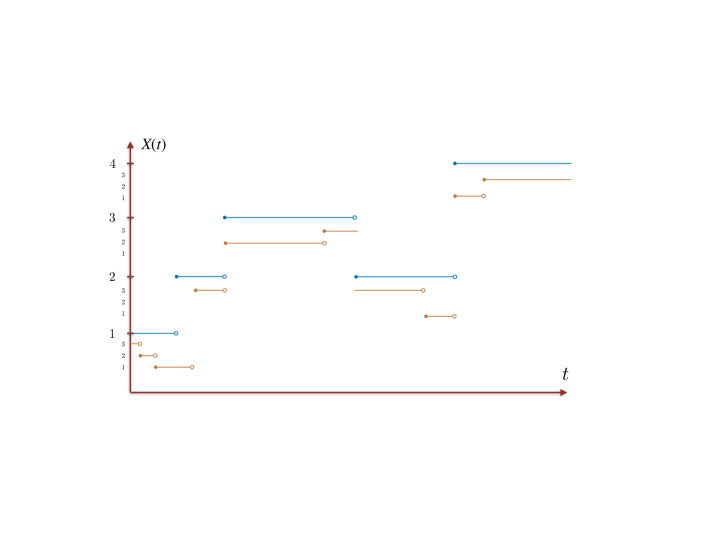
The processes and may or may not be independent, and the payment processes (30) likewise may or may not be independent of . In the independent case the processes and are defined on each their state–space, and the common state–space will be the product set of the two. If the processes are sharing states, with the possibility of having simultaneous jumps, then we obtain dependency of the processes. Such a case could, e.g. be a rise in the interest rate causing an increased intensity of jumping to surrender or free–policy states (see, e.g., Buchardt (2014)).
In the following example, we consider the simplifications in the representations when assuming independence.
Example 5.1 (Independence).
If the transition rates of satisfy, for all , , and , ,
we have that and are independent. Using the lexicographical ordering, we can, in this case, obtain compact matrix representations in terms of the two processes as follows. The transition intensity matrix of is now of the form
where denotes the Kronecker sum, and where denotes the identity matrix of dimension . We recall that the Kronecker product, , is defined by , where .
The interest rate vector satisfies
where .
If we further assume that the payment process (30) is independent of , i.e. such that the payment functions satisfy, for all and ,
we have that the payment matrices are on the form
where
Similarly, we may directly decompose :
such that the decomposition (31) reads
The conceptual difference in the decomposition of and lies in the absence of lump sum payments upon transition between interest levels.
5.2. Reserves
We now consider the valuation of the payment process . Introduce the matrix of partial state–wise prospective reserves,
Due to the stochastic interest rates, this is an extension of Bladt et al. (2020). With , introduced in (21), modified to the setup of this section as
we have the following result.
Theorem 5.2.
The matrix of partial state-wise prospective reserves has the following integral representation:
| (34) |
Proof.
See Appendix B. ∎
The actual computation of the reserves can be effectively executed using the following Van–Loan type of formula, which avoids integration.
Corollary 5.3.
can be extracted from the relation
Finally, we state and prove Thiele’s differential equations for partial reserves with stochastic interest rates.
Theorem 5.4 (Thiele).
where . For the conventional state–wise prospective reserves, , this has the form
where .
Proof.
See Appendix B. ∎
Remark 5.5.
Writing out the elements of the differential equation for , we get for ,
which is the differential equation obtained in (Norberg, 1995a, (3.2)) in the case of a first-order moment.
5.3. Higher order moments
Consider the matrix of partial state-wise higher order moments of future payments, given by, for (see (Bladt et al., 2020, (3.6)-(3.7))),
and introduce what we shall term the reduced partial state-wise higher order moments:
Since all payment functions and transition rates are deterministic, results for these higher-order moments are now straightforward to obtain by using the undiscounted result,
where , , contains the partial state-wise ’th moment, normalised by , of the undiscounted future payments (see (Bladt et al., 2020, (7.4))), i.e. with no interest rate. Indeed, rates and lump sums must be replaced by the discounted versions with discounting factor, (for fixed ). Powers of lumps sums like , , are discounted by . Denoting
we then obtain the following version of Hattendorff’s theorem for partial reserves with stochastic interest rate.
Theorem 5.6.
The matrix of reduced partial state-wise higher order moments satisfies the integral equation, for ,
Proof.
See Appendix B. ∎
Defining
we get by Van Loan that
| (35) |
From these results, we can derive a number of classical results. Differentiation of (35) gives
We then obtain the following differential equation by only considering the first row times the last column.
Theorem 5.7.
The matrix of reduced partial state-wise higher order moments satisfies the system of differential equations, for ,
with terminal condition .
Remark 5.8.
A martingal-based proof for the corresponding (unreduced) state-wise moments, , can be found in Norberg (1995a).
Example 5.2 (Independence continued).
We can continue our decompositions from the independence case of Example 5.1 to reserves and higher-order moments. Indeed, since
we get from (16) that
Thus, each diagonal block element can be computed using these representations when setting up the matrix for the computation of these higher order moments.
In particular, for partial state-wise reserves (i.e. ), we obtain a more direct expression. Assuming that the initial biometric state is , the terminal and that the initial distribution of the fitted interest rate phase–type distribution is . Then
which is consistent with similar expressions obtained in Norberg (1995b).
5.4. Equivalence premium
Assume that such that is a parameter of either and/or only. Hence, could, e.g., be a premium rate in state or a transition payment between some states. We then write so that
If the interest rates satisfy , then is a sub–intensity matrix, so that is a sub–probability matrix, i.e.
If is continuously differentiable and and are continuous, then by Leibniz’ integral rule
Hence we get from the Van Loan formula (13),
| (39) |
Remark 5.9.
If state is the starting state, we can formulate the equivalence principle by finding the that solves
using Newton’s method,
where denotes the partial derivative wrt. . For example, if is a constant premium (rate) such that
i.e. a matrix function not depending on , then will not depend on either, so we conclude that the map is linear (for fixed ), so that in particular
for some constants . Then can be computed from and . Hence, Newton’s method converges in one iteration, and the which fulfils the equivalence principle is given by
| (40) |
Hence, this formula can compute the equivalence premium if it is assumed to be (piecewise) constant over time, which is often the case in practical examples. However, the formulation in terms of derivatives is usually not seen, with (Kalashnikov and Norberg, 2003, (3.5)) being one of few exceptions. If the constancy assumption is not satisfied, a parametrised expression in terms of can be calculated by Newton’s method.
5.5. Distributions of future payments based on reduced moments
In this section, we briefly comment on the implementation of the Gram–Charlier series for the density and distribution functions based on reduced moments, following along the lines of Bladt et al. (2020); for an approach based on PDEs and integral equations (though not implemented numerically), we refer to (Norberg, 2005, Section 5).
The goal is to approximate the distribution of
using a Gram–Charlier series expansion. In Bladt et al. (2020), it was shown that under suitable regularity conditions, the density for can be approximated by
where is a reference density, an orthonormal basis of polynomials for Hilbert space , and . The reference distribution can be chosen arbitrarily as long as . Hence it is advisable to choose as close to as possible.
For a given reference density , the polynomials
where
defines an orthogonal basis for Hilbert space with inner product
With the Hankel determinants
it can then be shown that
is an orthonormal basis (ONB) in . Also, it is immediate that
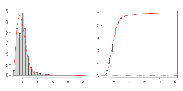
If is chosen to be the standard normal distribution, the corresponding polynomials are the (probabilists) Hermite polynomials. While the Hermite polynomials were used in Bladt et al. (2020) up to very high orders, their use in the following example fails already at low orders. This is likely caused by the tail of the normal distribution being too light. We propose a class of reference distributions based on a shifted beta distribution closely related to the Jacobi Polynomials as an alternative. This distribution will have finite support but a much heavier tail. Finite support is usually not a problem in a life insurance context.
Define a reference distribution with support on a finite interval by
Thus we need to find an orthonormal basis for . The starting point is the weight function
The space has an orthogonal basis of Jacobi polynomials given by
where denotes the Pochammer symbol.
By normalizing the weight function into a density on and then transforming it into a density on , we obtain an ONB for of polynomials given by
So for given , we need to compute
Here
where the inner expectation is computed as
Finally, the approximation is then given by
| (41) |
Concerning the corresponding distribution function, we integrate the above equation to obtain
Hence, these formulas can be used to approximate the density and distribution via these Jacobi types of polynomials.
6. Numerical Example
We now present a numerical example based on Example 5.1, where interest rates and biometric risk are assumed independent, where we carry over the estimation of interest transition rates from the calibrated bond prices of Section 3.
Consider the numerical example of Buchardt and Møller (2015) as the model for the biometric risk and corresponding life insurance contract. That is, the states of the insured are modelled as a time-inhomogeneous Markov jump process taking values , the three-state disability model depicted in Figure 7.
We consider a 40-year-old male today (at time ) with a retirement age of 65 and the following life insurance contract:
-
•
A disability annuity of rate while disabled until the retirement of age 65.
-
•
A life annuity of rate while alive until the retirement of age 65.
-
•
A constant premium rate paid while active until the retirement of age 65, priced under the equivalence principle at time .
The maximum contract time is , corresponding to a maximum age of 110 years. The transition rates are given by
The payment matrices for this product combination corresponds to having , and
For the stochastic interest rate model, we take the fitted bond prices from Example 4.1 with phases, so that the interest rates are given as , with
and where is a time-homogeneous Markov jump process taking values the finite state space with initial distribution and transition intensity matrix
We then determine the equivalence premium using the method outlined in Section 5.4. This is explicit on the form (40) due to being affine (for fixed ), and we get . This is almost three times lower than the premium rate obtained when pricing with a constant first-order interest rate of as in Buchardt and Møller (2015), which makes sense since the present interest rate model always gives interest rates above this level.
We then calculate moments of up to order 20 of the present value of future payments to approximate its density and distribution function via Gram-Charlier expansions based on the (shifted) Jacobi polynomials, as outlined in Section 5.5. The parameters used in the procedure are shown in Table 1, and the resulting density and distribution function are shown in Figure 8.
| Parameter | ||||
|---|---|---|---|---|
| Value | 1 | 0.05 | -3 | 70 |
From the fitted distribution function, one may compute different quantities of interest, e.g., quantiles of the present value. In Table 2, we show various quantiles based on the empirical (simulated) distribution function and the approximated distribution function based on 20 moments.
| Quantile | ||||
|---|---|---|---|---|
| Empirical | 3.51 | 5.51 | 9.51 | 12.01 |
| Moment-based | 3.13 | 5.54 | 8.89 | 12.63 |
Appendix A Modified EM algorithm for phase–type fitting with fixed exit rate vector
First, we consider the case we want to fit a phase–type distribution with parameters to data . Here the data are positive real numbers which are thought of as the time until absorption of the underlying Markov process with intensity matrix
We will assume throughout that , i.e. the Markov process is time–homogeneous. This presents no restriction as long as the interest rate process to be approximated is assumed to be stationary.
If, additionally to the absorption times, we could observe the full trajectories of the Markov process until absorption, then the estimation would be an easy task. In this case, for
| (42) |
whereas . Here denotes the number of processes starting in state , the number of transitions from to in all processes, the number of processes that exits to the absorbing state from state and the total time all processes spend in state .
In the case of incomplete data, where only absorption times are observed, the EM—algorithm can be employed. The idea is to replace the unobserved sufficient statistics , , and by the their conditional expectations given data, i.e. etc. The EM–algorithm then alternates between computing these conditional expected values (E–step) and plugging them into (42) as a substitute, thereby generating new parameters.
To perform maximization under the constraint , we see that this can be achieved simply by removing the update from the EM–algorithm, so that the –step amounts to
| (43) |
Fitting a PH distribution to a theoretical distribution is done by approximating the theoretical distribution into a histogram. Hence data will be the discretisation points, and the density values will be the corresponding weights. For further details on the EM–algorithm, we refer to Asmussen et al. (1996) or Albrecher et al. (2022).
Appendix B Proofs
Proof of Theorem 5.2.
First, we notice that, for ,
But on the event ,
Proof of Theorem 5.4.
Using that the product integral satisfies Kolmogorov’s forward and backward equations, we get that
from which Thiele’s differential equation can be pulled out from the upper right corner of each side of the equation. ∎
Proof of Theorem 5.6.
Write
| (44) | |||||
Now
and assume that is a point of increase for the counting process which trigger lump sum payments. Then in the computation of the above integral, there will be jump contributions at time , where any number of the variables may be equal to , say . We can pick out of the variables in ways. If variables coincide at the jump time , then a contribution of is added. Hence only looking at jump coincidences, i.e. , the contribution to the integral (44) is
Indeed, since there are precisely coincidences, the remaining integrals must start from ; otherwise, the integration intervals would contain as well. Changing the lower limits of the integrals appearing in the exponentials, we can further rewrite the expression as
| (45) |
Taking conditional expectation of (45), we get
| (46) | |||||
where and
Further conditioning on a lump sum triggering event at time , caused by and the probability of which is , and using that and are conditionally independent given , (46) reduces to
| (47) | |||||
Summing over and , and putting (47) on matrix form (in ) this amounts to
| (48) |
Now we consider the integral when there are no coincidences. To this end, we rewrite
References
- Albrecher et al. [2022] H. Albrecher, M. Bladt, and J. Yslas. Fitting inhomogeneous phase-type distributions to data: the univariate and the multivariate case. Scandinavian Journal of Statistics, 49(1):44–77, 2022.
- Asmussen and Steffensen [2020] S. Asmussen and M. Steffensen. Risk and Insurance. Series on Probability Theory and Stochastic Modelling. Springer, Cham, 2020.
- Asmussen et al. [1996] S. Asmussen, O. Nerman, and M. Olsson. Fitting phase-type distributions via the EM algorithm. Scandinavian Journal of Statistics, 23(4):419–441, 1996.
- Baños [2020] D.R. Baños. Life insurance policies with cash flows subject to random interest rate changes. arXiv:2012.15541, 2020.
- Bharucha-Reid [1960] A.T. Bharucha-Reid. Elements of the theory of Markov processes and their applications. McGraw-Hill series in probability and statistics. McGraw-Hill, New York, NY, 1960.
- Björk [2009] T. Björk. Arbitrage Theory in Continuous Time. Oxford Finance Series. Oxford University Press, third edition, 2009.
- Bladt and Nielsen [2017] M. Bladt and B.F. Nielsen. Matrix-Exponential Distributions in Applied Probability, volume 81 of Probability Theory and Stochastic Modelling. Springer, New York, NY, 2017.
- Bladt et al. [2020] M. Bladt, S. Asmussen, and M. Steffensen. Matrix representations of life insurance payments. European actuarial journal, 10(1):29–67, 2020.
- Brigo and Mercurio [2006] D. Brigo and F. Mercurio. Interest Rate Models: Theory and Practice ; With Smile, Inflation and Credit. Springer finance. Springer-Verlag, Berlin, Heidelberg, 2. aufl. edition, 2006.
- Buchardt [2014] K. Buchardt. Dependent interest and transition rates in life insurance. Insurance: Mathematics and Economics, 55:167–179, 2014.
- Buchardt and Møller [2015] K. Buchardt and T. Møller. Life Insurance Cash Flows with Policyholder Behavior. Risks, 3(3):290–317, 2015.
- Buchardt et al. [2020] K. Buchardt, C. Furrer, and T. Møller. Tax- and expense-modified risk-minimization for insurance payment processes. Scandinavian Actuarial Journal, 2020(10):934–961, 2020.
- Diez and Korn [2020] F. Diez and R. Korn. Yield curve shapes of vasicek interest rate models, measure transformations and an application for the simulation of pension products. European Actuarial Journal, 10(1):91–120, 2020.
- Elliott and Kopp [1999] R.J. Elliott and P.E. Kopp. Mathematics of financial markets. Springer finance. Springer, Berlin, 1999.
- Graham [1981] A. Graham. Kronecker products and matrix calculus : with applications. Ellis Horwood series in mathematics and its applications. Ellis Horwood, Chichester, NY, 1981.
- Hoem [1969] J.M. Hoem. Markov chain models in life insurance. Blätter der DGVFM, 9:91–107, 1969.
- Kalashnikov and Norberg [2003] V. Kalashnikov and R. Norberg. On the sensitivity of premiums and reserves to changes in valuation elements. Scandinavian Actuarial Journal, 2003(3):238–256, 2003.
- Koller [2012] M. Koller. Stochastic Models in Life Insurance. EAA series. Springer-Verlag, Berlin, Heidelberg, 2012.
- Kurtz [1970] T.G. Kurtz. Solutions of ordinary differential equations as limits of pure jump Markov processes. Journal of applied Probability, 7(1):49–58, 1970.
- Kurtz [1978] T.G. Kurtz. Strong approximation theorems for density dependent Markov chains. Stochastic Processes and their Applications, 6(3):223–240, 1978.
- Mijatović and Pistorius [2013] A. Mijatović and M. Pistorius. Continuously monitored barrier options under Markov processes. Mathematical Finance: An International Journal of Mathematics, Statistics and Financial Economics, 23(1):1–38, 2013.
- Møller and Steffensen [2007] T. Møller and M. Steffensen. Market-valuation methods in life and pension insurance. International Series on Actuarial Science. Cambridge University Press, Cambridge, 2007.
- Norberg [1991] R. Norberg. Reserves in Life and Pension Insurance. Scandinavian Actuarial Journal, 1991:3–24, 1991.
- Norberg [1995a] R. Norberg. Differential equations for moments of present values in life insurance. Insurance: Mathematics and Economics, 17(2):171–180, 1995a.
- Norberg [1995b] R. Norberg. A time-continuous Markov chain interest model with applications to insurance. Applied stochastic models and data analysis, 11(3):245–256, 1995b.
- Norberg [2003] R. Norberg. The Markov chain market. ASTIN Bulletin, 33(2):265–287, 2003.
- Norberg [2005] R Norberg. Anomalous PDEs in Markov chains: Domains of validity and numerical solutions. Finance and stochastics, 9(4):519–537, 2005.
- Norberg and Møller [1996] R. Norberg and C.M. Møller. Thiele’s differential equation with stochastic interest of diffusion type. Scandinavian Actuarial Journal, 1996(1):37–49, 1996.