Novel relaxation time approximation: a consistent calculation of transport coefficients with QCD-inspired relaxation times

Abstract

We use a novel formulation of the relaxation time approximation to consistently calculate the bulk and shear viscosity coefficients using QCD-inspired energy-dependent relaxation times and phenomenological thermal masses obtained from fits to lattice QCD thermodynamics. The matching conditions are conveniently chosen to simplify the computations.

1 Introduction

Nuclear matter in extreme conditions can be investigated through ultra-relativistic heavy-ion collisions. In particular, obtaining the transport coefficients of the quark-gluon plasma, throughout the QCD phase diagram, is a very challenging task that is currently beyond the reach of first-principles techniques [1]. In this contribution, we compute the transport coefficients of an effective kinetic model [2, 3] with a temperature-dependent mass whose equation of state mimics lattice QCD thermodynamics [4]. We use the new relaxation time approximation (RTA) of the relativistic Boltzmann equation proposed in [5] and impose alternative matching conditions such that the interaction energy [6] depends only on the temperature even out of equilibrium.

2 The quasi-particle model

The relativistic Boltzmann equation for quasi-particles with a temperature-dependent mass, $M(T)$, is given by [7],

$$p^{\mu}\partial_{\mu}f_{\bf p}+\frac{1}{2}\partial_{i}M^{2}(T)\partial^{i}_{(\bf p)}f_{\bf p}=C\left[f_{\bf p}\right],$$ (1)

where $f_{\bf p}=f(x,\bf{p})$ is the single particle distribution function. Above, $\partial^{i}_{(\bf p)}=\partial/\partial\mathbf{p}_{i}$, and $C\left[f_{\bf p}\right]$ is the collision integral.

In the limit of vanishing net-charge, the main dynamical equation is the continuity equation for the energy-momentum tensor, $T^{\mu\nu}$,

$$\partial_{\mu}T^{\mu\nu}=0.$$ (2)

In the presence of a thermal mass, $T^{\mu\nu}\equiv\langle p^{\mu}p^{\nu}\rangle+g^{\mu\nu}B$, where $B$ is the interaction energy [6], $g^{\mu\nu}$ denotes the metric, $\langle\cdots\rangle=\int dP\cdots f_{\bf p}$, $\int dP=g\int d^{3}\mathbf{p}/[(2\pi)^{3}E_{\bf p}]$, with $g$ being the degeneracy factor and $E_{\bf{p}}=\sqrt{\mathbf{p}^{2}+M^{2}}$. The interaction energy $B$ satisfies the following dynamical equation,

$$\partial_{\mu}B=-\frac{1}{2}\partial_{\mu}M^{2}\langle 1\rangle,$$ (3)

which is valid both in and out of equilibrium. We consider Maxwell-Boltzmann statistics so that in equilibrium $f_{\bf{p}}=\exp\left(-\beta u_{\mu}p^{\mu}\right)\equiv f_{0\bf{p}}$, with $\beta=1/T$ and $u_{\mu}$ being the fluid 4-velocity (which satisfies $u_{\mu}u^{\mu}=1$).

The temperature dependence of the mass is obtained such that the equation of state of the model describes lattice QCD results [4]. Plots for $B(T)$ and $M(T)$ can be seen in Refs. [2, 3]. Qualitatively, $M(T)/T$ is very large at low temperatures and saturates at $M(T)/T\approx 1.1$ at high temperatures.

3 Matching conditions and the collision term

The energy-momentum tensor can be decomposed in terms of the 4-velocity $u^{\mu}$ as follows

$$T^{\mu\nu} =\varepsilon u^{\mu}u^{\nu}-P\Delta^{\mu\nu}+h^{\mu}u^{\nu}+h^{\nu}u^{\mu}+\pi^{\mu\nu},$$ (4)

where $\varepsilon$ is the total energy density, $P$ is the total isotropic pressure, $h^{\mu}$ is the energy diffusion, $\pi^{\mu\nu}$ is the shear-stress tensor, and we defined the projection operator $\Delta^{\mu\nu}=g^{\mu\nu}-u^{\mu}u^{\nu}$. They are obtained from moments of $f_{\bf p}$ as explained in [7]. In general, $\varepsilon_{0}$ and $P_{0}$ may have non-equilibrium corrections, such that $\varepsilon=\varepsilon_{0}+\delta\varepsilon$, $P=P_{0}+\Pi$, respectively.

The meaning of $u^{\mu}$ and $\beta$ for non-equilibrium states is determined by matching conditions [7]. The most widely used prescription is the one introduced by Landau [8], where $\delta\varepsilon\equiv 0$ and $h^{\mu}\equiv 0$. In the present work, we choose a new prescription in order to simplify Eq. (3). Specifically, we impose

$$\left\langle 1\right\rangle\equiv\left\langle 1\right\rangle_{0},$$ (5)

where $\left\langle\cdots\right\rangle_{0}\equiv\int dP\cdots f_{0\mathbf{p}}$, which defines the temperature for non-equilibrium states. In this matching, $\delta\varepsilon\neq 0$. To define the 4-velocity, a further condition is needed. However, since we only consider a fluid at vanishing chemical potential, our results will not depend on this particular choice.

With prescription (5), the interaction energy can be determined solely as a function of $T$ and Eq. (3) can be solved as if the system were in equilibrium,

$$\frac{\partial B(T)}{\partial T}=-\frac{gTM^{2}}{2\pi^{2}}K_{1}\left(\frac{M(T)}{T}\right)\frac{\partial M(T)}{\partial T},$$ (6)

which can be readily integrated since $M(T)$ is known, and the boundary condition $B(0)=0$ is given. Above, $K_{1}$ is the first modified Bessel function of the second kind.

Novel relaxation time approximation

In contrast to the traditional RTA [9], in the new prescription proposed in Ref. [5] the conservation laws hold at the microscopic level even when considering momentum-dependent relaxation times and arbitrary matching conditions. In practice, we approximate the collision term as [3]

$$C[f_{\mathbf{p}}]\approx-\frac{E_{\mathbf{p}}}{\tau_{R}}f_{0\textbf{p}}\left[\phi_{\mathbf{p}}-\frac{\left\langle\phi_{\mathbf{p}}\frac{E_{\mathbf{p}}^{2}}{\tau_{R}}\right\rangle_{0}}{\left\langle\frac{E_{\mathbf{p}}^{3}}{\tau_{R}}\right\rangle_{0}}E_{\bf p}-\frac{\left\langle\phi_{\mathbf{p}}\frac{E_{\mathbf{p}}}{\tau_{R}}p^{\langle\mu\rangle}\right\rangle_{0}}{\frac{1}{3}\left\langle\Delta^{\alpha\beta}p_{\alpha}p_{\beta}\frac{E_{\mathbf{p}}}{\tau_{R}}\right\rangle_{0}}p_{\langle\mu\rangle}\right],$$ (7)

where $\phi_{\bf p}\equiv(f_{\bf p}-f_{0\bf p})/f_{0\bf p}$. We parametrize the energy dependence of the relaxation time as $\tau_{R}=t_{R}\left(E_{\mathbf{p}}/T\right)^{\gamma}$, where the parameter $\gamma$ encodes the information of the underlying microscopic interaction, and $t_{R}>0$. For instance, it has been argued that $\gamma=1/2$ in QCD effective theories [10]. Above, we defined the space-like projection $p^{\langle\mu\rangle}=\Delta^{\mu\nu}p_{\nu}$.

4 Transport coefficients

In first order theories, equation (2) is complemented by constitutive relations for the non-equilibrium currents ($\delta\varepsilon$, $\Pi$, $\pi^{\mu\nu}$). In kinetic theory, they can be calculated using the Chapman-Enskog expansion [7] which, when truncated at first order, leads to the following relativistic Navier-Stokes formulation of hydrodynamics,

$$\delta\varepsilon=\chi\theta,\quad\Pi=-\zeta\theta,\quad\pi^{\mu\nu}=2\eta\sigma^{\mu\nu}.$$ (8)

Using (7), the transport coefficients read [3]

$$\zeta=-\frac{1}{3}\left\langle\left(\Delta^{\mu\nu}p_{\mu}p_{\nu}\right)A_{\mathbf{p}}\frac{\tau_{R}}{E_{\mathbf{p}}}\right\rangle_{0}-\left\langle\frac{\tau_{R}}{E_{\mathbf{p}}}A_{\mathbf{p}}\right\rangle_{0}\frac{I_{3,1}}{I_{1,0}},$$ (9)

$$\chi=-\left\langle A_{\mathbf{p}}\tau_{R}E_{\mathbf{p}}\right\rangle_{0}+\left\langle\frac{\tau_{R}}{E_{\mathbf{p}}}A_{\mathbf{p}}\right\rangle_{0}\frac{I_{3,0}}{I_{1,0}},\quad\eta=\frac{\beta}{15}\left\langle\left(\Delta^{\mu\nu}p_{\mu}p_{\nu}\right)^{2}\frac{\tau_{R}}{E_{\mathbf{p}}}\right\rangle_{0},$$

where $A_{\mathbf{p}}=-\beta c_{s}^{2}E_{\bf p}^{2}-\frac{\beta}{3}\Delta^{\lambda\sigma}p_{\lambda}p_{\sigma}-\beta^{2}M\frac{\partial M}{\partial\beta}c_{s}^{2}$, and $c_{s}^{2}\equiv\left(\partial P_{0}/\partial\varepsilon_{0}\right)=\\ (1/\beta)(I_{10}+I_{21})/[I_{30}+\frac{1}{2}I_{10}(\partial M^{2}/\partial\beta)\beta]$ is the speed of sound squared, which is expressed in terms of $I_{nq}=1/[(2q+1)!!]\left\langle\left(-\Delta^{\lambda\sigma}p_{\lambda}p_{\sigma}\right)^{q}E_{\mathbf{p}}^{n-2q}\right\rangle_{0}$.

In Fig. 1 we plot the coefficients as functions of temperature for different values of the parameter $\gamma$, as well as the temperature dependence of the mass. For all values of $\gamma$ investigated, $\zeta\geq 0$ and $\chi\leq 0$. In both figures, it is seen that the absolute values of the coefficients grow with $\gamma$. At low temperatures, where the effective mass is large, $M/T\rightarrow\infty$, all three normalized coefficients behave as $(M/T)^{\gamma-1}$. For $\gamma=1$, $\eta=t_{R}(\varepsilon_{0}+P_{0})$ at all temperatures. In the opposite limit, $M/T\rightarrow 0$, $\zeta=-(1/3)\chi\propto M(T)(d/dT)\left(M(T)/T\right)$ and $\eta\sim\Gamma(\gamma+5)/120$ .

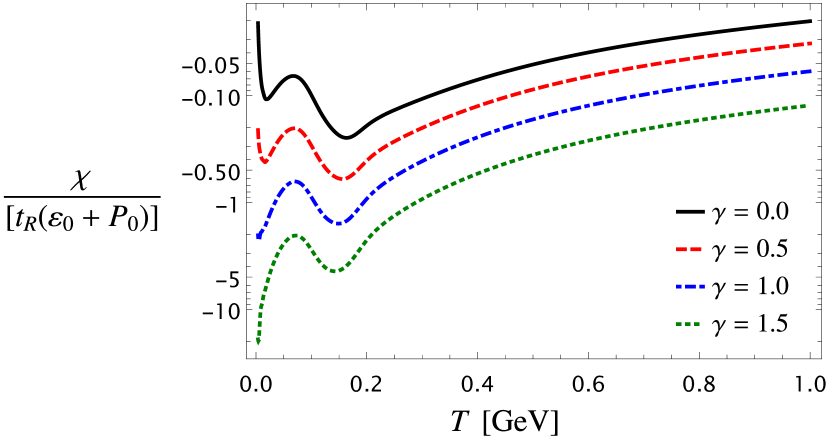
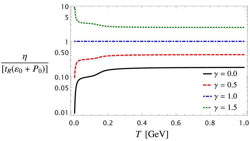
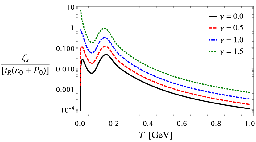
Figure 1: (Top left) Normalized bulk viscosity, (Top right) energy correction coefficient, (Bottom left) shear viscosity, and (Bottom right) matching-invariant bulk viscosity coefficients as functions of temperature. Each transport coefficient is shown for various values of the parameter $\gamma$.

Entropy production

The entropy current for classical quasiparticles is $S^{\mu}=\int dPp^{\mu}f_{\bf p}(1-\ln f_{\bf p})$. We note that the entropy production does not depend on the choice of matching conditions [3]. To first order in the Chapman-Enskog expansion, one finds

$$\partial_{\mu}S^{\mu}\simeq\zeta_{s}\theta^{2}+2\eta\sigma^{\mu\nu}\sigma_{\mu\nu},\quad\zeta_{s}=\left\langle\frac{\tau_{R}}{E_{\bf p}}[A_{\bf p}]^{2}\right\rangle_{0}=\zeta+c_{s}^{2}\chi.$$ (10)

Since both $\zeta_{s}$ and $\eta$ are non-negative, so is the entropy production. The coefficient $\zeta_{s}$ can be used to provide a matching-invariant interpretation of bulk viscosity and, indeed, for Landau matching conditions $\zeta_{s}=\zeta$. This coefficient behaves similarly to $\zeta$ as a function of temperature, with the difference that, as $M/T\rightarrow 0$, $\zeta_{s}\propto[M(T)(d/dT)\left(M(T)/T\right)]^{2}$, thus displaying a steeper descent at high temperatures in Fig. 1.

5 Conclusion

In this work we have computed the first-order transport coefficients of an effective kinetic model with temperature-dependent mass, using the new relaxation time approximation proposed in Ref. [5]. We have used an alternative matching condition [Eq. (5)] to simplify the computations, which in turn imply that there are nonzero out-of-equilibrium corrections to the energy density. We find that all transport coefficients are significantly affected by the choice of the parameter $\gamma$, which defines how the relaxation time depends on energy. Consistency with the second law of thermodynamics is demonstrated and used to derive a matching-invariant bulk viscosity coefficient. In future work, we intend to compute the transport coefficients that appear in other theories of hydrodynamics [11, 12] using the present model.

References

- [1] H. B. Meyer, “Transport Properties of the Quark-Gluon Plasma: A Lattice QCD Perspective,” Eur. Phys. J. A, vol. 47, p. 86, 2011.
- [2] M. Alqahtani, M. Nopoush, and M. Strickland, “Quasiparticle equation of state for anisotropic hydrodynamics,” Phys. Rev. C, vol. 92, no. 5, p. 054910, 2015.
- [3] G. S. Rocha, M. N. Ferreira, G. S. Denicol, and J. Noronha, “Determining the transport coefficients of the quark-gluon plasma using a new relaxation time approximation of the Boltzmann equation,” arXiv:2203.15571 2022.
- [4] S. Borsanyi, G. Endrodi, Z. Fodor, A. Jakovac, S. D. Katz, S. Krieg, C. Ratti, and K. K. Szabo, “The QCD equation of state with dynamical quarks,” JHEP, vol. 11, p. 077, 2010.
- [5] G. S. Rocha, G. S. Denicol, and J. Noronha, “Novel Relaxation Time Approximation to the Relativistic Boltzmann Equation,” Phys. Rev. Lett., vol. 127, no. 4, p. 042301, 2021.
- [6] S. Jeon and L. G. Yaffe, “From quantum field theory to hydrodynamics: Transport coefficients and effective kinetic theory,” Phys. Rev. D, vol. 53, pp. 5799–5809, 1996.
- [7] G. Denicol and D. H. Rischke, Microscopic Foundations of Relativistic Fluid Dynamics. Springer, 2021.
- [8] L. Landau and E. Lifshitz, “Fluid Mechanics,” Course of Theoretical Physics, Pergamon Press, London, vol. 6, 1959.
- [9] J. L. Anderson and H. Witting, “A relativistic relaxation-time model for the Boltzmann equation,” Physica, vol. 74, no. 3, pp. 466–488, 1974.
- [10] K. Dusling, G. D. Moore, and D. Teaney, “Radiative energy loss and v 2 spectra for viscous hydrodynamics,” Physical Review C, vol. 81, no. 3, p. 034907, 2010.
- [11] G. S. Denicol, H. Niemi, E. Molnar, and D. H. Rischke, “Derivation of transient relativistic fluid dynamics from the Boltzmann equation,” Phys. Rev. D, vol. 85, p. 114047, 2012, [Erratum: Phys.Rev.D 91, 039902 (2015)].
- [12] F. S. Bemfica, M. M. Disconzi, and J. Noronha, “Causality and existence of solutions of relativistic viscous fluid dynamics with gravity,” Phys. Rev. D, vol. 98, no. 10, p. 104064, 2018.