NLO QCD and EW corrections to off-shell tZj production at the LHC

Abstract

The production of a single top quark in association with a Z boson (tZj production) at the LHC is a relevant probe of the electroweak sector of the Standard Model as well as a window to possible new-physics effects. The growing experimental interest in performing differential measurements for this process demands an improved theoretical modelling in realistic fiducial regions. In this article we present an NLO-accurate tZj calculation that includes complete off-shell effects and spin correlations, combining QCD and electroweak radiative corrections to the LO signal. Integrated and differential cross sections are shown for a fiducial setup characterised by three charged leptons, two jets, and missing energy.

1 Introduction

The production of a single top quark in association with a Z boson is well suited to directly study the electroweak (EW) interactions between two of the heaviest particles in the Standard Model (SM).

Differently from processes involving top–anti-top-quark pairs, which are typically dominated by QCD production mechanisms, single-top processes are mediated by the EW interaction. Therefore they have smaller cross sections, but also smaller theoretical uncertainties. The standard signature for single-top processes is characterised by a top quark (followed by its leptonic or hadronic decay) and an additional jet (often labelled as spectator jet), produced in association with zero, one, or more EW bosons ($\text{W},\,\text{Z},\,\text{H}$).

The tZj process is among the very few ones that give direct access to the top-quark coupling to Z bosons. This interaction is poorly known, and a lot of effort is being put into its investigation both from the experimental and from the theoretical side. Despite having a similar total cross section as $\text{t}\bar{\text{t}}\text{Z}$ production, tZj production is more suitable to study the $\text{t}\bar{}\text{t}\text{Z}$ coupling as tZj is an EW process, while $\text{t}\bar{\text{t}}\text{Z}$ production is QCD dominated. Moreover, tZj production gives access to the triple-gauge (WWZ) coupling and via the decay of the top quark to the tWb coupling. Owing to the EW-mediated production, the top quark in tZj production is typically polarised, and therefore the measurements of polarisation-sensitive observables and the extraction of helicity fractions provide additional probes of the SM and possible deviations from it Mahlon:1999gz .

The importance of tZj as a signal process is shown by several dedicated LHC measurements performed by CMS and ATLAS with the 13 TeV dataset CMS:2017wrv ; ATLAS:2017dsm ; CMS:2018sgc ; ATLAS:2020bhu ; CMS:2021ugv . The measurement of the total tZj cross section CMS:2018sgc ; ATLAS:2020bhu ; CMS:2021ugv , found to be in good agreement with the SM prediction, represents an important stress-test of the SM, but performing differential measurements is expected to give an enhanced sensitivity to possible deviations of top-quark couplings from their SM values Degrande:2018fog . Therefore it is essential that the theoretical predictions account for the modelling of the decays of the involved resonances.

From the theory side, SM predictions are currently limited to on-shell approximations for the top-quark description. The next-to-leading-order (NLO) QCD corrections in the SM are known for many years in the approximation where the production and decay are factorised Campbell:2013yla . Combined NLO EW+QCD corrections in the SM have been computed for an on-shell top quark and off-shell Z boson, including also parton-shower effects Pagani:2020mov . As other single-top processes, tZj production is suited to compare the five-flavour and four-flavour schemes Pagani:2020mov and therefore to study the b-quark contribution to the proton structure Campbell:2021qgd . Phenomenological investigations of the tZj process have been performed in the presence of new-physics effects, with a focus on vector-like top partners Reuter:2014iya and anomalous $\text{t}\text{Z}q$ couplings Li:2011ek ; Kidonakis:2017mfy ; Liu:2020bem . A detailed analysis in the SM effective field theory has been carried out in Refs. Degrande:2018fog ; Barman:2022vjd , where the combination of tZj and tHj processes has been shown to enhance the sensitivity to anomalous values of several SM couplings.

The presented calculation provides the first complete off-shell SM prediction at NLO QCD+EW accuracy in the five-flavour scheme. The modelling of the top-quark and Z-boson decays accounts for all resonant and non-resonant contributions and includes complete spin correlations, both at LO and at NLO. An interesting feature of the off-shell calculation is that, although at LO the final-state signature selects the decay products of a (leptonically-decaying) top quark, the real corrections at NLO (both QCD and EW) inevitably include partonic processes featuring a (hadronically-decaying) anti-top quark. These contributions, which are absent in on-shell-approximated calculations, turn out to be quantitatively important.

The paper is organised as follows. In Sect. 2 we describe the details of our perturbative calculation, the input SM parameters and the employed fiducial selection cuts, as well as the reconstruction techniques adopted for the jet and neutrino kinematics. The integrated cross sections and a number of differential distributions are discussed in Sect. 3. In Sect. 4 we draw the conclusions.

2 Details of the calculation

2.1 Description of the process

Following the signal definition of recent LHC analyses ATLAS:2020bhu ; CMS:2021ugv , we consider the processes

$$\text{p}\text{p}\rightarrow\text{e}^{+}\text{e}^{-}\mu^{+}\nu_{\mu}{\rm J}\,{\rm j_{\text{b}}}\,+X\,,$$ (1)

at NLO EW and QCD accuracy, where ${\rm j_{\text{b}}}$ stands for a b jet, and ${\rm J}$ could be either a light jet or another b jet ($\rm J=j_{b},j$). In the five-flavour scheme, the LO process receives contributions from partonic channels that only involve quarks as external coloured particles:

$$\bar{q}_{\text{d}}\,q_{\text{u}}\rightarrow\bar{\text{b}}\,\text{b}\ \text{e}^{+}\text{e}^{-}\mu^{+}\nu_{\mu}\,,\qquad q_{\text{u}}\overset{\scriptscriptstyle(-)}{\text{b}}\rightarrow{q}_{\text{d}}\overset{\scriptscriptstyle(-)}{\text{b}}\ \text{e}^{+}\text{e}^{-}\mu^{+}\nu_{\mu}\,,\qquad\bar{q}_{\text{d}}\overset{\scriptscriptstyle(-)}{\text{b}}\rightarrow\bar{q}_{\text{u}}\overset{\scriptscriptstyle(-)}{\text{b}}\ \text{e}^{+}\text{e}^{-}\mu^{+}\nu_{\mu}\,.$$

At cross-section level, three tree-level perturbative orders are present, namely $\mathcal{O}(\alpha^{6})$, $\mathcal{O}(\alpha_{\text{s}}^{2}\alpha^{4})$, and the interference $\mathcal{O}(\alpha_{\text{s}}\alpha^{5})$. However, the EW production of a top quark and a Z boson can only take place at $\mathcal{O}(\alpha^{6})$, which is in fact regarded as the LO signal. The interference, of $\mathcal{O}(\alpha_{\text{s}}\alpha^{5})$, vanishes due to colour algebra, since the mixing of the bottom quark with the light quarks is neglected (a unit CKM matrix is assumed). The $\mathcal{O}(\alpha_{\text{s}}^{2}\alpha^{4})$ contributions and NLO corrections on top of them are not considered in this paper.

With the signal definition of Eq. (1), it is easy to see that the production of an (off-shell) top quark can take place both in $s$ channel ($\bar{q}_{\text{d}}\,q_{\text{u}}$ initial state) and in $t$ channel ($q_{\text{u}}\overset{\scriptscriptstyle(-)}{\text{b}},\,\bar{q}_{\text{d}}\overset{\scriptscriptstyle(-)}{\text{b}}$ initial states). Sample diagrams are shown in Fig. 1.

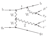
(a) $t$ channel

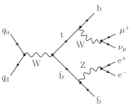
(b) $s$ channel

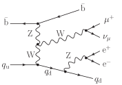
(c) Non resonant

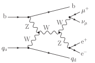
(d) Vector-boson scattering

Figure 1: Sample tree-level diagrams contributing at $\mathcal{O}(\alpha^{6})$ to off-shell tZj production at the LHC.

It is essential to recall that at LO a clear distinction between $s$- and $t$-channel contributions is possible, owing to a different number of b quarks in the final state [see Figs. 1(a)–1(b)]. However, starting from NLO corrections (both QCD and EW), such a separation between the two top-quark production mechanisms is ill defined, i.e. the different contributions are not separately gauge invariant owing to partonic channels that embed both $s$- and $t$-channel contributions, as in off-shell single-top production Falgari:2011qa ; Frederix:2019ubd . All resonant and non-resonant [Fig. 1(c)] contributions are included for all partonic channels. Contributions without a top-quark resonance as those embedding the vector-boson scattering subprocess [Fig. 1(d)] are expected to be sub-dominant w.r.t. the top-quark-resonant ones.

At NLO there are four different perturbative orders, but in this paper we only consider corrections of $\mathcal{O}(\alpha^{7})$ and $\mathcal{O}(\alpha_{\text{s}}\alpha^{6})$. The former are genuine EW corrections to the leading EW order. The latter naively include two kinds of corrections: the QCD corrections to the leading EW order and the EW ones to the LO interference. However, since virtual or real EW corrections do not change the vanishing colour structure of the LO interference, the $\mathcal{O}(\alpha_{\text{s}}\alpha^{6})$ is only made of pure QCD corrections to the LO EW contribution.

The following real partonic processes contribute at $\mathcal{O}(\alpha_{\text{s}}\alpha^{6})$:

$$\bar{q}_{\text{d}}\,q_{\text{u}} \rightarrow\bar{\text{b}}\,\text{b}\ \text{g}\ \text{e}^{+}\text{e}^{-}\mu^{+}\nu_{\mu}\,,\quad q_{\text{u}}\overset{\scriptscriptstyle(-)}{\text{b}}\rightarrow{q}_{\text{d}}\overset{\scriptscriptstyle(-)}{\text{b}}\ \text{g}\ \text{e}^{+}\text{e}^{-}\mu^{+}\nu_{\mu}\,,\quad\bar{q}_{\text{d}}\overset{\scriptscriptstyle(-)}{\text{b}}\rightarrow\bar{q}_{\text{u}}\overset{\scriptscriptstyle(-)}{\text{b}}\ \text{g}\ \text{e}^{+}\text{e}^{-}\mu^{+}\nu_{\mu}\,,$$

$$\text{g}\,q_{\text{u}} \rightarrow\bar{\text{b}}\,\text{b}\ {q}_{\text{d}}\ \text{e}^{+}\text{e}^{-}\mu^{+}\nu_{\mu}\,,\quad\bar{q}_{\text{d}}\,\text{g}\rightarrow\bar{\text{b}}\,\text{b}\ \bar{q}_{\text{u}}\ \text{e}^{+}\text{e}^{-}\mu^{+}\nu_{\mu}\,,\quad\,\,\text{g}\ \overset{\scriptscriptstyle(-)}{\text{b}}\rightarrow\bar{q}_{\text{u}}\,{q}_{\text{d}}\,\overset{\scriptscriptstyle(-)}{\text{b}}\ \text{e}^{+}\text{e}^{-}\mu^{+}\nu_{\mu}\,.$$

The same processes contribute at $\mathcal{O}(\alpha^{7})$, upon replacing external gluons with photons. The gluon-induced channels that open up at NLO QCD give a sizeable contribution owing to the enhancement from the large gluon luminosity in the proton. In contrast, the photon-induced real corrections are suppressed by coupling power counting $[\mathcal{O}(\alpha/\alpha_{\text{s}})]$ and by the small photon luminosity in the proton.

The new partonic channels that contribute at NLO can also enhance the cross section due to different underlying resonance structures with respect to those present at LO. In particular, the processes

$$\bar{\text{b}}\,\text{g},\,\bar{\text{b}}\,\gamma\rightarrow\bar{q}_{\text{u}}\,{q}_{\text{d}}\,\bar{\text{b}}\ \text{e}^{+}\text{e}^{-}\mu^{+}\nu_{\mu}$$ (2)

allow for the production of a resonant anti-top quark followed by its hadronic decay ($\bar{\text{t}}\rightarrow\bar{q}_{\text{u}}\,{q}_{\text{d}}\,\bar{\text{b}}$), as shown in the sample diagram in Fig. 2.

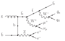
Figure 2: Sample diagram for anti-top-quark production in the $\text{g}\bar{\text{b}}$ channel at $\mathcal{O}(\alpha_{\text{s}}\alpha^{6})$.

Such a contribution, which is absent in on-shell-approximated calculations Campbell:2013yla ; Pagani:2020mov , is non-negligible and could be suppressed using a jet veto requiring at most one light jet. Since the same considerations hold for the charge-conjugated process of Eq. (1), if both tZj and $\bar{\text{t}}\text{Z}\text{j}$ production were included in the signature as in experimental analyses CMS:2017wrv ; ATLAS:2017dsm ; CMS:2018sgc ; ATLAS:2020bhu ; CMS:2021ugv ,

$$\text{p}\text{p}\rightarrow\text{e}^{+}\text{e}^{-}\mu^{\pm}\overset{\scriptscriptstyle(-)}{\nu}_{\!\!\mu\,}{\rm J}\,{\rm j_{\text{b}}}\,+X\,,$$ (3)

the contributions from $\bar{\text{t}}\text{W}^{+}\text{Z}$ and ${\text{t}}\text{W}^{-}\text{Z}$ intermediate states would both give a similar relative correction to the respective cross section.

The analysis of the initial-state singularities in gluon-induced channels also shows that a distinction between $s$- and $t$-channel contributions is not well defined at NLO. In Fig. 3 we highlight the underlying Born-level processes that are embedded in the real-radiation channel $\text{g}q_{\text{u}}$.

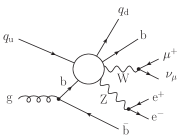
(a) $\text{g}\rightarrow\text{b}\bar{\text{b}}$

(b) $\text{g}\rightarrow\bar{\text{b}}\text{b}$

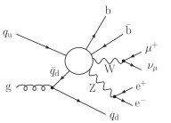
(c) $\text{g}\rightarrow\bar{q}_{\text{d}}q_{\text{d}}$

Figure 3: Real-radiation topologies embedding different initial-state collinear splittings in the $\text{g}q_{\text{u}}$ channel at $\mathcal{O}(\alpha_{\text{s}}\alpha^{6})$.

Comparing the three topologies it is clear that the same real partonic process may include both $s$- and $t$-channel single-top diagrams, which are not separately gauge-invariant.

A large number of soft- and collinear-singular configurations need to be subtracted in order to render the calculation infrared safe, both at NLO QCD and at NLO EW. The number of subtraction terms is especially large in the $\mathcal{O}(\alpha^{7})$ corrections due to the presence of seven external charged particles at LO, while the number of subtraction terms needed at $\mathcal{O}(\alpha_{\text{s}}\alpha^{6})$ is smaller owing to only four coloured external particles at Born level. It is worth noticing that, thanks to the requirement of at least one b jet in the final state, it is not necessary to include subtraction terms for a $\gamma\rightarrow\bar{}\text{b}\text{b}$ splitting in the final state, which appears in gluon-induced real contributions. The collinear singularity associated with this splitting is in fact cut out thanks to a $\bar{\text{b}}{\text{b}}\rightarrow{\rm j}$ recombination condition that we apply to make the jet algorithm infrared safe also in the presence of flavoured jets Banfi:2006hf . The same argument holds at $\mathcal{O}(\alpha^{7})$ for photon–quark-induced partonic channels. See Sect. 2.3, in particular Eq. (13), for a more detailed discussion of the recombination algorithm.

The one-loop amplitudes that enter the virtual corrections both at NLO EW and at NLO QCD involve up to 8-point functions. However, in spite of the presence of several mass scales making the loop-integral evaluation more involved, the virtual corrections ($2\rightarrow 6$ process) are computationally less expensive than the real corrections ($2\rightarrow 7$ process).

The calculation is performed within the MoCaNLO Monte Carlo framework. MoCaNLO has already been used to compute full NLO corrections to LHC processes with a high number of particles in the final state, including underlying resonance structures with top quarks Denner:2015yca ; Denner:2016jyo ; Denner:2016wet ; Denner:2017kzu ; Denner:2020hgg ; Denner:2021hqi . MoCaNLO relies on tree-level and one-loop SM amplitudes provided by Recola Actis:2012qn ; Actis:2016mpe and computed with the help of the Collier library Denner:2016kdg for tensor-integral reduction Denner:2002ii ; Denner:2005nn and loop-integral evaluation Denner:2010tr . The dipole formalism Catani:1996vz ; Dittmaier:1999mb ; Catani:2002hc ; Dittmaier:2008md is employed to take care of the cancellation of soft and collinear singularities of QCD and QED origin. The $\overline{{\text{MS}}}$ factorisation scheme is used for the treatment of initial-state collinear singularities.

The presented calculation of the NLO QCD + EW corrections to tZj production can be viewed as complementary to the one of WZ scattering Denner:2019tmn , which has also been carried out in the MoCaNLO framework. The two calculations basically share the same final state [see Fig. 1(d)], the only difference being the minimum number of required b-tagged jets. However, the dominant resonance structure is different in the two processes, which motivates rather different kinematic selections and well-distinguished signal definitions in LHC analyses.

In this context we only focus on the perturbative orders that enable the presence of a top quark as underlying resonance, i.e. the EW signal, while we ignore the QCD background and NLO corrections to it. In spite of the absence of a resonant top quark, the QCD background ($\text{W}\text{Z}+$jets) is expected to be sizeable and thus deserves a tailored phenomenological study.

As a last comment of this section, we stress that all results presented in this paper are within the five-flavour scheme. This scheme has the advantage of resumming effectively the logarithms of the type $\alpha_{\text{s}}^{n}\log^{m}({\mu^{2}/m_{\text{b}}^{2}})$ for $m\leq n$, but the disadvantage of having at NLO QCD a leading-order-like renormalisation-scale dependence. Since the typical hard scale $\mu$ of the process is much larger than the b-quark mass, the power corrections of type $(m_{\text{b}}/\mu)^{n}$ can be safely neglected. A four-flavour calculation would include the complete $m_{\text{b}}$ dependence and provide an actual NLO scale dependence on the renormalisation scale when including QCD corrections Pagani:2020mov . In the four-flavour scheme gluon-initiated processes contribute already at LO, resulting in sizeable $\text{t}\bar{\text{t}}\text{Z}$ and tWZ contamination, which needs to be taken care by specific cuts and vetoes. Although a comparison between the two schemes including off-shell effects (see Ref. Pagani:2020mov for on-shell top quarks) is desirable, this is beyond the scope of this work.

2.2 Input parameters

We compute LO and NLO cross sections in the SM for the process defined in Eq. (1). All leptons are considered massless. The five-flavour scheme ($N_{\text{f}}=5$) is employed, and we therefore include contributions with initial-state b quarks, which are assumed to be massless as the other light quarks. A unit CKM matrix is used, leading to no mixing between different quark families. The values for the on-shell masses and widths of EW bosons are ParticleDataGroup:2020ssz ,

$$M_{\text{W}}^{\text{OS}} =80.379\,\text{GeV},\qquad \Gamma_{\text{W}}^{\text{OS}} =2.085\,\text{GeV},$$ (4)

$$M_{\text{Z}}^{\text{OS}} =91.1876\,\text{GeV},\qquad \Gamma_{\text{Z}}^{\text{OS}} =2.4952\,\text{GeV}.$$

The on-shell values are converted into the corresponding pole values according to the relations Bardin:1988xt

$$M_{V}=\frac{M_{V}^{\rm OS}}{\sqrt{1+\left(\Gamma_{V}^{\rm OS}/M_{V}^{\rm OS}\right)^{2}}}\,,\qquad\Gamma_{V}=\frac{\Gamma_{V}^{\rm OS}}{\sqrt{1+\left(\Gamma_{V}^{\rm OS}/M_{V}^{\rm OS}\right)^{2}}}\,.$$ (5)

The mass and width of the Higgs boson are set to the following values ParticleDataGroup:2020ssz ,

$$M_{\text{H}}={} 125\,\text{GeV},\qquad\Gamma_{\text{H}}=4.07\,\,\text{MeV}.$$ (6)

The NLO width of the top quark is used in all contributions to the cross section. We apply relative NLO EW and QCD corrections from Ref. Basso:2015gca to the LO top-quark width computed following Ref. Jezabek:1988iv . The numerical values read

$$m_{\text{t}}=173\,\text{GeV},\qquad\Gamma_{\text{t}}=1.3636\,\text{GeV}.$$ (7)

The EW coupling is defined in the $G_{\mu}$ scheme Denner:2000bj , with the Fermi constant set to

$$G_{\mu}=1.16638\cdot 10^{-5}\,\text{GeV}^{-2}.$$ (8)

EW-boson and top-quark masses, as well as of the EW mixing angle, are treated within the complex-mass scheme Denner:1999gp ; Denner:2000bj ; Denner:2005fg ; Denner:2006ic ; Denner:2019vbn .

The evaluation of parton-distribution functions (PDFs) and the running of $\alpha_{\text{s}}$ are performed with the LHAPDF6 interface Buckley:2014ana . We use the NNPDF31_nnlo_as_0118_luxqed PDF set Bertone:2017bme throughout the calculation.

The renormalisation and factorisation scales are simultaneously set to the following dynamical value,

$$\mu_{\rm R}^{0}=\mu_{\rm F}^{0}=\frac{M_{{\mathrm{T}},\text{t}}+M_{{\mathrm{T}},\text{Z}}}{6}\,,$$ (9)

adapting the choice of Ref. Pagani:2020mov to the inclusion of decay products of the top quark. In particular, we define the transverse mass of the Z boson as

$$M_{{\mathrm{T}},\text{Z}}=\sqrt{M_{\text{Z}}^{2}+\left(\vec{p}_{\rm T,e^{+}}+\vec{p}_{\rm T,e^{-}}\right)^{2}}\,.$$ (10)

If both tagged jets are b jets, the top-quark momentum is reconstructed with the b jet ($\rm j_{b}^{\rm best}$) that gives an invariant mass of the $\mu^{+}\nu_{\mu}\rm j_{b}$ system closest to the top-quark pole mass. If only one tagged b jet is present, it is automatically associated to the top quark, in a formula,

$$M_{{\mathrm{T}},\text{t}}=\sqrt{m_{\text{t}}^{2}+\left(\vec{p}_{\rm T,\mu^{+}}+\vec{p}_{\rm T,\nu_{\mu}}+\vec{p}_{\rm T,j_{b}^{\rm best}}\right)^{2}}\,.$$ (11)

When performing scale variations we vary $\mu_{\mathrm{R}}=\xi_{\mathrm{R}}\mu_{\mathrm{R}}^{0}$ and $\mu_{\mathrm{F}}=\xi_{\mathrm{F}}\mu_{\mathrm{F}}^{0}$ around the central choice $\mu_{\mathrm{R}}^{0}$ and $\mu_{\mathrm{F}}^{0}$ by the following factors $(\xi_{\mathrm{R}},\xi_{\mathrm{F}})$:

$$\bigl{(}1/2,1/2\bigr{)}\text{,}\quad\bigl{(}1,1\bigr{)}\text{,}\quad\bigl{(}2,2\bigr{)}\text{,}\quad\bigl{(}1,1/2\bigr{)}\text{,}\quad\bigl{(}1/2,1\bigr{)}\text{,}\quad\bigl{(}1,2\bigr{)}\text{,}\quad\bigl{(}2,1\bigr{)}\text{,}$$ (12)

and take the envelope (minimum and maximum value of the varied cross sections) to estimate the QCD uncertainty.

2.3 Selection cuts

Only particles (charged under QED or QCD) with $|y|<5$ undergo jet clustering, which is achieved using the $k_{{\mathrm{T}}}$ jet algorithm Catani:1991hj ; Catani:1993hr ; Ellis:1993tq with resolution radius $R=0.4$ and $R=0.1$, respectively, for jets (both at NLO QCD and NLO EW) and dressed leptons (at NLO EW). The $k_{{\mathrm{T}}}$ jet algorithm is chosen over the corresponding anti-$k_{{\mathrm{T}}}$ algorithm since the former is known to have an infrared-safe definition Banfi:2006hf at all orders in the presence of flavoured jets. Thus, we label jets as either light jets (j), or b jets ($\mathrm{j}_{\text{b}}$) using the following recombination rules:

$$\overset{\scriptscriptstyle(-)}{\text{b}}\text{g}\rightarrow{\text{j}}_{\text{b}}\text{,}\quad\overset{\scriptscriptstyle(-)}{\text{b}}\gamma\rightarrow{\text{j}}_{\text{b}}\text{,}\quad\bar{}\text{b}\,\text{b}\rightarrow{\text{j}}\text{,}\quad\text{g}\,\text{g}\rightarrow{\text{j}}\text{,}\quad\overset{\scriptscriptstyle(-)}{q}\text{g}\rightarrow{\text{j}}\text{,}\quad\overset{\scriptscriptstyle(-)}{q}\gamma\rightarrow{\text{j}}\text{,}\quad\ell^{\pm}\gamma\rightarrow{\ell^{\pm}}\text{.}$$ (13)

As introduced in Sect. 2.1 we follow the setup of the recent ATLAS analysis ATLAS:2020bhu . We ask for events with

$$N_{\rm J}=N_{\rm j}+N_{\rm j_{\text{b}}}\geq 2\,,\qquad N_{\rm j_{\text{b}}}\geq 1\,,$$ (14)

and assume 100% b-tagging efficiency. Jets are required to satisfy

$$p_{{\mathrm{T}},{\rm j}}>35\,\text{GeV},\qquad p_{{\mathrm{T}},{\rm j_{b}}}>35\,\text{GeV},\qquad|y_{\rm j}|<4.5\,,\qquad|y_{\rm j_{\text{b}}}|<2.5\,.$$ (15)

Furthermore, we ask for exactly three charged leptons ($\text{e}^{+}\text{e}^{-}\mu^{+}$) with

$$|y_{\ell^{\pm}}|<2.5\,,\qquad p_{{\mathrm{T}},{\ell_{1}}}>28\,\text{GeV},\qquad p_{{\mathrm{T}},{\ell_{2}}},\,p_{{\mathrm{T}},{\ell_{3}}}>20\,\text{GeV},$$ (16)

where the charged leptons are sorted according to their transverse momentum, $\ell_{1}$ being the leading one. The invariant mass of the opposite-sign, same-flavour lepton pair ($\text{e}^{+}\text{e}^{-}$ in our case) is constrained by setting

$$M_{\text{e}^{+}\text{e}^{-}}>30\,\text{GeV}.$$ (17)

A minimum distance is required between jets and charged leptons,

$$\Delta R_{\rm j,\ell}>0.4\,,\qquad\Delta R_{\rm j_{\text{b}},\ell}>0.4\,.$$ (18)

Besides the default setup just described, we consider a setup with an additional cut on the invariant mass of the $\text{e}^{+}\text{e}^{-}$ pair

$$$81\text{\,}\mathrm{GeV}$<M_{\mathrm{e}^{+}\mathrm{e}^{-}}<$101\text{\,}\mathrm{GeV}$\text{.}$$ (19)

This cut selects events close to the Z-boson resonance and is therefore called Z-peak setup.

2.4 Event topologies and kinematic reconstruction

Since we consider final states with more than one b-flavoured jet, the identification of the b jet from the top-quark decay is ambiguous. To properly define physical observables, we need to solve this ambiguity by means of some discrimination criterion.

In the considered setups, at least two jets are required to fulfil the selections described in Eqs. (15) and (18). At LO only two-jet events are present. At NLO, the additional QCD or photon radiation may be clustered with other partons (giving a two-jet event) or result in a third jet. If also the third jet fulfils the requirements of Eqs. (15) and (18), we have a three-jet event, otherwise we have a two-jet event.

The definitions we use for the top-decay jet (${\rm j}_{\rm t}$) and for the spectator jet (${\rm j}_{\rm s}$) are inspired by single-top NLO studies Cao:2005pq ; Schwienhorst:2010je and mimic those used in the most recent CMS analysis CMS:2021ugv .

In the case of a two-jet event with one b jet and one light jet, there is no ambiguity, therefore the b jet is labelled as the top-decay jet, while the light jet is labelled as the spectator jet. If both jets are b jets, the top-decay jet is the one that gives an invariant mass closest to the top-quark pole mass when combined with the top-decay lepton ($\mu^{+}$ in our setup) and with the reconstructed neutrino (see below). The other b jet is labelled as the spectator jet.

In the case of a three-jet event with one b jet and two light jets, the b jet is labelled as the top-decay jet and the hardest-$p_{\rm T}$ light jet is labelled as the spectator jet. If there are two b jets and one light jet, the top-decay jet is the b jet that gives the closest invariant mass to the top-quark pole mass when combined with the top-decay lepton and the reconstructed neutrino. The spectator jet is chosen as the light jet.

The reconstruction of the neutrino is performed with the top-resonance-aware method used in Ref. CMS:2021ugv . The missing transverse momentum, $p_{{\mathrm{T}},{\rm miss}}$, is assumed to be the transverse momentum of the only neutrino present in the event (always the case for the signal process). The longitudinal component of the neutrino momentum is reconstructed imposing $(p_{\mu^{+}}+p^{\rm rec}_{\nu})^{2}=M_{\text{W}}^{2}$: if the solutions of the quadratic equation are complex, the real part is selected; if two real solutions exist, the solution which minimises $|(p_{{\rm j}_{\rm t}}+p_{\mu^{+}}+p^{\rm rec}_{\nu})^{2}-m_{\text{t}}^{2}|$, where $p_{{\rm j}_{\rm t}},\,p_{\mu^{+}}$ and $p^{\rm rec}_{\nu}$ are the momenta of the top-decay jet, the anti-muon and reconstructed neutrino, respectively, is taken.

If a two-fold ambiguity is present both in defining the top-decay jet, i.e. in events with two b jets, and in neutrino reconstruction, i.e. two real solutions of the quadratic equation for the on-shell requirement, the minimisation of $|(p_{{\rm j}_{\rm t}}+p_{\mu^{+}}+p^{\rm rec}_{\nu})^{2}-m_{\text{t}}^{2}|$ is performed over the four possible combinations of $p_{{\rm j}_{\rm t}}$ and $p^{\rm rec}_{\nu}$.

2.5 Validation

The correct implementation of infrared subtraction terms has been thoroughly checked by varying the dipole parameters $\alpha_{\rm dip}$ Catani:2002hc which control the correct subtraction of infrared-singular configurations between subtraction dipoles and the corresponding integrated counterparts. The complete calculation of tZj production has been performed both with $\alpha_{\rm dip}=10^{-2}$ and with $\alpha_{\rm dip}=1$, finding good agreement within the uncertainties of the Monte Carlo integration.

In order to further check the cancellation of infrared poles in the sum of virtual contributions and of $I$ operators in integrated dipoles Catani:1996vz ; Catani:2002hc , we have also performed variations of the infrared scale $\mu_{\rm IR}$ that appears in the logarithms multiplying single and double poles of virtual origin (both in QED and in QCD) in dimensional regularisation. Agreement within integration errors has been found at integrated level using $\mu_{\rm IR}=m_{\text{t}}/10,\,m_{\text{t}},\,10^{4}\,m_{\text{t}}$.

3 Results

We present integrated cross sections in Sect. 3.1, compare them to results from the literature in Sect. 3.2, and discuss differential distributions in Sect. 3.3.

3.1 Integrated cross sections

	Default setup			Z-peak setup
Contribution	$\sigma$		$\delta$	$\sigma$		$\delta$
	[$\mathrm{fb}$]		[$\mathrm{\char 37\relax}$]	[$\mathrm{fb}$]		[$\mathrm{\char 37\relax}$]
$\mathcal{O}(\alpha^{6})=\text{LO}$	$0.6415(0)$	[1pt]$+8.9\text{\,}\mathrm{\char 37\relax}$$-13.5\text{\,}\mathrm{\char 37\relax}$	$100.0$	$0.5846(0)$	[1pt]$+9.0\text{\,}\mathrm{\char 37\relax}$$-13.5\text{\,}\mathrm{\char 37\relax}$	$100.0$
$\mathcal{O}(\alpha_{\text{s}}\alpha^{6})$	$0.1988(4)$		$31.0$	$0.1788(3)$		$30.6$
$\mathcal{O}(\alpha^{7})$	$-0.0414(2)$		$-6.4$	$-0.0497(3)$		$-8.5$
NLO QCD	$0.8403(4)$	[1pt]$+8.6\text{\,}\mathrm{\char 37\relax}$$-3.9\text{\,}\mathrm{\char 37\relax}$	$131.0$	$0.7634(3)$	[1pt]$+8.6\text{\,}\mathrm{\char 37\relax}$$-3.9\text{\,}\mathrm{\char 37\relax}$	$130.6$
NLO EW	$0.6002(2)$	[1pt]$+9.4\text{\,}\mathrm{\char 37\relax}$$-13.9\text{\,}\mathrm{\char 37\relax}$	$93.6$	$0.5349(3)$	[1pt]$+9.4\text{\,}\mathrm{\char 37\relax}$$-13.9\text{\,}\mathrm{\char 37\relax}$	$91.5$
NLO QCD+EW	$0.7990(4)$	[1pt]$+9.4\text{\,}\mathrm{\char 37\relax}$$-4.2\text{\,}\mathrm{\char 37\relax}$	$124.5$	$0.7137(4)$	[1pt]$+9.8\text{\,}\mathrm{\char 37\relax}$$-4.4\text{\,}\mathrm{\char 37\relax}$	$122.1$

Table 1: Integrated cross sections, $\sigma$, for LO, NLO QCD, NLO EW, and NLO QCD+EW in the default setup and the Z-peak setup [with the additional cut Eq. (19)]. Numbers in parentheses are statistical uncertainties from the Monte Carlo integration. Zero entries indicate uncertainties smaller than the given precision. Asymmetric percentages give the envelope of a 7-point scale variation. Finally, $\delta$ is the size of each contribution in terms of the LO.

In Table 1 we show the integrated cross sections for LO, NLO QCD, NLO EW, and NLO QCD+EW, together with the corresponding QCD scale variation and the size of corrections/contributions relative to the LO cross section $\sigma^{\text{LO}}$ of $\mathcal{O}(\alpha^{6})$,

$$\delta=\frac{\sigma}{\sigma^{\text{LO}}}\text{,}$$ (20)

for the two different setups described in Sect. 2.3, the default setup and the Z-peak setup.

ch.	$\delta_{\text{sum}}^{\text{LO}}$	$\delta_{\text{sum}}^{\text{NLO EW}}$	$\delta_{\text{sum}}^{\text{NLO QCD}}$	$\delta_{\text{sum}}^{\text{NLO QCD+EW}}$	$\delta_{\text{ch.}}^{\mathcal{O}(\alpha^{7})}$	$\delta_{\text{ch.}}^{\mathcal{O}(\alpha_{\text{s}}\alpha^{6})}$	$\delta_{\text{ch.}}^{\mathcal{O}(\alpha^{7})+\mathcal{O}(\alpha_{\text{s}}\alpha^{6})}$
	[$\mathrm{\char 37\relax}$]	[$\mathrm{\char 37\relax}$]	[$\mathrm{\char 37\relax}$]	[$\mathrm{\char 37\relax}$]	[$\mathrm{\char 37\relax}$]	[$\mathrm{\char 37\relax}$]	[$\mathrm{\char 37\relax}$]
$q_{\mathrm{u}}\mathrm{b}$	$82.9$	$76.3$	$59.7$	$53.1$	$-8.0$	$-28.0$	$-35.9$
$\mathrm{g}q_{\mathrm{u}}$			$30.6$	$30.6$
$\bar{\mathrm{b}}\mathrm{g}$			$11.1$	$11.1$
$\mathrm{g}\mathrm{b}$			$10.4$	$10.4$
$\bar{q}_{\mathrm{d}}\mathrm{b}$	$14.5$	$13.5$	$10.2$	$9.3$	$-6.4$	$-29.4$	$-35.8$
$\bar{q}_{\mathrm{d}}\mathrm{g}$			$5.5$	$5.5$
$\bar{q}_{\mathrm{d}}q_{\mathrm{u}}$	$1.9$	$1.7$	$3.0$	$2.8$	$-10.0$	$54.5$	$44.4$
$\gamma\mathrm{b}$		$0.7$		$0.7$
$\bar{\mathrm{b}}\gamma$		$0.6$		$0.6$
$\bar{\mathrm{b}}q_{\mathrm{u}}$	$0.6$	$0.5$	$0.5$	$0.4$	$-13.0$	$-19.2$	$-32.1$
$\gamma q_{\mathrm{u}}$		$0.1$		$0.1$
$\bar{\mathrm{b}}\bar{q}_{\mathrm{d}}$	$0.1$	$0.1$	$0.1$	$0.1$	$-11.1$	$-22.1$	$-33.3$
$\bar{q}_{\mathrm{d}}\gamma$		$0.02$		$0.02$

Table 2: Relative corrections for the integrated cross sections in the default setup for contributing channels summed over final states (column 1). The quantities $\delta_{\text{sum}}$ in columns 2–5, defined in Eq. (21), give the contribution of each channel at LO, NLO EW, NLO QCD, and NLO QCD+EW relative to the sum of all channels at LO. The quantities $\delta_{\text{ch.}}$ in columns 6–8, defined in Eq. (22), show the EW, QCD, and QCD+EW corrections (without LO) relative to the LO of the same channel.

The results given in Table 1 for both setups are quite similar. The relative QCD corrections amount to $31.0\%$ and $30.6\%$ and the relative EW corrections to $-6.5\%$ and $-8.5\%$. The difference of $2\%$ in the EW corrections caused by the additional invariant mass cut, Eq. (19), results from the missing positive corrections in the radiative tail for invariant masses $M_{\mathrm{e}^{+}\mathrm{e}^{-}}$ below the Z resonance [see Fig. 7(a)]. The QCD scale uncertainties are reduced by almost a factor of 2 upon including NLO QCD corrections.

In Table 2 we list the contribution of each partonic channel “ch.” at LO, NLO EW, NLO QCD and NLO QCD+EW,

$$\delta_{\text{sum}}^{x} =\frac{\sigma_{\text{ch.}}^{x}}{\sigma_{\text{sum}}^{\text{LO}}}\text{,}\qquad x=\text{LO},\ \text{NLO EW},\ \text{NLO QCD},\ \text{NLO QCD+EW}\text{,}$$ (21)

relative to the integrated LO cross section for the sum of all channels in the default setup. Entries for vanishing channels at LO/NLO are left blank. Furthermore, we list the size of each NLO correction (without LO) for the specific channels relative to the LO cross section for this channel:

$$\delta_{\text{ch.}}^{\mathcal{O}(\alpha^{7})}=\frac{\sigma^{\mathcal{O}(\alpha^{7})}_{\text{ch.}}}{\sigma_{\text{ch.}}^{\text{LO}}}\text{,}\qquad\delta_{\text{ch.}}^{\mathcal{O}(\alpha_{\mathrm{s}}\alpha^{6})}=\frac{\sigma^{\mathcal{O}(\alpha_{\mathrm{s}}\alpha^{6})}_{\text{ch.}}}{\sigma_{\text{ch.}}^{\text{LO}}}\text{,}\qquad\delta_{\text{ch.}}^{\mathcal{O}(\alpha^{7})+\mathcal{O}(\alpha_{\mathrm{s}}\alpha^{6})}=\frac{\sigma_{\text{ch.}}^{\mathcal{O}(\alpha^{7})}+\sigma_{\text{ch.}}^{\mathcal{O}(\alpha_{\mathrm{s}}\alpha^{6})}}{\sigma_{\text{ch.}}^{\text{LO}}}\text{.}$$ (22)

Since the previous quantities are only well-defined for $\sigma_{\text{ch.}}^{\text{LO}}\neq 0$, they are not given for channels with a gluon or photon in the initial state, for which the entry is left blank in the table. We note that each partonic cross section when summed over all contributing final states is IR- and collinear safe, but unphysical in the sense that it can not be measured. Nevertheless, we find the results in Table 2 useful to trace back some of the effects we see in the differential distributions given below.

While the dominant partonic channel, $q_{\text{u}}\text{b}$, makes up $83\%$ of LO, its contribution is reduced to $53\%$ at NLO, mainly owing to the appearance of gluon-induced channels at NLO QCD (see Table 2), which make up almost half of the NLO cross section. The anti-top production channels with the initial states $\bar{\mathrm{b}}\mathrm{g}$ (with sample Feynman diagram shown in Fig. 2) are with $11\%$ the third-most important contribution for the integrated cross section at NLO QCD; these channels will become important for the discussion of the differential distributions. At NLO EW, the corresponding channels with the $\bar{\mathrm{b}}\gamma$ initial states only contribute $0.6\%$. Channels that are non-zero at LO have typically negative corrections that are larger than those for the cross section summed over all partonic channels. These negative corrections are, however, partially compensated by additional channels that are non-zero only at NLO. The only individual channel receiving positive QCD corrections is the one with the $\bar{q}_{\mathrm{d}}q_{\mathrm{u}}$ initial state, which only receives $s$-channel contributions, while all other partonic channels receive only $t$-channels contributions at LO. The relative EW corrections to the individual channels range between $-6\%$ and $-13\%$.

3.2 Comparison with literature results

	Ref. Pagani:2020mov	Z-peak setup without $\bar{}\text{b}\text{g}/\bar{}\text{b}\gamma$ channels
		w/o decay corr.	w/ decay corr.
NLO QCD/LO	$1.24$	$1.289$	$1.195$
(NLO QCD+EW)/NLO QCD	$0.93$	$0.919$	$0.924$

Table 3: Comparison with results denoted as $\mathrm{t}\ell^{+}\ell^{-}\mathrm{j}$ (Z-peak, 5FS) in Table 2 of Ref. Pagani:2020mov . The corrections to the semi-leptonic top decay are subtracted from our predictions in column 3 but not in column 4. Contributions of the $\bar{}\text{b}\text{g}$ and $\bar{}\text{b}\gamma$ channels are omitted in columns 3 and 4.

In Table 3 we compare

1. the result from Table 2 of Ref. Pagani:2020mov for the five-flavour scheme (5FS) including $t$, $s$ and $\mathrm{t}\mathrm{W}_{\mathrm{h}}$ channels for the Z-peak region, with

2. our results in the Z-peak setup, where the additional cut Eq. (19) approximately implements $|M_{\ell^{+}\ell^{-}}-M_{\mathrm{Z}}|<$10\text{\,}\mathrm{GeV}$$ of Ref. Pagani:2020mov . Furthermore we exclude the initial states $\bar{\mathrm{b}}\mathrm{g}$ and $\bar{\mathrm{b}}\gamma$. These channels would correspond to $\bar{\mathrm{t}}\mathrm{Z}\mathrm{W}^{+}$ production in an on-shell approximation and are not included in Ref. Pagani:2020mov . Finally, we subtract the relative NLO QCD and NLO EW corrections of the leptonic top decays, which are included in our calculation for off-shell tops but not in the on-shell calculation of Ref. Pagani:2020mov . Specifically we approximate

   $$\left.\frac{\sigma^{\text{NLO QCD}}}{\sigma^{\text{LO}}}\right|_{\text{on shell}}\approx{} \frac{\sigma^{\text{NLO QCD}}}{\sigma^{\text{LO}}}-\delta^{\alpha_{\mathrm{s}}}\text{,}$$

   $$\left.\frac{\sigma^{\text{NLO QCD+EW}}}{\sigma^{\text{LO}}}\right|_{\text{on shell}}\approx{} \frac{\sigma^{\text{NLO QCD+EW}}-(\delta^{\alpha_{\mathrm{s}}}+\delta^{\alpha})\sigma^{\text{LO}}}{\sigma^{\text{NLO QCD}}-\delta^{\alpha_{\mathrm{s}}}\sigma^{\text{LO}}}\text{,}$$ (23)

   with $\delta^{\alpha_{\mathrm{s}}}=$-9.38\text{\,}\mathrm{\char 37\relax}$$ and $\delta^{\alpha}=$1.34\text{\,}\mathrm{\char 37\relax}$$ taken from Table 1 of Ref. Basso:2015gca . For comparison, we also give our predictions which include top-quark-decay corrections (last column).

Both setups are similar in terms of phase-space cuts. Important differences between the two setups are that we include the full off-shell effects but omit the charge-conjugated $\bar{\mathrm{t}}\mathrm{Z}\mathrm{j}$ process. However, for a comparison of relative corrections we do not expect this to make a large difference. The contribution of $\bar{\mathrm{t}}\mathrm{Z}\mathrm{j}$ production is only roughly $1/3$ (see Table 3 of Ref. Campbell:2013yla ). As can be seen in Table 3, we find good agreement for the relative EW corrections within about one per cent. The difference in the relative QCD corrections of $5\%$ seems reasonable in view of the described differences of the calculations. It is worth noticing that the QCD scale uncertainties reported in Table 1 of Ref. Pagani:2020mov for the 5FS scheme are smaller than those we obtain (see Table 1). This is motivated by a slightly different central-scale choice which seems to underestimate artificially the QCD uncertainties already at LO, making it important to compare 5FS and 4FS results. The QCD scale uncertainties found in our 5FS setup are almost as large as the combined 5FS and 4FS scale uncertainties advocated in Ref. Pagani:2020mov .

Finally, we compare our results for the NLO QCD corrections relative to the LO with those of Ref. Campbell:2013yla . Combining the results of the “Standard cuts” setup with 2 and 3 jets given in Table 2 of Ref. Campbell:2013yla we find

$$\delta=\frac{0.585+0.693}{1.05}=$121.7\text{\,}\mathrm{\char 37\relax}$\text{.}$$ (24)

Subtracting the contributions of the $\bar{}\text{b}\text{g}$ partonic channels involving anti-top production given in Table 2 from our result in the default setup in Table 1 (relative NLO QCD) yields

$$\delta=$131.0\text{\,}\mathrm{\char 37\relax}$-$11.1\text{\,}\mathrm{\char 37\relax}$=$119.9\text{\,}\mathrm{\char 37\relax}$\text{.}$$ (25)

The two numbers agree within $2\%$, which we find acceptable in view of the differences between both calculations. Again we use a relative correction to minimize the sensitivity due to differences in the setup of Ref. Campbell:2013yla , which uses a hadronic centre-of-mass energy of $14\text{\,}\mathrm{TeV}$, includes the $\bar{\mathrm{t}}\mathrm{Z}\mathrm{j}$ contributions and has slightly different cuts. However, it does include corrections to the top-quark decay, as do the numbers in Eq. (25).

3.3 Differential distributions

We now discuss the differential distributions presented in Figs. 4–10. Each figure contains three panels, showing 1) absolute predictions for the LO, NLO QCD and NLO QCD+EW, 2) the relative corrections of NLO QCD, and 3) NLO EW normalised to the LO. Each panel also contains NLO predictions without the anti-top production channels, Eq. (2). For LO and NLO QCD predictions uncertainty bands are included, estimating the missing higher QCD orders using the envelope from a 7-point scale variation, Eq. (12), of the cross sections.

3.3.1 Jet observables

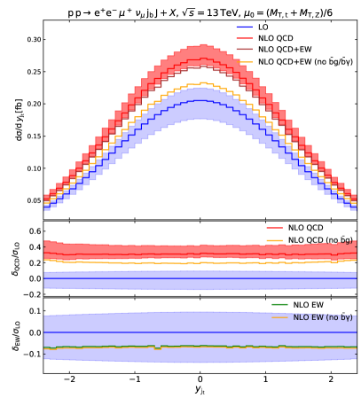
(a)

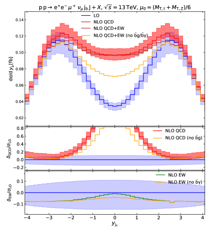
(b)

Figure 4: Rapidity distributions for the top-decay jet $\mathrm{j}_{\mathrm{b}}$ and spectator jet $\mathrm{j}_{s}$. See Sect. 2.4 for the definition of these objects.

Figure 4(a) presents the cross section differentially in the rapidity of the top-decay jet and Fig. 4(b) in the rapidity of the spectator jet, as defined in Sect. 2.4. The top-decay jet is mainly produced in the central region, $|y|<2$, whereas the behaviour of the spectator is determined by the $t$-channel W-boson propagator attached to the spectator quark line [see for example Fig. 1(a)] and therefore preferably produced in the forward region, peaking at $|y|\approx 2.5$, similar to the tagging jets in vector-boson scattering. At NLO QCD the two distributions are differently affected by the corrections: while the relative corrections are flat for the top-decay jet, they fill up the central region for the spectator jet, with a large contribution from the $\bar{}\text{b}\text{g}$ channels and an almost as large contribution from the bg channels. Extra gluon radiation from the spectator jet changes its direction filling effectively the central region, which is disfavoured at LO for the spectator jet. Moreover, the event reconstruction (see Sect. 2.4) enables to tag the gluon as the spectator jet, giving a rapidity spectrum which is in general more central than the one of the quark orginated from the $t$-channel topology. The EW corrections for the top-decay-jet rapidity distribution are practically constant and reproduce those of the integrated cross section. For the spectator jet, we observe a similar picture in the dominant region $|y|\gtrsim 2$, but smaller EW corrections in the central region in accordance with the results of the on-shell calculation Pagani:2020mov . The contribution of the $\bar{}\text{b}\gamma$ channels tends to cancel the EW corrections near $y_{{\rm j}_{\rm s}}\approx 0$.

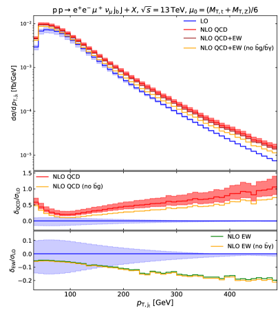
(a)

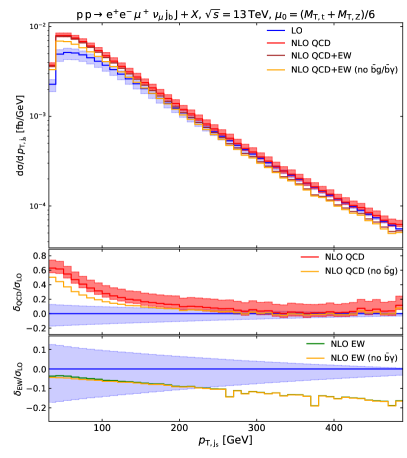
(b)

Figure 5: Transverse-momentum distributions for the top-decay jet $\mathrm{j}_{\mathrm{b}}$ and spectator jet $\mathrm{j}_{s}$.

The distributions of the transverse momenta of the top-decay jet and the spectator jet, presented in Figs. 5(a)–5(b), both receive $25\text{\,}\mathrm{\char 37\relax}60\text{\,}\mathrm{\char 37\relax}$ QCD corrections in the region $p_{{\mathrm{T}}}<$100\text{\,}\mathrm{GeV}$$. However, in the large-$p_{{\mathrm{T}}}$ regions the QCD corrections to the spectator-jet distribution approach zero, while those for the top-decay jet increase up to $100\text{\,}\mathrm{\char 37\relax}$. The striking difference between the two observables is due to the different LO behaviour, where the top-decay jet (resulting from the massive top quark) is much softer than the spectator jet (produced directly), while at NLO QCD the opening of the partonic channels with a gluon and a light quark ($\text{g}q$) in the initial state enhances the tail of both distributions. The LO behaviour is very similar to the one found in $t$–channel single-top production Frederix:2019ubd , where the spectator recoils against the top quark, and therefore the transverse momentum of the top quark (balancing the one of the spectator jet) is shared among its decay products, resulting in a top-decay jet with smaller $p_{{\mathrm{T}}}$ than the spectator jet. Since in tZj production the additional Z boson tends to be soft or closer in phase space to the top quark than to the spectator jet, the same argument applies explaining the relative softness of the top-decay jet. For both distributions in Fig. 5 the EW corrections grow negatively from roughly $-5\text{\,}\mathrm{\char 37\relax}-20\text{\,}\mathrm{\char 37\relax}$ in the large-$p_{\mathrm{T}}$ region. The relative EW corrections to the top-decay-jet transverse-momentum distribution are similar to those for the reconstructed top quark, showing in the tail the same Sudakov behaviour as in inclusive calculations (see Fig. 6 of Ref. Pagani:2020mov ). Our results for the relative EW corrections to the distribution in the transverse momentum of the spectator jet agree qualitatively with those for the transverse momentum of the leading light jet in Fig. 6 of Ref. Pagani:2020mov .

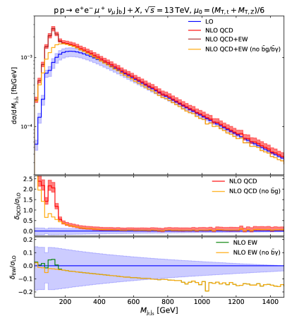
(a)

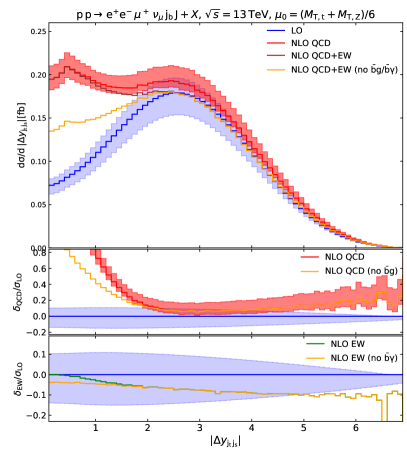
(b)

Figure 6: Invariant-mass and rapidity-separation distributions of the jet pair.

Looking at observables involving both the top-decay and spectator jet, we find a resonance in the invariant-mass distribution in Fig. 6(a) at around $M_{\mathrm{j}_{\mathrm{t}}\mathrm{j}_{s}}\approx$165\text{\,}\mathrm{GeV}$$. This resonance comes from an anti-top quark, which is produced starting from NLO QCD and EW in processes of the type given in Eq. (2) and decays hadronically, for example $\bar{\mathrm{t}}\to\bar{\mathrm{b}}\bar{\mathrm{u}}\mathrm{d}$ [see Fig. 2]. This contribution is clearly visible in the relative QCD and EW corrections. Since the two-jet invariant mass does not capture all three quarks of the anti-top decay—only when two of them are clustered together—the peak is below the top-quark mass. The EW corrections increase negatively up to $-15\text{\,}\mathrm{\char 37\relax}$ for invariant masses of $1500\text{\,}\mathrm{GeV}$. The QCD corrections diminish from $+25\%$ to $+10\%$ above $200\,\text{GeV}$.

In the distribution of the rapidity separation of the two jets, Fig. 6(b), we observe a rapidity gap of $|\Delta y_{\mathrm{j}_{\mathrm{t}}\mathrm{j}_{s}}|\approx 2.5$ at LO, as expected from the rapidities of the individual jets [see Figs. 4(a) and 4(b)]. At NLO QCD this gap is filled, which is consistent with the observation that strong corrections mostly affect the central regions of each jet distribution, as seen in rapidity spectra of individual jets [see Fig. 4(a)]. A large fraction of events for small $|\Delta y_{\mathrm{j}_{\mathrm{t}}\mathrm{j}_{s}}|$ originates from the $\bar{}\text{b}\text{g}$ anti-top production channels and the bg channels at NLO QCD. The corresponding $\bar{}\text{b}\gamma$ channels cancel the negative NLO EW corrections in the rapidity gap, which grow up to $-12\text{\,}\mathrm{\char 37\relax}$ for $|\Delta y_{\mathrm{j}_{\mathrm{t}}\mathrm{j}_{s}}|\approx 6$.

3.3.2 Leptonic observables

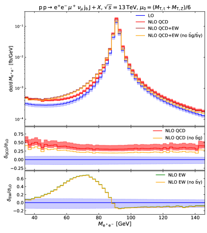
(a)

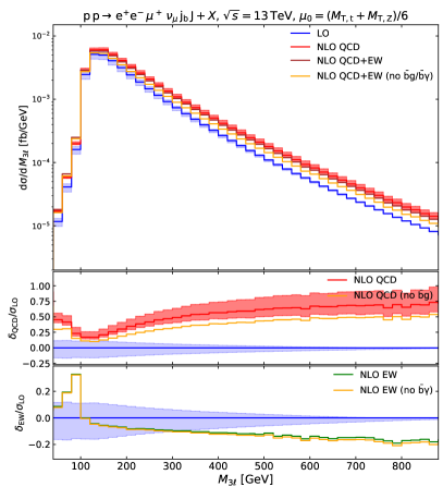
(b)

Figure 7: Invariant-mass distributions of the same-flavour lepton pair and of all three charged leptons.

Coming to leptonic observables, we see the Breit–Wigner shape from the Z-boson decay around its mass in the $M_{\mathrm{e}^{+}\mathrm{e}^{-}}$ distribution in Fig. 7(a). At NLO EW, soft-photon radiation causes positive corrections of up to $60\text{\,}\mathrm{\char 37\relax}$ below the Z-boson mass around $70\text{\,}\mathrm{GeV}$. This radiative return is very similar in terms of size and shape to Drell–Yan lepton-pair production. The NLO QCD corrections around the resonance are flat and reproduce those of the integrated cross section.

A similar effect of NLO EW corrections arises in the $M_{3\ell}$ observable in Fig. 7(b). The region below the peak is filled by events where a real photon emitted from one of the decay leptons is not included in $M_{3\ell}$, resulting in corrections of up to $35\text{\,}\mathrm{\char 37\relax}$. Negative NLO EW corrections of up to $-20\text{\,}\mathrm{\char 37\relax}$ arise for very large invariant masses. The NLO QCD corrections reach $70\%$ for small and large $M_{3\ell}$, while they are about $20\%$ near the peak of the distribution.

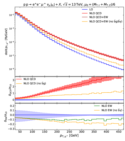
(a)

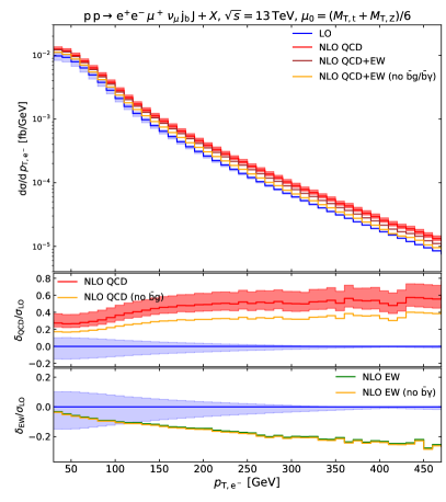
(b)

Figure 8: Transverse-momentum distributions of the anti-muon and the electron.

In Fig. 8 we show transverse-momentum distributions for the anti-muon and the electron. The EW corrections are comparably flat for the anti-muon due to the positive contribution of the $\bar{}\text{b}\gamma$ channels, cancelling most of the negative NLO EW corrections for large transverse momenta. For the electron transverse momentum, the NLO EW corrections grow negatively up to $-20\text{\,}\mathrm{\char 37\relax}$ around $500\,\text{GeV}$, suggesting the dominance of EW Sudakov logarithms. It is worth noticing that the anti-muon is a product of the decay of the top quark, while the electron comes from the decay of a Z boson, suggesting different behaviours in the enhancement of EW Sudakov logarithms of virtual origin. For what concerns QCD corrections, very different behaviours are found for the two charged leptons. The relative QCD corrections to the electron transverse-momentum distribution increase from $25\%$ to $50\%$ in the moderate-$p_{{\mathrm{T}}}$ region and flatten out for values larger than $200\,\text{GeV}$. The transverse-momentum distribution of the anti-muon is much stronger affected by QCD corrections, which enhance the LO distribution by up to $400\%$. This huge effect can be explained with polarisation arguments. At LO the $\text{W}^{+}$ bosons (decaying into $\mu^{+}\nu_{\mu}$) mostly come from the top-quark decay and are therefore either longitudinal (dominant) or left handed (subdominant). As a consequence the anti-muons resulting from the W decays are preferably emitted in the direction opposite to the high-energetic $\text{W}^{+}$ boson and therefore have softer $p_{{\mathrm{T}}}$. At NLO QCD the large anti-top contribution in the $\bar{\text{b}}\text{g}$ channel is characterised by $\text{W}^{+}$ bosons that are preferably right handed (as they originate from the anti-top quark via a helicity-right-handed coupling) leading to emitted anti-muons collinear to the $\text{W}^{+}$ bosons and therefore enhancing the high-$p_{{\mathrm{T}}}$ tail.

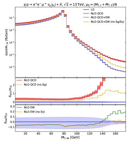
(a)

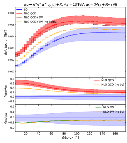
(b)

Figure 9: Transverse-mass distribution of the W boson as defined in Eq. (26) and azimuthal-angle-separation distribution of the $\text{e}^{+}\text{e}^{-}$ pair.

In Fig. 9(a) we present the distribution in the transverse mass of the W boson, defined as

$$M_{\mathrm{T}}^{\mathrm{W}}=\sqrt{2p_{\mathrm{T}}^{\mu^{+}}p_{\mathrm{T},\text{miss}}(1-\cos\Delta\phi_{\mu^{+}\text{miss}})}\text{,}$$ (26)

where $p_{\mathrm{T},\text{miss}}$ is the missing transverse momentum and $\Delta\phi_{\mu^{+}\text{miss}}$ the azimuthal angle between the transverse momentum of the anti-muon and the missing transverse momentum. This distribution is very similar to the one measured in the charge-current Drell–Yan process with the characteristic edge at around $M_{\mathrm{W}}$. The NLO QCD and EW corrections are flat in a region up to $100\text{\,}\mathrm{GeV}$, after which they increase mainly due to the anti-top production channels $\bar{}\text{b}\text{g}/\bar{}\text{b}\gamma$, in which the charged-lepton–neutrino pair is not produced in a top-quark decay. While contributions with a (transverse) mass of the W boson above the top-quark mass cannot contain a resonant top quark, they can still contain a resonant anti-top quark.

Figure 9(b) displays the cross section differentially in the azimuthal angle between the $\text{e}^{+}\text{e}^{-}$ pair. At LO the electron and positron are more likely to be back-to-back ($\Delta\phi_{\mathrm{e}^{-}\mathrm{e}^{+}}>$90\text{\,}\mathrm{\SIUnitSymbolDegree}$$) than along each other ($\Delta\phi_{\mathrm{e}^{-}\mathrm{e}^{+}}<$90\text{\,}\mathrm{\SIUnitSymbolDegree}$$). The NLO EW corrections vary from $-10\text{\,}\mathrm{\char 37\relax}-5\text{\,}\mathrm{\char 37\relax}$. At NLO QCD, the corrections are larger for lepton pairs close to each other in the azimuthal plane, which typically result from high-energetic Z bosons, and smaller for the back-to-back configuration.

3.3.3 Lepton–jet observables

Figure 10(a) shows the distribution of the cross section in the invariant mass of the top-decay jet and the anti-muon, which peaks at $M_{\mathrm{j}_{\mathrm{t}}\mu^{+}}\approx$120\text{\,}\mathrm{GeV}$$ and $M_{\mathrm{j}_{\mathrm{t}}\mu^{+}}\approx$110\text{\,}\mathrm{GeV}$$ in LO and NLO QCD, respectively, displaying a sharp drop around $M_{\mathrm{j}_{\mathrm{t}}\mu^{+}}=\sqrt{M_{\mathrm{t}}^{2}-M_{\mathrm{W}}^{2}}\approx$153\text{\,}\mathrm{GeV}$$, the threshold for having both an on-shell top quark and W boson.

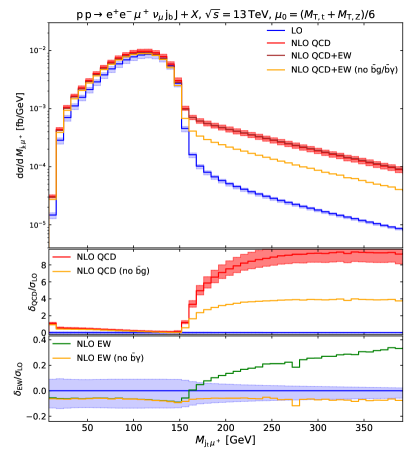
(a)

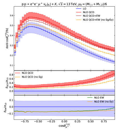
(b)

Figure 10: Invariant-mass distribution of the top-decay jet and the anti-muon, and distribution of the cosine of the angle of the anti-muon with respect to the direction of the boost from the laboratory frame to the top-quark rest frame in the latter frame. The definition of the angle, given in Eq. (27), makes uses of the kinematic reconstruction routine given in Sect. 2.4.

Above this threshold, we find large corrections owing to off-shell top-quark production and the $\bar{}\text{b}\text{g}/\bar{}\text{b}\gamma$ anti-top production channels (both in NLO QCD and NLO EW), in which the W boson is not part of the top-quark decay.

Finally, in Fig. 10(b), we present the distribution in the cosine of the decay angle of the anti-muon in the top-quark rest frame. This angle is defined as the angular separation between the anti-muon momentum in the top-quark rest frame, $\vec{p}^{\,*}_{\mu^{+}}$, and the direction of the boost from the laboratory frame to the top-quark rest frame, $\vec{n}^{*}_{\mathrm{t}}$, (top-quark momentum in the laboratory frame)

$$\cos\theta_{\mu^{+}}^{\,*(\mathrm{t})}=\frac{\vec{p}^{\,*}_{\mu^{+}}\cdot\vec{n}^{*}_{\mathrm{t}}}{|\vec{p}^{\,*}_{\mu^{+}}||\vec{n}^{*}_{\mathrm{t}}|}\,,$$ (27)

where the top-quark momentum is reconstructed with the procedure detailed in Sect. 2.4. This observable is highly sensitive to the helicity of the top quark. In the absence of radiative corrections and of cuts on the decay products, the (normalised) top-quark decay rate for $\text{t}\rightarrow\text{b}\ell^{+}\nu_{\ell}$ reads

$$\frac{1}{\sigma}\frac{\mathrm{d}\sigma}{\mathrm{d}\cos\theta^{*(\text{t})}_{\ell^{+}}}=\frac{1}{2}\left(1+\kappa_{\ell^{+}}(f_{+}-f_{-})\cos\theta^{*(\text{t})}_{\ell^{+}}\right)\,,$$ (28)

where $\kappa_{\ell^{+}}$ (=1 in the SM) is the spin analyser of the charged lepton and therefore sensitive to anomalous tWb couplings Jezabek:1994zv ; Aguilar-Saavedra:2006qvv ; Aguilar-Saavedra:2014eqa , while $f_{+}$, $f_{-}$ are the right- and left-helicity fractions dictated by the dynamics of the top-quark production. Due to the intrinsic frame dependence of helicity, different choices are possible for the quantisation axis for the top-quark spin Mahlon:1999gz ; Schwienhorst:2010je ; Aguilar-Saavedra:2012bvs . In single-top-production studies usual choices are the so-called helicity basis Jezabek:1994zv ; Schwienhorst:2010je and the spectator basis Mahlon:1999gz ; Schwienhorst:2010je ; Aguilar-Saavedra:2014eqa . The angle defined in Eq. (27) probes top-quark helicities defined with respect to the direction of the boost from the laboratory frame to the top-quark rest frame, which is a simple choice at the LHC and gives similar results as the helicity basis Schwienhorst:2010je . Although used in experimental analyses CMS:2021ugv , the spectator-basis (helicities defined with the spectator-jet direction as reference axis) is a less natural choice in the presence of an additional Z boson that recoils against the system formed by the top quark and the spectator jet.

Even though the shape expected from Eq. (28) is distorted by fiducial cuts and kinematic reconstruction of the top quark, resulting in the depletion of the anti-collinear region, the LO distribution shown in the top panel of Fig. 10(b) clearly shows a strong left-handed polarisation of the top quark. The NLO QCD corrections increase towards large $\cos\theta^{*(\text{t})}_{\mu^{+}}$, with large contributions from gluon-induced partonic channels, suggesting spin configurations in the real corrections that favour a right-handed top quark. The EW corrections are flat for $\cos\theta^{*(\text{t})}_{\mu^{+}}\lesssim 0.5$ but are reduced for larger values of $\cos\theta^{*(\text{t})}_{\mu^{+}}$ in particular also owing to contributions of the $\bar{}\text{b}\gamma$ channels.

4 Conclusions

We have presented a calculation of NLO EW and QCD corrections to off-shell tZj production at the LHC. All effects of non-resonant top-quark or Z-boson contributions and full spin correlations are accounted for both at LO and at NLO. A realistic fiducial phase-space region is considered for the Monte Carlo predictions of integrated and differential cross sections.

At integrated level, the NLO QCD and EW corrections amount to $+31\%$ and $-7\%$, respectively, of the LO fiducial cross section. In more exclusive and off-shell regions, the NLO QCD effects become of order $+100\%$ and larger and generate strong shape distortions of LO distributions. The NLO EW corrections reach the order of $-20\%$ in the tails of several transverse-momentum distributions.

The considered inclusive fiducial volume enables the opening of partonic channels embedding a $\bar{\text{t}}\text{W}\text{Z}$ resonance structure at NLO which gives a sizeable enhancement to the LO cross section ($+12\%$ at integrated level). Vetoes on additional jets and kinematic constraints may be considered in experimental analyses to suppress this background.

The top-quark-decay effects with full off-shell matrix elements, so far missing in the literature, represent a necessary ingredient for the complete fixed-order (NLO) modelling of tZj production in the SM. Therefore the results shown in this work will be relevant for upcoming LHC differential measurements of this process.

References

- (1) G. Mahlon and S. J. Parke, Single top quark production at the LHC: Understanding spin, Phys. Lett. B 476 (2000) 323–330, [hep-ph/9912458].
- (2) CMS Collaboration, A. M. Sirunyan et al., Measurement of the associated production of a single top quark and a Z boson in pp collisions at 13 TeV, Phys. Lett. B 779 (2018) 358–384, [arXiv:1712.02825].
- (3) ATLAS Collaboration, M. Aaboud et al., Measurement of the production cross-section of a single top quark in association with a Z boson in proton–proton collisions at 13 TeV with the ATLAS detector, Phys. Lett. B 780 (2018) 557–577, [arXiv:1710.03659].
- (4) CMS Collaboration, A. M. Sirunyan et al., Observation of Single Top Quark Production in Association with a Boson in Proton-Proton Collisions at =13 TeV, Phys. Rev. Lett. 122 (2019) 132003, [arXiv:1812.05900].
- (5) ATLAS Collaboration, G. Aad et al., Observation of the associated production of a top quark and a boson in collisions at 13 TeV with the ATLAS detector, JHEP 07 (2020) 124, [arXiv:2002.07546].
- (6) CMS Collaboration, A. Tumasyan et al., Inclusive and differential cross section measurements of single top quark production in association with a Z boson in proton-proton collisions at = 13 TeV, JHEP 02 (2022) 107, [arXiv:2111.02860].
- (7) C. Degrande, F. Maltoni, K. Mimasu, E. Vryonidou, and C. Zhang, Single-top associated production with a or boson at the LHC: the SMEFT interpretation, JHEP 10 (2018) 005, [arXiv:1804.07773].
- (8) J. Campbell, R. K. Ellis, and R. Röntsch, Single top production in association with a Z boson at the LHC, Phys. Rev. D 87 (2013) 114006, [arXiv:1302.3856].
- (9) D. Pagani, I. Tsinikos, and E. Vryonidou, NLO QCD+EW predictions for and production at the LHC, JHEP 08 (2020) 082, [arXiv:2006.10086].
- (10) J. Campbell, T. Neumann, and Z. Sullivan, Testing parton distribution functions with t-channel single-top-quark production, Phys. Rev. D 104 (2021) 094042, [arXiv:2109.10448].
- (11) J. Reuter and M. Tonini, Top Partner Discovery in the T tZ channel at the LHC, JHEP 01 (2015) 088, [arXiv:1409.6962].
- (12) B. H. Li, Y. Zhang, C. S. Li, J. Gao, and H. X. Zhu, Next-to-leading order QCD corrections to associated production via the flavor-changing neutral-current couplings at hadron colliders, Phys. Rev. D 83 (2011) 114049, [arXiv:1103.5122].
- (13) N. Kidonakis, Higher-order corrections for production via anomalous couplings, Phys. Rev. D 97 (2018) 034028, [arXiv:1712.01144].
- (14) Y.-B. Liu and S. Moretti, Probing tqZ anomalous couplings in the trilepton signal at the HL-LHC, HE-LHC and FCC-hh, Chin. Phys. C 45 (2021) 043110, [arXiv:2010.05148].
- (15) R. K. Barman and A. Ismail, Constraining the top electroweak sector of the SMEFT through associated top pair and single top production at the HL-LHC, arXiv:2205.07912.
- (16) P. Falgari, F. Giannuzzi, P. Mellor, and A. Signer, Off-shell effects for t-channel and s-channel single-top production at NLO in QCD, Phys. Rev. D 83 (2011) 094013, [arXiv:1102.5267].
- (17) R. Frederix, D. Pagani, and I. Tsinikos, Precise predictions for single-top production: the impact of EW corrections and QCD shower on the -channel signature, JHEP 09 (2019) 122, [arXiv:1907.12586].
- (18) A. Banfi, G. P. Salam, and G. Zanderighi, Infrared safe definition of jet flavor, Eur. Phys. J. C 47 (2006) 113–124, [hep-ph/0601139].
- (19) A. Denner and R. Feger, NLO QCD corrections to off-shell top-antitop production with leptonic decays in association with a Higgs boson at the LHC, JHEP 11 (2015) 209, [arXiv:1506.07448].
- (20) A. Denner and M. Pellen, NLO electroweak corrections to off-shell top-antitop production with leptonic decays at the LHC, JHEP 08 (2016) 155, [arXiv:1607.05571].
- (21) A. Denner, J.-N. Lang, M. Pellen, and S. Uccirati, Higgs production in association with off-shell top-antitop pairs at NLO EW and QCD at the LHC, JHEP 02 (2017) 053, [arXiv:1612.07138].
- (22) A. Denner and M. Pellen, Off-shell production of top-antitop pairs in the lepton+jets channel at NLO QCD, JHEP 02 (2018) 013, [arXiv:1711.10359].
- (23) A. Denner and G. Pelliccioli, NLO QCD corrections to off-shell production at the LHC, JHEP 11 (2020) 069, [arXiv:2007.12089].
- (24) A. Denner and G. Pelliccioli, Combined NLO EW and QCD corrections to off-shell production at the LHC, Eur. Phys. J. C 81 (2021) 354, [arXiv:2102.03246].
- (25) S. Actis, A. Denner, L. Hofer, A. Scharf, and S. Uccirati, Recursive generation of one-loop amplitudes in the Standard Model, JHEP 04 (2013) 037, [arXiv:1211.6316].
- (26) S. Actis, et al., RECOLA: REcursive Computation of One-Loop Amplitudes, Comput. Phys. Commun. 214 (2017) 140–173, [arXiv:1605.01090].
- (27) A. Denner, S. Dittmaier, and L. Hofer, COLLIER: a fortran-based Complex One-Loop LIbrary in Extended Regularizations, Comput. Phys. Commun. 212 (2017) 220–238, [arXiv:1604.06792].
- (28) A. Denner and S. Dittmaier, Reduction of one-loop tensor 5-point integrals, Nucl. Phys. B 658 (2003) 175–202, [hep-ph/0212259].
- (29) A. Denner and S. Dittmaier, Reduction schemes for one-loop tensor integrals, Nucl. Phys. B 734 (2006) 62–115, [hep-ph/0509141].
- (30) A. Denner and S. Dittmaier, Scalar one-loop 4-point integrals, Nucl. Phys. B 844 (2011) 199–242, [arXiv:1005.2076].
- (31) S. Catani and M. Seymour, A general algorithm for calculating jet cross-sections in NLO QCD, Nucl. Phys. B 485 (1997) 291–419, [hep-ph/9605323]. [Erratum: Nucl. Phys. B 510 (1998) 503–504].
- (32) S. Dittmaier, A general approach to photon radiation off fermions, Nucl. Phys. B 565 (2000) 69–122, [hep-ph/9904440].
- (33) S. Catani, S. Dittmaier, M. H. Seymour, and Z. Trócsányi, The dipole formalism for next-to-leading order QCD calculations with massive partons, Nucl. Phys. B 627 (2002) 189–265, [hep-ph/0201036].
- (34) S. Dittmaier, A. Kabelschacht, and T. Kasprzik, Polarized QED splittings of massive fermions and dipole subtraction for non-collinear-safe observables, Nucl. Phys. B800 (2008) 146–189, [arXiv:0802.1405].
- (35) A. Denner, S. Dittmaier, P. Maierhöfer, M. Pellen, and C. Schwan, QCD and electroweak corrections to WZ scattering at the LHC, JHEP 06 (2019) 067, [arXiv:1904.00882].
- (36) Particle Data Group Collaboration, P. A. Zyla et al., Review of Particle Physics, PTEP 2020 (2020) 083C01.
- (37) D. Yu. Bardin, A. Leike, T. Riemann, and M. Sachwitz, Energy-dependent width effects in annihilation near the Z-boson pole, Phys. Lett. B206 (1988) 539–542.
- (38) L. Basso, S. Dittmaier, A. Huss, and L. Oggero, Techniques for the treatment of IR divergences in decay processes at NLO and application to the top-quark decay, Eur. Phys. J. C76 (2016) 56, [arXiv:1507.04676].
- (39) M. Jeżabek and J. H. Kühn, QCD Corrections to Semileptonic Decays of Heavy Quarks, Nucl. Phys. B314 (1989) 1–6.
- (40) A. Denner, S. Dittmaier, M. Roth, and D. Wackeroth, Electroweak radiative corrections to fermions in double pole approximation: The RACOONWW approach, Nucl. Phys. B587 (2000) 67–117, [hep-ph/0006307].
- (41) A. Denner, S. Dittmaier, M. Roth, and D. Wackeroth, Predictions for all processes , Nucl. Phys. B560 (1999) 33–65, [hep-ph/9904472].
- (42) A. Denner, S. Dittmaier, M. Roth, and L. H. Wieders, Electroweak corrections to charged-current fermion processes: Technical details and further results, Nucl. Phys. B724 (2005) 247–294, [hep-ph/0505042]. [Erratum: Nucl. Phys. B 854 (2012) 504].
- (43) A. Denner and S. Dittmaier, The complex-mass scheme for perturbative calculations with unstable particles, Nucl. Phys. B Proc. Suppl. 160 (2006) 22–26, [hep-ph/0605312].
- (44) A. Denner and S. Dittmaier, Electroweak Radiative Corrections for Collider Physics, Phys. Rept. 864 (2020) 1–163, [arXiv:1912.06823].
- (45) A. Buckley, et al., LHAPDF6: parton density access in the LHC precision era, Eur. Phys. J. C 75 (2015) 132, [arXiv:1412.7420].
- (46) NNPDF Collaboration, V. Bertone, S. Carrazza, N. P. Hartland, and J. Rojo, Illuminating the photon content of the proton within a global PDF analysis, SciPost Phys. 5 (2018) 008, [arXiv:1712.07053].
- (47) S. Catani, Y. L. Dokshitzer, M. Olsson, G. Turnock, and B. R. Webber, New clustering algorithm for multi-jet cross-sections in annihilation, Phys. Lett. B 269 (1991) 432–438.
- (48) S. Catani, Y. L. Dokshitzer, M. H. Seymour, and B. R. Webber, Longitudinally invariant clustering algorithms for hadron hadron collisions, Nucl. Phys. B 406 (1993) 187–224.
- (49) S. D. Ellis and D. E. Soper, Successive combination jet algorithm for hadron collisions, Phys. Rev. D 48 (1993) 3160–3166, [hep-ph/9305266].
- (50) M. Czakon, A. Mitov, and R. Poncelet, Infrared-safe flavoured anti- jets, arXiv:2205.11879.
- (51) R. Gauld, A. Huss, and G. Stagnitto, A dress of flavour to suit any jet, arXiv:2208.11138.
- (52) Q.-H. Cao, R. Schwienhorst, J. A. Benitez, R. Brock, and C. P. Yuan, Next-to-leading order corrections to single top quark production and decay at the Tevatron: 2. -channel process, Phys. Rev. D 72 (2005) 094027, [hep-ph/0504230].
- (53) R. Schwienhorst, C. P. Yuan, C. Mueller, and Q.-H. Cao, Single top quark production and decay in the -channel at next-to-leading order at the LHC, Phys. Rev. D 83 (2011) 034019, [arXiv:1012.5132].
- (54) F. Demartin, F. Maltoni, K. Mawatari, and M. Zaro, Higgs production in association with a single top quark at the LHC, Eur. Phys. J. C 75 (2015) 267, [arXiv:1504.00611].
- (55) M. Jezabek and J. H. Kühn, V-A tests through leptons from polarized top quarks, Phys. Lett. B 329 (1994) 317–324, [hep-ph/9403366].
- (56) J. A. Aguilar-Saavedra, J. Carvalho, N. F. Castro, F. Veloso, and A. Onofre, Probing anomalous Wtb couplings in top pair decays, Eur. Phys. J. C 50 (2007) 519–533, [hep-ph/0605190].
- (57) J. A. Aguilar-Saavedra and S. Amor Dos Santos, New directions for top quark polarization in the -channel process, Phys. Rev. D 89 (2014) 114009, [arXiv:1404.1585].
- (58) J. A. Aguilar-Saavedra and R. V. Herrero-Hahn, Model-independent measurement of the top quark polarisation, Phys. Lett. B 718 (2013) 983–987, [arXiv:1208.6006].