Oscillation tomografy study of Earth’s composition and density with atmospheric neutrinos

Abstract

Knowledge of the composition of the Earth’s interior is highly relevant to many geophysical and geochemical problems. Neutrino oscillations are modified in a non-trivial way by the matter effects and can provide valuable and unique information not only on the density but also on the chemical and isotopic composition of the deep regions of the planet. In this paper, we re-examine the possibility of performing an oscillation tomography of the Earth with atmospheric neutrinos and antineutrinos to obtain information on the composition and density of the outer core and the mantle, complementary to that obtained by geophysical methods. Particular attention is paid to the D^′′ layer just above the core-mantle boundary and to the water (hydrogen) content in the mantle transition zone. Our analysis is based on a Monte-Carlo simulation of the energy and azimuthal angle distribution of $\mu$-like events generated by neutrinos. Taking as reference a model of the Earth consisting of 55 concentric layers with constant densities determined from the PREM, we evaluate the effect on the number of events due to changes in the composition and density of the outer core and the mantle. To examine the capacity of a detector like ORCA to resolve such variations, we construct regions in planes of two of these quantities where the statistical significance of the discrepancies between the reference and the modified Earth are less than $1\sigma$. The variations are implemented in such a way that the constraint imposed by both the total mass of the Earth and its moment of inertia are verified.

1 Introduction

Aside from its intrinsic interest, a detailed description of the inner parts of the Earth is essential for a proper understanding of basic geological phenomena such as volcanology, earthquakes, plate tectonics, and mountain building tarbuck2009earth ; fowler:2005 . According to current knowledge, the Earth’s internal structure is stratified and consist of successive layers with different chemical, geological, and physical properties. Most of the information about the layers and the boundaries between them has been acquired by examining how seismic waves created by natural earthquakes are refracted and reflected as they propagate through the Earth Lay:1995 ; Aki:2002 . Valuable information has also been obtained from measurements of magnetic and gravitational fields, observations of the planet’s moment of inertia and precessional motion, and physical, chemical, and mineralogical analyzes of meteorites and xenoliths. Based on chemical composition, three main layers have been identified within our planet: the crust, the mantle, and the core. The mantle and the core are further subdivided into two regions each.

The mantle surrounds the core and extends from beneath the thin crust to a depth of 2,900 km. It consists mainly of dense silicate rocks rich in iron and magnesium. Seismic wave velocities in the mantle show three discontinuities at depths of 410, 660 and 2,700 km Helffrich:2001 . The first two correspond to the edges of the transition zone between the upper and lower mantle, and are best explained by mineral phase transformations without compositional changes. The third discontinuity is typically a 2.5-3.0% increase for both S- and P-waves observed at the top of the D^′′ layer, a transition shell about 200-300 km thick, at the base of the mantle, which presents a variety of seismic anomalies and is presumably the source of the large mantle plumes Loper:1995 ; Laywg:1998 . This layer is not yet fully understood, many of its characteristic may be attributed to the discovered MgSi${\rm O}_{3}$ postperovskite phase Murakami:2004 , but compositional differences may also play an important role in addition to the phase transformation Hiroshe:2021 . Regarding the core, it is well established that it is composed primarily of an iron-nickel alloy, with Ni/Fe $\sim 0.06$. The inner core is solid, while the lower density and absence of S-wave propagation are indications of a liquid outer core. The density deficit in the outer core cannot be simply explained by a difference in the state, but it requires about 5-10 wt% (weight percent) of lower atomic weight elements to reduce its density and melting point Birch:1964 ; Poirier:1994 .

Good estimates of the abundance and distribution of “light” elements in the core are essential to understanding the formation and evolution of the Earth, as well as how the core and mantle interact in the region around the core-mantle boundary (CMB) Litasov:2016 ; Hiroshe:2021 . The various processes that occur in this interface are highly influenced by heterogeneous structures at or near it. The great disparity in density prevents direct convection movement through the CMB, and nearby regions control the transfer of heat and material Wookey:2008 . These processes strongly affect the convection in the mantle, responsible for the plate motion and continental drift, and the more vigorous convective flow in the outer core that is believed to be at the origin of the Earth’s magnetic field (i.e., the functioning of the geodynamo) Lister:1995 ; Roberts:2013 . Due to vigorous convection, the liquid part of the core is usually assumed to have a uniform composition. However, seismological evidence indicates the possible existence of a $\sim 300$ km thick region on top of the outer core (E^′ layer), which shows anomalous low seismic velocities. This region is likely to be less dense than the rest of the outer core, but simply increasing the concentration of light elements also produces higher speeds, in contradiction with observations. None of the mechanisms that have been considered are without complications Brodholt:2017 and further observations are needed before a satisfactory explanation of the origin and nature of the E’ layer can be formulated.

The study of seismic wave propagation and normal mode oscillation is undoubtedly the most effective and reliable method to search the Earth’s deep structures and process. Nevertheless, the impressive progress done has not been accompanied with a concomitant improvement in the precision of the density estimations Bolt:1995 . They are done through an underdetermined inversion problem, performed in two steps: the spatial distribution of seismic wave velocities is first inferred from seismological data and then the density distribution is inferred from the seismic velocities using some empirical relation Geller:2003 . Such procedure allows the average density along a path to be estimated with an uncertainties of about 5% Bolt:1995 for the mantle and presumably larger for the core. For example, the density jump at the inner-core boundary, which play an important role in the maintenance of the geodynamo, has been inferred to be of 0.82 with an error of more than 20% Master:2003 . While the density distribution can be obtained from seismological remote sensing, the compositional structure of the Earth McDonough:1995 ; allegre1995chemical has been much more difficult to determine. Thus, the compositions of the lower mantle and the core remain quite uncertain, despite significant advances in recent years. Since in situ sampling is impossible, estimations are done by comparing density and sound velocity data from seismological observations with those from laboratory experiments and theoretical calculations Zhang:2016 . Due to technical limitations, it has been difficult to perform reliable experiments for molten samples under high pressure and temperature conditions and the available information is still insufficient to infer the core composition. The most likely light elements in the core are oxygen, silicon, carbon, nitrogen, sulfur, and hydrogen Li:2021 ; Hiroshe:2021 , but there is still no consensus on the nature and proportion of the components.

In addition to the metallic core, significant amounts of hydrogen can be incorporated within the mantle, in silicate minerals, melts, and hydrous fluids. This is done in a variety of chemical species (OH, H₂, $\cdots$) generically referred to as “water" Hirschmann:2006 ; Peslier:2017 ; Othani:2020 . The abundance and distribution of water has influenced not only the evolution, dynamics state and thermal structure of the deep interior, but also the evolution of the crust and hydrosphere Bodnar:2013 . Even small amount of water can affect properties like melting temperature, rheological properties, electrical conductivity, and seismic velocities of the mantle. How water is transported into Earth’s deep interior and how it is distributed are today open questions. Almost no constraints exists on the water content of the lower mantle. The existing laboratory data cannot be used to infer the water content from geophysical observations at these high pressure and temperature conditions. Low-velocity regions have been observed near the top of the lower mantle and directly above the CMB Peslier:2017 . If the low-velocity is interpreted as caused by partial melting, then some water is likely be present in these regions Garnero:2016 . Water could instead be stored in the lowest parts of the mantle in Al-postperovskite Townsend:2016 . There is a wide consensus that the mantle transition zone (MTZ), at 410-660 km deep, is a potential reservoir of water because its main mineral constituents can store up to $\sim 3\%$ wt water Bodnar:2013 . However, the amount of water contained there is poorly constrained. Some water-rich inclusions recently found in diamonds Pearson:2014 ; tschauner2018ice suggest a wet MTZ, but it is not clear if they are representative of the typical water content of the deep mantle or reflect local conditions. Geophysical methods (electrical conductivity and seismic observations) provides constraints on the water distribution in a global scale karato2011water . The inferences with these approaches are not direct and, despite the effort involved, a wide range of values have been reported in the literature karato:2020 ; Fei:2017 . As noticed in Ref. karato:2020 , geophysical estimates have large uncertainties and the water content in the MTZ can be heterogeneous, having significant lateral variability as revealed by a recent novel approach munch:2020 .

From the comments in the previous paragraph it is apparent how useful it would be to have additional experimental techniques, unaffected by the same uncertainties, which could provide complementary and independent information about the deep interior of the Earth. A promising candidate is neutrino tomography Winter:2006vg . The basic idea is that neutrino propagation within the Earth is affected by their interactions with the particles present in the terrestrial matter. The cross section for neutrino interactions increase with energy and, in the case of absorption tomography, the density profile can be reconstructed from the attenuation of the flux of very high energy ($\gtrsim 10$ TeV) neutrinos passing through the Earth Volkova:1974xa ; Wilson:1983an ; Ralston:1999fz ; Jain:1999kp ; GonzalezGarcia:2007gg ; Reynoso:2004dt ; Romero:2011zzb ; Donini:2018tsg . Another option is oscillation tomography, which takes advantage of the matter effect on flavor oscillations Wolfenstein:1977ue ; Barger:1980tf ; Mikheev:1986gs of lower energy (MeV to GeV) neutrinos. In a medium, the transition probabilities between active neutrinos depend on the number density of electrons $n_{e}$ along the neutrino trajectory, which is proportional to the product of the matter density $\rho$ times the average ratio $Z/A$ of the atomic number $Z$ and the mass number $A$ Nicolaidis:1987fe ; Nicolaidis:1990jm ; Winter:2006vg ; Borriello:2009ad ; Winter:2015zwx ; Rott:2015kwa ; VanElewyck:2017dga ; Bourret:2017tkw ; DOlivo:2020ssf ; Kelly:2021jfs ; Denton:2021rgt ; Upadhyay:2021kzf .

In this paper, we re-examine the feasibility of studying the internal structure of the Earth using atmospheric neutrino oscillation tomography. We analyze the ability of a detector such as ORCA to resolve deviations both of density and composition with respect to a standard Earth modeled in terms of 55 concentric shells integrated in five main layers, corresponding to the inner and outer core, the lower and upper mantle, and the crust. Constant densities are assigned to the shells from the mean value of the PREM densities within each shell. In our scheme, unlike other work on the subject, the densities of the main layers can be modified in a manner consistent with the well-measured total mass and moment of inertia of the Earth. In contrast, $Z/A$ is a function of the chemical and isotopic composition of the medium and is not subject to either of these constraints. Therefore, in principle, one could constrain the allowed values of the density and composition of the Earth’s deeper regions by studying the effects that changes in these quantities have on the events produced by atmospheric neutrinos after traversing the Earth, holding the total mass and moment of inertia of the planet fixed. We focus on the possible application to obtain information on the composition and density of the lower mantle regions above the CMB, in particular, the D^′′ region, paying special attention to the content of light elements, more specifically hydrogen. With the exception of hydrogen ($(Z/A)_{H}=1$), all other light elements have an almost equal number of protons and neutrons and hence $Z/A\cong 0.5$ for them. Thus, the presence of a significant amount of hydrogen (water) would produce appreciable $Z/A$ changes compared to those in dry regions. In this sense, information from neutrino oscillation tomography could give valuable information on the water content in the lower mantle and core. We also allow for some variation in the location of the boundary between the lower and upper mantle as an effective way to account for the transition region between these two layers.

The paper is organized as follows. In Sect. 2 we present a model of the Earth’s structure with 55 shells integrated within 5 main layers. In Sect. 3 we briefly review the formalism of matter neutrino oscillations and describe the algorithm to calculate the transition probabilities. In Sect. 4 we determine the number of $\mu$-like neutrino events in a detector such as ORCA and the effects that changes in the composition and density of the outer core and lower mantle have on this observable. The results and final comments are presented in Sect.5, where we carry out a Monte Carlo simulation of the number of $\mu$-like events and apply it to test different composition models of the outer core and mantle, changing also the density.

2 Model of the Earth’s structure

The observed lateral variations in the Earth’s properties are much less pronounced than the vertical variations. Therefore, the internal structure of the Earth can be well approximated by one-dimensional spherically symmetric models of seismic velocities, attenuation, and density as a function of depth dziewonski1981preliminary ; Kennett:1995 .The most widely used of these models for seismic tomography has been the Preliminary Reference Earth Model (PREM) dziewonski1981preliminary . This model represents the mean properties of the Earth as a function of the radial distance $r$ and was designed to fit different data sets and some basic data of the planet (radius, mass, and moment of inertia). In this study, we use a spherical model consisting of 55 concentric shells, each with a constant density equal to the average value of the PREM densities in the shell. The set of shells is divided into five large layers demarcated by concentric spheres of different radii: inner core ($IC$), outer core ($OC$), lower mantle ($M_{1}$), upper mantle ($M_{2}$), and crust ($C$). In Table 1 we give the values for the standard composition and the corresponding radii.

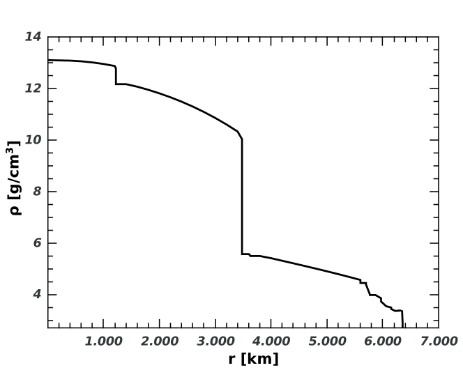
Figure 1: PREM density profile of the Earth with 55 shells.

Layer	$n^{0}$ of Shells	$R_{inf}$ - $R_{sup}$ [km]	Z/A
Inner Core	7	0 - 1221.5	0.4691
Outer Core	13	1221.5 - 3480	0.4691
Lower Mantle	$N_{M_{1}}$-$21$	$3480$ - $R_{M_{1}}$	0.4954
Upper Mantle	$49$-$N_{M_{1}}$	$R_{M_{1}}$ - $6346$	0.4954
Crust	6346-6371	6346 - 6371	0.4956

Table 1: Compositions of the main Earth layers.

The primary information on the Earth’s density as a function of $r$ comes from the total mass of the Earth $M_{{}_{\oplus}}=5.9724\times 10^{27}{\rm g}$ and its mean moment of inertia about the polar axis $I_{{}_{\oplus}}=8.025\times 10^{44}{\rm g}\hskip 0.85355pt{\rm cm}^{2}$ Williams:1994 . From these two quantities and $R_{{}_{\oplus}}=6371$ km for the Earth’s radius, one gets $I_{{}_{\oplus}}\simeq 0.33M_{{}_{\oplus}}R^{2}_{{}_{\oplus}}$ that is noticeably smaller than the moment of inertia of a homogeneous sphere of the same radius ($0.40M_{{}_{\oplus}}R^{2}_{{}_{\oplus}}$). This corroborates that there must be a concentration of mass towards the center of the planet or, in other words, that the inner regions are denser than average. We require that our model satisfy both constraints:

$$M_{{}_{\oplus}} = \frac{4}{3}\pi\sum_{i=1}^{55}\rho_{i}(R_{i+1}^{3}-R_{i}^{3})=M_{{\scriptscriptstyle IC}}+M_{{\scriptscriptstyle OC}}+M_{M_{1}}+M_{M_{2}}+M_{C}$$

$$I_{{}_{\oplus}} = \frac{8}{15}\pi\sum_{i=1}^{55}\rho_{i}(R_{i+1}^{5}-R_{i}^{5})=I_{{\scriptscriptstyle IC}}+I_{{\scriptscriptstyle OC}}+I_{M_{1}}+I_{M_{2}}+I_{C}$$ (1)

where $M_{i}$ and $I_{i}$, $i=IC,OC,M_{1},M_{2},C$, are the masses and moments of inertia of the major layer specified above, which are given by the sums of the contributions of the shells contained in each of these divisions, as indicated in Table 1.

To modify the densities of the outer core and the lower and upper mantle we multiply the densities of all shells within each of these layers by the respective rescaling factor, $f_{{\scriptscriptstyle OC}},f_{M_{1}}$, and $f_{M_{2}}$. This is done in such a way that neither $M_{{}_{\oplus}}$ nor $I_{{}_{\oplus}}$ change. Then,

$$M_{{}_{\oplus}} = M_{{\scriptscriptstyle IC}}+f_{{\scriptscriptstyle OC}}\;M_{{\scriptscriptstyle OC}}+f_{M_{1}}\;M_{M_{1}}+f_{M_{2}}\;M_{M_{2}}+M_{{\scriptscriptstyle C}}$$

$$I_{{}_{\oplus}} = I_{{\scriptscriptstyle IC}}+f_{{\scriptscriptstyle OC}}\;I_{{\scriptscriptstyle OC}}+f_{M_{1}}\;I_{M_{1}}+f_{M_{2}}\;I_{M_{2}}+I_{{\scriptscriptstyle C}}$$ (2)

Equating Eqs. (2) and (2) we obtain the following homogeneous system of linear equations:

$$\delta_{{\scriptscriptstyle OC}}\;M_{{\scriptscriptstyle OC}}+\delta_{M_{1}}\;M_{M_{1}}+\delta_{M_{2}}\;M_{M_{2}} = 0\,,$$

$$\delta_{{\scriptscriptstyle OC}}\;I_{{\scriptscriptstyle OC}}+\delta_{M_{1}}\;I_{M_{1}}+\delta_{M_{2}}\;I_{M_{2}} = 0\,,$$ (3)

where $\delta_{{\scriptscriptstyle OC}}=f_{{\scriptscriptstyle OC}}-1$, $\delta_{M_{1}}=f_{M_{1}}-1$, and $\delta_{M_{2}}=f_{M_{2}}-1$ are the relative changes of the densities in the outer core, lower mantle, and upper mantle, respectively. Solving this system, we can express $\delta_{M_{1}}$ and $\delta_{M_{2}}$ as functions of $\delta_{{\scriptscriptstyle OC}}$:

$$\delta_{M_{1}}=-\delta_{{\scriptscriptstyle OC}}\;\;\frac{\Delta_{M_{1}}}{\Delta}\,,\qquad\delta_{M_{2}}=-\delta_{{\scriptscriptstyle OC}}\;\;\frac{\Delta_{M_{2}}}{\Delta}\,,$$ (4)

where

$$\Delta = M_{M_{1}}\;I_{M_{2}}-I_{M_{1}}\;M_{M_{2}},$$

$$\Delta_{M_{1}} = M_{{\scriptscriptstyle OC}}\;I_{M_{2}}-I_{{\scriptscriptstyle OC}}\;M_{M_{2}},$$ (5)

$$\Delta_{M_{2}} = I_{{\scriptscriptstyle OC}}\;M_{M_{1}}-M_{{\scriptscriptstyle OC}}\;I_{M_{1}}.$$

The value of the radius $R_{M_{1}}$ set the position of the boundary between the regions $M_{1}$ and $M_{2}$ and varying it we can change the number of shells within each of these layers. This, in turn, modifies the values of $M_{M_{1,2}}$ and $I_{I_{1,2}}$ and makes the quantities $\delta_{1,2}$ dependent on $R_{M_{1}}$. Fig. 2 shows the relative changes in the densities of layers $M_{1}$ and $M_{2}$ as a function of the relative change in the density of the outer core, for three different positions of the boundary between $M_{1}$ and $M_{2}$.

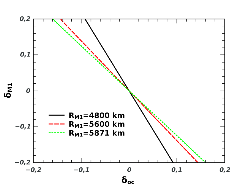
(a)

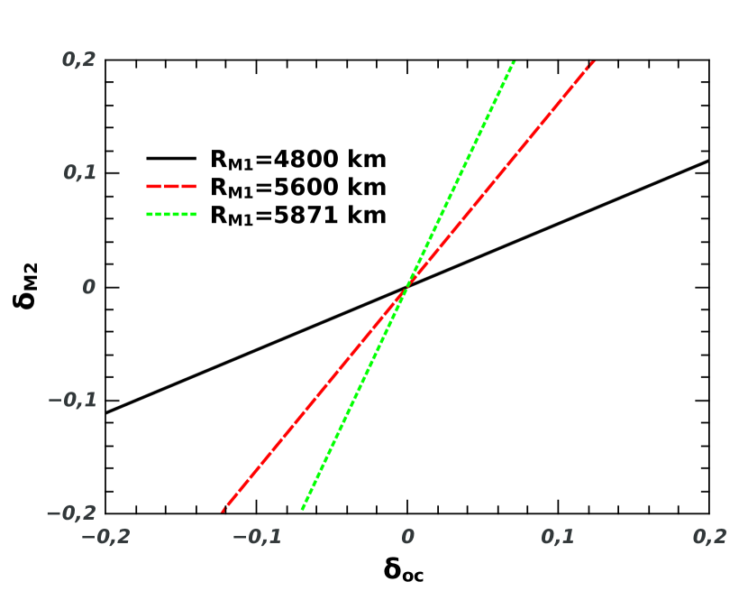
(b)

Figure 2: Relative changes in the densities of the layers (a) $M_{1}$ and (b) $M_{2}$ as a function of the relative change in the density of the outer core, for $R_{M_{1}}$equal to 4800 km, 5600 km, and 5871 km.

Parameter	Normal Ordering	Inverted Ordering
$\Delta m^{2}_{21}$ [$\text{eV}^{2}$]	$7.42\times 10^{-5}$	$7.42\times 10^{-5}$
$\Delta m^{2}_{31}$ [$\text{eV}^{2}$]	$2.533\times 10^{-3}$	$-2.437\times 10^{-3}$
$\sin^{2}{\theta_{12}}$	0.309	0.308
$\sin^{2}{\theta_{13}}$	0.0223	0.0232
$\sin^{2}{\theta_{23}}$	0.561	0.564
$\delta/\pi$	$1.19$	$1.54$

Table 2: Three-neutrino oscillation parameters obtained by averaging the best-fit values of three recent global fits of the current neutrino oscillation data Capozzi:2020 ; Esteban:2020cvm ; deSalas:2020pgw .

3 Atmospheric neutrino oscillations

Neutrino oscillations are a well-verified and widely studied phenomenon that has proven beyond any doubt that neutrinos are mixed massive particles. The current experimental and observational data set can be interpreted in terms of the minimal extension of the Standard Model, where the known flavor states $|{\nu}_{\alpha}\rangle(\alpha=e,\mu,\tau)$ are linear combinations of the states $|{\nu}_{i}\rangle$ with masses $m_{i}\,(i=1,2,3)$: $|{\nu}_{\alpha}\rangle=\sum_{i}U^{*}_{\alpha i}|{\nu}_{i}\rangle.$ The coefficients $U_{\alpha i}$ appear in the leptonic charged current and are elements of a unitary matrix $U$. For for Dirac neutrinos, this matrix can be expressed as $U={\cal O}_{23}\rm\Gamma{\cal O}_{13}{\cal O}_{12}\rm\Gamma^{*}\!,$ with

$${\cal O}_{12}=\left(\begin{array}[]{ccc}c_{12}&s_{12}&0\\ -s_{12}&c_{12}&0\\ 0&0&1\end{array}\right), \ {\cal O}_{13}=\left(\begin{array}[]{ccc}c_{13}&0&s_{13}\\ 0&1&0\\ -s_{13}&0&c_{13}\end{array}\right),$$ (12)

$${\cal O}_{23}=\left(\begin{array}[]{ccc}1&0&0\\ 0&c_{23}&s_{23}\\ 0&-s_{23}&c_{23}\end{array}\right), \!\!\!\Gamma=\left(\begin{array}[]{ccc}1&0&0\\ 0&1&0\\ 0&0&{\rm e}^{i\delta}\end{array}\right),$$ (19)

where $c_{ij}=\cos\theta_{ij}$ and $s_{ij}=\sin\theta_{ij}$. A value of $\delta$ different form 0 or $\pi$ implies CP-violation in the leptonic sector of the theory ​​.

In addition to the mixing angles $\theta_{ij}$ and the CP-violating phase $\delta$, the oscillations between the three active neutrinos are parametrized by two squared-mass differences: $\Delta m^{2}_{21}\equiv m^{2}_{2}-m^{2}_{1}$ and $\Delta m^{2}_{32}\equiv m^{2}_{3}-m^{2}_{1}$. Five of the parameters ($\theta_{12},\theta_{13},\theta_{23},\Delta m^{2}_{21}$, and $|\Delta m^{2}_{31}|$), have been determined with remarkable precision ($\thicksim 1-5\%$) by global fits of the data from solar, atmospheric, reactor and long baseline experiments. The issues still pending are: the sign of $\Delta m^{2}_{31}$, the $\theta_{23}$ octant, and the determination orfthe phase $\delta$. The sign of $\Delta m^{2}_{31}$ characterize the normal ordering (NO), with $m_{3}>m_{1,2}$, and the inverted ordering (IO), with $m_{3}<m_{1,2}$. The 3$\nu$ oscillation parameters shown in Table 2 are the mean of the best-fit values for the allowed ranges at $1\sigma$ of the global analyses performed by three groups Capozzi:2020 ; Esteban:2020cvm ; deSalas:2020pgw .

Neutrinos are produced and detected as flavor eigenstates. Consider a neutrino $\nu_{\alpha}$ produced at time $t_{0}$ that propagates in vacuum. Due to slight mass differences, the phases of the mass eigenstate components of the original flavor state change at different rates and, due to this, the flavor content of the neutrino beam oscillates along the trajectory. When neutrinos propagate in a medium, the coherent forward scattering of neutrinos with electrons is different for $\nu_{e}$ and $\nu_{\mu,\tau}$, resulting in different refraction indexes for the electron neutrino and the other flavors. As a consequence, neutrino oscillations can be significantly modified in matter compared to oscillations in vacuum and new resonance enhancement effects appear. These effects are sensitive to the density and composition of the medium and we will take advantage of this in order to examine the inner parts of our planet by means of the oscillations of atmospheric neutrinos in the Earth. Atmospheric neutrinos have played a very important role in the study and characterization of the phenomena of neutrino oscillations. They are generated around the Earth as decay products in hadronic showers that result from collisions of cosmic rays with nuclei in the upper atmosphere. This provide a continuous source of neutrinos spanning a very wide range of energies and travelled distances before detection. On this work, we concentrate on those with energies in the range of 1-10 GeV and different nadir angles.

Let a neutrino $\nu_{\alpha}$ that enters the solid terrestrial matter at time $t_{0}$. At any time $t>t_{0}$ the state of the system $|\psi(t)\rangle$ can be expressed as $|\psi(t)\rangle=\hat{\mathcal{U}}(t,t_{0})|\psi(t_{0})\rangle$, where $|\psi(t_{0})\rangle=|\nu_{\alpha}\rangle$ and $\hat{\mathcal{U}}(t,t_{0})$ is the evolution operator. The probability of having a neutrino of flavor $\beta$ inside the Earth, at a distance $\ell\simeq t-t_{0}\hskip 0.56917pt(\hslash=c=1)$ from the entry point, is

$$P_{{\nu_{\alpha}}\to{\nu_{\beta}}}(\ell)=|\,{\mathcal{U}}_{\beta\alpha}(\ell)|^{2}\,,$$ (20)

where the probability amplitude ${\mathcal{U}}_{\beta\alpha}(\ell)=\langle\nu_{\beta}|\,\hat{\mathcal{U}}(\ell)|\nu_{\alpha}\rangle$ is an element of the $3\times 3$ unitary matrix $\mathcal{U}(\ell)$ representing the evolution operator in the flavor basis.

Figure 3: Neutrino path through the Earth.

Rather than solving for $\mathcal{U}(\ell)$ directly, it proves to be more convenient to determine the evolution operator in the basis of the mass eigenstates and then transform it to the flavor basis using the relation

$$\mathcal{U}(\ell)=\tilde{U}\tilde{\mathcal{U}}(\ell)\tilde{U}^{\dagger},$$ (21)

where $\tilde{U}={\cal O}_{23}\rm\Gamma{\cal O}_{13}{\cal O}_{12}$.

The matrix $\tilde{\mathcal{U}}(\ell)$ obeys the equation ​

$$i\frac{d}{d\ell}\tilde{\mathcal{U}}(\ell)=\tilde{H}(\ell)\tilde{\mathcal{U}}(\ell),\qquad\tilde{\mathcal{U}}(0)=I,$$ (22)

with

$$\ \tilde{H}(\ell)=H_{\rm 0}+{\mathtt{V}}(\ell){\mathcal{O}}^{\mathtt{T}}Y{\mathcal{O}}\,.$$ (23)

Here, $H_{0}={\rm diag}\{0,\Delta_{21},\Delta_{31}\}$ and $Y={\rm diag}(1,0,0)$ are diagonal matrices and ${\mathcal{O}}^{\mathtt{T}}$ is the transpose of the orthogonal matrix ${\mathcal{O}}={\cal O}_{13}{\cal O}_{12}$. Note that the real and symmetric matrix ${\mathcal{O}}^{\mathtt{T}}Y{\mathcal{O}}$ does not depend on $\theta_{23}$ nor $\delta$. Explicitly,

$${\mathcal{O}}^{\mathtt{T}}Y{\mathcal{O}}=\left(\!\begin{array}[]{ccc}c_{\rm{{\scriptscriptstyle 13}}}^{2}c_{\rm{{\scriptscriptstyle 12}}}^{2}&c_{\rm{{\scriptscriptstyle 12}}}s_{\rm{{\scriptscriptstyle 12}}}c_{\rm{{\scriptscriptstyle 13}}}^{2}&c_{\rm{{\scriptscriptstyle 12}}}c_{\rm{{\scriptscriptstyle 13}}}s_{\rm{{\scriptscriptstyle 13}}}\\ c_{\rm{{\scriptscriptstyle 12}}}s_{\rm{{\scriptscriptstyle 12}}}c_{\rm{{\scriptscriptstyle 13}}}^{2}&s_{\rm{{\scriptscriptstyle 12}}}^{2}c_{\rm{{\scriptscriptstyle 13}}}^{2}&s_{\rm{{\scriptscriptstyle 12}}}c_{\rm{{\scriptscriptstyle 13}}}s_{\rm{{\scriptscriptstyle 13}}}\\ c_{\rm{{\scriptscriptstyle 12}}}s_{\rm{{\scriptscriptstyle 13}}}c_{\rm{{\scriptscriptstyle 13}}}&s_{\rm{{\scriptscriptstyle 12}}}c_{\rm{{\scriptscriptstyle 13}}}s_{\rm{{\scriptscriptstyle 13}}}&s_{\rm{{\scriptscriptstyle 13}}}^{2}\end{array}\!\right)\!.$$ (24)

The first term in Eq. (23) is the Hamiltonian that drives the flavor evolution in vacuum, while the second term accounts for the matter effects. For antineutrinos, the sign of the second term is reversed and the matrix $\rm\Gamma$ is replaced by its complex conjugate.

In normal matter (n, p, e)

$${\mathtt{V}}(\ell)=\sqrt{2}G_{F}n_{e}(\ell)\,,$$ (25)

where $n_{e}(\ell)$ is the electron number density and $G_{F}$ is the Fermi constant. The electron number density depends on both the matter density $\rho(\ell)$ and the chemical and isotopic composition of the medium:

$$n_{e}(\ell)=\dfrac{{\rho}(\ell)}{m_{\rm u}}\dfrac{Z}{A}(\ell)\,,$$ (26)

where $m_{\rm u}=931.494$ MeV is the atomic mass unit and $Z/A=\sum_{\lambda}\digamma_{\!\!\lambda}(Z/A)_{\lambda}.$ The summation runs over all the chemical elements present in the medium and $(Z/A)_{\lambda}$ denotes the ratio between the atomic number $Z_{\lambda}$ and the atomic mass $A_{\lambda}$ of the element that contributes a fraction $\digamma_{\!\!\lambda}$ to the mass at a given position.

The relevant quantities for us are the oscillation probabilities for ${\nu_{\mu}}(\bar{\nu}_{\mu})\to{\nu_{\mu.\tau}}(\bar{\nu}_{\mu,\tau})$ and ${\nu_{e}}(\bar{\nu}_{e})\to{\nu_{\mu,\tau}}(\bar{\nu}_{\mu,\tau})$, which are required to compute the $\mu$-like events produced in a detector by “upward” atmospheric neutrinos after traveling a distance $L=2R_{{}_{\oplus}}\cos\eta$ through the Earth (see Eq. (4)). According to the previous considerations, because of the dependence of these probabilities on the potential ${\mathtt{V}}(\ell)$, atmospheric neutrinos are sensitive to changes in the density and composition of the traversed layers. In what follows, we examine the feasibility of applying such an effect to obtain meaningful information about the deepest part of the Earth. With this in mind, we calculate $\tilde{\mathcal{U}}(L)$ for the Earth modeled as a sphere made up of 55 concentric spherical shells with different (constant) densities, as described in Sec. (2).

The complete evolution operator can be expressed as the product of the evolution operators for the consecutive shells through which the neutrinos pass on their way to the detector:

$$\tilde{\cal U}(L)=\prod_{j=1}^{2j_{m}-1}\tilde{\cal U}_{j}(L_{j})\,,$$ (27)

where $L_{J}$ are the distances in each shell, such that $L=\sum_{j}L_{j}$ and

$$\tilde{\cal U}_{j}(L_{j})=\exp(-i{\tilde{H}}_{j}L_{j})\,.$$ (28)

The effective potential in ${\tilde{H}}_{j}$ takes the fixed value ${\mathtt{V}}_{j}=\sqrt{2}\hskip 0.85355ptG_{F}n^{j}_{e},$ where $n^{j}_{e}$ denotes the constant number density of electrons in shell $j$. Since the Hamiltonians for the different layers do not generally commute between them, the exponential factors in Eq. (27) must be in the prescribed order. Each of these factors can be evaluated by applying the Cayley-Hamilton theorem which allows us to convert the infinity series into a polynomial: $\tilde{\mathcal{U}}_{j}(L_{j})=a^{j}_{0}I+a^{j}_{1}{\tilde{H}}_{\ell}+a^{j}_{2}{\tilde{H}}_{\ell}^{2}\,,$ where the coefficients are functions of the eigenvalues of ${\tilde{H}}_{j}$ (which coincide with those of $H_{j}$) Ohlsson:1999xb ; DOlivo:2020ssf .

Set	$f_{oc}$	$f_{(Z/A)_{oc}}$	$f_{(Z/A)_{M_{1}}}$
I	1	1	1
II	1	1.01	1
III	1.01	1	1
IV	1	1	1.01

Table 3: Different sets of density and composition.

The distances $L_{j}$ are functions of the nadir angle $\eta$. According to Fig. 3, they can be determined as $L_{j}=|\tilde{z}_{j+1}-\tilde{z}_{j}|$, where

$$\tilde{z}_{j}=\begin{cases}z^{+}_{j}\,,&1\leq j\leq j_{m}\,,\\ z^{-}_{2j_{m}+1-j}\,,&j_{m}+1\leq j\leq 2j_{m}\,,\end{cases}$$ (29)

$$z^{\pm}_{j}=R_{{}_{\oplus}}\cos\eta\pm\sqrt{r_{j}^{2}-(R_{{}_{\oplus}}\sin\eta)^{2}}\,.$$ (30)

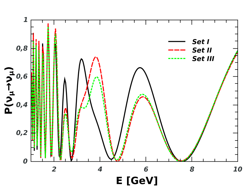
(a) NO and $\eta=20^{\circ}$

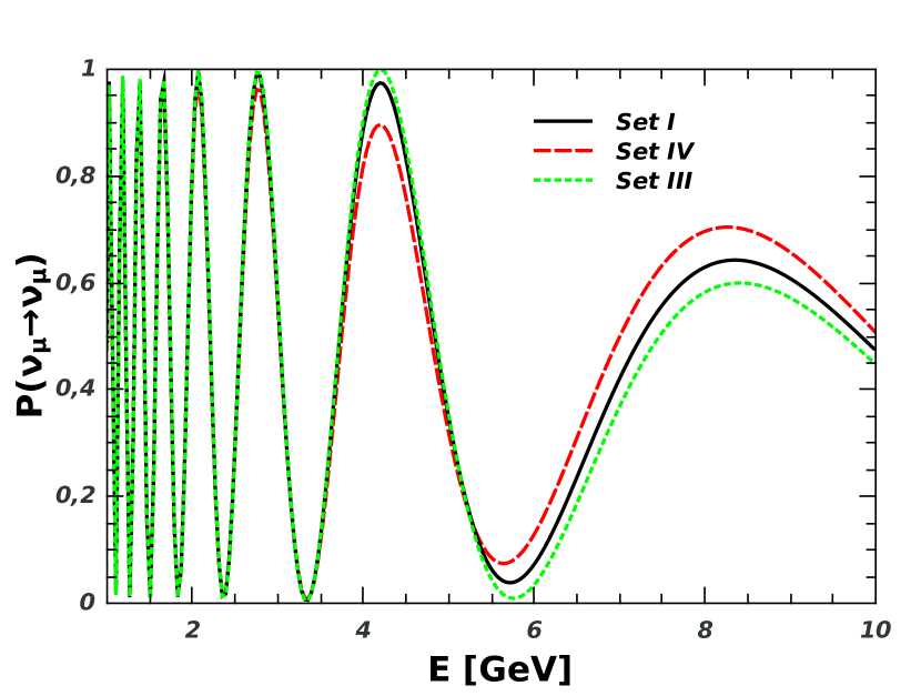
(b) NO and $\eta=50^{\circ}$

Figure 4: Survival probability $P_{{\nu_{\mu}}\to{\nu_{\mu}}}$ as a function of the neutrino energy, for normal ordering (NO) and nadir angle $\eta$ equal to (a) $20^{\circ}$ and (b) $50^{\circ}$​.

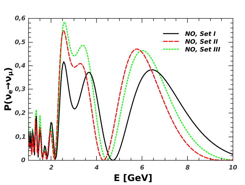
(a) NO and $\eta=20^{\circ}$

(b) IO and $\eta=20^{\circ}$

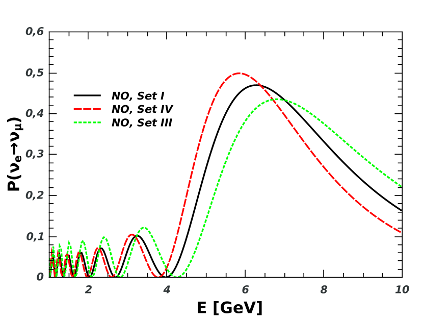
(c) NO and $\eta=50^{\circ}$

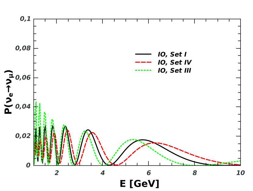
(d) IO and $\eta=50^{\circ}$

Figure 5: Transition probability $P_{{\nu_{e}}\to{\nu_{\mu}}}$ as a function of the neutrino energy, for normal ordering (NO) and inverted ordering (IO) and nadir angle $\eta$ equal to (a,b) $20^{\circ}$ and (c,d) $50^{\circ}$​.

To exemplify the effect that changes in composition and density have on the probabilities of flavor oscillations, in Figs. 4 and 5 we show the probabilities for $\nu_{\mu}\to\nu_{\mu}$ and $\nu_{e}\to\nu_{\mu}$ as functions of the neutrino energy, for two different angles of incidence, both for NO and IO. In the next section, we use these probabilities in the calculation of the $\mu$-like events produced by atmospheric neutrinos arriving at the detector after passing through the internal regions of the Earth.

4 Neutrino events and test of Earth’s composition

Let us consider a generic detector with a mass of water or ice containing a number $n_{{\scriptscriptstyle N}}$ of nucleons as a target. Such a detector, like the planned ORCA, will efficiently detect the Cherenkov radiation emitted along the path of $\mu^{\pm}$ produced by the interactions of $\nu_{\mu}$ and $\bar{\nu}_{\mu}$ with the nucleons in the instrumented volume or near it. In addition, it will be posible to detect showers due to the $e$ or $\tau$ produced by the associated neutrinos Stavropoulos:2021hir ; Kalaczynski:2021ytv ; Bourret:2017tkw .

To generate a data set that simulates the actual observations, with the inevitable statistical fluctuations, we perform a numerical calculation of the events due to neutrinos. Our observable is the number of $\mu$-like events ${\mathcal{N}}_{\mu}$ and in what follows we use it to test different hypothesis about the composition and density of the outer core and the lower part of the mantle. To identify the most sensitive regions, we first do a scan dividing the cone under the detector into a series of angular and energy bins and calculate the number of $\mu$-like events within given angular and energy intervals:

$${\mathcal{N}}_{\mu}=n_{{\scriptscriptstyle N}}T\int_{E_{\text{min}}}^{E_{\text{max}}}\!\differential{E}\int_{\eta_{\text{min}}}^{\eta_{\text{max}}}\differential{\Omega}\left[\sigma^{cc}_{\nu_{\mu}}(E)\left(P_{\nu_{\mu}\rightarrow\nu_{\mu}}{\dfrac{d\Phi}{dE}}^{\!\!\nu_{\mu}}\!+P_{\nu_{e}\rightarrow\nu_{\mu}}{\dfrac{d\Phi}{dE}}^{\!\!\nu_{e}}\right)+\right.$$

$$\left.\sigma^{cc}_{\bar{\nu}_{\mu}}(E)\left(P_{\bar{\nu}_{\mu}\rightarrow\bar{\nu}_{\mu}}{\dfrac{d\Phi}{dE}}^{\!\!\bar{\nu}_{\mu}}\!+P_{\bar{\nu}_{e}\rightarrow\bar{\nu}_{\mu}}{\dfrac{d\Phi}{dE}}^{\!\!\bar{\nu}_{e}}\right)+\right.$$

$$\left.\sigma^{cc}_{\nu_{\tau}}(E)Br_{\tau\rightarrow\mu}\left(P_{\nu_{\mu}\rightarrow\nu_{\tau}}{\dfrac{d\Phi}{dE}}^{\!\!\nu_{\mu}}\!+P_{\nu_{e}\rightarrow\nu_{\tau}}{\dfrac{d\Phi}{dE}}^{\!\!\nu_{e}}\right)+\right.$$

$$\left.\sigma^{cc}_{\bar{\nu}_{\tau}}(E)Br_{\bar{\tau}\rightarrow\bar{\mu}}\left(P_{\bar{\nu}_{\mu}\rightarrow\bar{\nu}_{\tau}}{\dfrac{d\Phi}{dE}}^{\!\!\bar{\nu}_{\mu}}\!+P_{\bar{\nu}_{e}\rightarrow\bar{\nu}_{\tau}}{\dfrac{d\Phi}{dE}}^{\!\!\bar{\nu}_{e}}\right)\right],$$ (31)

where $T$ is the detection time. The fluxes of atmospheric neutrinos and antineutrinos were taken from Ref. Atmnu:1996 , while the charged-current cross sections for the ${\nu}_{\mu}(\bar{\nu}_{\mu})$- nucleon and ${\nu}_{\tau}(\bar{\nu}_{\tau})$-nucleon scatterings, in the considered range of neutrino energies ($1-10$ GeV), are given approximately by Formaggio:2013kya :

$$\sigma^{cc}_{\nu_{\mu}}(E) \simeq 0.75\times 10^{-38}\left({E}/{\rm GeV}\right){\rm cm}^{2}\,,$$ (32)

$$\sigma^{cc}_{\bar{\nu}_{\mu}}(E) \simeq 0.35\times 10^{-38}\left({E}/{\rm GeV}\right){\rm cm}^{2}\,,$$

$$\sigma^{cc}_{\nu_{\tau}}(E) \simeq 0.13\times 10^{-38}\left({E}/{\rm GeV}\right){\rm cm}^{2}\,,$$

$$\sigma^{cc}_{\bar{\nu}_{\tau}}(E) \simeq 0.05\times 10^{-38}\left({E}/{\rm GeV}\right){\rm cm}^{2}\,.$$

In Eq. (4), $Br_{\tau\rightarrow\mu}=Br_{\bar{\tau}\rightarrow\bar{\mu}}\simeq 0.17$ are the branching ratios of the decays $\tau\rightarrow\mu{\bar{\nu}}_{\mu}\nu_{\tau}$ and $\bar{\tau}\rightarrow{\bar{\mu}}{\nu_{\mu}}{\bar{\nu}}_{\tau}$. The dependence of ${\mathcal{N}}_{\mu}$ on the density and composition of the medium is incorporated through the oscillation probabilities, which are calculated from the expressions given in Sec. 3. It is understood that these probabilities are evaluated at $L$. The values of the oscillation parameters are those given in Table 2. To estimate the impact of current uncertainties on the oscillation parameters, in addition to the best fits, we consider their values at the extremes of the 1$\sigma$ ranges Capozzi:2020 ; Esteban:2020cvm ; deSalas:2020pgw . Thus, the muon numbers were also calculated by evaluating the oscillation probabilities at those values of a given parameter and keeping the best fits for the rest. We find that errors in the oscillation parameters introduce only few percent variations in the number of muon events and have little effect on our analysis.

To determine the angular and energy intervals where ${\mathcal{N}}_{\mu}$ is more sensitive to changes in the compositions of either the outer core or the lower mantle we introduce the quantity

$${\Upsilon}(E,\eta)\equiv\absolutevalue{1-\dfrac{\mathcal{N}_{\mu}^{(Z/A)}}{\mathcal{N}_{\mu}^{0}}}\times 100\,,$$ (33)

which gives the percentage difference between the number of events for the standard composition $\mathcal{N}_{\mu}^{0}$ and the number of events for a different composition $\mathcal{N}_{\mu}^{\rm(Z/A)}$. The radii of the layers and the densities of the shells in the layers are those given from the PREM.

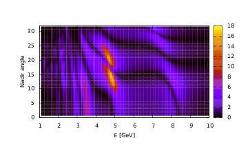
(a) Normal Ordering

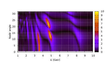
(b) Inverse Ordering

Figure 6: Level surfaces of the function $\Upsilon(E,\eta)$ (Eq. (33)) in the ($E,\eta$) plane, for a $1\%$ change in the composition of the outer core.

Figs. 6 and 7 show the level surfaces of $\Upsilon$ in the ($E,\eta$) plane for a change of $1\%$ in the composition of the outer-core and the composition of the $M_{1}$ region, respectively, for both NO and IO. From the figures, it is apparent that in the case of the outer core the most sensitive regions correspond to energies around 5 GeV and angles compatible with the shadow of the outer core and $M_{1}$. On the other hand, for the lower mantle the angular region has to be increased and the energy shifts to slightly lower values. The deviations in the number of events are considerably more pronounced for NO, mainly because for IO the resonance effects in matter occur for antineutrinos, whose charged cross-section is about two times smaller than that of neutrinos.

To simulate the number of events observed by a km³ detector as ORCA, we follow the same procedure implemented in DOlivo:2020ssf , which we reproduce here for completeness.

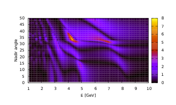
(a) Normal Ordering

(b) Inverse Ordering

Figure 7: Level surfaces of the function $\Upsilon(E,\eta)$ (Eq. (33)) in the ($E,\eta$) plane, for a $1\%$ change in the composition of layer $M_{1}$.

In order to perform the Monte Carlo simulation, based on the previous results, we consider events with $4\,\text{GeV}<E<11\,\text{GeV}$ and $10\degree<\,\eta\,<60\degree$. Both of these intervals are divided into $200$ subintervals. Every pseudo experiment is made up by tossing, in each square bin of the grid, a number of Poisson distributed events with the mean value equal to ${\mathcal{N}}_{\mu}$ as given by Eq. (4). Thus, each of the $n_{exp}$ pseudo experiments consists of 200 $\times$ 200 numbers corresponding to events, one for each bin. This sample of events are then distributed in angle and energy. We call them the true events and suppose that they are distributed according to the probability distribution function (pdf) $f^{\,i_{exp}}_{t}(E,\eta)$, ${i_{exp}}=1,\cdots,n_{exp}$. For this function we take the normalized histograms constructed by means of the Monte Carlo simulation. The fractional number of true events in bin $(i,j)$ for the $i_{exp}$-th experiment is given by the integral of $f^{\,i_{exp}}_{t}(E,\eta)$ over the energy and angle intervals of the bin $(i,j)$.

To obtain a realistic distribution of events we must allow for a limited resolution of the detector, both in energy and angle. The net effect is the redistribution of the true events ("smearing") in the grid bins, which is implemented by folding the true distribution with a resolution function $\mathcal{S}(E_{\mathtt{o}},\eta_{\mathtt{o}}|E,\eta)$. We assume a Gaussian smearing and write

$$\mathcal{S}(E_{\mathtt{o}},\eta_{\mathtt{o}}|E,\eta)=\dfrac{1}{2\pi\Delta\eta(E)\Delta E(E)}\exp\left(-\dfrac{(\eta-\eta_{\mathtt{o}})^{2}}{2\Delta\eta(E)^{2}}\right)\exp\left(-\dfrac{(E-E_{\mathtt{o}})^{2}}{2\Delta E(E)^{2}}\right),$$ (34)

with the detector characterized by the angular and energy resolutions $\Delta\eta(E)=\alpha_{\eta}/\sqrt{E/\text{GeV}}$ and $\Delta E(E)=\alpha_{E}\,E$, respectively. For the values of the parameters $\alpha_{\eta}$ and $\alpha_{E}$ we consider different situations according to the discussion in Ref. Rott:2015kwa . To keep our analysis as simple as possible we assume a detection efficiency of $100\%$. When convoluted with the true events the kernel in Eq. 34 gives us what we call the observed events. That is, $\mathcal{S}(E_{\mathtt{o}},\eta_{\mathtt{o}}|E,\eta)$ represents the conditional pdf for the measured values to be $(E_{\mathtt{o}},\eta_{\mathtt{o}})$ if the true values were $(E,\eta)$. Since the event is observed somewhere, this function is normalized such that

$$\iint\!{\mathcal{S}}(E_{\mathtt{o}},\eta_{\mathtt{o}}|E,\eta)\differential{E}_{\mathtt{o}}\differential{\eta}_{\mathtt{o}}=1\,.$$ (35)

In terms of the resolution function, the number of observed events $\mathcal{O}^{\,i_{exp}}_{m,n}$ in the bin $(m,n)$ for the $i_{exp}$-th experiment is given by

$$\mathcal{O}^{\,i_{exp}}_{m,n}={\mathcal{N}}_{tot}\sum\limits_{i,j}\iint_{\text{bin}\;m,n}\!\differential{E}_{\mathtt{o}}\,\differential{\eta}_{\mathtt{o}}\;\iint_{\text{bin}\;i,j}\!\differential{E}\,\differential{\eta}\;\mathcal{S}(E_{\mathtt{o}},\eta_{\mathtt{o}}|E,\eta)f^{\,i_{exp}}_{t}(E,\eta)\,.$$ (36)

As an illustration, in Fig. 8 and Fig. 9 we show the pdf of the true and observed events as functions of the energy and nadir angle, for NO and IO, respectively, in the case of a standard Earth. The figures were made using the same (large) number of bins for both kind of events, but these numbers generally differ. In what follows, to test how well the hypothesis of different Earth compositions is in agreement with the standard Earth, we take the observed events to be distributed into five angular bins and nine energy bins.

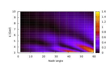
(a)

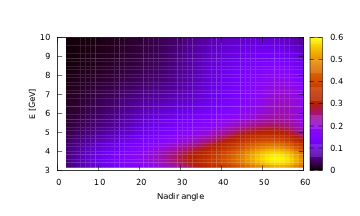
(b)

Figure 8: Probability distribution functions of (a) true events and (b) observed events, as functions of energy and nadir angle, for the standard Earth and normal ordering of neutrino masses. The same number of bins was used to make both figures, but a much small number of bins was used to calculate the observed events.

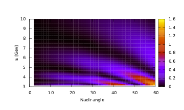
(a)

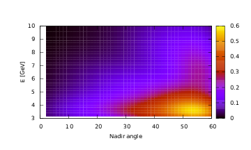
(b)

Figure 9: Probability distribution functions of (a) true events and (b) observed events, as functions of energy and nadir angle, for the standard Earth and inverted ordering of neutrino masses. The same number of bins was used to make both figures, but a much small number of bins was used to calculate the observed events.

From Eq. 36, for each bin $(m,n)$, with $m=1,\cdots,9$ and $n=1,\cdots,5$, we determine the number of events $\mathcal{O}^{\hskip 0.28436pt{\mathtt{s}}i_{exp}}_{\alpha}$ for a standard Earth and $\mathcal{O}^{{\hskip 0.56917pti_{exp}}}_{\alpha}\!({\rm H},\varkappa)$ for an alternative Earth with different composition and density. Here $\alpha=1,\cdots,45$ label the two-dimensional bins ($m,n$). Thus, for each of these bins we have a sample of the observed events and determinate the corresponding mean values

$$\mathcal{\bar{O}}^{\mathtt{s}}_{\alpha} = \frac{1}{n_{exp}}\sum_{i_{exp}}\mathcal{O}^{\hskip 0.28436pt{\mathtt{s}}i_{exp}}_{\alpha}\,,$$

$$\mathcal{\bar{O}}_{\alpha}({\rm H},\varkappa) = \frac{1}{n_{exp}}\sum_{i_{exp}}\mathcal{O}^{{\hskip 0.56917pti_{exp}}}_{\alpha}\!({\rm H},\varkappa)\,.$$ (37)

For Poisson distributed events, in terms of the likelihood function $L$ we construct the negative log-likelihood ratio function as

$$\chi^{2}_{\lambda}=-\ln\left[\frac{L\left(\mathcal{\bar{O}}^{\mathtt{s}}_{\alpha};\mathcal{\bar{O}}_{\alpha}({\rm H},\varkappa)\right)}{L\left(\mathcal{\bar{O}}^{\mathtt{s}}_{\alpha},\mathcal{\bar{O}}^{\mathtt{s}}_{\alpha}\right)}\right]=2\sum_{\alpha}\left[\mathcal{\bar{O}}_{\alpha}({\rm H},\varkappa)-\mathcal{\bar{O}}^{\mathtt{s}}_{\alpha}\ln\left(\frac{\mathcal{\bar{O}}^{\mathtt{s}}_{\alpha}}{\mathcal{\bar{O}}_{\alpha}({\rm H},\varkappa)}\right)\right]\,.$$ (38)

According to Wilks’ theorem wilks1938 the $\chi^{2}_{\lambda}$ distribution can be approximated by the $\chi^{2}$ distribution and, from it, the goodness of the fit can be established. The statistical significance of the $\chi^{2}$ test is given, as usual, by the $\mathbf{p}$-value:

$${\mathbf{p}}=\int_{\chi^{2}}^{\infty}\!f_{\chi}(w,n_{{}_{\!\rm dof}})\differential{w}\,,$$ (39)

where $n_{{}_{\!\rm dof}}$ is the number of degrees of freedom and $f_{\chi}(w,n_{{}_{\!\rm dof}})$ is the chi-square distribution. In our case, $n_{{}_{\!\rm dof}}=9\times 5-2=43$. In this way, we can examine the levels of discrepancy between the standard Earth and different hypothesis about the composition and density of the outer core and the lower mantle. This is done in the next section, where the results and final comments are presented.

5 Results and Final Comments

Our goal is to determine to what extent the presence of light elements, in particular hydrogen, in the outer core and mantle can produce measurable effects due to the modifications it introduces in the flavor transformations of atmospheric neutrinos. We also pay attention to how uncertainties in the densities of the deepest regions of the planet can complicate obtaining compositional information. As discussed in Section 2, we rescale the mantle and outer core densities so that the constraints imposed by the Earth’s total mass and moment of inertia are satisfied. At the same time, we allow for some changes in the compositions of the outer core and/or the lower mantle $M_{1}$.

As the quantities to be fitted, we take the compositions of the outer-core and the lower mantle $M_{1}$ and the densities of the outer core, $M_{1}$ and the rest of the mantle $M_{2}$. To evaluate the effects that changes of two of these quantities have on our observable, we construct regions in several planes: ($\delta_{{\scriptscriptstyle OC}},(Z/A)_{{\scriptscriptstyle OC}}$), ($\delta_{M_{1}},(Z/A)_{M_{1}}$), and ($(Z/A)_{M_{1}},(Z/A)_{{\scriptscriptstyle OC}}$), where the statistical significance, given by the ${\mathbf{p}}$-value, for the discrepancy between the standard and the modified Earth is less than $1\sigma$. In Fig. (10) and (11) we show these regions for the oscillation parameters given in Table 2, for 10 years operation of an 8 Mton detector as ORCA, with resolution parameters $\alpha_{\eta}=0.25$ and $\alpha_{E}=0.2$. As can be seen, the regions for NO are more restricted than for IO. We consider two different values for the radius of the $M_{1}$ layer: 5600 km and 5871 km, which correspond to the lower and upper border of the transition zone between the lower and upper mantle.

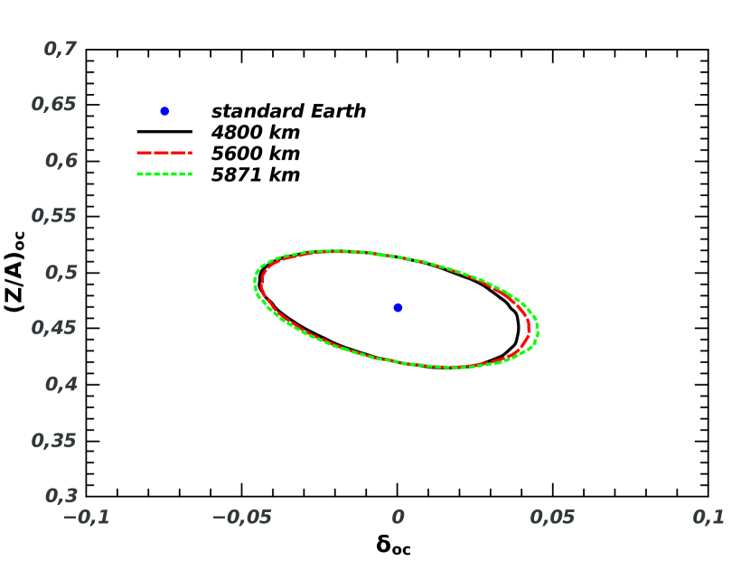
(a) Composition and density of the outer-core.

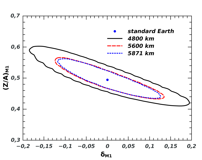
(b) Composition and density of the $M_{1}$ layer.

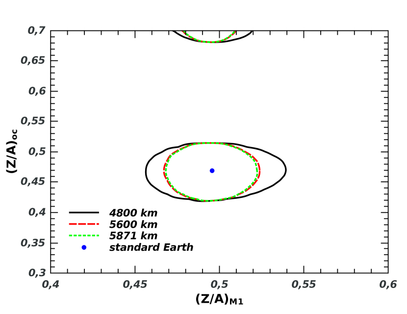
(c) Outer-core and $M_{1}$ compositions.

Figure 10: Expected 1$\sigma$ regions for combined composition and density measures in the outer-core and the $M_{1}$ region, for normal ordering and three values of the $M_{1}$ radii.

In the graphs of composition versus density, non-zero correlations are observed, indicating that increases in composition are compensated by decreases in density, and vice versa, such that the electron density in the shell does not change. This compensation is not complete since, for the Earth’s moment of inertia and mass to remain fixed, variations in density must also occur in other layers traversed by neutrinos and, as a consequence, the allowed regions become closed. The 1$\sigma$ confidence regions for combined measures of Z/A in the outer core and $M_{1}$ agree with those obtained by VanElewyck:2017dga . Suppose that the variation of Z/A in the outer core or mantle is associated only with the abundance of hydrogen, then, as show in Fig.13, $Z/A=(1-\digamma_{\!H})(Z/A)_{0}+\digamma_{\!H}(Z/A)_{H}$, where $(Z/A)_{0}$ is the value with no hydrogen and $\digamma_{\!H}$ is the fractional contribution that hydrogen makes to the total mass of the layer. In this case, the 1$\sigma$ regions are compatible with 5-8 wt% hydrogen in the lower mantle and outer core, respectively, values too high in light of geophysical estimates.

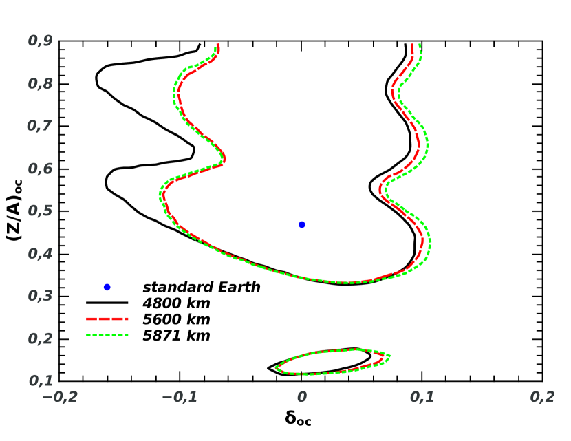
(a) Composition and density of the outer-core.

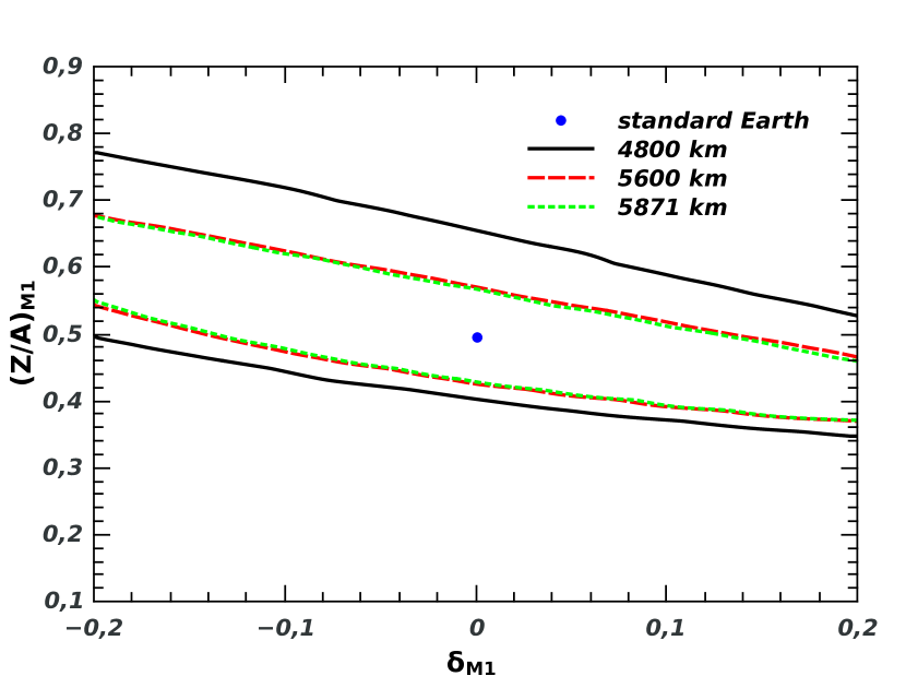
(b) Composition and density of the $M_{1}$ layer.

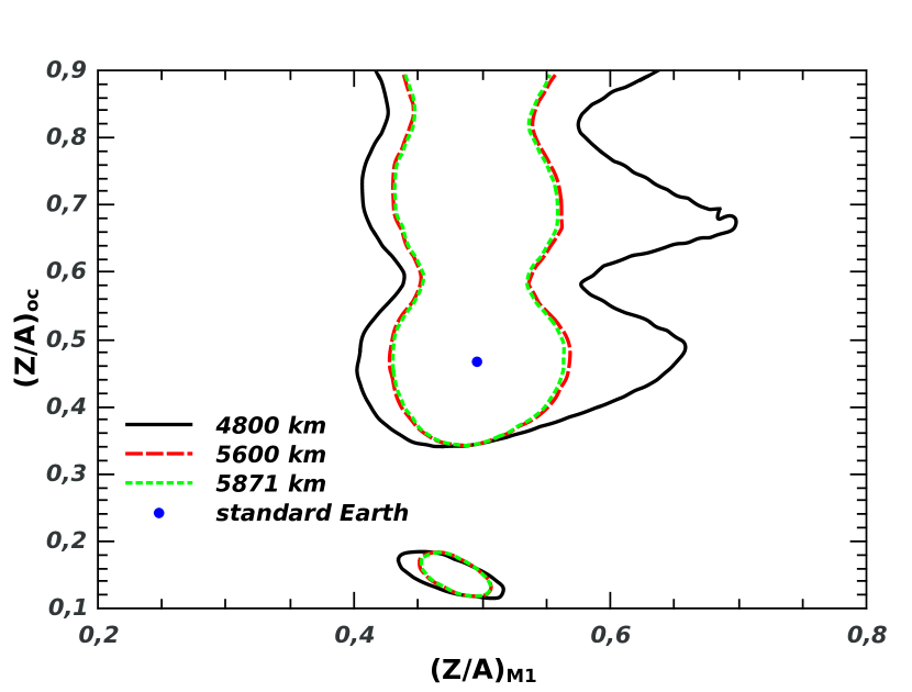
(c) Outer-core and $M_{1}$ composition.

Figure 11: Expected 1$\sigma$ regions for combined composition and density measures in the outer-core and the $M_{1}$ region, for inverted ordering and three values of the $M_{1}$ radii.

As a general rule, for the non fitted parameters we have kept their PREM values. However, for the sake of completeness, we paid some attention to effects from uncertainties in the densities when fitting the compositions. Thus, we have jointly fitted $(Z/A)_{oc},(Z/A)_{M_{1}}$ and $\delta_{oc}$ for the outer core density. (Notice, that the densities of the layers $M_{1}$ and $M_{2}$ vary in order to maintain the values of the Earth’s mass and moment of inertia, as discussed in Section 2). The 1$\sigma$ volume obtained in this way is projected onto the composition-composition plane, giving rise to the shaded area in Fig. 12. The observed negative correlation is caused by the compensation effect in matter neutrino oscillations, with an increase in composition counterbalanced by a decrease in density, and vice versa, to keep the electron number density unchanged. In the case of the composition-density plots (Fig.10(a), Fig.10(b), Fig.11(a), and Fig.11(b)), the uncertainty in the outer core density is incorporated in the lower mantle density, since they are related by Eq. (4).

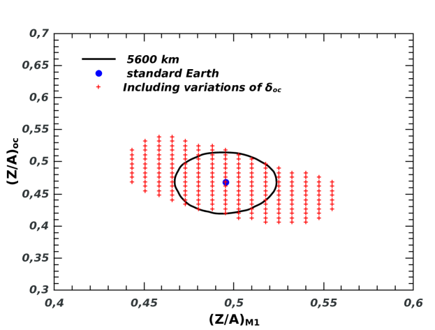
Figure 12: The same region of Fig.10 c, but including the uncertainties in the outer-core densities.

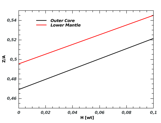
Figure 13: The ratio Z/A as a function of the weight fraction of hydrogen.

As is evident from Figs. 10 and 11, an experiment like ORCA has a limited potential to reveal a non-standard composition and/or density of the Earth. This worsens at 2 and 3$\sigma$ and for the inverted ordering. A question then arises: how much exposure and how much resolution are required to constraint a non-standard composition? As a partial answer, in Fig.14 we shown the1$\sigma$ regions for different exposures (in unity of ten years of ORCA operation) and angular and energy resolutions equal to $\alpha$. We see that with an exposition of thirty years and resolutions of $0.1$ it is possible to constraint the hydrogen content to 1%.

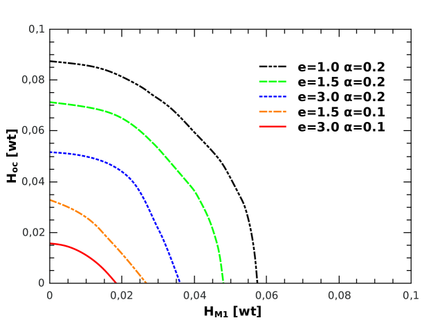
Figure 14: Fraction of hidrogen in the outer-core and the lower mantle for extra exposition $\mathtt{e}$ and resolution $\alpha$.

Finally, we pay special attention to the $D^{\prime\prime}$ region. Since the thickness of this remote interface between the rocky mantle and the iron core is relatively thin, changes in density and composition have little effect on our observable. Fig.15 shows the $1\sigma$ regions for the detector size versus the composition $D^{\prime\prime}$, for a thickness of 200 km and various values of the detector resolution. As can be seen, the allowed regions are not very restrictive for reasonable values of resolution and size of the detector. The ability to constrain the composition is significantly improved in the case of a slightly thicker layer (500 km).

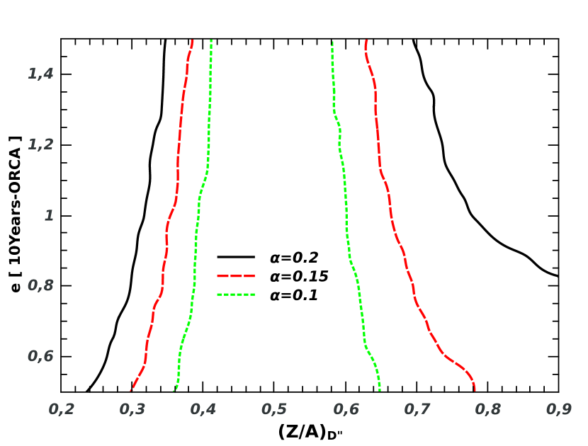
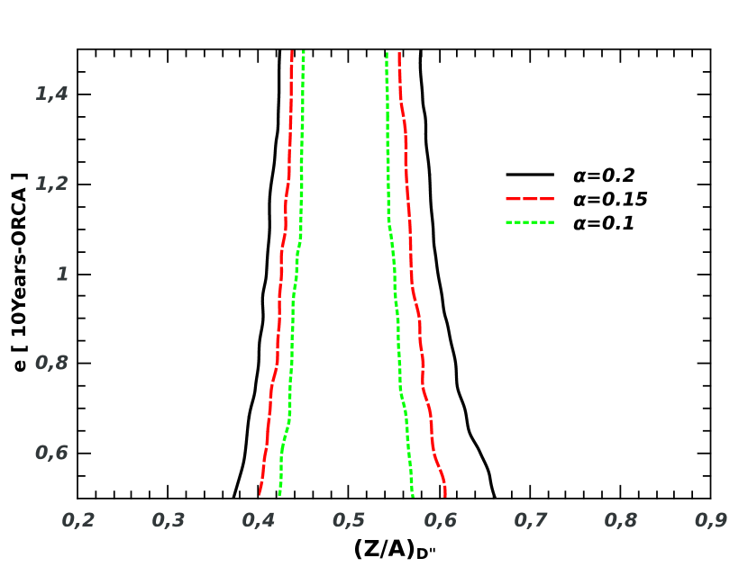
Figure 15: $D^{"}$ composition for different resolutions and size detector. $D^{"}$ thickness $500$ km.

In summary, we have studied the possibility of conducting an oscillation tomography of the Earth based on the matter effects on the flavor oscillations of atmospheric neutrinos propagating through the depths of the planet. Using the $\mu$-like events in a generic large Cherenkov detector as physical observables and making a Monte Carlo simulation of the energy and azimuthal angle distribution of these event, we tested possible variants with respect to a reference geophysical model with the densities as given by PREM and different composition in the outer-core and lower mantle. Unlike previous studies, the procedure we followed in this work allowed us to simultaneously vary the composition and density. When one of these quantities was fixed in the value of the reference geophysical model, our results, shown in Figs. 10, are compatible with those obtained by others authors in an uncorrelated way VanElewyck:2017dga ; Borriello:2009ad . As shown, the study of questions of the type examined here would benefit greatly from the application of phenomena normally studied in the realm of particle physics and the advent of new and improved neutrino telescopes, such as KM3NeT, ORCA, PINGO and HyperK Adrian-Martinez:2016fdl ; Fermani:2019vac ; Hyper-Kamiokande:2018ofw ; Aarsten:2017 .

- (1) E. Tarbuck, F. Lutgens, D. Tasa, Earth Science (Pearson Prentice Hall, 2009)
- (2) C. Fowler, The Solid Earth: An Introduction to Global Geophysics (2 ed.) (Cambridge University Pres, 2005)
- (3) T. Lay, T. Wallace, Modern Global Seismology, International Geophysics Series, vol. 58, 1st edn. (Academic Press, San Diego, 1995)
- (4) K. Aki, P.G. Richards, Quantitative Seismology, 2nd Ed. (University Science Books, 2002)
- (5) G.R. Helffrich, B.J. Wood, Nature 412(6846), 501 (2001). DOI 10.1038/35087500. URL https://doi.org/10.1038/35087500
- (6) D. Loper, L. Thorne, Journal of Geophysical Research 100(B4), 6397 (1995)
- (7) T. Lay, Q. Williams, E. Garnero, Nature 392, 461 (1998)
- (8) M. Murakami, K. Hirose, K. Kawamura, N. Sata, Y. Ohishi, Science 304(5672), 855 (2004). DOI 10.1126/science.1095932. URL https://doi.org/10.1126%2Fscience.1095932
- (9) K. Hirose, B. Wood, L. Vočadlo, Nature Reviews Earth & Environment 2(9), 645 (2021). DOI 10.1038/s43017-021-00203-6. URL https://doi.org/10.1038/s43017-021-00203-6
- (10) F. Birch, Journal of Geophysical Research 57, 4377 (1964)
- (11) J.P. Poirier, Physics of the Earth and Planetary Interiors 85(3), 319 (1994). DOI https://doi.org/10.1016/0031-9201(94)90120-1. URL https://www.sciencedirect.com/science/article/pii/0031920194901201
- (12) K. Litasov, A. Shatskiy, Russian Geology and Geophysics 57, 22 (2016). DOI 10.1016/j.rgg.2016.01.003
- (13) J. Wookey, D.P. Dobson, Philosophical Transactions of the Royal Society A: Mathematical, Physical and Engineering Sciences 366(1885), 4543 (2008). DOI 10.1098/rsta.2008.0184. URL https://doi.org/10.1098%2Frsta.2008.0184
- (14) J.R. Lister, B.A. Buffett, Physics of the Earth and Planetary Interiors 91(1), 17 (1995). DOI https://doi.org/10.1016/0031-9201(95)03042-U. URL https://www.sciencedirect.com/science/article/pii/003192019503042U. Study of the Earth’s Deep Interior
- (15) P.H. Roberts, E.M. King, Reports on Progress in Physics 76(9), 096801 (2013). DOI 10.1088/0034-4885/76/9/096801. URL https://doi.org/10.1088/0034-4885/76/9/096801
- (16) J. Brodholt, J. Badro, Geophysical Research Letters 44(16), 8303 (2017). DOI 10.1002/2017gl074261. URL https://doi.org/10.1002%2F2017gl074261
- (17) B.A. Bolt, Quarterly Journal of the Royal Astronomical Society 32(4), 367 (1991)
- (18) R.J. Geller, T. Hara, Nuclear Instruments and Methods in Physics Research Section A: Accelerators, Spectrometers, Detectors and Associated Equipment 503(1-2), 187 (2003). DOI 10.1016/s0168-9002(03)00670-3. URL https://doi.org/10.1016%2Fs0168-9002%2803%2900670-3
- (19) G. Masters, D. Gubbins, Physics of the Earth and Planetary Interiors 140, 159 (2003). DOI 10.1016/j.pepi.2003.07.008
- (20) W. McDonough, S. s. Sun, Chemical Geology 120(3), 223 (1995). DOI https://doi.org/10.1016/0009-2541(94)00140-4. URL https://www.sciencedirect.com/science/article/pii/0009254194001404. Chemical Evolution of the Mantle
- (21) C.J. Allègre, J.P. Poirier, E. Humler, A.W. Hofmann, Earth and Planetary Science Letters 134(3-4), 515 (1995). DOI 10.1016/0012-821x(95)00123-t. URL https://doi.org/10.1016%2F0012-821x%2895%2900123-t
- (22) Y. Zhang, T. Sekine, H. He, Y. Yu, F. Liu, M. Zhang, Scientific Reports 6(1) (2016). DOI 10.1038/srep22473. URL https://doi.org/10.1038%2Fsrep22473
- (23) D. Alderton, S.A. elias (eds.), Encyclopedia of Geology, second edition edn. 150–163 (Academic Press, 2021)
- (24) M.M. Hirschmann, Annual Review of Earth and Planetary Sciences 34(1), 629 (2006). DOI 10.1146/annurev.earth.34.031405.125211. URL https://doi.org/10.1146/annurev.earth.34.031405.125211
- (25) A.H. Peslier, M. Schönbächler, H. Busemann, S.I. Karato, Space Science Reviews 212(1-2), 743 (2017). DOI 10.1007/s11214-017-0387-z. URL https://doi.org/10.1007%2Fs11214-017-0387-z
- (26) E. Ohtani, National Science Review 7(1), 224 (2019). DOI 10.1093/nsr/nwz071. URL https://doi.org/10.1093%2Fnsr%2Fnwz071
- (27) R. Bodnar, T. Azbej, S. Becker, C. Cannatelli, A. Fall, M. Severs, Special Paper of the Geological Society of America 500, 431 (2013). DOI 10.1130/2013.2500(13)
- (28) E.J. Garnero, A.K. McNamara, S.H. Shim, Nature Geoscience 9(7), 481 (2016). DOI 10.1038/ngeo2733. URL https://doi.org/10.1038%2Fngeo2733
- (29) J.P. Townsend, J. Tsuchiya, C.R. Bina, S.D. Jacobsen, Earth and Planetary Science Letters 454, 20 (2016). DOI 10.1016/j.epsl.2016.08.009. URL https://doi.org/10.1016%2Fj.epsl.2016.08.009
- (30) D.G. Pearson, F.E. Brenker, F. Nestola, J. McNeill, L. Nasdala, M.T. Hutchison, S. Matveev, K. Mather, G. Silversmit, S. Schmitz, B. Vekemans, L. Vincze, Nature 507(7491), 221 (2014). DOI 10.1038/nature13080. URL https://doi.org/10.1038%2Fnature13080
- (31) O. Tschauner, S. Huang, E. Greenberg, V. Prakapenka, C. Ma, G. Rossman, A. Shen, D. Zhang, M. Newville, A. Lanzirotti, et al., Science 359(6380), 1136 (2018)
- (32) S. ichiro Karato, Earth and Planetary Science Letters 301(3), 413 (2011). DOI https://doi.org/10.1016/j.epsl.2010.11.038. URL https://www.sciencedirect.com/science/article/pii/S0012821X10007454
- (33) S.i. Karato, B. Karki, J. Park, Progress in Earth and Planetary Science 7(1), 76 (2020). DOI 10.1186/s40645-020-00379-3. URL https://doi.org/10.1186/s40645-020-00379-3
- (34) H. Fei, D. Yamazaki, M. Sakurai, N. Miyajima, H. Ohfuji, T. Katsura, T. Yamamoto, Science Advances 3(6) (2017). DOI 10.1126/sciadv.1603024. URL https://doi.org/10.1126%2Fsciadv.1603024
- (35) F.D. Munch, A.V. Grayver, M. Guzavina, A.V. Kuvshinov, A. Khan, Geophysical Research Letters 47(10), e2020GL087222 (2020)
- (36) W. Winter, Earth Moon Planets 99, 285 (2006). DOI 10.1007/s11038-006-9101-y
- (37) L. Volkova, G. Zatsepin, Izv. Akad. Nauk Ser. Fiz 38N5, 1060 (1974)
- (38) T.L. Wilson, Nature 309, 38 (1984). DOI 10.1038/309038a0
- (39) J.P. Ralston, P. Jain, G.M. Frichter, in 26th International Cosmic Ray Conference, vol. 2 (1999), vol. 2, p. 504
- (40) P. Jain, J.P. Ralston, G.M. Frichter, Astropart. Phys 12, 193 (1999). DOI 10.1016/S0927-6505(99)00088-2
- (41) M. Gonzalez-Garcia, F. Halzen, M. Maltoni, H.K. Tanaka, Phys. Rev. Lett 100, 061802 (2008). DOI 10.1103/PhysRevLett.100.061802
- (42) M.M. Reynoso, O.A. Sampayo, Astropart. Phys 21, 315 (2004). DOI 10.1016/j.astropartphys.2004.01.003
- (43) I. Romero, O.A. Sampayo, Eur. Phys. J. C 71, 1696 (2011). DOI 10.1140/epjc/s10052-011-1696-0
- (44) A. Donini, S. Palomares-Ruiz, J. Salvado, Nature Phys. 15(1), 37 (2019). DOI 10.1038/s41567-018-0319-1
- (45) L. Wolfenstein, Phys. Rev. D 17, 2369 (1978). DOI 10.1103/PhysRevD.17.2369
- (46) V.D. Barger, K. Whisnant, S. Pakvasa, R. Phillips, Phys. Rev. D 22, 2718 (1980). DOI 10.1103/PhysRevD.22.2718
- (47) S. Mikheyev, A. Smirnov, Sov. J. Nucl. Phys. 42, 913 (1985)
- (48) A. Nicolaidis, Phys. Lett. B 200, 553 (1988). DOI 10.1016/0370-2693(88)90170-0
- (49) A. Nicolaidis, M. Jannane, A. Tarantola, J. Geophys. Res. 96(B13), 21811 (1991). DOI 10.1029/91JB01835
- (50) E. Borriello, G. Mangano, A. Marotta, G. Miele, P. Migliozzi, C. Moura, S. Pastor, O. Pisanti, P.E. Strolin, JCAP 06, 030 (2009). DOI 10.1088/1475-7516/2009/06/030
- (51) W. Winter, Nucl. Phys. B 908, 250 (2016). DOI 10.1016/j.nuclphysb.2016.03.033
- (52) C. Rott, A. Taketa, D. Bose, Sci. Rep 5, 15225 (2015). DOI 10.1038/srep15225
- (53) S. Bourret, J.A. Coelho, V. Van Elewyck, PoS ICRC2017, 1020 (2018). DOI 10.22323/1.301.1020
- (54) S. Bourret, J.a.A.B. Coelho, V. Van Elewyck, J. Phys. Conf. Ser. 888(1), 012114 (2017). DOI 10.1088/1742-6596/888/1/012114
- (55) J.C. D’Olivo, J.A. Herrera Lara, I. Romero, O.A. Sampayo, G. Zapata, Eur. Phys. J. C 80(10), 1001 (2020). DOI 10.1140/epjc/s10052-020-08585-5
- (56) K.J. Kelly, P.A.N. Machado, I. Martinez-Soler, Y.F. Perez-Gonzalez, FERMILAB-PUB-21-459-T, NUHEP-TH/21-15, arXiv/2110.00003 (2021)
- (57) P.B. Denton, R. Pestes, Phys. Rev. D 104(11), 113007 (2021). DOI 10.1103/PhysRevD.104.113007
- (58) A.K. Upadhyay, A. Kumar, S.K. Agarwalla, A. Dighe, IP/BBSR/2021-12, TIFR/TH/21-22, arXiv/2112.14201 (2021)
- (59) A.M. Dziewonski, D.L. Anderson, Physics of the earth and planetary interiors 25(4), 297 (1981)
- (60) B.L.N. Kennett, E.R. Engdahl, R. Buland, Geophysical Journal International 122(1), 108 (1995). DOI 10.1111/j.1365-246X.1995.tb03540.x. URL https://doi.org/10.1111/j.1365-246X.1995.tb03540.x
- (61) J. Williams, The Astronomical Journal 108, 711 (1994). DOI 10.1086/117108
- (62) F. Capozzi, E. Di Valentino, E. Lisi, A. Marrone, A. Melchiorri, A. Palazzo, Phys. Rev. D 101(11), 116013 (2020). DOI 10.1103/PhysRevD.101.116013. URL https://link.aps.org/doi/10.1103/PhysRevD.101.116013
- (63) I. Esteban, M.C. Gonzalez-Garcia, M. Maltoni, T. Schwetz, A. Zhou, JHEP 09, 178 (2020). DOI 10.1007/JHEP09(2020)178
- (64) P.F. de Salas, D.V. Forero, S. Gariazzo, P. Martínez-Miravé, O. Mena, C.A. Ternes, M. Tórtola, J.W.F. Valle, JHEP 02, 071 (2021). DOI 10.1007/JHEP02(2021)071
- (65) S.M. Bilenky, J. Hosek, S. Petcov, Phys. Lett. B 94, 495 (1980). DOI 10.1016/0370-2693(80)90927-2
- (66) T. Ohlsson, H. Snellman, J. Math. Phys. 41, 2768 (2000). DOI 10.1063/1.533270. [Erratum: J.Math.Phys. 42, 2345 (2001)]
- (67) D. Stavropoulos, V. Pestel, Z. Aly, E. Tzamariudaki, C. Markou, PoS ICRC2021, 1125 (2021). DOI 10.22323/1.395.1125
- (68) P. Kalaczyński, PoS ICHEP2020, 149 (2021). DOI 10.22323/1.390.0149
- (69) V. Agrawal, T. Gaisser, P. Lipari, T. Stanev, Phys. Rev. D 53, 1314 (1996). DOI 10.1103/PhysRevD.53.1314
- (70) J. Formaggio, G. Zeller, Rev. Mod. Phys. 84, 1307 (2012). DOI 10.1103/RevModPhys.84.1307
- (71) S.S. Wilks, Ann. Math. Statist. 9(1), 60 (1938). DOI 10.1214/aoms/1177732360. URL https://doi.org/10.1214/aoms/1177732360
- (72) S. Adrian-Martinez, et al., J. Phys. G43(8), 084001 (2016). DOI 10.1088/0954-3899/43/8/084001
- (73) P. Fermani, I. Di Palma, EPJ Web Conf 209, 01006 (2019). DOI 10.1051/epjconf/201920901006
- (74) K. Abe, et al., arxiv/1805.04163 (2018)
- (75) M. Aartsen, et al., Journal of Physics G 44, 054006 (2017). DOI 10.1088/1361-6471/44/5/054006