Path integral molecular dynamics for anyons, bosons and fermions

Abstract

In this article we develop a general method to numerically calculate physical properties for a system of anyons with path integral molecular dynamics. We provide a unified method to calculate the thermodynamics of identical bosons, fermions and anyons. Our method is tested and applied to systems of anyons, bosons and fermions in a two-dimensional harmonic trap. We also consider a method to calculate the energy for fermions as an application of the path integral molecular dynamics to simulate the anyon model.

Keywords: anyons; bosons; fermions; path integral; molecular dynamics

I introduction

Quantum many-body systems are fascinating and reveal much of the interesting phenomenon of nature. In particular, systems consisting of identical particles are of great interests since quantum mechanics dictates that fundamental exchange symmetries be present in such systems. Insightful effects such as Berezinskii-Kosterlitz-Thouless transition Kosterlitz ; Hadzibabic are found resulting from the exchange symmetry between identical particles. Traditionally, people have considered only two kinds of fundamental exchange symmetry in a system of identical particles, with the wave function either be completely symmetric or anti-symmetric, corresponding to bosons and fermions respectively. However, when studying quantum many-body systems in two dimensions, researchers have found that other kinds of exchange symmetry are possible Leinaas . This leads to the discovery of anyons Leinaas ; FluxW ; a-wilczek ; Wilczek ; khare . Anyons manifest novel phenomenon such as fractional quantum Hall effects Tsui and their existences in two dimensional systems are shown by recent experiments Bar ; Nak ; Nak2 .

Aside from experimental study of many-body quantum systems, numerical simulations of such systems are also desirable. There are two main ways to perform the simulations based on path integral formalism feynman ; kleinert : path integral Monte Carlo CeperRMP ; boninsegni1 ; boninsegni2 ; Dornheim and path integral molecular dynamics (PIMD) chandler ; Parrinello ; Tuckerman . Path integral Monte Carlo has been applied successfully to large bosonic systems boninsegni1 ; boninsegni2 , by sampling directly the partition function corresponding to the system under study. However, PIMD has found few applications in the field of identical particles until recently, when an efficient polynomial algorithm Hirshberg to perform PIMD has been developed, enabling applications of PIMD to large bosonic system Hirshberg ; Xiong ; XiongSpinor and fermionic system HirshbergFermi ; Xiong1 . Both of these approaches suffer from severe efficiency issues when applied to identical fermions, due to the so-called fermion sign problem ceperley ; loh ; troyer ; lyubartsev ; vozn ; Yao1 ; Yao2 ; Yao3 .

In this paper we extend PIMD to perform numercial simulations for a system of identical anyons. In particular, we calculate the energies and densities for anyons and study their dependences on the statistical properties for the anyons. Our work provided a unified method to calculate various properties of anyons, bosons and fermions. The paper is organized as follows: In Sec. II, we start by reviewing path integral formulations for anyons. We then present PIMD and show how to extend the technique to perform simulations for a system of identical anyons. In Sec. III, we present our simulation results for the energies and densities for anyons and study their dependences on the statistical properties of the anyons. In Sec. IV, by taking advantage of the extra freedom in choosing the statistical properties for anyons, we suggest a way to calculate the energy of a few fermions by an extrapolation with a simple function based on reasonable physical considerations. In Sec. V, we give a concise summary and discussion of our work.

II theory

II.1 Path integral for anyons, bosons and fermions

In this paper, we will use "boson" gauge to consider the anyons in a general way Myrheim . The derivation from Bose-Einstein statistics in this bosonic gauge is due to a "statistics" field, which is a vector potential based on the flux-tube model for anyons by Wilczek FluxW . The Bose statistics may change continuously into Fermi statistics when the statistics angle $\theta$ changes from boson value $0$ to fermion value $\pi$. The fractional statistics is the situation of $0<\theta<\pi$. In this case, it is anticipated that there would be a general numerical method which can be applied to both bosons and fermions in a unified way.

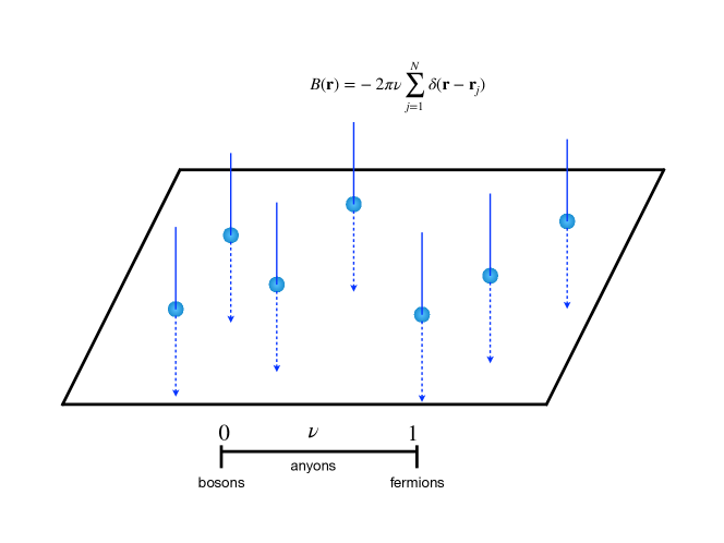
Figure 1: The flux-tube model for anyons.

In the flux-tuble model for anyons FluxW , the anyons turn out to be point particles having a fictitious magnetic flux. In this case, the flux is located exactly at the position of the $j$th particle, and the fictitious magnetic field for this particle is

$$B(\mathbf{r})=-2\pi\nu\delta(\mathbf{r}-\mathbf{r}_{j}).$$ (1)

Here $\nu$ is a parameter for the statistical properties of the anyon. $\nu=0$ for bosons and $\nu=1$ for fermions. The statistics angle $\theta=\nu\pi$. For $N$ anyons, the total magnetic field is

$$B(\mathbf{r})=-2\pi\nu\sum_{j=1}^{N}\delta(\mathbf{r}-\mathbf{r}_{j}).$$ (2)

From the relation between $B$ and the vector potential $\mathbf{A}$

$$B=\partial_{x}A_{y}-\partial_{y}A_{x},$$ (3)

we have the following vector potential at $\mathbf{r}$ generated by the $j$th particle,

$$A_{x}^{j}(\mathbf{r})=\nu\frac{y-y_{j}}{(x-x_{j})^{2}+(y-y_{j})^{2}},$$

$$A_{y}^{j}(\mathbf{r})=-\nu\frac{x-x_{j}}{(x-x_{j})^{2}+(y-y_{j})^{2}}.$$ (4)

The N-particle Hamiltonian is

$$\hat{H}_{N}=\frac{1}{2m}\sum_{j=1}^{N}\left(\hat{\mathbf{p}}_{j}-\hbar{\mathbf{a}}_{j}\right)^{2}+V.$$ (5)

Here $\hat{\mathbf{p}}_{j}$ is the canonical momentum of the $j$th particle. $V$ is the interaction potential including both the external potential and interaction potential between anyons. The statistical interaction is due to the vector potential ${\mathbf{a}}_{j}$ for the $j$th particle. Because this vector potential is due to all other particles, we have

$$a_{jx}(\mathbf{r}_{j})=\nu\sum_{k\neq j}\frac{y_{j}-y_{k}}{(x_{j}-x_{k})^{2}+(y_{j}-y_{k})^{2}},$$

$$a_{jy}(\mathbf{r}_{j})=-\nu\sum_{k\neq j}\frac{x_{j}-x_{k}}{(x_{j}-x_{k})^{2}+(y_{j}-y_{k})^{2}}.$$ (6)

II.2 The path integral for anyons

The partition function for $N$ anyons is

$$Z_{A}(\beta)=Tre^{-\beta\hat{H}_{N}}.$$ (7)

Here $\beta=1/k_{B}T$ with $k_{B}$ the Boltzmann constant and $T$ the temperature of the system. Because we use the bosonic gauge to consider the anyons, we have

$$Z_{A}(\beta)=\frac{1}{N!}\sum_{p\in S_{N}}\int d\mathbf{r}_{1}\cdots d\mathbf{r}_{N}\left<p\{\mathbf{r}_{1},\cdots,\mathbf{r}_{N}\}\right|e^{-\beta\hat{H}_{N}}\left|\mathbf{r}_{1},\cdots,\mathbf{r}_{N}\right>.$$ (8)

Here $p$ denotes $N!$ permutation of $S_{N}$ permutation group. The integral is about the usual $\mathbf{R}^{dN}$ space.

We divide $\beta$ into $P$ intervals (let us denote the interval length by $\Delta\beta=\beta/P$) and expand each of the evolution operators into products of the form

$$e^{-\beta\hat{H}}=e^{-\Delta\beta\hat{H}}\cdots e^{-\Delta\beta\hat{H}}.$$ (9)

In the limit of $P\rightarrow\infty$, we have

$$Z_{A}(\beta)=\frac{1}{N!}\sum_{p\in S_{N}}\int_{\mathcal{C}(p)}\mathcal{D}[\mathbf{r}_{1}(\tau),\cdots,\mathbf{r}_{N}(\tau)]e^{-\frac{S}{\hbar}-i\theta Q}.$$ (10)

Here

$$S=\int_{0}^{\hbar\beta}d\tau\left(\frac{m}{2}\sum_{j=1}^{N}\left|\frac{d\mathbf{r}_{j}}{d\tau}\right|^{2}+V(\mathbf{r}_{1}\cdots\mathbf{r}_{N})\right),$$ (11)

and

$$-\theta Q=-\pi\nu Q=\sum_{j=1}^{N}\int d\mathbf{r}_{j}\cdot\mathbf{a}_{j}(\mathbf{r}_{j}).$$ (12)

This equation stands for the sum of a series of line integrals. To evaluate such line integrals some parametrization of the curve must be chosen. Of course the variable $\tau$ provides a natural parametrization and this was used in our numerical calculation, but generally any parametrization works and leads to the same result for the integral. We chose to write the line integral in the general form in Eq. (12), whereas the discrete form based on $\tau$ parametrization will be presented in Eq. (15). In the above equation for $Z_{A}(\beta)$, the domain of integration $\mathcal{C}(p)$ represents $\{\mathbf{r}_{1}(\hbar\beta),\cdots\mathbf{r}_{N}(\hbar\beta)\}=p\{\mathbf{r}_{1}(0),\cdots,\mathbf{r}_{N}(0)\}$.

In our numerical calculations, $P$ is always finite. In this case, the approximate $Z_{A}(\beta)$ can be written as

$$Z_{A}(\beta)=\left(\frac{mP}{2\pi\hbar^{2}\beta}\right)^{PdN/2}\int e^{-\beta(V_{B}^{(N)}+\frac{1}{P}U)}e^{-i\theta\Phi}d\mathbf{R}_{1}...d\mathbf{R}_{N},$$ (13)

where $\mathbf{R}_{i}$ represents the collection of ring polymer coordinates $(\mathbf{r}_{i}^{1},...,\mathbf{r}_{i}^{P})$ corresponding to the $i$th particle. The system considered has $d$ spatial dimensions. For anyons considered in this work, $d=2$. $V_{B}^{(N)}$ considers exchange effects by describing all the possible ring polymer configurations. $U$ is the interaction between different particles, which is given by

$$U=\sum_{l=1}^{P}V(\mathbf{r}_{1}^{l},...,\mathbf{r}_{N}^{l}).$$ (14)

In addition,

$$-\theta\Phi(\mathbf{R}_{1},...,\mathbf{R}_{N})=\sum_{j=1}^{N}\sum_{l=1}^{P-1}(\mathbf{r}_{j}^{l+1}-\mathbf{r}_{j}^{l})\cdot\mathbf{a}_{j}(\mathbf{r}_{1}^{l},...,\mathbf{r}_{N}^{l}),$$ (15)

where $\mathbf{a}_{j}(\mathbf{r}_{1}^{l},...,\mathbf{r}_{N}^{l})$ is given by

$$a_{jx}(\mathbf{r}_{1}^{l},...,\mathbf{r}_{N}^{l})=\nu\sum_{k\neq j}\frac{r_{jy}^{l}-r_{ky}^{l}}{(r_{jx}^{l}-r_{kx}^{l})^{2}+(r_{jy}^{l}-r_{ky}^{l})^{2}},$$

$$a_{jy}(\mathbf{r}_{1}^{l},...,\mathbf{r}_{N}^{l})=-\nu\sum_{k\neq j}\frac{r_{jx}^{l}-r_{kx}^{l}}{(r_{jx}^{l}-r_{kx}^{l})^{2}+(r_{jy}^{l}-r_{ky}^{l})^{2}}.$$ (16)

The expression of $V_{B}^{(N)}$ is the key to consider the exchange effects of identical bosons, which will be introduced in due course.

II.3 Path integral molecular dynamics

To carry out the numerical calculations, we should give the expression of $V_{B}^{(N)}$. Fortunately, in Ref. Hirshberg , it is given for path integral molecular dynamics of bosons. In our bosonic gauge for anyons, because the factor $\theta Q$ is symmetric about the exchange of $\mathbf{r}_{i}$ and $\mathbf{r}_{j}$, the recursion formula of $V_{B}^{(N)}$ can be used without any change.

The recursion formula is

$$e^{-\beta V_{B}^{(\alpha)}}=\frac{1}{\alpha}\sum_{k=1}^{\alpha}e^{-\beta(E_{\alpha}^{(k)}+V_{B}^{(\alpha-k)})},$$ (17)

where $V_{B}^{(0)}=0$ and $E_{\alpha}^{(k)}$ is given by

$$E_{\alpha}^{(k)}(\mathbf{R}_{\alpha-k+1},...,\mathbf{R}_{\alpha})=\frac{1}{2}m\omega_{P}^{2}\sum_{l=\alpha-k+1}^{\alpha}\sum_{j=1}^{P}(\mathbf{r}_{l}^{j+1}-\mathbf{r}_{l}^{j})^{2},$$ (18)

where $\mathbf{r}_{l}^{P+1}=\mathbf{r}_{\alpha-k+1}^{1}$ if $l=\alpha$ and $\mathbf{r}_{l}^{P+1}=\mathbf{r}_{l+1}^{1}$ otherwise. $E_{\alpha}^{(k)}$ may be interpreted as partial configuration of particles in which the last $k$ particles are fully connected. In particular, $E_{N}^{(N)}$ represents the longest ring configuration for $N$ particles.

From the above recursion formula, we may get

$$V_{B}^{(1)}\rightarrow V_{B}^{(2)}\rightarrow\cdots V_{B}^{(\alpha)}\cdots\rightarrow V_{B}^{(N)}.$$ (19)

Therefore we see that the recursive formula allows us to compute contributions from all ring polymer configurations correctly. Moreover, it is easy to see that evaluating $V_{B}^{(N)}$ only takes $O(PN^{3})$ time, an exponential speedup over simply summing all configurations.

We will use molecular dynamics and the massive and separate Nosé-Hoover chains Nose1 ; Nose2 ; Hoover ; Martyna ; Berne ; Jang to get the distribution $e^{-\beta(V_{B}^{(N)}+\frac{1}{P}U)}$. To perform molecular dynamics we need the gradient of $V_{B}^{(N)}$, which may also be computed recursively from Eq. (17) as

$$-\nabla_{\mathbf{r}_{l}^{j}}V_{B}^{(\alpha)}=-\frac{\sum_{k=1}^{\alpha}\left[\nabla_{\mathbf{r}_{l}^{j}}E_{\alpha}^{(k)}+\nabla_{\mathbf{r}_{l}^{j}}V_{B}^{(\alpha-k)}\right]e^{-\beta(E_{\alpha}^{(k)}+V_{B}^{(\alpha-k)})}}{\sum_{k=1}^{\alpha}e^{-\beta(E_{\alpha}^{(k)}+V_{B}^{(\alpha-k)})}},$$ (20)

where $\nabla_{\mathbf{r}_{l}^{j}}E_{\alpha}^{(k)}$ is

$$\nabla_{\mathbf{r}_{l}^{j}}E_{\alpha}^{(k)}=m\omega_{P}^{2}\left[(\mathbf{r}_{l}^{j}-\mathbf{r}_{l}^{j+1})+(\mathbf{r}_{l}^{j}-\mathbf{r}_{l}^{j-1})\right],$$ (21)

with the boundary conditions $\mathbf{r}_{l}^{P+1}=\mathbf{r}_{\alpha-k+1}^{1}$ if $l=\alpha$ and $\mathbf{r}_{l}^{P+1}=\mathbf{r}_{l+1}^{1}$ otherwise; $\mathbf{r}_{l}^{0}=\mathbf{r}_{\alpha}^{P}$ if $l=\alpha-k+1$ and $\mathbf{r}_{l}^{0}=\mathbf{r}_{l-1}^{P}$ otherwise. If $l$ is outside the interval $[\alpha-k+1,\alpha]$ then $\nabla_{\mathbf{r}_{l}^{j}}E_{\alpha}^{(k)}=0$. By recursion calculation from $\alpha=1$ to $\alpha=N$, we may get $-\nabla_{\mathbf{r}_{l}^{j}}V_{B}^{(N)}$ for the numerical calculations of the molecular dynamics.

The above equations completely define a molecular dynamics algorithm for particles which scales as $O(PN^{3})$, enabling the application of PIMD to large particle system. In order to extract physical quantities from our simulations we use various estimators. For example, from the following equation

$$\left<E\right>=-\frac{1}{Z_{A}{(\beta)}}\frac{\partial Z_{A}{(\beta)}}{\partial\beta},$$ (22)

the average energy is given by

$$\left<E\right>=\frac{PdN}{2\beta}+\frac{\left<U\right>}{P}+\left<V_{B}^{(N)}+\beta\frac{\partial V_{B}^{(N)}}{\partial\beta}\right>.$$ (23)

$V_{B}^{(N)}+\beta\frac{\partial V_{B}^{(N)}}{\partial\beta}$ may be evaluated as

$$V_{B}^{(N)}+\beta\frac{\partial V_{B}^{(N)}}{\partial\beta}=\frac{\sum_{k=1}^{N}[V_{B}^{(N-k)}+\beta\frac{\partial V_{B}^{(N-k)}}{\partial\beta}-E_{N}^{(k)}]e^{-\beta(E_{N}^{(k)}+V_{B}^{(N-k)})}}{\sum_{k=1}^{N}e^{-\beta(E_{N}^{(k)}+V_{B}^{(N-k)})}},$$ (24)

with $V_{B}^{(0)}+\beta\frac{\partial V_{B}^{(0)}}{\partial\beta}=0$.

The average density is simply given by

$$\rho(\textbf{r})=\left<\frac{1}{P}\sum_{j=1}^{P}\sum_{k=1}^{N}\delta(\mathbf{r}_{l}^{j}-\textbf{r})\right>.$$ (25)

It is worthy to point out that the statistical interaction term $e^{-i\theta Q}$ will not contribute to the expression of the energy estimator and density estimator. The key reason why $e^{-i\theta Q}$ does not affect the energy estimator is that the magnetic field in the region beyond the point where all particles are located is $0$.

Nevertheless, $e^{-i\theta Q}$ will influence the average energy and average density. In our molecular dynamics simulation, we only get the distribution of $e^{-\beta(V_{B}^{(N)}+\frac{1}{P}U)}$. In this case, assume that $<>^{\prime}$ denotes the average value in terms of this distribution, for an observable $\hat{A}$, we have

$$\left<\hat{A}\right>=\frac{\left<\epsilon_{A}e^{-i\theta Q}\right>^{\prime}}{\left<e^{-i\theta Q}\right>^{\prime}}.$$ (26)

Here $\epsilon_{A}$ represents the estimator for $\hat{A}$.

Because the N-particle Hamiltonian operator is hermitian, for another hermitian operator $\hat{A}$, the average value $\left<\hat{A}\right>$ should be real. This provides the general criteria to judge whether the numerical result is reasonable. Of course, for $\theta\neq 0$, we will have sign problem. Because $\theta=\pi$ is the situation of fermions, this means the famous fermion sign problem ceperley ; loh ; troyer ; lyubartsev ; vozn ; Yao1 ; Yao2 ; Yao3 . Because $\theta=0$ is the situation of bosons, this means that bosons will not experience sign problem. The sign problem will become more severe with the increasing of $\theta$ between $0$ and $\pi$. Compared with the result of Ref. Hirshberg for bosons and Ref. HirshbergFermi for fermions, here we give a general formula for anyons, and provide the chance to study the continuous transition from bosons to fermions.

III Thermodynamics and sign problem in PIMD for anyon model

In all our importance sampling, we use massive Nosé-Hoover chain Nose1 ; Nose2 ; Hoover ; Martyna ; Berne ; Jang to establish constant temperature for our simulations, where each separate degree of freedom of our system has been coupled to a Nosé-Hoover thermostat. Specifically, we use the number of beads $P=12$ and $2\times 10^{7}$ MD steps to achieve convergence. In all of the following we checked convergence with respect to the number of beads and MD steps performed. For details of how to assure the convergence and the general strategy to choose the number of beads and MD steps, one may refer to the supplementary material in Hirshberg and also our previous works Xiong ; Xiong1 .

Without the loss of generality, we consider the following interaction potential

$$V(\mathbf{r}_{1},\cdots,\mathbf{r}_{N})=\frac{1}{2}m\omega^{2}\sum_{j=1}^{N}|\mathbf{r}_{j}|^{2}+\sum_{l>k}^{N}\frac{\lambda}{|\mathbf{r}_{l}-\mathbf{r}_{k}|}.$$ (27)

We will use the length unit $l_{0}=\sqrt{\hbar/m\omega}$ and energy unit $E_{0}=\hbar\omega$. In this case, the dimensionless $\tilde{\beta}$ is

$$\tilde{\beta}=\beta E_{0},$$ (28)

while the dimensionless $\tilde{\lambda}$ is

$$\tilde{\lambda}=\frac{\lambda}{E_{0}l_{0}}.$$ (29)

We have

$$\frac{V}{E_{0}}=\frac{1}{2}\sum_{j=1}^{N}|\tilde{\mathbf{r}}_{j}|^{2}+\sum_{l>k}^{N}\frac{\tilde{\lambda}}{|\tilde{\mathbf{r}}_{l}-\tilde{\mathbf{r}}_{k}|},$$ (30)

with $\tilde{\mathbf{r}}_{k}=\mathbf{r}_{k}/l_{0}$.

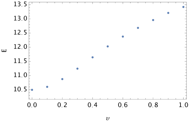
Figure 2: Plot of the energy as a function of $\nu$ for 4 particles. $\tilde{\lambda}$ is equal to 0.5. The simulation is performed at a temperature of $\tilde{\beta}=1$. We used $P=12$ beads and $2\times 10^{7}$ MD steps to assure convergence. The statistical fluctuations are negligible for independent calculations. Hence, we did not give error bar in all our figures.

As a first test, we apply our method for general anyons by varying the parameter $\nu$ from 0 (bosons) to 1 (fermions), and plot the energy as a function of $\nu$, as shown in Fig. 2 for $N=4$ particles. We used a nonzero interaction between particles to reduce sign problem HirshbergFermi ; Dornheim . The energies calculated are taken to be the real part of the complex average energy estimator presented above. The imaginary part of the energy estimator provides an indication for the accuracy of our simulations, a small imaginary part implies that our energy estimation is accurate. In all our simulations in this work, the imaginary part of the energy estimator is negligible. In our simulations, $|{ImE/ReE}|<0.002$. At $\nu=1$ for fermions, our result agrees with the numerical result in Ref. HirshbergFermi based on PIMD. Hence, our simulations are correct in the whole region from bosons to fermions.

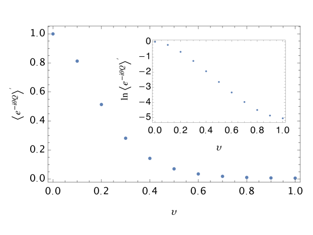
Figure 3: Plot of the magnitude of $\left<e^{-i\theta Q}\right>^{\prime}$ as a function of $\nu$ for 4 particles. For bosons ($\nu=0$) $\left<e^{-i\theta Q}\right>^{\prime}$ is always 1.0. As we increase $\nu$, the magnitude of $\left<e^{-i\theta Q}\right>^{\prime}$ continuously drops to a small number, fermions ($\nu=1$) correspond to the smallest magnitude and most severe sign problem. The inset for $\ln\left<e^{-i\theta Q}\right>^{\prime}$ shows that $\left<e^{-i\theta Q}\right>^{\prime}$ decreases exponentially with increasing $v$.

In order to provide a further investigation into sign problem, we also plot the magnitude of $\left<e^{-i\theta Q}\right>^{\prime}$ as a function of $\nu$, as shown in Fig. 3. A smaller magnitude means that the sign problem is more severe, and more MD iterations are needed to achieve convergence. We found that the sign problem is especially severe for larger number of particles and lower temperatures. To assure the accuracy, we used $2\times 10^{7}$ MD steps for importance sampling, and more MD steps were used to check the convergence.

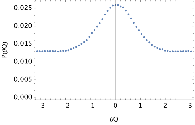
Figure 4: Distribution of the angle $\theta Q$, from $-\pi$ to $\pi$, for interacting fermions with $\tilde{\lambda}=0.5$.

We also plot the distribution of the angle $\theta Q$. For fermions with non-zero interaction, the distribution takes the form of a symmetric and Gaussian function, as illustrated in Fig. 4. In fact, the symmetric probability distribution of $\theta Q$ is the inevitable outcome of the path integral formalism of the partition function given by Eq. (10).

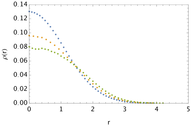
Figure 5: The density function for anyons, normalized to unity. Blue, orange and green represent $\nu=0$, $\nu=0.5$ and $\nu=1.0$ respectively. As $\nu$ increases the peak of the density decreases and the distribution of anyons becomes broader.

Finally, we also investigate the density function for anyons. As $\nu$ increases from 0 to 1, the energy increases, and therefore the density should become broader because of Pauli exclusion principle. This phenomenon is shown in Fig. 5.

IV Calculation of the energy of fermions by anyon model

For anyon systems, it is clear that the sign problem becomes more severe with the increasing of $\nu$ between $0\leq\nu\leq 1$. In Fig. 3, it is shown clearly that $\left<e^{-i\theta Q}\right>^{\prime}$ decreases exponentially with increasing $v$, which leads to the sign problem ceperley ; loh ; troyer ; lyubartsev ; vozn ; Yao1 ; Yao2 ; Yao3 . In our numerical simulations, we can calculate more accurately the energy for $0\leq\nu\leq 0.5$, while less accurately for $\nu\geq 1/2$ (in particular $\nu=1$ for fermions) because of the sign problem. Another numerical inaccuracy in our simulations lies in the approximate calculation of $Q$. Nevertheless, it is expected that $E(\nu)$ is an analytical function of $\nu$ for finite number of particles. When numerical simulation is considered, the analyticity of $E(\nu)$ may require finite temperature so that $P$ is finite. In the thermodynamic limit or zero temperature with infinite $P$, because there are infinite number of beads, we can not assure the analyticity of $E(\nu)$. Of course, it is not necessary to worry about this in practical numerical simulation with finite number of beads. Hence, a reasonable fitting of $E(\nu)$ for small $\nu$ may give us accurate result for the energy of fermions $E(\nu=1)$.

From the partition function for anyons, it is quite interesting to notice that $E(\nu)$ is a periodic function Myrheim of $\nu$ with period $2$. From the symmetry analysis, we also have $E(\nu)=E(-\nu)$. In addition, it is a monotonically increasing function of $\nu$ for $0\leq\nu\leq 1$ because of different exchange forces between bosons and fermions. The exchange forces for fermions are repulsive, while the exchange forces for bosons are attractive. This suggests the following simple function for $E(\nu)$.

$$E(\nu)=E(\nu=0)+a\left[\sin\left(\frac{\pi\nu}{2}\right)\right]^{b}.$$ (31)

Here $a$ and $b$ are two positive real numbers for fitting. The choice of $\sin\left(\frac{\pi\nu}{2}\right)$ in the above expression is due to the general consideration of $E(\nu)$.

Because small value of $\nu$ has less severe sign problem, we may consider to calculate $E(\nu)$ below a value $\nu_{c}$, and use the above function to fit the data to get $E(\nu)$ for fermions with $\nu=1$. For the same parameters in Fig. 2, we use the numerical results of $E(0)$, $E(0.1)$, $E(0.2)$, $E(0.3)$, $E(0.4)$, $E(0.5)$ for data fitting. In Fig. 6(a), the solid line is the best fitting with function (31). We do find that the fitting can give accurate energy for fermions, while suffering from much less severe sign problem. The error of the fitting for the fermions is $2\%$, compared with the result of direct numerical simulation. If the whole region is considered, the mean deviation is smaller than $1\%$.

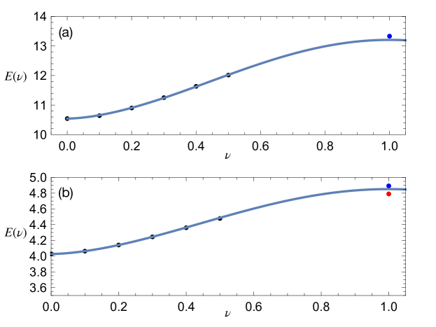
Figure 6: (a) For 4 interacting anyons with the same parameters of Fig. 2, the solid line illustrates the fitting with the data shown by black circles. The blue circle gives the numerical result of $E(\nu=1)$ for fermions, which agrees with the extrapolation in our fitting. (b) For two ideal anyons in a harmonic trap, the solid line shows the fitting of the data shown by black circles in our numerical simulation. As a comparison, the blue circle is the result of numerical simulation, while the red circle is the exact result. We see that the fitting to get the energy of fermions agrees better with the red circle. The slight difference is due to the numerical error in calculating $e^{-i\theta Q}$.

To test further our idea, we also consider here two ideal anyons which have analytical result for the partition function. We consider here two anyons in a two-dimensional harmonic trap $\frac{1}{2}m\omega^{2}(x^{2}+y^{2})$. In unit of $\hbar\omega$ and with the parameter $\tilde{\beta}=1$, in Fig. 6(b), the black circles give the average energy $E(\nu)$ as a function of $\nu$. As expected, we see a monotonic increase of the energy from $\nu=0$ for bosons to $\nu=1/2$ for anyons. For this anyon model, we have analytical result of the energy spectrum. The analytical result of the partition function is Myrheim

$$Z(\beta,\nu)=\frac{\cosh((1-\nu)\beta)}{8\sinh^{2}(\frac{\beta}{2})\sinh^{2}\beta}.$$ (32)

The solid line in Fig. 6(b) gives the average energy based on the fitting with function (31). The red circle gives the energy of two fermions based on the analytical result of the partition function, which agrees well with the extrapolation of our fitting. The error of the fitting for the fermions is $1\%$, compared the exact analytical result. If the whole region is considered, the mean deviation is smaller than $0.5\%$. The slight difference is due to the systematic error of the numerical error of $Q$ because of the discretization in imaginary time and the function for fitting. In the limit of zero temperature, the derivative of $E(\nu)$ about $v$ is nonzero Myrheim at $v=0$ and $v=1$, which is different from the situation of PIMD simulation with finite number of beads. Hence, we should consider carefully the validity of PIMD for zero temperature, when the practical application of our method is considered.

The above two examples show that we have hope to calculate the energy of fermions by anyon models with less severe sign problem. Of course, the present idea can not be applied to large fermion systems because in this case, there are still insurmountable obstacles due to the sign problem even for small $\nu$.

V summary and discussion

In this work we showed how to extend traditional PIMD simulations chandler ; Parrinello ; Tuckerman ; Hirshberg ; HirshbergFermi ; Miura ; Cao ; Cao2 ; Jang2 ; Ram ; Poly ; Craig ; Braa ; Haber ; Thomas to enable the studies of general anyons. Through simple modifications of various physical estimators, we are able to extract physical quantities from simulations for a system of identical interacting anyons. Our methodology may be easily extended to study realistic physical systems of anyons with more complex interactions. We look forward to the applications of PIMD for anyons in the exciting field of many-body quantum systems.

By developing a numerical algorithm for anyons, we also provide further insights into the fermion sign problem. Using the extra freedom in choosing the statistics parameter $\nu$, combined with the choice of interaction parameters, we may extrapolate regime in which the sign problem is less severe into regime with most severe sign problem HirshbergFermi ; DornheimMod (i.e. weakly interacting fermions), hopefully attenuating the fermion sign problem further. Although the present method based on anyon models can not be applied to large fermion system, our work suggests that we may consider to construct more appropriate fictitious particle XiongSFP with a parameter to connect bosons and fermions, similarly to anyon models connecting continuously bosons and fermions.

Acknowledgements This work is partly supported by the National Natural Science Foundation of China under grants number 11175246, and 11334001.

DATA AVAILABILITY

The data that support the findings of this study are available from the corresponding author upon reasonable request. The code of this study is openly available in GitHub (https://github.com/xiongyunuo/PIMD-Anyon).

References

References

- (1) J. M. Kosterlitz and D. J. Thouless, Metastability and Phase Transitions in Two Dimensional Systems, J. Phys. C 6, 1181 (1973).
- (2) Z. Hadzibabic, P. Krüger, M. Cheneau, B. Battelier, and J. Dalibard, Berezinskii-Kosterlitz-Thouless crossover in a trapped atomic gas, Nature 41, 1118 (2006).
- (3) J. M. Leinaas and J. Myrheim, On the theory of identical particles, Il Nuovo Cimento B. 37, 1 (1977).
- (4) F. Wilczek, Magnetic Flux, Angular Momentum, and Statistics, Phys. Rev. Lett. 48, 1144 (1982).
- (5) F. Wilczek, Quantum Mechanics of Fractional-Spin Particles, Phys. Rev. Lett. 49, 957 (1982).
- (6) F. Wilczek, Fractional Statistics and Anyon Superconductivity (World Scientific, Teaneck, 1990).
- (7) A. Khare, Fractional Statistics and Quantum Theory (World Scientific, Singapore, 2005).
- (8) D. C. Tsui, H. L. Stormer, and A. C. Gossard, Two-Dimensional Magnetotransport in the Extreme Quantum Limit, Phys. Rev. Lett. 48, 1559 (1982).
- (9) H. Bartolomei, et al., Fractional statistics in anyon collisions, Science 368, 173 (2020).
- (10) J. Nakamura, S. Fallahi, H. Sahasrabudhe, R. Rahman, S. Liang, G. C. Gardner, and M. J. Manfra, Aharonov-Bohm interference of fractional quantum Hall edge modes, Nat. Phys. 15, 563 (2019).
- (11) J. Nakamura, S. Liang, G. C. Gardner, and M. J. Manfra, Direct observation of anyonic braiding statistics, Nat. Phys. 16, 931 (2020).
- (12) R. P. Feynman and A. R. Hibbs, Quantum Mechanics and Path Integrals (Dover Publications, New York, 2010).
- (13) H. Kleinert, Path Integrals in Quantum Mechanics, Statistics, Polymer Physics, and Financial Markets (World Scientific, Singapore, 2009).
- (14) D. M. Ceperley, Path integrals in the theory of condensed helium, Rev. Mod. Phys. 67, 279 (1995).
- (15) M. Boninsegni, N. V. Prokofev, and B. V. Svistunov, Worm algorithm and diagrammatic Monte Carlo: A new approach to continuous-space path integral Monte Carlo simulations, Phys. Rev. E 74, 036701 (2006).
- (16) M. Boninsegni, N. V. Prokofev, and B. V. Svistunov, Worm Algorithm for Continuous-Space Path Integral Monte Carlo Simulations, Phys. Rev. Lett. 96, 070601 (2006).
- (17) T. Dornheim, The Fermion Sign Problem in Path Integral Monte Carlo Simulations: Quantum Dots, Ultracold Atoms, and Warm Dense Matter, Phys. Rev. E 100, 023307 (2019).
- (18) D. Chandler and P. G. Wolynes, Exploiting the isomorphism between quantum theory and classical statistical mechanics of polyatomic fluids, J. Chem. Phys. 74, 4078 (1981).
- (19) M. Parrinello and A. Rahman, Study of an F center in molten KCl, J. Chem. Phys. 80, 860 (1984).
- (20) M. E. Tuckerman, Statistical Mechanics: Theory and Molecular Simulation (Oxford University, New York, 2010).
- (21) B. Hirshberg, V. Rizzi, and M. Parrinello, Path integral molecular dynamics for bosons, Proc. Natl. Acad. Sci. U. S. A. 116, 21445 (2019).
- (22) Y. N. Xiong and H. W. Xiong, Path integral molecular dynamics simulations for Green’s function in a system of identical bosons, J. Chem. Phys. 156, 134112 (2022).
- (23) Y. L. Yu, S. J. Liu, H. W. Xiong, and Y. N. Xiong, Path integral molecular dynamics for thermodynamics and Green’s function of ultracold spinor bosons, arXiv:2207.07653 (2022).
- (24) B. Hirshberg, M. Invernizzi, and M. Parrinello, Path integral molecular dynamics for fermions: Alleviating the sign problem with the Bogoliubov inequality, J. Chem. Phys. 152, 171102 (2020).
- (25) Y. N. Xiong and H. W. Xiong, Numerical calculation of Green’s function and momentum distribution for spin-polarized fermions by path integral molecular dynamics, J. Chem. Phys. 156, 204117 (2022).
- (26) D. M. Ceperley, Path Integral Monte Carlo Methods for Fermions, Monte Carlo and Molecular Dynamics of Condensed Matter Systems, K. Binder and G. Ciccotti (Eds.), Bologna (Italy) (1996).
- (27) E. Y. Loh, J. E. Gubernatis, R. T. Scalettar, S. R. White, D. J. Scalapino, and R. L. Sugar, Sign problem in the numerical simulation of many-electron systems, Phys. Rev. B 41, 9301 (1990).
- (28) M. Troyer and U. J. Wiese, Computational Complexity and Fundamental Limitations to Fermionic Quantum Monte Carlo Simulations, Phys. Rev. Lett. 94, 170201 (2005).
- (29) A. P. Lyubartsev, Simulation of excited states and the sign problem in the path integral Monte Carlo method, J. Phys. A: Math. Gen. 38, 6659 (2005).
- (30) M. A. Voznesenskiy, P. N. Vorontsov-Velyaminov, and A. P. Lyubartsev, Path-integral-expanded-ensemble Monte Carlo method in treatment of the sign problem for fermions, Phys. Rev. E 80, 066702 (2009).
- (31) Z. X. Li, Y. F. Jiang, and H. Yao, Solving the fermion sign problem in quantum Monte Carlo simulations by Majorana representation, Phys. Rev. B 91, 241117(R) (2015).
- (32) Z. X. Li, Y. F. Jiang, and H. Yao, Majorana-Time-Reversal Symmetries: A Fundamental Principle for Sign-Problem-Free Quantum Monte Carlo Simulations, Phys. Rev. Lett. 117, 267002 (2016).
- (33) Z. X. Li and H. Yao, Sign-Problem-Free Fermionic Quantum Monte Carlo: Developments and Applications, Ann. Rev. Cond. Mat. Phys. 10, 337 (2019).
- (34) J. Myrheim, in Anyons edited by A. Comtet, T. Jolicoeur, S. Ouvry, and F. David (Springer-Verlag, 1999), 69, pp. 265-413.
- (35) S. Nosé, A molecular dynamics method for simulations in the canonical ensemble, Mol. Phys. 52, 255 (1984).
- (36) S. Nosé, A unified formulation of the constant temperature molecular dynamics methods, J. Chem. Phys. 81, 511 (1984).
- (37) W. G. Hoover, Canonical dynamics: Equilibrium phase-space distributions, Phys. Rev. A 31, 1695 (1985).
- (38) G. J. Martyna, M. L. Klein, and M. Tuckerman, Nosé-Hoover chains: The canonical ensemble via continuous dynamics, J. Chem. Phys. 97, 2635 (1992).
- (39) Mark E. Tuckerman and Bruce J. Berne, Efficient molecular dynamics and hybrid Monte Carlo algorithms for path integrals, J. Chem. Phys. 99, 2796 (1993).
- (40) S. Jang and G. A. Voth, Simple reversible molecular dynamics algorithms for Nosé-Hoover chain dynamics, J. Chem. Phys. 107, 9514 (1997).
- (41) S. Miura and S. Okazaki, Path integral molecular dynamics for Bose-Einstein and Fermi-Dirac statistics. J. Chem. Phys. 112, 10116 (2000).
- (42) J. Cao and G. A. Voth, The formulation of quantum statistical mechanics based on the Feynman path centroid density. I. Equilibrium properties, J. Chem. Phys. 100, 5093 (1994).
- (43) J. Cao and G. A. Voth, The formulation of quantum statistical mechanics based on the Feynman path centroid density. II. Dynamical properties, J. Chem. Phys. 100, 5106 (1994).
- (44) S. Jang and G. A. Voth, A derivation of centroid molecular dynamics and other approximate time evolution methods for path integral centroid variables, J. Chem. Phys. 111, 2371 (1999).
- (45) R. RamíRez and T. LóPez-Ciudad, The Schrödinger formulation of the Feynman path centroid density, J. Chem. Phys. 111, 3339 (1999).
- (46) E. A. Polyakov, A. P. Lyubartsev, and P. N. Vorontsov-Velyaminov, Centroid molecular dynamics: Comparison with exact results for model systems, J. Chem. Phys. 133, 194103 (2010).
- (47) I. R. Craig and D. E. Manolopoulos, Quantum statistics and classical mechanics: Real time correlation functions from ring polymer molecular dynamics, J. Chem. Phys. 121, 3368 (2004).
- (48) B. J. Braams and D. E. Manolopoulos, On the short-time limit of ring polymer molecular dynamics, J. Chem. Phys. 125 ,124105 (2006).
- (49) S. Habershon, D. E. Manolopoulos, T. E. Markland, and T. F. Miller 3rd, Ring-polymer molecular dynamics: quantum effects in chemical dynamics from classical trajectories in an extended phase space, Annu. Rev. Phys. Chem. 64, 387 (2013).
- (50) T. E. Markland and M. Ceriotti, Nuclear quantum effects enter the mainstream, Nat. Rev. Chem. 2, 0109 (2018).
- (51) T. Dornheim, M. Invernizzi, J. Vorberger, and B. Hirshber, Attenuating the fermion sign problem in path integral Monte Carlo simulations using the Bogoliubov inequality and thermodynamic integration, J. Chem. Phys. 153, 234104 (2020).
- (52) Y. N. Xiong and H. W. Xiong, A solution of fermion sign problem for large fermion systems, arXiv:2206.08341 (2022).