Estimating Peak-Hour Traffic Congestion Patterns For Interacting Agents On Urban Networks

Abstract

We study the emergence of congestion patterns in urban networks by modeling vehicular interaction by means of a simple traffic rule and by using a set of measures inspired by the standard Betweenness Centrality (BC). We consider a topologically heterogeneous group of cities and simulate the network loading during the morning peak-hour by increasing the number of circulating vehicles. At departure, vehicles are aware of the network state and choose paths with optimal traversal time. Each added path modifies the vehicular density and travel times for the following vehicles. Starting from an empty network and adding traffic until transportation collapses, provides a framework to study network’s transition to congestion and how connectivity is progressively disrupted as the fraction of impossible paths becomes abruptly dominant. We use standard BC to probe into the instantaneous out-of-equilibrium network state for a range of traffic levels and show how this measure may be improved to build a better proxy for cumulative road usage during peak-hours. We define a novel dynamical measure to estimate cumulative road usage and the associated total time spent over the edges by the population of drivers. We also study how congestion starts with dysfunctional edges scattered over the network, then organizes itself into relatively small, but disruptive clusters.

I Introduction

Urban networks have been widely studied in recent years [1, 2, 3], both their growth over time and their complex dynamics under different traffic levels. Network science has considerably helped to improve our understanding of cities and to analyze and predict the reaction of the different parts of the network under stress [4, 5]. Such predictive analyses may be performed by considering just the geographical and topological features of a city, without having to recur to experimental traffic data, but these datasets constitute nonetheless the reference against which every theoretical model should be evaluated [6, 7]. Urban networks belong to the special class of (almost) planar graphs and in this context there have been some notable results recently [8, 9]. The geographical embedding leads to several constraints to topology such as limitations to the number of long-range connections and to the maximum connectivity observed at the single edge level [10]. The study of edge degree distributions did not improve much our understanding of cities, but non-local higher-order metrics such as network centralities have been widely used both for theoretical studies and for practical applications with notable success [11, 12]. One of the metrics that have been used the most in recent years is the Betweenness Centrality (BC), which is defined as the total flow passing over each node of the network when enumerating all Origin-Destination (OD) pairs and connecting them via shortest-path routing. This definition is easily extended to Edge BC (EBC) by counting edge usage instead. We will write BC instead of EBC in the rest of paper since our focus will be on edges. BC and other measures have been used to predict which edges are subject to the highest traffic demand that leads to the breakup of the network into functionally independent pieces. This phase transition has been well studied via percolation theory and it is known that the size distribution of the resulting sub networks follows a power law with a critical exponent that depends on traffic intensity and on the time of the day. This transition has been observed for real world datasets in large cities such as London, Beijing and New York City [13, 4, 14]. During the most extreme conditions, total network breakdown has been observed to last for several hours or even days [5].

The percolation phase transition is not specific of high congestion levels, but an edge may be classified as dysfunctional even with vehicles traveling just below the speed limit [2, 4, 13]: this transition simply signals a change in the network behavior that happens at all traffic levels, but for different critical speeds. On the other hand, in this work we will follow the more practical definition of calling an edge dysfunctional only when it cannot receive traffic anymore, due to road density nearing the maximum value and speed approaching zero [5]. The transition happens when there is suddenly a large part of the desired travel paths that are no longer usable.

Standard BC approaches can only grasp a limited picture of the network under stress because BC relies on several assumptions [15, 16]: traffic origins and destinations uniformly spread over the nodes; shortest paths with fixed cost function; non-interacting multiple paths sharing the same edge; the amount of traffic density contributed by each vehicle is the same regardless of its driving time. Edge usage obtained from a BC computation approximates well a network with very small (or extremely fast) agents, each using shortest path navigation with no congestion awareness [17]. A urban transportation network is characterized by vehicle travel times comparable to the typical timescale of congestion buildup during peak-hours.

In this work we want to extend the standard BC as a measure of road congestion, especially by taking into account the strong interaction effects observed in real traffic. The interaction among vehicles depends on the duration and vehicular volume of the network loading: the longer the edge travel times, the higher the probability of finding a vehicle in a given road segment during the observation period. The present approach stems directly from this fact and aims at focusing on the peak-hour periods, that usually last for one hour, to estimate the cumulative traffic seen on the roads during that finite time window. Thus, we propose a dynamical model to compute the contribution to traffic at a road-segment level due to each vehicle added to the network, while iteratively recomputing travel times after each addition. From the vast literature on transportation we choose one of the simplest models to describe vehicular behavior depending on geography (edge properties) and on the dynamical network state: the single regime Greenshields model [9, 18], for which speed starts at the free flow value to decrease linearly to zero when maximal road density is attained. To complement the traffic model, we assume that vehicles know exactly the network state before their departure, in order to plan an optimal path. The proposed scenario mimics a network with a mixture of self-driving cars and human drivers generating a shortest-time route at the start of their trips. It is likely that this will become increasingly relevant in the near future.

In this paper we employ our dynamical model and the associated metrics to theoretically predict the behavior of five large cities under growing traffic. Results will be validated against real traffic data in future works.

II Methods

II.1 Interaction Model

We aim at modeling the network evolution, as observed by travelers, while the traffic increases from zero up to complete gridlock. The desired network traffic over simulation time ($\tau$) will be added incrementally, activating one new path $\pi(i)$ at each simulation step $i$. Thus, $i$ can be interpreted both as the current number of added paths and as a temporal marker to define the sequence of OD pairs randomly generated for each simulation.

For simplicity, and to be able to compare results with the standard BC, traffic will be added uniformly to the network. It is however straightforward to adapt our procedure to any OD matrix.

We model the traffic network as a directed, weighted graph $G=(V,E)$ with $N=|V|$ nodes and $M=|E|$ edges. Each edge $e$ represents a road segment between two intersections and it is characterized by three constant features: its physical length $l_{e}$, maximum speed $v^{*}_{e}$ and number of lanes $c_{e}$.

The state of the network at each time step will be represented by the occupancy of vehicles added so far in each edge ${s_{e}(i)}$, where $s_{e}(i)=\sum_{j=1}^{i}\sigma_{e}(j)$. We will define the occupancy $\sigma$ of a single vehicle so that it will sum to one only when its total traveling time is equal to or longer than the simulation time (in general: $\sum_{e\in\pi(i)}\sigma_{e}(i)\leq 1$). To each edge we also associate a normalized vehicle density $\rho_{e}(i)$, that increases monotonically as we add vehicles:

$$\rho_{e}(i)=\frac{s_{e}(i)L}{l_{e}c_{e}}\in[0,1]\operatorname{\enspace,}$$ (1)

where $L$ is the average space occupied by one vehicle.

We define the occupancy $\sigma_{e}(i)$ of a new vehicle added to the network using a simple approximation of the time it might spend on edge $e$:

$$\sigma_{e}(i) =\min\left(\frac{T_{e}(i)}{\tau},1\right)\operatorname{\enspace,} \text{where }T_{e}(i) =\frac{l_{e}}{v_{e}(i)}\operatorname{\enspace,}$$ (2)

and with speed $v_{e}(i)$ following a Greenshields linear law [19]:

$$v_{e}(i)=v_{e}^{*}(1-\rho_{e}(i-1))\operatorname{\enspace,}$$ (3)

thus the approximate time for the complete path $\pi(i)$ will be $T_{\pi(i)}=\sum_{e\in\pi(i)}T_{e}(i)$. A non-interacting system is obtained in the limit $L\rightarrow 0$. In more detail, the state $s(i)$ of the network is obtained iteratively ($s(i)=f(s(i-1))$), starting with an empty network ($s(0)=0$) and according to the following dynamic process:

• a pair of OD nodes is chosen, independently and uniformly at random, and the fastest path $\pi(i)$ connecting the nodes is computed;

• starting from O, for each edge $e\in\pi(i)$, we accumulate the average occupancy $\sigma(i)$ induced by $\pi(i)$ during $\tau$:

  $$s_{e}(i)=s_{e}(i-1)+\sigma_{e}(i)\operatorname{\enspace,}$$ (4)

  and the number of vehicles on the edge:

  $$n_{e}(i)=n_{e}(i-1)+1\operatorname{\enspace.}$$ (5)

  Note that, as soon as the sum along $\pi(i)$ of the added $T_{e}(i)/\tau$ factors reaches $1$, we choose to skip the remaining edges up to D, to avoid adding more than a unit factor to vehicle occupancy along $\pi(i)$;

• $v_{e}(i+1)$ and $T_{e}(i+1)$ are updated according to Eqs. 2 and 3, using the new $\rho_{e}(i)$ value;

• this process is iterated until the desired total traffic is reached.

Intuitively, the occupancy factor induced by a vehicle over an edge $e$ is proportional to the time the vehicle is supposed to spend on it (${T_{e}}/{\tau}$), as forecast at the moment of its generation, and the sum over the whole path will be equal to unity (certainty of finding the vehicle within $\pi$ during $\tau$) only when $T_{\pi}\geq\tau$. The initial OD pairs find a nearly empty network, so their fastest paths and travel times are very similar to the $L=0$ case. With rising traffic, however, edges slow down and subsequent fastest paths will be slower and, in general, different. Some edges will eventually reach maximum density and become dysfunctional. If the fastest route from origin to destination comprises a dysfunctional edge (i.e., the network is disconnected) we still choose to add the initial part of the path, but we will skip the edges starting from the first dysfunctional one. This allows us to model the backward propagation of traffic jams observed at high traffic volumes [20, 14]. Since the order in which OD pairs are added to the network can lead to different final results, we replicate the system and perform several simulations to analyze the stability of the results.

The main limitations of this model are: the Greenshields model is very rough; no explicit time evolution as in the Nagel-Schreckenberg CA model, but just a sequence of path addition in a first come, better served approach; no true time evolution means that long paths added initially will generally experience faster times (uncongested) for edges that will likely become congested later by newer paths; OD pairs are uniformly extracted at random over the network: it is known, e.g., that morning and evening peak hours show an opposite average traffic direction [1].

II.2 Cumulative BC definition

BC implicitly assumes that the different paths do not interact, i.e., that the cost (typically the shortest length between two points) does not change when adding agents in the network. If, however, we assume that the active network traffic does alter the cost function, as it is the case when choosing fastest vs shortest paths, then the standard BC gives a biased picture of bottlenecks and hotspots. A good approximation of the BC can be obtained by sampling the OD pairs uniformly [21], and it is natural to think about it as a dynamical process of subsequent path additions. In particular, if the exact paths, their order of appearance and their travel times are known, the timescale $\tau$ of the dynamical phenomenon becomes a crucial parameter to better estimate the edge visiting frequencies.

Several studies extending the original BC concept have been presented in the past [22, 12, 11], to deviate from the idea of shortest paths by introducing routing randomness. Here, on the other hand, we extend the BC idea by taking into account the evolution of the network state. To this aim, we define a Cumulative BC (CBC), based on the average occupancy $s_{e}(i)$, defined in Eq. 4 as:

$$\gamma_{e}(i)=\frac{s_{e}(i)}{i}\operatorname{\enspace.}$$ (6)

This quantity is normalized and tends to the original BC for $L\rightarrow 0$.

III Simulation details

We select the vehicular transportation layer of the urban networks relative to five large cities and their surroundings from OpenStreetMap. The radius $R$ of the circle inscribed in each region varies from $12$ km for Rome to $20$ km for Boston, and the number of edges of the corresponding graphs ranges from about 65k of Rome to about 200k of London. For every city, we perform $10$ simulations, each with a reshuffled order of the OD additions to the network to estimate the sensitivity of the evolving configurations to external conditions. The total number of added ODs was $10^{6}$, sufficient to bring all cities to a deeply congested state. The total computation time for simulation and analysis is less than one day for each city, running with shared-memory parallelism on Intel E5-2680 nodes (12 cores, 2 threads/core) with 250 GB RAM.

IV Results and discussions

IV.0.1 Transition to fragmented network

We first focus on the behavior of the network while it receives an increasing number of paths. Since edges become progressively dysfunctional as $\rho\rightarrow 1$, at some traffic level (set by $i$) the graph becomes disconnected, which means that some OD pairs will belong to functionally separated subgraphs. When this occurs, all paths connecting those OD pairs will include a dysfunctional edge and we say that the OD pair is (at least partially) rejected. This is a coarse indicator of a transition in the network behavior. We present rejection ratio curves in Fig. 2: Nairobi (Fig. 2a) and Rio (Fig. 2b) are the first to collapse at $i\approx 210$k and $i\approx 320$k, respectively, with moderately steep curves. The different transition types depend upon the topological features of each city (see maps on Fig. 8): London (Fig. 2c) and Rome (Fig. 2d), being traversed by rivers, abruptly break at $i\approx 335$k and $i\approx 490$k, respectively, leaving both cities split in two halves ($50\%$ of rejected ODs). The collapsed bridges of both cities, due to heavy usage, are clearly visible in Fig. 8(c). Once broken in two parts, London is able to better support local traffic better than Rome that collapses quickly even for shorter ODs, as visible from the different slopes after the transition. Boston (Fig. 2e) is apparently the most resilient to breakup, with the first hints of congestion appearing at $i\approx 560$k, and a global behavior similar to Nairobi and Rio.

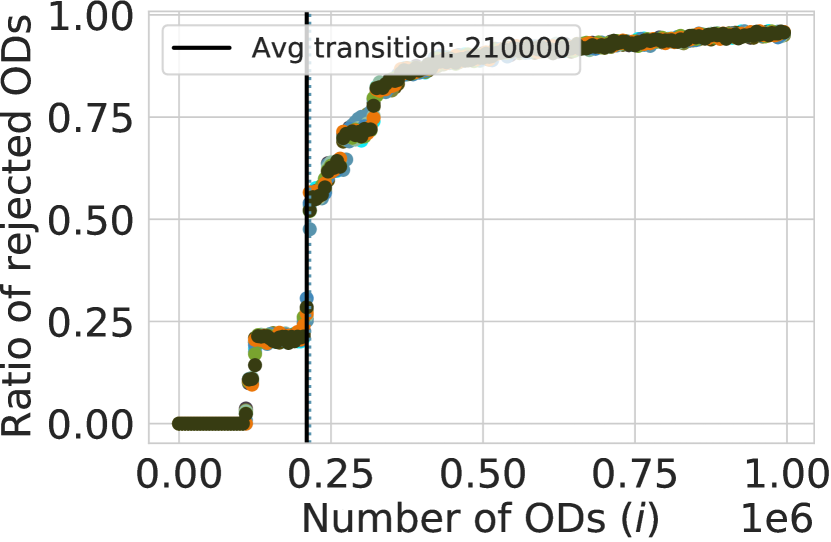
(a) Nairobi

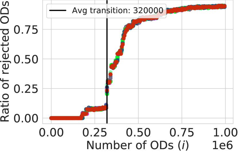
(b) Rio

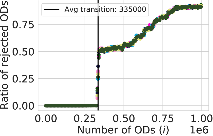
(c) London

(d) Rome

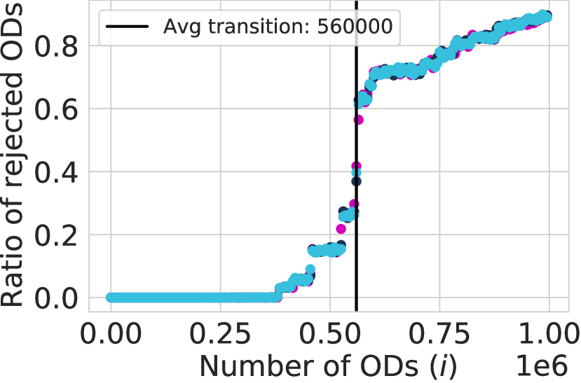
(e) Boston

Figure 2: Fraction of (partially) rejected paths for increasing traffic ($i$)

We now shift our focus to the spatial configuration of dysfunctional edges: to display their typical growth over the graph, we choose Rio in Fig. 4 (left): the number of dysfunctional edges (red curve) and that of edges belonging to the Largest strongly connected dysfunctional Cluster (LC) grow almost monotonically with $i$ (black curve). It is worth noting that, although scattered dysfunctional edges appear early and grow monotonically, the LC lags and shows a staircase-like behavior, indicating that dysfunctional edges take time to coalesce into a set of clusters. We measure only the LC size and the plateaus are explained by new dysfunctional edges appearing in distant parts of the city. Remarkably, the table on the right of Fig. 4 shows that, for all cities, a small number of dysfunctional edges of order $0.1\%$ of the total edges, is enough to severely hinder transportation efficiency.

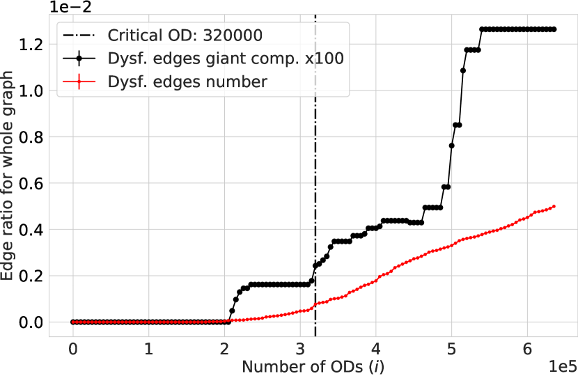
	# dysf.	LC size
Boston	$2\cdot 10^{-3}$	$4\cdot 10^{-5}$
London	$5\cdot 10^{-4}$	$2\cdot 10^{-5}$
Rome	$3\cdot 10^{-3}$	$6\cdot 10^{-5}$
Rio	$1\cdot 10^{-3}$	$3\cdot 10^{-5}$
Nairobi	$1\cdot 10^{-3}$	$9\cdot 10^{-5}$

Figure 4: Spatial correlation of congested edges. Left: Fraction of dysfunctional edges (w.r.t. the entire graph) found at the transition in Rio as traffic increases in red, and in black (magnified $100$ times), the associated largest connected component cluster size fraction. Right: Values of red ($\#$ dysf.) and black (LC size) curves at the transition for each city.

In order to further analyze the transition to congestion, we define two additional measures: the average path length ratio: $\mathbf{D}(i)=\frac{1}{iR}\sum_{e}n_{e}(i)\cdot l_{e}$ and the average path time per vehicle: $\mathbf{T}(i)=\frac{1}{i}\sum_{e}n_{e}(i)\cdot t_{e}$. Since $n_{e}(i)$ is the number of vehicles that chose edge $e$ in $\tau$, by summing its products with edge lengths (traversal times) we obtain the global distance run (time spent) by all vehicles in $\tau$. $\mathbf{D}(i)$, with respect to the traffic level $i$, shows different regimes up to the transition: a constant or gentle slope for London and Rio, respectively, a bit steeper for Boston; a marked peak at the transition for all cities except Nairobi and Boston (Fig. 6); a final decrease, for all cities after the transition, mainly due to partial truncation of paths added after the transition. $\mathbf{T}(i)$ per vehicle are similar for all cities: Fig. 6 (right) shows a gentle slope for low traffic regimes, which suddenly steepens nearing the transition with the dysfunctional edges restricting the choice of optimal paths. For brevity, $\mathbf{D}(i)$ and $\mathbf{T}(i)$ are shown in Fig. 6 only for Boston: as traffic rises, avoidance of congested roads leads to an increase in the average travel length, but in general by less than $\approx 10\%$.

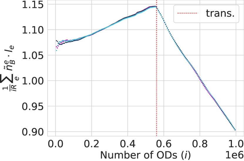
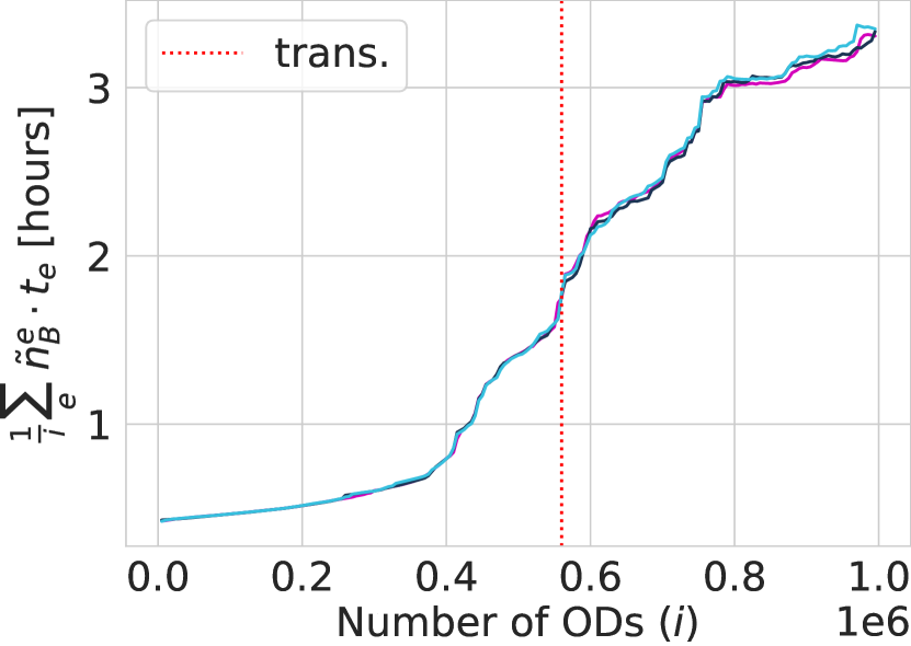
Figure 6: (Average path length ratio $\mathbf{D}(i)$ (with respect to $R$) (left) and path travel time $\mathbf{T}(i)$ (right) per vehicle for Boston. Each color represents a different replica with reshuffled OD order.

IV.0.2 BC at increasing levels of traffic

Standard BC may be used to probe the network state, after the addition of a number of vehicles, to obtain instantaneous information on how congestion affects path choices for increasing traffic levels. Fig. 8 (a) and (b) show how the BC maps of our five cities change from the empty state to the transition. Specifically, in Fig. 8 (b), edges with either larger or lower BC with respect to the empty state, are shown in red and blue respectively. It is worth to note that the roads with the highest BC with little traffic become dysfunctional long before the transition as entirely different path choices emerge: blue roads in Fig. 8 (b) are those that lost most of their flow due to early saturation while the red ones became important at higher congestion levels.

IV.0.3 Cumulative BC

The “loaded” standard BC discussed above, does not describe the network behavior during the whole simulation time, but just what would happen to a small batch of vehicles added on top of a system with a specific traffic load. The Cumulative BC (CBC), on the other hand, takes into account the total contributions of all vehicles added within $\tau$. The CBC maps are shown in Fig. 8(c) exactly at the transition $i_{c}$ specific for each city, so each edge carries the contribution to the global traffic experienced during the whole simulation time. Several edges show high CBC values not detected as important by a BC in Fig. 8 (a). This is especially true for peripheral roads that become important only when the fastest options are already saturated: notably, Boston shows a somewhat busy eastern region and Rome has several radial roads that show a relatively large usage.

IV.0.4 Total Time Spent in Traffic (TS)

After defining the CBC as a proxy for the number of vehicles to be observed during the network loading, we can use this information to obtain some interesting features, such as the total time spent by all vehicles on each edge: $\mathbf{TS}_{e}(i)=\frac{1}{l_{e}}\sum_{e}n_{e}(i)T_{e}(i)$. This measure provides an intuitive way of estimating the total wait experienced, per unit length, during $\tau$ by all vehicles sharing an edge. As visible in Fig. 8(d), the maps show the relative importance of each road: low values belong to seldom used roads while high values emerge for roads that are frequently chosen whether with an empty network (coinciding with BC) or at near-congestion. In general, urban highways, with several lanes and higher speed limits, are the primary candidates to display top scores in this metric, but as congestion grows, other roads, often not planned for heavy use, start to attract a large fraction of vehicles and may compete with highways. It should be noted how most of the top-ranked roads in London are bridges over the Thames that in fact are the first to become dysfunctional (as seen in Fig. 2(c)), leading to a city split in two roughly equal parts.

(a) Standard BC       

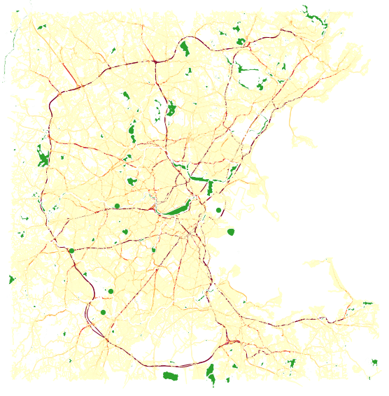
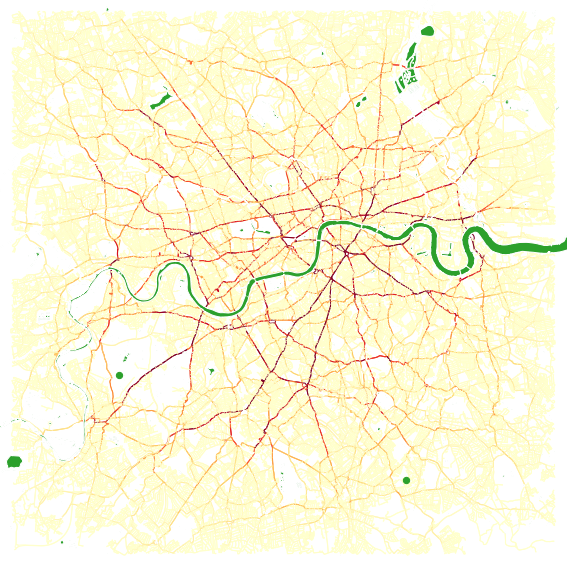
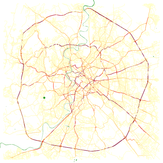
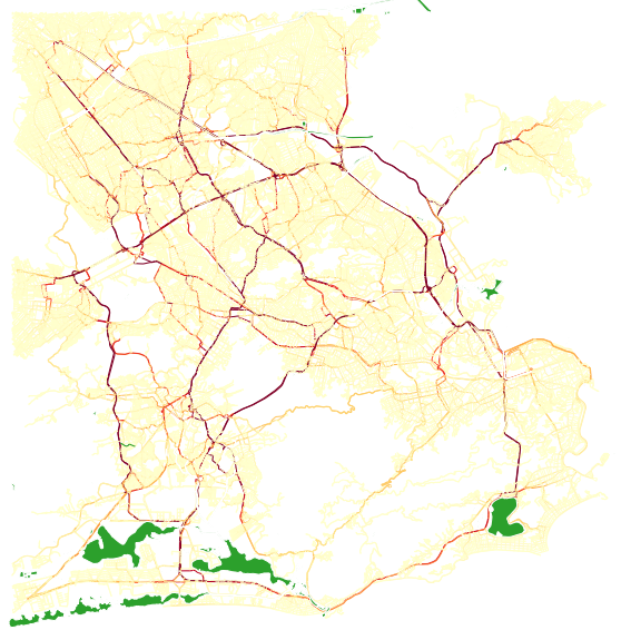
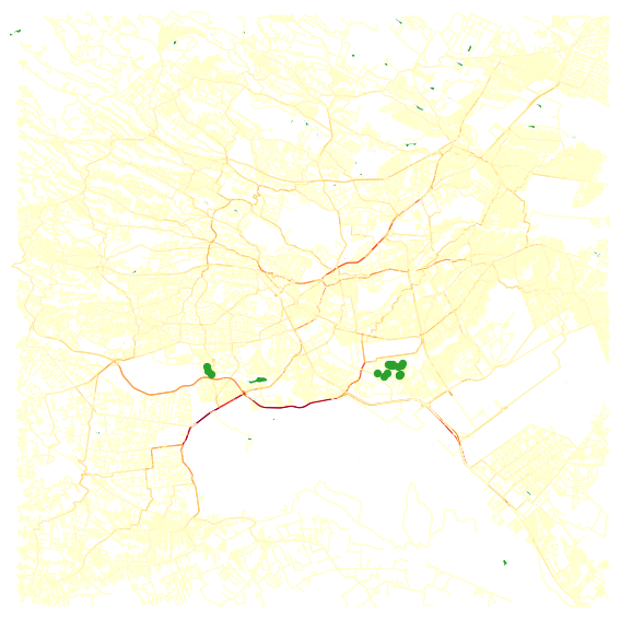
(b) $\Delta BC$       

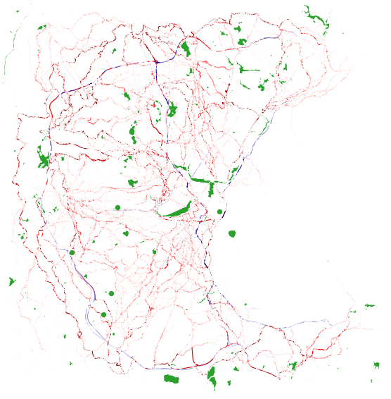
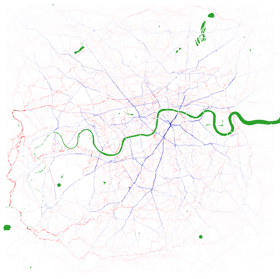
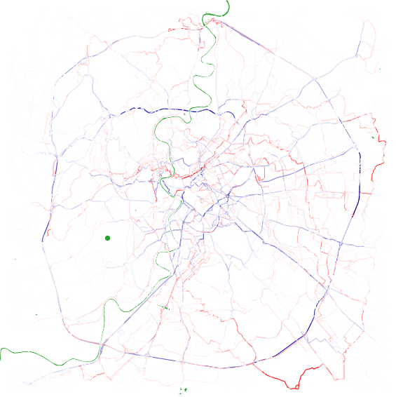
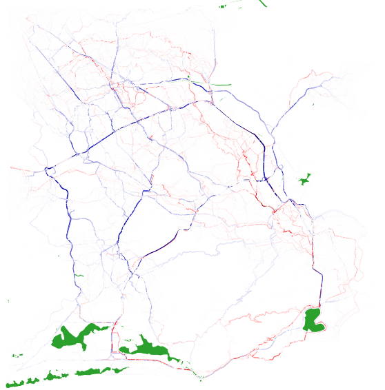
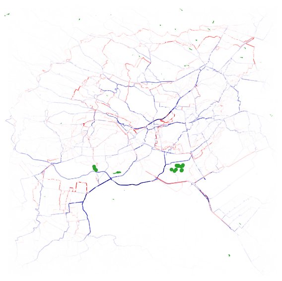
(c) CBC       

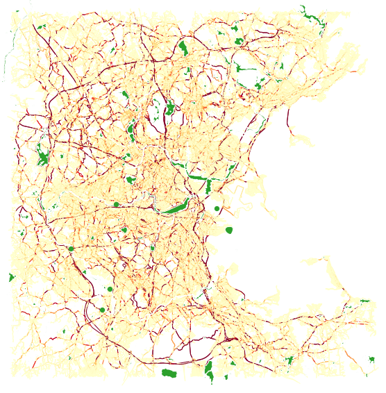
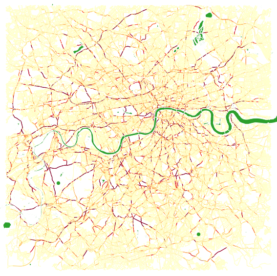
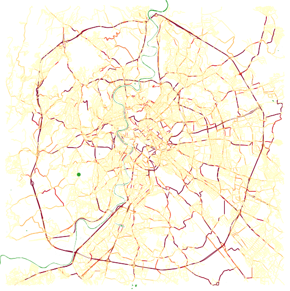
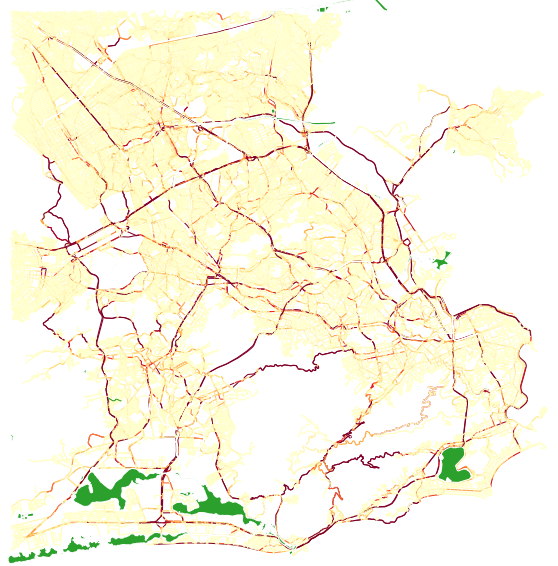
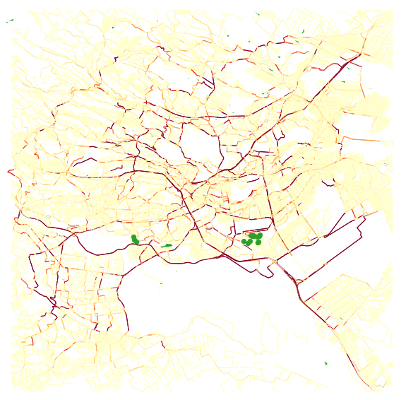
(d) Time Spent       

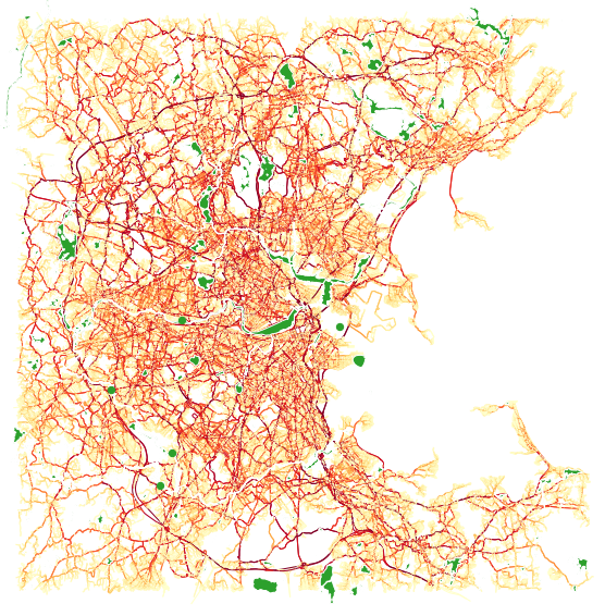
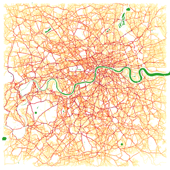
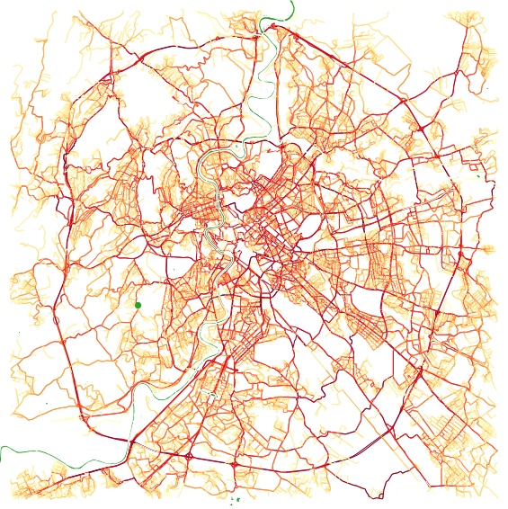
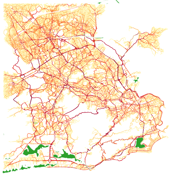
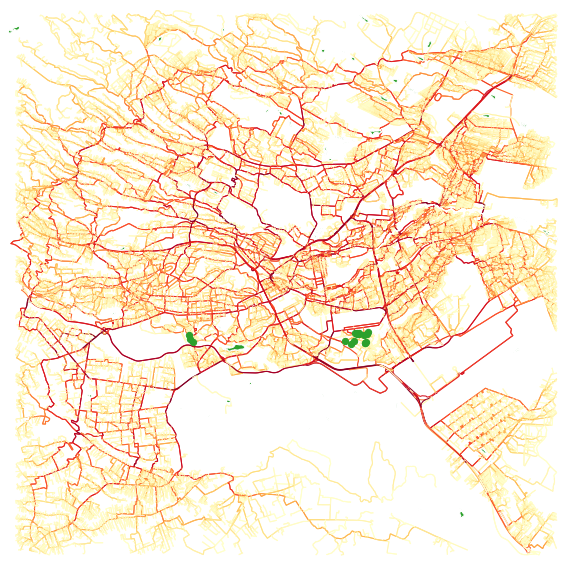
i Boston

ii London

iii Rome

iv Rio

v Nairobi

Figure 8: (a): Standard BC maps for all cities: red edges are within the $99$-th percentile of the BC distribution for the empty network. (b): $\Delta$BC at the transition: deep red and dark blue edges increase or decrease their BC by $\approx 100\%$, respectively. (c): red edges show the $99$-th percentile of the CBC distribution at the transition. (d): red edges represent the $99$-th percentile of the Time Spent in Traffic distribution at transition (per unit length, in order not to visually overestimate longer edges).

IV.0.5 CBC and total time spent in traffic

We study how the distributions of CBC (Fig. 10(a)) and total time spent in traffic (TS) (Fig. 10(b)) change for all cities when traffic grows from light to severely congested. As expected, both distributions shift to the right and a double peak structure starts to emerge already for medium-low traffic levels. The indications of behavior change obtainable from the standard BC in the same conditions are much weaker as seen in [3] as the BC distribution is almost invariant for totally different cities.

(a) CBC       

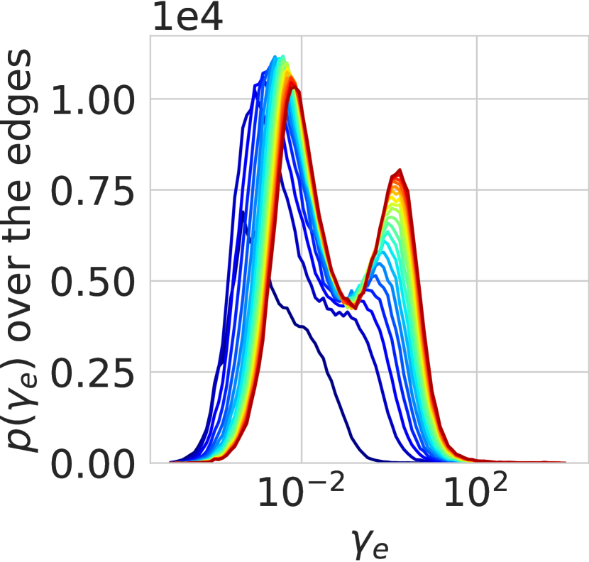
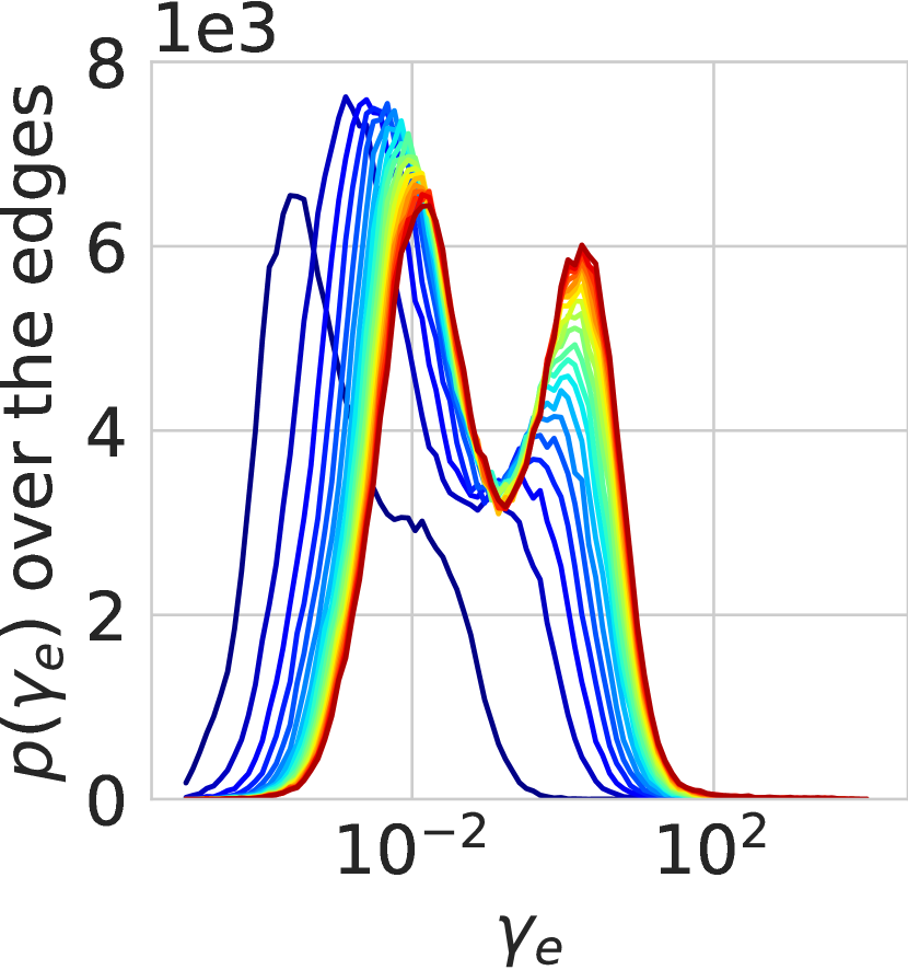
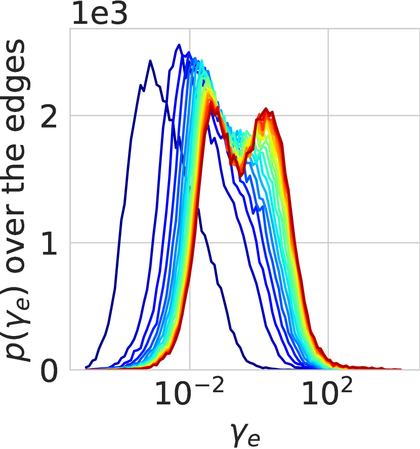
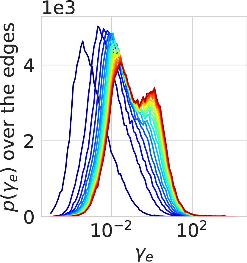
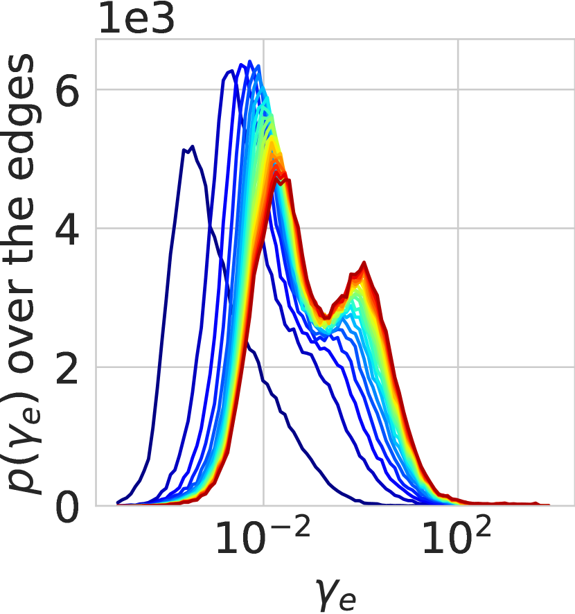
(b) Time Spent       

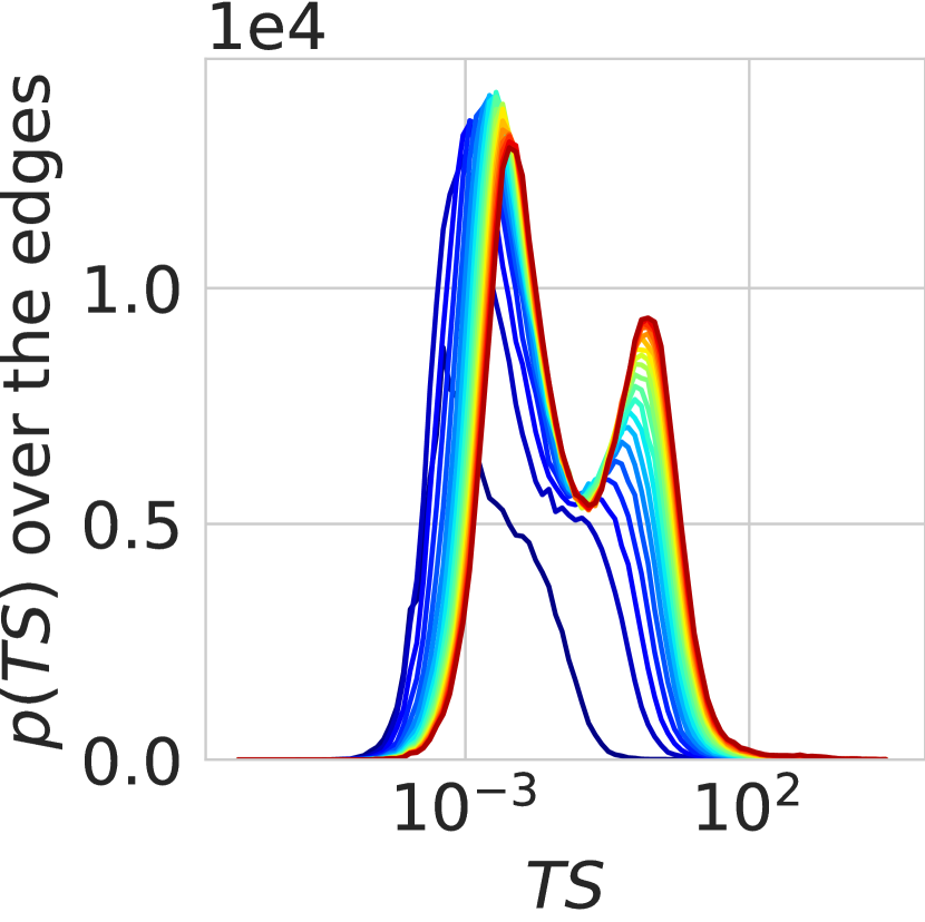
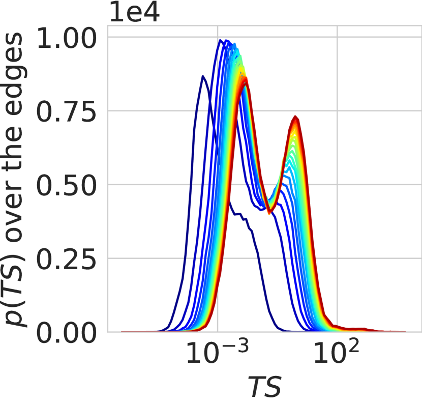
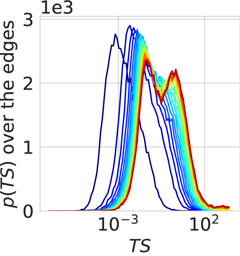
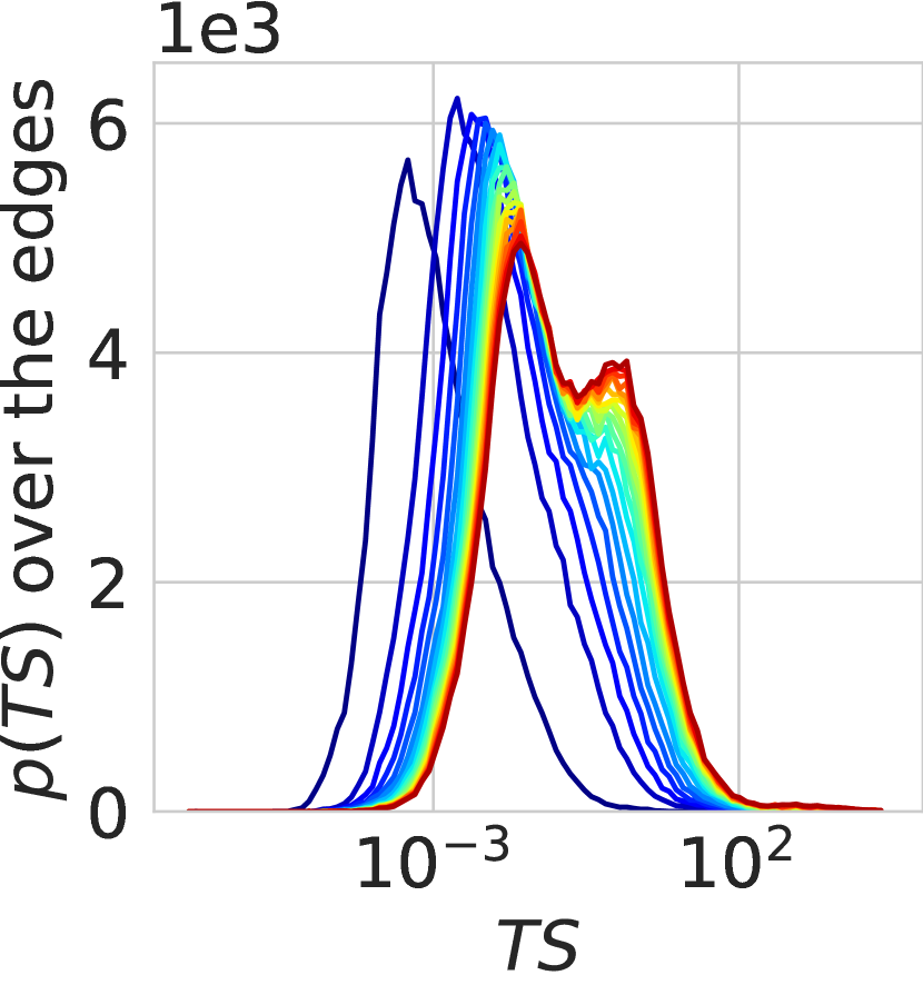
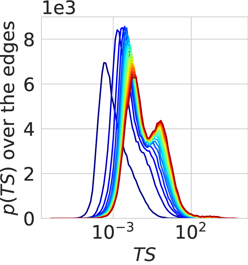
i Boston

ii London

iii Rome

iv Rio

v Nairobi

Figure 10: Top: CBC [average occupancy per edge in 1h] for all cities at increasing levels of traffic (blue: light traffic, green: near transition, red: congested). Bottom: Time Spent in Traffic (TS) [vehicles$\cdot$hour]. Colors as for top row.

V Conclusion

By extending the idea of BC, we proposed a novel approach based on a dynamical model to take into account interactions among vehicles, to specifically characterize the peak-hour network loading, typically the most demanding time in terms of infrastructural stress. Our results show that the Cumulative BC is able to identify the bottlenecks of the network, when subjected to a persistent load, and to study the back-propagation of traffic jams. Interpreting the CBC as an expected road occupancy, we can also identify the edges responsible for the largest contribution to the total time spent on average by all vehicles. The results appear to be independent of OD order of addition for all the considered metrics, but this may change with different dynamical models. In the future we plan to validate the model against real traffic data (e.g., UBER Traffic Movement) and to improve it theoretically (e.g., fine temporal evolution, different dynamical systems), while also extending it to wider and more general networking contexts.

VI Authors’ Contributions

M. Cogoni and G. Busonera contributed to the study conception and the model design. All authors contributed to the writing and optimization of the simulation code and to the analysis and interpretation of results. All authors read and approved the final manuscript.

VII Acknowledgments

This work has received funding from Sardinian Regional Authorities under projects SVDC (art 9 L.R. 20/2015) and TDM (POR FESR 2014-2020 Action 1.2.2). Map data copyrighted OpenStreetMap contributors: www.openstreetmap.org

References

- [1] Serdar Çolak, Antonio Lima, and Marta C. González. Understanding congested travel in urban areas. Nat Commun, 7(1):10793, April 2016.
- [2] Daqing Li, Bowen Fu, Yunpeng Wang, Guangquan Lu, Yehiel Berezin, H. Eugene Stanley, and Shlomo Havlin. Percolation transition in dynamical traffic network with evolving critical bottlenecks. Proc Natl Acad Sci USA, 112(3):669–672, January 2015.
- [3] Alec Kirkley, Hugo Barbosa, Marc Barthelemy, and Gourab Ghoshal. From the betweenness centrality in street networks to structural invariants in random planar graphs. Nat Commun, 9(1):2501, June 2018. Number: 1 Publisher: Nature Publishing Group.
- [4] Guanwen Zeng, Daqing Li, Shengmin Guo, Liang Gao, Ziyou Gao, H. Eugene Stanley, and Shlomo Havlin. Switch between critical percolation modes in city traffic dynamics. Proc Natl Acad Sci USA, 116(1):23–28, January 2019.
- [5] Homayoun Hamedmoghadam, Mahdi Jalili, Hai L. Vu, and Lewi Stone. Percolation of heterogeneous flows uncovers the bottlenecks of infrastructure networks. Nat Commun, 12(1):1254, February 2021.
- [6] Christian Bongiorno, Yulun Zhou, Marta Kryven, David Theurel, Alessandro Rizzo, Paolo Santi, Joshua Tenenbaum, and Carlo Ratti. Vector-based pedestrian navigation in cities. Nat Comput Sci, 1(10):678–685, October 2021. Number: 10 Publisher: Nature Publishing Group.
- [7] Minjin Lee, Hugo Barbosa, Hyejin Youn, Petter Holme, and Gourab Ghoshal. Morphology of travel routes and the organization of cities. Nat Commun, 8(1):2229, December 2017. Number: 1 Publisher: Nature Publishing Group.
- [8] Alexandre Diet and Marc Barthelemy. Towards a classification of planar maps. Phys. Rev. E, 98(6):062304, December 2018. Publisher: American Physical Society.
- [9] Dirk Helbing. Traffic and related self-driven many-particle systems. Rev. Mod. Phys., 73(4):1067–1141, December 2001. Publisher: American Physical Society.
- [10] David Aldous and Karthik Ganesan. True scale-invariant random spatial networks. Proceedings of the National Academy of Sciences, 110(22):8782–8785, 2013.
- [11] Douglas R. White and Stephen P. Borgatti. Betweenness centrality measures for directed graphs. Social Networks, 16(4):335–346, October 1994.
- [12] M. E. J. Newman. A measure of betweenness centrality based on random walks. Social Networks, 27(1):39–54, January 2005.
- [13] Marco Cogoni and Giovanni Busonera. Stability of traffic breakup patterns in urban networks. Physical Review E, 104(1):L012301, 2021.
- [14] Erwan Taillanter and Marc Barthelemy. Empirical evidence for a jamming transition in urban traffic. arXiv:2109.00233 [cond-mat, physics:physics], September 2021. arXiv: 2109.00233.
- [15] Taras Agryzkov, Leandro Tortosa, and Jose F Vicent. A variant of the current flow betweenness centrality and its application in urban networks. Applied Mathematics and Computation, 347:600–615, 2019.
- [16] Song Gao, Yaoli Wang, Yong Gao, and Yu Liu. Understanding urban traffic-flow characteristics: a rethinking of betweenness centrality. Environment and Planning B: Planning and design, 40(1):135–153, 2013.
- [17] Aisan Kazerani and Stephan Winter. Can betweenness centrality explain traffic flow. In 12th AGILE international conference on geographic information science, pages 1–9, 2009.
- [18] Hesham Rakha and Brent Crowther. Comparison of greenshields, pipes, and van aerde car-following and traffic stream models. Transportation Research Record, 1802(1):248–262, 2002.
- [19] Wen-Long Jin. Introduction to Network Traffic Flow Theory: Principles, Concepts, Models, and Methods. Elsevier, 2021.
- [20] Luis E. Olmos, Serdar Çolak, Sajjad Shafiei, Meead Saberi, and Marta C. González. Macroscopic dynamics and the collapse of urban traffic. Proceedings of the National Academy of Sciences, 115(50):12654–12661, December 2018. Publisher: Proceedings of the National Academy of Sciences.
- [21] Matteo Riondato and Evgenios M Kornaropoulos. Fast approximation of betweenness centrality through sampling. Data Mining and Knowledge Discovery, 30(2):438–475, 2016.
- [22] François Bavaud and Guillaume Guex. Interpolating between Random Walks and Shortest Paths: a Path Functional Approach. arXiv:1207.1253 [physics], October 2012. arXiv: 1207.1253.