Gravitational Equivalence Theorem and Double-Copy
for Kaluza-Klein Graviton Scattering Amplitudes

Abstract

We analyze the structure of scattering amplitudes of the Kaluza-Klein (KK) gravitons and of the KK gravitational Goldstone bosons in the compactified 5d General Relativity (GR). Using a general $R_{\xi}$ gauge-fixing, we study the geometric Higgs mechanism for the massive spin-2 KK gravitons. We newly propose and prove a Gravitational Equivalence Theorem (GRET) to connect the scattering amplitudes of longitudinal KK gravitons to that of the KK gravitational Goldstone bosons, which formulates the geometric gravitational Higgs mechanism at the scattering $S$-matrix level. We demonstrate that the GRET provides a general energy-cancellation mechanism guaranteeing the $N$-point longitudinal KK graviton scattering amplitudes to have their leading energy dependence cancelled down by a large power factor of $E^{2N}$ ($N\!\geqslant\!4$) up to any loop order. We propose an extended double-copy approach to construct the massive KK graviton (Goldstone) amplitudes from the KK gauge boson (Goldstone) amplitudes. With these we establish a new correspondence between the two types of energy cancellations in the four-point longitudinal KK amplitudes at tree level: $\,E^{4}\!\!\rightarrow\!E^{0}\,$ in the KK gauge theory and $\,E^{10}\!\!\rightarrow\!E^{2}\,$ in the KK GR theory.
Journal-Ref: Research, vol. 2022 (2022), Article ID 9860945.
https://doi.org/10.34133/2022/9860945

I Introduction

Kaluza-Klein (KK) compactification KK of the extra spatial dimensions leads to infinite towers of massive KK excitation states in the low energy 4d effective field theory. This serves as an essential ingredient of all extra dimensional models Exd and the string/M theories string . The KK compactification realizes the geometric “Higgs” mechanisms for mass generations of KK gravitons GHiggs and of KK gauge bosons 5DYM2002 without invoking any extra Higgs boson of the conventional Higgs mechanism higgsM .

In this work, we formulate the geometric gravitational “Higgs” mechanism for the compactified 5d General Relativity (GR5) by quantizing the KK GR5 under a general $R_{\xi}$ gauge-fixing at both the Lagrangian level and the $S$-matrix level. We prove that the KK graviton propagator is free from the longstanding problem of van Dam-Veltman and Zakharov (vDVZ) discontinuity vDVZ in the conventional Fierz-Pauli massive gravity PF Hinterbichler:2012 and the KK GR5 theory can consistently realize the mass-generation for spin-2 KK gravitons. Then, we propose and prove a new Gravitational Equivalence Theorem (GRET) which quantitatively connects each scattering amplitude of the (helicity-zero) longitudinally-polarized KK gravitons to that of the corresponding KK Goldstone bosons. The GRET takes a highly nontrivial form and differs substantially from the KK Gauge Equivalence Theorem (GAET) of the 5d KK gauge theories 5DYM2002 5DYM2002-2 KK-ET-He2004 , because each massive KK graviton $h_{n}^{\mu\nu}$ has 5 helicity states ($\lambda\!=\!0,\pm 1,\pm 2$) where the $\lambda\!=\!0,\pm 1\,$ components arise from absorbing a scalar Goldstone boson $h_{n}^{55}$ ($\lambda\!\!=\!\!0$) and a vector Goldstone boson $h_{n}^{\mu 5}$ ($\lambda\!\!=\!\!\pm 1$) in the 5d graviton field. We demonstrate that the GRET provides a general energy-cancellation mechanism guaranteeing that the leading energy dependence of $N$-particle longitudinal KK graviton amplitudes ($\propto\!E^{2(N+1+L)}$) must cancel down to a much lower energy power ($\propto\!E^{2(1+L)}$) by an energy factor of $E^{2N}$, as enforced by matching the energy dependence of the corresponding leading gravitational KK Goldstone amplitudes, where $L$ denotes the loop number of the relevant Feynman diagram. For the four-point longitudinal KK graviton scattering amplitudes at tree level, this proves the energy cancellations $\,E^{10}\!\!\rightarrow\!E^{2}\,$, which explains the result of the recent explicit calculations of 4-longitudinal KK graviton amplitudes Chivukula:2019S Chivukula:2019L Kurt .
   The double-copy approach has profound importance for understanding the quantum gravity because it uncovers the deep gauge-gravity connection at the scattering $S$-matrix level, $\mathrm{GR}\!=\!(\mathrm{Gauge}$ $\mathrm{Theory})^{2}$ Elvang:2013 . The conventional double-copy method with color-kinematics (CK) duality of Bern-Carrasco-Johansson (BCJ) BCJ:2008 BCJ:2019 was proposed to connect scattering amplitudes between the massless Yang-Mills (YM) gauge theories and the massless GR theories. It was inspired by the Kawai-Lewellen-Tye (KLT) relation KLT which connects the product of two scattering amplitudes of open strings to that of the closed string at tree level Tye-2010 .
   Extending the conventional double-copy approach, we construct the massive KK graviton (Goldstone) amplitudes from the massive KK YM gauge (Goldstone) amplitudes under high energy expansion at the leading order (LO) and at the next-to-leading order (NLO). This provides an extremely efficient way to derive the complicated massive KK graviton amplitudes from the massive KK gauge boson amplitudes, and gives a deep understanding on the structure of the KK graviton amplitudes.
   Because the LO amplitudes of the longitudinal KK gauge bosons and of their KK Goldstone bosons have $\mathcal{O}(E^{0}M_{n}^{0})$ and are equal (leading to the KK GAET) 5DYM2002 , our double-copy approach demonstrates that the reconstructed LO amplitudes of the longitudinal KK gravitons and of the KK Goldstone bosons have $\mathcal{O}(E^{2}M_{n}^{0})$, and must be equal to each other (leading to the KK GRET), where $M_{n}$ denotes the relevant KK mass. Our double-copy construction further proves that the residual term of the GRET belongs to the NLO, which has $\mathcal{O}(E^{0}M_{n}^{2})$ and is suppressed relative to the LO KK Goldstone boson amplitude of $\mathcal{O}(E^{2}M_{n}^{0})$. Finally, we further construct an exact double-copy of the KK graviton scattering amplitudes at the NLO.

II $R_{\xi}$ Gauge-Fixing and Geometric Higgs Mechanism

We consider the compactified GR5 under the orbifold $S^{1}\!/\mathbb{Z}_{2}$ where the fifth dimension is a line segment $0\!\leqslant x^{5}$ $\leqslant\!L\,(=\!\pi r_{c})$, with $r_{c}$ being the compactification radius. Extension to the case of warped 5d space RS does not cause conceptual change regarding our current study. Thus, the 5d Einstein-Hilbert (EH) action takes the following form:

$$S_{\mathrm{EH}}\,=\int\!\!\text{d}^{5}x\,\hat{\mathcal{L}}_{\mathrm{EH}}\,=\int\!\!\text{d}^{5}x\frac{2}{\,\hat{\kappa}^{2}\,}\sqrt{-\hat{g}\,}\hat{R}\,,$$ (1)

where the coupling constant $\,\hat{\kappa}=\!\sqrt{32\pi\hat{G}\,}\,$.

Then, we expand the 5d EH action (1) under the metric perturbation $\,\hat{g}_{AB}\!=\!\hat{\eta}_{AB}\!+\!\hat{\kappa}\hskip 0.85358pt\hat{h}_{AB}$ , where $\,\hat{\eta}_{AB}\!=\text{diag}$ $(-1,1,1,1,1)$  is the 5d Minkowski metric. Thus, we can express the 5d graviton field $\,\hat{h}_{AB}$ as follows:

$$\hat{h}_{AB}\,=\,\begin{pmatrix}\hat{h}_{\mu\nu}\!-\!\frac{1}{2}\eta_{\mu\nu}\hat{\phi}~{}&~{}\ \hat{h}_{\mu 5}\\[4.2679pt] \hat{h}_{5\nu}&\ \hat{\phi}\end{pmatrix}\!.$$ (2)

Under the compactification of $S^{1}\!/\mathbb{Z}_{2}$ , the spin-2 field $\hat{h}_{\mu\nu}$ and scalar field $\hat{\phi}\,(\equiv\hat{h}^{55})$ are $\mathbb{Z}_{2}$ even, while the vector field $\hat{\mathcal{A}}_{\mu}\,(\equiv\hat{h}_{\mu 5})$ is $\mathbb{Z}_{2}$ odd. After compactification, we derive the 4d effective Lagrangian for both the zero-modes and KK-modes ($h_{n}^{\mu\nu},\,\mathcal{A}_{n}^{\mu}\hskip 0.85358pt,\,\phi_{n}$) supp .

We further construct a general $R_{\xi}$-type gauge-fixing term as follows:

$$\mathcal{L}_{\mathrm{GF}}\,=\,-\sum_{n=0}^{\infty}\frac{1}{\xi_{n}}\!\left[\,\!(F_{n}^{\mu})^{2}+(F_{n}^{5})^{2}\!\,\right],$$ (3)

where the gauge-fixing functions $\hskip 0.85358pt(F_{n}^{\mu},\,F_{n}^{5})\hskip 0.85358pt$ take the following form Hang:2021fmp ,

$$F_{n}^{\mu} \,=\,\partial_{\nu}h^{\mu\nu}_{n}\!-\!\left(\!1\!-\!\mbox{$\frac{\,{1}\,}{\,2\xi_{n}}$}\right)\!\partial^{\mu}h_{n}+\xi_{n}M_{n}\mathcal{A}_{n}^{\mu}\,,$$ (4a)

$$F_{n}^{5} \,=\,\mbox{$\frac{\,{1}\,}{2}$}\!\!\left(M_{n}h_{n}\!-\!3\xi_{n}M_{n}\phi_{n}\!+2\partial_{\mu}\mathcal{A}_{n}^{\mu}\right)\!.$$ (4b)

The above $R_{\xi}$ gauge-fixing can ensure the kinetic terms and propagators of the KK fields $(h_{n}^{\mu\nu}\!,\,\mathcal{A}_{n}^{\mu},\,\phi_{n})$ to be diagonal. In the limit of $\,\xi_{n}\!\!\rightarrow\!\infty\hskip 0.85358pt$,  we recover the unitary gauge where the KK Goldstone bosons $(\mathcal{A}_{n}^{\mu},\,\phi_{n})$ are fully absorbed (eaten) by the corresponding KK gravitons $h_{n}^{\mu\nu}$ at each KK level-$n$ . This realizes a Geometric Gravitational “Higgs” Mechanism for KK graviton mass-generations.

Then, we derive the propagators of KK gravitons and KK Goldstone bosons under the $R_{\xi}$ gauge-fixing (3) supp . For Feynman-’t Hooft gauge ($\xi_{n}\!=\!1$), the KK propagators take the following simple forms:

$$\mathcal{D}_{nm}^{\mu\nu\alpha\beta}(p) =-\frac{\,\text{i}\delta_{nm}\,}{2}\frac{\,\eta^{\mu\alpha}\eta^{\nu\beta}\!+\!\eta^{\mu\beta}\eta^{\nu\alpha}\!-\!\eta^{\mu\nu}\eta^{\alpha\beta}\,}{\,p^{2}+M_{n}^{2}\,}\,,$$ (5a)

$$\mathcal{D}^{\mu\nu}_{nm}(p) =-\frac{\,\text{i}\eta^{\mu\nu}\delta_{nm}\,}{\,p^{2}+M_{n}^{2}\,}\,,\quad\mathcal{D}_{nm}(p)=-\frac{\,\text{i}\delta_{nm}\,}{\,p^{2}+M_{n}^{2}\,},$$ (5b)

which all share the same mass-pole $p^{2}\!=\!-M_{n}^{2}$ .

Strikingly, we observe that our massive KK graviton propagator (5a) has a smooth limit for $\!M_{n}\!\!\rightarrow\!0$ , under which Eq.(5a) reduces to the conventional massless graviton propagator of Einstein gravity. Hence, we have proven that the KK graviton propagator is free from the vDVZ discontinuity vDVZ which is a longstanding problem plaguing the conventional Fierz-Pauli massive gravity theory and alike PF Hinterbichler:2012 . This is because the GHM under KK compactification guarantees that the physical degrees of freedom of each KK graviton are conserved before and after taking the massless limit $\!M_{n}\!\!\rightarrow\!0$, i.e., $5=2+2+1\hskip 0.85358pt$. This demonstrates that the compactified KK GR theory can consistently realize the mass-generation for spin-2 KK gravitons. We can also derive the unitary-gauge propagator of KK gravitons by taking the limit $\,\xi_{n}\!\!\rightarrow\infty$ Hang:2021fmp .

III GRET Formulation for the GHM

In the previous section, we analyzed the geometric Higgs mechanism at the Lagrangian level. In this section, we further formulate the GRET, which realizes the geometric gravitational Higgs mechanism at the $S$-matrix level. Using the gauge-fixing terms (3)-(4) and following the method of Ref. ET94 , we derive a Slavnov-Taylor-type identity in the momentum space:

$$\langle 0|F_{n_{1}}^{\mu_{1}}(k_{1})F_{n_{2}}^{\mu_{2}}(k_{2})\cdots F_{m_{1}}^{5}(p_{1})F_{m_{2}}^{5}(p_{2})\cdots\Phi|0\rangle=0\,,$$ (6)

where $\Phi$ denotes any other on-shell physical fields after the Lehmann-Symanzik-Zimmermann (LSZ) amputation and each external momentum obeys the on-shell condition $\,k_{j}^{2}\!=\!-M_{n_{j}}^{2}$ or  $\,p_{j}^{2}\!=\!-M_{m_{j}}^{2}$. The identity (6) is a direct consequence of the diffeomorphism (gauge) invariance of the compactified KK theory Hang:2021fmp ET94 .

Under the Feynman-’t Hooft gauge ($\xi_{n}\!=\!1$) and at the tree level, we can directly amputate each external state by multiplying the propagator-inverse $(k^{2}\!+\!M_{n}^{2})\!\rightarrow\!0$  for Eq.(6). Thus, we derive Hang:2021fmp the following GRET identity which connects the longitudinal KK graviton amplitude to the corresponding KK Goldstone amplitude plus a residual term:

$$\mathcal{M}[h^{L}_{n_{1}}\!,\cdots\!,h^{L}_{n_{N}},\Phi]\,=\,\mathcal{M}[\phi_{n_{1}}\!,\cdots\!,\phi_{n_{N}}\hskip 0.85358pt,\Phi]+\mathcal{M}_{\!\Delta}\hskip 0.85358pt,$$ (7a)

$$\mathcal{M}_{\!\Delta}=\!\sum_{1\leqslant k\leqslant N}\!\!\!\mathcal{M}[\{\widetilde{\Delta}_{n_{k}},\phi_{n}\},\Phi]\,,$$ (7b)

where $\widetilde{\Delta}_{n}\!=\tilde{v}_{n}\!-\tilde{h}_{n}$,  $\tilde{v}_{n}\!=\!\tilde{v}_{\mu\nu}h_{n}^{\mu\nu}$,  and $\tilde{h}_{n}\!\!=\!\!\sqrt{2/3}\,\eta_{\mu\nu}h_{n}^{\mu\nu}$. The tensor $\,\tilde{v}^{\mu\nu}\!\!=\!\varepsilon_{L}^{\mu\nu}\!\!-\!\sqrt{2/3\,}\,\varepsilon_{S}^{\mu\nu}\!\!=\mathcal{O}(E^{0})$,  and $\,(\varepsilon_{L}^{\mu\nu},\,\varepsilon_{S}^{\mu\nu})$ are the (longitudinal, scalar) polarization tensors of the KK graviton $h_{n}^{\mu\nu}$. We can extend the GRET (7) up to loop levels and valid for all $R_{\xi}$ gauges by using the gravitational BRST identities GET-2 , similar to the ET formulation in the 5d KK YM theories KK-ET-He2004 and in the 4d standard model (SM) ET94 ; ET96 ; ET-Rev .

Inspecting the scattering amplitudes in the GRET identity (7a), we can make direct power counting on the leading $E$-dependence of individual Feynman diagrams for each amplitude. For the four-particle scattering, the longitudinal KK graviton amplitude on the left-hand-side of Eq.(7a) contains individual contributions via quartic interactions or via exchanging KK-mode (zero-mode) gravitons. Since each external longitudinal KK graviton has polarization tensor $\,\varepsilon_{L}^{\mu\nu}\!\!\supset\!k^{\mu}k^{\nu}\!/M_{n}^{2}\hskip 0.85358pt$, the leading individual contributions behave as $\mathcal{O}(E^{10})\hskip 0.85358pt$. But we observe that on the right-hand-side (RHS) of Eq.(7a), the external states in all amplitudes have no superficial enhancement or suppression factor. Thus, by power counting on the KK amplitudes, we find that the RHS of Eq.(7a) (including the residual term $\mathcal{M}_{\!\Delta}$) scales as $\mathcal{O}(E^{2})\hskip 0.85358pt$. Hence, the GRET identity (7) provides a general mechanism for the large energy cancellations of $E^{10}\!\!\!\rightarrow\!E^{2}$ in the four-longitudinal KK graviton amplitudes.

We have further developed a generalized energy-power counting method supp for the massive KK gauge and gravity theories, by extending the conventional 4d power counting rule of Steven Weinberg for the nonlinear sigma model of low energy QCD weinberg steve-foot . With this and the GRET (7), we can prove a general energy cancellation $E^{2(N+1+L)}\!\!\rightarrow\!\!E^{2(1+L)}$ in the $N$-point longitudinal KK graviton amplitudes, which cancels the leading energy-dependence by $E^{2N}\!$ powers supp . For $N$-point longitudinal KK gauge boson amplitudes, we also prove Hang:2021fmp a general energy cancellation of $\,E^{4}\!\!\rightarrow\!E^{4-N-\delta},\hskip 0.85358pt$ which cancels the leading energy powers by $\,E^{N+\delta}$, with $\,\delta\!=\![1-(-1)^{N}]/2\,$. We will establish a new correspondence between the two types of energy cancellations in the $N$-point KK gauge boson scattering amplitudes and KK graviton scattering amplitudes in Sec.V.

IV KK Graviton Scattering Amplitudes from GRET

In the following, we demonstrate explicitly how the GRET holds. For this purpose, we compute the gravitational KK Goldstone boson scattering amplitude $\widetilde{\mathcal{M}}[\phi_{n_{1}}\phi_{n_{2}}\!\!\!\rightarrow\!\phi_{n_{3}}\phi_{n_{4}}]$ ($n_{j}\!\!\geqslant\!\!1$). The relevant Feynman diagrams having leading energy contributions are shown in Fig. 1.

For the elastic scattering, we set the KK numbers of all external states as $\,n_{i}\!\!=\!n\,$ and of internal states as $\,N_{j}\!=\!0,\hskip 0.85358pt2n\,$. Then, summing up the contributions of Fig. 1 and making high energy expansion, we derive the following LO scattering amplitude of the gravitational KK Goldstone bosons:

$$\vspace*{-1.5mm}\widetilde{\mathcal{M}}_{0}\,=\,\frac{\,3\kappa^{2}\,}{\,128\,}\frac{~{}(7\!+\cos 2\theta)^{2}\,}{\sin^{2}\!\theta}\,s\,,\vspace*{-1.mm}$$ (8)

where $\,\widetilde{\mathcal{M}}_{0}=\widetilde{\mathcal{M}}_{0}[\phi_{n}\phi_{n}\!\!\rightarrow\!\phi_{n}\phi_{n}]\hskip 0.85358pt$. To compare our Eq.(8) with the corresponding longitudinal KK graviton amplitude of Refs. Chivukula:2019S Chivukula:2019L , we rescale our coupling $\,\kappa\!\!\rightarrow\!\kappa/\!\sqrt{2\,}$ to match their normalization and find that the two amplitudes are equal at the LO :

$$\mathcal{M}_{0}[h^{n}_{L}h^{n}_{L}\!\rightarrow\!h^{n}_{L}h^{n}_{L}]\,=\,\widetilde{\mathcal{M}}_{0}[\phi_{n}\phi_{n}\!\rightarrow\!\phi_{n}\phi_{n}]\hskip 0.85358pt.$$ (9)

Namely, $\mathcal{M}_{0}\!=\!\widetilde{\mathcal{M}}_{0}\hskip 0.85358pt$, where we denote $\,\mathcal{M}_{0}\!=\!\mathcal{M}_{0}[h^{n}_{L}h^{n}_{L}\!\!\rightarrow\!\!h^{n}_{L}h^{n}_{L}]\,$ and $\,\widetilde{\mathcal{M}}_{0}\!=\!\widetilde{\mathcal{M}}_{0}[\phi_{n}\phi_{n}\!\rightarrow\!\phi_{n}\phi_{n}]\,$. From the GRET identity (7a) [and Eq.(18)], this means that the residual term (7b) belongs to the NLO:

$$\mathcal{M}_{\!\Delta}\!=\mathcal{M}-\widetilde{\mathcal{M}}=\delta\mathcal{M}\!-\delta\widetilde{\mathcal{M}}=\mathcal{O}(E^{0}M_{n}^{2})\hskip 0.85358pt.$$ (10)

and thus is much smaller. We have further computed the exact tree-level Goldstone boson amplitude $\widetilde{\mathcal{M}}\hskip 0.85358pt$ by including all the subleading diagrams supp .

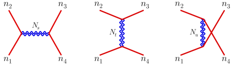
Figure 1: Feynman diagrams for the scattering of gravitational KK Goldstone bosons, $\phi_{n_{1}}\phi_{n_{2}}\!\!\!\rightarrow\!\phi_{n_{3}}\phi_{n_{4}}$, by exchanging the KK gravitons of level-$N_{j}$ ($\,j=s,t,u)$ at the tree level, which contribute the leading energy-dependence of $\mathcal{O}(E^{2})$.

For inelastic scattering of gravitational KK Goldstone bosons, we compute the four-point amplitudes and find that the LO inelastic amplitude is connected to the LO elastic amplitude (8) by the following relation:

$$\widetilde{\mathcal{M}}[\phi_{n_{1}}\phi_{n_{2}}\!\!\!\rightarrow\!\phi_{n_{3}}\phi_{n_{4}}]\,=\,\zeta\widetilde{\mathcal{M}}[\phi_{n}\phi_{n}\!\!\rightarrow\!\!\phi_{n}\phi_{n}]\hskip 0.85358pt,$$ (11)

where $\,\zeta\!=\!2/3\,$ for $\,n_{1}\!=\!n_{2}\!\neq\!n_{3}\!=\!n_{4}\,$,  and $\,\zeta\!=\!1/3\,$ for the cases with KK numbers $(n_{1},n_{2},$ $n_{3},n_{4})$ having no more than one equality.

Table 1: Kinematic numerators of the LO and NLO scattering amplitudes for KK longitudinal gauge bosons and KK Goldstones as defined in Eq.(12), where $(\mathcal{N}_{j},\,\widetilde{\mathcal{N}}_{j})=(\mathcal{N}_{j}^{0},\,\widetilde{\mathcal{N}}_{j}^{0})\!+\!(\delta\mathcal{N}_{j},\,\delta\widetilde{\mathcal{N}}_{j})=\mathcal{O}(E^{2}M_{n}^{0})+\mathcal{O}(E^{0}M_{n}^{2})$, and $(s_{\theta},\,c_{\theta})=(\sin\theta,\,\cos\theta)$.

Numerators	$\mathcal{N}_{s}$	$\mathcal{N}_{t}$	$\mathcal{N}_{u}$	$\quad\widetilde{\mathcal{N}}_{s}\quad$	$\widetilde{\mathcal{N}}_{t}$	$\widetilde{\mathcal{N}}_{u}$	$\,\mathcal{N}_{s}\!-\!\widetilde{\mathcal{N}}_{s}\,$	$\,\mathcal{N}_{t}\!-\!\widetilde{\mathcal{N}}_{t}\,$	$\,\mathcal{N}_{u}\!-\!\widetilde{\mathcal{N}}_{u}\,$
$\mathcal{N}^{0}_{j}/s_{j}$	$\frac{\,5c_{\theta}\,}{2}$	$\frac{\,13+5c_{\theta}+4c_{2\theta}\,}{2(1+c_{\theta})\,}$	$-\frac{\,13-5c_{\theta}+4c_{2\theta}\,}{2(1-c_{\theta})\,}$	$-\frac{\,3c_{\theta}\,}{2}$	$\frac{\,3(3-c_{\theta})\,}{2(1+c_{\theta})\,}$	$-\frac{\,3(3+c_{\theta})\,}{2(1-c_{\theta})\,}$	$4c_{\theta}$	$4c_{\theta}$	$4c_{\theta}$
$\delta\mathcal{N}_{j}/M_{n}^{2}$	$4c_{\theta}$	$\frac{\,2(2-3c_{\theta}-2c_{2\theta}-c_{3\theta})\,}{1+c_{\theta}\,}$	$-\frac{\,2(2+3c_{\theta}-2c_{2\theta}+c_{3\theta})\,}{1-c_{\theta}\,}$	$\,4c_{\theta}\,$	$-\frac{\,8c_{\theta}\,}{\,1+c_{\theta}\,}$	$-\frac{\,8c_{\theta}\,}{\,1-c_{\theta}\,}$	$0$	$8s_{\theta}^{2}$	$-8s_{\theta}^{2}$

V Double-Copy Construction of Massive
KK Scattering Amplitudes

The double-copy construction for the massive KK gauge/gravity scattering amplitudes are highly nontrivial. We make the first serious attempt for an explicit double-copy construction of KK amplitudes under high energy expansion. We present the four-point elastic scattering amplitudes of longitudinal KK gauge bosons (Goldstones) at the LO and NLO:

$$\mathcal{T} =\sum_{j}\!\frac{\,g^{2}\mathcal{C}_{j}\mathcal{N}_{j}}{s_{j}}=\sum_{j}\!\frac{\,g^{2}\mathcal{C}_{j}(\mathcal{N}^{0}_{j}\!+\delta\mathcal{N}_{j})}{s_{j}}=\mathcal{T}_{0}\!+\delta\mathcal{T},$$ (12a)

$$\widetilde{\mathcal{T}} =\sum_{j}\!\frac{\,g^{2}\mathcal{C}_{j}\widetilde{\mathcal{N}}_{j}}{s_{j}}=\sum_{j}\!\frac{\,g^{2}\mathcal{C}_{j}(\widetilde{\mathcal{N}}^{0}_{j}\!+\delta\widetilde{\mathcal{N}}_{j})}{s_{j}}=\widetilde{\mathcal{T}}_{0}\!+\delta\widetilde{\mathcal{T}},$$ (12b)

where we have denoted $\,\mathcal{T}\!\equiv\!\mathcal{T}[A^{an}_{L}A^{bn}_{L}\!\!\rightarrow\!\!A^{cn}_{L}A^{dn}_{L}]$ and $\widetilde{\mathcal{T}}\!\equiv\widetilde{\mathcal{T}}[A^{an}_{5}A^{bn}_{5}\!\!\rightarrow\!\!A^{cn}_{5}A^{dn}_{5}]$. We also define the SU($N$) color factors as $(\mathcal{C}_{s},\,\mathcal{C}_{t},\,\mathcal{C}_{u})\!\equiv\!\left(C^{abe}C^{cde}\!,\,C^{ade}C^{bce}\!,\,C^{ace}C^{dbe}\right)$, which obey the Jacobi identity $\,\mathcal{C}_{s}\!+\mathcal{C}_{t}\!+\mathcal{C}_{u}\!=0\hskip 0.85358pt$.

We present in Table 1 the numerator factors ($\mathcal{N}_{j},\,\widetilde{\mathcal{N}}_{j}$) of Eqs.(12a)-(12b). Table 1 shows that $(\mathcal{T}_{0},\,\widetilde{\mathcal{T}}_{0})\!\!=\mathcal{O}(E^{0}M_{n}^{0})$ and $(\delta\mathcal{T},\,\delta\widetilde{\mathcal{T}})=\mathcal{O}(M_{n}^{2}/E^{2})\hskip 0.85358pt$. We find that the sum of each set of the LO, NLO, and NNLO numerators of the KK gauge (Goldstone) scattering amplitudes in Eq.(12) violate the kinematic Jacobi identity by terms of $\mathcal{O}(M_{n}^{2})$ and $\mathcal{O}(M_{n}^{4}/E^{2})$, respectively:

$$\sum_{j}\!\mathcal{N}_{j}^{0}=10\hskip 0.85358ptc_{\theta}M_{n}^{2}\,,~{}~{}~{}~{}\sum_{j}\!\widetilde{\mathcal{N}}_{j}^{0}=-6\hskip 0.85358ptc_{\theta}M_{n}^{2}\,,$$ (13a)

$$\sum_{j}\!\delta_{1}\mathcal{N}_{j}=\sum_{j}\!\delta_{1}\widetilde{\mathcal{N}}_{j}=-2\hskip 0.85358pt(7+c_{2\theta})c_{\theta}\csc^{2}\!\theta\hskip 0.85358ptM_{n}^{2}\,,$$ (13b)

$$\sum_{j}\!\delta_{2}\mathcal{N}_{j}=8\hskip 0.85358pt(31+c_{4\theta})\hskip 0.85358ptc_{\theta}\csc^{4}\!\theta\hskip 0.85358ptM_{n}^{4}/s\,,$$ (13c)

$$\sum_{j}\!\delta_{2}\widetilde{\mathcal{N}}_{j}=32\hskip 0.85358pt(7+c_{2\theta})\hskip 0.85358ptc_{\theta}\csc^{4}\!\theta\hskip 0.85358ptM_{n}^{4}/s\,,$$ (13d)

where $\,c_{n\theta}\!=\cos(n\theta)\hskip 0.85358pt$, $\delta\mathcal{N}_{j}\!=\!\delta_{1}\mathcal{N}_{j}\!+\delta_{2}\mathcal{N}_{j}$, and $\,\delta\widetilde{\mathcal{N}}_{j}\!=$ $\delta_{1}\widetilde{\mathcal{N}}_{j}\!+\delta_{2}\widetilde{\mathcal{N}}_{j}\hskip 0.85358pt$. Hence, we cannot naively apply color-kinematics duality for BCJ-type double-copy construction without making further modifications on these numerators.

Inspecting the scattering amplitudes in Eq.(12), we first observe that they are invariant under the following generalized gauge transformations of their numerators:

$$\mathcal{N}_{j}^{\prime}=\mathcal{N}_{j}+s_{j}\hskip 0.85358pt\Delta\,,~{}~{}~{}~{}\widetilde{\mathcal{N}}_{j}^{\prime}=\widetilde{\mathcal{N}}_{j}+s_{j}\hskip 0.85358pt\widetilde{\Delta}\,.$$ (14)

We can determine the gauge-parameters $(\Delta,\,\widetilde{\Delta})$ by requiring the gauge-transformed numerators to obey the Jacobi identities $\sum_{j}\mathcal{N}_{j}^{\prime}\!=0\hskip 0.85358pt$ and $\sum_{j}\widetilde{\mathcal{N}}_{j}^{\prime}\!=0\,$. Thus, we derive the following general solutions:

$$\Delta=-\frac{1}{\,4M_{n}^{2}\,}\!\sum_{j}\mathcal{N}_{j}\,,~{}~{}~{}~{}\widetilde{\Delta}=-\frac{1}{\,4M_{n}^{2}\,}\!\sum_{j}\widetilde{\mathcal{N}}_{j}\,,~{}~{}~{}~{}~{}$$ (15)

which realize the BCJ-respecting numerators $(\mathcal{N}_{j}^{\prime},\,\widetilde{\mathcal{N}}_{j}^{\prime})$. Making high energy expansions on both sides of Eq. (15), we derive the expressions of the gauge-parameters $(\Delta,\,\widetilde{\Delta})=(\Delta_{0}+\Delta_{1},\,\widetilde{\Delta}_{0}+\widetilde{\Delta}_{1})\,$ at the LO and NLO :

$$\Delta_{0} =\mbox{$\frac{\,{1}\,}{4}$}(9+7\hskip 0.85358ptc_{2\theta})\hskip 0.85358ptc_{\theta}\csc^{2}\!\theta\,,~{}~{}~{}$$ (16)

$$\widetilde{\Delta}_{0} =\mbox{$\frac{\,{1}\,}{4}$}(17\!-c_{2\theta})\hskip 0.85358ptc_{\theta}\csc^{2}\!\theta\,,$$

$$\Delta_{1} =-2(31+c_{4\theta})c_{\theta}\csc^{4}\!\theta\,(M_{n}^{2}/s)\,,\qquad$$

$$\widetilde{\Delta}_{1} =-8(7+c_{2\theta})c_{\theta}\csc^{4}\!\theta\,(M_{n}^{2}/s)\,.$$

With these, we further compute the new numerators $(\mathcal{N}_{j}^{\prime},\,\widetilde{\mathcal{N}}_{j}^{\prime})$, and derive explicitly the LO results in Eq.(19) and the NLO results in the Supplemental Material supp .

For the 5d KK YM (YM5) and 5d KK GR (GR5) theories, we expect the double-copy correspondence between the KK gauge fields and KK graviton fields:

$$A_{n}^{a\mu}\!\otimes\!A_{n}^{a\nu} \longrightarrow ~{}h^{\mu\nu}_{n}\,,$$

$$A_{n}^{a5}\!\otimes\!A_{n}^{a5} \longrightarrow ~{}h^{55}_{n}\,,$$ (17)

$$A_{n}^{a\mu}\!\otimes\!A_{n}^{a5} \longrightarrow ~{}h^{\mu 5}_{n}\,.$$

The physical spin-2 KK graviton field $h^{\mu\nu}_{n}$ arises from two copies of spin-1 KK gauge fields. The KK Goldstone boson $A_{n}^{a5}$ of the YM5 has its double-copy counterparts $h^{55}_{n}\,(=\!\!\phi_{n})$ and $h^{\mu 5}_{n}\,(=\!\!\mathcal{A}^{\mu}_{n})$ which correspond to the scalar and vector KK Goldstone bosons in the compactified GR5 theory. The double-copy correspondence between the longitudinal KK modes, $A_{L}^{an}\!\!\otimes\!A_{L}^{an}\!\!\rightarrow\!\!h_{L}^{n}$,  is highly nontrivial even at the LO of high energy expansion, because $(A_{L}^{an},\hskip 0.85358pth_{L}^{n})$ do not exist in $M_{n}\!\!\rightarrow\!0$ limit and the KK Goldstone bosons $(A_{5}^{an},\hskip 0.85358pt\phi_{n})$ become physical states in massless limit. Hence, this double-copy is consistently realized only because we can use the KK GRET (GAET) to connect $h_{L}^{n}\,(A_{L}^{an}$) amplitudes to the $\phi_{n}\,(A_{5}^{an}$) amplitudes under the $M_{n}/E\!\rightarrow\!\hskip 0.85358pt0$  limit where we can hold the KK mass $M_{n}$ fixed and take the energy $\hskip 0.85358ptE\!\rightarrow\!\infty\hskip 0.85358pt$.

Then, we extend the conventional double-copy method BCJ:2008 BCJ:2019 to the massive KK YM theory under high energy expansion. We apply the correspondence of color-kinematics duality $\,\mathcal{C}_{j}\!\!\rightarrow\!\mathcal{N}^{\prime}_{j}\,$ to Eq.(12a) and $\,\mathcal{C}_{j}\!\!\rightarrow\!\widetilde{\mathcal{N}}^{\prime}_{j}$ to Eq.(12b). Thus, we can construct the following four-particle KK graviton (Goldstone) amplitudes:

$$\mathcal{M} \hskip 0.85358pt=\hskip 0.85358pt\sum_{j}\!\frac{~{}c_{0}\hskip 0.85358ptg^{2}(\mathcal{N}^{0\hskip 0.85358pt\prime}_{j}\!+\delta\mathcal{N}_{j}^{\prime})^{2}\,}{s_{j}}=\,\mathcal{M}_{0}\!+\delta\mathcal{M}\,,$$ (18a)

$$\widetilde{\mathcal{M}} \hskip 0.85358pt=\hskip 0.85358pt\sum_{j}\!\frac{~{}c_{0}\hskip 0.85358ptg^{2}(\widetilde{\mathcal{N}}^{0\hskip 0.85358pt\prime}_{j}\!+\delta\widetilde{\mathcal{N}}_{j}^{\prime})^{2}\,}{s_{j}}=\hskip 0.85358pt\widetilde{\mathcal{M}}_{0}+\delta\widetilde{\mathcal{M}}\,,$$ (18b)

where we have denoted the scattering amplitudes $\mathcal{M}\!\equiv\!\mathcal{M}[h_{L}^{n}h_{L}^{n}\!\!\rightarrow\!\!h_{L}^{n}h_{L}^{n}]$ and $\widetilde{\mathcal{M}}\!\equiv\!\widetilde{\mathcal{M}}[\phi_{n}\phi_{n}\!\!\rightarrow\!\phi_{n}\phi_{n}]$, and $c_{0}$ is a conversion constant.

From Table 1 and using Eqs.(14)(16), we find that the LO numerators $(\mathcal{N}_{j}^{0\hskip 0.85358pt\prime},\,\widetilde{\mathcal{N}}_{j}^{0\hskip 0.85358pt\prime})$ are mass-independent and equal to each other :

$$\mathcal{N}_{s}^{0\hskip 0.85358pt\prime} \!=\widetilde{\mathcal{N}}_{s}^{0\hskip 0.85358pt\prime}\!=\frac{~{}s\hskip 0.85358pt(7\!+\!c_{2\theta})c_{\theta}~{}}{2\sin^{2}\!\theta}\hskip 0.85358pt,$$ (19a)

$$\mathcal{N}_{t}^{0\hskip 0.85358pt\prime} \!=\widetilde{\mathcal{N}}_{t}^{0\hskip 0.85358pt\prime}\!=-\frac{~{}s\hskip 0.85358pt(42\!-\!15c_{\theta}\!+\!6c_{2\theta}\!-\!c_{3\theta})~{}}{16\hskip 0.85358pt(1\!-\!c_{\theta})}\hskip 0.85358pt,\hskip 14.22636pt$$ (19b)

$$\mathcal{N}_{u}^{0\hskip 0.85358pt\prime} \!=\widetilde{\mathcal{N}}_{u}^{0\hskip 0.85358pt\prime}\!=\frac{~{}s\hskip 0.85358pt(42\!+\!15c_{\theta}\!+\!6c_{2\theta}\!+\!c_{3\theta})~{}}{16\hskip 0.85358pt(1\!+\!c_{\theta})}\hskip 0.85358pt.$$ (19c)

This demonstrates the equivalence between the two leading-order KK amplitudes at $\mathcal{O}(E^{0}M_{n}^{0})$, $\,\mathcal{T}_{0}=\widetilde{\mathcal{T}}_{0}\,$, which explicitly realizes the KK GAET. With these and using our LO double-copy formulas in Eq.(18), we can reconstruct the KK GRET:

$$\mathcal{M}_{0}[\mathrm{DC}]\,=\,\widetilde{\mathcal{M}}_{0}[\mathrm{DC}]\,,$$ (20)

which is of $\,\mathcal{O}(E^{2}M_{n}^{0})\hskip 0.85358pt$. We stress that as expected, these LO amplitudes are mass-independent and thus the LO double-copy can hold universally.  We further find that after setting the overall conversion constant of Eq.(18) as $\,c_{0}\!=\!-\kappa^{2}/(24g^{2})\hskip 0.85358pt$,  the reconstructed LO KK amplitude $\,\mathcal{M}_{0}\,(\widetilde{\mathcal{M}}_{0})\,$ just equals the LO KK Goldstone amplitude (8) and the corresponding LO longitudinal KK graviton amplitude supp . Hence, our double-copy prediction (20) can prove (reconstruct) the KK GRET $\,\mathcal{M}_{0}\!=\!\widetilde{\mathcal{M}}_{0}$  from the KK GAET $\,\mathcal{T}_{0}=\widetilde{\mathcal{T}}_{0}\,$. We derived this GRET relation in Eq.(9) by direct Feynman-diagram calculations. Note that the KK GAET relation $\,\mathcal{T}_{0}=\widetilde{\mathcal{T}}_{0}\,$ can hold for general $N$-point longitudinal KK gauge (Goldstone) amplitudes 5DYM2002 KK-ET-He2004 . Hence, making double-copy on both sides of $\,\mathcal{T}_{0}\!=\!\widetilde{\mathcal{T}}_{0}\,$ can establish the GRET (20) to hold for $N$-point longitudinal KK graviton (Goldstone) amplitudes. From this, we can further establish a new correspondence between the two types of energy cancellations in the $N$-longitudinal KK gauge boson amplitudes and in the corresponding $N$-longitudinal KK graviton amplitudes (cf. the discussion around the end of Sec. III).

Next, we use the double-copy formulas (18a)-(18b) to reconstruct the four-point longitudinal KK graviton amplitude and the corresponding KK Goldstone boson amplitude at the NLO:

$$\frac{\delta\mathcal{M}(\mathrm{DC})\,}{\kappa^{2}M_{n}^{2}} =-\frac{\,5(1642+297\hskip 0.85358ptc_{2\theta}+102\hskip 0.85358ptc_{4\theta}+7\hskip 0.85358ptc_{6\theta})\,}{768\sin^{4}\theta}\hskip 0.85358pt,$$ (21a)

$$\frac{\delta\widetilde{\mathcal{M}}(\mathrm{DC})}{\kappa^{2}M_{n}^{2}} =-\frac{\,6386+3837\hskip 0.85358ptc_{2\theta}+30\hskip 0.85358ptc_{4\theta}-13\hskip 0.85358ptc_{6\theta}\,}{768\sin^{4}\theta}\hskip 0.85358pt.$$ (21b)

They have the same size of $\mathcal{O}(\kappa^{2}M_{n}^{2})$ and the same angular structure of $\hskip 0.85358pt(1,\,c_{2\theta},\,c_{4\theta},\,c_{6\theta})\!\times\csc^{4}\theta\,$ as the original NLO amplitudes $(\delta\mathcal{M},\,\delta\widetilde{\mathcal{M}})$ derived from Feynman diagram calculations supp , though their numerical coefficients still differ. Then, using Eq.(21) we compute the difference between the two double-copied NLO amplitudes $\,\Delta\mathcal{M}(\mathrm{DC})\!\!=\!\delta\mathcal{M}\!-\!\delta\widetilde{\mathcal{M}}\,$ and compare it with the NLO amplitude-difference $\Delta\mathcal{M}(\mathrm{GR5})$ by Feynman diagram calculations in the KK GR5 theory:

$$\Delta\mathcal{M}(\mathrm{GR5}) =-\mbox{$\frac{\,{3}\,}{2}$}\kappa^{2}\!M_{n}^{2}\left(19.5+c_{2\theta}\right),$$ (22a)

$$\Delta\mathcal{M}(\mathrm{DC}) =-\kappa^{2}M_{n}^{2}\,(7\!+c_{2\theta})\,.$$ (22b)

We find that they also have the same size of $\mathcal{O}(\kappa^{2}M_{n}^{2})$ and the same angular structure of $\hskip 0.85358pt(1,\,c_{2\theta})\hskip 0.85358pt$. Eq.(22a) shows that the difference $\Delta\mathcal{M}(\text{GR5})$ between the original NLO amplitudes exhibits a striking precise cancellations of the angular structure $\hskip 0.85358pt(1,\,c_{2\theta},\,c_{4\theta},\,c_{6\theta})\!\times\csc^{4}\theta\,$ to $\hskip 0.85358pt(1,\,c_{2\theta})\hskip 0.85358pt$. Impressively, our double-copied NLO amplitude-difference $\Delta\mathcal{M}(\text{DC})$ in Eq.(22b) can also realize the same type of the precise angular cancellations.

The above extended NLO double-copy results (21) and (22b) are truly encouraging, because they already give the correct structure of the NLO KK amplitudes including the precise cancellations of the angular dependence in Eqs.(21)-(22). These strongly suggest that our massive KK double-copy approach is on the right track. Its importance is twofold: (i). In practice, for our proposed KK double-copy method under high energy expansion, the LO double-copy construction is the most important part because it newly establishes the GRET relation $\mathcal{M}_{0}\!=\!\widetilde{\mathcal{M}}_{0}$ [Eq. (20)] from the GAET relation $\,\mathcal{T}_{0}\!=\!\widetilde{\mathcal{T}}_{0}\,$ [Eq.(19) and below], as will be shown in Eq.(34). The NLO KK graviton amplitudes are relevant only when we estimate the size of the residual term $\mathcal{M}_{\!\Delta}$ of our GRET (7) and here we do not need the precise form of $\mathcal{M}_{\!\Delta}$ except to justify its size $\mathcal{M}_{\!\Delta}\!\!=\mathcal{O}(E^{0}M_{n}^{2})$ by the double-copy construction [cf. Eq.(33)]. This proves that the residual term $\mathcal{M}_{\!\Delta}\!$ does belong to the NLO amplitudes and is neligible for our GRET formulation in the high energy limit. Hence, we do not need any precise NLO double-copy here. (ii). In general, our current KK double-copy approach as the first serious attempt to construct the massive KK graviton amplitudes has given strong motivation and important guideline for a full resolution of the exact double-copy beyond the LO. Our further study has found out the reasons for the minor mismatch between the numerical coefficients of the double-copied NLO amplitudes (21) and that of the direct Feynman-diagram calculations. One reason is due to the double-pole structure in the KK amplitudes (including exchanges of both the zero-mode and KK-modes) beyond the conventional massless theories, so the additional KK mass-poles contribute to our mass-dependent NLO amplitudes and cause a mismatch. Another reason is because the exact polarization tensor of the (helicity-zero) longitudinal KK graviton is given by $\,\varepsilon_{L}^{\mu\nu}\!=\!\left(\epsilon_{+}^{\mu}\epsilon_{-}^{\nu}\!+\epsilon_{-}^{\mu}\epsilon_{+}^{\nu}\!+2\epsilon_{L}^{\mu}\epsilon_{L}^{\nu}\right)/\sqrt{6\,}$ supp , which constains not only the longitudinal product $\epsilon_{L}^{\mu}\epsilon_{L}^{\nu}$, but also the transverse products $\,\epsilon_{+}^{\mu}\epsilon_{-}^{\nu}\!+\epsilon_{-}^{\mu}\epsilon_{+}^{\nu}\hskip 0.85358pt$. Thus, the other scattering amplitudes containing possible transversely polarized external KK gauge boson states should be included for a full double-copy besides the four-longitudinal KK gauge boson amplitude in Eq.(12).

With these in minds, we have further used a first principle approach of the KK string theory in our recent work Li:2021yfk to derive the extended massive KLT-like relations between the product of the KK open string amplitudes and the KK closed string amplitude. In the field theory limit, we can derive the exact double-copy relations between the product of the KK gauge boson amplitudes and the KK graviton amplitude at tree level Li:2021yfk . In such exact double-copy relations all the relevant helicity indices of the external KK gauge boson states are summed over to match the corresponding polarization tensors of the external KK graviton states. The double-pole structure is also avoided by first making the 5d compactification under $S^{1}$ (without orbifold) where the KK numbers ($\pm n\!=\!\pm 1,\pm 2,\pm 3,\cdots$) are strictly conserved and the amplitudes are ensured to have single-pole structure. Then, we can define the $\mathbb{Z}_{2}$-even (odd) KK states as $\,|n_{\pm}\rangle=(|+n\rangle\pm|-n\rangle)/\!\sqrt{2\,}$, and derive the amplitudes under $S^{1}\!/\mathbb{Z}_{2}$ compactification from the combinations of those amplitudes under the $S^{1}$ compactification Li:2021yfk . Using this improved massive double-copy approach, we can exactly reconstruct all the massive KK graviton amplitudes at tree level. For the four longitudinal KK graviton amplitudes under $S^{1}\!/\mathbb{Z}_{2}$, we derive the following (BCJ-type) exact massive double-copy formula:

$$\mathcal{M}=-\frac{\kappa^{2}}{64}\sum_{\mathsf{P}}\!\sum_{j}\!\sum_{\lambda_{k},\lambda^{\prime}_{k}}\!\prod_{k}C_{\lambda_{k}\lambda^{\prime}_{k}}\frac{\,N_{j}^{\mathsf{P}}(\lambda_{k})N_{j}^{\mathsf{P}}(\lambda_{k}^{\prime})\,}{D_{j}}\,,$$ (23)

where $\{N_{j}\}$ denote the kinematic numerators under the $S^{1}$ compactification and each external KK gauge boson has 3 helicity states (with $\lambda_{k}\!=\!\pm 1,L$ and $k\!=\!1,2,3,4$). We use $\mathsf{P}\!=\!\{n_{1},n_{2},n_{3},n_{4}\}$ to label each possible combination of the KK numbers for external gauge bosons, which obey the condition of KK number conservation $\sum_{k=1}^{4}\!n_{k}\!=\!0$ . For the elastic KK scattering, we have

$$\mathsf{P}= \ \{\pm n,\pm n,\mp n,\mp n\},\hskip 5.69054pt\{\pm n,\mp n,\pm n,\mp n\},~{}~{}~{}$$ (24)

$$\ \{\pm n,\mp n,\mp n,\pm n\}.$$

In Eq.(23), $C_{\lambda_{k}\lambda^{\prime}_{k}}$ denotes the coefficients in the longitudinal polarization tensor of $k$-th external KK graviton supp , $\varepsilon_{L,k}^{\mu\nu}\!=\!\sum C_{\lambda_{k}\lambda^{\prime}_{k}}\epsilon_{\lambda_{k}}^{\mu}\epsilon_{\lambda^{\prime}_{k}}^{\nu}$, where $\lambda_{k},\lambda^{\prime}_{k}\!=\!\pm 1,L$ are the helicity indices for the $k$-th external gauge boson. The denominator of Eq.(23) is defined as $D_{j}\!=\!s_{j}\!-\!M_{j}^{2}$, where $\,s_{j}\!\in\!\{s,t,u\}\,$ and $M_{j}^{2}\!\in\!\{M_{n_{1}+n_{2}}^{2},M_{n_{1}+n_{4}}^{2},M_{n_{1}+n_{3}}^{2}\}$.

Then, we make high energy expansion for the corresponding elastic amplitude of KK gauge bosons (under $S^{1}$ compactification) at the LO and NLO:

$$\mathcal{T} \,=\,g^{2}\sum_{j}\frac{\,\mathcal{C}_{j}N_{j}^{\mathsf{P}}}{D_{j}}=g^{2}\sum_{j}\!\frac{\,\mathcal{C}_{j}(N^{0,\mathsf{P}}_{j}\!+\delta N^{\mathsf{P}}_{j})}{s_{j}}\hskip 19.91692pt$$

$$\,=~{}\mathcal{T}_{0}+\delta\mathcal{T}\,,$$ (25a)

$$N_{j}^{\mathsf{P}} \,=~{}\frac{\,D_{j}\,}{s_{j}}\!\left(\!{N_{j}^{0,\mathsf{P}}}+\delta N^{\mathsf{P}}_{j}\right)\!.$$ (25b)

With this, we expand the exact double-copy formula of the longitudinal KK graviton amplitude (23) under the high energy expansion of $1/s$ :

$$\mathcal{M} =-\frac{~{}\kappa^{2}\,}{64}\,\sum_{\mathsf{P}}\sum_{j}\!\sum_{\lambda_{k},\lambda^{\prime}_{k}}\prod_{k}C_{\lambda_{k}\lambda^{\prime}_{k}}\frac{\,D_{j}\,}{s_{j}^{2}}$$

$$\hskip 14.22636pt\times\!\left[\,\!N_{j}^{0,\mathsf{P}}(\lambda_{k})\!+\delta N_{j}^{\mathsf{P}}(\lambda_{k})\!\,\right]\!\left[\,\!N_{j}^{0,\mathsf{P}}(\lambda^{\prime}_{k})\!+\delta N_{j}^{\mathsf{P}}(\lambda^{\prime}_{k})\!\,\right]\hskip 11.38109pt$$

$$=\,\mathcal{M}_{0}+\delta\mathcal{M}\,.$$ (26)

It can be proven that the above double-copied LO amplitude $\mathcal{M}_{0}$ is equivalent to the LO amplitude given in Eq.(18a) Li:2021yfk . We explicitly compute the above LO amplitude $\mathcal{M}_{0}$ and find that $\mathcal{M}_{0}$ just equals that of Eq.(8) as well as Eq.(S22a) supp . Then, we further compute the above double-copied NLO amplitude $\delta\mathcal{M}$ as follows:

$$\delta\mathcal{M}=-\frac{\kappa^{2}M_{n}^{2}}{256}(1810+93\hskip 0.85358ptc_{2\theta}+126\hskip 0.85358ptc_{4\theta}+19\hskip 0.85358ptc_{6\theta})\csc^{4}\theta\hskip 0.85358pt.$$ (27)

We find that this fully agrees with the exact NLO elastic KK graviton amplitude derived from the direct Feynman diagram calculation in Eq.(S22b) of the supplemental material supp . The above analysis is an explicit demonstration that we can realize the exact (BCJ-type) massive double-copy construction of the four-point KK graviton amplitudes in Eq.(23), as well as the precise double-copy of the KK graviton amplitudes (V)-(27) at both the LO and NLO of the high energy expansion. We will systematically pursue this new direction in our future work.

Finally, it is very impressive that our improved massive double-copy construction of the longitudinal KK graviton (KK Goldstone) amplitude in Eq.(18) is based on the pure longitudinal KK gauge (KK Goldstone) amplitude (12) alone, which can already give not only the precise LO KK graviton (KK Goldstone) amplitude, but also the correct structure of the NLO KK graviton (KK Goldstone) amplitude (21). In the following, we will propose another improved double-copy method to further reproduce the exact longitudinal KK graviton (KK Goldstone) amplitudes at the NLO and beyond. It only uses the amplitudes of pure longitudinal KK gauge bosons (KK Goldstone bosons) alone, hence it is practically simple and valuable. For this, we construct the following improved NLO numerators:

$$(\delta\mathcal{N}_{s}^{\prime\prime},\,\delta\mathcal{N}_{t}^{\prime\prime},\,\delta\mathcal{N}_{u}^{\prime\prime}) =(\delta\mathcal{N}_{s}^{\prime},\,\delta\mathcal{N}_{t}^{\prime}\!-\!z,\,\delta\mathcal{N}_{u}^{\prime}\!+\!z\,)\hskip 0.85358pt,$$ (28a)

$$(\delta\widetilde{\mathcal{N}}_{s}^{\prime\prime},\,\delta\widetilde{\mathcal{N}}_{t}^{\prime\prime},\,\delta\widetilde{\mathcal{N}}_{u}^{\prime\prime}) =(\delta\widetilde{\mathcal{N}}_{s}^{\prime},\,\delta\widetilde{\mathcal{N}}_{t}^{\prime}\!-\!\tilde{z},\,\delta\widetilde{\mathcal{N}}_{u}^{\prime}\!+\!\tilde{z}\,)\hskip 0.85358pt,$$ (28b)

where $(z,\,\tilde{z})$ are functions of $\,\theta\,$ and can be determined by matching our improved NLO KK amplitudes of double-copy with the original NLO KK graviton (Goldstone) amplitudes of the GR5. Then, we solve $(z,\,\tilde{z})$ as

$$z \,=\,\frac{\,M_{n}^{2}(1390\!+\!603c_{2\theta}\!+\!66c_{4\theta}\!-11c_{6\theta})\,}{12\hskip 0.85358pt(13\!-\!12c_{2\theta}\!-\!c_{4\theta})}\,,$$ (29a)

$$\tilde{z} \,=\,\frac{\,M_{n}^{2}(4546\!-\!3585c_{2\theta}\!+\!1086c_{4\theta}\!+c_{6\theta})\,}{12\left(13\!-\!12c_{2\theta}\!-\!c_{4\theta}\right)}\,.$$ (29b)

Note that the modified kinematic numerators (28) continue to hold the Jacobi identity. Because the corresponding NLO gauge (Goldstone) amplitudes $(\delta\mathcal{T}^{\prime\prime},\,\delta\widetilde{\mathcal{T}}^{\prime\prime})$ are modified only by terms of NLO, so we can still hold the general GAET identity $\hskip 0.85358pt\mathcal{T}^{\prime\prime}\!=\widetilde{\mathcal{T}}^{\prime\prime}\!+\mathcal{T}_{v}^{\prime\prime}\hskip 0.85358pt$ by redefining the residual term as $\,\mathcal{T}_{v}^{\prime\prime}\!=\mathcal{T}_{v}\!-g^{2}(\mathcal{C}_{t}/t\!-\mathcal{C}_{u}/u)(z\!-\!\tilde{z})\hskip 0.85358pt$. Using Eqs.(28)-(29), we can reproduce the exact NLO KK gravitational scattering amplitudes [shown in Eqs.(S22a)-(S22b) of the Supplemental Material supp ]. This double-copy procedure can be further applied to higher orders beyond the NLO when needed.

VI GRET Residual Terms and Energy Cancellation

According to Table 1 and the generalized gauge transformation (14), we can explicitly deduce the equivalence between the KK gauge boson amplitude and the corresponding KK Goldstone boson amplitude:

$$\mathcal{T}_{0}\,=\,\widetilde{\mathcal{T}}_{0}\,,$$ (30)

which belongs to the LO of $\mathcal{O}(E^{0}M_{n}^{0})$. Using our double-copy method, we further derived the GRET relation $\mathcal{M}_{0}\!=\!\widetilde{\mathcal{M}}_{0}$ at the $\hskip 0.85358pt\mathcal{O}(E^{2}M_{n}^{0})\hskip 0.85358pt$ as shown in Eq. (20). Thus, the residual terms of the GAET and the GRET (7) are given by the differences between the KK longitudinal amplitude and KK Goldstone amplitude at the NLO :

$$\mathcal{T}_{v} \equiv\sum\!\mathcal{T}[A_{5}^{n},v_{n}]=\delta\mathcal{T}\!-\!\delta\widetilde{\mathcal{T}}\,=\,\mathcal{O}(M_{n}^{2}/E^{2})\,,$$ (31a)

$$\mathcal{M}_{\Delta} \equiv\sum\!\mathcal{M}[\widetilde{\Delta}_{n},\phi_{n}]=\delta\mathcal{M}\!-\!\delta\widetilde{\mathcal{M}}=\mathcal{O}(E^{0}M_{n}^{2})\,.$$ (31b)

The size of $\,\mathcal{T}_{v}=\mathcal{O}(M_{n}^{2}/E^{2})\,$ can be easily understood by using our generalized power counting rule supp . But, making the direct power counting gives $\,\mathcal{M}_{\Delta}\!=\mathcal{O}(E^{2})\,$ for its individual amplitudes, which has the same energy dependence as the LO KK Goldstone amplitude (8).

We can further determine the size of the residual term $\,\mathcal{M}_{\Delta}$  by the double-copy construction (18) based upon the KK gauge (Goldstone) boson scattering amplitudes of the YM5 theory alone (which are well understood 5DYM2002 5DYM2002-2 KK-ET-He2004 5dSM ). From Eq.(18) and Table 1, we can estimate the residual term by power counting:

$$\mathcal{M}_{\Delta} =\,\mathcal{O}(\delta\mathcal{M},\hskip 0.85358pt\delta\widetilde{\mathcal{M}})=\mathcal{O}\!\left(\!\frac{\mathcal{N}_{j}^{0\hskip 0.85358pt\prime}\delta\mathcal{N}_{j}^{\prime}}{s_{j}},\,\frac{\widetilde{\mathcal{N}}_{j}^{0\hskip 0.85358pt\prime}\delta\widetilde{\mathcal{N}}_{j}^{\prime}}{s_{j}}\!\right)$$

$$=\,\mathcal{O}(E^{0}M_{n}^{2})\hskip 0.85358pt.$$ (32)

Thus, we deduce the double-copy correspondence between the residual term $\hskip 0.85358pt\mathcal{T}_{v}\hskip 0.85358pt$ of the GAET and the residual term $\mathcal{M}_{\Delta}$ of the GRET:

$$\mathcal{T}_{v}~{}\longrightarrow~{}\mathcal{M}_{\Delta}(\mathrm{DC})=\mathcal{O}(E^{0}M_{n}^{2})\hskip 0.85358pt.$$ (33)

Hence, our double-copy construction proves that the GRET residual term $\,\mathcal{M}_{\Delta}$  should have an energy cancellation $\,\mathcal{O}(E^{2})\!\rightarrow\!\mathcal{O}(E^{0})\,$ among its individual amplitudes in Eq.(7b). This proves that $\mathcal{M}_{\Delta}$ is much smaller than the leading KK Goldstone amplitude $\,\widetilde{\mathcal{M}}_{0}=\mathcal{O}(E^{2}M_{n}^{0})$  under the high energy expansion.

From the above double-copy construction, we can establish a new correspondence from the GAET of the KK YM5 theory to the GRET of the 5d KK GR (GR5):

$$\mathrm{GAET\,(YM5)}\ \Longrightarrow\ \mathrm{GRET\,(GR5)}\,.$$ (34)

We will give a systematically expanded analysis in the companison long paper Hang:2021fmp , which includes our elaborations of the current key points and our extension of KLT relations KLT (along with CHY CHY ) to the double-copy construction of massive KK graviton amplitudes.

VII Conclusions

In this work, we newly formulated the geometric “Higgs” mechanism for the mass generation of Kaluza-Klein (KK) gravitons of the compactified 5d GR (GR5) theory at both the Lagrangian level and the scattering $S$-matrix level. Using a general $R_{\xi}$ gauge-fixing of quantization, we proved that the KK graviton propagator is free from the longstanding problem of the vDVZ discontinuity vDVZ in the conventional Fierz-Pauli massive gravity PF Hinterbichler:2012 and demonstrated that the KK gravity theory can consistently realize the mass-generation for spin-2 KK gravitons.

We newly proposed and proved a Gravitational Equivalence Theorem (GRET) which connects the $N$-point scattering amplitudes of the longitudinal KK gravitons to that of the gravitational KK Goldstone bosons. We computed the four-point scattering amplitudes of KK Goldstone bosons in comparison with the longitudinal KK graviton amplitudes, and explicitly proved the equivalence between the leading amplitudes of the longitudinal KK graviton scattering and the corresponding KK Goldstone boson scattering at $\mathcal{O}(E^{2}M_{n}^{0})$.

We developed a generalized power counting method for massive KK gauge and gravity theories. Using the GRET and the new power counting rules, we established a general energy-cancellation mechanism under which the leading energy dependence of $N$-particle longitudinal KK graviton amplitudes ($\propto\!E^{2(N+1+L)}$) must cancel down to a much lower energy power ($\propto\!E^{2(1+L)}$) by an energy factor of $E^{2N}$, where $L$ denotes the loop number of the relevant Feynman diagram. For the case of longitudinal KK graviton scattering amplitudes with $N\!=\!4$ and $L\!=\!0$ , this proves the energy cancellations of $\,E^{10}\!\!\rightarrow\!E^{2}\hskip 0.85358pt$.

Extending the conventional massless double-copy method BCJ:2008 BCJ:2019 to the compactified massive KK YM and KK GR theories, we derived the Jacobi-respecting numerators and constructed the scattering amplitudes of longitudinal KK gravitons (KK Goldstone bosons) under high energy expansion. Using our extended massive double-copy approach, we constructed exact double-copy of the KK graviton scattering amplitudes at both the leading order (LO) and the next-to-leading order (NLO). Applying this massive double-copy method, we established a new correspondence between the two energy cancellations in the four-point longitudinal KK amplitudes: $E^{4}\!\!\rightarrow\!E^{0}\,$ in the 5d KK YM gauge theory and $\,E^{10}\!\!\rightarrow\!E^{2}\,$ in the 5d KK GR theory, which is connected to the double-copy correspondence between the GAET and GRET as we derived in Eq.(34). Furthermore, we analyzed the structure of the residual term $\,\mathcal{M}_{\!\Delta}$ in the GRET (7) and further uncovered a new energy-cancellation mechanism of $\,E^{2}\!\rightarrow\!E^{0}\,$ for the residual term of the GRET.

Finally, we stress that the geometric Higgs mechanism is a general consequence of the KK compactification of extra spatial dimensions and should be realized for other KK gravity theories with more than one extra dimensions or with nonflat extra dimensions. We note that our identity (6) results from the underlying gravitational diffeomorphism invariance and thus should generally hold for any compactified 5d KK GR theory with proper gauge-fixing functions. Thus, we expect that the GRET should generally hold for other 5d KK GR theories and take similar form as the present Eq.(7) GET-2 . For instance, we find that the geometric Higgs mechanism and the large energy-cancellations of the longitudinal KK graviton amplitudes are also realized in the compactified warped 5d space of the Randall-Sundrum model RS and our GRET will work in the similar way. Following the current work, it is encouraging to further study these interesting issues in our future work GET-2 . In passing, we recently proposed Hang:2021oso a brand-new topological equivalence theorem (TET) to formulate the topological mass-generation in the 3d topologically massive Yang-Mills theory (TMYM), with which we uncover the nontrivial energy cancellations in the $N$-point Chern-Simons scattering amplitudes of the massive physical gauge bosons, $E^{4}\!\rightarrow\!E^{4-N}$. We then made an extended double-copy construction of the four-point massive graviton scattering amplitude in the 3d topologically massive gravity (TMG) TMG and further proved Hang:2021oso the striking energy cancellations of $\hskip 0.85358ptE^{12}\!\rightarrow\!E^{1}\hskip 0.85358pt$ in such massive graviton scattering amplitude of the TMG theory.

Acknowledgements
This research was supported in part by the National Natural Science Foundation of China (under grants Nos. 11835005 and 11675086), and by the National Key R & D Program of China (under grant No. 2017YFA 0402204).

Supplementary Materials
In the following Supplementary Materials, we provide the relevant technical details for the analyses presented in the main text of this paper. I. Kinematics of KK scattering; II. Feynman rules for 5d KK GR theory; III. Power counting and energy cancellations for KK graviton amplitudes; IV. KK graviton and Goldstone scattering amplitudes.

This Supplemental Material provides in detail the relevant formulas, Feynman rules, and the KK power counter method for the analyses of the KK scattering amplitudes in the compactified 5d Yang-Mills (YM5) theory and the compactified 5d General Relativity (GR5) theory.

I Kinematics of KK Scattering

We consider $\,2\!\rightarrow\!2\,$ KK scattering process, with the four-momentum of each external state obeying the on-shell condition $\,p^{2}_{j}\!=\!-M_{j}^{2}$, ($j=1,2,3,4$). We number the external lines clockwise, with their momenta being out-going. Thus, the energy-momentum conservation gives $\,\sum_{j}p_{j}\!=0\,$, and the physical momenta of the two incident particles equal $-p_{1}$ and $-p_{2}$, respectively. For illustration, we take the elastic scattering $\,X_{n}X_{n}\!\!\rightarrow\!X_{n}X_{n}$ ($n\!\geqslant\!0$) as an example, where $X_{n}$ denotes any given KK state of level-$n$ and has $M_{j}\!=\!M_{n}$. For the KK theory, the external particle has mass $M_{n}$ for a given KK-state of level-$n$. Thus, in the center-of-mass frame, we define the momenta as follows:

$$p_{1}^{\mu} =-E\left(1,0,0,\beta\right)\,, \hskip 28.45274ptp_{2}^{\mu}=-E\left(1,0,0,-\beta\right)\,,$$ (S1)

$$p_{3}^{\mu} =E\left(1,\beta s_{\theta},0,\beta c_{\theta}\right)\,, \hskip 28.45274ptp_{4}^{\mu}=E\left(1,-\beta s_{\theta},0,-\beta c_{\theta}\right)\,,$$

where $(s_{\theta},\hskip 0.85358ptc_{\theta})=(\sin\theta,\,\cos\theta)$ and $\hskip 0.85358pt\beta\!=\!(1\!-\!M_{n}^{2}/E^{2})^{1/2}\hskip 0.85358pt$. With the above, we can define the following three Mandelstam variables:

$$s=-\left(p_{1}\!+p_{2}\right)^{2}\!=4E^{2},~{}~{}~{}~{}t=-\left(p_{1}\!+p_{4}\right)^{2}\!=-\mbox{$\frac{\,{1}\,}{2}$}s\hskip 0.85358pt\beta^{2}(1\!+\!c_{\theta})\hskip 0.85358pt,~{}~{}~{}~{}u=-\left(p_{1}\!+p_{3}\right)^{2}\!=-\mbox{$\frac{\,{1}\,}{2}$}s\hskip 0.85358pt\beta^{2}(1\!-\!c_{\theta})\hskip 0.85358pt.$$ (S2)

Then, using the on-shell condition $E^{2}\!=E^{2}\beta^{2}+M_{n}^{2}\hskip 0.85358pt$, we define a new set of mass-independent Mandelstam variables as follows:

$$s_{0}=4E^{2}\beta^{2},\qquad t_{0}=-\frac{\,s_{0}\,}{2}(1+c_{\theta})\hskip 0.85358pt,\qquad u_{0}=-\frac{\,s_{0}\,}{2}(1-c_{\theta})\hskip 0.85358pt,$$ (S3)

where $\hskip 0.85358pts_{0}\!=\!s-4M_{n}^{2}$ , and thus $(s_{0},\,t_{0},\,u_{0})=(s\beta^{2},\,t,\,u)$. Summing up the Mandelstam variables (S2) and (S3) gives the following relations:

$$s+t+u=4M_{n}^{2}\,,\qquad s_{0}+t_{0}+u_{0}=0\,.$$ (S4)

As we mentioned in the text, a massive KK graviton has 5 helicity states ($\lambda\!=\pm 2,\pm 1,0$ ). Their polarization tensors take the following forms:

$$\varepsilon_{\pm 2}^{\mu\nu} =\epsilon_{\pm}^{\mu}\epsilon_{\pm}^{\nu}\,,\qquad\varepsilon_{\pm 1}^{\mu\nu}=\frac{1}{\sqrt{2\,}\,}\!\left(\epsilon_{\pm}^{\mu}\epsilon_{L}^{\nu}\!+\epsilon_{L}^{\mu}\epsilon_{\pm}^{\nu}\right)\!,\qquad\varepsilon_{L}^{\mu\nu}\!=\frac{1}{\sqrt{6\,}\,}\!\left(\epsilon_{+}^{\mu}\epsilon_{-}^{\nu}\!+\epsilon_{-}^{\mu}\epsilon_{+}^{\nu}\!+2\epsilon_{L}^{\mu}\epsilon_{L}^{\nu}\right)\!,$$ (S5)

where $(\epsilon_{\pm}^{\mu},\,\epsilon_{L}^{\mu})$ are the (transverse, longitudinal) polarization vectors of a vector boson with the same 4-momentum $p^{\mu}$. These polarization tensors obey the traceless and orthonormal conditions. They are also orthogonal to the KK graviton’s 4-momentum $p^{\mu}\hskip 0.85358pt$. Hence, the following conditions are realized:

$$\eta_{\mu\nu}\varepsilon^{\mu\nu}=0\,,\qquad\varepsilon_{\lambda}^{\mu\nu}\varepsilon_{\lambda^{\prime}\!,\,\mu\nu}^{*}=\delta_{\lambda\lambda^{\prime}}\,,\qquad p_{\mu}\varepsilon^{\mu\nu}=0\,,$$ (S6)

where the helicity indices of each KK graviton are $\,\lambda,\lambda^{\prime}=\pm 2,\hskip 0.85358pt\pm 1,\hskip 0.85358pt0\,$.

II Feynman Rules for 5d KK GR Theory

In this section, we summarize the relevant Feynman rules Hang:2021fmp including propagators and vertices which are used for the amplitude calculations in the text of this Letter.

We first give the propagators in $R_{\xi}$ gauge for KK graviton ($h^{\mu\nu}_{n}$) and KK Goldstone bosons $(\mathcal{A}^{\mu}_{n},\,\phi_{n})$ as follows:

$$\mathcal{D}_{nm}^{\mu\nu\alpha\beta}(p)\,=\, -\!\frac{\,\text{i}\delta_{nm}\,}{2}\left\{\!\frac{\eta^{\mu\alpha}\eta^{\nu\beta}\!+\!\eta^{\mu\beta}\eta^{\nu\alpha}\!-\!\eta^{\mu\nu}\eta^{\alpha\beta}}{p^{2}\!+\!M_{n}^{2}}+\frac{1}{3}\!\left[\,\!\frac{1}{\,p^{2}\!+\!M_{n}^{2}}-\frac{1}{\,p^{2}\!+\!(3\xi_{n}\!-\!2)M_{n}^{2}}\!\,\right]\!\!\left(\!\eta^{\mu\nu}\!-\!\frac{\,2p^{\mu}p^{\nu}}{M_{n}^{2}}\!\right)\!\!\left(\!\eta^{\alpha\beta}\!-\!\frac{\,2p^{\alpha}p^{\beta}}{M_{n}^{2}}\!\right)\right.$$

$$+\!\frac{1}{\,M_{n}^{2}\,}\!\left(\!\frac{1}{\,p^{2}\!+\!M_{n}^{2}}-\frac{1}{\,p^{2}\!+\!\xi_{n}M_{n}^{2}\,}\!\right)\!(\eta^{\mu\alpha}p^{\nu}p^{\beta}\!+\!\eta^{\mu\beta}p^{\nu}p^{\alpha}\!+\!\eta^{\nu\alpha}p^{\mu}p^{\beta}\!+\!\eta^{\nu\beta}p^{\mu}p^{\alpha})$$

$$\left.+\frac{\,4p^{\mu}p^{\nu}p^{\alpha}p^{\beta}\,}{\xi_{n}M_{n}^{4}}\!\left(\!\frac{1}{\,p^{2}\!+\!\xi_{n}^{2}M_{n}^{2}\,}-\frac{1}{\,p^{2}\!+\!\xi_{n}M_{n}^{2}\,}\!\right)\!\right\}\!,$$ (S7a)

$$\mathcal{D}^{\mu\nu}_{nm}(p)\,=\, \frac{-\text{i}\delta_{nm}}{\,\,p^{2}\!+\!\xi_{n}M_{n}^{2}\,\,}\!\left[\eta^{\mu\nu}\!\!-\!\frac{\,p^{\mu}p^{\nu}(1\!-\!\xi_{n})\,}{\,p^{2}\!+\xi_{n}^{2}M_{n}^{2}}\right]\!,\qquad\mathcal{D}_{nm}(p)=\frac{-\text{i}\delta_{nm}}{~{}p^{2}\!+\!(3\xi_{n}\!\!-\!2)M_{n}^{2}~{}}\,.$$ (S7b)

For the Feynman-’t Hooft gauge ($\xi_{n}\!=\!1$), the above propagators reduce to the simple forms [cf. Eq.(5) in the main text].

Next, we make the following Fourier expansions for the 5d graviton fields in terms of their zero modes and KK states:

$$\hat{h}^{\mu\nu}(x^{\rho},x^{5}) \,=\,\frac{1}{\sqrt{L\,}\,}\!\left[\,h^{\mu\nu}_{0}(x^{\rho})+\sqrt{2}\sum_{n=1}^{\infty}h^{\mu\nu}_{n}(x^{\rho})\cos\!\frac{n\pi x^{5}}{L}\!\,\right]\!,$$ (S8a)

$$\hat{h}^{\mu 5}(x^{\rho},x^{5}) \,=\,\sqrt{\frac{2}{L}\,}\sum_{n=1}^{\infty}h^{\mu 5}_{n}(x^{\rho})\sin\!\frac{n\pi x^{5}}{L}\,,$$ (S8b)

$$\hat{\phi}(x^{\rho},x^{5}) \,=\,\frac{1}{\sqrt{L\,}\,}\left[\,\phi_{0}(x^{\rho})+\sqrt{2}\sum_{n=1}^{\infty}\phi_{n}(x^{\rho})\cos\!\frac{n\pi x^{5}}{L}\!\,\right]\!.$$ (S8c)

With these, we list the relevant 4d effective Lagrangians including both cubic and quartic interactions which are used for our analyses:

$$\mathcal{L}_{1}[h\phi^{2}]= \,\frac{\kappa}{\sqrt{2\,}\,}\!\!\sum_{n,m,\ell=1}^{\infty}\!\Bigl{\{}a_{1}\big{[}\sqrt{2}\hskip 0.85358pt(h_{0}^{\mu\nu}\partial_{\mu}\phi_{0}\partial_{\nu}\phi_{0}\!+\!h_{0}^{\mu\nu}\partial_{\mu}\phi_{m}\partial_{\nu}\phi_{\ell}\delta_{m\ell}\!+\!h_{n}^{\mu\nu}\partial_{\mu}\phi_{m}\partial_{\nu}\phi_{0}\delta_{nm}\!+\!h_{n}^{\mu\nu}\partial_{\mu}\phi_{0}\partial_{\nu}\phi_{\ell}\delta_{n\ell})$$

$$+h_{n}^{\mu\nu}\partial_{\mu}\phi_{m}\partial_{\nu}\phi_{\ell}\hskip 0.85358pt\Delta_{3}(n,m,\ell)\big{]}+a_{2}\big{[}\sqrt{2}\hskip 0.85358pt(h_{0}^{\mu\nu}\phi_{0}\partial_{\mu}\partial_{\nu}\phi_{0}\!+\!h_{0}^{\mu\nu}\phi_{m}\partial_{\mu}\partial_{\nu}\phi_{\ell}\delta_{m\ell}\!+\!h_{n}^{\mu\nu}\phi_{m}\partial_{\mu}\partial_{\nu}\phi_{0}\delta_{nm}$$

$$+h_{n}^{\mu\nu}\phi_{0}\partial_{\mu}\partial_{\nu}\phi_{\ell}\delta_{n\ell})\!+\!h_{n}^{\mu\nu}\phi_{m}\partial_{\mu}\partial_{\nu}\phi_{\ell}\Delta_{3}(n,m,\ell)\big{]}\!+a_{3}\big{[}\sqrt{2}(h_{0}\partial_{\mu}\phi_{0}\partial^{\mu}\phi_{0}\!+\!h_{0}\partial_{\mu}\phi_{m}\partial^{\mu}\phi_{\ell}\delta_{m\ell}$$

$$+h_{n}\partial_{\mu}\phi_{m}\partial^{\mu}\phi_{0}\delta_{nm}\!+\!h_{n}\partial_{\mu}\phi_{0}\partial^{\mu}\phi_{\ell}\delta_{n\ell})\!+\!h_{n}\partial_{\mu}\phi_{m}\partial^{\mu}\phi_{\ell}\hskip 0.85358pt\Delta_{3}(n,m,\ell)\big{]}\!+a_{4}\big{[}\sqrt{2}\hskip 0.85358pt(h_{0}\phi_{0}\partial^{2}_{\mu}\phi_{0}$$

$$+h_{0}\phi_{m}\partial^{2}_{\mu}\phi_{\ell}\delta_{m\ell}+h_{n}\phi_{m}\partial^{2}_{\mu}\phi_{0}\delta_{nm}\!+\!h_{n}\phi_{0}\partial^{2}_{\mu}\phi_{\ell}\delta_{n\ell})\!+\!h_{n}\phi_{m}\partial^{2}_{\mu}\phi_{\ell}\hskip 0.85358pt\Delta_{3}(n,m,\ell)\big{]}$$

$$+a_{5}\hskip 0.85358ptM_{m}M_{\ell}\big{[}\sqrt{2}\hskip 0.85358pth_{0}\phi_{m}\phi_{\ell}\delta_{m\ell}\!+\!h_{n}\phi_{m}\phi_{\ell}\hskip 0.85358pt\widetilde{\Delta}_{3}(n,m,\ell)\big{]}\!-a_{6}M_{\ell}^{2}\big{[}\sqrt{2}\hskip 0.85358pt(h_{0}\phi_{m}\phi_{\ell}\delta_{m\ell}\!+\!h_{n}\phi_{0}\phi_{\ell}\delta_{n\ell})$$

$$+h_{n}\phi_{m}\phi_{\ell}\hskip 0.85358pt\Delta_{3}(n,m,\ell)\big{]}\Bigr{\}}\,,$$ (S9a)

$$\mathcal{L}_{1}[\mathcal{A}\hskip 0.85358pt\phi^{2}]= \ -\frac{\kappa}{\sqrt{2}}\sum_{n,m,\ell=1}^{\infty}\!\Bigl{\{}b_{1}\hskip 0.85358ptM_{\ell}\big{[}\sqrt{2}\hskip 0.85358pt\mathcal{A}^{\mu}_{n}\partial_{\mu}\phi_{0}\phi_{\ell}\delta_{n\ell}+\mathcal{A}^{\mu}_{n}\partial_{\mu}\phi_{m}\phi_{\ell}\hskip 0.85358pt\widetilde{\Delta}^{\prime}_{3}(n,m,\ell)\big{]}+b_{2}\hskip 0.85358ptM_{\ell}\big{[}\sqrt{2}\hskip 0.85358pt\mathcal{A}^{\mu}_{n}\phi_{0}\partial_{\mu}\phi_{\ell}\delta_{n\ell}$$

$$+\mathcal{A}^{\mu}_{n}\phi_{m}\partial_{\mu}\phi_{\ell}\hskip 0.85358pt\widetilde{\Delta}^{\prime}_{3}(n,m,\ell)\big{]}\Bigr{\}}\,,$$ (S9b)

$$\mathcal{L}_{1}[\phi^{3}]= \,\frac{\kappa}{\sqrt{2}}\sum_{n,m,\ell=1}^{\infty}\!\Big{\{}c_{1}\big{[}\sqrt{2}\hskip 0.85358pt(\phi_{0}(\partial_{\mu}\phi_{0})^{2}\!+\!\phi_{0}\partial_{\mu}\phi_{m}\partial^{\mu}\phi_{\ell}\,\delta_{m\ell}\!+\!\phi_{n}\partial_{\mu}\phi_{0}\partial^{\mu}\phi_{m}\delta_{nm}\!+\!\phi_{n}\partial_{\mu}\phi_{0}\partial^{\mu}\phi_{\ell}\,\delta_{n\ell})$$

$$+\phi_{n}\partial_{\mu}\phi_{m}\partial^{\mu}\phi_{\ell}\hskip 0.85358pt\Delta_{3}(n,m,\ell)\Big{]}\!+c_{2}M_{m}M_{\ell}\big{[}\sqrt{2}\,\phi_{0}\phi_{m}\phi_{\ell}\delta_{m\ell}\!+\!\phi_{n}\phi_{m}\phi_{\ell}\widetilde{\Delta}_{3}(n,m,\ell)\big{]}\Big{\}}\,,$$ (S9c)

$$\mathcal{L}_{2}[\phi^{4}]= \,\frac{\kappa^{2}}{2}\!\sum_{n,m,\ell,k=1}^{\infty}\!\Bigl{\{}d_{1}\!\left\{2(\phi_{0}\partial_{\mu}\phi_{0})^{2}\!+\!2\big{[}\!\left(\partial_{\mu}\phi_{0}\right)^{2}\phi_{n}\phi_{m}\delta_{nm}\!+\!\phi_{0}\partial_{\mu}\phi_{0}\phi_{n}\partial^{\mu}\phi_{\ell}\delta_{n\ell}\!+\!\phi_{0}\partial_{\mu}\phi_{0}\phi_{n}\partial^{\mu}\phi_{k}\delta_{nk}\right.$$

$$\!+\phi_{0}\partial_{\mu}\phi_{0}\phi_{m}\partial^{\mu}\phi_{k}\delta_{mk}\!+\!\phi_{0}\partial_{\mu}\phi_{0}\phi_{m}\partial^{\mu}\phi_{\ell}\delta_{m\ell}\!+\!(\phi_{0})^{2}\partial_{\mu}\phi_{\ell}\partial^{\mu}\phi_{k}\delta_{\ell k}\big{]}\!+\!\sqrt{2}\left[\,\partial_{\mu}\phi_{0}\phi_{n}\phi_{m}\partial^{\mu}\phi_{\ell}\Delta_{3}(n,m,\ell)\right.$$

$$\left.\!+\,\partial_{\mu}\phi_{0}\phi_{n}\phi_{m}\partial^{\mu}\phi_{k}\hskip 0.85358pt\Delta_{3}(n,m,k)\!+\!\partial_{\mu}\phi_{0}\phi_{n}\phi_{\ell}\partial^{\mu}\phi_{k}\Delta_{3}(n,\ell,k)\!+\!\phi_{0}\phi_{m}\partial_{\mu}\phi_{\ell}\partial^{\mu}\phi_{k}\Delta_{3}(m,\ell,k)\,\right]$$

$$\left.\!+\,\phi_{n}\phi_{m}\partial_{\mu}\phi_{\ell}\partial^{\mu}\phi_{k}\hskip 0.85358pt\Delta_{4}(n,m,\ell,k)\right\}\!+d_{2}M_{\ell}M_{k}\big{[}2(\phi_{0})^{2}\phi_{\ell}\phi_{k}\delta_{\ell k}\!+\!\sqrt{2}\phi_{0}\phi_{m}\phi_{\ell}\phi_{k}\widetilde{\Delta}_{3}(m,\ell,k)$$

$$\!+\sqrt{2}\hskip 0.85358pt\phi_{0}\phi_{n}\phi_{\ell}\phi_{k}\hskip 0.85358pt\widetilde{\Delta}_{3}(n,\ell,k)\!+\!\phi_{n}\phi_{m}\phi_{\ell}\phi_{k}\hskip 0.85358pt\widetilde{\Delta}_{4}(n,m,\ell,k)\big{]}\Bigr{\}}\,,$$ (S9d)

where the delta functions ($\Delta_{j},\widetilde{\Delta}_{j}$) are defined as follows:

$$\Delta_{3}(n,m,\ell)\,= \ \delta(n\!+\!m\!-\!\ell)\!+\!\delta(n\!-\!m\!-\!\ell)\!+\!\delta(n\!-\!m\!+\!\ell)\,,$$ (S10)

$$\widetilde{\Delta}_{3}(n,m,\ell)\,= \ \delta(n\!+\!m\!-\!\ell)\!-\!\delta(n\!-\!m\!-\!\ell)\!+\!\delta(n\!-\!m\!+\!\ell)\,,$$

$$\widetilde{\Delta}_{3}^{\prime}(n,m,\ell)\,= \ \delta(n\!+\!m\!-\!\ell)\!-\!\delta(n\!-\!m\!+\!\ell)\!+\!\delta(n\!-\!m\!-\!\ell)\,,$$

$$\Delta_{4}(n,m,\ell,k)\,= \ \delta(n\!+\!m\!+\!\ell\!-\!k)\!+\!\delta(n\!+\!m\!-\!\ell\!-\!k)\!+\!\delta(n\!-\!m\!+\!\ell\!-\!k)\!+\!\delta(n\!-\!m\!-\!\ell\!-\!k)$$

$$\ \!+\!\delta(n\!-\!m\!-\!\ell\!+\!k)\!+\!\delta(n\!+\!m\!-\!\ell\!+\!k)\!+\!\delta(n\!-\!m\!+\!\ell\!+\!k)\,,$$

$$\widetilde{\Delta}_{4}(n,m,\ell,k)\,= \ \delta(n\!+\!m\!+\!\ell\!-\!k)\!-\!\delta(n\!+\!m\!-\!\ell\!-\!k)\!+\!\delta(n\!-\!m\!+\!\ell\!-\!k)\!-\!\delta(n\!-\!m\!-\!\ell\!-\!k)$$

$$\ \!+\!\delta(n\!-\!m\!-\!\ell\!+\!k)\!-\!\delta(n\!+\!m\!-\!\ell\!+\!k)\!+\!\delta(n\!-\!m\!+\!\ell\!+\!k)\,.$$

Then, we derive the Feynman rules based on the interaction Lagrangians in the above Eq.(S9). We present the relevant 3-point and 4-point vertices as follows:

$$=\frac{-\text{i}\kappa}{\sqrt{1\!+\!\delta_{2n,m}\,}\,}\!\!\left[\,\begin{array}[]{cl}&a_{1}\!\left(p_{1}^{\mu}p_{2}^{\nu}\!+\!p_{1}^{\nu}p_{2}^{\mu}\right)\\[4.2679pt] +&a_{2}\!\left(p_{1}^{\mu}p_{1}^{\nu}\!+\!p_{2}^{\mu}p_{2}^{\nu}\right)\\[4.2679pt] +&2\hskip 0.85358pta_{3}\eta^{\mu\nu}\!\left(p_{1}\!\cdot p_{2}\right)\\[4.2679pt] -&2\hskip 0.85358pt\tilde{a}_{4}\eta^{\mu\nu}M_{n}^{2}\\[1.42262pt] \end{array}\!\,\right]\!,$$ (S11e)

$$=\ -\frac{\,\kappa(b_{1}\!+b_{2})M_{n}\,}{\sqrt{2\,}}(p_{1}^{\mu}\!+p_{2}^{\mu})\,,$$ (S11f)

$$=\left\{\begin{aligned} m&=0\!:\ \text{i}\,2\kappa\!\left[\,\!c_{1}(p_{1}^{2}+p_{2}^{2}+p_{1}\!\cdot p_{2})\!+c_{2}M^{2}_{n}\,\right]\\[1.42262pt] &\hskip 25.6073pt\xrightarrow{\mathrm{on}\text{-}\mathrm{shell}}\text{i}\,2\kappa\!\left[\,\!c_{1}(p_{1}\!\cdot p_{2})\!-(2c_{1}\!-c_{2})M^{2}_{n}\,\right]\!,\\[2.84526pt] m&=2n\!:-\text{i}\sqrt{2}\,\kappa\!\left[\,\!c_{1}(p_{1}\!\cdot p_{2})+c_{2}M^{2}_{n}\,\right]\!,\end{aligned}\right.$$ (S11g)

$$\begin{aligned} &=\text{i}\,6\kappa^{2}\!\left[\,\!d_{1}(p_{1}^{2}+p_{2}^{2}+p_{1}\!\cdot p_{2}-p_{3}\!\cdot p_{4})+2d_{2}M_{n}^{2}\,\right]\\[2.84526pt] &\hskip 11.38109pt\xrightarrow{\mathrm{on}\text{-}\mathrm{shell}}-\text{i}\,12\kappa^{2}(d_{1}\!-d_{2})M_{n}^{2}\,.\end{aligned}$$ (S11h)

where $\,\tilde{a}_{4}=a_{4}+(-1)^{\delta_{2n,m}}a_{5}-a_{6}$  with $m\!=0,\,2n$  in Eq.(S11e).

III Power Counting and Energy Cancellations for KK Graviton Scattering Amplitudes

We consider a $S$-matrix element $\,\mathbb{S}\,$ having $\,\mathcal{E}\,$ external states and $L$ loops ($L\!\geqslant\!0$). Extending the original power counting rule for the ungauged nonlinear $\sigma$-model of the low energy QCD by Steven Weinberg weinberg steve-foot , we develop generalized power counting approach Hang:2021fmp for the KK gravity theory. The mass dimension of a given scattering amplitude $\,\mathbb{S}\,$ in 4d is counted as

$$D_{\mathbb{S}}\,=\,4-\mathcal{E}\,,$$ (S12)

where the number of external states $\,\mathcal{E}\!=\mathcal{E}_{B}+\mathcal{E}_{F}\,$ with $\,\mathcal{E}_{B}\,(\mathcal{E}_{F})\,$ representing the total number of external bosonic (fermionic) states. In addition, we only consider the SM fermions whose masses are much smaller than the scattering energy. We denote the number of vertices of type-$j$ as $\mathcal{V}_{j}$ . Each vertex of type-$j$ contains $\,d_{j}\,$ derivatives, $\,b_{j}\,$ bosonic lines and $\,f_{j}\,$ fermionic lines. Then, the energy dependence of coupling constant in $\,\mathbb{S}\,$ is given by

$$D_{C}\,=\,\sum_{j}\mathcal{V}_{j}\!\left(4-d_{j}\!-b_{j}\!-\mbox{$\frac{\,{3}\,}{2}$}f_{j}\right)\!.$$ (S13)

For each Feynman diagram in the amplitude  $\mathbb{S}$ ,  we denote the number of the internal lines as $\,I=I_{B}+I_{F}\,$ with $\,I_{B}$ ($\,I_{F}\,$) being the number of the internal bosonic (fermionic) lines. Thus, we have the following general relations:

$$L=1+I-\mathcal{V}\,,\hskip 14.22636pt\mathcal{V}=\sum_{j}\mathcal{V}_{j}\,,\hskip 14.22636pt\sum_{j}\mathcal{V}_{j}b_{j}=2I_{B}+\mathcal{E}_{B}\,,\hskip 14.22636pt\sum_{j}\mathcal{V}_{j}f_{j}=2I_{F}+\mathcal{E}_{F}\,,$$ (S14)

where $\,\mathcal{V}\,$ is the total number of vertices in a given Feynman diagram. The $\,\mathbb{S}\,$ may include $\,\mathcal{E}_{h_{L}}\!$ external longitudinal KK graviton states. Thus, taking Eqs.(S12)-(S14), we deduce the leading energy-power dependence as follows:

$$D_{E}\,=\,D_{\mathbb{S}}-D_{C}\,=\,2\hskip 0.85358pt\mathcal{E}_{h_{L}}\!\!+(2L\!+2)+\sum_{j}\mathcal{V}_{j}\!\left(d_{j}\!-2+\!\mbox{$\frac{\,{1}\,}{2}$}f_{j}\right)\!.$$ (S15)

For the pure longitudinal KK graviton scattering amplitude with $\,N\,$ external states, we have $\,\mathcal{E}_{h_{L}}\!\!\!=\!N\,$ and $\,f_{j}\!=\!0\,$. Each pure KK graviton vertex always contains two partial derivatives and thus $\,d_{j}\!=2\,$. For the loop level ($L\geqslant 1$), the amplitude may contain gravitational ghost loop which involves graviton-ghost-antighost vertex, but the number of partial derivatives $\,d_{j}$ should be no more than two. While for the gravitational KK Goldstone boson scattering amplitude, its leading energy dependence is given by the diagrams containing the cubic vertices of type $h^{\mu\nu}_{n}$-$\phi_{m}$-$\phi_{\ell}$ and the pure graviton self-interaction vertices, where each of these vertices includes two derivatives ($d_{j}\!=2$). Hence, we can derive the power counting formula (S15) as:

$$D_{E}[Nh_{L}^{n}]\,=\,2(N\!+\!1)\!+2L\,,\qquad D_{E}[N\phi_{n}]\,=\,2+2L\,,$$ (S16)

where the notation $\,[Nh_{L}^{n}]\,$ and $\,[N\phi_{n}]\,$ denote the $N$ external longitudinal KK graviton states and $N$ external KK Goldstone states, respectively.

Comparing the energy power counting formulas for KK graviton and KK Goldstone in Eq.(S16), we note that their difference arises from the leading energy-dependence of the polarization tensors $\,\varepsilon_{L}^{\mu\nu}\!\!\sim\!k^{\mu}k^{\nu}/M_{n}^{2}\,$ for the $N$ external longitudinal KK gravitons in the high energy scattering:

$$D_{E}[Nh_{L}^{n}]-D_{E}[N\phi_{n}]\,=\,2N\hskip 0.85358pt.$$ (S17)

Finally, we examine the leading energy dependence of the individual amplitudes in the residual term $\,\mathcal{M}_{\Delta}\,$ of the GRET [cf. Eq.(7) in main text]. A typical leading amplitude can be $\mathcal{M}[\tilde{v}_{n_{1}},\cdots\!,\tilde{v}_{n_{N}}]\,$,  in which all the external states are KK gravitons contracted with $\,\tilde{v}^{\mu\nu}\!=\varepsilon_{L}^{\mu\nu}\!\!-\varepsilon_{S}^{\mu\nu}\!=\mathcal{O}(E^{0})\,$, such as $\,\tilde{v}_{n}\!=\!\tilde{v}_{\mu\nu}h_{n}^{\mu\nu}\hskip 0.85358pt$. Hence, the leading energy dependence of this amplitude yields:

$$D_{E}[N\tilde{v}_{n}]\,=\,2+2L\,,$$ (S18)

which gives the same energy power dependence as $\,D_{E}[N\phi_{n}]\hskip 0.85358pt$.

IV KK Graviton and Goldstone Scattering Amplitudes

In this section, we first present the four-point scattering amplitudes of KK gravitons (Goldstone bosons) at the LO and NLO of the high energy expansion, which are obtained from computing the Feynman diagrams. Then, we present the four-point scattering amplitudes of the KK gauge bosons (Goldstone bosons) at the LO and NLO under two kinds of high energy expansions. From these we provide the detailed formulas for our improved massive double-copy construction of the KK graviton (Goldstone) amplitudes which are used in the main text.

IV.1 KK Graviton and Goldstone Amplitudes from Feynman Diagrams

In this subsection, we summarize the full elastic amplitudes of the four longitudinal KK graviton scattering Chivukula:2019L and of the four gravitational KK Goldstone boson scattering Hang:2021fmp . For the purpose of our double-copy analysis, we express these amplitudes in terms of the dimensionless variable $\,\bar{s}$ :

$$\mathcal{M}[4h_{L}^{n}] =-\frac{~{}\kappa^{2}M_{n}^{2}(X_{0}+X_{2}c_{2\theta}+X_{4}c_{4\theta}+X_{6}c_{6\theta})\csc^{2}\!\theta~{}}{512\hskip 0.85358pt\bar{s}\hskip 0.85358pt(\bar{s}-4)[\hskip 0.85358pt\bar{s}^{2}-(\bar{s}-4)^{2}c_{2\theta}+24\hskip 0.85358pt\bar{s}+16\hskip 0.85358pt]}\,,$$ (S19a)

$$\widetilde{\mathcal{M}}[4\phi_{n}] =-\frac{~{}\kappa^{2}M_{n}^{2}(\widetilde{X}_{0}+\widetilde{X}_{2}c_{2\theta}+\widetilde{X}_{4}c_{4\theta}+\widetilde{X}_{6}c_{6\theta})\csc^{2}\!\theta~{}}{512\hskip 0.85358pt\bar{s}\hskip 0.85358pt(\bar{s}-4)[\hskip 0.85358pt\bar{s}^{2}-(\bar{s}-4)^{2}c_{2\theta}+24\bar{s}+16\hskip 0.85358pt]}\,,$$ (S19b)

where $\,\bar{s}=s/M_{n}^{2}\,$ and $\,c_{n\theta}=\cos(n\theta)\hskip 0.85358pt$. In the above, the coefficients $(X_{j},\,\widetilde{X}_{j})$ are defined as follows:

$$X_{0} =-2(255\bar{s}^{5}+2824\bar{s}^{4}-19936\bar{s}^{3}+39936\bar{s}^{2}-256\bar{s}+14336)\hskip 0.85358pt,$$ (S20)

$$X_{2} =429\bar{s}^{5}-10152\bar{s}^{4}+30816\bar{s}^{3}-27136\bar{s}^{2}-49920\bar{s}+34816\,,$$

$$X_{4} =2(39\bar{s}^{5}-312\bar{s}^{4}-2784\bar{s}^{3}-11264\bar{s}^{2}+26368\bar{s}-2048)\hskip 0.85358pt,$$

$$X_{6} =3\bar{s}^{5}+40\bar{s}^{4}+416\bar{s}^{3}-1536\bar{s}^{2}-3328\bar{s}-2048\,,$$

$$\widetilde{X}_{0} =-2(255\bar{s}^{5}+8248\bar{s}^{4}\,-4144\bar{s}^{3}+79104\bar{s}^{2}+642560\bar{s}+69632)\hskip 0.85358pt,$$

$$\widetilde{X}_{2} =429\bar{s}^{5}+4152\bar{s}^{4}\,+21216\bar{s}^{3}-150016\bar{s}^{2}+1142016\bar{s}+182272\,,$$

$$\widetilde{X}_{4} =2(39\bar{s}^{5}-1992\bar{s}^{4}+17808\bar{s}^{3}-58112\bar{s}^{2}+70144\bar{s}-20480)\,,$$

$$\widetilde{X}_{6} =3\bar{s}^{5}-56\bar{s}^{4}+416\bar{s}^{3}-1536\bar{s}^{2}+2816\bar{s}-2048\,.$$

Then, we expand the KK graviton and KK Goldstone scattering amplitudes (S19a)-(S19b) under the high energy expansion of $\,1/s\,$:

$$\mathcal{M}[4h_{L}^{n}] \,=\,\mathcal{M}_{0}[4h_{L}^{n}]+\delta\mathcal{M}[4h_{L}^{n}]\,,$$ (S21a)

$$\widetilde{\mathcal{M}}[4\phi_{n}] \,=\,\widetilde{\mathcal{M}}_{0}[4\phi_{n}]+\delta\widetilde{\mathcal{M}}[4\phi_{n}]\,,$$ (S21b)

where the LO and NLO KK amplitudes take the following forms,

$$\mathcal{M}_{0}[4h_{L}^{n}] \,=\,\widetilde{\mathcal{M}}_{0}[4\phi_{n}]=\frac{~{}3\kappa^{2}\,}{~{}128~{}}\hskip 0.85358pts\hskip 0.85358pt(7+c_{2\theta})^{2}\csc^{2}\!\theta\,,$$ (S22a)

$$\delta\mathcal{M}[4h_{L}^{n}] \,=\,-\frac{~{}\kappa^{2}M_{n}^{2}~{}}{256}(1810+93\hskip 0.85358ptc_{2\theta}+126\hskip 0.85358ptc_{4\theta}+19\hskip 0.85358ptc_{6\theta})\csc^{4}\theta\,,$$ (S22b)

$$\delta\widetilde{\mathcal{M}}[4\phi_{n}] \,=\,-\frac{~{}\kappa^{2}M_{n}^{2}~{}}{256}(-\hskip 0.85358pt902+3669c_{2\theta}-714c_{4\theta}-5\hskip 0.85358ptc_{6\theta})\csc^{4}\theta\,.$$ (S22c)

If we make instead the high energy expansion in terms of $\hskip 0.85358pt1/s_{0}\hskip 0.85358pt$, we derive the following LO and NLO KK amplitudes:

$$\mathcal{M}_{0}^{\,\prime}[4h_{L}^{n}] \,=\,\widetilde{\mathcal{M}}_{0}^{\,\prime}[4\phi_{n}]\hskip 0.85358pt=\hskip 0.85358pt\frac{3\kappa^{2}}{~{}128~{}}\hskip 0.85358pts_{0}\hskip 0.85358pt(7+c_{2\theta})^{2}\csc^{2}\!\theta\,,$$ (S23a)

$$\delta\mathcal{M}^{\,\prime}[4h_{L}^{n}] \,=\,-\frac{\,\kappa^{2}M_{n}^{2}~{}}{128}(650+261c_{2\theta}\!+102c_{4\theta}\!+11c_{6\theta})\csc^{4}\!\theta\,,$$ (S23b)

$$\delta\widetilde{\mathcal{M}}^{\,\prime}[4\phi_{n}] \,=\,-\frac{\,\kappa^{2}M_{n}^{2}~{}}{128}(-706+2049c_{2\theta}-318c_{4\theta}-c_{6\theta})\csc^{4}\!\theta\,,$$ (S23c)

where $\,s_{0}=s-4M_{n}^{2}\hskip 0.85358pt$. We see that the $\hskip 0.85358pt1/s_{0}\hskip 0.85358pt$ expansion has shifted a hidden $\mathcal{O}(M_{n}^{2})$ subleading term (contained in $\hskip 0.85358pts=s_{0}+4M_{n}^{2}\hskip 0.85358pt)\hskip 0.85358pt$ from the LO amplitudes (S22a) into the NLO amplitudes (S23b)-(S23c). But this rearrangement in Eqs.(S23a)-(S23c) does not affect the difference between the two NLO amplitudes. Thus, we can deduce the contribution of the residual terms by computing the amplitude-difference from either Eqs.(S22b)-(S22c) or Eqs.(S23b)-(S23c) as follows:

$$\mathcal{M}_{\Delta}=\,\delta\mathcal{M}[4h_{L}^{n}]-\delta\widetilde{\mathcal{M}}[4\phi_{n}]\,=\,-\frac{\,3\hskip 0.85358pt\kappa^{2}M_{n}^{2}\,}{2}\!\left(\!\frac{\,39\,}{2}+c_{2\theta}\!\right)\!.$$ (S24)

This provides Eq.(22a) in the main text.

IV.2 KK Graviton and Goldstone Amplitudes from Extended Double-Copy

We expand the scattering amplitudes under the high energy expansion in terms of $\hskip 0.85358ptM_{n}^{2}/s\hskip 0.85358pt$. Thus, we can express 4-point elastic KK gauge boson (Goldstone) amplitudes as follows:

$$\mathcal{T}[4A^{n}_{L}] \,=\,g^{2}\!\left(\!\frac{\,\mathcal{C}_{s}\mathcal{N}_{s}\,}{s}+\frac{\,\mathcal{C}_{t}\mathcal{N}_{t}\,}{t}+\frac{\,\mathcal{C}_{u}\mathcal{N}_{u}\,}{u}\!\right)\!,$$ (S25a)

$$\widetilde{\mathcal{T}}[4A^{n}_{5}] \,=\,g^{2}\!\left(\!\frac{\,\mathcal{C}_{s}\widetilde{\mathcal{N}}_{s}\,}{s}+\frac{\,\mathcal{C}_{t}\widetilde{\mathcal{N}}_{t}\,}{t}+\frac{\,\mathcal{C}_{u}\widetilde{\mathcal{N}}_{u}\,}{u}\!\right)\!,$$ (S25b)

which are invariant under the following generalized gauge-transformations:

$$\mathcal{N}_{j}^{\prime}=\mathcal{N}_{j}+s_{j}\hskip 0.85358pt\Delta\,,\qquad\widetilde{\mathcal{N}}_{j}^{\prime}=\widetilde{\mathcal{N}}_{j}+s_{j}\hskip 0.85358pt\widetilde{\Delta}\,.$$ (S26)

The above Eqs.(S25)-(S26) are given in Eqs.(12)(14) of the main text. This allows us to find proper solutions of $\{\Delta\,,\widetilde{\Delta}\}$ which ensure the gauge-transformed NLO numerators $(\delta\mathcal{N}_{j}^{\prime},\,\delta\widetilde{\mathcal{N}}_{j}^{\prime})$ to obey the kinematic Jacobi identity, as we demonstrated in Eqs.(15)-(16) of the main text (cf. Sec.V). Thus, from these we can derive the gauge-transformed NLO numerators for the elastic KK gauge boson amplitude:

$$\delta\mathcal{N}^{\prime}_{s} =-\mbox{$\frac{\,{1}\,}{4}$}M_{n}^{2}\hskip 0.85358pt(246\hskip 0.85358ptc_{\theta}\!+\!7\hskip 0.85358ptc_{3\theta}\!+\!3\hskip 0.85358ptc_{5\theta})\csc^{4}\!\theta\,,$$ (S27a)

$$\delta\mathcal{N}^{\prime}_{t} =\frac{~{}M_{n}^{2}\hskip 0.85358pt(131\!-\!8c_{\theta}\!-\!4c_{2\theta}\!+\!8c_{3\theta}\!+\!c_{4\theta})~{}}{8\hskip 0.85358pt(1\!-\!c_{\theta})^{2}}\,,$$ (S27b)

$$\delta\mathcal{N}^{\prime}_{u} =-\frac{~{}M_{n}^{2}\hskip 0.85358pt(131\!+\!8c_{\theta}\!-\!4c_{2\theta}\!-\!8c_{3\theta}\!+\!c_{4\theta})~{}}{8\hskip 0.85358pt(1\!+\!c_{\theta})^{2}}\,,$$ (S27c)

and the gauge-transformed NLO numerators for the corresponding KK Goldstone boson amplitude:

$$\delta\widetilde{\mathcal{N}}^{\prime}_{s} =-\mbox{$\frac{\,{1}\,}{4}$}M_{n}^{2}\hskip 0.85358pt(238\hskip 0.85358ptc_{\theta}\!+\!19\hskip 0.85358ptc_{3\theta}\!-\!c_{5\theta})\csc^{4}\!\theta\,,$$ (S28a)

$$\delta\widetilde{\mathcal{N}}^{\prime}_{t} =\frac{~{}M_{n}^{2}\hskip 0.85358pt(99+8\hskip 0.85358ptc_{\theta}\!+\!28c_{2\theta}\!-8\hskip 0.85358ptc_{3\theta}\!+c_{4\theta})}{8\hskip 0.85358pt(1\!-\!c_{\theta})^{2}}\,,$$ (S28b)

$$\delta\widetilde{\mathcal{N}}^{\prime}_{u} =-\frac{M_{n}^{2}\hskip 0.85358pt(99\!-\!8\hskip 0.85358ptc_{\theta}\!+\!28\hskip 0.85358ptc_{2\theta}\!+\!8\hskip 0.85358ptc_{3\theta}\!+c_{4\theta})}{8\hskip 0.85358pt(1\!+\!c_{\theta})^{2}}\,.$$ (S28c)

Using the double-copy formulas in Eqs.(18a)-(18b) together with the gauge-transformed numerators $(\mathcal{N}_{j}^{\prime},\,\widetilde{\mathcal{N}}_{j}^{\prime})$ in Eq.(19) and Eqs.(S27)-(S28), we construct the following four-point KK gravition amplitude and gravitational KK Goldstone amplitude at the LO and NLO:

$$\mathcal{M}_{0}(\text{DC}) =\widetilde{\mathcal{M}}_{0}(\text{DC})=\frac{~{}3\kappa^{2}\,}{~{}128~{}}\hskip 0.85358pts\hskip 0.85358pt(7+c_{2\theta})^{2}\csc^{2}\!\theta\,,$$ (S29a)

$$\delta\mathcal{M}(\text{DC}) =-\frac{~{}5\kappa^{2}M_{n}^{2}~{}}{768}(1642+297\hskip 0.85358ptc_{2\theta}+102\hskip 0.85358ptc_{4\theta}+7\hskip 0.85358ptc_{6\theta})\csc^{4}\theta\,,$$ (S29b)

$$\delta\widetilde{\mathcal{M}}(\text{DC}) =-\frac{~{}\kappa^{2}M_{n}^{2}~{}}{768}(6386+3837\hskip 0.85358ptc_{2\theta}+30\hskip 0.85358ptc_{4\theta}-13\hskip 0.85358ptc_{6\theta})\csc^{4}\theta\,,$$ (S29c)

where we have set the conversion constant $\,c_{0}\!=\!-\kappa^{2}/(24g^{2})\hskip 0.85358pt$. The double-copy amplitudes of Eq.(S29a) provide the LO gravitational amplitudes (20) and the NLO gravitational amplitudes (21) in the main text. We can further compute the gravitational residual term of the GRET from the difference between the two NLO amplitudes (S29b) and (S29c):

$$\Delta\mathcal{M}(\mathrm{DC})\,=\,\delta\mathcal{M}(\mathrm{DC})-\delta\widetilde{\mathcal{M}}(\mathrm{DC})=-\kappa^{2}M_{n}^{2}\,(7+c_{2\theta})\hskip 0.85358pt,$$ (S30)

which provides Eq.(22b) in the main text. We see that the above reconstructed residual term (S30) by the extended double-copy approach does give the same size of $\mathcal{O}(E^{0}M_{n}^{2})$ and takes the same angular structure of $(1,\,c_{2\theta})$ as the original residual term (S24) although their numerical coefficients still differ. As discussed in the main test, it is impressive to note that Eq.(S30) also demonstrates a very precise cancellation between the angular structures $(1,\,c_{2\theta},\,c_{4\theta},\,c_{6\theta})\!\times\!\csc^{4}\!\theta\,$ of the NLO double-copied KK amplitudes (S29b)-(S29c) down to the substantially simpler angular structure $(1,\,c_{2\theta})\hskip 0.85358pt$. This is the same kind of angular cancellations as what we found for the original NLO KK graviton and Goldstone amplitudes (S22b)-(S22c) and their difference (S24). This demonstrates that the above double-copied NLO KK amplitudes have captured the essential features of the original KK graviton (Goldstone) amplitudes at both the LO and NLO. We have presented the further improved NLO numerators (28)-(29) in the main text, which can realize the double-copied NLO KK amplitudes in full agreement with the original NLO KK graviton and Goldstone amplitudes (S22b)-(S22c). A further study based on the first principle approach of the KK string theory is recently presented in Ref. Li:2021yfk , which can realize the exact double-copy construction of the general $N$-point KK graviton scattering amplitudes at tree level.

Finally, for the sake of comparison, we also give the results of making the high energy expansion of $M_{n}^{2}/s_{0}\hskip 0.85358pt$ and explain that within this expansion there is no generalized gauge transformation which could realize the Jacobi-conserving numerators for KK gauge boson (Goldstone) scattering amplitudes. For this, we express the elastic scattering amplitude $\,\mathcal{T}[4A^{n}_{L}]\equiv\mathcal{T}[A^{an}_{L}A^{bn}_{L}\!\rightarrow\!A^{cn}_{L}A^{dn}_{L}]$ and $\widetilde{\mathcal{T}}[4A^{n}_{5}]\equiv\widetilde{\mathcal{T}}[A^{an}_{5}A^{bn}_{5}\!\rightarrow\!A^{cn}_{5}A^{dn}_{5}]$ as follows:

$$\mathcal{T}[4A^{n}_{L}] \,=\,g^{2}\!\left(\!\frac{\,\mathcal{C}_{s}\mathcal{N}_{s}\,}{s_{0}}+\frac{\,\mathcal{C}_{t}\mathcal{N}_{t}\,}{t_{0}}+\frac{\,\mathcal{C}_{u}\mathcal{N}_{u}\,}{u_{0}}\!\right)\!,$$ (S31a)

$$\widetilde{\mathcal{T}}[4A^{n}_{5}] \,=\,g^{2}\!\left(\!\frac{\,\mathcal{C}_{s}\widetilde{\mathcal{N}}_{s}\,}{s_{0}}+\frac{\,\mathcal{C}_{t}\widetilde{\mathcal{N}}_{t}\,}{t_{0}}+\frac{\,\mathcal{C}_{u}\widetilde{\mathcal{N}}_{u}\,}{u_{0}}\!\right)\!.$$ (S31b)

We compute their numerators at the LO and NLO, $(\mathcal{N}_{j},\,\widetilde{\mathcal{N}}_{j})=(\mathcal{N}_{j}^{0},\,\widetilde{\mathcal{N}}_{j}^{0})+(\delta\mathcal{N}_{j},\,\delta\widetilde{\mathcal{N}}_{j})=\mathcal{O}(E^{2}M_{n}^{0})+\mathcal{O}(E^{0}M_{n}^{2})\hskip 0.85358pt$, and present them in the following Tabel S1.

With these, we verify that the LO numerators of KK gauge boson (Goldstone) scattering amplitude satisfy the Jacobi identity:

$$\sum_{j}\mathcal{N}^{0}_{j}=0\,,\qquad\sum_{j}\widetilde{\mathcal{N}}^{0}_{j}=0\,,$$ (S32)

where $j\in(s,t,u)$ . But, we find that the Jacobi identity is no longer obeyed by the NLO numerators:

$$\sum_{j}\delta\mathcal{N}_{j}=\sum_{j}\delta\widetilde{\mathcal{N}}_{j}=\chi\neq 0\,,$$ (S33a)

$$~{}\chi\,=-2\hskip 0.85358pt(7\!+c_{2\theta})\hskip 0.85358ptc_{\theta}\csc^{2}\!\theta\,M_{n}^{2}\,,$$ (S33b)

We further note that the KK amplitudes (S31a)-(S31b) are invariant under the generalized gauge transformations for the kinematic numerators:

$$\mathcal{N}_{j}\rightarrow\mathcal{N}^{\prime}_{j}=\mathcal{N}_{j}+\Delta\!\times\!s_{0j}\,,\hskip 17.07164pt\widetilde{\mathcal{N}}_{j}\rightarrow\widetilde{\mathcal{N}}^{\prime}_{j}=\widetilde{\mathcal{N}}_{j}+\widetilde{\Delta}\!\times\!s_{0j}\,.$$ (S34)

But, because of $\,\sum_{j}\!s_{0j}\!=0$  [cf. Eq.(S4)], we deduce $\,\sum_{j}\!\delta\mathcal{N}^{\prime}_{j}\!=\!\sum_{j}\delta\mathcal{N}_{j}\!\neq 0\,$ and $\,\sum_{j}\!\delta\widetilde{\mathcal{N}}^{\prime}_{j}\!=\!\sum_{j}\delta\widetilde{\mathcal{N}}_{j}\!\neq 0\,$. Hence, under the expansion of $\hskip 0.85358ptM_{n}^{2}/s_{0}\hskip 0.85358pt$, it is impossible to obtain proper solutions of $\{\Delta\,,\widetilde{\Delta}\}$ which are supposed to ensure the gauge-transformed NLO numerators $(\delta\mathcal{N}_{j}^{\prime},\,\delta\widetilde{\mathcal{N}}_{j}^{\prime}\hskip 0.85358pt)$ to obey the kinematic Jacobi identity.

Table S1: Kinematic numerators of the LO and NLO scattering amplitudes (S31a)-(S31b) for KK longitudinal gauge bosons and KK Goldstones under the high energy expansion of $M_{n}^{2}/s_{0}\hskip 0.85358pt$, where $(\mathcal{N}_{j},\,\widetilde{\mathcal{N}}_{j})=(\mathcal{N}_{j}^{0},\,\widetilde{\mathcal{N}}_{j}^{0})\!+\!(\delta\mathcal{N}_{j},\,\delta\widetilde{\mathcal{N}}_{j})=\mathcal{O}(E^{2}M_{n}^{0})+\mathcal{O}(E^{0}M_{n}^{2})\hskip 0.85358pt$.

Numerators	$\quad\mathcal{N}_{s}\quad$	$\mathcal{N}_{t}$	$\mathcal{N}_{u}$	$\quad\widetilde{\mathcal{N}}_{s}\quad$	$\widetilde{\mathcal{N}}_{t}$	$\widetilde{\mathcal{N}}_{u}$	$\,\mathcal{N}_{s}\!-\!\widetilde{\mathcal{N}}_{s}\,$	$\,\mathcal{N}_{t}\!-\!\widetilde{\mathcal{N}}_{t}\,$	$\,\mathcal{N}_{u}\!-\!\widetilde{\mathcal{N}}_{u}\,$
$\mathcal{N}^{0}_{j}/s_{0}$	$-\frac{\,11c_{\theta}\,}{2}$	$\frac{\,-5+11c_{\theta}+4c_{2\theta}\,}{4}$	$\frac{\,5+11c_{\theta}-4c_{2\theta}\,}{4}$	$-\frac{\,3c_{\theta}\,}{2}$	$\frac{\,3(-3+c_{\theta})\,}{4}$	$\frac{\,3(3+c_{\theta})\,}{4}$	$-4c_{\theta}$	$-4c_{\theta}$	$-4c_{\theta}$
$\delta\mathcal{N}_{j}/M_{n}^{2}$	$4c_{\theta}$	$\frac{\,2(2-3c_{\theta}-2c_{2\theta}-c_{3\theta})\,}{1+c_{\theta}\,}$	$-\frac{\,2(2+3c_{\theta}-2c_{2\theta}+c_{3\theta})\,}{1-c_{\theta}\,}$	$\,4c_{\theta}\,$	$-\frac{\,8c_{\theta}\,}{\,1+c_{\theta}\,}$	$-\frac{\,8c_{\theta}\,}{\,1-c_{\theta}\,}$	$0$	$8s_{\theta}^{2}$	$-8s_{\theta}^{2}$

References

• (1) T. Kaluza, “On the Unification Problem in Physics”, Sitzungsber. Preuss. Akad. Wiss. Berlin (Math. Phys.) 1921 (1921) 966 [Int. J. Mod. Phys. D 27 (2014) 1870001, [arXiv:1803.08616]; O. Klein, “Quantum Theory and Five-Dimensional Theory of Relativity”, Z. Phys. 37 (1926) 895 [Surveys High Energ. Phys. 5 (1986) 241].
• (2) N. Arkani-Hamed, S. Dimopoulos, and G. R. Dvali, Phys. Lett. B 429 (1998) 263 [arXiv:hep-ph/9803315]; I. Antoniadis, N. Arkani-Hamed, S. Dimopoulos, and G. R. Dvali, Phys. Lett. B 436 (1998) 257 [arXiv:hep-ph/9804398]; L. Randall and R. Sundrum, Phys. Rev. Lett. 83 (1999) 3370 [arXiv:hep-ph/9905221].
• (3) M. B. Green, J. H. Schwarz, and E. Witten, “Superstring Theory”, Cambridge University Press, 1987; J. Polchinski, “String Theory”, Cambridge University Press, 1998.
• (4) L. Dolan and M. Duff, Phys. Rev. Lett. 52 (1984) 14;
Y. M. Cho and S. W. Zoh Phys. Rev. D 46 (1992) 2290.
• (5) R. S. Chivukula, D. A. Dicus, H. J. He, Phys. Lett. B 525 (2002) 175 [hep-ph/0111016].
• (6) F. Englert and R. Brout, Phys. Rev. Lett. 13 (1964) 321; P. W. Higgs, Phys. Rev. Lett. 13 (1964) 508; Phys. Lett. 12 (1964) 132; G. S. Guralnik, C. R. Hagen and T. Kibble, Phys. Rev. Lett. 13 (1965) 585; T. Kibble, Phys. Rev. 155 (1967) 1554.
• (7) H. van Dam and M. J. G. Veltman, Nucl. Phys. B 22 (1970) 397; V. I. Zakharov JETP Letters (Sov. Phys.) 12 (1970) 312.
• (8) M. Fierz and W. Pauli, Proc. Roy. Soc. Lond. A 173 (1939) 211.
• (9) For a review, K. Hinterbichler, Rev. Mod. Phys. 84 (2012) 671 [arXiv:1105.3735 [hep-th]].
• (10) R. S. Chivukula and H. J. He, Phys. Lett. B 532 (2002) 121 [hep-ph/0201164].
• (11) H.-J. He, Int. J. Mod. Phys. A 20 (2005) 3362 [arXiv:hep-ph/0412113] (cf. its section 3), and presentation at DPF-2004: Annual Meeting of the Division of Particles and Fields, American Physical Society, August 26-31, 2004, Riverside, California, USA.
• (12) R. S. Chivukula, D. Foren, K. A. Mohan, D. Sengupta, and E. H. Simmons, Phys. Rev. D 101 (2020) 055013 [arXiv:1906.11098 [hep-ph]].
• (13) R. S. Chivukula, D. Foren, K. A. Mohan, D. Sengupta, and E. H. Simmons, Phys. Rev. D 101 (2020) 075013 [arXiv:2002.12458 [hep-ph]].
• (14) J. Bonifacio and Kurt Hinterbichler, JHEP 1912 (2019) 165 [arXiv:1910.04767 [hep-th]].
• (15) For a review, H. Elvang and Y. T. Huang, “Scattering Amplitudes”, [arXiv:1308.1697 [hep-th]], Cambridge University Press, 2015.
• (16) Z. Bern, J. J. M. Carrasco, H. Johansson, Phys. Rev. D 78 (2008) 085011 [arXiv:0805.3993 [hep-th]]; Phys. Rev. Lett. 105 (2010) 061602 [arXiv:1004.0476 [hep-th]].
• (17) For a review, Z. Bern, J. J. M. Carrasco, M. Chiodaroli, H. Johansson, R. Roiban, [arXiv:1909.01358 [hep-th]].
• (18) H. Kawai, D. C. Lewellen, and S. H. H. Tye, Nucl. Phys. B 269 (1986) 1-23.
• (19) S. H. H. Tye and Y. Zhang, JHEP 1006 (2010) 071 [arXiv: 1003.1732 [hep-th]].
• (20) L. Randall and R. Sundrum, Phys. Rev. Lett. 83 (1999) 3370 [arXiv:hep-ph/9905221].
• (21) Y. F. Hang and H. J. He, Supplemental Material.
• (22) Y. F. Hang and H. J. He, Phys. Rev. D 105 (2022) 084005 arXiv:2106.04568 [hep-th].
• (23) H. J. He, Y. P. Kuang and X. Li, Phys. Rev. D 49 (1994) 4842; Phys. Rev. Lett. 69 (1992) 2619.
• (24) Y.-F. Hang and H.-J. He, in preparation.
• (25) H. J. He and W. B. Kilgore, Phys. Rev. D 55 (1997) 1515 [hep-ph/9609326].
• (26) For a comprehensive review of the conventional ET in 4d, H. J. He, Y. P. Kuang and C. P. Yuan, arXiv:hep-ph/9704276 and DESY-97-056, in the proceedings of the workshop on “Physics at the TeV Energy Scale”, vol.72, p.119 (Gordon and Breach, New York, 1996).
• (27) S. Weinberg, Physica 96A (1979) 327.
• (28) We reposted an update version of the companion long paper Hang:2021fmp to arXiv:2106.04568v3 in which we presented our generalized power counting method for the compactified KK gauge theories and KK GR theories. But we learnt the sad news on the following day that Steven Weinberg passed away on July 23. One of us (HJH) wishes to express his deep gratitude to Steve for his inspirations over the years (including the discussion of his original work on the power counting rule weinberg ), especially during his times at UT Austin where his office was only a few doors away from that of Steve.
• (29) Y. Li, Y.-F. Hang, H.-J. He, and S. He, JHEP 02 (2022) 120 [arXiv:2111.12042 [hep-th]].
• (30) R. S. Chivukula, D. A. Dicus, H. J. He, and S. Nandi, Phys. Lett. B 562 (2003) 109 [hep-ph/0302263].
• (31) F. Cachazo, S. He, E. Y. Yuan, Phys. Rev. D 90 (2014) 065001 [arXiv:1306.6575 [hep-th]]; Phys. Rev. Lett. 113 (2014) 171601 [arXiv:1307.2199 [hep-th]]; JHEP 1407 (2014) 033 [arXiv:1309.0885 [hep-th]].
• (32) Y.-F. Hang, H.-J. He, and C. Shen, JHEP 01 (2022) 153 [arXiv:2110.05399 [hep-th]].
• (33) S. Deser, R. Jackiw, and S. Templeton, Phys. Rev. Lett. 48 (1982) 975; Annals Phys. 140 (1982) 372-411.