Statistical and Computational Trade-offs in Variational Inference:
A Case Study in Inferential Model Selection

Abstract

Variational inference has recently emerged as a popular alternative to the classical Markov chain Monte Carlo (MCMC) in large-scale Bayesian inference. The core idea is to trade statistical accuracy for computational efficiency. In this work, we study these statistical and computational trade-offs in variational inference via a case study in inferential model selection. Focusing on Gaussian inferential models (or variational approximating families) with diagonal plus low-rank precision matrices, we initiate a theoretical study of the trade-offs in two aspects, Bayesian posterior inference error and frequentist uncertainty quantification error. From the Bayesian posterior inference perspective, we characterize the error of the variational posterior relative to the exact posterior. We prove that, given a fixed computation budget, a lower-rank inferential model produces variational posteriors with a higher statistical approximation error, but a lower computational error; it reduces variance in stochastic optimization and, in turn, accelerates convergence. From the frequentist uncertainty quantification perspective, we consider the precision matrix of the variational posterior as an uncertainty estimate, which involves an additional statistical error originating from the sampling uncertainty of the data. As a consequence, for small datasets, the inferential model need not be full-rank to achieve optimal estimation error (even with unlimited computation budget).

Keywords: Variational inference, computational properties, statistical and computational trade-offs, non-asymptotic analysis

Introduction

Modern Bayesian inference relies on scalable algorithms that can perform posterior inference on large datasets. One such algorithm is variational inference, which has recently emerged as a popular alternative to the classical Markov chain Monte Carlo (MCMC) algorithms (Jordan et al.,, 1999; Blei et al.,, 2017). Unlike MCMC that relies on sampling, variational inference infers the posterior by solving a constrained optimization problem, and scales to large datasets by leveraging modern advances in stochastic optimization (Hoffman et al.,, 2013; Welandawe et al.,, 2022).

The key idea of variational inference is to trade statistical accuracy for computational efficiency. It aims to approximate the posterior, reducing the computation costs but also potentially compromising its statistical accuracy. To perform posterior approximation in variational inference, we solve an optimization problem. We first choose an inferential model—also known as a variational approximating family—and then find the member within this family that is closest to the exact posterior in KL divergence. Herein, the choice of the inferential model plays a key role in trading off statistical accuracy and computational efficiency. A less flexible inferential model incurs a higher statistical approximation error. Yet, it can make the computation more efficient.

This trade-off between statistical accuracy and computational efficiency bears important practical implications when the computational budget is limited, a setting prevalent in large-scale Bayesian inference. With a limited computational budget, choosing a more flexible inferential model may not lead to a better posterior approximation. While it shall theoretically return a closer approximation to the exact posterior in KL divergence, we may not reach this close approximation in practice due to optimization complications; the flexible inferential model may make the optimization problem so hard that the optimization algorithm can not converge within the limited computational budget, leading to suboptimal solutions to the optimization and hence a poor posterior approximation; see Figure 1 for an example in Bayesian logistic regression.

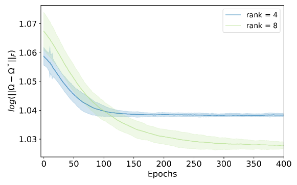
Figure 1: The choice of the optimal inferential model varies with the computational budget in a Bayesian logistic regression on the cardiac arrhythmia dataset. When the computational budget can only permit training 10 epochs, the less flexible rank-4 Gaussian inferential model (Equation 3) achieves a lower posterior approximation error, measured by the Frobenius distance between the precision matrices of the approximate and the exact posterior. With a higher computational budget (e.g. training 100 epochs), the more flexible rank-8 inferential model achieves a lower error.

The statistical and computational trade-off in variational inference suggests that choosing the most flexible inferential models can be suboptimal under a limited computational budget. Then how does statistical accuracy trade-off with computational efficiency? How can we choose the inferential model to achieve the optimal trade-off? We study these questions in this paper.

1.1 Main ideas

We describe the setup and the main results of the paper. Consider a standard statistical inference task on a dataset $\mathbf{x}=\{x_{i}\}_{i=1}^{n}$. We posit a probability model $p(\mathbf{x}\,|\,\theta)$ with a $d$-dimensional latent variable $\theta$ and a prior $p(\theta)$ on the latent. The goal is to estimate the latent variable $\theta$ by inferring its posterior $p(\theta\,|\,\mathbf{x})=p(\theta)\cdot p(\mathbf{x}\,|\,\theta)/p(\mathbf{x})$. The posterior is hard to compute because its denominator is the marginal likelihood of $\mathbf{x}$, which is an integral $p(\mathbf{x})=\int p(\theta)p(\mathbf{x}\,|\,\theta)\mathop{}\!\mathrm{d}\theta$ and is often computationally intractable.

Variational inference seeks to approximate the posterior $p(\theta\,|\,\mathbf{x})$. We first posit an inferential model $\mathcal{Q}$, also known as a variational approximating family. A classical choice of $\mathcal{Q}$ is the mean-field family, which contains all distributions with factorizable densities (Wainwright and Jordan,, 2008). After positing $\mathcal{Q}$, we then find the member within $\mathcal{Q}$ that is closest in KL divergence to the exact posterior,

$$q_{\phi^{*}}(\theta\,|\,\mathbf{x})=\operatorname*{arg\,min}_{q_{\phi}\in\mathcal{Q}}\mathrm{KL}\left(q_{\phi}(\theta\,|\,\mathbf{x})\|p(\theta\,|\,\mathbf{x})\right).$$ (1)

The closest member $q_{\phi^{*}}(\theta\,|\,\mathbf{x})$, sometimes called the variational posterior, is used in downstream analysis in the place of the exact posterior.

Variational inference circumvents the computation of the intractable integral. The reason is that Equation 1 is equivalent to maximizing an objective that does not involve the hard-to-compute integral $p(\mathbf{x})=\int p(\theta)p(\mathbf{x}\,|\,\theta)\mathop{}\!\mathrm{d}\theta$, that is,

$$q_{\phi^{*}}(\theta\,|\,\mathbf{x})=\operatorname*{argmax}_{q_{\phi}\in\mathcal{Q}}\mathbb{E}_{\theta\sim q_{\phi}(\theta\,|\,\mathbf{x})}\left[\log p(\theta,\mathbf{x})-\log q_{\phi}(\theta\,|\,\mathbf{x})\right].$$ (2)

The objective in Equation 2 is known as the evidence lower bound (ELBO), whose expectation can be calculated via Monte Carlo samples of $q_{\phi}(\theta\,|\,\mathbf{x})$.

The inferential model $\mathcal{Q}$ drives the statistical accuracy and computational efficiency of variational inference. The variational posterior is a biased estimate of the exact posterior when the inferential model $\mathcal{Q}$ is too restrictive to contain the exact posterior. Yet, such a variational posterior can be easier to compute, because searching over a more restricted inferential model is more computationally efficient. Thus, variational inference trades statistical accuracy for computational efficiency by restricting the capacity of its inferential model. Though this trade-off in variational inference is observed in empirical studies (e.g. Figure 1), few theoretical results exist around the characterization of this trade-off.

Here we theoretically characterize this statistical and computational trade-off by varying the choice of inferential models. We consider low-rank Gaussian inferential models: a rank-$p$ Gaussian inferential model is a Gaussian family for variational approximation whose precision matrix has a structure of a diagonal matrix plus a rank-$p$ matrix,

$$\mathcal{Q}_{p}=\{\mathcal{N}(\hat{\theta},\Omega^{-1}):\hat{\theta}\in\mathbb{R}^{d},\Omega=D+\sum_{i=1}^{p}\lambda_{i}u_{i}u_{i}^{\top},\text{$D$ is a $d\times d$ diagonal matrix},p\leq d\},$$ (3)

where we denote the parameters as $\phi=(\hat{\theta},\Omega).$

These low-rank inferential models extend the classical Gaussian mean-field family: the Gaussian mean-field family is a special case of $\mathcal{Q}_{p}$ with $p=0$. Unlike the mean-field family, however, this low-rank family can capture the dependence structure among latent variables. As we increase the rank $p$ to be $p=d$, $\mathcal{Q}_{p}$ becomes the Gaussian full-rank family. The rank of an inferential model indicates its capacity, so we will consider the low-rank inferential models with different $p$’s to study the statistical and computational trade-offs in variational inference.

Using this Gaussian low-rank family of inferential models, we study the statistical and computational trade-offs of variational inference in two aspects: Bayesian posterior inference error and frequentist uncertainty quantification error. Bayesian posterior inference error characterizes the error of the approximate posterior relative to the exact posterior in KL divergence.

Informal version of Theorem 1.  After running stochastic variational inference (specifically, the preconditioned SGD algorithm detailed in Section 2) with at most $\Pi$ gradient evaluations, the resulting variational posterior $q_{\phi^{(T)}}(\theta\,|\,\mathbf{x})$ satisfies

$$\mathrm{KL}\left(q_{\phi^{(T)}}(\theta\,|\,\mathbf{x})\leavevmode\nobreak\ \|\leavevmode\nobreak\ p(\theta\,|\,\mathbf{x})\right) \leq\underbrace{c_{1}\cdot\sum_{k=p+1}^{d}\left(\lambda^{*}_{k}\right)^{2}}_{\text{Variational Approximation Error}}+\underbrace{c_{2}\cdot\left(\frac{pd}{\Pi}\right)^{1/3}\sum_{k=1}^{p}\lambda^{*}_{k}}_{\text{Optimization Error}},$$ (4)

with high probability, where $\lambda^{*}_{k}$ is the $k$th largest eigenvalues of the true posterior precision; $c_{1},c_{2}$ are two constants; $T$ is the number of iterations corresponding to $\Pi$ gradient evaluations.

Theorem 1 shows that the total error of the variational posterior (i.e. the KL divergence between the variational and exact posterior) is composed of two terms, an irreducible statistical approximation error and a reducible numerical error. Lower-rank approximation of the posterior suffers from a larger irreducible statistical approximation error. Yet, its numerical error can be reduced by more computation, which scales linearly with the rank. Accordingly, a higher-rank approximation achieves lower statistical error but requires more computation to reduce the numerical error.

Theorem 1 also suggests an optimal choice of inferential model that can significantly improve the required computation budget. In particular, given a fixed error tolerance, the optimal inferential model requires a total computational budget that only scales linearly with the dimension $d$ in Equation 27, as opposed to the quadratic scaling if we use the naive full-rank parametrization (Hoffman and Ma,, 2019). Moreover, the faster the eigenvalue decay of $\lambda_{k}^{*}$ is, the less computation the optimal inferential model requires to achieve the error tolerance. Finally, the computation budget scales with the condition number of the true posterior precision.

We next turn to evaluate variational inference in its resulting frequentist uncertainty estimate, considering the covariance matrix of the variational posterior as an uncertainty estimate.

Informal version of Theorem 2.  After stochastic variational inference with at most $\Pi$ number of gradient evaluations, the precision matrix $\Omega^{(T)}$ of the resulting variational posterior satisfies

$$\left\|\frac{1}{n}\Omega^{(T)}-\Omega^{*}\right\|_{F}^{2}\leq\underbrace{c_{3}\sum_{k=p+1}^{d}(\lambda_{k}^{*})^{2}}_{\text{Variational Approximation Error}}+\underbrace{c_{4}\cdot\left(\frac{pd}{\Pi}\right)^{1/3}\sum_{k=1}^{p}\lambda^{*}_{k}}_{\text{Optimization Error}}+\underbrace{\frac{c_{5}}{n}}_{\text{Statistical Error}},$$ (5)

with high probability, where $\Omega^{*}$ is the true (rescaled) posterior precision matrix with infinite i.i.d. data, and $c_{3},c_{4},c_{5}$ are some constants.

Theorem 2 implies that, relative to the true asymptotic covariance matrix, variational inference with lower-rank inferential models bears lower computational costs (the second term) but suffers from higher approximation error (the first term). Further, when the sample size is small, the third term may dominate; thus the optimal inferential model need not be full-rank to achieve the optimal order of estimation error (even with unlimited computational budget). In particular, under unlimited computational budget, any inferential model is optimal as long as its approximation error is of (at most) the same order as the statistical error; further decreasing the approximation error with more flexible inferential models cannot decrease the order of the total error.

The key observation behind these results is the connection between the natural gradient descent algorithm commonly used in variational inference and the stochastic power method, whose convergence rate depends on the noise of the gradient (Hardt and Price,, 2014). Specifically, this connection implies that the convergence rate of variational inference also depends on the noise of its gradients, which increases as we increase the flexibility of the inferential model $\mathcal{Q}$. In more detail, the gradient of the ELBO decomposes into two terms

$$\nabla_{\phi}\mathbb{E}_{\theta\sim q_{\phi}(\theta\,|\,\mathbf{x})}\left[\log p(\theta,\mathbf{x})-\log q_{\phi}(\theta\,|\,\mathbf{x})\right]\\ =-\mathbb{E}_{\theta\sim q_{\phi}(\theta\,|\,\mathbf{x})}\left[\nabla_{\phi}\log q_{\phi}(\theta\,|\,\mathbf{x})\cdot\log{q_{\phi}(\theta\,|\,\mathbf{x})}\right]+\mathbb{E}_{\theta\sim q_{\phi}(\theta\,|\,\mathbf{x})}\left[\nabla_{\phi}\log q_{\phi}(\theta\,|\,\mathbf{x})\cdot\log p(\theta,\mathbf{x})\right].$$

The first term can be computed deterministically. The second term, however, can only be estimated via drawing samples from $\theta\sim q_{\phi}(\theta\,|\,\mathbf{x})$, and induce noise in gradients; this noise increases as the inferential model becomes more flexible, i.e. $\mathcal{Q}$ has a higher-rank precision matrix.

Beyond theoretical understanding, Theorems 1 and 2 can also inform optimal inferential model selection in practice, which we demonstrate in Section 4. We also corroborate the theoretical findings with empirical studies. Across synthetic experiments, we find that empirical observations confirm the theoretical results: higher-rank approximation exhibits better statistical accuracy but takes more stochastic gradient steps to converge.

Related work.  This work draws on several threads of previous research in theoretical characterizations of variational inference and statistical–computational trade-offs in statistical methods.

Theoretical results around variational inference have mostly centered around its statistical properties, including asymptotic properties (Wang and Blei,, 2018, 2019; Chérief-Abdellatif,, 2020; Chen and Ryzhov,, 2020; Knoblauch,, 2019; Bhattacharya and Maiti,, 2021; Bhattacharya et al.,, 2020; Hajargasht,, 2019; Han and Yang,, 2019; Guha et al.,, 2020; Banerjee et al.,, 2021; Chérief-Abdellatif,, 2019; Jaiswal et al.,, 2020; Chérief-Abdellatif et al.,, 2018; Womack et al.,, 2013; Hall et al., 2011a, ; Hall et al., 2011b, ; Celisse et al.,, 2012; Bickel et al.,, 2013; Westling and McCormick,, 2015; You et al.,, 2014; Wang et al.,, 2006; Zhang and Gao,, 2017; Wang and Titterington,, 2004; Pati et al.,, 2017; Yang et al.,, 2017; Alquier and Ridgway,, 2017; Alquier et al.,, 2016; Campbell and Li,, 2019), finite sample approximation error (Huggins et al.,, 2018, 2020; Giordano et al.,, 2017; Sheth and Khardon,, 2017; Chen et al.,, 2017), robustness to model misspecification (Medina et al.,, 2021; Chérief-Abdellatif et al.,, 2018; Wang and Blei,, 2019; Alquier and Ridgway,, 2017), and properties in high-dimensional settings (Ray and Szabó,, 2021; Yang and Martin,, 2020; Ray et al.,, 2020; Mukherjee and Sen,, 2021). Beyond statistical properties, a few works have explored the role of optimization algorithms in variational inference (Mukherjee and Sarkar,, 2018; Sarkar et al.,, 2021; Plummer et al.,, 2020; Zhang and Zhou,, 2017; Ghorbani et al.,, 2018; Hoffman and Ma,, 2020; Xu and Campbell,, 2021). Along this line, closest to our work is Xu and Campbell, (2021), which investigates the asymptotic properties of the nonconvex optimization problem in Gaussian variational inference. Our work differs from these works: we focus on explicitly characterizing the statistical and computational trade-offs in variational inference, enabling us to identify the optimal choice of inferential model that strikes the balance.

Despite being rarely explored in variational inference, statistical and computational trade-offs have been formalized in other statistical problems, including principal component analysis (Wang et al.,, 2016; Sriperumbudur and Sterge,, 2017), clustering (Calandriello and Rosasco,, 2018; Balakrishnan et al.,, 2011), matrix completion (Dasarathy et al.,, 2017), denoising problems (Chandrasekaran and Jordan,, 2013), high-dimensional problems (Berthet et al.,, 2014), single-index models (Wang et al.,, 2019), two-sample testing (Ramdas et al.,, 2015), weakly supervised learning (Yi et al.,, 2019), combinatorial problems (Lu et al.,, 2018; Khetan and Oh,, 2016; Jin et al.,, 2020; Khetan and Oh,, 2018), and other estimators like stochastic composite likelihood (Dillon and Lebanon,, 2009) and Dantzig-type estimators (Li et al.,, 2016). These analyses focus on studying point estimators for the parameters of interest. In contrast, we consider distributional estimators in this work. We characterize the statistical and computational trade-offs for variational posterior distributions.

Finally, this work relates to the body of literature on Bayesian model selection; see O’Hara et al., (2009) for a review. Closely related works include Chandrasekaran et al., (2010) which focuses on identifiability and tractability of latent variable model selection, Yang et al., (2016) which analyzes an MCMC approach to Bayesian variable selection based on designing priors, and Song et al., (2020) which proposes an extended stochastic gradient MCMC for Bayesian variable selection. These works analyze different aspects of Bayesian model selection algorithms than we do; they focus on identifiability, asymptotic convergence, or computational complexity, while we analyze non-asymptotic convergence and statistical guarantees.

This paper.  The rest of the paper is organized as follows. Section 2 introduces the optimization algorithms we analyze for stochastic variational inference. In Section 3, we analyze the convergence of stochastic variational inference for Gaussian posteriors, via transforming it into an equivalent algorithm that performs the stochastic power method. In Section 4, we study the statistical and computational trade-offs in stochastic variational inference. We first focus on the Bayesian posterior inference error, measured by KL divergence between the variational approximation and the true posterior. We then examine the frequentist uncertainty quantification error, where the precision matrix of the inferential model is used to quantify the sampling uncertainty. In both cases, we demonstrate how the theoretical results inform optimal inferential model selection: they identify the optimal rank $p$ of the low-rank inferential model so that they achieve a given error threshold with minimum total computation. In Section 5, we extend the convergence analysis of Section 3 beyond Gaussian posteriors and analyze the inference error due to the low-rank inferential model. We conclude with empirical studies in Section 6.

Stochastic Optimization for Variational Inference

To study the statistical and computational trade-off in variational inference, we first study the stochastic optimization algorithms, focusing on their convergence behaviors in variational inference with low-rank Gaussian inferential models. In the next section, we will discuss the implications of these convergence behaviors on the statistical and computational trade-off in variational inference.

2.1 Stochastic variational inference (SVI) algorithm

Recall that our goal is to find a variational approximation $q(\theta|\mathbf{x})$ to the posterior within an inferential model, a.k.a. a variational approximating family. We focus on the family of rank-$p$ Gaussian inferential model $\mathcal{Q}_{p}$; all members of $\mathcal{Q}_{p}$ are multivariate Gaussian $\mathcal{N}(\hat{\theta},\Omega^{-1})$ with a diagonal plus rank-$p$ precision matrix: $\Omega=D+\sum_{i=1}^{p}\lambda_{i}u_{i}u_{i}^{\top}=D+U\Lambda U^{\top}$, where $U\in\mathbb{R}^{d\times p}$ is a semi-orthonormal matrix and its associated eigenvalues are $\Lambda\in\mathbb{R}^{p\times p}$. For simplicity of exposition, we assume that this Gaussian inferential model is centered with $\hat{\theta}=0$ and the diagonal structure of its precision matrix is contributed by an isotropic normal prior, i.e. $D=\alpha\mathrm{I}_{d}$. The discussion easily extends to non-centered $\hat{\theta}$ and anisotropic $D$.

To find the closest variational approximation in $\mathcal{Q}_{p}$, we solve an optimization problem that minimize $\mathrm{KL}\left(q(\theta\,|\,\mathbf{x})\leavevmode\nobreak\ \|\leavevmode\nobreak\ p(\theta\,|\,\mathbf{x})\right)$—often abbreviated to $\mathrm{KL}\left(q\leavevmode\nobreak\ \|\leavevmode\nobreak\ p\right)$—subject to the constraint that $q(\theta\,|\,\mathbf{x})\in\mathcal{Q}_{p}.$ The most common approach to this optimization is to perform gradient descent over the KL divergence to find the optimal parameters for the variational approximation. Specifically, we write $q_{(U,\Lambda)}$ as the variational approximation with parameters $U$ and $\Lambda$, and perform gradient descent over $\mathrm{KL}\left(q\leavevmode\nobreak\ \|\leavevmode\nobreak\ p\right)$ with respect to the parameters $\phi\in\{u_{i},\lambda_{i}\}_{i=1}^{p}$,

$$\nabla_{\phi}\mathrm{KL}\left(q\leavevmode\nobreak\ \|\leavevmode\nobreak\ p\right) =\mathbb{E}_{\theta\sim q}\left[\nabla_{\phi}\log q_{(U,\Lambda)}(\theta|\mathbf{x})\log\frac{q_{(U,\Lambda)}(\theta|\mathbf{x})}{p(\theta|\mathbf{x})}\right].$$ (6)

The gradient $\nabla_{\phi}\mathrm{KL}\left(q\leavevmode\nobreak\ \|\leavevmode\nobreak\ p\right)$ can be further decomposed into two terms,

$$\nabla_{\phi}\mathrm{KL}\left(q\leavevmode\nobreak\ \|\leavevmode\nobreak\ p\right)=\mathbb{E}_{\theta\sim q}\left[\nabla_{\phi}\log q_{(U,\Lambda)}(\theta|\mathbf{x})\cdot\log{q_{(U,\Lambda)}(\theta|\mathbf{x})}\right]+\mathbb{E}_{\theta\sim q}\left[\nabla_{\phi}\log q_{(U,\Lambda)}(\theta|\mathbf{x})\cdot\psi(\theta)\right],$$ (7)

where we denote $\psi(\theta)$ as the unnormalized component of the true posterior, $p(\theta|\mathbf{x})\propto\exp\left(-\psi(\theta)\right)$ with $\psi(\theta)$ being a positive definite function. (Equation 7 is due to integration by parts, which implies that $\mathbb{E}_{\theta\sim q}\left[\nabla_{\phi}\log q_{(U,\Lambda)}(\theta|\mathbf{x})\cdot C\right]=0$ for any constant $C$.) The decomposition in Equation 7 implies that its first term has a closed form and can be explicitly computed for $q\in\mathcal{Q}_{p}$ from the low-rank Gaussian inferential model. The second term, in contrast, does not always have a closed form. As it is an expectation over $q_{(U,\Lambda)}(\ \cdot\ |\mathbf{x})$, we often adopt a Monte Carlo estimate

$$\mathbb{E}_{\theta\sim q}\left[\nabla_{\phi}\log q_{(U,\Lambda)}(\theta|\mathbf{x})\cdot\psi(\theta)\right]\approx\frac{1}{N}\sum_{j=1}^{N}\nabla_{\phi}\log q_{(U,\Lambda)}(\theta_{j}|\mathbf{x})\cdot\psi(\theta_{j}),$$

where $\theta_{j}$ are i.i.d. samples from $q_{(U,\Lambda)}(\ \cdot\ |\mathbf{x})$; the variance of this Monte Carlo estimate decreases with larger $N$.

In practice, we often perform gradient descent in two stages. We first learn the semi-orthonormal matrix $U=[u_{1},\ldots,u_{p}]$ and then proceed to learn the corresponding eigenvalues $\Lambda=\mathrm{diag}(\lambda_{1},\ldots,\lambda_{p})$. Below we detail the stochastic optimization algorithm for $U$ and $\Lambda$ respectively.

Optimizing for the eigenvectors $U$.  In the first stage of the algorithm, we focus on optimizing the semi-orthonormal matrix $U$, fixing the other parameters $\Lambda$ at their initial values, e.g. $\Lambda^{(0)}\leavevmode\nobreak\ =\leavevmode\nobreak\ \mathrm{I}_{p}$.

To optimize $U$, we perform preconditioned gradient descent of KL divergence over $U$ (Dennis and Schnabel,, 1983). We employ the preconditioner $\mathrm{I}\otimes\Omega$ such that the preconditioned gradient of the KL divergence has a simple form,

$$\Omega\nabla_{U}\mathrm{KL}\left(q\leavevmode\nobreak\ \|\leavevmode\nobreak\ p\right) =U\Lambda+\mathbb{E}_{\theta\sim q}\left[\left(-\Omega\theta\theta^{\top}U\Lambda+U\Lambda\right)\psi(\theta)\right]$$ (8)

$$=U\Lambda-\mathbb{E}_{\theta\sim q}\left[\nabla\psi(\theta)\theta^{\top}\right]U\Lambda,$$ (9)

where Equation 8 is obtained by calculating $\nabla_{U}\log q_{(U,\Lambda)}(\theta|\mathbf{x})=-\theta\theta^{\top}U\Lambda+\Omega^{-1}U\Lambda$ and plugging it into Equation 7. Thus, given the eigenvalues $\Lambda$, the preconditioned stochastic gradient descent (SGD) over $U$ operates as follows. At the $t$th iteration,

$$\text{Sample i.i.d.}\;\theta_{j}^{(t)}\sim q_{\left(U^{(t)},\Lambda\right)},j\in\{1,\dots,N\},$$ (10)

$$\tilde{U}^{(t+1)}=U^{(t)}-h_{t}U^{(t)}\Lambda+\frac{h_{t}}{N}\sum_{j=1}^{N}\left(\nabla\psi\left(\theta_{j}^{(t)}\right)\theta_{j}^{\top}\right)U^{(t)}\Lambda,$$ (11)

$$U^{(t+1)}=\mathrm{QR}\left(\tilde{U}^{(t+1)}\right),$$ (12)

where $\Omega^{(t)}=D+U^{(t)}\Lambda\left(U^{(t)}\right)^{\top}$. Equation 12 employs a QR decomposition to ensure that the matrix $U^{(t)}$ is a semi-orthonormal matrix at all iterations. We choose a simple initialization: $U^{(0)}=[e_{1},\dots,e_{p}]$, where $e_{i}\in\mathbb{R}^{d}$ is a column vector with $1$ in the $i$-th entry and $0$’s elsewhere.

Input: $D=\alpha\mathrm{I}$, $U^{(0)}=\left[e_{1},\dots,e_{p}\right]$, $\Lambda^{(0)}=\mathrm{I}_{p}$

for $t=0,\ldots,T-1$ do

      

$$\text{Sample i.i.d.}\;\theta_{j}^{(t)}\sim q_{\left(U^{(t)},\Lambda^{(t)}\right)},\forall j\in\{1,\dots,N\},$$

$$\tilde{U}^{(t+1)}=U^{(t)}-h_{t}U^{(t)}\Lambda^{(t)}+\frac{h_{t}}{N}\sum_{j=1}^{N}\left(\nabla\psi\left(\theta_{j}^{(t)}\right)\theta_{j}^{\top}\right)U^{(t)}\Lambda^{(t)},$$

$$U^{(t+1)}=\mathrm{QR}\left(\tilde{U}^{(t+1)}\right).$$

Sample i.i.d. $\theta_{j}^{(t)}\sim q_{\left(U^{(t)},\Lambda^{(t)}\right)},\forall j\in\{1,\dots,M\}$.

       for $k=1,\dots,p$ do

            

$$\lambda^{(t)}_{k}=\frac{1}{M}\sum_{j=1}^{M}\left(u_{k}^{(t)}\right)^{\top}\left(\frac{\nabla\psi(\theta_{j}+\Delta\cdot u_{k}^{(t)})-\nabla\psi(\theta_{j}-\Delta\cdot u_{k}^{(t)})}{2\Delta}\right)-D_{k,k}.$$ (13)

       end for

      

end for

Return: $U^{(T)},\Lambda^{(T)}=\mathrm{diag}(\lambda^{(T)}_{1},\ldots,\lambda^{(T)}_{p})$

Algorithm 1 Stochastic variational inference (SVI) with low-rank Gaussian inferential models

Optimizing for the eigenvalues $\Lambda$.  In the second stage of the algorithm, we learn the diagonal eigenvalue matrix $\Lambda$ given the estimated semi-orthonormal matrix $U$. We find the optimal $\Lambda$ by finding the values of $\lambda_{i}$ achieving a zero derivative of the log-likelihood over $\lambda_{i}$. In the following lemma, we obtain an explicit expression for solving $\lambda_{i}$, given vector $u_{i}$ in the semi-orthonormal matrix $U$.

Lemma 1.

The solution to $\nabla_{\lambda_{i}}\mathrm{KL}\left(q_{(U,\Lambda)}(\theta|\mathbf{x})\leavevmode\nobreak\ \|\leavevmode\nobreak\ p(\theta|\mathbf{x})\right)=0$ is $\lambda_{i}=\mathbb{E}_{\theta\sim q}\left[u_{i}^{\top}\nabla_{\theta}^{2}\psi(\theta)u_{i}\right]-D_{i,i}$.

This fact implies that solving for optimal $\lambda_{i}$ is equivalent to evaluating $\mathbb{E}_{\theta\sim q}\left[u_{i}^{\top}\nabla_{\theta}^{2}\psi(\theta)u_{i}\right]$, which we use $M$ samples of $\theta\sim q$ to estimate. We then note that the Hessian vector product $\nabla_{\theta}^{2}\psi(\theta)u_{i}$ can be accurately estimated by the gradient difference: $\left(\nabla\psi(\theta+\Delta\cdot u_{i})-\nabla\psi(\theta-\Delta\cdot u_{i})\right)/\left(2\Delta\right)$. Combining these two facts yields the update rule of Equation 13 in Algorithm 1.

Taken together the two stages of optimization, Algorithm 1 summarizes the full stochastic optimization algorithm for variational inference with low-rank Gaussian inferential models.

Convergence analysis of SVI for Gaussian posteriors

We next analyze the non-asymptotic convergence properties of the SVI algorithm in Algorithm 1. This analysis will characterize the computational properties of variational inference and facilitate the characterization of statistical and computational trade-offs in Section 4. As in Section 2, we focus on the Gaussian posterior cases in Section 3 and Section 4, where we can express the posterior as $p(\theta|{\bf x})\propto\exp\left(-\psi(\theta)\right)$, where $\psi(\theta)=\frac{1}{2}\theta^{\top}\Omega^{(\infty)}\theta$ for a positive definite matrix $\Omega^{(\infty)}\in\mathbb{R}^{d\times d}$. (We extend to non-Gaussian cases in Section 5.)

To analyze Algorithm 1 for the Gaussian posterior (corresponding to a quadratic function $\psi$), we rely on a key observation that the learning of $U$ and $\Lambda$ decouples: the optimization algorithm does not require we alternate between optimizing $U$ and $\Lambda$; rather, it can be separated into two separate stages because the optimization of $U$ does not depend on the value of $\Lambda$ in variational inference with low-rank Gaussian inferential models. In particular, the update in Equation 11, together with the QR decomposition in Equation 12, implies that the stationary solution to the semi-orthonormal $U$ is always composed of the first $p$ eigenvectors of $\Omega^{(\infty)}$, regardless of the choice of $\Lambda$ in the update. From Lemma 1, we also know that, if the eigenspace $U$ is learned, then the solution $\Lambda$ simply reads out the eigenvalues of $\mathbb{E}_{\theta\sim q}\left[\nabla^{2}\psi(\theta)\right]$, which is $\Omega^{(\infty)}$ in the Gaussian posterior case. Therefore, the optimization of $U$ and $\Lambda$ can be performed in two stages by first fixing $\Lambda=\mathrm{I}_{p}$ and letting $U$ converge first and then computing $\Lambda$ conditioning on $U$.

These observations enables us to consider Algorithm 2 (SVI_Gauss)—a simplified version of Algorithm 1 tailored to Gaussian posteriors—to facilitate the analysis for Gaussian posteriors in Section 4. (The details of Algorithm 2 is in Appendix A.) Moreover, as we will see, the update of $U$ in Algorithm 2 (SVI_Gauss) closely connects to the stochastic power method (Hardt and Price,, 2014); this connection will allow us to borrow analysis tools of the stochastic power method for analyzing stochastic optimization for variational inference. Below we discuss these observations and connections in detail.

SVI and the stochastic power method.  To establish the connection between the stochastic power method and the SVI algorithm, we prove that the first stage of Algorithm 1—which performs preconditioned SGD to optimize for the eigenvectors $U$—is equivalent to the stochastic power method for principal component analysis (PCA).

Lemma 2 (SVI $\Leftrightarrow$ Stochastic power method).

Suppose the diagonal matrix $D=\alpha\mathrm{I}_{d}$ and fix $\Lambda=\mathrm{I}_{p}$ in the update of the matrix $U^{(t)}$ in Algorithm 1 (Equation 10–Equation 12). The preconditioned SGD in Equations 10, 11 and 12 with step size $h_{t}=1$ is equivalent to the stochastic power method:

$$\text{Sample i.i.d.}\;\theta_{j}^{(t)}\sim\mathcal{N}\left(0,(\Omega^{(t)})^{-1}\right),\forall j\in\{1,\dots,N\},$$ (14)

$$\tilde{U}^{(t+1)}=\sum_{j=1}^{N}\left(\nabla\psi\left(\theta_{j}^{(t)}\right)\left(\theta_{j}^{(t)}\right)^{\top}\Omega^{(t)}\right)U^{(t)},$$ (15)

$$U^{(t+1)}=\mathrm{QR}\left(\tilde{U}^{(t+1)}\right),$$ (16)

where $\Omega^{(t)}=D+U^{(t)}\Lambda\left(U^{(t)}\right)^{{\top}}=\alpha\mathrm{I}_{d}+U^{(t)}\left(U^{(t)}\right)^{\top}$.

In addition, for the Gaussian posterior, Algorithm 2 (which substitutes $\Omega^{(t)}$ in Equation 14 and Equation 15 with a fixed input matrix $\Omega$) yields the same stationary solution $U$ as that of the above update, for any positive definite input $\Omega$.

Lemma 2 is an immediate consequence of equating the updates (Equations 10, 11 and 12 and Equations 14, 15 and 16) in both algorithms. Hence for Gaussian posteriors, we can directly analyze Algorithm 2 for the convergence of Algorithm 1.

Convergence analysis of SVI.  Lemma 2 established the equivalence between the first stage of Algorithm 1 and the stochastic power method. Existing works on the stochastic power method discover that, even though the objective is nonconvex, with small enough noise during each iteration, the algorithm will converge and approximately recover the top $p$ eigenspace of $\Omega^{(\infty)}$. Leveraging this connection, below we study the convergence properties of Algorithm 1 for each of its two stages and establish per-iteration noise bounds to determine number of samples to generate in the sampling step (Equation 30) of Algorithm 2.

We first establish the convergence of the first stage of Algorithm 1 that optimizes over the $d\times p$ semi-orthonormal matrix $U$. For the Gaussian posterior $p(\theta|{\bf x})\propto\exp\left(-\psi(\theta)\right)$, if function $\psi=\frac{1}{2}\theta^{\top}\Omega^{(\infty)}\theta$ is $\alpha$-strongly convex, then we can express $\Omega^{(\infty)}=U^{(\infty)}\Lambda^{(\infty)}\left(U^{(\infty)}\right)^{\top}+\alpha\mathrm{I}$, for unitary matrix $U^{(\infty)}\in\mathbb{R}^{d\times d}$ and positive semi-definite diagonal matrix $\Lambda^{(\infty)}=\mathrm{diag}\left(\lambda^{(\infty)}_{1},\dots,\lambda^{(\infty)}_{d}\right)\in\mathbb{R}^{d\times d}$; $\alpha$ is the minimum eigenvalue of $\Omega^{(\infty)}$. For the general non-Gaussian posteriors, we will let $\alpha=\inf_{\theta\in\mathbb{R}^{d}}\min_{i=1,\dots,d}\sigma_{i}(\nabla^{2}\psi(\theta))$ to be the minimum eigenvalue of the Hessian of the negative log posterior $\nabla^{2}\psi(\theta)$ across the space $\mathbb{R}^{d}$ (See Section 5).

In what follows, we will measure the accuracy of the semi-orthonormal matrix $U=[u_{1},\dots,u_{p}]$ via the Rayleigh quotient: $u_{k}^{\top}\Omega^{(\infty)}u_{k}$ for all $k\in\left\{1,\dots,p\right\}$. A uniformly large (and close to $\lambda_{k}^{(\infty)}+\alpha$) Rayleigh quotient means that matrix $U$ is close to covering the top $p$ eigenspace of $\Omega^{(\infty)}$. Denoting $U^{(\infty)}_{p}=\left[u^{(\infty)}_{1},\dots,u^{(\infty)}_{p}\right]$ which contains the top $p$ eigenvectors of $U^{(\infty)}$, we have the following result.

Proposition 1 (Convergence of SVI over $U$).

Assume that $\psi(\theta)=\frac{1}{2}\theta^{\top}\Omega^{(\infty)}\theta$ (so that the posterior $p(\theta|{\bf x})$ is Gaussian) and is $\alpha$-strongly convex and $L$-Lipschitz smooth; the matrix $\Omega^{(\infty)}$ has condition number $\kappa(\Omega^{(\infty)})=L/\alpha.$ We run the SVI algorithm (described in in equations (14) to (16) and in Algorithm 2) for the Gaussian posterior with input matrix $\Omega$. Let $m_{0}=\sigma_{\min}\left((U^{(\infty)}_{p})^{\top}U^{(0)}\right)$ denote the initial condition. For any $\epsilon,\delta>0$, with number of stochastic gradient samples per iteration $N=\widetilde{\boldsymbol{\Omega}}\left(\max\left\{\frac{pd}{m_{0}^{2}},\frac{p^{2}}{m_{0}^{4}}\right\}\cdot\frac{L^{2}}{\alpha^{2}}\cdot\frac{L^{2}}{\epsilon^{2}}\cdot\frac{\kappa(\Omega)}{\sqrt{\delta}}\right)$, and number of iterations $T=\boldsymbol{\Theta}\left(\frac{L}{\epsilon}\log\frac{1}{m_{0}}\right)$, we obtain that

$$\left(u^{(T)}_{k}\right)^{\top}\Omega^{(\infty)}u^{(T)}_{k}\geq\lambda^{(\infty)}_{k}+\alpha-2\epsilon,\qquad\forall k\in\{1,\dots,p\}$$ (17)

with probability $1-\delta$, where $\Omega^{(\infty)}=U^{(\infty)}\Lambda^{(\infty)}\left(U^{(\infty)}\right)^{\top}+\alpha\mathrm{I}$ with minimum eigenvalue $\alpha$.

The proof of Proposition 1 is in Section B.1. The key proof idea is that we first obtain high probability bound of the distance between the gradient estimate $\frac{1}{N}\sum_{j=1}^{N}\left(\nabla\psi\left(\theta_{j}^{(t)}\right)\theta_{j}^{\top}\right)U^{(t)}$ and the true gradient $\mathbb{E}_{\theta\sim q}\left[\nabla\psi(\theta)\theta^{\top}\right]U$. This helps us decide the number of samples $N$ to generate in the first step of the algorithm. We then recursively bound how much does the top $k$ eigenspace of the $t$-th iterate: $\left[u_{1}^{(t)},\dots,u_{k}^{(t)}\right]$ overlap with the bottom eigenspace of $\Omega^{(\infty)}$ in Proposition 3, adopting similar techniques as in the analysis of stochastic power method (Hardt and Price,, 2014; balcan2016improved). Summing up the inner products between $u_{k}^{(T)}$ and the eigenvectors of $\Omega^{(\infty)}$ yields the result. (The additive term of $\alpha$ on the right side of Equation 17 is due to $\alpha$ being the minimum eigenvalue of $\Omega^{(\infty)}$.

Proposition 1 provides the scaling of the total computation complexity of the preconditioned SGD over the semi-orthonormal matrix $U$. Let $\bar{U}^{(\infty)}_{p\times p}\in\mathbb{R}^{p\times p}$ denote the $p\times p$ leading principal submatrix of $U^{(\infty)}$. Then we have $m_{0}=\sigma_{\min}\left(\bar{U}^{(\infty)}_{p\times p}\right)$ according to our choice of initialization. Assuming that $\sigma_{\min}\left(\bar{U}^{(\infty)}_{p\times p}\right)>0$, we have $N=\widetilde{\boldsymbol{\Omega}}\left(pd\cdot\frac{L^{2}}{\alpha^{2}}\cdot\frac{L^{2}}{\epsilon^{2}}\cdot\frac{\kappa(\Omega)}{\sqrt{\delta}}\right)$ and $T=\widetilde{\boldsymbol{\Theta}}\left(\frac{L}{\epsilon}\right)$. Taking the input matrix $\Omega=\mathrm{I}$, the total computation complexity of the optimization step over $U$ is $N\cdot T=\widetilde{\boldsymbol{\Omega}}\left(pd\cdot\frac{L^{2}}{\alpha^{2}}\cdot\frac{L^{3}}{\epsilon^{3}\sqrt{\delta}}\right)$.

We next analyze the second stage of the SVI algorithm which solves for $\Lambda$. We quantify the error of the resulting $\Lambda$, assuming that Proposition 1 stands and that the first stage recovers a good representation for the top $p$ eigenspace in $U$.

Proposition 2 (Convergence of SVI over $\Lambda$).

Assume the conditions for Proposition 1 are satisfied such that Equation 17 holds. Then taking the number of samples for eigenvalue computation $M\geq 2p\log(4p/\delta)\cdot\frac{L^{2}}{\epsilon^{2}}$ and $\varDelta\leq\epsilon/\left(\sqrt{p}\cdot L_{\rm{Hess}}\right)$ in Algorithm 1 Equation 13 (or Algorithm 2 Equation 33), we obtain that for Gaussian posterior,

$$\sum_{k=1}^{p}\left(\lambda^{(\infty)}_{k}-\lambda^{(T)}_{k}\right)^{2}\leq 2\sum_{k=p+1}^{d}\left(\lambda^{(\infty)}_{k}\right)^{2}+8\epsilon\sum_{k=1}^{p}\lambda^{(\infty)}_{k}+8\epsilon^{2},$$

with probability $1-\delta$.

The proof of Proposition 2 is in Section B.2. Similar to the proof of Proposition 1, we first bound the stochastic gradient noise in estimating $\mathbb{E}_{\theta\sim q}\left[u_{i}^{\top}\nabla_{\theta}^{2}\psi(\theta)u_{i}\right]$, which according to Proposition 2 achieves the critical point of $\mathrm{KL}\left(q_{(U,\Lambda)}(\theta|\mathbf{x})\leavevmode\nobreak\ \|\leavevmode\nobreak\ p(\theta|\mathbf{x})\right)$ if $u_{i}$ is the $i$-th eigenvector of $\Omega^{(\infty)}$. We then note that the gradient difference in Algorithm 2 gives an accurate estimate of the Hessian vector product $\nabla_{\theta}^{2}\psi(\theta)u_{i}$. Combining with Proposition 1 that matrix $U$ approximately recovers the top $p$ eigenspace of $\Omega^{(\infty)}$, we obtain the result.

Propositions 1 and 2 imply that the total computation complexity for the SVI algorithm to achieve $\boldsymbol{\mathcal{O}}(\epsilon)$ convergence (plus bias) is $N\cdot T+2M=\widetilde{\boldsymbol{\Omega}}\left(pd\cdot\frac{L^{2}}{\alpha^{2}}\cdot\frac{L^{3}}{\epsilon^{3}\sqrt{\delta}}\right)$. Moreover, they imply that the bound on $M$ is less than that on $N$ and that the overall complexity is dominated by the computation complexity of the preconditioned SGD over $U$. The two propositions will help us characterize how far the variational approximation is from the true posterior given fixed computational cost.

Statistical and Computational Trade-offs in Variational Inference

Leveraging the analysis of the SVI algorithm in Section 3, we characterize the non-asymptotic error of the variational posterior $q_{\left(U^{(T)},\Lambda^{(T)}\right)}(\theta\,|\,\mathbf{x})$ after $T$ steps of gradient descent. This non-asymptotic error will come from two sources: the variational approximation error due to the low-rank inferential model, and the computational error due to the stochastic optimization algorithm. How the two sources contribute to the total error of $q_{\left(U^{(T)},\Lambda^{(T)}\right)}(\theta\,|\,\mathbf{x})$ thus depicts the statistical and computational trade-offs in variational inference.

Specifically, we evaluate the variational posterior at step $T$, $q_{\left(U^{(T)},\Lambda^{(T)}\right)}(\theta\,|\,\mathbf{x})$, from two aspects: Bayesian posterior inference and frequentist uncertainty quantification. For simplicity of exposition, we adopt the setting where the exact posterior is a centered Gaussian, i.e. $p(\theta\,|\,\mathbf{x})=\mathcal{N}(0,(\Omega^{(\infty)})^{-1})$ for some $\Omega^{(\infty)}$. Locating the mean parameter requires much less computation; hence this simplication does not alter the analysis. The Gaussianity of the exact posterior simplifies the SVI algorithm to Algorithm 2. (We extend to general non-Gaussian posteriors in Section 5.)

4.1 Bayesian posterior inference error

We first study the Bayesian posterior inference error of variational posteriors, where we evaluate its KL divergence to the true Bayesian posterior, $\mathrm{KL}\left(q_{\left(U^{(T)},\Lambda^{(T)}\right)}(\theta\,|\,\mathbf{x})\leavevmode\nobreak\ \|\leavevmode\nobreak\ p(\theta\,|\,\mathbf{x}))\right)$.

Combining the convergence analysis of both stages of Algorithm 1 in Section 3, the following theorem establishes the computation-approximation trade-off. To focus on how the error depends on the rank $p$ of the inferential model, below we adopt the initialization of $U^{(0)}=\left[e_{1},\dots,e_{p}\right]$ and that $m_{0}=\sigma_{\min}\left(\bar{U}^{(\infty)}_{p\times p}\right)>0$.

Theorem 1.

Suppose that we are given a computation budget that allows for $\Pi=N\cdot T+2M$ gradient evaluations in Algorithm 1 with input matrix $\Omega=\mathrm{I}$. Then under the allocation rule of $N=\boldsymbol{\Theta}\left(\Pi^{2/3}\cdot\frac{(pd)^{1/3}}{\delta^{1/6}}\cdot\left(\frac{L}{\alpha}\right)^{2/3}\right)$, $T=\boldsymbol{\Theta}\left(\Pi^{1/3}\cdot\frac{\delta^{1/6}}{(pd)^{1/3}}\cdot\left(\frac{\alpha}{L}\right)^{2/3}\right)$, and $M=\widetilde{\boldsymbol{\Theta}}\left(\Pi^{2/3}\cdot\frac{p^{1/3}}{d^{2/3}}\cdot\left(\frac{\alpha}{L}\right)^{4/3}\delta^{1/3}\right)$ (also laid out in Proposition 1 and Proposition 2), the variational posterior $q_{\left(U^{(T)},\Lambda^{(T)}\right)}(\theta\,|\,\mathbf{x})$ satisfies

$$\mathrm{KL}\left(q_{\left(U^{(T)},\Lambda^{(T)}\right)}(\theta\,|\,\mathbf{x})\leavevmode\nobreak\ \|\leavevmode\nobreak\ p(\theta\,|\,{\bf x})\right) \lesssim\underbrace{\frac{1}{\alpha^{2}}\sum_{k=p+1}^{d}\left(\lambda^{(\infty)}_{k}\right)^{2}}_{E_{1}:\text{ Approximation}}+\underbrace{\left(\frac{pd}{\Pi}\right)^{1/3}\cdot\left(\frac{L}{\alpha}\right)^{5/3}\cdot\frac{1}{\delta^{1/6}}\cdot\frac{1}{\alpha}\sum_{k=1}^{p}\lambda^{(\infty)}_{k}}_{E_{2}:\text{ Optimization}},$$ (18)

with $(1-\delta)$ probability, where we have the exact posterior satisfying $p(\theta\,|\,\mathbf{x})\propto\exp\left(-\theta^{\top}\Omega^{(\infty)}\theta\right)$ with $\Omega^{(\infty)}=\alpha\mathrm{I}_{d}+U^{(\infty)}\Lambda^{(\infty)}\left(U^{(\infty)}\right)^{\top}$ and $\alpha$ being the minimum eigenvalue of $\Omega^{(\infty)}$.

Alternatively, we can express the result that with the number of stochastic gradient samples per iteration $N=\widetilde{\boldsymbol{\Omega}}\left(\max\left\{\frac{pd}{m_{0}^{2}},\frac{p^{2}}{m_{0}^{4}}\right\}\cdot\frac{L^{2}}{\alpha^{2}}\cdot\frac{L^{2}}{\epsilon^{2}\sqrt{\delta}}\right)$, the number of iterations $T=\boldsymbol{\Theta}\left(\frac{L}{\epsilon}\log\frac{1}{m_{0}}\right)$, as well as the number of samples for eigenvalue computation $M={\boldsymbol{\Omega}}\left(p\log(p/\delta)\cdot\frac{L^{2}}{\epsilon^{2}}\right)$,

$$\mathrm{KL}\left(q_{\left(U^{(T)},\Lambda^{(T)}\right)}(\theta\,|\,\mathbf{x})\leavevmode\nobreak\ \|\leavevmode\nobreak\ p(\theta\,|\,{\bf x})\right) \leq\frac{1}{2\alpha^{2}}\left\|\Omega^{(\infty)}-\Omega^{(T)}\right\|_{F}^{2}$$

$$\leq\underbrace{\frac{3}{2\alpha^{2}}\sum_{k=p+1}^{d}\left(\lambda^{(\infty)}_{k}\right)^{2}}_{E_{1}:\text{ Approximation}}+\underbrace{\frac{6}{\alpha^{2}}\epsilon\sum_{k=1}^{p}\lambda^{(\infty)}_{k}+\frac{4\epsilon^{2}}{\alpha^{2}}}_{E_{2}:\text{ Optimization}}.$$ (19)

The proof of Theorem 1 is in Appendix B. The key idea of the proof is to combine the convergence analyses of Propositions 1 and 2 and obtain an upper bound on the Frobenius norm difference $\left\|\Omega^{(\infty)}-\Omega^{(T)}\right\|_{F}$ via the difference in the eigenvalues of $\Omega^{(\infty)}$ and $\Omega^{(T)}$. We then upper bound the KL divergence with $\left\|\Omega^{(\infty)}-\Omega^{(T)}\right\|_{F}$.

Theorem 1 implies that the posterior estimation error decomposes into two terms, $E_{1}$ and $E_{2}$. The term $E_{1}$ corresponds to an irremovable bias due to the variational approximation of Equation 3, namely we use a $p$-dimensional subspace to approximate the $d$-dimensional covariance structure. If $\lambda_{k}^{*}=0$ for all $k>p^{*}$, then it is apparent that we should choose $p\leq p^{*}$.

The second term $E_{2}$ is numerical error that scales as $\boldsymbol{\mathcal{O}}\left(\left({p\cdot d}/{\Pi}\right)^{1/3}\right)$. It decays with the total computational budget $\Pi$ and increases with the rank $p$. It is worth noting that, for a fixed accuracy requirement, the computation resource scales linearly with $p\cdot d$. The scaling of $(1/\Pi)^{1/3}$ in $E_{2}$ stems from Proposition 3, which requires $1/\epsilon$ number of iterations and $1/\epsilon^{2}$ samples per iteration for the SVI algorithm to converge to $\epsilon$ accuracy in recovering the leading Rayleigh quotients.

Finally, we remark that both error terms $E_{1}$ and $E_{2}$ in Theorem 1 are invariant to the scale of the precision matrix; they scale with $\lambda_{k}^{(\infty)}/\alpha$, where the eigenvalues $\lambda_{k}^{(\infty)}$ are normalized by the smallest eigenvalue of the true posterior covariance $\alpha$.

Practical implications of Theorem 1 on inferential model selection.  In what follows, we demonstrate how Theorem 1 informs optimal inferential model selection. Given the tolerance level of the posterior inference error and the computational budget, we find the optimal rank $p$ of the inferential model: it shall minimize the bound in Theorem 1, which implies an optimal trade-off between the approximation error and the optimization error.

We focus on the setting where the covariance matrix of the true posterior has eigenvalues $\lambda_{k}^{(\infty)}$ with a power law decay, i.e. $\lambda_{k}^{(\infty)}=c\cdot(1/k)^{\beta}$, $\beta>1/2$, for some constant $c$. We first determine the optimal rank $p^{*}$ given a fixed computational budget $\Pi$. We then compute, under this optimal choice of the rank, the minimal computational cost $\Pi$ to guarantee an overall accuracy requirement: $\mathrm{KL}\left(q_{\left(U^{(T)},\Lambda^{(T)}\right)}(\theta\,|\,\mathbf{x})\leavevmode\nobreak\ \|\leavevmode\nobreak\ p(\theta\,|\,{\bf x})\right)=E_{1}+E_{2}\leq\nu_{\mathrm{KL}}$.

In more detail, we first simplify the bounds on $E_{1}$ and $E_{2}$ in Theorem 1 as follows,

$$E_{1}\lesssim\frac{c^{2}}{\alpha^{2}}\max\left\{\frac{d^{1-2\beta}}{1-2\beta},\frac{p^{1-2\beta}}{2\beta-1}\right\};$$

$$E_{2}\lesssim\frac{c}{\alpha}\cdot\left(\frac{pd}{\Pi}\right)^{1/3}\cdot\left(\frac{L}{\alpha}\right)^{5/3}\cdot\frac{1}{\delta^{1/6}}\cdot\max\left\{\frac{p^{1-\beta}}{1-\beta},\frac{1-p^{1-\beta}}{\beta-1}+1\right\}.$$

Under the assumption that $\beta>1/2$, we obtain that the optimal rank $p^{*}$ given the total computational budget $\Pi$ is

$$p^{*}\asymp\left\{\begin{array}[]{l}\left(\frac{\Pi}{d}\right)^{\frac{1}{6\beta-2}}\cdot\left(\frac{c}{\alpha}\right)^{\frac{1}{2\beta-2/3}}\cdot\left(\frac{\alpha}{L}\right)^{\frac{5}{6\beta-2}}\cdot\delta^{\frac{1}{12\beta-4}},\qquad\beta>1\\ \left(\frac{\Pi}{d}\right)^{\frac{1}{3\beta+1}}\cdot\left(\frac{c}{\alpha}\right)^{\frac{1}{\beta+1/3}}\cdot\left(\frac{\alpha}{L}\right)^{\frac{5}{3\beta+1}}\cdot\delta^{\frac{1}{6\beta+2}},\qquad 1/2<\beta<1\\ \min\left\{\left(\frac{\Pi}{d}\right)^{1/4},d\right\},\qquad\qquad\qquad\qquad\beta=1\end{array}\right..$$ (23)

In particular, when $\beta=1$, the optimal choice of the inferential model is smaller than the latent variable dimension $d$ when the computation budget $\Pi$ is limited.

Under the optimal choice of $p^{*}$ laid out in Equation 23, the budget $\Pi$ to achieve an overall error of $E_{1}+E_{2}\leq\nu_{\mathrm{KL}}$ is

$$\Pi\asymp\left\{\begin{array}[]{l}d\cdot\nu_{\mathrm{KL}}^{-3-\frac{1}{2\beta-1}}\cdot\left(\frac{L}{\alpha}\right)^{5}\left(\frac{c}{\alpha}\right)^{3+\frac{2}{2\beta-1}}\left(\frac{1}{\delta}\right)^{1/2},\qquad\beta>1\\ d\cdot\nu_{\mathrm{KL}}^{-\frac{3\beta+1}{2\beta-1}}\cdot\left(\frac{L}{\alpha}\right)^{5}\left(\frac{c}{\alpha}\right)^{\frac{5}{2\beta-1}}\left(\frac{1}{\delta}\right)^{1/2},\qquad 1/2<\beta<1\\ d\cdot\nu_{\mathrm{KL}}^{-4}\cdot\left(\frac{L}{\alpha}\right)^{5}\left(\frac{c}{\alpha}\right)^{5}\left(\frac{1}{\delta}\right)^{1/2},\qquad\qquad\qquad\beta=1\end{array}\right..$$ (27)

From Equation 23, we observe that the optimal rank $p^{*}$ scales with the computational budget $\Pi$ but does not increase when the dimension $d$ alone increases. This $p^{*}$ results in a total computational budget that only scales linearly with the dimension $d$ in Equation 27, as opposed to the quadratic scaling if we use the naive full-rank parametrization (Hoffman and Ma,, 2019). The main difference among different exponents $\beta$ is in the scaling with the error tolerance $\nu_{\mathrm{KL}}$: the larger $\beta$ is, the more appealing $\Pi$ is with respect to the error tolerance $\nu_{\mathrm{KL}}$. For $\beta\gg 1$, $\Pi=\boldsymbol{\mathcal{O}}\left(d\cdot\nu_{\mathrm{KL}}^{-3}\right)$; for $\beta=1$, $\Pi=\boldsymbol{\mathcal{O}}\left(d\cdot\nu_{\mathrm{KL}}^{-4}\right)$; when $\beta<1$, $\Pi$ is of even higher order in $\nu_{\mathrm{KL}}^{-1}$. Finally, the total computation budget also scales with $(L/\alpha)^{5}$, where $L/\alpha$ is the condition number of the true posterior precision.

4.2 Frequentist uncertainty quantification error

We next evaluate how well the variational posterior provides frequentist uncertainty quantification, i.e. how well the variational posterior provides an estimate of the precision matrix for the latent. (The posterior mean is much easier to approximate).

We consider a dataset $\mathbf{x}=\{x_{i},y_{i}\}_{i=1}^{n}$ drawn i.i.d. from a statistical model wherein each datapoint $x_{i}\stackrel{{\scriptstyle iid}}{{\sim}}\mathbb{P}$ where the distribution $\mathbb{P}$ has mean $0$, covariance $\mathbb{E}[x_{i}x_{i}^{\top}]=\Omega^{*}$, and $\|x_{i}\|_{2}^{2}\leq R$ almost surely. We study a linear regression model: $p(y_{i}|x_{i},\theta)\propto\prod_{i=1}^{n}\exp\left(-\frac{1}{2}(\theta^{\top}x_{i}-y_{i})^{2}\right)$. With a uniform prior distribution, the posterior precision of $\theta$ is $\Omega^{(\infty)}=\sum_{i=1}^{n}x_{i}x_{i}^{\top}$. The scaled posterior precision $\frac{1}{n}\Omega^{(\infty)}$ provides an estimate of the data covariance $\Omega^{*}=\mathbb{E}\left[x_{i}x_{i}^{\top}\right]$. We compute the variational posterior of $\theta$, $q_{\Omega,\mu}(\theta|\mathbf{x})\propto\exp\left(-(\theta-\mu)^{\top}\Omega(\theta-\mu)\right)$. After $T$ steps, the variational parameter $\Omega^{(T)}$ we obtain provides an estimate of $\Omega^{*}$, whose quality is measured by its distance to the data covariance: $\left\|\Omega^{*}-\frac{1}{n}\Omega^{(T)}\right\|_{F}$. This evaluation takes a frequentist perspective, where we consider the precision matrix of the variational posterior as a quantification of the sampling uncertainty of the data. It is in contrast to the Bayesian perspective where we consider the variational posterior as an approximation of the exact posterior.

Below we quantify the error of $\Omega$ in Frobenius norm, $\left\|\Omega^{*}-\frac{1}{n}\Omega^{(T)}\right\|_{F}^{2}$, associated with the precision matrix $\Omega^{T}$ returned by $T$ steps of the SVI algorithm.

Theorem 2.

Assume we have $n$ i.i.d. data samples $\{x_{i}\}_{i=1}^{n}$ drawn from some zero-mean distribution $\mathbb{P}$ with bounded support ($\left\|x_{i}\right\|^{2}\leq R$) and covariance matrix $\Omega^{*}=\mathbb{E}\left[x_{i}x_{i}^{\top}\right]$ satisfying $\alpha^{*}\mathrm{I}\preceq\Omega^{*}\preceq L^{*}\mathrm{I}$. We run the SVI algorithm (Algorithm 1) with input matrix $\Omega=\mathrm{I}$. Suppose that we are given a total computation budget that allows for $\Pi=N\cdot T+2M$ gradient evaluations in Algorithm 1 and that we use the same allocation rule for $N$, $T$, and $M$ as in Theorem 1. If $n\geq 8\frac{R^{2}}{(\alpha^{*})^{2}}\log\frac{2}{\delta}$, then the precision matrix of the resulting variational posterior, i.e. $\Omega^{(T)}=\alpha\mathrm{I}_{d}+U^{(T)}\Lambda^{(T)}\left(U^{(T)}\right)^{\top}$, satisfies

$$\left\|\Omega^{*}-\frac{1}{n}\Omega^{(T)}\right\|_{F}^{2}\lesssim\underbrace{\sum_{k=p+1}^{d}\left(\lambda^{*}_{k}\right)^{2}}_{E_{1}:\text{ Approximation}}+\underbrace{\left(\frac{pd}{\Pi}\right)^{1/3}\cdot\left(\frac{L^{*}}{\alpha^{*}}\right)^{2/3}\cdot\frac{L^{*}}{\delta^{1/6}}\cdot\sum_{k=1}^{p}\lambda^{*}_{k}}_{E_{2}:\text{ Optimization}}+\underbrace{\frac{R^{2}}{n}\log\left(\frac{1}{\delta}\right)}_{E_{3}:\text{ Statistical}},$$

with probability at least $1-\delta$.

The proof of Theorem 2 is in Appendix C. Additional to those errors in Theorem 1, we also need to take into account in this theorem the statistical error that is intrinsic to the data samples. The key idea is to adapt the Hoeffding’s inequality to the sum of rank $1$ matrices and measure the distance in terms of the Frobenius norm.

Theorem 2 implies that the frequentist uncertainty quantification error consists of three terms, the variational approximation error $E_{1}$, the optimization error $E_{2}$, and the statistical estimation error $E_{3}$. The first two terms correspond exactly to those in Theorem 1: the $E_{1}$ term is an approximation error that decreases with increasing values of $p$; the $E_{2}$ term is an optimization error that can be decreased by increasing the number of gradient evaluations in the algorithm.

The third term $E_{3}$ is a statistical error term that decays with the number of samples $n$. This term only depends on $n$; it does not depend on the inferential model rank $p$ or the computational parameters $T,N$, and $M$. Therefore, this term can be a bottleneck in minimizing the total frequentist uncertainty quantification error in practice. In other words, finding the optimal inferential model for frequentist uncertainty quantification often requires we choose the computational parameters $T,N,M$ in a way that the first two error terms $E_{1},E_{2}$ are of the same order as the third term $E_{3}$. Larger $T,N,M$ may further decrease $E_{1},E_{2}$ but cannot decrease the order of the total.

Practical implications of Theorem 2 on inferential model selection.  Similar to Theorem 1, Theorem 2 can inform the optimal rank $p$ of the inferential model. Given a tolerance level of the frequentist uncertainty quantification error $\nu_{\mathrm{UQ}}$, we can find the optimal $p,T,N$ that achieves the desired $\nu_{\mathrm{UQ}}$ similar to the calculations in Section 4.1.

One implication of these calculations is that choosing the most flexible inferential model may not be optimal even given infinite computational budget. For example, suppose the eigenvalues of the true precision matrix $\Omega^{*}=\mathrm{I}+U\Lambda U^{\top}$ follows a power-law decay, i.e. $\lambda_{j}=c^{*}j^{-\beta}$ for some parameter $\beta>1/2$. We also know that, for sub-Gaussian random vectors $x$, its norm typically scale as: $\left\|x\right\|^{2}\leq R=c_{x}\cdot d$. Then in the limit of $T\to\infty$, the frequentist uncertainty quantification error satisfies

$$\left\|\Omega^{*}-\frac{1}{n}\Omega^{(\infty)}\right\|_{F}^{2}\lesssim\frac{(c^{*})^{2}}{2\beta-1}\left(p^{-2\beta+1}-d^{-2\beta+1}\right)+c_{x}^{2}\frac{d^{2}}{n}\log\left(\frac{1}{\delta}\right)\;.$$ (28)

The minimal choice of the rank $p^{*}$ that maintains the optimal error of order $\frac{d^{2}}{n}\log(1/\delta)$ is

$$p^{*}\asymp\left(\frac{n}{d^{2}}\cdot\frac{\left(c^{*}/c_{x}\right)^{2}}{2\beta-1}\right)^{\frac{1}{2\beta-1}}.$$ (29)

When $\beta=1$, the optimal choice of the inferential model has $p^{*}\asymp\min\left\{\frac{n}{d^{2}},d\right\}$, which can be smaller than $d$ when the number of data points $n$ is small. In this case, the total computational budget required to achieve this optimal error can be computed as

$$\Pi\asymp\frac{n^{4}}{d^{7}}\cdot\left(\frac{L^{*}}{\alpha^{*}}\right)^{2}\left(\frac{1}{\delta}\right)^{1/2}\frac{L^{3}}{c^{*}c_{x}^{2}}.$$

It can be observed that when $n<d^{2}$, the computational budget to achieve minimal error scales sub-linearly with the latent variable dimension $d$.

This calculation implies that, even when we run the optimization algorithm to convergence, it may not be optimal to choose the most flexible inferential model; choosing one with rank larger than $p^{*}$ cannot further decrease the frequentist uncertainty quantification error. Further, if we instead run the algorithm with a finite computational budget $\Pi$, the optimal choice of the rank is the minimum of that in Equation 23 and Equation 29. When $\beta=1$, $p^{*}\asymp\min\left\{\left(\frac{\Pi}{d}\right)^{1/4},\frac{n}{d^{2}},d\right\}$. As long as $\Pi\gtrsim\frac{n^{4}}{d^{7}}$, the same optimal error of order $\boldsymbol{\mathcal{O}}\left(\frac{d^{2}}{n}\right)$ is achieved.

Extensions to General Non-Gaussian Posteriors

We next extend the inferential error analysis in Theorem 1 to general non-Gaussian posteriors. In this case, due to the use of the Gaussian inferential model, there always exists an asymptotic bias in the variational posterior, even with an infinite computational budget. We hence compare the numerical solution $(U^{(T)},\Lambda^{(T)})$ (obtained from $T$ steps of stochastic optimization algorithms) with the optimal Gaussian approximation of the posterior $q_{\infty}\triangleq\mathcal{N}(0,(\Omega^{(\infty)}_{\infty})^{-1})$ with $\Omega=\operatorname*{arg\,min}_{\Omega}\mathrm{KL}\left(\mathcal{N}\left(0,\Omega^{-1}\right)\leavevmode\nobreak\ \|\leavevmode\nobreak\ p(\theta\,|\,{\bf x})\right)$. The theoretical optimum $\Omega^{(\infty)}_{\infty}$ can also be viewed the asymptotic solution from the SVI algorithm with full-rank Gaussian variational family and infinite computational budget, hence the notation. Below we compare the variational posterior $q_{(U^{(T)},\Lambda^{(T)})}(\theta\,|\,{\bf x})$ against the optimal Gaussian approximation to the posterior $q_{\infty}$.

To analyze the convergence properties of Algorithm 1 for general non-Gaussian posteriors, we extend the results in Sections 3 and 4. Specifically, instead of directly studying Algorithm 1 itself, we separate it into an inner loop (Algorithm 2), which fixes $\Omega$ when generating i.i.d. samples $\left\{\theta_{1},\dots,\theta_{N}\right\}$ from the variational distribution $q_{\Omega}\sim\mathcal{N}\left(0,\Omega^{-1}\right)$; and an outer loop, which updates $\Omega$ (Algorithm 3).

To facilitate the convergence analyses, we make three assumptions about the regularity and convexity of the function $\psi$.

• We first assume that function $\psi$ is Lipschitz smooth: $\exists$ positive semi-definite matrix $\Psi$ such that $\nabla^{2}\psi(\theta)\preceq\alpha\mathrm{I}+\Psi,\forall\theta\in^{d}$.

• We then assume that the expectation of $\psi(\theta)$ is strongly convex: $\forall$ positive definite $\Omega$ satisfying $\alpha\mathrm{I}\preceq\Omega\preceq L\mathrm{I}$, we have $\mathbb{E}_{\theta\sim\mathcal{N}\left(0,\Omega^{-1}\right)}\left[\nabla^{2}\psi(\theta)\right]\succeq\alpha\mathrm{I}$, where $L=\alpha+\sigma_{\max}(\Psi)$ denotes the Lipschitz smoothness of $\psi$.

• At last, we assume that the expectation of $\psi(\theta)$ is Hessian Lipschitz: $\exists 0<\rho<1$ such that for any $\alpha\mathrm{I}\preceq\Omega_{1},\Omega_{2}\preceq L\mathrm{I}$, we have $d_{W}\left(\mathbb{E}_{\theta\sim\mathcal{N}\left(0,\ \Omega_{1}^{-1}\right)}\left[\nabla^{2}\psi(\theta)\right],\mathbb{E}_{\theta^{\prime}\sim\mathcal{N}\left(0,\ \Omega_{2}^{-1}\right)}\left[\nabla^{2}\psi(\theta^{\prime})\right]\right)\leq\rho\cdot d_{W}\left(\Omega_{1},\Omega_{2}\right)$, where $d^{2}_{W}(\cdot,\cdot)$ is the Bures-Wasserstein distance on the space of positive definite matrices $d^{2}_{W}\left(\Omega_{1},\Omega_{2}\right)=\mathrm{tr}\left(\Omega_{1}+\Omega_{2}-2\left(\Omega_{1}^{1/2}\Omega_{2}\Omega_{1}^{1/2}\right)^{1/2}\right)$.

Under the above assumptions, we obtain the following convergence result for the general posterior.

Theorem 3.

Assume that the above assumptions about the regularity and convexity (in expectation) of function $\psi$ hold. Further assume, in the inner loop of Algorithm 3 (i.e. Equation 34 that invokes Algorithm 2), the number of stochastic gradient samples per iteration is $N=\widetilde{\boldsymbol{\Omega}}\left(\max\left\{\frac{pd}{m_{0}^{2}},\frac{p^{2}}{m_{0}^{4}}\right\}\cdot\frac{L^{3}}{\alpha^{3}}\cdot\frac{L^{2}}{\epsilon^{2}\sqrt{\delta}}\right)$, the number of iterations is $T=\widetilde{\boldsymbol{\Theta}}\left(\frac{L}{\epsilon}\right)$, and the samples for eigenvalue computation is $M=\widetilde{{\boldsymbol{\Omega}}}\left(p\cdot\frac{L^{2}}{\epsilon^{2}}\right)$. Then, after $K=\widetilde{\boldsymbol{\Omega}}(1)$ global iterations, we obtain $\left(U^{(T)}_{K},\Lambda^{(T)}_{K}\right)$ such that, for $\epsilon\leq\frac{1}{2}\sum_{i=1}^{p}\Lambda^{(\infty)}_{k+1}(i)$,

$$\mathrm{KL}\left(q_{\left(U^{(T)}_{K},\Lambda^{(T)}_{K}\right)}(\theta\,|\,\mathbf{x})\leavevmode\nobreak\ \|\leavevmode\nobreak\ q_{\Omega^{(\infty)}_{\infty}}(\theta\,|\,\mathbf{x})\right)\lesssim\left(\frac{1}{(1-\rho)^{2}}\frac{L}{\alpha}\log\frac{L}{\alpha}\cdot\frac{1}{\alpha^{2}}\right)\cdot\Bigg{(}\underbrace{\sum_{i=p+1}^{d}\sigma_{i}(\Psi)^{2}}_{\text{Approximation}}+\underbrace{\epsilon\sum_{i=1}^{p}\sigma_{i}(\Psi)}_{\text{Optimization}}\Bigg{)},$$

for $\epsilon\leq\alpha\sqrt{p}$, with $1-\delta$ probability.

The proof and a more formal statement of Theorem 3 and its assumptions is in Appendix D. The main idea of the proof is that we separate the convergence of Algorithm 3 into two steps: its inner loop and its outer loop. We apply Theorem 1 to bound the error incurred in the inner loop of the algorithm that invokes Algorithm 2. We then prove a contraction result in the global iteration step that maps different inputs closer to each other in the output space.

Theorem 3 generalizes Theorem 1 in characterizing the statistical and computational trade-off in stochastic variational inference for general posterior. Comparing with Equation 19 from Theorem 1, Theorem 3 differs in a factor of $\frac{1}{(1-\rho)^{2}}\frac{L}{\alpha}\log\frac{L}{\alpha}$. It implies that, under low-rank Gaussian inferential models, the variational approximation of non-Gaussian posteriors has the same approximation-optimization trade-off as that of Gaussian posteriors. That said, we note that the additional asymptotic bias due to the use of Gaussian inferential models is not captured in Theorem 3; this bias can easily dominate both the approximation and the optimization errors.

We conclude this section with a discussion of the assumptions of Theorem 3. The three assumptions stated above are implied by a simpler but stronger point-wise conditions, i.e. the function $\psi$ is strongly convex and Lipschitz smooth: $\alpha\mathrm{I}\preceq\nabla^{2}\psi(\theta)\preceq\alpha\mathrm{I}+\Psi,\forall\theta\in^{d}$, and that function $\psi$ is Hessian Lipschitz (assuming constant $\rho<1$):

$$\left\|\left(\nabla^{2}\psi(\theta)\right)^{1/2}-\left(\nabla^{2}\psi(\theta^{\prime})\right)^{1/2}\right\|_{F}\leq\rho\sqrt{\frac{\alpha}{L}\log\frac{\alpha}{L}}\cdot\left\|\theta-\theta^{\prime}\right\|,\forall\theta,\theta^{\prime}\in^{d}.$$

We finally compare the assumptions of Theorem 3 with those used for establishing fast convergence in MCMC methods. The first assumption of Theorem 3 is a Lipschitz smooth condition that is frequently used in the analyses of gradient-based MCMC or optimization methods (Dalalyan,, 2017; Freund et al.,, 2021; Nesterov,, 2004). The second assumption is an expected strong convexity condition, which relaxes the usual strong convexity condition being used in the optimization literature. In the literature of MCMC methods for Bayesian inference, there are other conditions that relax the strong convexity condition and achieve fast convergence. Such conditions are often instantiations of the log-Sobolev condition; they take the form of perturbations to a strongly convex function in a bounded region (Ma et al.,, 2019; Cheng et al.,, 2018; Ma et al.,, 2021). In comparison, the second assumption of Theorem 3 is a much weaker condition to obtain similar convergence rates. The third assumption of expected Hessian Lipschitzness is often not required in gradient-based MCMC methods. It is required for technical reasons, due to the precision matrix parametrization as well as the proof technique we use.

Empirical Studies

To illustrate the statistical and computational trade-offs in variational inference, we study the low-rank Gaussian inferential model in two empirical studies: one is a mean estimation problem on synthetic multivariate Gaussian data; the other is a Bayesian logistic regression problem on a real cardiac arrhythmia dataset. In both studies, we evaluate the variational posterior obtained by both the mean-field inferential model and the low-rank Gaussian inferential model (Equation 3). Across both studies, we find that Gaussian inferential models with a higher rank suffers from lower approximation error but incurs much higher computational costs. In contrast, the low-rank Gaussian inferential model can often yield significant computational benefits while keeping variational approximation at similar quality.

6.1 Low-rank variational approximation of Gaussian posteriors

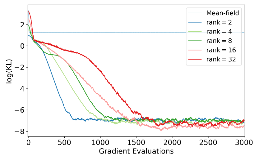
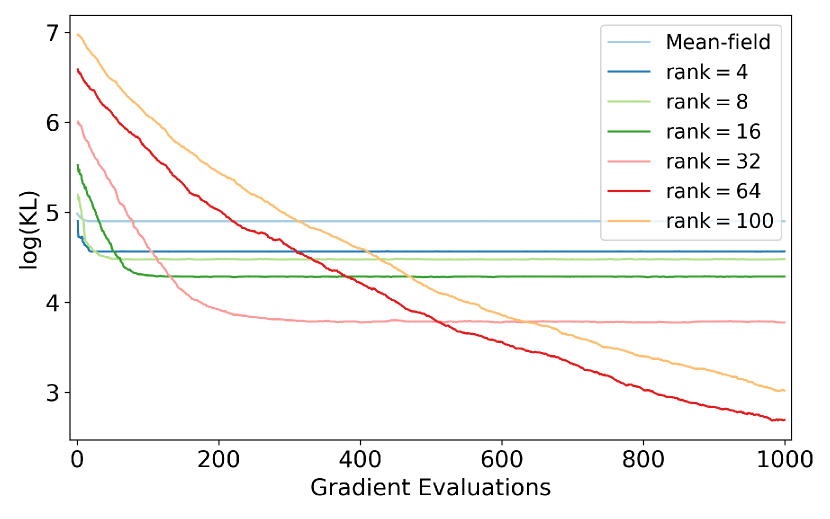
Figure 2: Significant computational benefits can be achieved with employing the low-rank Gaussian inferential model, while high ranks trade computational efficiency for statistical accuracy. Evolution of KL is compared across Gaussian inferential models of different ranks as well as the mean-field inferential model. Left: dimension $d=100$, true rank $p^{*}=2$. Right: dimension $d=100$, true rank $p^{*}=64$.

We first study the impact of low-rank Gaussian variational approximation on Gaussian posteriors. This task is akin to the setup in Theorems 1 and 2 that performs variational inference on Gaussian posteriors; it evaluates the quality of low-rank Gaussian approximation of posteriors.

Experimental setup.  We consider a setting where the true posterior is assumed to be centered multivariate Gaussian: $p(\theta\,|\,\mathbf{x})\sim\mathcal{N}(0,\left(\Omega^{*}\right)^{-1})$, with dimension $d=100$. We consider $\Omega^{*}=D+M^{*}$, where $D=\alpha^{*}\mathrm{I}_{d}$ and $M^{*}$ is a random symmetric positive semi-definite matrix. The goal is to find a variational approximation $q(\theta\,|\,\mathbf{x})\in\mathcal{Q}_{p}$ to $p(\theta\,|\,\mathbf{x})$. Specifically, two configurations are examined, one constrains the random matrix $M^{*}$ to be of rank $p^{*}=2$ and the other of rank $p^{*}=64$. In both cases, nonzero eigenvalues of $M^{*}$ are all bounded away from 0.

To illustrate the trade-offs in variational inference as in Theorems 1 and 2, we parameterize the precision matrix as $\Omega=\alpha\mathrm{I}_{d}+U\Lambda U^{\top}$ and restrict our variational family accordingly: $q=q_{(U,\Lambda)}$. We adopt our stochastic variational inference algorithm (Algorithm 1) and update the parameters $U,\Lambda$ in a sequential way. We first learn $U$ by setting $\Lambda$ to be $\mathrm{I}_{p}$, and use QR decomposition to ensure that $U$ is semi-orthonormal. In this experiment, we fix the number of stochastic gradient samples $N=1$ in Algorithm 1. We then determine $\Lambda$ with the optimized $U$. The training process continues until convergence of $\mathrm{KL}\left(q\leavevmode\nobreak\ \|\leavevmode\nobreak\ p\right)$ is achieved.

Results.  To empirically evaluate the statistical and computational trade-offs, we study the posterior inference error of variational inference under different inferential models, namely the KL divergence between the exact posterior and its variational approximation as in Theorem 1, including both the mean-field inferential model and the low-rank Gaussian one.

Figure 2 illustrates how the posterior inference error decreases over training epochs given Gaussian inferential models of different ranks. It shows that significant computational benefits can be achieved with low-rank approximation of the posteriors. By decreasing the rank of the inferential model, we achieve fast convergence within a small number of epochs (equivalently, a small number of gradient evaluations). However, the variational approximation accuracy degrades; the correlation structure of the posterior cannot be captured in fine granularity.

Figure 2 also shows that, when higher variational approximation accuracy is desired, we can increase the rank of the inferential model up to the true rank of $M^{*}$. When the rank of the inferential model is greater than or equal to the rank of the true model $M^{*}$, increasing rank would no longer improve accuracy but would notably increase the computational time.

Figure 3 demonstrates how variational approximation quality varies under different inferential models. By comparing the contours of the selected bivariate marginals of both the exact and approximate posteriors, we observe that variational approximation quality can be improved only up to when the true rank is reached. It also shows that the mean-field inferential model, though computationally efficient, tends to under-estimate the variance and correlation among different variables. Increasing the rank of the inferential model helps capture the posterior covariance.

6.2 Bayesian Logistic Regression

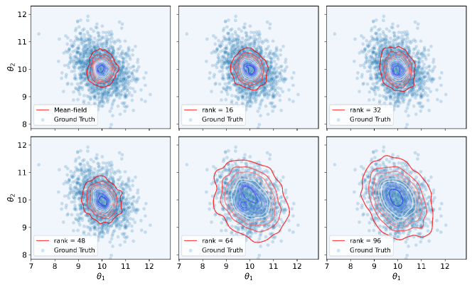
Figure 3: Gaussian inferential models with higher ranks lead to better approximation to the Gaussian posterior. The figure compares the bivariate marginals of the variational posterior with different ranks. True rank of the exact posterior is configured to be $p^{*}=64$ with dimension of data $d=100$. Each distribution contour graph results from $1500$ samples from the exact posterior and its variational approximation.

We next study variational inference in a Bayesian logistic regression task on a real dataset of cardiac arrhythmia in the patients. The goal of the logistic regression is to infer the probability of presence of cardiac arrhythmia in patients.

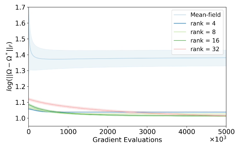
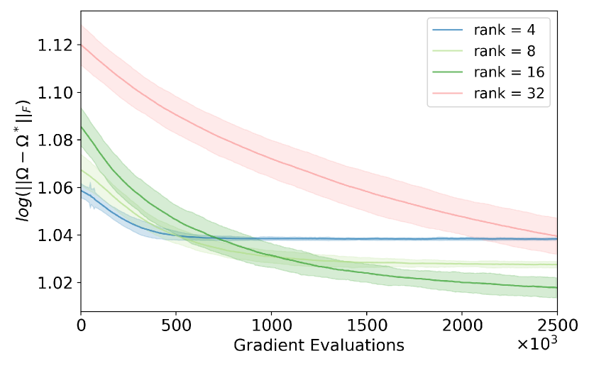
Figure 4: The optimal inferential model varies under different computational budget (e.g. the number of epochs) on the cardiac arrhythmia dataset (dimension d = 110). Left: Compared with low-rank inferential model, the mean-field inferential model converges to a higher posterior inference error; the convergence also exhibits higher variance. Right: Convergence of inferential models with rank $p=4,8,16,32$. Inferential models with lower ranks trade statistical accuracy for computational efficiency.

Experimental setup.  We first learn the mean parameter $\mu$ and then fix $\mu$ and learn $\mathcal{N}(\mu,\Omega^{-1})$ in the Gaussian inferential model $\mathcal{Q}_{p}$, which is the crux of the estimation problem and our focus. We also adopt a prior distribution of $\mathcal{N}(\mu,\beta\mathrm{I}_{d})$, with some positive constant $\beta$, over the logistic regression parameter $\theta$. Applying the low-rank variational inferencial model with the same parameterization as $\Omega^{(t)}=\alpha\mathrm{I}_{d}+U^{(t)}\Lambda\left(U^{(t)}\right)^{\top}$, we again run Algorithm 1 to sequentially optimize the learnable parameters: unitary matrix $U$ and diagonal matrix $\Lambda$. In this experiment, we fix the number of stochastic gradient samples $N=5000$ in Algorithm 1 due to the higher variance in samples of the gradient log posterior as compared to the Gaussian case.

To evaluate the effectiveness of the low-rank Gaussian inferential model in variational inference, we use a long run of the No-U-Turn Sampler (NUTS) (Hoffman and Gelman,, 2014) with multiple Markov chains to obtain a baseline estimate $\Omega^{*}$ of the posterior precision given the dataset. We evaluate the distance between the baseline $\Omega^{*}$ and the precision matrix $\Omega$ returned by variational approximation, via measuring the Frobenius norm difference $\left\|\Omega-\Omega^{*}\right\|_{F}$, for both the mean-field inferential model and the low-rank Gaussian model with rank $p=4,8,16,32$.

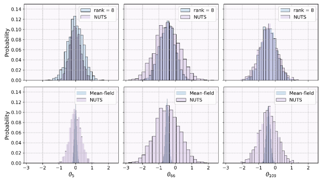
Figure 7: Low-rank variational approximation outperforms mean-field inferential model in terms of statistical accuracy. Comparison is performed against NUTS baseline given sufficient computational budget on the cardiac arrhythmia dataset (dimension d = 110). Marginal distributions are plotted for selected coordinates. Top: Low-rank inference model with rank $p=8$ against NUTS. Bottom: Mean-field model against NUTS.

Results.  Figure 4 compares the convergence behaviors of variational approximation under inferential models of different ranks. Similar to the earlier synthetic multivariate Gaussian experiment, we observe the statistical and computational trade-offs under different choices of inferential models. Specifically, the optimal inferential model varies under different computational budget (e.g. the number of epochs). Higher variance is also detected with increasing ranks of the inferential model. Moreover, low-rank Gaussian inferential models outperforms the mean-field inferential model in terms of posterior inference accuracy. The observed discrepancy in statistical accuracy is further demonstrated in Figures 7 and 8 in Section E.4. It compares the marginal distributions obtained by both variational families against the NUTS baseline, where low-rank variational model achieves significantly better approximation with higher accuracy.

Discussion

This paper initiates a theoretical study of the statistical and computational trade-offs arising in variational inference. Through a case study in inferential model selection, we establish this trade-off under the low-rank Gaussian inferential model. We prove that, as the rank of the inferential model increases, it can capture a larger subspace of the posterior uncertainty. Yet, this gain comes at the cost of slower convergence of the optimization algorithm. These results shed light on the practical success of low-rank approximations in Bayesian inference (Miller et al.,, 2017).

Supplementary Materials

Appendix A Details of Algorithms 2 and 3

Input: $\Omega$, $p$, $N$, $M$, $T$

Initialize $U^{(0)}=\left[e_{1},\dots,e_{p}\right]$, $\Lambda^{(0)}=\mathrm{I}_{p}$

for $t=0,\ldots,T-1$ do

      

$$\text{Sample i.i.d.}\;\theta_{j}^{(t)}\sim\mathcal{N}\left(0,\Omega^{-1}\right),\forall j\in\{1,\dots,N\},$$ (30)

$$\tilde{U}^{(t+1)}=\sum_{j=1}^{N}\left(\nabla\psi\left(\theta_{j}^{(t)}\right)\left(\theta_{j}^{(t)}\right)^{\top}\Omega\right)U^{(t)},$$ (31)

$$U^{(t+1)}=\mathrm{QR}\left(\widetilde{U}^{(t+1)}\right).$$ (32)

end for

Draw $\left\{\theta_{1},\dots,\theta_{M}\right\}$ i.i.d. from $\mathcal{N}\left(0,\Omega^{-1}\right)$

for $i=1,\dots,p$ do

      

$$\Lambda_{i,i}^{(T)}=\frac{1}{M}\sum_{j=1}^{M}\left(u_{i}^{(T)}\right)^{\top}\left(\frac{\nabla\psi(\theta_{j}+\Delta\cdot u_{i}^{(T)})-\nabla\psi(\theta_{j}-\Delta\cdot u_{i}^{(T)})}{2\Delta}\right)-D_{i,i}.$$ (33)

end for

Return: $U^{(T)},\Lambda^{(T)}$

Algorithm 2 SVI algorithm for Gaussian posterior (SVI_Gauss)

Input: $U_{0}=\left[e_{1},\dots,e_{p}\right]$, $\Lambda_{0}=\mathrm{I}_{p}$, $p$, $N$, $M$, $T$, $K$

for $k=0,\ldots,K-1$ do

      

$$\Omega_{k}=D+U_{k}\Lambda_{k}\left(U_{k}\right)^{\top}$$

$$\left(U_{k+1},\Lambda_{k+1}\right)=\textrm{SVI\_Gauss}\left(\Omega_{k},p,N,M,T\right).$$ (34)

end for

Return: $U_{K},\Lambda_{K}$

Algorithm 3 SVI algorithm for general posterior (SVI_General)

Appendix B Proofs for the Convergence of Stochastic Optimization over the KL Divergence

Proof of Theorem 1.

$$\mathrm{KL}\left(q_{\left(U^{(T)},\Lambda^{(T)}\right)}(\theta\,|\,\mathbf{x})\leavevmode\nobreak\ \|\leavevmode\nobreak\ p(\theta\,|\,{\bf x})\right) =\frac{1}{2}\left(\log\frac{|\Omega^{(T)}|}{|\Omega^{(\infty)}|}-d+\mathrm{tr}\left(\left(\Omega^{(T)}\right)^{-1}\Omega^{(\infty)}\right)\right)$$

$$=\frac{1}{2}\left(-\log\big{|}\left(\Omega^{(T)}\right)^{-1}\Omega^{(\infty)}\big{|}+\mathrm{tr}\left(\left(\Omega^{(T)}\right)^{-1}\Omega^{(\infty)}-\mathrm{I}\right)\right).$$

Since

$$\log\Big{|}\left(\Omega^{(T)}\right)^{-1}\Omega^{(\infty)}\Big{|}\geq\mathrm{tr}\left(\mathrm{I}-\left(\Omega^{(\infty)}\right)^{-1}\Omega^{(T)}\right),$$

$$\mathrm{KL}\left(q_{\left(U^{(T)},\Lambda^{(T)}\right)}(\theta\,|\,\mathbf{x})\leavevmode\nobreak\ \|\leavevmode\nobreak\ p(\theta\,|\,{\bf x})\right) \leq\frac{1}{2}\mathrm{tr}\left(\left(\Omega^{(T)}\right)^{-1}\Omega^{(\infty)}+\left(\Omega^{(\infty)}\right)^{-1}\Omega^{(T)}-2\mathrm{I}\right)$$

$$=\frac{1}{2}\mathrm{tr}\left(\left(\left(\Omega^{(T)}\right)^{-1}-\left(\Omega^{(\infty)}\right)^{-1}\right)\left(\Omega^{(\infty)}-\Omega^{(T)}\right)\right)$$

$$=\frac{1}{2}\mathrm{tr}\left(\left(\Omega^{(T)}\right)^{-1}\left(\Omega^{(\infty)}-\Omega^{(T)}\right)\left(\Omega^{(\infty)}\right)^{-1}\left(\Omega^{(\infty)}-\Omega^{(T)}\right)\right)$$

$$\leq\frac{1}{2}\sigma_{\max}\left(\left(\Omega^{(\infty)}\right)^{-1}\right)\sigma_{\max}\left(\left(\Omega^{(T)}\right)^{-1}\right)\cdot\left\|\Omega^{(\infty)}-\Omega^{(T)}\right\|_{F}^{2}$$

$$\leq\frac{1}{2\alpha^{2}}\left\|\Omega^{(\infty)}-\Omega^{(T)}\right\|_{F}^{2}.$$

We then bound $\left\|\Omega^{(\infty)}-\Omega^{(T)}\right\|_{F}^{2}$ in what follows. Since $\Omega^{(T)}$ and $\Omega^{(\infty)}$ share the same $D=\alpha\mathrm{I}_{d}$ matrix, we can define $M^{(T)}=\Omega^{(T)}-\alpha\mathrm{I}_{d}=U^{(T)}\Lambda^{(T)}\left(U^{(T)}\right)^{\top}$ and $M^{(\infty)}=\Omega^{(\infty)}-\alpha\mathrm{I}_{d}=U^{(\infty)}\Lambda^{(\infty)}\left(U^{(\infty)}\right)^{\top}$ and obtain:

$$\mathrm{tr}\left(\left(\Omega^{(\infty)}-\Omega^{(T)}\right)^{2}\right) =\mathrm{tr}\left(\left(\Lambda^{(T)}\right)^{2}\right)+\mathrm{tr}\left(\left(\Lambda^{(\infty)}\right)^{2}\right)-2\mathrm{tr}\left(\Lambda^{(T)}\left(U^{(T)}\right)^{\top}M^{(\infty)}U^{(T)}\right).$$ (35)

Since $\left(\left(U^{(T)}\right)^{\top}M^{(\infty)}U^{(T)}\right)_{i,j}=\left(u_{i}^{(T)}\right)^{\top}M^{(\infty)}u_{j}^{(T)}$, we have $\left(\Lambda^{(T)}\left(U^{(T)}\right)^{\top}M^{(\infty)}U^{(T)}\right)_{i,j}=\lambda_{i}^{(T)}\left(u_{i}^{(T)}\right)^{\top}M^{(\infty)}u_{j}^{(T)}$. Therefore,

$$\mathrm{tr}\left(\Lambda^{(T)}\left(U^{(T)}\right)^{\top}M^{(\infty)}U^{(T)}\right)=\sum_{k=1}^{p}\lambda_{k}^{(T)}\left(u_{k}^{(T)}\right)^{\top}M^{(\infty)}u_{k}^{(T)}.$$

From Proposition 1, we know that taking number of stochastic gradient samples per iteration $N=\widetilde{\boldsymbol{\Omega}}\left(\max\left\{\frac{pd}{m_{0}^{2}},\frac{p^{2}}{m_{0}^{4}}\right\}\cdot\frac{L^{4}}{\alpha^{2}}\cdot\frac{\kappa(\Omega)}{\epsilon^{2}\sqrt{\delta}}\right)$, and number of iterations $T=\boldsymbol{\Theta}\left(\frac{L}{\epsilon}\log\frac{1}{m_{0}}\right)$, we have with probability $1-\delta/2$:

$$\left(u^{(T)}_{k}\right)^{\top}M^{(\infty)}u^{(T)}_{k}\geq\lambda^{(\infty)}_{k}-2\epsilon,\qquad\forall k\in\{1,\dots,p\}.$$

Hence $\mathrm{tr}\left(\Lambda^{(T)}\left(U^{(T)}\right)^{\top}M^{(\infty)}U^{(T)}\right)\geq\sum_{k=1}^{p}\left(\lambda_{k}^{(T)}\lambda_{k}^{(\infty)}-2\epsilon\lambda^{(\infty)}_{k}\right)$. Therefore,

$$\mathrm{tr}\left(\left(\Omega^{(\infty)}-\Omega^{(T)}\right)^{2}\right)$$ (36)

$$=\sum_{k=1}^{p}\left(\lambda_{k}^{(T)}\right)^{2}+\sum_{k=1}^{d}\left(\lambda^{(\infty)}_{k}\right)^{2}-2\sum_{k=1}^{p}\lambda_{k}^{(T)}\left(u_{k}^{(T)}\right)^{\top}M^{(\infty)}u_{k}^{(T)}$$

$$=\sum_{k=p+1}^{d}\left(\lambda^{(\infty)}_{k}\right)^{2}+\sum_{k=1}^{p}\left(\lambda_{k}^{(T)}\right)^{2}+\sum_{k=1}^{p}\left(\lambda^{(\infty)}_{k}\right)^{2}-2\sum_{k=1}^{p}\lambda_{k}^{(T)}\left(u_{k}^{(T)}\right)^{\top}M^{(\infty)}u_{k}^{(T)}$$

$$\leq\sum_{k=p+1}^{d}\left(\lambda^{(\infty)}_{k}\right)^{2}+\sum_{k=1}^{p}\left(\lambda^{(\infty)}_{k}-\lambda_{k}^{(T)}\right)^{2}+4\epsilon\sum_{k=1}^{p}\lambda^{(\infty)}_{k}.$$ (37)

From Proposition 2, we know that when we take $n\geq 2p\log(8p/\delta)\cdot\frac{L^{2}}{\epsilon^{2}}$ and $\varDelta\leq\epsilon/\left(\sqrt{p}\cdot L_{\rm{Hess}}\right)$ in Algorithm 2 (Equation 33), we can achieve with $1-\delta/2$ probability that:

$$\sum_{k=1}^{p}\left(\lambda^{(\infty)}_{k}-\lambda^{(T)}_{k}\right)^{2}\leq 2\sum_{k=p+1}^{d}\left(\lambda^{(\infty)}_{k}\right)^{2}+8\epsilon\sum_{k=1}^{p}\lambda^{(\infty)}_{k}+8\epsilon^{2}.$$ (38)

Plugging equation (38) into (37), we arrive at the result that with $1-\delta$ probability,

$$\left\|\Omega^{(\infty)}-\Omega^{(T)}\right\|_{F}^{2}\leq 3\sum_{k=p+1}^{d}(\lambda^{(\infty)}_{k})^{2}+12\epsilon\sum_{k=1}^{p}\lambda_{k}^{(\infty)}+8\epsilon^{2}.$$

Therefore with $1-\delta$ probability,

$$\mathrm{KL}\left(q_{\left(U^{(T)},\Lambda^{(T)}\right)}(\theta\,|\,\mathbf{x})\leavevmode\nobreak\ \|\leavevmode\nobreak\ p(\theta\,|\,{\bf x})\right) \leq\frac{1}{2\alpha^{2}}\left\|\Omega^{(\infty)}-\Omega^{(T)}\right\|_{F}^{2}$$

$$\leq\frac{3}{2\alpha^{2}}\sum_{k=p+1}^{d}\left(\lambda^{(\infty)}_{k}\right)^{2}+\frac{6}{\alpha^{2}}\epsilon\sum_{k=1}^{p}\lambda^{(\infty)}_{k}+\frac{4\epsilon^{2}}{\alpha^{2}}.$$

Plugging in the computation budget of $\Pi=N\cdot T+2M=\widetilde{\boldsymbol{\Omega}}\left(pd\cdot\frac{L^{5}}{\alpha^{2}}\cdot\frac{1}{\epsilon^{3}\sqrt{\delta}}\right)$, we obtain that

$$\mathrm{KL}\left(q_{\left(U^{(T)},\Lambda^{(T)}\right)}(\theta\,|\,\mathbf{x})\leavevmode\nobreak\ \|\leavevmode\nobreak\ p(\theta\,|\,{\bf x})\right)\lesssim\frac{1}{\alpha^{2}}\sum_{k=p+1}^{d}\left(\lambda^{(\infty)}_{k}\right)^{2}+\left(\frac{pd}{\Pi}\right)^{1/3}\cdot\left(\frac{L}{\alpha}\right)^{5/3}\cdot\frac{1}{\delta^{1/6}}\cdot\frac{1}{\alpha}\sum_{k=1}^{p}\lambda^{(\infty)}_{k},$$

with $1-\delta$ probability. ∎

B.1 Proofs for solving for $U$

Proof of Lemma 2.

Taking $h_{t}=1$ and fixing $\Lambda=\mathrm{I}_{p}$ in the updates of equations (10)–(12), we have

$$\text{Sample i.i.d.}\;\theta_{j}^{(t)}\sim q_{\left(U^{(t)},\Lambda\right)},\forall j=\{1,\dots,N\}$$ (39)

$$\tilde{U}^{(t+1)}=\frac{1}{N}\sum_{j=1}^{N}\left(\nabla\psi\left(\theta_{j}^{(t)}\right)\theta_{j}^{\top}\right)U^{(t)}$$ (40)

$$U^{(t+1)}=\mathrm{QR}\left(\tilde{U}^{(t+1)}\right),$$ (41)

where $q_{\left(U^{(t)},\Lambda\right)}=\mathcal{N}\left(0,\left(\Omega^{(t)}\right)^{-1}\right)$, since $\Omega^{(t)}=D+U^{(t)}\Lambda\left(U^{(t)}\right)^{\top}$.

For $D=\alpha\mathrm{I}_{d}$, and for $\Lambda=\mathrm{I}_{p}$,

$$\Omega^{(t)}U^{(t)}=\left(D+U^{(t)}\Lambda\left(U^{(t)}\right)^{\top}\right)U^{(t)}=\left(\alpha\mathrm{I}_{d}+U^{(t)}\mathrm{I}_{p}\left(U^{(t)}\right)^{\top}\right)U^{(t)}=\left(\alpha+1\right)U^{(t)}.$$

Equation (40) becomes

$$\tilde{U}^{(t+1)}=\frac{1}{(\alpha+1)N}\sum_{j=1}^{N}\left(\nabla\psi\left(\theta_{j}^{(t)}\right)\theta_{j}^{\top}\right)\Omega^{(t)}U^{(t)}.$$

Combining with the fact that the QR decomposition will remove any scaling factor, we obtain the final result that the updates of equations (10)–(12) is equivalent to:

$$\text{Sample i.i.d.}\;\theta_{j}^{(t)}\sim\mathcal{N}\left(0,\left(\Omega^{(t)}\right)^{-1}\right),\forall j=\{1,\dots,N\}$$ (42)

$$\tilde{U}^{(t+1)}=\sum_{j=1}^{N}\left(\nabla\psi\left(\theta_{j}^{(t)}\right)\theta_{j}^{\top}\right)\Omega^{(t)}U^{(t)}$$ (43)

$$U^{(t+1)}=\mathrm{QR}\left(\tilde{U}^{(t+1)}\right),$$ (44)

where $\Omega^{(t)}=D+U^{(t)}\Lambda\left(U^{(t)}\right)^{{\top}}=\alpha\mathrm{I}_{d}+U^{(t)}\left(U^{(t)}\right)^{\top}$.

In addition, if the posterior is a normal distribution, then $\psi$ is a quadratic function and $\psi(\theta)=\frac{1}{2}\theta^{\top}\Omega^{(\infty)}\theta$. In that case, define stochastic update matrix $\widetilde{F}_{\psi}=\frac{1}{N}\sum_{i=1}^{N}\nabla\psi(\theta_{i})\theta_{i}^{\top}\Omega^{(t-1)}$. Then

$$F_{\psi}=\mathbb{E}[\widetilde{F}_{\psi}]=\mathbb{E}_{\theta\sim\mathcal{N}\left(0,\left(\Omega^{(t-1)}\right)^{-1}\right)}\left[\Omega^{(\infty)}\theta\theta^{\top}\Omega^{(t-1)}\right]=\Omega^{(\infty)}.$$

Substituting $\left(\Omega^{(t-1)}\right)$ with an arbitrary $\Omega$ yields the same result that

$$\mathbb{E}_{\theta\sim\mathcal{N}\left(0,\left(\Omega\right)^{-1}\right)}\left[\Omega^{(\infty)}\theta\theta^{\top}\Omega\right]=\Omega^{(\infty)}=F_{\psi}.$$

We can therefore apply the following update rule in the Gaussian posterior case:

$$\text{Sample i.i.d.}\;\theta_{j}^{(t)}\sim\mathcal{N}\left(0,\left(\Omega\right)^{-1}\right),\forall j=\{1,\dots,N\}$$ (45)

$$\tilde{U}^{(t+1)}=\sum_{j=1}^{N}\left(\nabla\psi\left(\theta_{j}^{(t)}\right)\theta_{j}^{\top}\right)\Omega\cdot U^{(t)}$$ (46)

$$U^{(t+1)}=\mathrm{QR}\left(\tilde{U}^{(t+1)}\right),$$ (47)

for any positive definite $\Omega$. ∎

Proof of Proposition 1.

When $p(\theta|{\bf x})$ is a normal distribution, $\nabla_{\theta}^{2}\psi(\theta)=\Omega^{(\infty)}$, and that $\nabla_{\theta}\psi(\theta)=\Omega^{(\infty)}\theta$, $\forall\theta\in\mathbb{R}^{d}$. Since $\psi$ is $\alpha$-strongly convex, we consider the following form:

$$\Omega^{(\infty)}=U^{(\infty)}\Lambda^{(\infty)}\left(U^{(\infty)}\right)^{\top}+\alpha\mathrm{I}_{d\times d}=U^{(\infty)}\left(\Lambda^{(\infty)}+\alpha\mathrm{I}_{d\times d}\right)\left(U^{(\infty)}\right)^{\top},$$

where $U^{(\infty)},\Lambda^{(\infty)}\in\mathbb{R}^{d\times d}$, and the eigenvalues $\lambda^{(\infty)}_{k}=\Lambda^{(\infty)}_{k,k}$ are non-negative and are ranked in a descending order.

We denote ${U}^{(\infty)}_{k}$ as the matrix consisting of the top $k$ eigenvectors of $\Omega^{(\infty)}$. Conversely, denote $U^{(\infty)}_{-k}$ as the matrix consisting of the bottom $(d-k)$ eigenvectors of $\Omega^{(\infty)}$ and similarly ${U}^{(\infty)}_{-k-\iota(\epsilon)}$ as the matrix consisting of all eigenvectors of $\Omega^{(\infty)}$ with eigenvalues less than or equal to $\lambda^{(\infty)}_{k}+\alpha-\epsilon$ (assuming there are $(d-k-\iota(\epsilon))$ of them). For $U^{(t)}\in\mathbb{R}^{p\times p}$, we similarly denote for $k\leq p$: $U^{(t)}_{k}=\left[u^{(t)}_{1},\dots,u^{(t)}_{k}\right]$ as the matrix consisting of the first $k$-columns of $U^{(t)}$.

We now leverage the following Proposition 3 to bound the Rayleigh quotient $\left(u^{(T)}_{k}\right)^{\top}\Omega^{(\infty)}u^{(T)}_{k}$.

We apply Proposition 3 and similarly let $m_{0}=\sigma_{\min}\left((U^{(\infty)}_{p})^{\top}U^{(0)}\right)\geq\max\left(0,1-\left\|U^{(\infty)}_{p}-U^{(0)}\right\|\right)$ to prove the lemma. We run the stochastic variational inference algorithm for Gaussian posterior described in equations (14) to (16) with input matrix $\Omega$, number of stochastic gradient samples per iteration $N=\widetilde{\boldsymbol{\Omega}}\left(\max\left\{\frac{pd}{m_{0}^{2}},\frac{p^{2}}{m_{0}^{4}}\right\}\cdot\frac{L^{4}}{\alpha^{2}}\cdot\frac{\kappa(\Omega)}{\epsilon^{2}\sqrt{\delta}}\right)$, and number of iterations $T=\Theta\left(\frac{L}{\epsilon}\log\frac{1}{m_{0}}\right)$. We obtain that with probability $1-\delta$, for all $m\geq k$, for any $k\leq p$,

$$\left\|\left({U}^{(\infty)}_{-m-1}\right)^{\top}U_{k}^{(T)}\right\|\leq\frac{\epsilon}{\lambda_{k}^{(\infty)}-\lambda_{m+1}^{(\infty)}},$$

which implies that with probability $1-\delta$,

$$\forall k\in\{1,\dots,p\},\ \forall\gamma_{k,i}=\frac{\lambda_{k}^{(\infty)}-\lambda_{i}^{(\infty)}}{\epsilon}\geq 1,\qquad\left\|\left({U}^{(\infty)}_{-k-\iota(\gamma\cdot\epsilon)}\right)^{\top}u^{(t)}_{k}\right\|_{2}^{2}\leq 1/\gamma_{k,i}^{2}.$$ (48)

We use the above result to bound the Rayleigh quotient for $\Omega^{(\infty)}=U^{(\infty)}\left({\Lambda}^{(\infty)}+\alpha\mathrm{I}_{d\times d}\right)\left({U}^{(\infty)}\right)^{\top}$. For each $k\in[p]$, denote $k_{0}=k+\iota(\epsilon)$. Then $(k_{0}+1)$ indexes the first eigenvector with eigenvalue less than or equal to $\lambda^{(\infty)}_{k}+\alpha-\epsilon$. Define $b_{k,j}=\sum_{s=j}^{d}\left\langle u^{(t)}_{k},u^{(\infty)}_{s}\right\rangle^{2}$ where $u^{(\infty)}_{s}$ is the $s$-th eigenvector of $\Omega^{(\infty)}$. It satisfies $b_{k,1}=\left(u^{(t)}_{k}\right)^{\top}\left(\sum_{s=1}^{d}u^{(\infty)}_{s}\left(u^{(\infty)}_{s}\right)^{\top}\right)u^{(t)}_{k}=1$. By Abel’s transformation,

$$\left(u^{(t)}_{k}\right)^{\top}\Omega^{(\infty)}u^{(t)}_{k} =\sum_{j=1}^{d}\left(\lambda^{(\infty)}_{j}+\alpha\right)\left\langle u^{(t)}_{k},u^{(\infty)}_{j}\right\rangle^{2}$$

$$=\sum_{j=1}^{k_{0}-1}\left(\lambda^{(\infty)}_{j}+\alpha\right)\left\langle u^{(t)}_{k},u^{(\infty)}_{j}\right\rangle^{2}+\left(\lambda^{(\infty)}_{k_{0}}+\alpha\right)b_{k,k_{0}}-\sum_{j=k_{0}+1}^{d}b_{k,j}\left(\lambda^{(\infty)}_{j-1}-\lambda^{(\infty)}_{j}\right)$$

$$\geq(\lambda^{(\infty)}_{k}+\alpha-\epsilon)b_{k,1}-\sum_{j=k_{0}+1}^{d}b_{k,j}\left(\lambda^{(\infty)}_{j-1}-\lambda^{(\infty)}_{j}\right)$$

$$=(\lambda^{(\infty)}_{k}+\alpha-\epsilon)-\sum_{j=k_{0}+1}^{d}b_{k,j}\left(\lambda^{(\infty)}_{j-1}-\lambda^{(\infty)}_{j}\right).$$ (49)

According to equation (48), for every $i\geq k_{0}+1$, $b_{k,j}=\left\|{U}^{(\infty)}_{-k-\iota(\gamma_{k,j}\cdot\epsilon)}u^{(t)}_{k}\right\|_{2}^{2}\leq\frac{1}{\gamma_{k,j}^{2}}$. Plugging this result into equation (49), we obtain

$$\sum_{j=k_{0}+1}^{d}b_{k,j}\left(\lambda^{(\infty)}_{j-1}-\lambda^{(\infty)}_{j}\right)\leq\sum_{j=k_{0}+1}^{d}\frac{1}{\gamma_{k,j}^{2}}\epsilon\left(\gamma_{k,j}-\gamma_{k,j-1}\right)\leq\epsilon\int_{1}^{1/\epsilon}\frac{1}{\gamma^{2}}d\gamma\leq\epsilon.$$

Therefore, with probability $1-\delta$,

$$\left(u^{(t)}_{k}\right)^{\top}\Omega^{(\infty)}u^{(t)}_{k}\geq\lambda^{(\infty)}_{k}+\alpha-2\epsilon.$$

∎

Proposition 3.

Assume that function $\psi(\theta)=\frac{1}{2}\theta^{\top}\Omega^{(\infty)}\theta$ (so that the posterior $p(\theta|{\bf x})$ is Gaussian) and is $\alpha$-strongly convex and $L$-Lipschitz smooth.We denote the initial condition: $m_{0}=\sigma_{\min}\left((U^{(\infty)}_{p})^{\top}U^{(0)}\right)\geq\max\left(0,1-\left\|U^{(\infty)}_{p}-U^{(0)}\right\|\right)$. We run the stochastic variational inference algorithm for Gaussian posterior described in equations (14) to (16) with input matrix $\Omega$, number of stochastic gradient samples per iteration, and number of iterations:

$$N =\widetilde{\Omega}\left(\max\left\{\frac{pd}{m_{0}^{2}},\frac{p^{2}}{m_{0}^{4}}\right\}\cdot\frac{L^{4}}{\alpha^{2}}\cdot\frac{\kappa(\Omega)}{\epsilon^{2}\sqrt{\delta}}\right),$$

$$T =\Theta\left(\frac{L}{\epsilon}\log\frac{1}{m_{0}}\right),$$

where $\epsilon\leq\lambda_{k}$. Then with probability $1-\delta$,

$$\left\|\left(U^{(\infty)}_{-m-1}\right)^{\top}U_{k}^{(T)}\right\|\leq\frac{\epsilon}{\lambda_{k}^{(\infty)}-\lambda_{m+1}^{(\infty)}},$$

for all $m\geq k$, for any $k\leq p$.

Proof of Proposition 3.

We now provide the proof of Proposition 3. For succinctness, we denote in this section $V_{k}={U}^{(\infty)}_{k}$; $W_{m}={U}^{(\infty)}_{-m-1}$; and the stochastic gradient noise restricted to the first $k$ columns:

$${G_{k}^{(t)}}=\frac{1}{N}\sum_{j=1}^{N}\nabla\psi(\theta_{j})\theta_{j}^{\top}\Omega{U_{k}^{(t)}}-\mathbb{E}_{\theta\sim\mathcal{N}\left(0,\Omega^{-1}\right)}\left[\nabla\psi(\theta)\theta^{\top}\Omega{U_{k}^{(t)}}\right].$$

We first state the following main lemma that will help us bound our objective via contraction.

Lemma 3.

Assume that $\left\|{G_{k}^{(t)}}\right\|\leq\Delta_{1}\cdot\lambda_{k}^{(\infty)}\cdot\sigma_{\min}\left(V_{k}^{\top}{U_{k}^{(t)}}\right)$ and $\left\|V_{k}^{\top}{G_{k}^{(t)}}\right\|\leq\Delta_{2}\cdot\lambda_{k}^{(\infty)}\cdot\sigma^{2}_{\min}\left(V_{k}^{\top}{U_{k}^{(t)}}\right)$, where $\Delta_{2}\leq 1/3$. Then for $h_{t}=\left\|W_{m}^{\top}{U_{k}^{(t)}}\left(V_{k}^{\top}{U_{k}^{(t)}}\right)^{+}\right\|$,

$$h_{t+1}-\frac{6\lambda_{k}^{(\infty)}\Delta_{1}+15\lambda_{m+1}^{(\infty)}\Delta_{2}}{\lambda_{k}^{(\infty)}-\lambda_{m+1}^{(\infty)}}\leq\frac{\lambda_{m+1}^{(\infty)}}{\lambda_{k}^{(\infty)}}\left(h_{t}-\frac{6\lambda_{k}^{(\infty)}\Delta_{1}+15\lambda_{m+1}^{(\infty)}\Delta_{2}}{\lambda_{k}^{(\infty)}-\lambda_{m+1}^{(\infty)}}\right).$$

Expanding the recursion, we obtain that

$$h_{t}\leq\left(\frac{\lambda_{m+1}^{(\infty)}}{\lambda_{k}^{(\infty)}}\right)^{t}h_{0}+\frac{6\lambda_{k}^{(\infty)}\Delta_{1}+15\lambda_{m+1}^{(\infty)}\Delta_{2}}{\lambda_{k}^{(\infty)}-\lambda_{m+1}^{(\infty)}}.$$

We now develop the conditions that will satisfy the premise of Lemma 3 with a uniform bound on $\sigma_{\min}\left(V_{k}^{\top}{U_{k}^{(t)}}\right)$ by the initial condition.

Lemma 4.

For $\left\|{G_{k}^{(t)}}\right\|\leq\eta\lambda_{k}^{(\infty)}$ and for $\left\|V_{k}^{\top}{G_{k}^{(t)}}\right\|\leq\frac{1}{10}\eta\lambda_{k}^{(\infty)}\cdot\sigma_{\min}\left(V_{k}^{\top}{U_{k}^{(t)}}\right)$,

$$\sigma_{\min}\left(V_{k}^{\top}{U_{k}^{(t)}}\right)\geq\frac{1}{6}\sigma_{\min}\left(V_{k}^{\top}U_{k}^{(0)}\right),$$

for all $t\leq 1/\eta$.

Applying this to Lemma 3, we achieve the result that when $\Delta_{1}=\mathcal{O}\left(\frac{\epsilon}{L}\right)$ and $\Delta_{2}=\mathcal{O}\left(\frac{\epsilon}{L}\right)$, and when $T=\Theta\left(\frac{L}{\epsilon}\log\frac{1}{\sigma_{\min}\left(V_{k}^{\top}U_{k}^{(0)}\right)}\right)$,

$$\left\|W_{m}^{\top}U_{k}^{(T)}\right\|\leq\frac{h_{T}}{\sigma_{\min}\left(V_{k}^{\top}U_{k}^{(T)}\right)}\leq\frac{\epsilon}{\lambda_{k}^{(\infty)}-\lambda_{m+1}^{(\infty)}},$$

with $W_{m}={U}^{(\infty)}_{-m-1}$, for any $m\geq k$. This leads to the requirement that for $\epsilon\leq\lambda_{k}^{(\infty)}$,

$$\left\|{G_{k}^{(t)}}\right\|=\mathcal{O}\left(\epsilon\cdot\frac{\alpha}{L}\cdot\sigma_{\min}\left(V_{k}^{\top}U_{k}^{(0)}\right)\right),\qquad\left\|V_{k}^{\top}{G_{k}^{(t)}}\right\|=\mathcal{O}\left(\epsilon\cdot\frac{\alpha}{L}\cdot\sigma_{\min}^{2}\left(V_{k}^{\top}U_{k}^{(0)}\right)\right),$$ (50)

since $\lambda_{k}^{(\infty)}\geq\alpha$, $\forall k$.

We then bound the stochastic gradient noise ${G_{k}^{(t)}}$ to fulfill this requirement.

Lemma 5.

For $\theta_{j}^{(t)}\sim\mathcal{N}\big{(}0,\Omega^{-1}\big{)}$, and for orthogonal matrix $V_{k}\in^{d\times k}$, the following bounds hold for $L$-Lipschitz smooth function $\psi$ with probability $1-\mathcal{O}\left(1/N^{2}\right)$, for any $k\leq p$:

$$\left\|{G_{k}^{(t)}}\right\|\lesssim L\sqrt{\kappa(\Omega)}\cdot\sqrt{\frac{pd\log^{4}(N)\log(d)}{N}}+L\sqrt{\kappa(\Omega)}\cdot\frac{\sqrt{pd}}{N^{2}},$$

and

$$\left\|V_{k}^{\top}{G_{k}^{(t)}}\right\|\lesssim L\sqrt{\kappa(\Omega)}\cdot\sqrt{\frac{p^{2}\log^{4}(N)\log(d)}{N}}+L\sqrt{\kappa(\Omega)}\cdot\frac{p}{N^{2}},$$

for any $k\leq p$. Here $\kappa(\Omega)=\sigma_{\max}(\Omega)/\sigma_{\min}(\Omega)$ is the condition number of the positive definite input matrix $\Omega$.

Applying Lemma 5 to the requirements in (50), we establish that when

$$N=\widetilde{\Omega}\left(\max\left\{\frac{pd}{\sigma_{\min}^{2}\left(V_{k}^{\top}U_{k}^{(0)}\right)},\frac{p^{2}}{\sigma_{\min}^{4}\left(V_{k}^{\top}U_{k}^{(0)}\right)}\right\}\cdot\frac{L^{4}}{\alpha^{2}}\cdot\frac{\kappa(\Omega)}{\epsilon^{2}\sqrt{\delta}}\right),$$

and when $T=\Theta\left(\frac{L}{\epsilon}\log\frac{1}{\sigma_{\min}\left(V_{k}^{\top}U_{k}^{(0)}\right)}\right)$, the following holds with probability $1-\delta$ for any $k\leq p$:

$$\left\|\left({U}^{(\infty)}_{-m-1}\right)^{\top}U_{k}^{(T)}\right\|=\left\|W_{m}^{\top}U_{k}^{(T)}\right\|\leq\frac{\epsilon}{\lambda_{k}^{(\infty)}-\lambda_{m+1}^{(\infty)}}.$$

Plugging in the following Weyl’s inequality for the initial condition yields the final result

$$1-\sigma_{\min}\left(V_{k}^{\top}U_{k}^{(0)}\right)\leq 1-\sigma_{\min}\left((U^{(\infty)}_{p})^{\top}U^{(0)}\right)\leq\left\|\mathrm{I}-\left(U^{(\infty)}_{p}\right)^{\top}U^{(0)}\right\|\leq\left\|U^{(\infty)}_{p}-U^{(0)}\right\|.$$

∎

B.1.1 Supporting Proofs

Proof of Lemma 3.

We first note that the update of the lower ranked ${U_{k}^{(t)}}$ is the same as the update of $U^{(t)}$ in equations (31) and (32) because of the properties of matrix multiplication and QR factorization. Writing ${\Omega^{(\infty)}}=\mathbb{E}_{\theta\sim\mathcal{N}\left(0,\Omega^{-1}\right)}\left[\nabla\psi(\theta)\theta^{\top}\Omega\right]$, the update rule for ${U_{k}^{(t)}}$ can be expressed as the mean update plus stochastic noise: $\widetilde{U}_{k}^{(t+1)}={\Omega^{(\infty)}}\cdot{U_{k}^{(t)}}+{G_{k}^{(t)}}$, ${U_{k}^{(t+1)}}=\mathrm{QR}\left(\widetilde{U}_{k}^{(t+1)}\right)$.

We then use this update rule to develop our object $W_{m}^{\top}{U_{k}^{(t+1)}}\left(V_{k}^{\top}{U_{k}^{(t+1)}}\right)^{+}$, where we define the pseudo-inverse: $Z^{+}=Z^{\top}\left(ZZ^{\top}\right)^{-1}$. Under this definition,

$$V_{k}^{\top}\left({\Omega^{(\infty)}}\cdot{U_{k}^{(t)}}+{G_{k}^{(t)}}\right)\left(R^{(t+1)}\right)^{-1}R^{(t+1)}\left(V_{k}^{\top}\left({\Omega^{(\infty)}}\cdot{U_{k}^{(t)}}+{G_{k}^{(t)}}\right)\right)^{+}=\mathrm{I}.$$

Hence

$$\left(V_{k}^{\top}{U_{k}^{(t+1)}}\right)^{+}=\left(V_{k}^{\top}\left({\Omega^{(\infty)}}\cdot{U_{k}^{(t)}}+{G_{k}^{(t)}}\right)\left(R^{(t+1)}\right)^{-1}\right)^{+}=R^{(t+1)}\left(V_{k}^{\top}\left({\Omega^{(\infty)}}\cdot{U_{k}^{(t)}}+{G_{k}^{(t)}}\right)\right)^{+}.$$

Expanding $W_{m}^{\top}{U_{k}^{(t+1)}}\left(V_{k}^{\top}{U_{k}^{(t+1)}}\right)^{+}$ using this result, we obtain that

$$W_{m}^{\top}{U_{k}^{(t+1)}}\left(V_{k}^{\top}{U_{k}^{(t+1)}}\right)^{+}=\left(\Lambda_{-m}^{(\infty)}W_{m}^{\top}{U_{k}^{(t)}}+W_{m}^{\top}{G_{k}^{(t)}}\right)\left(V_{k}^{\top}{U_{k}^{(t)}}+(\Lambda_{k}^{(\infty)})^{-1}V_{k}^{\top}{G_{k}^{(t)}}\right)^{+}(\Lambda_{k}^{(\infty)})^{-1}.$$

Denote ${Z^{(t)}}=V_{k}^{\top}{U_{k}^{(t)}}+(\Lambda_{k}^{(\infty)})^{-1}V_{k}^{\top}{G_{k}^{(t)}}$. Then we can upper bound $h_{t+1}$ as follows.

$$h_{t+1} =\left\|\left(\Lambda_{-m}^{(\infty)}W_{m}^{\top}{U_{k}^{(t)}}+W_{m}^{\top}{G_{k}^{(t)}}\right)\left({Z^{(t)}}\right)^{+}(\Lambda_{k}^{(\infty)})^{-1}\right\|$$

$$\leq\underbrace{\left\|\Lambda_{-m}^{(\infty)}W_{m}^{\top}{U_{k}^{(t)}}\left({Z^{(t)}}\right)^{+}(\Lambda_{k}^{(\infty)})^{-1}\right\|}_{T_{1}}+\underbrace{\left\|W_{m}^{\top}{G_{k}^{(t)}}\left({Z^{(t)}}\right)^{+}(\Lambda_{k}^{(\infty)})^{-1}\right\|}_{T_{2}}.$$

For the pseudo-inverse, $\left({Z^{(t)}}\right)^{+}=\left({Z^{(t)}}\right)^{\top}\left({Z^{(t)}}\left({Z^{(t)}}\right)^{\top}\right)^{-1}$, we use the Woodbury formula and develop its inverse part as follows:

$$\left({Z^{(t)}}\left({Z^{(t)}}\right)^{\top}\right)^{-1}={\widetilde{P}}^{-{\top}}\left(\mathrm{I}-\left(\mathrm{I}+Y\right)^{-1}Y\right){\widetilde{P}}^{-1},$$ (51)

where ${\widetilde{P}}\widetilde{V}^{\top}=V_{k}^{\top}{U_{k}^{(t)}}$ for a unitary matrix $\widetilde{V}$, and

$$Y=\widetilde{V}^{\top}{G_{k}^{(t)}}^{\top}V_{k}(\Lambda_{k}^{(\infty)})^{-1}{\widetilde{P}}^{-{\top}}+{\widetilde{P}}^{-1}(\Lambda_{k}^{(\infty)})^{-1}V_{k}^{\top}{G_{k}^{(t)}}\widetilde{V}+\widetilde{P}^{-1}(\Lambda_{k}^{(\infty)})^{-1}V_{k}^{\top}{G_{k}^{(t)}}{G_{k}^{(t)}}^{\top}V_{k}(\Lambda_{k}^{(\infty)})^{-1}{\widetilde{P}}^{-{\top}},$$

as defined in equation (52) in 1. 1 will also provide a bound on $\left\|\left(\mathrm{I}+Y\right)^{-1}Y\right\|$.

We now use equation (51) and the definition of ${Z^{(t)}}$ to expand term $T_{1}$. Since we have $\left({U_{k}^{(t)}}\right)^{\top}V_{k}\widetilde{P}^{-{\top}}\widetilde{P}^{-1}=\left(V_{k}^{\top}{U_{k}^{(t)}}\right)^{+}$ and $\left({U_{k}^{(t)}}\right)^{\top}V_{k}\widetilde{P}^{-{\top}}=\widetilde{V}$, we obtain that

$$T_{1} \leq\left\|\Lambda_{-m}^{(\infty)}W_{m}^{\top}{U_{k}^{(t)}}\left(\left(V_{k}^{\top}{U_{k}^{(t)}}\right)^{+}+\left({G_{k}^{(t)}}\right)^{\top}V_{k}(\Lambda_{k}^{(\infty)})^{-1}\widetilde{P}^{-{\top}}\widetilde{P}^{-1}\right)(\Lambda_{k}^{(\infty)})^{-1}\right\|$$

$$+\left\|\Lambda_{-m}^{(\infty)}W_{m}^{\top}{U_{k}^{(t)}}\left(\widetilde{V}\left(\mathrm{I}+Y\right)^{-1}Y\widetilde{P}^{-1}+\left({G_{k}^{(t)}}\right)^{\top}V_{k}(\Lambda_{k}^{(\infty)})^{-1}\widetilde{P}^{-{\top}}\left(\mathrm{I}+Y\right)^{-1}Y\widetilde{P}^{-1}\right)(\Lambda_{k}^{(\infty)})^{-1}\right\|$$

$$\stackrel{{\scriptstyle{\sf(i)}}}{{\leq}}\frac{\lambda_{m+1}^{(\infty)}}{\lambda_{k}^{(\infty)}}\left(h_{t}+\Delta_{2}+\frac{\frac{7}{3}\Delta_{2}}{1-\frac{7}{3}\Delta_{2}}+\frac{\frac{7}{3}\Delta_{2}^{2}}{1-\frac{7}{3}\Delta_{2}}\right)\leq\frac{\lambda_{m+1}^{(\infty)}}{\lambda_{k}^{(\infty)}}\left(h_{t}+15\Delta_{2}\right),$$

where ${\sf(i)}$ follows from 1. Similarly, by the bound on $\left\|{G_{k}^{(t)}}\right\|$ and 1,

$$T_{2} \leq\left\|W_{m}^{\top}{G_{k}^{(t)}}\left(\left(V_{k}^{\top}{U_{k}^{(t)}}\right)^{+}+\left({G_{k}^{(t)}}\right)^{\top}V_{k}(\Lambda_{k}^{(\infty)})^{-1}{\widetilde{P}}^{-{\top}}{\widetilde{P}}^{-1}\right)(\Lambda_{k}^{(\infty)})^{-1}\right\|$$

$$+\left\|W_{m}^{\top}{G_{k}^{(t)}}\left(\widetilde{V}(\mathrm{I}+Y)^{-1}Y{\widetilde{P}}^{-1}+\left({G_{k}^{(t)}}\right)^{\top}V_{k}(\Lambda_{k}^{(\infty)})^{-1}{\widetilde{P}}^{-{\top}}(\mathrm{I}+Y)^{-1}Y{\widetilde{P}}^{-1}\right)(\Lambda_{k}^{(\infty)})^{-1}\right\|$$

$$\leq\Delta_{1}+\Delta_{1}\Delta_{2}+\Delta_{1}\cdot\frac{\frac{7}{3}\Delta_{2}}{1-\frac{7}{3}\Delta_{2}}+\Delta_{1}\cdot\Delta_{2}\cdot\frac{\frac{7}{3}\Delta_{2}}{1-\frac{7}{3}\Delta_{2}}\leq 6\Delta_{1}.$$

Combining the two bounds, we arrive at our result that

$$h_{t+1}\leq\frac{\lambda_{m+1}^{(\infty)}}{\lambda_{k}^{(\infty)}}h_{t}+\left(15\frac{\lambda_{m+1}^{(\infty)}}{\lambda_{k}^{(\infty)}}\Delta_{2}+6\Delta_{1}\right).$$

Rearranging the terms yields the final expression. ∎

Fact 1.

Define

$$Y=\widetilde{V}^{\top}\left({G_{k}^{(t)}}\right)^{\top}V_{k}(\Lambda_{k}^{(\infty)})^{-1}{\widetilde{P}}^{-{\top}}+{\widetilde{P}}^{-1}(\Lambda_{k}^{(\infty)})^{-1}V_{k}^{\top}{G_{k}^{(t)}}\widetilde{V}\\ +\widetilde{P}^{-1}(\Lambda_{k}^{(\infty)})^{-1}V_{k}^{\top}{G_{k}^{(t)}}\left({G_{k}^{(t)}}\right)^{\top}V_{k}(\Lambda_{k}^{(\infty)})^{-1}{\widetilde{P}}^{-{\top}},$$ (52)

for a unitary matrix $\widetilde{V}\in^{d\times d}$, for $\Lambda_{k}^{(\infty)}$ containing eigenvalues bigger than or equal to $\lambda_{k}^{(\infty)}$, and for ${\widetilde{P}}\widetilde{V}^{\top}=V_{k}^{\top}{U_{k}^{(t)}}$. Then when $\left\|V_{k}^{\top}{G_{k}^{(t)}}\right\|\leq\Delta_{2}\cdot\lambda_{k}^{(\infty)}\cdot\sigma^{2}_{\min}\left(V_{k}^{\top}{U_{k}^{(t)}}\right)$ for $\Delta_{2}\leq 1/3$,

$$\left\|\left({G_{k}^{(t)}}\right)^{\top}V_{k}(\Lambda_{k}^{(\infty)})^{-1}{\widetilde{P}}^{-{\top}}\right\|\leq\Delta_{2}\cdot\sigma_{\min}\left(V_{k}^{\top}{U_{k}^{(t)}}\right),$$

and that

$$\left\|\left(\mathrm{I}+Y\right)^{-1}Y\right\|\leq\frac{\frac{7}{3}\Delta_{2}}{1-\frac{7}{3}\Delta_{2}}\cdot\sigma_{\min}\left(V_{k}^{\top}{U_{k}^{(t)}}\right).$$

Proof.

First note that for ${\widetilde{P}}\widetilde{V}^{\top}=V_{k}^{\top}{U_{k}^{(t)}}$, $\|{\widetilde{P}}^{-1}\|_{2}\leq 1/\sigma_{\min}\left(V_{k}^{\top}{U_{k}^{(t)}}\right)$. Then

$$\left\|\left({G_{k}^{(t)}}\right)^{\top}V_{k}(\Lambda_{k}^{(\infty)})^{-1}{\widetilde{P}}^{-{\top}}\right\|\leq\left\|V_{k}^{\top}{G_{k}^{(t)}}\right\|\cdot\left\|(\Lambda_{k}^{(\infty)})^{-1}\right\|_{2}\cdot\left\|{\widetilde{P}}^{-1}\right\|_{2}.$$

Plugging in the assumption yields the bound.

Similarly,

$$\left\|{\widetilde{P}}^{-1}(\Lambda_{k}^{(\infty)})^{-1}V_{k}^{\top}{G_{k}^{(t)}}\widetilde{V}\right\|\leq\left\|V_{k}^{\top}{G_{k}^{(t)}}\right\|\cdot\left\|(\Lambda_{k}^{(\infty)})^{-1}\right\|_{2}\cdot\left\|{\widetilde{P}}^{-1}\right\|_{2}\leq\Delta_{2}\cdot\sigma_{\min}\left(V_{k}^{\top}{U_{k}^{(t)}}\right),$$

and

$$\left\|\widetilde{P}^{-1}(\Lambda_{k}^{(\infty)})^{-1}V_{k}^{\top}{G_{k}^{(t)}}\left({G_{k}^{(t)}}\right)^{\top}V_{k}(\Lambda_{k}^{(\infty)})^{-1}{\widetilde{P}}^{-{\top}}\right\| \leq\left\|V_{k}^{\top}{G_{k}^{(t)}}\right\|^{2}\cdot\left\|(\Lambda_{k}^{(\infty)})^{-1}\right\|_{2}^{2}\cdot\left\|{\widetilde{P}}^{-1}\right\|_{2}^{2}$$

$$\leq\Delta_{2}^{2}\cdot\sigma^{2}_{\min}\left(V_{k}^{\top}{U_{k}^{(t)}}\right)\leq\frac{1}{3}\Delta_{2}\cdot\sigma_{\min}\left(V_{k}^{\top}{U_{k}^{(t)}}\right).$$

Combining the three terms, we obtain that

$$\left\|Y\right\|\leq\frac{7}{3}\Delta_{2}\cdot\sigma_{\min}\left(V_{k}^{\top}{U_{k}^{(t)}}\right),$$

and that

$$\left\|(\mathrm{I}+Y)^{-1}Y\right\|\leq\frac{\left\|Y\right\|}{1-\left\|Y\right\|_{2}}\leq\frac{\frac{7}{3}\Delta_{2}}{1-\frac{7}{3}\Delta_{2}}\cdot\sigma_{\min}\left(V_{k}^{\top}{U_{k}^{(t)}}\right).$$

∎

Proof of Lemma 4.

Following hardt2014, we can write $\cos\theta_{k}(V_{k},{U_{k}^{(t)}})=\sigma_{\min}\left(V_{k}^{\top}{U_{k}^{(t)}}\right)$ and $\tan\theta_{k}(V_{k},{U_{k}^{(t)}})=\left\|\left(V_{k}^{\bot}\right)^{\top}{U_{k}^{(t)}}\left(V_{k}^{\top}{U_{k}^{(t)}}\right)^{+}\right\|$, for $V_{k}^{\bot}=\bar{U}^{*}_{-k-1}$. From Lemma A.5 of Balcan2016, we know that for $\left\|{G_{k}^{(t)}}\right\|\leq c_{1}\eta\lambda_{k}^{(\infty)}$ and for $\left\|V_{k}^{\top}{G_{k}^{(t)}}\right\|\leq c_{2}\eta\lambda_{k}^{(\infty)}\cdot\sigma_{\min}\left(V_{k}^{\top}{U_{k}^{(t)}}\right)$, for all $t=0,1,\dots,T$,

$$\tan\theta_{k}(V_{k},{U_{k}^{(t)}})+\frac{c_{1}}{c_{1}+c_{2}} \leq\left(\frac{1+c_{1}\eta}{1-c_{2}\eta}\right)^{t}\left(\tan\theta_{k}(V_{k},U_{k}^{(0)})+\frac{c_{1}}{c_{1}+c_{2}}\right)$$

$$\leq\exp\left(\frac{(c_{1}+c_{2})\eta}{1-c_{2}\eta}t\right)\left(\tan\theta_{k}(V_{k},U_{k}^{(0)})+\frac{c_{1}}{c_{1}+c_{2}}\right).$$

Taking $c_{1}=1$ and $c_{2}=1/10$, as well as the range of $t$, $T\leq 1/\eta$ (where $\eta\leq 1$) ensures

$$\tan\theta_{k}(V_{k},{U_{k}^{(t)}})\leq 4\tan\theta_{k}(V_{k},U_{k}^{(0)})+3.$$

Therefore,

$$\sigma_{\min}\left(V_{k}^{\top}{U_{k}^{(t)}}\right)=\cos\theta_{k}(V_{k},{U_{k}^{(t)}})\geq\frac{1}{6}\cos\theta_{k}(V_{k},U_{k}^{(0)})=\frac{1}{6}\sigma_{\min}\left(V_{k}^{\top}U_{k}^{(0)}\right),$$

for all $t\leq 1/\eta$. ∎

Proof of Lemma 5.

Similar to hardt2014, we use matrix Chernoff bound to establish this noise bound. Since $\theta_{j}^{(t)}\sim\mathcal{N}\left(0,\Omega^{-1}\right)$, we know that

$$\mathbb{P}\left\{\left\|\theta\right\|\geq\frac{\sqrt{d}}{\sqrt{\sigma_{\min}(\Omega)}}t\right\}\leq e^{-t^{2}/2}.$$

Since $\psi$ is $L$-Lipschitz smooth, we obtain that

$$\mathbb{P}\left\{\left\|\nabla\psi(\theta)\right\|\geq\frac{L\sqrt{d}}{\sqrt{\sigma_{\min}(\Omega)}}t\right\}\leq e^{-t^{2}/2}.$$

For the orthogonal matrix ${U_{k}^{(t)}}\in^{d\times k}$,

$$\mathbb{P}\left\{\left\|\left({U_{k}^{(t)}}\right)^{\top}\Omega\theta\right\|\geq\sqrt{k}\sqrt{\sigma_{\max}(\Omega)}\cdot t\right\}\leq e^{-t^{2}/2}.$$

Therefore, for $k\leq p$, with high probability,

$$\left\|\nabla\psi(\theta_{j})\theta_{j}^{\top}\Omega{U_{k}^{(t)}}\right\|\leq\left\|\nabla\psi(\theta_{j})\right\|\left\|\left({U_{k}^{(t)}}\right)^{\top}\Omega\theta_{j}\right\|\lesssim L\sqrt{\kappa(\Omega)}\cdot\sqrt{kd}\leq L\sqrt{\kappa(\Omega)}\cdot\sqrt{pd},$$

and that

$$\left\|V_{k}^{\top}\nabla\psi(\theta_{j})\theta_{j}^{\top}\Omega{U_{k}^{(t)}}\right\|\leq\left\|V_{k}^{\top}\nabla\psi(\theta_{j})\right\|\left\|\left({U_{k}^{(t)}}\right)^{\top}\Omega\theta_{j}\right\|\lesssim L\sqrt{\kappa(\Omega)}\cdot k\leq L\sqrt{\kappa(\Omega)}\cdot p.$$

We then invoke the matrix Chernoff bound (c.f. Lemma 3.5 of hardt2014) to obtain that with probability $1-\mathcal{O}\left(1/N^{2}\right)$, for any $k\leq p$,

$$\left\|{G_{k}^{(t)}}\right\|\lesssim L\sqrt{\kappa(\Omega)}\cdot\sqrt{\frac{pd\log^{4}(N)\log(d)}{N}}+L\sqrt{\kappa(\Omega)}\cdot\frac{\sqrt{pd}}{N^{2}},$$

and that

$$\left\|V_{k}^{\top}{G_{k}^{(t)}}\right\|\lesssim L\sqrt{\kappa(\Omega)}\cdot\sqrt{\frac{p^{2}\log^{4}(N)\log(d)}{N}}+L\sqrt{\kappa(\Omega)}\cdot\frac{p}{N^{2}}.$$

∎

B.2 Proofs for solving for $\Lambda$

Computation

Proof of Lemma 1.

We can first explicitly compute that

$$\mathbb{E}_{\theta\sim q}\left[\nabla_{\lambda_{i}}\log q_{(U,\Lambda)}(\theta|{\bf x})\log{q_{(U,\Lambda)}(\theta|{\bf x})}\right]=\frac{1}{2}u_{i}^{\top}\Omega^{-1}u_{i}=\frac{1}{2}\left(D_{i,i}+\lambda_{i}\right)^{-1}.$$

To solve for $\lambda_{i}$, we can directly set the gradient equal to zero, i.e. $\nabla_{\lambda_{i}}\mathrm{KL}\left(q\leavevmode\nobreak\ \|\leavevmode\nobreak\ p\right)=\mathbb{E}_{\theta\sim q}\left[\nabla_{\lambda_{i}}\log q_{(U,\Lambda)}(\theta|\mathbf{x})\log\frac{q_{(U,\Lambda)}(\theta|\mathbf{x})}{p(\theta|\mathbf{x})}\right]=0$, and obtain:

$$\frac{1}{2}\left(D_{i,i}+\lambda_{i}\right)^{-1} =\mathbb{E}_{\theta\sim q}\left[\nabla_{\lambda_{i}}\log q_{(U,\Lambda)}(\theta|\mathbf{x})\log{q_{(U,\Lambda)}(\theta|\mathbf{x})}\right]$$

$$=\mathbb{E}_{\theta\sim q}\left[\nabla_{\lambda_{i}}\log q_{(U,\Lambda)}(\theta|\mathbf{x})\log p(\theta|\mathbf{x})\right]$$

$$=-\mathbb{E}_{\theta\sim q}\left[\nabla_{\lambda_{i}}\log q_{(U,\Lambda)}(\theta|\mathbf{x})\cdot\psi(\theta)\right]$$

$$=\mathbb{E}_{\theta\sim q}\left[\left(\frac{1}{2}u_{i}^{\top}\theta\theta^{\top}u_{i}-\frac{1}{2}u_{i}^{\top}\Omega^{-1}u_{i}\right)\cdot\psi(\theta)\right].$$ (53)

Also note that $\nabla_{\theta}\log q_{(U,\Lambda)}(\theta|\mathbf{x})=-\Omega\theta$, which leads to the relationship that $u_{i}^{\top}\theta=-u_{i}^{\top}\Omega^{-1}\nabla_{\theta}\log q=-(D_{i,i}+\lambda_{i})^{-1}u_{i}^{\top}\nabla_{\theta}\log q$. We can use this fact to transform the above equation:

$$\mathbb{E}_{\theta\sim q}\left[\left(\frac{1}{2}u_{i}^{\top}\theta\theta^{\top}u_{i}\right)\cdot\psi(\theta)\right]$$

$$=\frac{1}{2}(D_{i,i}+\lambda_{i})^{-2}\cdot\mathbb{E}_{\theta\sim q}\left[\left(u_{i}^{\top}\nabla_{\theta}\log q\ \nabla_{\theta}^{\top}\log q\ u_{i}\right)\cdot\psi(\theta)\right]$$

$$=-\frac{1}{2}(D_{i,i}+\lambda_{i})^{-2}\left(\int u_{i}^{\top}\nabla_{\theta}^{2}\log q\ u_{i}\cdot\psi(\theta)\ q\ \mathrm{d}\theta+\int u_{i}^{\top}\nabla_{\theta}\psi(\theta)\nabla_{\theta}^{\top}\log q\ u_{i}\cdot q\ \mathrm{d}\theta\right)$$

$$=\frac{1}{2}(D_{i,i}+\lambda_{i})^{-2}\int u_{i}^{\top}\Omega\ u_{i}\cdot\psi(\theta)\ q\ \mathrm{d}\theta+\frac{1}{2}(D_{i,i}+\lambda_{i})^{-2}\int u_{i}^{\top}\nabla_{\theta}^{2}\psi(\theta)\ u_{i}\cdot q\ \mathrm{d}\theta$$

$$=\frac{1}{2}\mathbb{E}_{\theta\sim q}\left[u_{i}^{\top}\Omega^{-1}u_{i}\cdot\psi(\theta)\right]+\frac{1}{2}(D_{i,i}+\lambda_{i})^{-2}\mathbb{E}_{\theta\sim q}\left[u_{i}^{\top}\nabla_{\theta}^{2}\psi(\theta)u_{i}\right].$$

Plugging this into the zero-gradient condition in equation (53), we obtain the following condition:

$$\lambda_{i}=\mathbb{E}_{\theta\sim q}\left[u_{i}^{\top}\nabla_{\theta}^{2}\psi(\theta)u_{i}\right]-D_{i,i}.$$

∎

Proof of Proposition 2.

To bound $\sum_{k=1}^{p}\left(\lambda^{(\infty)}_{k}-\lambda^{(T)}_{k}\right)^{2}$, where

$$\lambda^{(T)}_{k}=\frac{1}{M}\sum_{j=1}^{M}\left(u_{k}^{(T)}\right)^{\top}\left(\frac{\nabla\psi(\theta_{j}+\Delta\cdot u_{k}^{(T)})-\nabla\psi(\theta_{j}-\Delta\cdot u_{k}^{(T)})}{2\Delta}\right)-\alpha,$$

we use Young’s inequality to separate it into two terms:

$$\sum_{k=1}^{p}\left(\lambda^{(\infty)}_{k}-\lambda^{(T)}_{k}\right)^{2} \leq\underbrace{\sum_{k=1}^{p}2\left(\lambda^{(T)}_{k}+\alpha-\mathbb{E}_{\theta\sim q}\left[\left(u_{k}^{(T)}\right)^{\top}\nabla_{\theta}^{2}\psi(\theta)\left(u_{k}^{(T)}\right)\right]\right)^{2}}_{{\sf(i)}}$$

$$+\underbrace{\sum_{k=1}^{p}2\left(\lambda^{(\infty)}_{k}+\alpha-\mathbb{E}_{\theta\sim q}\left[\left(u_{k}^{(T)}\right)^{\top}\nabla_{\theta}^{2}\psi(\theta)\left(u_{k}^{(T)}\right)\right]\right)^{2}}_{{\sf(ii)}}.$$

We first bound term ${\sf(i)}$. We start by proving that the stochastic estimate $\frac{1}{M}\sum_{j=1}^{M}u_{i}^{\top}\nabla^{2}\psi(\theta_{j})u_{i}$ is close to the true mean $\mathbb{E}_{\theta\sim q}\left[u_{i}^{\top}\nabla_{\theta}^{2}\psi(\theta)u_{i}\right]$.

Lemma 6.

Assume that there exists a positive definite $\Psi$ such that $-\Psi\preceq\nabla^{2}\psi(\theta)\preceq\Psi,\forall\theta\in^{d}$. We take number of samples $M=\frac{2p\log(2p/\delta)}{\epsilon^{2}}\sigma_{\max}^{2}\left(\Psi\right)$ in Algorithm 1. We obtain that for i.i.d. $\theta_{j}\sim q_{(U,\Lambda)}(\theta|\mathbf{x})$,

$$\left|\frac{1}{M}\sum_{j=1}^{M}u_{i}^{\top}\nabla^{2}\psi(\theta_{j})u_{i}-\mathbb{E}_{\theta\sim q}\left[u_{i}^{\top}\nabla_{\theta}^{2}\psi(\theta)u_{i}\right]\right|\leq\epsilon/\sqrt{p},\qquad\forall u_{i}\in\mathbb{R}^{d},\left\|u\right\|_{i}\leq 1,$$

$\forall i=1,\dots,p$ with probability $1-\delta$.

Since function $\psi(\theta)$ is $L$-Lipschitz smooth, $\sigma_{\max}(\Psi)=L$.

We then prove that the gradient difference $\frac{\nabla\psi(\theta+\Delta\cdot u_{i})-\nabla\psi(\theta-\Delta\cdot u_{i})}{2\Delta}$ in Algorithm 1 accurately estimates the Hessian vector product $\nabla^{2}\psi(\theta)\cdot u_{i}$.

Fact 2.

Assume the Hessian Lipschitz condition that $\left\|\nabla^{2}\psi(\theta)-\nabla^{2}\psi(\theta^{\prime})\right\|_{2}\leq L_{\rm{Hess}}\left\|\theta-\theta^{\prime}\right\|,\forall\theta,\theta^{\prime}\in^{d}$. Taking $\varDelta\leq\epsilon/\left(\sqrt{p}\cdot L_{\rm{Hess}}\right)$ in Algorithm 1, the Hessian vector product $\nabla^{2}\psi(\theta)\cdot u_{i}$ can be estimated to $\epsilon$ accuracy by the gradient difference:

$$\left\|\frac{\nabla\psi(\theta+\varDelta u_{i})-\nabla\psi(\theta-\varDelta u_{i})}{2\varDelta}-\nabla^{2}\psi(\theta)\cdot u_{i}\right\|\leq\epsilon/\sqrt{p},$$

for any $\theta\in\mathbb{R}^{d}$ and $u_{i}\in\mathbb{R}^{d}$ and $\left\|u\right\|_{i}\leq 1$.

2 leads to the bound that for $\lambda_{k}^{(T)}+\alpha=\frac{1}{M}\sum_{j=1}^{M}\left(u_{k}^{(T)}\right)^{\top}\left(\frac{\nabla\psi(\theta_{j}+\Delta\cdot u_{k}^{(T)})-\nabla\psi(\theta_{j}-\Delta\cdot u_{k}^{(T)})}{2\Delta}\right)$,

$$\left|\lambda_{k}^{(T)}+\alpha-\frac{1}{M}\sum_{j=1}^{M}\left(u_{k}^{(T)}\right)^{\top}\nabla^{2}\psi(\theta_{j})u_{k}^{(T)}\right|\leq\epsilon/\sqrt{p},$$

since $\left\|u_{k}^{(T)}\right\|\leq 1$.

Combining 2 and Lemma 6, we obtain that $\left(\lambda_{k}^{(T)}+\alpha-\mathbb{E}_{\theta\sim q}\left[\left(u_{k}^{(T)}\right)^{\top}\nabla_{\theta}^{2}\psi(\theta)\left(u_{k}^{(T)}\right)\right]\right)\leq 4\epsilon^{2}/p$, $\forall k=1,\dots,p$ with probability $1-\delta$, via $M=2p\log(2p/\delta)\cdot\frac{L^{2}}{\epsilon^{2}}$ gradient differences of $\varDelta\leq\epsilon/\left(\sqrt{p}\cdot L_{\rm{Hess}}\right)$ apart. This leads to the bound for term ${\sf(i)}$ that

$$\sum_{k=1}^{p}2\left(\lambda^{(T)}_{k}+\alpha-\mathbb{E}_{\theta\sim q}\left[\left(u_{k}^{(T)}\right)^{\top}\nabla_{\theta}^{2}\psi(\theta)\left(u_{k}^{(T)}\right)\right]\right)^{2}\leq 8\epsilon^{2}.$$ (54)

We then use Proposition 1 to bound term ${\sf(ii)}$. When $p(\theta|{\bf x})$ is a normal distribution, $\mathbb{E}_{\theta\sim q}\left[\nabla_{\theta}^{2}\psi(\theta)\right]=\nabla_{\theta}^{2}\psi(\theta)=\Omega^{(\infty)}$. Plugging into term ${\sf(ii)}$ leads to the expression: $\sum_{k=1}^{p}2\left(\lambda_{k}^{(\infty)}-\widetilde{\lambda}_{k}^{(T),(\infty)}\right)^{2}$, where we denote $\widetilde{\lambda}_{k}^{(T),(\infty)}=\left(u_{k}^{(T)}\right)^{\top}\Omega^{(\infty)}u_{k}^{(T)}-\alpha=\left(u_{k}^{(T)}\right)^{\top}\left(\Omega^{(\infty)}-\alpha\mathrm{I}\right)u_{k}^{(T)}$.

From Proposition 1, we know that with number of stochastic gradient samples per iteration $N$ and and number of iterations $T$ defined therein, $\widetilde{\lambda}_{k}^{(T),(\infty)}+\alpha=\left(u^{(T)}_{k}\right)^{\top}\Omega^{(\infty)}u^{(T)}_{k}\geq\lambda^{(\infty)}_{k}+\alpha-2\epsilon$, $\forall k\in\{1,\dots,p\}$ with probability $1-\delta$. Consequently,

$$\sum_{k=1}^{p}\left(\lambda^{(\infty)}_{k}-\widetilde{\lambda}_{k}^{(T),(\infty)}\right)^{2} =\sum_{k=1}^{p}\left(\lambda^{(\infty)}_{k}\right)^{2}+\sum_{k=1}^{p}\left(\widetilde{\lambda}_{k}^{(T),(\infty)}\right)^{2}-2\sum_{k=1}^{p}\lambda_{k}^{(\infty)}\widetilde{\lambda}_{k}^{(T),(\infty)}$$

$$\leq\sum_{k=1}^{p}\left(\lambda^{(\infty)}_{k}\right)^{2}+\sum_{k=1}^{p}\left(\widetilde{\lambda}_{k}^{(T),(\infty)}\right)^{2}-2\sum_{k=1}^{p}\left(\lambda_{k}^{(\infty)}\right)^{2}+4\epsilon\sum_{k=1}^{p}\lambda_{k}^{(\infty)}.$$

On the other hand, $\sum_{k=1}^{p}\left(\widetilde{\lambda}_{k}^{(T),(\infty)}\right)^{2}=\mathrm{tr}\left(\left(U^{(T)}\right)^{\top}\left(\Omega^{(\infty)}-\alpha\mathrm{I}\right)^{2}\left(U^{(T)}\right)\right)\leq\mathrm{tr}\left(\left(\Omega^{(\infty)}-\alpha\mathrm{I}\right)^{2}\right)=\mathrm{tr}\left(\left(U^{(\infty)}\Lambda^{(\infty)}\left(U^{(\infty)}\right)^{\top}\right)^{2}\right)=\sum_{k=1}^{d}\left(\lambda^{(\infty)}_{k}\right)^{2}$, and therefore

$$\sum_{k=1}^{p}2\left(\lambda^{(\infty)}_{k}-\widetilde{\lambda}_{k}^{(T),(\infty)}\right)^{2}\leq 2\sum_{k=p+1}^{d}\left(\lambda^{(\infty)}_{k}\right)^{2}+8\epsilon\sum_{k=1}^{p}\lambda^{(\infty)}_{k}.$$ (55)

Combining equations (54) and (55) leads to the final result that

$$\sum_{k=1}^{p}\left(\lambda^{(\infty)}_{k}-\lambda^{(T)}_{k}\right)^{2}\leq 2\sum_{k=p+1}^{d}\left(\lambda^{(\infty)}_{k}\right)^{2}+8\epsilon\sum_{k=1}^{p}\lambda^{(\infty)}_{k}+8\epsilon^{2},$$

with probability $1-2\delta$. ∎

B.2.1 Supporting Proofs

Proof of Lemma 6.

Denote $u_{i}^{\top}\widetilde{\Omega}(q)u_{i}=\frac{1}{M}\sum_{j=1}^{M}u_{i}^{\top}\nabla^{2}\psi(\theta_{j})u_{i}$, and $u_{i}^{\top}\Omega(q)u_{i}=\mathbb{E}_{\theta\sim q}\left[u_{i}^{\top}\nabla_{\theta}^{2}\psi(\theta)u_{i}\right]$, for i.i.d. $\theta_{j}\sim q_{(U,\Lambda)}(\theta|\mathbf{x})$.

From the Hoeffding’s inequality, we know that

$$\mathbb{P}\left(\left|u_{i}^{\top}\widetilde{\Omega}(q)u_{i}-u_{i}^{\top}\Omega(q)u_{i}\right|\geq\upsilon\right)\leq 2\exp\left(-\frac{M\cdot\upsilon^{2}}{2\cdot\sigma_{\max}^{2}\left(\Psi\right)}\right),$$

since $u_{i}^{\top}\nabla^{2}\psi(\theta_{j})u_{i}\in\left[-\sigma_{\max}\left(\Psi\right),\sigma_{\max}\left(\Psi\right)\right]$. This leads to the fact that

$$\left|u_{i}^{\top}\widetilde{\Omega}(q)u_{i}-u_{i}^{\top}\Omega(q)u_{i}\right|\leq\sqrt{\frac{2\log(2/\delta)}{M}}\sigma_{\max}\left(\Psi\right),$$

with probability $1-\delta$.

By the union bound, we know that with probability $1-\delta$,

$$\left|u_{i}^{\top}\widetilde{\Omega}(q)u_{i}-u_{i}^{\top}\Omega(q)u_{i}\right|\leq\sqrt{\frac{2\log(2p/\delta)}{M}}\sigma_{\max}\left(\Psi\right),\forall i=1,\dots,p.$$

Taking $M=\frac{2p\log(2p/\delta)}{\epsilon^{2}}\sigma_{\max}^{2}\left(\Psi\right)$, we obtain that $\left|u_{i}^{\top}\widetilde{\Omega}(q)u_{i}-u_{i}^{\top}\Omega(q)u_{i}\right|\leq\epsilon/\sqrt{p},\ \forall i=1,\dots,p$ with probability $1-\delta$. ∎

Proof of 2.

By the mean value theorem,

$$\frac{\nabla\psi(\theta+\varDelta\cdot u_{i})-\nabla\psi(\theta-\varDelta\cdot u_{i})}{2\varDelta}=\frac{1}{2}\int_{-1}^{1}\nabla^{2}\psi(\theta+\eta\varDelta\cdot u_{i})\mathrm{d}\eta\cdot u_{i}.$$

Then by the Hessian Lipschitzness assumption on $\psi$,

$$\left\|\frac{1}{2}\int_{-1}^{1}\nabla^{2}\psi(\theta+\eta\varDelta\cdot u_{i})\mathrm{d}\eta-\nabla^{2}\psi(\theta)\right\|_{2}\leq L_{\rm{Hess}}\varDelta\cdot\left\|u_{i}\right\|=L_{\rm{Hess}}\varDelta.$$

We can therefore accurately estimate $\nabla^{2}\psi(\theta)\cdot u_{i}$ using two gradient evaluations by taking a small enough $\varDelta$:

$$\left\|\frac{\nabla\psi(\theta+\varDelta\cdot u_{i})-\nabla\psi(\theta-\varDelta\cdot u_{i})}{2\varDelta}-\nabla^{2}\psi(\theta)\cdot u_{i}\right\|$$

$$\leq\left\|\frac{1}{2}\int_{-1}^{1}\nabla^{2}\psi(\theta+\eta\varDelta\cdot u_{i})\mathrm{d}\eta\cdot u_{i}-\nabla^{2}\psi(\theta)\cdot u_{i}\right\|$$

$$\leq\left\|\frac{1}{2}\int_{-1}^{1}\nabla^{2}\psi(\theta+\eta\varDelta\cdot u_{i})\mathrm{d}\eta-\nabla^{2}\psi(\theta)\right\|_{2}\left\|u_{i}\right\|$$

$$\leq L_{\rm{Hess}}\varDelta.$$

∎

Appendix C Proof for the frequentist uncertainty quantification error

For any $T>0$ and $\Omega^{(\infty)}=\sum_{i=1}^{n}x_{i}x_{i}^{\top}$, consider decomposing the error

$$\left\|\Omega^{*}-\Omega^{(T)}\right\|_{F}^{2} \leq 2\left\|\Omega^{*}-\Omega^{(\infty)}\right\|_{F}^{2}+2\left\|\Omega^{(\infty)}-\Omega^{(T)}\right\|_{F}^{2}\;,$$

where the first term corresponds to the statistical error and the second term corresponds to the optimization and approximation error that are bounded in Theorem 1.

Proof of Theorem 2.

We start with bounding the first term in the above inequality. Note that with vectorization, we can transform the matrix Frobenius norm to the vector $2$-norm:

$$\left\|M\right\|_{F}=\left\|\mathrm{vec}\left(M\right)\right\|.$$

Then for $\Omega^{(\infty)}=\sum_{i=1}^{n}x_{i}x_{i}^{\top}$ and $\Omega^{*}=\mathbb{E}\left[xx^{\top}\right]$, the first term can be written as

$$\left\|\Omega^{*}-\frac{1}{n}\Omega^{(\infty)}\right\|_{F}=\left\|\mathbb{E}\left[\mathrm{vec}\left(xx^{\top}\right)\right]-\frac{1}{n}\sum_{i=1}^{n}\mathrm{vec}\left(x_{i}x_{i}^{\top}\right)\right\|.$$

Then for any $\mathbf{v}\in^{d^{2}},\left\|\mathbf{v}\right\|=1$, we know that

$$\left|\left\langle\mathbf{v},\mathrm{vec}\left(x_{i}x_{i}^{\top}\right)\right\rangle\right|\leq\left\|\mathrm{vec}\left(x_{i}x_{i}^{\top}\right)\right\|=\left\|x_{i}x_{i}^{\top}\right\|_{F}=\left\|x_{i}\right\|^{2}\leq R.$$

We thus apply the Hoeffding’s inequality on the sequence of $\left\langle\mathbf{v},\mathrm{vec}\left(x_{1}x_{1}^{\top}\right)\right\rangle,\dots,\left\langle\mathbf{v},\mathrm{vec}\left(x_{n}x_{n}^{\top}\right)\right\rangle$ and obtain that with $1-\delta$ probability,

$$\mathbb{E}\left[\left\langle\mathbf{v},\mathrm{vec}\left(xx^{\top}\right)\right\rangle\right]-\frac{1}{n}\sum_{i=1}^{n}\left\langle\mathbf{v},\mathrm{vec}\left(x_{i}x_{i}^{\top}\right)\right\rangle\leq 2R\sqrt{\frac{1}{n}\log\frac{1}{\delta}}.$$

Choosing $\mathbf{v}=\left(\mathrm{vec}\left(\Omega^{*}\right)-\mathrm{vec}\left(\Omega^{(\infty)}\right)\right)/\left\|\Omega^{*}-\Omega^{(\infty)}\right\|$ leads to the result that

$$\left\|\Omega^{*}-\frac{1}{n}\Omega^{(\infty)}\right\|_{F}=\left\|\mathbb{E}\left[\mathrm{vec}\left(xx^{\top}\right)\right]-\frac{1}{n}\sum_{i=1}^{n}\mathrm{vec}\left(x_{i}x_{i}^{\top}\right)\right\|\leq 2R\sqrt{\frac{1}{n}\log\frac{1}{\delta}},$$

with $1-\delta$ probability.

From Theorem 1, we know that the second term is upper bounded with $1-\delta$ probability

$$\left\|\frac{1}{n}\Omega^{(\infty)}-\frac{1}{n}\Omega^{(T)}\right\|_{F}^{2}\leq\frac{3}{n^{2}}\cdot\sum_{k=p+1}^{d}\left(\lambda^{(\infty)}_{k}\right)^{2}+\frac{12}{n}\cdot\frac{\epsilon}{n}\cdot\sum_{k=1}^{p}\lambda^{(\infty)}_{k}+8\frac{\epsilon^{2}}{n^{2}},$$

if we take number of stochastic gradient samples per iteration $N=\widetilde{\boldsymbol{\Omega}}\left(pd\cdot\frac{L^{2}}{\alpha^{2}}\cdot\frac{L^{2}}{\epsilon^{2}\sqrt{\delta}}\right)$, the number of iterations $T=\boldsymbol{\Theta}\left(\frac{L}{\epsilon}\right)$, as well as the number of samples for eigenvalue computation $n={\boldsymbol{\Omega}}\left(p\log(p/\delta)\cdot\frac{L^{2}}{\epsilon^{2}}\right)$.

Combining the two bounds, we have that with $1-\delta$ probability,

$$\left\|\Omega^{*}-\frac{1}{n}\Omega^{(T)}\right\|_{F}^{2}\leq 6\sum_{k=p+1}^{d}\left(\frac{\lambda^{(\infty)}_{k}}{n}\right)^{2}+24\frac{\epsilon}{n}\sum_{k=1}^{p}\frac{\lambda^{(\infty)}_{k}}{n}+16\frac{\epsilon^{2}}{n^{2}}+8\frac{R^{2}}{n}\log\frac{2}{\delta}.$$

In terms of the eigenvalues $\lambda^{*}_{k}$ of $\Omega^{*}$, we can apply our bound of $\left\|\Omega^{*}-\frac{1}{n}\Omega^{(\infty)}\right\|_{F}$ to obtain that when $n\geq 8\frac{R^{2}}{(\alpha^{*})^{2}}\log\frac{2}{\delta}$,

$$\left\|\Omega^{*}-\frac{1}{n}\Omega^{(T)}\right\|_{F}^{2} \leq 12\sum_{k=p+1}^{d}\left(\lambda^{*}_{k}\right)^{2}+24\epsilon^{*}\sum_{k=1}^{p}\lambda^{*}_{k}+16(\epsilon^{*})^{2}+56\frac{R^{2}}{n}\log\frac{2}{\delta}+48\epsilon^{*}\sqrt{p}R\sqrt{\frac{1}{n}\log\frac{2}{\delta}}$$

$$\leq 12\sum_{k=p+1}^{d}\left(\lambda^{*}_{k}\right)^{2}+24\epsilon^{*}\sum_{k=1}^{p}\lambda^{*}_{k}+40p(\epsilon^{*})^{2}+80\frac{R^{2}}{n}\log\frac{2}{\delta}$$

$$\lesssim\sum_{k=p+1}^{d}\left(\lambda^{*}_{k}\right)^{2}+\epsilon^{*}\sum_{k=1}^{p}\lambda^{*}_{k}+\frac{R^{2}}{n}\log\frac{1}{\delta},$$

with $1-\delta$ probability. Here the accuracy for estimating $\Omega^{*}$, $\epsilon^{*}=\epsilon/n$. In terms of computation resource, the number of stochastic gradient samples per iteration $N=\widetilde{\boldsymbol{\Omega}}\left(pd\cdot\left(\frac{L^{*}}{\alpha^{*}}\right)^{2}\cdot\frac{(L^{*})^{2}}{(\epsilon^{*})^{2}\sqrt{\delta}}\right)$, the number of iterations $T=\boldsymbol{\Theta}\left(\frac{L^{*}}{\epsilon^{*}}\right)$, as well as the number of samples for eigenvalue computation $n={\boldsymbol{\Omega}}\left(p\log(p/\delta)\cdot\frac{(L^{*})^{2}}{(\epsilon^{*})^{2}}\right)$.

Choosing the same allocation rule as in Theorem 1, we obtain that with a computation budget that allows for $\Pi$ gradient evaluations,

$$\left\|\Omega^{*}-\frac{1}{n}\Omega^{(T)}\right\|_{F}^{2}\lesssim\sum_{k=p+1}^{d}\left(\lambda^{*}_{k}\right)^{2}+\left(\frac{pd}{\Pi}\right)^{1/3}\cdot\left(\frac{L^{*}}{\alpha^{*}}\right)^{2/3}\cdot\frac{L^{*}}{\delta^{1/6}}\cdot\sum_{k=1}^{p}\lambda^{*}_{k}+\frac{R^{2}}{n}\log\frac{1}{\delta},$$

with $1-\delta$ probability. ∎

Appendix D Proofs for solving for the non-Gaussian cases

Define the Bures-Wasserstein distance on the space of positive definite matrices:

$$d^{2}_{W}\left(\Omega_{1},\Omega_{2}\right)=\mathrm{tr}\left(\Omega_{1}+\Omega_{2}-2\left(\Omega_{1}^{1/2}\Omega_{2}\Omega_{1}^{1/2}\right)^{1/2}\right).$$

In what follows we formally state the three assumptions mentioned in the main text.

Assumptions in non-Gaussian cases

1. Function $\psi$ is twice differentiable, and $\exists$ symmetric positive semi-definite $\Psi$ such that $\nabla^{2}\psi(\theta)\preceq\alpha\mathrm{I}+\Psi,\forall\theta\in^{d}$. Denote the Lipschitz smoothness of $\psi$ to be $L=\alpha+\sigma_{\max}(\Psi)$.

2. For any symmetric positive definite matrix $\Omega$ such that $\alpha\cdot\mathrm{I}\preceq\Omega\preceq L\cdot\mathrm{I}$, $\mathbb{E}_{\theta\sim\mathcal{N}\left(0,\Omega^{-1}\right)}\left[\nabla^{2}\psi(\theta)\right]\succeq\alpha\mathrm{I}$.

3. There exists $0<\rho<1$ such that for any $\alpha\cdot\mathrm{I}\preceq\Omega_{1},\Omega_{2}\preceq L\cdot\mathrm{I}$,

   $$d_{W}\left(\mathbb{E}_{\theta\sim\mathcal{N}\left(0,\ \Omega_{1}^{-1}\right)}\left[\nabla^{2}\psi(\theta)\right],\mathbb{E}_{\theta^{\prime}\sim\mathcal{N}\left(0,\ \Omega_{2}^{-1}\right)}\left[\nabla^{2}\psi(\theta^{\prime})\right]\right)\leq\rho\cdot d_{W}\left(\Omega_{1},\Omega_{2}\right).$$

Note that the above Assumptions A1–A3 are implied by the simpler (but stronger) conditions that: $\alpha\mathrm{I}\preceq\nabla^{2}\psi(\theta)\preceq\alpha\mathrm{I}+\Psi,\forall\theta\in^{d}$, and that

$$\left\|\left(\nabla^{2}\psi(\theta)\right)^{1/2}-\left(\nabla^{2}\psi(\theta^{\prime})\right)^{1/2}\right\|_{F}\leq\rho\sqrt{\frac{\alpha}{L}\log\frac{\alpha}{L}}\cdot\left\|\theta-\theta^{\prime}\right\|,\forall\theta,\theta^{\prime}\in^{d},$$

as proved in the following Lemma 7.

Lemma 7.

Assume that $\nabla^{2}\psi(\theta)\succeq\alpha\mathrm{I},\forall\theta\in^{d}$, and that

$$\left\|\left(\nabla^{2}\psi(\theta)\right)^{1/2}-\left(\nabla^{2}\psi(\theta^{\prime})\right)^{1/2}\right\|_{F}\leq\rho\sqrt{\frac{\alpha}{L}\log\frac{\alpha}{L}}\cdot\left\|\theta-\theta^{\prime}\right\|,\forall\theta,\theta^{\prime}\in^{d}.$$

Then $\mathbb{E}_{\theta\sim\mathcal{N}\left(0,\Omega^{-1}\right)}\left[\nabla^{2}\psi(\theta)\right]\succeq\alpha\mathrm{I}$, and

$$d_{W}\left(\mathbb{E}_{\theta\sim\mathcal{N}\left(0,\ \Omega_{1}^{-1}\right)}\left[\nabla^{2}\psi(\theta)\right],\mathbb{E}_{\theta^{\prime}\sim\mathcal{N}\left(0,\ \Omega_{2}^{-1}\right)}\left[\nabla^{2}\psi(\theta^{\prime})\right]\right)\leq\rho\cdot d_{W}\left(\Omega_{1},\Omega_{2}\right),$$

for any $\Omega,\Omega_{1},\Omega_{2}\succeq\alpha\mathrm{I}$ and $\Omega,\Omega_{1},\Omega_{2}\preceq L\mathrm{I}$.

Theorem 4.

[Restatement of Theorem 3] Assume that Assumptions A1–A3 hold. Then take in the inner loop of the SVI_General Algorithm number of stochastic gradient samples per iteration $N=\widetilde{\boldsymbol{\Omega}}\left(\max\left\{\frac{pd}{m_{0}^{2}},\frac{p^{2}}{m_{0}^{4}}\right\}\cdot\frac{L^{3}}{\alpha^{3}}\cdot\frac{L^{2}}{\epsilon^{2}\sqrt{\delta}}\right)$, number of iterations $T=\widetilde{\boldsymbol{\Theta}}\left(\frac{L}{\epsilon}\right)$, as well as number of samples for eigenvalue computation $M=\widetilde{{\boldsymbol{\Omega}}}\left(p\cdot\frac{L^{2}}{\epsilon^{2}}\right)$. After $K=\frac{\log\left((L^{2}+1)\cdot p+\sum_{i=p+1}^{d}\sigma_{i}(\Psi)^{2}\right)}{\log(\rho)}+\frac{\log(1/\epsilon)}{\log(\rho)}=\widetilde{\boldsymbol{\Omega}}(1)$ global iterations, we obtain $\left(U^{(T)}_{K},\Lambda^{(T)}_{K}\right)$ so that for $\epsilon\leq\frac{1}{2}\sum_{i=1}^{p}\Lambda^{(\infty)}_{k+1}(i)$,

$$\mathrm{KL}\left(q_{\left(U^{(T)}_{K},\Lambda^{(T)}_{K}\right)}(\theta\,|\,\mathbf{x})\leavevmode\nobreak\ \|\leavevmode\nobreak\ q_{\Omega^{(\infty)}_{\infty}}(\theta\,|\,{\bf x})\right)\\ \lesssim\left(\frac{1}{(1-\rho)^{2}}\frac{L}{\alpha}\log\frac{L}{\alpha}\cdot\frac{1}{\alpha^{2}}\right)\cdot\left(\sum_{i=p+1}^{d}\sigma_{i}(\Psi)^{2}+\epsilon\sum_{i=1}^{p}\sigma_{i}(\Psi)+\epsilon^{2}\right),$$

with $1-\delta$ probability. Here $\Omega^{(\infty)}_{\infty}$ minimizes $\mathrm{KL}\left(\mathcal{N}\left(0,\Omega^{-1}\right)\leavevmode\nobreak\ \|\leavevmode\nobreak\ p(\theta|{\bf x})\right)$ over $\Omega$.

Before proving Theorem 3, we first provide a lemma about the stationary solution of Algorithm 3.

Lemma 8.

Consider Algorithm 3 (SVI_General) in the asymptotic limit where $p=d$, and $N,T,K\rightarrow\infty$. When matrix $\Omega_{k}$ is the input to the inner loop Algorithm 2 (SVI_Gauss), the output of it satisfies

$$\Omega_{k+1}^{(\infty)}=D+U_{k+1}^{(\infty)}\Lambda_{k+1}^{(\infty)}\left(U_{k+1}^{(\infty)}\right)^{\top}=\mathbb{E}_{\theta\sim\mathcal{N}\big{(}0,(\Omega_{k})^{-1}\big{)}}\left[\nabla^{2}\psi(\theta)\right].$$

In addition, the stationary solution $\Omega_{\infty}^{(\infty)}=D+U_{\infty}^{(\infty)}\Lambda_{\infty}^{(\infty)}\left(U_{\infty}^{(\infty)}\right)^{\top}$ to Algorithm 3 (SVI_General) satisfies that

$$\Omega_{\infty}^{(\infty)}=\mathbb{E}_{\theta\sim\mathcal{N}\big{(}0,(\Omega_{\infty}^{(\infty)})^{-1}\big{)}}\left[\nabla^{2}\psi(\theta)\right],$$

and minimizes $\mathrm{KL}\left(\mathcal{N}\left(0,\Omega^{-1}\right)\leavevmode\nobreak\ \|\leavevmode\nobreak\ p(\theta|{\bf x})\right)$ for $p(\theta|{\bf x})\propto\exp\left(-\psi(\theta)\right)$.

Proof of Theorem 3.

We will prove the theorem via combining two components. One component is when we take $\Omega_{k+1}=\Omega^{(T)}_{k}$, the error incurred in Algorithm 2 (SVI_Gauss): $d_{W}\left(\Omega^{(T)}_{k},\Omega^{(\infty)}_{k}\right)$. We will apply Theorem 1 to prove this part. Another component is the contraction as we approximately take the step of: $\Omega_{k+1}=\mathbb{E}_{\theta\sim\mathcal{N}\left(0,\left(\Omega_{k}\right)^{-1}\right)}\left[\nabla^{2}\psi(\theta)\right]$.

We start with the second component and focus on: starting from two different inputs $\Omega_{k}$ and $\widetilde{\Omega}_{k}$ at the $k$-th iteration, how $d_{W}\left(\Omega^{(\infty)}_{k+1},\widetilde{\Omega}^{(\infty)}_{k+1}\right)$ compares to $d_{W}\left(\Omega_{k},\widetilde{\Omega}_{k}\right)$. From Lemma 8 we know that $\Omega_{k+1}^{(\infty)}=\mathbb{E}_{\theta\sim\mathcal{N}\big{(}0,(\Omega_{k})^{-1}\big{)}}\left[\nabla^{2}\psi(\theta)\right]$. Hence we obtain that

$$d_{W}\left(\Omega^{(\infty)}_{k+1},\widetilde{\Omega}^{(\infty)}_{k+1}\right)=d_{W}\left(\mathbb{E}_{\theta\sim\mathcal{N}\big{(}0,(\Omega_{k})^{-1}\big{)}}\left[\nabla^{2}\psi(\theta)\right],\mathbb{E}_{\tilde{\theta}\sim\mathcal{N}\big{(}0,(\widetilde{\Omega}_{k})^{-1}\big{)}}\left[\nabla^{2}\psi(\tilde{\theta})\right]\right)$$

Applying our assumption that for $\alpha\mathrm{I}\preceq\Omega_{1},\Omega_{2}\preceq\Psi$,

$$d_{W}\left(\mathbb{E}_{\theta\sim\mathcal{N}\left(0,\ \Omega_{1}^{-1}\right)}\left[\nabla^{2}\psi(\theta)\right],\mathbb{E}_{\theta^{\prime}\sim\mathcal{N}\left(0,\ \Omega_{2}^{-1}\right)}\left[\nabla^{2}\psi(\theta^{\prime})\right]\right)\leq\rho\cdot d_{W}\left(\Omega_{1},\Omega_{2}\right),$$

we obtain that

$$d_{W}\left(\Omega^{(\infty)}_{k+1},\widetilde{\Omega}^{(\infty)}_{k+1}\right)\leq\rho\cdot d_{W}\left(\Omega_{k},\widetilde{\Omega}_{k}\right).$$

We take $\widetilde{\Omega}_{k}=\Omega^{(\infty)}_{\infty}$ and set the input to Equation 34: $\Omega_{k}=\Omega_{k}^{(T)}$, which is computed from the output of Equation 34 during the previous round of Algorithm 3 (SVI_General). We obtain from Lemma 8 about the stationary solution $\Omega^{(\infty)}_{\infty}$ that

$$d_{W}\left(\Omega^{(\infty)}_{k+1},\Omega^{(\infty)}_{\infty}\right)\leq\rho\cdot d_{W}\left(\Omega^{(T)}_{k},\Omega^{(\infty)}_{\infty}\right).$$ (56)

We then incorporate the error incurred in Algorithm 2 (SVI_Gauss):

$$d_{W}\left(\Omega^{(T)}_{k+1},\Omega^{(\infty)}_{\infty}\right)\leq d_{W}\left(\Omega^{(T)}_{k+1},\Omega^{(\infty)}_{k+1}\right)+d_{W}\left(\Omega^{(\infty)}_{k+1},\Omega^{(\infty)}_{\infty}\right).$$ (57)

For $d_{W}\left(\Omega^{(T)}_{k+1},\Omega^{(\infty)}_{k+1}\right)$, we invoke Lemma 9 to have:

$$d_{W}\left(\Omega^{(T)}_{k+1},\Omega^{(\infty)}_{k+1}\right)\leq\sqrt{L}\cdot\sqrt{\mathrm{KL}\left(q_{\Omega^{(T)}_{k+1}}(\theta|{\bf x})\leavevmode\nobreak\ \|\leavevmode\nobreak\ q_{\Omega^{(\infty)}_{k+1}}(\theta|{\bf x})\right)}.$$

Applying Theorem 1 and Proposition 1, we know that taking number of stochastic gradient samples per iteration $N=\widetilde{\boldsymbol{\Omega}}\left(\max\left\{\frac{pd}{m_{0}^{2}},\frac{p^{2}}{m_{0}^{4}}\right\}\cdot\frac{L^{4}}{\alpha^{2}}\cdot\frac{\kappa\left(\Omega^{(T)}_{k}\right)}{\epsilon^{2}\sqrt{\delta^{\prime}}}\right)=\widetilde{\boldsymbol{\Omega}}\left(\max\left\{\frac{pd}{m_{0}^{2}},\frac{p^{2}}{m_{0}^{4}}\right\}\cdot\frac{L^{3}}{\alpha^{3}}\cdot\frac{L^{2}}{\epsilon^{2}\sqrt{\delta^{\prime}}}\right)$, number of iterations $T=\boldsymbol{\Theta}\left(\frac{L}{\epsilon}\log\frac{1}{m_{0}}\right)$, and $M\geq 2p\log(8p/\delta^{\prime})\cdot\frac{L^{2}}{\epsilon^{2}}$,

$$\mathrm{KL}\left(q_{\left(U^{(T)}_{k+1},\Lambda^{(T)}_{k+1}\right)}(\theta\,|\,\mathbf{x})\leavevmode\nobreak\ \|\leavevmode\nobreak\ q_{\Omega^{(\infty)}_{k+1}}(\theta\,|\,{\bf x})\right)\leq\frac{3}{2\alpha^{2}}\sum_{i=p+1}^{d}\left(\Lambda^{(\infty)}_{k+1}(i)\right)^{2}+\frac{6}{\alpha^{2}}\epsilon\sum_{i=1}^{p}\Lambda^{(\infty)}_{k+1}(i)+\frac{4\epsilon^{2}}{\alpha^{2}},$$

with probability $1-\delta^{\prime}$. We thus have the bound for $d_{W}\left(\Omega^{(T)}_{k+1},\Omega^{(\infty)}_{k+1}\right)$:

$$d_{W}\left(\Omega^{(T)}_{k+1},\Omega^{(\infty)}_{k+1}\right)\leq\sqrt{\frac{3}{2}}\frac{\sqrt{L}}{\alpha}\sqrt{\sum_{i=p+1}^{d}\left(\Lambda^{(\infty)}_{k+1}(i)\right)^{2}}+\sqrt{6}\frac{\sqrt{L}}{\alpha}\sqrt{\epsilon}\sqrt{\sum_{i=1}^{p}\Lambda^{(\infty)}_{k+1}(i)}+2\frac{\sqrt{L}}{\alpha}\epsilon.$$ (58)

Invoking Assumption A1, $\nabla^{2}\psi(\theta)\preceq\alpha\mathrm{I}+\Psi$. Then using linearity of expectation, we obtain that for $\Omega_{k+1}^{(\infty)}=\mathbb{E}_{\theta\sim\mathcal{N}\big{(}0,(\Omega_{k})^{-1}\big{)}}\left[\nabla^{2}\psi(\theta)\right]$, $\Omega_{k+1}^{(\infty)}\preceq\alpha\mathrm{I}+\Psi$. Applying Weyl’s monotonicity theorem to $\Omega_{k+1}^{(\infty)}$, we have $\Lambda^{(\infty)}_{k+1}(i)\leq\sigma_{i}(\Psi)$. Plugging this result and Equation 58 into Equation 57, we arrive at

$$d_{W}\left(\Omega^{(T)}_{k+1},\Omega^{(\infty)}_{\infty}\right)\\ \leq d_{W}\left(\Omega^{(\infty)}_{k+1},\Omega^{(\infty)}_{\infty}\right)+\sqrt{\frac{3}{2}}\frac{\sqrt{L}}{\alpha}\sqrt{\sum_{i=p+1}^{d}\sigma_{i}(\Psi)^{2}}+\sqrt{6}\frac{\sqrt{L}}{\alpha}\sqrt{\epsilon}\sqrt{\sum_{i=1}^{p}\sigma_{i}(\Psi)}+2\frac{\sqrt{L}}{\alpha}\epsilon.$$

Further applying Equation 56, we obtain a recurrent relationship between $\Omega_{K}^{(T)}$ and $\Omega_{K-1}^{(T)}$ and expand it:

$$d_{W}\left(\Omega^{(T)}_{K},\Omega^{(\infty)}_{\infty}\right)$$

$$\leq\rho\cdot d_{W}\left(\Omega^{(T)}_{K-1},\Omega^{(\infty)}_{\infty}\right)+\sqrt{\frac{3}{2}}\frac{\sqrt{L}}{\alpha}\sqrt{\sum_{i=p+1}^{d}\sigma_{i}(\Psi)^{2}}+\sqrt{6}\frac{\sqrt{L}}{\alpha}\sqrt{\epsilon}\sqrt{\sum_{i=1}^{p}\sigma_{i}(\Psi)}+2\frac{\sqrt{L}}{\alpha}\epsilon$$

$$\leq\rho^{K}\cdot d_{W}\left(\Omega_{0},\Omega^{(\infty)}_{\infty}\right)+\frac{\sqrt{3/2}}{1-\rho}\cdot\frac{\sqrt{L}}{\alpha}\sqrt{\sum_{i=p+1}^{d}\sigma_{i}(\Psi)^{2}}$$

$$+\frac{\sqrt{6}}{1-\rho}\cdot\frac{\sqrt{L}}{\alpha}\sqrt{\epsilon}\sqrt{\sum_{i=1}^{p}\sigma_{i}(\Psi)}+\frac{2}{1-\rho}\frac{\sqrt{L}}{\alpha}\epsilon,$$

since the first input to Equation 34 is $\Omega_{0}$.

In terms of the KL-divergence,

$$\mathrm{KL}\left(q_{\left(U^{(T)}_{K},\Lambda^{(T)}_{K}\right)}(\theta\,|\,\mathbf{x})\leavevmode\nobreak\ \|\leavevmode\nobreak\ q_{\Omega^{(\infty)}_{\infty}}(\theta\,|\,\mathbf{x})\right)$$

$$\leq\frac{1}{\alpha}\log\frac{L}{\alpha}d_{W}^{2}\left(\Omega^{(T)}_{K},\Omega^{(\infty)}_{\infty}\right)$$

$$\leq 4\rho^{2K}\frac{1}{\alpha}\log\frac{L}{\alpha}\cdot d_{W}^{2}\left(\Omega_{0},\Omega^{(\infty)}_{\infty}\right)+\frac{6}{(1-\rho)^{2}}\frac{1}{\alpha}\log\frac{L}{\alpha}\cdot\frac{L}{\alpha^{2}}\sum_{i=p+1}^{d}\sigma_{i}(\Psi)^{2}$$

$$+\frac{24}{(1-\rho)^{2}}\frac{1}{\alpha}\log\frac{L}{\alpha}\cdot\frac{L}{\alpha^{2}}\epsilon\sum_{i=1}^{p}\sigma_{i}(\Psi)+\frac{16}{(1-\rho)^{2}}\frac{1}{\alpha}\log\frac{L}{\alpha}\frac{L}{\alpha^{2}}\cdot\epsilon^{2}.$$

Since $\Omega_{0}=\alpha\mathrm{I}_{d\times d}+\left[e_{1},\dots,e_{p}\right]\cdot\mathrm{I}_{p\times p}\cdot\left[e_{1},\dots,e_{p}\right]^{\top}$ and $\alpha\mathrm{I}_{d\times d}\preceq\Omega^{(\infty)}_{\infty}\preceq\alpha\mathrm{I}_{d\times d}+\Psi$,

$$d_{W}^{2}\left(\Omega_{0},\Omega^{(\infty)}_{\infty}\right) \leq L\cdot\mathrm{KL}\left(\mathcal{N}\left(0,\left(\Omega^{(\infty)}_{\infty}\right)^{-1}\right)\leavevmode\nobreak\ \|\leavevmode\nobreak\ \mathcal{N}\left(0,\Omega_{0}^{-1}\right)\right)$$

$$\leq\frac{L}{2\alpha^{2}}\left\|\Omega_{0}-\Omega^{(\infty)}_{\infty}\right\|_{F}^{2}\leq\frac{L}{\alpha^{2}}\left(\left\|\mathrm{I}_{p\times p}\right\|_{F}^{2}+\left\|\Psi\right\|_{F}^{2}\right)\leq\frac{L}{\alpha^{2}}\left(p+\sum_{i=1}^{d}\sigma_{i}(\Psi)^{2}\right)$$

$$\leq\frac{L}{\alpha^{2}}\left((L^{2}+1)\cdot p+\sum_{i=p+1}^{d}\sigma_{i}(\Psi)^{2}\right).$$

Therefore, when $K=\frac{\log\left((L^{2}+1)\cdot p+\sum_{i=p+1}^{d}\sigma_{i}(\Psi)^{2}\right)}{\log(\rho)}+\frac{\log\left(1/\epsilon^{2}\right)}{\log(\rho)}=\widetilde{\boldsymbol{\Omega}}(1)$,

$$\mathrm{KL}\left(q_{\left(U^{(T)}_{K},\Lambda^{(T)}_{K}\right)}(\theta\,|\,\mathbf{x})\leavevmode\nobreak\ \|\leavevmode\nobreak\ q_{\Omega^{(\infty)}_{\infty}}(\theta\,|\,\mathbf{x})\right)$$

$$\leq\frac{6}{(1-\rho)^{2}}\frac{1}{\alpha}\log\frac{L}{\alpha}\cdot\frac{L}{\alpha^{2}}\sum_{i=p+1}^{d}\sigma_{i}(\Psi)^{2}+\frac{24}{(1-\rho)^{2}}\frac{1}{\alpha}\log\frac{L}{\alpha}\cdot\frac{L}{\alpha^{2}}\epsilon\sum_{i=1}^{p}\sigma_{i}(\Psi)+\frac{20}{(1-\rho)^{2}}\frac{1}{\alpha}\log\frac{L}{\alpha}\frac{L}{\alpha^{2}}\cdot\epsilon^{2}$$

$$\lesssim\left(\frac{1}{(1-\rho)^{2}}\frac{L}{\alpha}\log\frac{L}{\alpha}\cdot\frac{1}{\alpha^{2}}\right)\cdot\left(\sum_{i=p+1}^{d}\sigma_{i}(\Psi)^{2}+\epsilon\sum_{i=1}^{p}\sigma_{i}(\Psi)+\epsilon^{2}\right),$$

with $(1-\delta^{\prime}\cdot K)$ probability. Choosing $\delta=\delta^{\prime}/K$ gives the result. ∎

D.1 Proofs for the auxiliary lemmas

Proof of lemma 7.

The fact that $\mathbb{E}_{\theta\sim\mathcal{N}\left(0,\Omega^{-1}\right)}\left[\nabla^{2}\psi(\theta)\right]\succeq\alpha\mathrm{I}$ is implied by the concavity of the least eigenvalue of a real symmetric matrix:

$$\lambda_{\min}\left(\mathbb{E}_{\theta\sim\mathcal{N}\left(0,\Omega^{-1}\right)}\left[\nabla^{2}\psi(\theta)\right]\right)\geq\mathbb{E}_{\theta\sim\mathcal{N}\left(0,\Omega^{-1}\right)}\left[\lambda_{\min}\left(\nabla^{2}\psi(\theta)\right)\right]\geq\alpha.$$

To upper bound $d_{W}\left(\mathbb{E}_{\theta\sim\mathcal{N}\left(0,\ \Omega_{1}^{-1}\right)}\left[\nabla^{2}\psi(\theta)\right],\mathbb{E}_{\theta^{\prime}\sim\mathcal{N}\left(0,\ \Omega_{2}^{-1}\right)}\left[\nabla^{2}\psi(\theta^{\prime})\right]\right)$, we first note that $d_{W}^{2}(\Omega_{1},\Omega_{2})=\mathrm{tr}\left(\Omega_{1}+\Omega_{2}-2\left(\Omega_{1}^{1/2}\Omega_{2}\Omega_{1}^{1/2}\right)^{1/2}\right)$ is a convex function in $\Omega_{2}$ (and in $\Omega_{1}$ by symmetry). This is because function $f(\cdot)=(\cdot)^{1/2}$ is operator concave by the Löwner-Heinz theorem, leading to the fact that $\mathrm{tr}\left(\left(\Omega_{1}^{1/2}\Omega_{2}\Omega_{1}^{1/2}\right)^{1/2}\right)$ is a concave function in $\Omega_{2}$. Hence $d^{2}_{W}\left(\Omega_{1},\Omega_{2}\right)$ is a convex function in $\Omega_{2}$.

Using this convex property, we have the following result. Denote $\tilde{\gamma}$ as the optimal coupling between $\theta\sim\mathcal{N}\left(0,\Omega_{1}^{-1}\right)$ and $\theta^{\prime}\sim\mathcal{N}\left(0,\Omega_{2}^{-1}\right)$, then under the assumption that $\left\|\left(\nabla^{2}\psi(\theta)\right)^{1/2}-\left(\nabla^{2}\psi(\theta^{\prime})\right)^{1/2}\right\|_{F}\leq\rho^{\prime}\left\|\theta-\theta^{\prime}\right\|$,

$$d_{W}^{2}\left(\mathbb{E}_{\theta\sim\mathcal{N}\left(0,\ \Omega_{1}^{-1}\right)}\left[\nabla^{2}\psi(\theta)\right],\mathbb{E}_{\theta^{\prime}\sim\mathcal{N}\left(0,\ \Omega_{2}^{-1}\right)}\left[\nabla^{2}\psi(\theta^{\prime})\right]\right)$$

$$\leq\int d_{W}^{2}\left(\nabla^{2}\psi(\theta),\nabla^{2}\psi(\theta^{\prime})\right)\mathrm{d}\tilde{\gamma}(\theta,\theta^{\prime})$$

$$\overset{{\sf(i)}}{\leq}\int\left\|\left(\nabla^{2}\psi(\theta)\right)^{1/2}-\left(\nabla^{2}\psi(\theta^{\prime})\right)^{1/2}\right\|_{F}^{2}\mathrm{d}\tilde{\gamma}(\theta,\theta^{\prime})$$

$$\leq\rho^{\prime 2}\int\left\|\theta-\theta^{\prime}\right\|^{2}\mathrm{d}\tilde{\gamma}(\theta,\theta^{\prime})$$

$$=\rho^{\prime 2}d_{W}^{2}\left(\mathcal{N}(0,\Omega_{2}^{-1}),\mathcal{N}(0,\Omega_{1}^{-1})\right)$$

$$=\rho^{\prime 2}d_{W}^{2}\left(\Omega_{2}^{-1},\Omega_{1}^{-1}\right),$$

where ${\sf(i)}$ follows from Lemma 10.

Applying Lemma 9, we obtain that for $\Omega_{1},\Omega_{2}\succeq\alpha\mathrm{I}$ and $\Omega_{1},\Omega_{2}\preceq L\mathrm{I}$,

$$d_{W}^{2}\left(\Omega_{2}^{-1},\Omega_{1}^{-1}\right) \leq L\cdot\mathrm{KL}\left(\mathcal{N}(0,\Omega_{1})\leavevmode\nobreak\ \|\leavevmode\nobreak\ \mathcal{N}(0,\Omega_{2})\right)$$

$$=L\cdot\mathrm{KL}\left(\mathcal{N}(0,\Omega_{2}^{-1})\leavevmode\nobreak\ \|\leavevmode\nobreak\ \mathcal{N}(0,\Omega_{1}^{-1})\right)$$

$$\leq\frac{L}{\alpha}\log\frac{L}{\alpha}\cdot d_{W}^{2}\left(\Omega_{1},\Omega_{2}\right).$$

Taking $\rho^{\prime}=\rho\sqrt{\frac{\alpha}{L}\log\frac{\alpha}{L}}$ yields the result that

$$d_{W}\left(\mathbb{E}_{\theta\sim\mathcal{N}\left(0,\ \Omega_{1}^{-1}\right)}\left[\nabla^{2}\psi(\theta)\right],\mathbb{E}_{\theta^{\prime}\sim\mathcal{N}\left(0,\ \Omega_{2}^{-1}\right)}\left[\nabla^{2}\psi(\theta^{\prime})\right]\right)\leq\rho\cdot d_{W}(\Omega_{1},\Omega_{2}).$$

∎

Proof of Lemma 8.

We first focus on the updates of Equation 30 and Equation 31 for the general posterior and its associated potential function $\psi$. The stochastic update matrix $\widetilde{F}_{\psi}=\frac{1}{N}\sum_{i=1}^{N}\nabla\psi(\theta_{i})\theta_{i}^{\top}\Omega$ satisfy for any positive definite matrix $\Omega$ that

$$F_{\psi}=\mathbb{E}[\widetilde{F}_{\psi}]=\mathbb{E}_{\theta\sim\mathcal{N}\left(0,\left(\Omega\right)^{-1}\right)}\left[\nabla\psi(\theta)\theta^{\top}\Omega\right]=\mathbb{E}_{\theta\sim\mathcal{N}\left(0,\left(\Omega\right)^{-1}\right)}\left[\nabla^{2}\psi(\theta)\right].$$

In the infinite sample limit where $N\rightarrow\infty$, the stochastic update matrix becomes the deterministic update matrix: $\widetilde{F}_{\psi}\rightarrow F_{\psi}$. When we fix $\Omega_{k}$ in the input of SVI_Gauss Algorithm 2 (which is the inner loop of SVI_General Algorithm 3), the update matrix $F_{\psi}=\mathbb{E}_{\theta\sim\mathcal{N}\left(0,\left(\Omega_{k}\right)^{-1}\right)}\left[\nabla^{2}\psi(\theta)\right]$ is a fixed matrix. Taking $p=d$ and $T\rightarrow\infty$, the output of SVI_Gauss Algorithm 2 is

$$\Omega_{k+1}^{(\infty)}=D+U_{k+1}^{(\infty)}\Lambda_{k+1}^{(\infty)}\left(U_{k+1}^{(\infty)}\right)^{\top}=\mathbb{E}_{\theta\sim\mathcal{N}\big{(}0,(\Omega_{k})^{-1}\big{)}}\left[\nabla^{2}\psi(\theta)\right],$$

which is fed to the outer loop of SVI_General Algorithm 3. The stationary solution $\Omega_{\infty}^{(\infty)}$ of the above update as $k\rightarrow\infty$ is

$$\Omega_{\infty}^{(\infty)}=\mathbb{E}_{\theta\sim\mathcal{N}\big{(}0,(\Omega_{\infty}^{(\infty)})^{-1}\big{)}}\left[\nabla^{2}\psi(\theta)\right].$$

We also prove that this solution optimizes the KL divergence $\mathrm{KL}\left(\mathcal{N}\left(0,\Omega^{-1}\right)\leavevmode\nobreak\ \|\leavevmode\nobreak\ p(\theta|{\bf x})\right)$ for $p(\theta|{\bf x})\propto\exp\left(-\psi(\theta)\right)$. Taking gradient over the KL divergence:

$$\nabla_{\Omega}\mathrm{KL}\left(\mathcal{N}\left(0,\Omega^{-1}\right)\leavevmode\nobreak\ \|\leavevmode\nobreak\ p(\theta|{\bf x})\right)=\frac{1}{2}\Omega^{-1}-\frac{1}{2}\Omega^{-1}\mathbb{E}_{\theta\sim\mathcal{N}\left(0,\Omega^{-1}\right)}\left[\nabla^{2}_{\theta}\psi(\theta)\right]\Omega^{-1}.$$

Plugging the stationary solution $\Omega_{\infty}^{(\infty)}=\mathbb{E}_{\theta\sim\mathcal{N}\big{(}0,(\Omega_{\infty}^{(\infty)})^{-1}\big{)}}\left[\nabla^{2}\psi(\theta)\right]$ into the above gradient evaluation, we obtain that it has zero gradient:

$$\nabla_{\Omega}\mathrm{KL}\left(\mathcal{N}\left(0,\left(\Omega_{\infty}^{(\infty)}\right)^{-1}\right)\leavevmode\nobreak\ \|\leavevmode\nobreak\ p(\theta|{\bf x})\right)=0.$$

From Assumption A2, we know that this stationary solution is in the interior of the space of positive definite matrices, and accordingly of the space of all normal distributions. We also know from the convexity of the KL divergence that this stationary solution is the minimum of the KL divergence. Therefore, the stationary solution satisfying $\Omega_{\infty}^{(\infty)}=\mathbb{E}_{\theta\sim\mathcal{N}\big{(}0,(\Omega_{\infty}^{(\infty)})^{-1}\big{)}}\left[\nabla^{2}\psi(\theta)\right]$ minimizes the KL divergence. ∎

We now prove that the Wasserstein distance $d_{W}\left(\Omega_{1},\Omega_{2}\right)$ is upper and lower bounded by the KL-divergence.

Lemma 9.

Assume that the symmetric matrices $\alpha\cdot\mathrm{I}\preceq\Omega_{1}\preceq L\cdot\mathrm{I}$ and that $\alpha\cdot\mathrm{I}\preceq\Omega_{2}\preceq L\cdot\mathrm{I}$. Then

$$d_{W}^{2}\left(\Omega_{1},\Omega_{2}\right)\leq L\cdot\mathrm{KL}\left(\mathcal{N}\left(0,\Omega_{2}^{-1}\right)\leavevmode\nobreak\ \|\leavevmode\nobreak\ \mathcal{N}\left(0,\Omega_{1}^{-1}\right)\right),$$

and

$$\mathrm{KL}\left(\mathcal{N}\left(0,\Omega_{2}^{-1}\right)\leavevmode\nobreak\ \|\leavevmode\nobreak\ \mathcal{N}\left(0,\Omega_{1}^{-1}\right)\right)\leq\frac{1}{\alpha}\log\frac{L}{\alpha}\cdot d_{W}^{2}\left(\Omega_{1},\Omega_{2}\right).$$

Proof of Lemma 9.

For the upper bound on $d_{W}\left(\Omega_{1},\Omega_{2}\right)$, we note that $d_{W}\left(\Omega_{1},\Omega_{2}\right)$ also defines the $2$-Wasserstein distance between two centered normal distributions with covariances $\Omega_{1}$ and $\Omega_{2}$. We hence denote $\rho_{1}$, $\rho_{2}$ as the density functions associated with $\mu_{1}=\mathcal{N}\left(0,\Omega_{1}\right)$, and $\mu_{2}=\mathcal{N}\left(0,\Omega_{2}\right)$ respectively and have $d_{W}\left(\mu_{1},\mu_{2}\right)=d_{W}\left(\Omega_{1},\Omega_{2}\right)$, where $d_{W}\left(\mu_{1},\mu_{2}\right)$ is the $2$-Wasserstein distance between $\mu_{1}$ and $\mu_{2}$. Note that $-\log\rho_{2}(\theta)=\frac{1}{2}\theta^{\top}\Omega_{2}^{-1}\theta+C$, which is $1/L$-strongly convex and $1/\alpha$-Lipschitz smooth, which means that measure $\mu_{2}$ is $1/L$-strongly log-concave.

Using this fact, we leverage the Talagrand inequality for the $1/L$-strongly log-concave distribution $\rho_{2}$ and obtain that (c.f. (Otto and Villani,, 2000) and more concretely (Ma et al.,, 2021) for discussions about various generalizations of the strongly log-concave case):

$$d_{W}^{2}\left(\Omega_{1},\Omega_{2}\right)=d_{W}^{2}\left(\mu_{1},\mu_{2}\right)\leq\frac{\mathrm{KL}\left(\mu_{1}\leavevmode\nobreak\ \|\leavevmode\nobreak\ \mu_{2}\right)}{1/L}.$$

Plugging in the expression:

$$\mathrm{KL}\left(\mu_{1}\leavevmode\nobreak\ \|\leavevmode\nobreak\ \mu_{2}\right)=\frac{1}{2}\left(\log\frac{|\Omega_{2}|}{|\Omega_{1}|}-d+\mathrm{tr}\left(\left(\Omega_{2}\right)^{-1}\Omega_{1}\right)\right)=\mathrm{KL}\left(\mathcal{N}\left(0,\Omega_{2}^{-1}\right)\leavevmode\nobreak\ \|\leavevmode\nobreak\ \mathcal{N}\left(0,\Omega_{1}^{-1}\right)\right),$$

we obtain the result that

$$d_{W}^{2}\left(\Omega_{1},\Omega_{2}\right)\leq L\cdot\mathrm{KL}\left(\mathcal{N}\left(0,\Omega_{2}^{-1}\right)\leavevmode\nobreak\ \|\leavevmode\nobreak\ \mathcal{N}\left(0,\Omega_{1}^{-1}\right)\right).$$

For the lower bound on $d_{W}\left(\Omega_{1},\Omega_{2}\right)$, we similarly relate $\mathrm{KL}\left(\mu_{1}\leavevmode\nobreak\ \|\leavevmode\nobreak\ \mu_{2}\right)$ and $d_{W}^{2}\left(\mu_{1},\mu_{2}\right)$. Let

$$T=\Omega_{2}^{-1/2}\left(\Omega_{2}^{1/2}\Omega_{1}\Omega_{2}^{1/2}\right)^{1/2}\Omega_{2}^{-1/2}$$

denote the optimal transport map from $\mu_{2}$ to $\mu_{1}$. Then the $2$-Wasserstein distance can be equivalently represented as: $d_{W}^{2}(\mu_{1},\mu_{2})=\mathbb{E}_{\theta\sim\mu_{2}}\left[\left\|(T-\mathrm{I})\theta\right\|^{2}\right]=\mathrm{tr}\left(\Omega_{2}\left(T-\mathrm{I}\right)^{2}\right)$.

By the change of variables formula,

$$\frac{\mu_{2}(\theta)}{\mu_{1}(T\theta)}=\det T.$$

Taking logarithm, the KL-divergence can be expressed as

$$\mathrm{KL}\left(\mu_{1}\leavevmode\nobreak\ \|\leavevmode\nobreak\ \mu_{2}\right)=\mathbb{E}_{\theta^{\prime}\sim\mu_{1}}\left[\log\frac{\mu_{1}(\theta^{\prime})}{\mu_{2}(\theta^{\prime})}\right] =\mathbb{E}_{\theta\sim\mu_{2}}\left[\log\frac{\mu_{1}(T\theta)}{\mu_{2}(T\theta)}\right]$$

$$=\mathbb{E}_{\theta\sim\mu_{2}}\left[\log\mu_{2}(\theta)-\log\mu_{2}(T\theta)-\log\det T\right].$$

Let $\theta\sim\mu_{2}$. Then

$$\mathrm{KL}\left(\mu_{1}\leavevmode\nobreak\ \|\leavevmode\nobreak\ \mu_{2}\right) =\mathbb{E}\left[\frac{1}{2}\theta^{\top}T\Omega_{2}^{-1}T\theta-\frac{1}{2}\theta^{\top}\Omega_{2}^{-1}\theta-\log\det T\right]$$

$$=\mathbb{E}\left[\frac{1}{2}\left\|\Omega_{2}^{-1/2}(T-\mathrm{I})\theta\right\|^{2}+\theta^{\top}\Omega_{2}^{-1}T\theta-\theta^{\top}\Omega_{2}^{-1}\theta-\log\det T\right]$$

$$\leq\mathbb{E}\left[\frac{1}{2\sigma_{\min}(\Omega_{2})}\left\|(T-\mathrm{I})\theta\right\|^{2}+\mathrm{tr}\left(\theta\theta^{\top}\Omega_{2}^{-1}T-\theta\theta^{\top}\Omega_{2}^{-1}\right)-\log\det T\right]$$

$$=\frac{1}{2\sigma_{\min}(\Omega_{2})}d_{W}^{2}(\mu_{1},\mu_{2})+\mathrm{tr}T-d-\log\det T.$$

We now bound $\mathrm{tr}T-d-\log\det T$. Define function $f(z)=z-\log z-1$. Then we can write using $\lambda_{i}(T)$ to denote the $i$-th eigenvalue of matrix $T$,

$$\mathrm{tr}T-d-\log\det T=\mathrm{tr}f(T)=\sum_{i=1}^{d}f(\lambda_{i}(T)).$$

Applying the Caffarelli’s contraction theorem, we obtain that the eigenvalues of $T$ are lower bounded:

$$\lambda_{i}(T)\geq\sqrt{\sigma_{\min}(\Omega_{1})/\sigma_{\max}(\Omega_{2})},\quad\forall i=1,\dots,d.$$

In addition, note that for all $z\geq z_{0}$,

$$f(z)\leq\max\left\{1,\log\frac{1}{z_{0}}\right\}(z-1)^{2}.$$

Plugging the lower bound of $\lambda_{i}(T)$ inside, we obtain that

$$\mathrm{tr}T-d-\log\det T=\mathrm{tr}f(T) \leq\max\left\{1,\frac{1}{2}\log\frac{\sigma_{\max}(\Omega_{2})}{\sigma_{\min}(\Omega_{1})}\right\}\sum_{i=1}^{d}\left(\lambda_{i}(T)-1\right)^{2}$$

$$=\max\left\{1,\frac{1}{2}\log\frac{\sigma_{\max}(\Omega_{2})}{\sigma_{\min}(\Omega_{1})}\right\}\left\|T-\mathrm{I}\right\|_{F}^{2}$$

$$\leq\frac{1}{\sigma_{\min}(\Omega_{2})}\max\left\{1,\frac{1}{2}\log\frac{\sigma_{\max}(\Omega_{2})}{\sigma_{\min}(\Omega_{1})}\right\}\mathrm{tr}\left(\Omega_{2}\left(T-\mathrm{I}\right)^{2}\right)$$

$$=\frac{1}{\sigma_{\min}(\Omega_{2})}\max\left\{1,\frac{1}{2}\log\frac{\sigma_{\max}(\Omega_{2})}{\sigma_{\min}(\Omega_{1})}\right\}d_{W}^{2}(\mu_{1},\mu_{2}).$$

To sum up, we have proven that

$$\mathrm{KL}\left(\mathcal{N}\left(0,\Omega_{2}^{-1}\right)\leavevmode\nobreak\ \|\leavevmode\nobreak\ \mathcal{N}\left(0,\Omega_{1}^{-1}\right)\right) =\mathrm{KL}\left(\mu_{1}\leavevmode\nobreak\ \|\leavevmode\nobreak\ \mu_{2}\right)$$

$$\leq\frac{2}{\sigma_{\min}(\Omega_{2})}\max\left\{1,\frac{1}{2}\log\frac{\sigma_{\max}(\Omega_{2})}{\sigma_{\min}(\Omega_{1})}\right\}d_{W}^{2}(\mu_{1},\mu_{2})$$

$$=\frac{2}{\sigma_{\min}(\Omega_{2})}\max\left\{1,\frac{1}{2}\log\frac{\sigma_{\max}(\Omega_{2})}{\sigma_{\min}(\Omega_{1})}\right\}d_{W}^{2}\left(\Omega_{1},\Omega_{2}\right).$$

Since $\alpha\cdot\mathrm{I}\preceq\Omega_{1}\preceq L\cdot\mathrm{I}$ and $\alpha\cdot\mathrm{I}\preceq\Omega_{2}\preceq L\cdot\mathrm{I}$,

$$\mathrm{KL}\left(\mathcal{N}\left(0,\Omega_{2}^{-1}\right)\leavevmode\nobreak\ \|\leavevmode\nobreak\ \mathcal{N}\left(0,\Omega_{1}^{-1}\right)\right) \leq\frac{1}{\sigma_{\min}(\Omega_{2})}\log\frac{\sigma_{\max}(\Omega_{2})}{\sigma_{\min}(\Omega_{1})}d_{W}^{2}\left(\Omega_{1},\Omega_{2}\right)$$

$$=\frac{1}{\alpha}\log\frac{L}{\alpha}d_{W}^{2}\left(\Omega_{1},\Omega_{2}\right).$$

∎

In addition, we have the following Frobenius norm bound on $d_{W}\left(\Omega_{1},\Omega_{2}\right)$.

Lemma 10.

For positive semi-definite matrices $\Omega_{1}$, $\Omega_{2}$,

$$d_{W}\left(\Omega_{1},\Omega_{2}\right)\leq\left\|\Omega_{1}^{1/2}-\Omega_{2}^{1/2}\right\|_{F}.$$

Proof of Lemma 10.

To bound $d_{W}\left(\Omega_{1},\Omega_{2}\right)$, we first rewrite $d^{2}_{W}\left(\Omega_{1},\Omega_{2}\right)$ as

$$d^{2}_{W}\left(\Omega_{1},\Omega_{2}\right)=\mathrm{tr}\left(\Omega_{1}+\Omega_{2}-2\left(\Omega_{1}\Omega_{2}\right)^{1/2}\right).$$

Note that by the Lieb and Thirring inequality (c.f., (Araki,, 1990)),

$$\mathrm{tr}\left(\Omega_{1}^{1/2}\Omega_{2}^{1/2}\right)\leq\mathrm{tr}\left(\left(\Omega_{1}\Omega_{2}\right)^{1/2}\right).$$

Also note that $\mathrm{tr}\left(\left(\Omega_{1}\Omega_{2}\right)^{1/2}\right)=\mathrm{tr}\left(\left(\Omega_{2}\Omega_{1}\right)^{1/2}\right)$ because of the properties of matrix square root and trace. Plugging into the expression of $d^{2}_{W}\left(\Omega_{1},\Omega_{2}\right)$ yields

$$d^{2}_{W}\left(\Omega_{1},\Omega_{2}\right)\leq\mathrm{tr}\left(\left(\Omega_{1}^{1/2}-\Omega_{2}^{1/2}\right)^{2}\right)=\left\|\Omega_{1}^{1/2}-\Omega_{2}^{1/2}\right\|_{F}^{2}.$$

∎

Appendix E Details of the Empirical Study about Gaussian posterior and Bayesian Logistic Regression

E.1 Additional plots of the Gaussian posterior study

LABEL:{fig:Gaussian_full_with_mf} demonstrates the optimal KL achieved by Gaussian inferential models given sufficient computational budget. While low-rank inferential models trade statistical accuracy for computational efficiency, when sufficient computational resource is accessible, Gaussian inferential models with arppoximating ranks as high as the true rank can effectively recover the true Gaussian posterior.

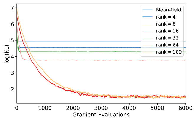
Figure 5: KL Convergence result for Gaussian inferential models with rank $p=4,8,16,32$ with $6000$ epochs. Inferential models with high ranks can achieve higher statistical accuracy in the case of sufficient computational budget on Gaussian Posterior.

E.2 Dataset Information

The original cardiac arrhythmia dataset (Dua and Graff,, 2017) aims to distinguish the presence of different types of cardiac arrhythmia in the patients, and classify each medical record into 16 subtypes using linear-valued and nominal features. We preprocess the data to project the original feature space into a subspace with dimension $d=110$, so as to effectively capture the covariance structure of the dataset. $Z$-score normalization is performed to standardize features for performance and convergence concerns. A binary target variable is then introduced based on the presence of different types of cardiac arrhythmia.

Many such features are not Gaussian distributed and are heavily correlated, posing difficulties for inference and causing mean-field variational approximation family to have large bias. As a result, more flexible inferential models are desirable to deal with the practical data. On the other hand, a noticeable amount of these features are independent to each other and contribute little to the classification result. Unlike the mean-field Gaussian family, the low-rank Gaussian inferential models excel at capturing the inherent dependence of data yet providing computational efficiency.

E.3 Experimental setup

We aim to provide a variational approximation $q_{(U,\Lambda)}(\theta|\mathbf{x})=\mathcal{N}(\mu,\Omega^{-1})$ to the posterior $p(\theta\,|\,\mathbf{x})$ of the cardiac arrhythmia dataset, where the precision matrix of the variational family is parameterized as $\Omega=\alpha\mathrm{I}_{d}+U\Lambda U^{\top}$. Rank $p$ is varied to study the statistical and computational trade-offs. We focus on learning the low-rank components of the precision matrix and set the diagonal structure to be isotropic with some positive constant $\alpha$ for simplicity. We then run the preconditioned SGD (algorithm 2) to sequentially optimize $U$ and $\Lambda$ with respect to the KL divergence until convergence is achieved. To compare with the mean-field family, we parameterize the precision matrix as $\Omega=\mathrm{diag}(u_{0}^{2})$ with diagonal structure only, and optimize $u_{0}$ using the same approach. In both inferential models, optimal fixed learning rates are applied.

Note that in contrast to the learning process of the mean vector $\mu$ in the inferential models, optimizing the precision matrix $\Omega$ tends to be much more computationally expensive in practice. To study the trade-offs, it is therefore sufficient to fix $\mu$ to be the estimated result returned by NUTS sampler, and optimize $\Omega$ only. The estimation result of $\mu$ is obtained from 20k samples generated from 2 parallel chains when using the NUTS algorithm. For initialization, we adopt a prior distribution $p(\theta)=\mathcal{N}(\mu,\beta\mathrm{I}_{d})$ with some positive number $\beta$ for both $U$ and $\Lambda$.

Results are averaged over 30 random seeds, with each optimized over $6000$ training epochs, reported along with the $95\%$ confidence interval respectively.

E.4 Additional plots of the Bayesian logistic regression study

We compare the Frobenius norm difference between baseline $\Omega^{*}$ obtained by the NUTS and the precision matrix $\Omega$ of the inferential models with rank $p=4,8,16,32$. The complete convergence result is provided in Figure 6. It suggests given sufficient computational budget, higher statistical accuracy can be achieved with the more flexible high-rank inferential models. Moreover, we have shown in Figure 4 that the low-rank Gaussian inferential models outperform the standard mean-field family. More specifically, Figure 8 compares bivariate marginals of the rank-$8$ inferential model and the mean-field one versus baseline obtained from the NUTS. We expect the performance difference to become more significant when the correlation among data is stronger.

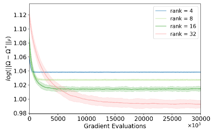
Figure 6: Convergence result for optimal low-rank inferential models with rank $p=4,8,16,32$ with $6000$ epochs. Inferential models with high ranks can achieve higher statistical accuracy in the case of sufficient computational budget on Cardiac arrhythmia dataset.

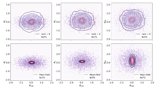
Figure 8: Low-rank inferential models lead to better approximation compared to mean-field family. Bivariate marginals of both inference models are compared against NUTS baseline for selected dimensions. Each distribution contour graph results from $3,000$ samples drawn from the baseline and its variational approximation. Top: bivariate marginals of low-rank inference model with rank $p=8$ against NUTS baseline. Bottom: bivariate marginals of mean-field model against NUTS baseline.

Appendix F Future Works

Extending the results in this paper to understand the statistical and computational trade-offs in other classes of inferential models is a promising avenue of future work. In particular, consider the mixture models. Another venue of possible extension is to provably improve the convergence of the variational inference methods, e.g. leveraging gradient descent over the Bures–Wasserstein manifold for fast convergence towards the stationary solution (Lambert et al.,, 2022).

References

• Alquier and Ridgway, (2017) Alquier, P. and Ridgway, J. (2017). Concentration of tempered posteriors and of their variational approximations. arXiv preprint arXiv:1706.09293.
• Alquier et al., (2016) Alquier, P., Ridgway, J., and Chopin, N. (2016). On the properties of variational approximations of gibbs posteriors. Journal of Machine Learning Research, 17(239):1–41.
• Araki, (1990) Araki, H. (1990). On an inequality of Lieb and Thirring. Letters in Mathematical Physics, 19(2):167–170.
• Balakrishnan et al., (2011) Balakrishnan, S., Kolar, M., Rinaldo, A., Singh, A., and Wasserman, L. (2011). Statistical and computational tradeoffs in biclustering. NIPS 2011 Workshop on Computational Trade-offs in Statistical Learning, 4.
• Balcan et al., (2016) Balcan, M.-F., Du, S. S., Wang, Y., and Yu, A. W. (2016). An improved gap-dependency analysis of the noisy power method. 29th Annual Conference on Learning Theory (COLT), 49:284–309.
• Banerjee et al., (2021) Banerjee, I., Rao, V. A., and Honnappa, H. (2021). PAC-Bayes bounds on variational tempered posteriors for markov models. arXiv preprint arXiv:2101.05197.
• Berthet et al., (2014) Berthet, Q. et al. (2014). Statistical and computational tradeoffs in high-dimensional problems.
• Bhattacharya et al., (2020) Bhattacharya, S., Liu, Z., and Maiti, T. (2020). Variational Bayes neural network: Posterior consistency, classification accuracy and computational challenges. arXiv preprint arXiv:2011.09592.
• Bhattacharya and Maiti, (2021) Bhattacharya, S. and Maiti, T. (2021). Statistical foundation of variational Bayes neural networks. Neural Networks, 137:151–173.
• Bickel et al., (2013) Bickel, P., Choi, D., Chang, X., Zhang, H., et al. (2013). Asymptotic normality of maximum likelihood and its variational approximation for stochastic blockmodels. The Annals of Statistics, 41(4):1922–1943.
• Blei et al., (2017) Blei, D. M., Kucukelbir, A., and McAuliffe, J. D. (2017). Variational inference: A review for statisticians. Journal of the American Statistical Association, 112(518):859–877.
• Calandriello and Rosasco, (2018) Calandriello, D. and Rosasco, L. (2018). Statistical and computational trade-offs in kernel k-means. Advances in Neural Information Processing Systems, 31:9357–9367.
• Campbell and Li, (2019) Campbell, T. and Li, X. (2019). Universal boosting variational inference. Advances in Neural Information Processing Systems, 32.
• Celisse et al., (2012) Celisse, A., Daudin, J.-J., Pierre, L., et al. (2012). Consistency of maximum-likelihood and variational estimators in the stochastic block model. Electronic Journal of Statistics, 6:1847–1899.
• Chandrasekaran and Jordan, (2013) Chandrasekaran, V. and Jordan, M. I. (2013). Computational and statistical tradeoffs via convex relaxation. Proceedings of the National Academy of Sciences, 110(13):E1181–E1190.
• Chandrasekaran et al., (2010) Chandrasekaran, V., Parrilo, P. A., and Willsky, A. S. (2010). Latent variable graphical model selection via convex optimization. pages 1610–1613.
• Chen and Ryzhov, (2020) Chen, Y. and Ryzhov, I. O. (2020). Consistency analysis of sequential learning under approximate Bayesian inference. Operations Research, 68(1):295–307.
• Chen et al., (2017) Chen, Y.-C., Wang, Y. S., and Erosheva, E. A. (2017). On the use of bootstrap with variational inference: Theory, interpretation, and a two-sample test example. arXiv preprint arXiv:1711.11057.
• Cheng et al., (2018) Cheng, X., Chatterji, N. S., Abbasi-Yadkori, Y., Bartlett, P. L., and Jordan, M. I. (2018). Sharp convergence rates for Langevin dynamics in the nonconvex setting. arXiv:1805.01648.
• Chérief-Abdellatif, (2019) Chérief-Abdellatif, B.-E. (2019). Consistency of ELBO maximization for model selection. Symposium on Advances in Approximate Bayesian Inference, pages 11–31.
• Chérief-Abdellatif, (2020) Chérief-Abdellatif, B.-E. (2020). Convergence rates of variational inference in sparse deep learning. pages 1831–1842.
• Chérief-Abdellatif et al., (2018) Chérief-Abdellatif, B.-E., Alquier, P., et al. (2018). Consistency of variational Bayes inference for estimation and model selection in mixtures. Electronic Journal of Statistics, 12(2):2995–3035.
• Dalalyan, (2017) Dalalyan, A. S. (2017). Theoretical guarantees for approximate sampling from smooth and log-concave densities. J. Royal Stat. Soc. B, 79(3):651–676.
• Dasarathy et al., (2017) Dasarathy, G., Rao, N., and Baraniuk, R. (2017). On computational and statistical tradeoffs in matrix completion with graph information.
• Dennis and Schnabel, (1983) Dennis, J. E., J. and Schnabel, R. B. (1983). Prentice-Hall.
• Dillon and Lebanon, (2009) Dillon, J. and Lebanon, G. (2009). Statistical and computational tradeoffs in stochastic composite likelihood. pages 129–136.
• Dua and Graff, (2017) Dua, D. and Graff, C. (2017). UCI machine learning repository.
• Freund et al., (2021) Freund, Y., Ma, Y.-A., and Zhang, T. (2021). When is the convergence time of Langevin algorithms dimension independent? A composite optimization viewpoint. arXiv preprint arXiv:2110.01827.
• Ghorbani et al., (2018) Ghorbani, B., Javadi, H., and Montanari, A. (2018). An instability in variational inference for topic models. arXiv preprint arXiv:1802.00568.
• Giordano et al., (2017) Giordano, R., Broderick, T., and Jordan, M. I. (2017). Covariances, robustness, and variational Bayes. arXiv preprint arXiv:1709.02536.
• Guha et al., (2020) Guha, B. S., Bhattacharya, A., and Pati, D. (2020). Statistical guarantees and algorithmic convergence issues of variational boosting. arXiv preprint arXiv:2010.09540.
• Hajargasht, (2019) Hajargasht, R. (2019). Approximation properties of variational Bayes for vector autoregressions. arXiv preprint arXiv:1903.00617.
• (33) Hall, P., Ormerod, J. T., and Wand, M. (2011a). Theory of Gaussian variational approximation for a Poisson mixed model. Statistica Sinica, pages 369–389.
• (34) Hall, P., Pham, T., Wand, M. P., Wang, S. S., et al. (2011b). Asymptotic normality and valid inference for Gaussian variational approximation. The Annals of Statistics, 39(5):2502–2532.
• Han and Yang, (2019) Han, W. and Yang, Y. (2019). Statistical inference in mean-field variational Bayes. arXiv preprint arXiv:1911.01525.
• Hardt and Price, (2014) Hardt, M. and Price, E. (2014). The noisy power method: A meta algorithm with applications. 27.
• Hoffman and Ma, (2020) Hoffman, M. and Ma, Y. (2020). Black-box variational inference as a parametric approximation to Langevin dynamics. 119:4324–4341.
• Hoffman et al., (2013) Hoffman, M. D., Blei, D. M., Wang, C., and Paisley, J. (2013). Stochastic variational inference. Journal of Machine Learning Research.
• Hoffman and Gelman, (2014) Hoffman, M. D. and Gelman, A. (2014). The No-U-Turn sampler. JMLR, 15(1):1593–1623.
• Hoffman and Ma, (2019) Hoffman, M. D. and Ma, Y. (2019). Langevin dynamics as nonparametric variational inference.
• Huggins et al., (2020) Huggins, J., Kasprzak, M., Campbell, T., and Broderick, T. (2020). Validated variational inference via practical posterior error bounds. pages 1792–1802.
• Huggins et al., (2018) Huggins, J. H., Campbell, T., Kasprzak, M., and Broderick, T. (2018). Practical bounds on the error of Bayesian posterior approximations: A nonasymptotic approach. arXiv preprint arXiv:1809.09505.
• Jaiswal et al., (2020) Jaiswal, P., Rao, V., and Honnappa, H. (2020). Asymptotic consistency of $\alpha$-rényi-approximate posteriors. Journal of Machine Learning Research, 21(156):1–42.
• Jin et al., (2020) Jin, Y., Wang, Z., and Lu, J. (2020). Computational and statistical tradeoffs in inferring combinatorial structures of Ising model. pages 4901–4910.
• Jordan et al., (1999) Jordan, M. I., Ghahramani, Z., Jaakkola, T. S., and Saul, L. K. (1999). An introduction to variational methods for graphical models. Machine learning, 37:183–233.
• Khetan and Oh, (2016) Khetan, A. and Oh, S. (2016). Computational and statistical tradeoffs in learning to rank. arXiv preprint arXiv:1608.06203.
• Khetan and Oh, (2018) Khetan, A. and Oh, S. (2018). Generalized rank-breaking: Computational and statistical tradeoffs. The Journal of Machine Learning Research, 19(1):983–1024.
• Knoblauch, (2019) Knoblauch, J. (2019). Frequentist consistency of generalized variational inference. arXiv preprint arXiv:1912.04946.
• Lambert et al., (2022) Lambert, M., Chewi, S., Bach, F., Bonnabel, S., and Rigollet, P. (2022). Variational inference via Wasserstein gradient flows. arXiv preprint arXiv:2205.15902.
• Li et al., (2016) Li, X., Xu, Y., Zhao, T., and Liu, H. (2016). Statistical and computational tradeoff of regularized dantzig-type estimators.
• Lu et al., (2018) Lu, H., Cao, Y., Yang, Z., Lu, J., Liu, H., and Wang, Z. (2018). The edge density barrier: Computational-statistical tradeoffs in combinatorial inference. pages 3247–3256.
• Ma et al., (2021) Ma, Y.-A., Chatterji, N. S., Cheng, X., Flammarion, N., Bartlett, P. L., and Jordan, M. I. (2021). Is there an analog of Nesterov acceleration for MCMC? Bernoulli, 27(3):1942–1992.
• Ma et al., (2019) Ma, Y.-A., Chen, Y., Jin, C., Flammarion, N., and Jordan, M. I. (2019). Sampling can be faster than optimization. Proc. Natl. Acad. Sci. U.S.A., 116(42):20881–20885.
• Medina et al., (2021) Medina, M. A., Olea, J. L. M., Rush, C., and Velez, A. (2021). On the robustness to misspecification of $alpha$-posteriors and their variational approximations. arXiv preprint arXiv:2104.08324.
• Miller et al., (2017) Miller, A. C., Foti, N. J., and Adams, R. P. (2017). Variational boosting: Iteratively refining posterior approximations. International Conference on Machine Learning, pages 2420–2429.
• Mukherjee and Sen, (2021) Mukherjee, S. and Sen, S. (2021). Variational inference in high-dimensional linear regression. arXiv preprint arXiv:2104.12232.
• Mukherjee and Sarkar, (2018) Mukherjee, S. S. and Sarkar, P. (2018). Mean field for the stochastic blockmodel: Optimization landscape and convergence issues. Advances in Neural Information Processing Systems.
• Nesterov, (2004) Nesterov, Y. (2004). Introductory Lectures on Convex Optimization: A Basic Course. Kluwer, Boston.
• O’Hara et al., (2009) O’Hara, R. B., Sillanpää, M. J., et al. (2009). A review of Bayesian variable selection methods: what, how and which. Bayesian analysis, 4(1):85–117.
• Otto and Villani, (2000) Otto, F. and Villani, C. (2000). Generalization of an inequality by talagrand and links with the logarithmic sobolev inequality. Journal of Functional Analysis, 173(2):361–400.
• Pati et al., (2017) Pati, D., Bhattacharya, A., and Yang, Y. (2017). On statistical optimality of variational Bayes. arXiv preprint arXiv:1712.08983.
• Plummer et al., (2020) Plummer, S., Pati, D., and Bhattacharya, A. (2020). Dynamics of coordinate ascent variational inference: A case study in 2d Ising models. Entropy, 22(11):1263.
• Ramdas et al., (2015) Ramdas, A., Reddi, S. J., Poczos, B., Singh, A., and Wasserman, L. (2015). Adaptivity and computation-statistics tradeoffs for kernel and distance based high dimensional two sample testing. arXiv preprint arXiv:1508.00655.
• Ray and Szabó, (2021) Ray, K. and Szabó, B. (2021). Variational Bayes for high-dimensional linear regression with sparse priors. Journal of the American Statistical Association, pages 1–12.
• Ray et al., (2020) Ray, K., Szabo, B., and Clara, G. (2020). Spike and slab variational Bayes for high dimensional logistic regression. arXiv preprint arXiv:2010.11665.
• Sarkar et al., (2021) Sarkar, P., Wang, Y. R., and Mukherjee, S. S. (2021). When random initializations help: A study of variational inference for community detection. Journal of Machine Learning Research, 22(22):1–46.
• Sheth and Khardon, (2017) Sheth, R. and Khardon, R. (2017). Excess risk bounds for the Bayes risk using variational inference in latent Gaussian models. Advances in Neural Information Processing Systems, pages 5157–5167.
• Song et al., (2020) Song, Q., Sun, Y., Ye, M., and Liang, F. (2020). Extended stochastic gradient mcmc for large-scale Bayesian variable selection. arXiv preprint arXiv:2002.02919.
• Sriperumbudur and Sterge, (2017) Sriperumbudur, B. and Sterge, N. (2017). Approximate kernel PCA using random features: Computational vs. statistical trade-off. arXiv preprint arXiv:1706.06296.
• Wainwright and Jordan, (2008) Wainwright, M. J. and Jordan, M. I. (2008). Graphical models, exponential families, and variational inference. Foundations and Trends® in Machine Learning, 1(1-2):1–305.
• Wang and Titterington, (2004) Wang, B. and Titterington, D. (2004). Convergence and asymptotic normality of variational Bayesian approximations for exponential family models with missing values. Proceedings of the 20th conference on Uncertainty in Artificial Intelligence, pages 577–584.
• Wang et al., (2006) Wang, B., Titterington, D., et al. (2006). Convergence properties of a general algorithm for calculating variational Bayesian estimates for a normal mixture model. Bayesian Analysis, 1(3):625–650.
• Wang et al., (2019) Wang, L., Yang, Z., and Wang, Z. (2019). Statistical-computational tradeoff in single index models. Advances in Neural Information Processing Systems, 32:10419–10426.
• Wang et al., (2016) Wang, T., Berthet, Q., Samworth, R. J., et al. (2016). Statistical and computational trade-offs in estimation of sparse principal components. The Annals of Statistics, 44(5):1896–1930.
• Wang and Blei, (2019) Wang, Y. and Blei, D. (2019). Variational Bayes under model misspecification. Advances in Neural Information Processing Systems, 32.
• Wang and Blei, (2018) Wang, Y. and Blei, D. M. (2018). Frequentist consistency of variational Bayes. Journal of the American Statistical Association, (just-accepted):1–85.
• Welandawe et al., (2022) Welandawe, M., Andersen, M. R., Vehtari, A., and Huggins, J. H. (2022). Robust, automated, and accurate black-box variational inference. arXiv preprint arXiv:2203.15945.
• Westling and McCormick, (2015) Westling, T. and McCormick, T. H. (2015). Establishing consistency and improving uncertainty estimates of variational inference through M-estimation. arXiv preprint arXiv:1510.08151.
• Womack et al., (2013) Womack, A. J., Moreno, E., and Casella, G. (2013). Consistency in latent allocation models.
• Xu and Campbell, (2021) Xu, Z. and Campbell, T. (2021). The computational asymptotics of Gaussian variational inference. arXiv preprint arXiv:2104.05886.
• Yang and Martin, (2020) Yang, Y. and Martin, R. (2020). Variational approximations of empirical Bayes posteriors in high-dimensional linear models. arXiv preprint arXiv:2007.15930.
• Yang et al., (2017) Yang, Y., Pati, D., and Bhattacharya, A. (2017). $\alpha$-variational inference with statistical guarantees. arXiv preprint arXiv:1710.03266.
• Yang et al., (2016) Yang, Y., Wainwright, M. J., Jordan, M. I., et al. (2016). On the computational complexity of high-dimensional Bayesian variable selection. Annals of Statistics, 44(6):2497–2532.
• Yi et al., (2019) Yi, X., Wang, Z., Yang, Z., Caramanis, C., and Liu, H. (2019). More supervision, less computation: statistical-computational tradeoffs in weakly supervised learning. arXiv preprint arXiv:1907.06257.
• You et al., (2014) You, C., Ormerod, J. T., and Müller, S. (2014). On variational Bayes estimation and variational information criteria for linear regression models. Australian & New Zealand Journal of Statistics, 56(1):73–87.
• Zhang and Zhou, (2017) Zhang, A. Y. and Zhou, H. H. (2017). Theoretical and computational guarantees of mean field variational inference for community detection. arXiv preprint arXiv:1710.11268.
• Zhang and Gao, (2017) Zhang, F. and Gao, C. (2017). Convergence rates of variational posterior distributions. arXiv preprint arXiv:1712.02519.