A Hybrid Numerical Algorithm for Evaluating n-th Order Tridiagonal Determinants

Abstract

The principal minors of a tridiagonal matrix satisfy two-term and three-term recurrences [1, 2]. Based on these facts, the current article presents a new efficient and reliable hybrid numerical algorithm for evaluating general n-th order tridiagonal determinants in linear time. The hybrid numerical algorithm avoid all symbolic computations. The algorithm is suited for implementation using computer languages such as FORTRAN, PASCAL, ALGOL, MAPLE, MACSYMA and MATHEMATICA. Some illustrative examples are given. Test results indicate the superiority of the hybrid numerical algorithm.

1 Introduction

A general tridiagonal matrix $T_{n}=(t_{ij})_{1\leq i,j\leq n}$ takes the form:

$$T_{n}=(t_{ij})=\left[\begin{array}[]{cccccc}d_{1}&a_{1}&0&\cdots&\cdots&0\\ b_{1}&d_{2}&a_{2}&\ddots&&\vdots\\ 0&b_{2}&d_{3}&\ddots&0&\vdots\\ \vdots&\ddots&\ddots&\ddots&\ddots&0\\ \vdots&&0&\ddots&\ddots&a_{n-1}\\ 0&\cdots&\cdots&0&b_{n-1}&d_{n}\\ \end{array}\right]_{n},n\geq 3$$ (1)

in which $t_{ij}=0$ whenever $|i-j|>1$.
These matrices arise frequently in a wide range of scientific and engineering fields [3, 4, 5, 6]. For instance, telecommunication, parallel computing, and statistics. For the matrix $T_{n}$ in (1), there is no need to store the zero elements. Consequently, we can use three vectors $\mathbf{a}=(a_{1},a_{2},\cdots,a_{n-1})$, $\mathbf{b}=(b_{1},b_{2},\cdots,b_{n-1})$, and $\mathbf{d}=(d_{1},d_{2},\cdots,d_{n})$ to store the non-zero elements of $T_{n}$ in $3n-2$ memory locations rather than $n^{2}$ for a full matrix. This is always a good habit in computation. When we consider the matrix $T_{n}$ in (1), it is useful to add an additional n-dimensional vector $\mathbf{c}=(c_{1},c_{2},\cdots,c_{n})$ given by:

$$c_{i}=\left\{\begin{array}[]{lr}d_{1}&\text{if}\quad i=1,\\ d_{i}-a_{i-1}b_{i-1}/c_{i-1}&\text{if}\quad i=2,3,\cdots,n\end{array}\right.$$ (2)

By adding this vector $\mathbf{c}$ , we are able to:
(i) evaluate $det(T_{n})$ in linear time [1],
(ii) write down the Doolittle and Crout LU factorizations of the matrix $T_{n}$ [7], and
(iii) check whether or not a symmetric tridiagonal matrix $T_{n}$ is the positive definite. In fact if $T_{n}$ is symmetric then it is positive definite if and only if $c_{i}>0,i=1,2,\cdots,n$ [7].

In [8], the following question has been raised:
Is there a fast way to prove that the tridiagonal matrix

$$A=\left[\begin{array}[]{ccccc}4&2&0&0&0\\ 2&5&2&0&0\\ 0&2&5&2&0\\ 0&0&2&5&2\\ 0&0&0&2&5\\ \end{array}\right]$$

is a positive definite?
Our answer is: $A$ is actually positive definite since $c_{i}=4>0,i=1,2,3,4,5$ as can be easily checked. This is the easiest way to check the positive definiteness of a symmetric tridiagonal matrix.

The current article is organized as follows. The main result is presented in Section 2. In Section 3, numerical tests and some illustrative examples are given. The conclusion is presented in Section 4.

2 The Main Result

This section is mainly devoted to constructs a hybrid numerical algorithm for evaluating n-th order tridiagonal determinant of the form (1).
Let:

$$f_{1}=|d_{1}|=d_{1},f_{i}=\left|\begin{array}[]{cccccc}d_{1}&a_{1}&0&\cdots&\cdots&0\\ b_{1}&d_{2}&a_{2}&\ddots&&\vdots\\ 0&b_{2}&d_{3}&\ddots&0&\vdots\\ \vdots&\ddots&\ddots&\ddots&\ddots&0\\ \vdots&&0&\ddots&\ddots&a_{i-1}\\ 0&\cdots&\cdots&0&b_{i-1}&d_{i}\\ \end{array}\right|,i=2,3,\cdots.n$$ (3)

Therefore, $f_{i},i=1,2,\cdots,n$ are the principal minors of $T_{n}$. The determinants in (3) satisfy a two-term recurrence [2]

$$f_{i}=\prod_{r=1}^{i}c_{r}=c_{i}f_{i-1},i=1,2,\cdots,n,f_{0}=1$$ (4)

The three-term recurrence

$$f_{i}=d_{i}f_{i-1}-a_{i-1}b_{i-1}f_{i-2},i=2,3,\cdots,n,f_{0}=1,f_{1}=d_{1}$$ (5)

is also valid [2].
For convenience of the reader it is convenient to describe the DETGTRI algorithm in which $z$ is just a symbolic name [1].

Algorithm 1 DETGTRI

Input: $n$ and the components of the vectors $\mathbf{a},\mathbf{b}$, and $\mathbf{d}$.
Output: $det(T_{n})$.
Step 1: For $k$ from $2$ to $n$ do
                  Compute and simplify:
                  If $d_{k-1}=0$ then $d_{k-1}=z$ end if.
                  $d_{k}:=d_{k}-a_{k-1}b_{k-1}/d_{k-1}$
             End do
Step 2: Compute $P(z)=\prod_{r=1}^{n}d_{r}$
Step 3: Set $det(T_{n})=P(0)$.

Based on the three-term recurrence (5), we may formulate the following algorithm.

Algorithm 2

Input: $n$ and the components of the vectors $\mathbf{a},\mathbf{b}$, and $\mathbf{d}$.
Output: $det(T_{n})$.
Step 1: Set $f_{0}=1$ and $f_{1}=d_{1}$.
Step 2: For $i$ from $2$ to $n$ do
                  $f_{i}=d_{i}f_{i-1}-a_{i-1}b_{i-1}f_{i-2}$,
             End do.
Step 3: Set $det(T_{n})=f_{n}$.

At this stage, we present the following hybrid numerical algorithm.

Algorithm 3

Input: $n$ and the components of the vectors $\mathbf{a},\mathbf{b}$, and $\mathbf{d}$.
Output: $det(T_{n})$.
Step 1: Set $c_{1}=d_{1}$, $f_{1}=d_{1}$, and $m=1$.
Step 2: While $m\leq n-1$ and $c_{m}\neq 0$ do
                  $m=m+1$,
                  $c_{m}=d_{m}-a_{m-1}b_{m-1}/c_{m-1}$,
                 $f_{m}=c_{m}f_{m-1}$,
             End do.
Step 3: For $k=m+1$ to $n$ do
                  $f_{k}=d_{k}f_{k-1}-a_{k-1}b_{k-1}f_{k-2}$
             End do.
Step 4: Set $det(T_{n})=f_{n}$.

The hybrid numerical algorithm has the same computational cost as the algorithms DETGTRI and Algorithm 2. Algorithm 3 links two methods and has the advantage that no symbolic computations are involved.
Remark: It should be noted that Step 3 in Algorithm 3 is redundant and will not be executed at all if $c_{i}\neq 0,i=1,2,\cdots,n-1$. Therefore, we only need Step 1, Step 2 and Step 4. For positive definite and strictly diagonally dominant matrices, this is always the case. The implementation of the hybrid numerical algorithm using any computer language are straight forward.

3 Numerical Tests and Illustrative Examples

In this section, we are going to consider Some numerical tests and illustrative examples. All computations are carried out using laptop machine with a 2.50GHz CPU, 8GB of RAM, AMD A10-9620P RADEON R5 processor and Maple 2021.
Example 3.1. Consider the tridiagonal matrix $T_{n}$, with $n=4$ given by:

                           $T_{n}=(t_{ij})=\left[\begin{array}[]{cccc}1&1&0&0\\ 1&1&-1&0\\ 0&1&2&1\\ 0&0&-3&-1\\ \end{array}\right]_{4}$
Find $det(T_{n})$.
Solution:
We have:
$a_{1}=1,a_{2}=-1,a_{3}=1,b_{1}=1,b_{2}=1,b_{3}=-3,d_{1}=1,d_{2}=1,d_{3}=2,$ and $d_{4}=-1$.
By applying the Algorithm 3, we obtain
Step 1: $c_{1}=d_{1}=1$, $f_{1}=d_{1}=1$ and $m=1$
Step 2: $m=2,c_{2}=0,f_{2}=c_{2}f_{1}=0$.
Step 3: $f_{3}=d_{3}f_{2}-a_{2}b_{2}f_{1}=(2)(0)-(-1)(1)(1)=1,$ and $f_{4}=d_{4}f_{3}-a_{3}b_{3}f_{2}=(-1)(1)-(1)(-3)(0)=-1$.
Step 4: $det(T_{n})=f_{4}=-1$.

Example 3.2. Consider $T_{n},$ with $n=9$, given by:
$a_{i}=-1,b_{i}=-1,d_{i}=2,i=1,2,\cdots,n-1,$ and $d_{n}=2$.
By applying the Algorithm 3, we get
Step 1: $c_{1}=2$, and $f_{1}=2$.
Step 2:

$$m$$ 2 3 4 5 6 7 8 9

3 4 5 6 7 8 9 10

Step 4: $det(T_{n})=f_{9}=10$.

Example 3.3. Let $T_{n}$ is given by:
                           $T_{n}=(t_{ij})\left[\begin{array}[]{cccccc}1&1&0&\cdots&\cdots&0\\ 1&1&1&\ddots&&\vdots\\ 0&1&1&\ddots&0&\vdots\\ \vdots&\ddots&\ddots&\ddots&\ddots&0\\ \vdots&&0&1&1&1\\ 0&\cdots&\cdots&0&1&1\\ \end{array}\right]_{n}$
By using (4), we get:
$det(T_{n})=\left\{\begin{array}[]{lr}1&\text{if}\quad n\equiv 0\quad or\quad 1\quad mod(6),\\ 0&\text{if}\quad n\equiv 2\quad or\quad 5\quad mod(6),\\ -1&\text{if}\quad n\equiv 3\quad or\quad 4\quad mod(6).\end{array}\right.$

Now, it is time to consider Example 3.3 as a test problem to compare the three algorithms and the MATLAB function $det()$. For these algorithms, we get the results presented in Table 1. The DETGTRI algorithm involves symbolic computations since $c_{2}=0$.

Table 1: The CPU times of DETGTRI, Algorithm 2, Algorithm 3 and MATLAB function($det()$) for Example 3.3

$n$	DETGTRI	Algorithm 2	Algorithm 3	MATLAB ($det()$)
	CPU time(s)	CPU time(s)	CPU time(s)	CPU time(s)
10000	0.782	0.329	0.078	55.191
20000	1.516	0.672	0.172	342.727
30000	2.188	1.063	0.485	1636.835
40000	3.109	1.297	0.500	–
50000	3.906	1.937	0.640	–
100000	7.437	4.218	0.796	–

Table 1 shows that the Algorithm 3 is superior comparing with the DETGTRI algorithm. The MATLAB function $det()$ has the largest CPU time between all algorithms.

Example 3.4. Consider the matrix $T_{n}$ given by:
                           $T_{n}=(t_{ij})\left[\begin{array}[]{ccccccc}1&1&0&\cdots&\cdots&\cdots&0\\ n-1&1&2&\ddots&&&\vdots\\ 0&n-2&1&3&\ddots&&\vdots\\ \vdots&&\ddots&\ddots&\ddots&&0\\ \vdots&&&&2&1&n-1\\ 0&\cdots&\cdots&\cdots&0&1&1\\ \end{array}\right]_{n}$

Consider $det(T_{n})$. The DETGTRI algorithm gives:

$$c_{k}=\left\{\begin{array}[]{lr}\qquad k&\text{if}\quad k\quad\text{is odd}\\ -(n-k)&\text{if}\quad k\quad\text{is even}\end{array}\right.$$

Therefore,

$$det(T_{n})=\prod_{r=1}^{n}c_{r}=\left\{\begin{array}[]{lr}\qquad 0&\text{if}\quad n\quad\text{is even}\\ \frac{(-1)^{\frac{n-1}{2}}n!}{2^{n-1}}\binom{n-1}{\frac{n-1}{2}}&\text{if}\quad n\quad\text{is odd}\end{array}\right.$$

on simplification. Note that $det(T_{n})=0$ when $n$ is even although $c_{i}\neq 0$ for $i=1,2,\cdots,n-1$. This is because $c_{n}=0$.
In Table 2, we list some numerical results for DETGTRI algorithm, Algorithm 2 and Algorithm 3. The superiority of Algorithm 3 is obvious in Fig. 1.

Table 2: Comparing DETGTRI algorithm, Algorithm 2 and Algorithm 3 for Example 3.4

$n$	DETGTRI	Algorithm 2	Algorithm 3
	CPU time(s)	CPU time(s)	CPU time(s)
1000	0.109	0.063	0.047
1500	0.140	0.094	0.062
2000	0.156	0.105	0.078
2500	0.172	0.125	0.092
3000	0.250	0.152	0.128

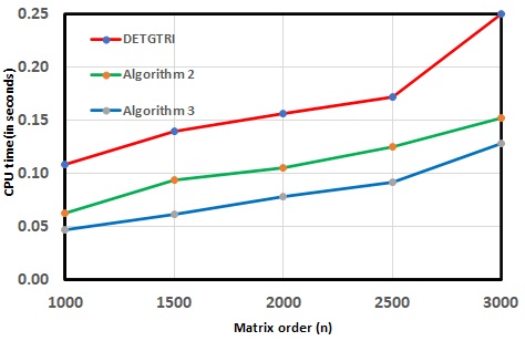
Figure 1: Efficiency of the DETGTRI algorithm, Algorithm 2 and Algorithm 3

Example 3.5. Consider the matrix $T_{n}$ given by:
                           $T_{n}=(t_{ij})\left[\begin{array}[]{ccccccc}1&1&0&\cdots&\cdots&\cdots&0\\ 2&2&1&\ddots&&&\vdots\\ 0&2&2&1&\ddots&&\vdots\\ \vdots&&\ddots&\ddots&\ddots&&0\\ \vdots&&&&2&2&1\\ 0&\cdots&\cdots&\cdots&0&2&1\\ \end{array}\right]_{n}$

In this example, $c_{2}=0$. So, the DETGTRI algorithm contains symbolic computations. Table 3 shows the CPU times for the three algorithms. The Algorithm 3 has CPU time less than the other two algorithms.

Table 3: Comparing DETGTRI algorithm, Algorithm 2 and Algorithm 3 for Example 3.5

$n$	DETGTRI	Algorithm 2	Algorithm 3
	CPU time(s)	CPU time(s)	CPU time(s)
1000	1.3440	0.0437	0.0031
1500	1.6250	0.0547	0.0125
2000	1.8600	0.0626	0.0140
2500	2.4690	0.0688	0.0186
3000	2.7650	0.0985	0.0265

Fig. 2 displays the logarithm of the CPU times multiplied by 1000 versus the matrix order $n$. Based on this figure, the Algorithm 2 has least CPU times between all three algorithms.

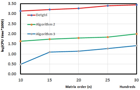
Figure 2: Efficiency of the DETGTRI algorithm, Algorithm 2 and Algorithm 3

4 Conclusion

In this paper, a hybrid numerical algorithm (Algorithm 3) has been derived for evaluating general n-th order tridiagonal determinants in linear time. The algorithm avoids all symbolic computations. The results show how effective the hybrid numerical algorithm is.

References

- [1] M. E. A. El-Mikkawy, A fast algorithm for evaluating nth order tri-diagonal determinants, Journal of Computational and Applied Mathematics 166 (2) (2004) 581–584. doi:https://doi.org/10.1016/j.cam.2003.08.044.
- [2] M. E. A. El-Mikkawy, A note on a three-term recurrence for a tridiagonal matrix, Applied Mathematics and Computation 139 (2) (2003) 503–511. doi:https://doi.org/10.1016/S0096-3003(02)00212-6.
-
[3]
L. G. Molinari,
Determinants
of block tridiagonal matrices, Linear Algebra and its Applications 429 (8)
(2008) 2221–2226.
doi:https://doi.org/10.1016/j.laa.2008.06.015.
URL https://www.sciencedirect.com/science/article/pii/S0024379508003200 - [4] J. Jina, P. Trojovsky, On determinants of some tridiagonal matrices connected with fibonacci numbers, International Journal of Pure and Applied Mathematics 88. doi:10.12732/ijpam.v97i1.8.
-
[5]
J. Jia, S. Li,
On
the inverse and determinant of general bordered tridiagonal matrices,
Computers Mathematics with Applications 69 (6) (2015) 503–509.
doi:https://doi.org/10.1016/j.camwa.2015.01.012.
URL https://www.sciencedirect.com/science/article/pii/S089812211500036X - [6] F. Qi, W. Wang, B.-N. Guo, D. Lim, Several explicit and recurrent formulas for determinants of tridiagonal matrices via generalized continued fractions, in: Z. Hammouch, H. Dutta, S. Melliani, M. Ruzhansky (Eds.), Nonlinear Analysis: Problems, Applications and Computational Methods, Springer International Publishing, Cham, 2021, pp. 233–248.
- [7] J. F. R.L. Burden, Numerical Analysis, 7th Edition, Brooks Cole Publishing, Pacific Grove, CA, 2001.
- [8] https://math.stackexchange.com/questions/2776864/is-there-a-fast-way-to-prove-a-tridiagonal-matrix-is-positive-definite.