Dirac-boson stars

Abstract

In this paper, we construct Dirac-boson stars (DBSs) model composed of a scalar field and two Dirac fields. The scalar field and both Dirac fields are in the ground state. We consider the solution families of the DBSs for the synchronized frequency $\tilde{\omega}$ and the nonsynchronized frequency $\tilde{\omega}_{D}$ cases, respectively. We find several different solutions when the Dirac mass $\tilde{\mu}_{D}$ and scalar field frequency $\tilde{\omega}_{S}$ are taken in some particular ranges. In contrast, no similar case has been found in previous studies of multistate boson stars. Moreover, we discuss the characteristics of each type of solution family of the DBSs and present the relationship between the ADM mass $M$ of the DBSs and the synchronized frequency $\tilde{\omega}$ or the nonsynchronized frequency $\tilde{\omega}_{D}$. Finally, we calculate the binding energy $E_{B}$ of the DBSs and investigate the relationship of $E_{B}$ with the synchronized frequency $\tilde{\omega}$ or the nonsynchronized frequency $\tilde{\omega}_{D}$.

I Introduction

In the 1950s, J. A. Wheeler studied the classical fields of electromagnetism coupled to Einstein’s gravity, and obtained an unstable solution, so-called geons Wheeler:1955zz ; Power:1957zz . In 1968, D. J. Kaup constructed the theory of complex scalar field coupled to Einstein gravity Kaup:1968zz , called the Einstein-Klein-Gordon theory. He found a stable solution of this configuration. Related work was subsequently done by R. Ruffini and S. Bonazzola Ruffini:1969qy . Solitons formed by scalar fields under their gravity are called Boson stars (BSs). In astrophysics, BSs are thought to be a possible component of dark matter Sahni:1999qe ; Matos:2000ng ; Hu:2000ke ; Suarez:2013iw ; Hui:2016ltb ; Padilla:2019fju . Furthermore, BSs have been used to mimic the black holes Cardoso:2019rvt ; Herdeiro:2021lwl . More recently, BSs have been used to analyze gravitational-wave signal Bustillo:2020syj ; Bezares:2022obu .

BSs with a single complex scalar field of matter has been extensively studied. The BSs with self-interaction have been studied in Refs. Colpi:1986ye ; Mielke:1980sa ; Kling:2017hjm ; Herdeiro:2020jzx . In addition, coupling the complex scalar field with the electromagnetic field can be considered to obtain the charged boson stars Jetzer:1989av ; Jetzer:1992tog ; Kleihaus:2009kr ; Kumar:2014kna . Solving Einstein’s Klein-Gordon equation in the Newtonian limit yields the Newtonian boson stars harrison2002numerical . In addition, rotating bosons with angular momentum are studied in Refs. Schunck:1996he ; Yoshida:1997qf ; Kleihaus:2005me ; Hartmann:2010pm ; Kling:2020xjj . Einstein’s gravity can also be coupled to fields with non-zero spin. In 2015, Brito et al. Brito:2015pxa proposed the Einstein-Proca theory. They studied the static solutions of the system in which the Proca field (spin-1) coupled to Einstein gravity, called Proca stars. Shortly afterward, I. Salazar Landea and F. García proposed the charged Proca stars SalazarLandea:2016bys . In addition, Finster et al. Finster:1998ws constructed a spherically symmetric system with two spinor fields (spin-1/2) and Einstein gravity coupling, which is the first study of the Dirac stars. Moreover, the coupling of the spinor field with the electromagnetic field can constitute the charged Dirac stars Finster:1998ux ; Bohun:1999zdr . In Ref. Dzhunushaliev:2018jhj , V. Dzhunushaliev and V. Folomeev studied the Dirac stars with self-interaction. More recently, the rotating Dirac stars were first proposed by Brito et al. Herdeiro:2019mbz . There are also other studies on the coupling of the spinor field with gravity Daka:2019iix ; Blazquez-Salcedo:2019qrz ; Blazquez-Salcedo:2019uqq ; Minamitsuji:2020hpl ; Leith:2021urf .

Also interesting are systems in which Einstein’s gravity is coupled to multiple matter fields. In Ref. Bernal:2009zy , Bernal et al. constructed a system consisting of two complex scalar fields in the ground state and the first excited state, respectively, called Multi-state Boson Stars (MSBS). Later, the rotating multistate boson stars were studied in Refs. Li:2019mlk ; Li:2020ffy . The matter fields of the spherically symmetric boson stars can be extended to an odd number $N$ of complex scalar fields Alcubierre:2018ahf ; Alcubierre:2019qnh . Systems in which the axion field and the complex scalar field are coupled are considered in Refs. Guerra:2019srj ; Delgado:2020udb and are called axion boson stars (ABSs). Multi-field models that include the Proca field have also been studied in Ref. Delgado:2020hwr . This work aims to solve Einstein-Dirac-Klein-Gordon equations numerically, construct the spherical Dirac-boson stars (DBSs) consisting of two spinor fields and a complex scalar field, and investigate the characteristics of various families of the solutions.

The paper is organized as follows. In Sec. II, we present the model four-dimensional Einstein gravity coupled to a complex massive scalar and two Dirac fields. In Sec. III, the boundary conditions of the Dirac boson stars are studied. We show the numerical results of the equations of motion and exhibit the properties of the multistate for two different cases in Sec. IV. We conclude in Sec. V with a summary and illustrate the range for future work.

II The model setup

we consider the system of two massive Dirac fields and a massive complex scalar field, which is minimally coupled to ($3+1$)-dimensional Einstein gravity. The action is given by

$$S=\int\sqrt{-g}d^{4}x\left(\frac{R}{16\pi G}+{\cal L}_{S}+{\cal L}_{D}\right)\,,$$ (1)

where $G$ is the gravitational constant, $R$ is the Ricci scalar, and ${\cal L}_{S}$ and ${\cal L}_{D}$ denote the Lagrangians of scalar and Dirac fields, respectively,

$${\cal L}_{S}=-g^{\alpha\beta}\partial_{\alpha}\psi^{*}\partial_{\beta}\psi-\mu_{S}^{2}\psi^{*}\psi\,,$$ (2)

$${\cal L}_{D}=-i\sum\limits_{k=1}^{2}\left[\frac{1}{2}\left(\hat{D}_{\mu}\overline{\Psi}^{(k)}\gamma^{\mu}\Psi^{(k)}-\overline{\Psi}^{(k)}\gamma^{\mu}\hat{D}_{\mu}\Psi^{(k)}\right)+\mu_{D}\overline{\Psi}^{(k)}\Psi^{(k)}\right]\,,$$ (3)

where $\mu_{S}$ and $\mu_{D}$ are the scalar field mass and the common mass of the Dirac fields, respectively. Here $\psi$ is a complex scalar field, $\Psi^{(k)}~{}(k=1,2)$ are the Dirac fields (to construct a spherically symmetric configuration, we need at least two spinors). $\overline{\Psi}^{(k)}=\Psi^{(k)\dagger}\zeta$ are the Dirac conjugate, with $\Psi^{(k)\dagger}$ stands for the Hermitian conjugate. For the Hermitizing matrix $\zeta$, we choose $\zeta=\gamma^{0}$ Dolan:2015eua . $\gamma^{\mu}$ are the gamma matrices in curved spacetime, $\hat{D}_{\mu}=\partial_{\mu}+\Gamma_{\mu}$ is the spinor covariant derivative, where $\Gamma_{\mu}$ are the spinor connection matrices. We show the details of the Dirac fields in the appendix. The field equations are given by

$$R_{\alpha\beta}-\frac{1}{2}g_{\alpha\beta}R=8\pi G\left(T^{S}_{\alpha\beta}+T^{D}_{\alpha\beta}\right)\,,$$ (4)

$$\nabla^{2}\psi-\mu_{S}^{2}\psi=0\,,$$ (5)

$$\gamma^{\mu}\hat{D}_{\mu}\Psi^{(k)}-\mu_{D}\Psi^{(k)}=0\,,$$ (6)

where $T^{S}_{\alpha\beta}$ and $T^{D}_{\alpha\beta}$ are the energy-momentum tensors of the scalar and Dirac fields, respectively,

$$T^{S}_{\alpha\beta}=\partial_{\alpha}\psi^{*}\partial_{\beta}\psi+\partial_{\beta}\psi^{*}\partial_{\alpha}\psi-g_{\alpha\beta}\left[\frac{1}{2}g^{\mu\nu}\left(\partial_{\mu}\psi^{*}\partial_{\nu}\psi+\partial_{\nu}\psi^{*}\partial_{\mu}\psi\right)+\mu_{S}^{2}\psi^{*}\psi\right]\,,$$ (7)

$$T^{D}_{\alpha\beta}=\sum\limits_{k=1}^{2}-\frac{i}{2}\left(\overline{\Psi}^{(k)}\gamma_{\alpha}\hat{D}_{\beta}\Psi^{(k)}+\overline{\Psi}^{(k)}\gamma_{\beta}\hat{D}_{\alpha}\Psi^{(k)}-\hat{D}_{\alpha}\overline{\Psi}^{(k)}\gamma_{\beta}\Psi^{(k)}-\hat{D}_{\beta}\overline{\Psi}^{(k)}\gamma_{\alpha}\Psi^{(k)}\right)\,.$$ (8)

The action of the matter fields are invariant under the $U(1)$ transformation $\psi\rightarrow e^{i\alpha}\psi$, $\Psi^{(k)}\rightarrow e^{i\alpha}\Psi^{(k)}$ with a constant $\alpha$. According to Noether’s theorem, there are conserved currents corresponding to these two matter fields:

$$J_{S}^{\mu}=-i\left(\psi^{*}\partial^{\mu}\psi-\psi\partial^{\mu}\psi^{*}\right),\qquad J_{D}^{\mu}=\overline{\Psi}\gamma^{\mu}\Psi\,.$$ (9)

Integrating the timelike component of these conserved currents on a spacelike hypersurface $\cal{S}$, then we can obtain the Noether charges:

$$Q_{S}=\int_{\cal S}J_{S}^{t}\,,\qquad Q_{D}=\int_{\cal S}J_{D}^{t}\,.$$ (10)

We will construct static spherically symmetric Dirac-boson stars, for which we should choose the following form of the spacetime metric:

$$ds^{2}=-N(r)\sigma^{2}(r)dt^{2}+\frac{dr^{2}}{N(r)}+r^{2}\left(d\theta^{2}+\sin^{2}\theta d\varphi^{2}\right)\,,$$ (11)

where $N(r)=1-{2m(r)}/{r}$, and the mass function $m(r)$ and $\sigma(r)$ depend only on the radial distance $r$. In addition, for the static spherically symmetric system, we use the following ansatz of the scalar and Dirac fields Herdeiro:2017fhv :

$$\psi=\phi(r)e^{-i\omega_{S}t}\,,$$ (12)

$$\Psi^{(1)}=\begin{pmatrix}\cos(\frac{\theta}{2})[(1+i)f(r)-(1-i)g(r)]\\ i\sin(\frac{\theta}{2})[(1-i)f(r)-(1+i)g(r)]\\ -i\cos(\frac{\theta}{2})[(1-i)f(r)-(1+i)g(r)]\\ -\sin(\frac{\theta}{2})[(1+i)f(r)-(1-i)g(r)]\end{pmatrix}e^{i\frac{\varphi}{2}-i\omega_{D}t}\,,$$ (13)

$$\Psi^{(2)}=\begin{pmatrix}i\sin(\frac{\theta}{2})[(1+i)f(r)-(1-i)g(r)]\\ \cos(\frac{\theta}{2})[(1-i)f(r)-(1+i)g(r)]\\ \sin(\frac{\theta}{2})[(1-i)f(r)-(1+i)g(r)]\\ i\cos(\frac{\theta}{2})[(1+i)f(r)-(1-i)g(r)]\end{pmatrix}e^{-i\frac{\varphi}{2}-i\omega_{D}t}\,,$$ (14)

where $\phi(r)$, $f(r)$ and $g(r)$ are real functions. Besides, the constants $\omega_{S}$ and $\omega_{D}$ are the frequency of the scalar and Dirac fields, respectively. When $\omega_{S}$ and $\omega_{D}$ meet $\omega_{S}=\omega_{D}=\omega$, we call $\omega$ as the synchronized frequency, and when $\omega_{S}\neq\omega_{D}$, these two frequencies are called nonsynchronized frequencies.

Substituting the above ansatz into the field equations (4–6), we can get the following equations for $\phi(r)$, $f(r)$, $g(r)$, $m(r)$ and $\sigma(r)$:

$$\phi^{\prime\prime}+\left(\frac{2}{r}+\frac{N^{\prime}}{N}+\frac{\sigma^{\prime}}{\sigma}\right)\phi^{\prime}+\left(\frac{\omega_{S}^{2}}{N\sigma^{2}}-\mu_{S}^{2}\right)\frac{\phi}{N}=0\,,$$ (15)

$$f^{\prime}+\left(\frac{N^{\prime}}{4N}+\frac{\sigma^{\prime}}{2\sigma}+\frac{1}{r\sqrt{N}}+\frac{1}{r}\right)f+\left(\frac{\mu_{D}}{\sqrt{N}}-\frac{\omega_{D}}{N\sigma}\right)g=0\,,$$ (16)

$$g^{\prime}+\left(\frac{N^{\prime}}{4N}+\frac{\sigma^{\prime}}{2\sigma}-\frac{1}{r\sqrt{N}}+\frac{1}{r}\right)g+\left(\frac{\mu_{D}}{\sqrt{N}}+\frac{\omega_{D}}{N\sigma}\right)f=0\,,$$ (17)

$$m^{\prime}=r^{2}N\phi_{n}^{\prime 2}+\left(\mu_{S}^{2}+\frac{\omega_{S}^{2}}{N\sigma}\right)r^{2}\phi^{2}+\frac{8r^{2}\omega_{D}(f^{2}+g^{2})}{\sqrt{N}\sigma}\,,$$ (18)

$$\frac{\sigma^{\prime}}{\sigma}=2r\left(\phi^{\prime 2}+\frac{\omega^{2}\phi^{2}}{N^{2}\sigma^{2}}\right)+\frac{8r}{\sqrt{N}}\left[gf^{\prime}-fg^{\prime}+\frac{\omega_{D}(f^{2}+g^{2})}{N\sigma}\right]\,.$$ (19)

Also, the specific forms of the Noether charges obtained from Eq. (9) and Eq. (10) are

$$Q_{S}=8\pi\int_{0}^{\infty}r^{2}\frac{\omega_{S}\phi^{2}}{N\sigma}dr\,,\qquad Q_{D}=16\pi\int_{0}^{\infty}r^{2}\frac{f^{2}+g^{2}}{\sqrt{N}}dr\,.$$ (20)

III Boundary conditions

We need to impose appropriate boundary conditions to solve the system of ordinary differential equations obtained in the previous section. For asymptotically flat solutions, the boundary conditions satisfied by the metric functions are

$$m(0)=0,\qquad\sigma(0)=\sigma_{0},\qquad m(\infty)=M,\qquad\sigma(\infty)=1,$$ (21)

where $M$ and $\sigma_{0}$ are currently unknown, the values of these two quantities can be obtained after finding the solution of the differential equation system. For the matter field functions, at infinity we require

$$\phi(\infty)=0,\qquad f(\infty)=0,\qquad g(\infty)=0.$$ (22)

Additionally, by considering the form of the field equation (15–17) at the origin, we can obtain the following boundary conditions satisfied by the field functions:

$$\left.\frac{d\phi(r)}{dr}\right|_{r=0}=0,\qquad f(0)=0,\qquad\left.\frac{dg(r)}{dr}\right|_{r=0}=0.$$ (23)

IV Numerical results

To facilitate numerical calculations, we use dimensionless quantities:

$$\begin{split}\tilde{r}=r/\rho,\quad\tilde{\phi}=\frac{\sqrt{4\pi}}{M_{Pl}}\phi,\quad\tilde{\omega}_{S}=\omega_{S}\rho,\quad\tilde{\mu}_{S}=\mu_{S}\rho,\quad\\ \tilde{f}=\frac{\sqrt{4\pi\rho}}{M_{Pl}}f,\quad\tilde{g}=\frac{\sqrt{4\pi\rho}}{M_{Pl}}g,\quad\tilde{\omega}_{D}=\omega_{D}\rho,\quad\tilde{\mu}_{D}=\mu_{D}\rho,\end{split}$$ (24)

where $M_{Pl}=1/\sqrt{G}$ is the Planck mass, $\rho$ is a positive constant whose dimension is length, we let the constant $\rho$ be $1/\mu_{S}$. Additionally, we introduce a new radial variable

$$x=\frac{\tilde{r}}{1+\tilde{r}},$$ (25)

where the radial coordinate $\tilde{r}\in[0,\infty)$, so $x\in[0,1]$. We numerically solve the system of differential equations based on the finite element method. The number of grid points in the integration region $0\leq x\leq 1$ is 1000. The iterative method we use is the Newton-Raphson method. To ensure that the calculation results are correct, we require the relative error to be less than $10^{-5}$.

For the ground state of the Dirac field, the field functions $f$ and $g$ do not have radial nodes, so we denote the ground state of the Dirac field as $D_{0}$, where the superscript is the number of radial nodes of the matter fields. Similarly, we denote the complex scalar field $\phi$ in the ground state as $S_{0}$. Therefore, We denote the coexisting state consisting of a scalar field and two Dirac fields in the ground state as $D_{0}S_{0}$. Next, we will discuss the coexisting state $D_{0}S_{0}$ of the DBSs in different cases.

IV.1 Synchronized frequency

Based on the characteristics of the solutions of DBSs, we divide the families of synchronized frequency solutions of DBSs into two categories: the one-branch solution family and the multi-branch solution family (multi-branch means that a given set of parameters can correspond to more than one solution). When $0.9051\leq\tilde{\mu}_{D}\leq 0.9982$, the solution family of DBSs is a one-branch solution family; when $0.559\leq\tilde{\mu}_{D}\leq 0.905$, the solution family of DBSs is a multi-branch solution family. We will next study the characteristics of these two solution families.

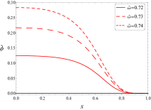
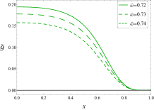
Figure 1: Scalar field function $\tilde{\phi}$(left panel) and Dirac field functions $\tilde{f}$(middle panel) and $\tilde{g}$(right panel) as functions of $x$ for $\tilde{\omega}=\tilde{\omega}_{S}=\tilde{\omega}_{D}=0.72,0.73,0.74$. All solutions have $\tilde{\mu}_{D}=0.95$ and $\tilde{\mu}_{S}=1$.

IV.1.1 One-Branch

The profiles of the field functions $\tilde{\phi}$, $\tilde{f}$ and $\tilde{g}$ with several values of synchronized frequency $\tilde{\omega}=\tilde{\omega}_{D}=\tilde{\omega}_{S}$ in the solutions of the $D_{0}S_{0}$ state are shown in Fig. 1. For the scalar field, as the frequency $\tilde{\omega}$ increases, $\tilde{\phi}_{max}$ (the maximum value of the field function $\tilde{\phi}$) increases. However, for the Dirac field, as the frequency $\tilde{\omega}$ increases, $\tilde{f}_{max}$ and $\tilde{g}_{max}$ (the maximum values of the field functions $\tilde{f}$ and $\tilde{g}$) decrease. Furthermore, we would like to study DBSs in the $D_{0}S_{0}$ state, where both the scalar and Dirac fields are in the ground state. It can be seen that there are no nodes in the matter functions in Fig. 1, which means that the scalar and Dirac fields are in the ground state.

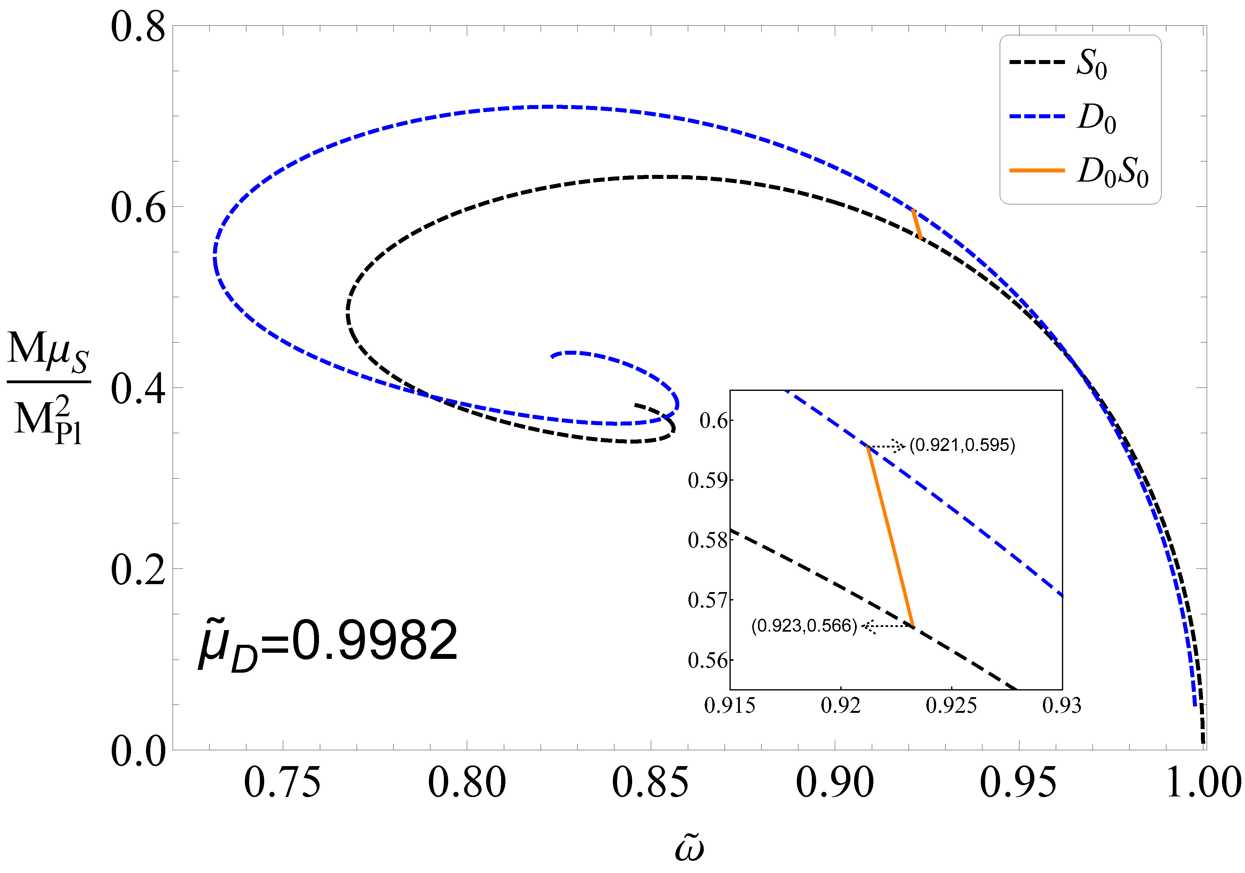
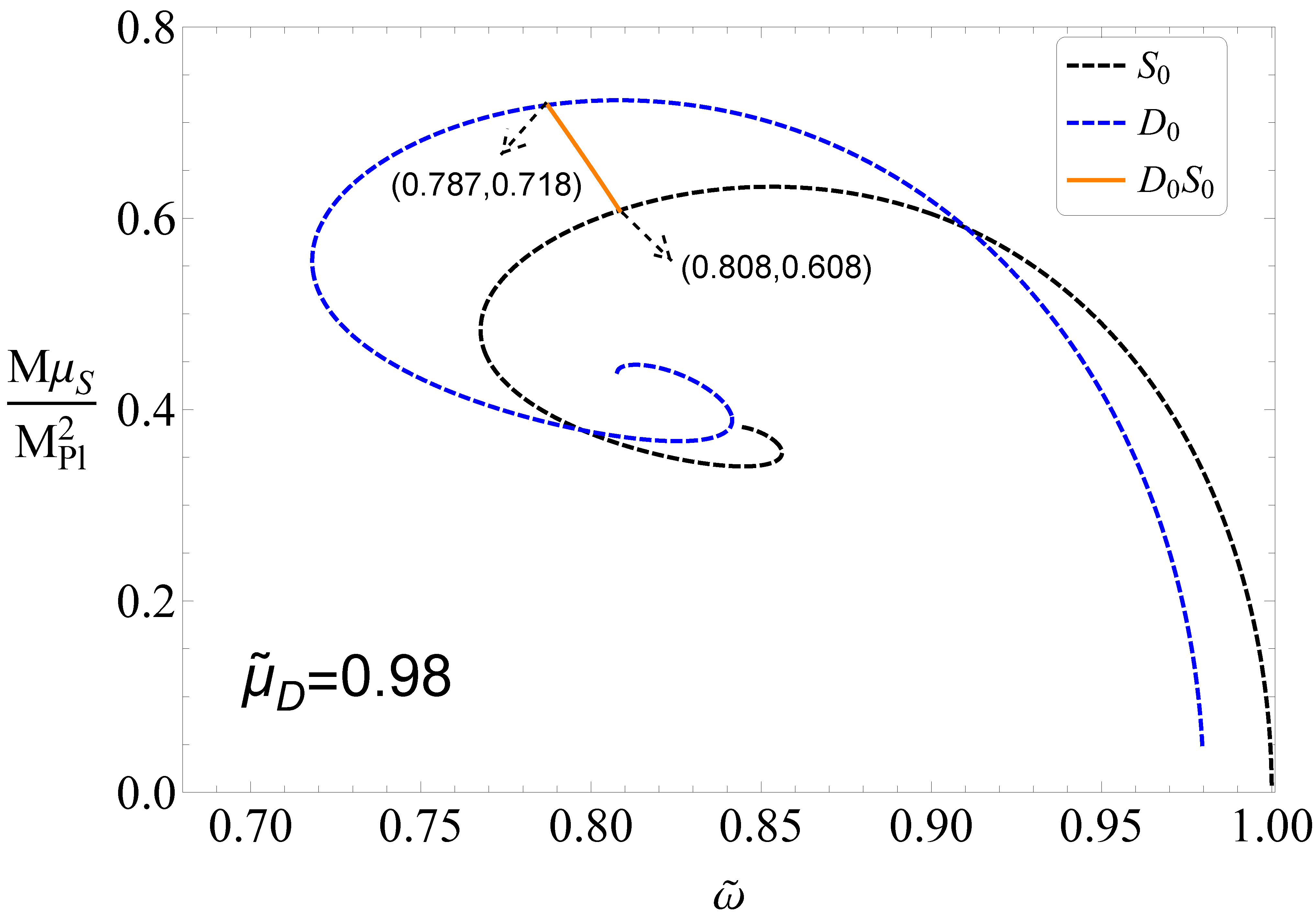
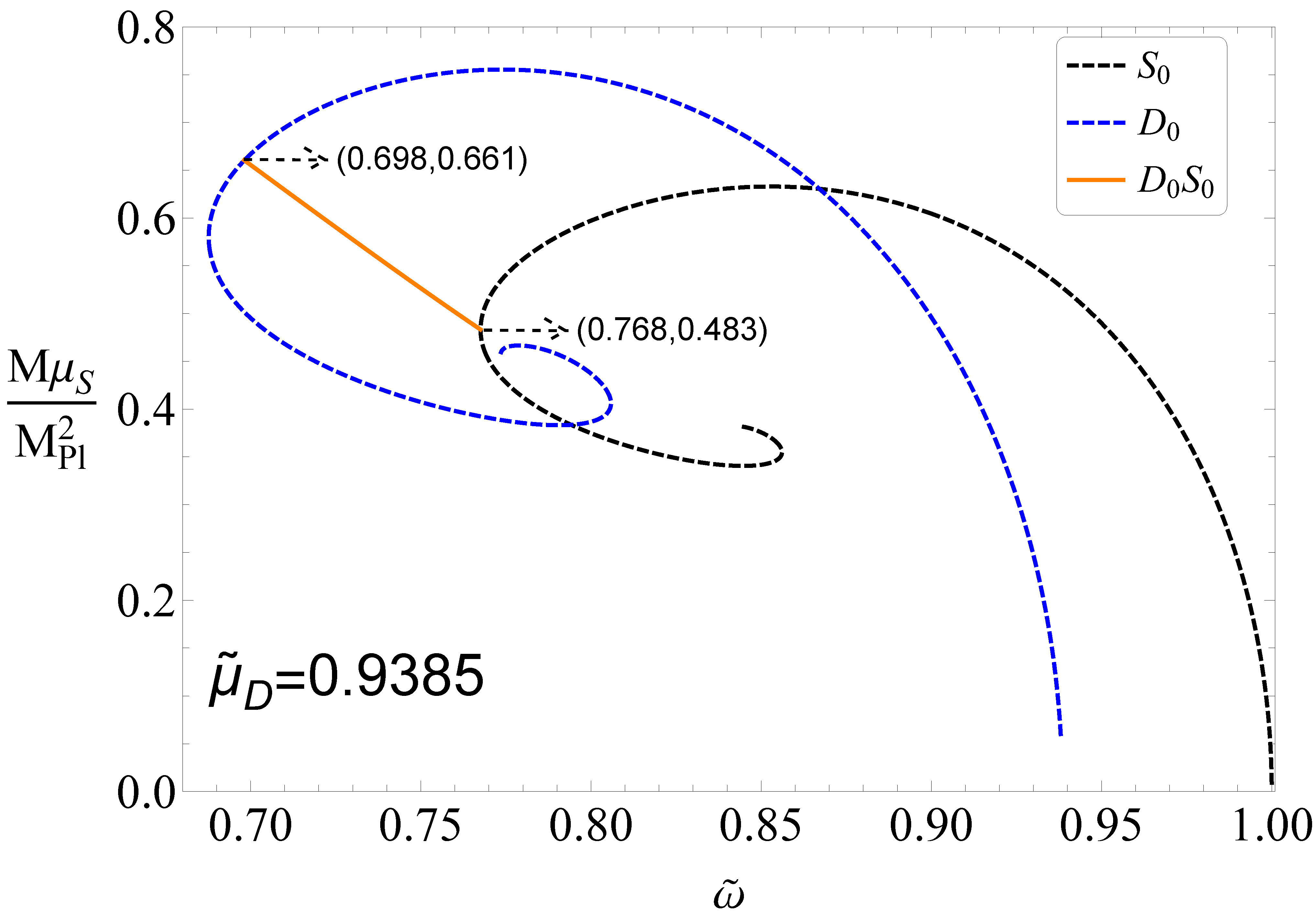
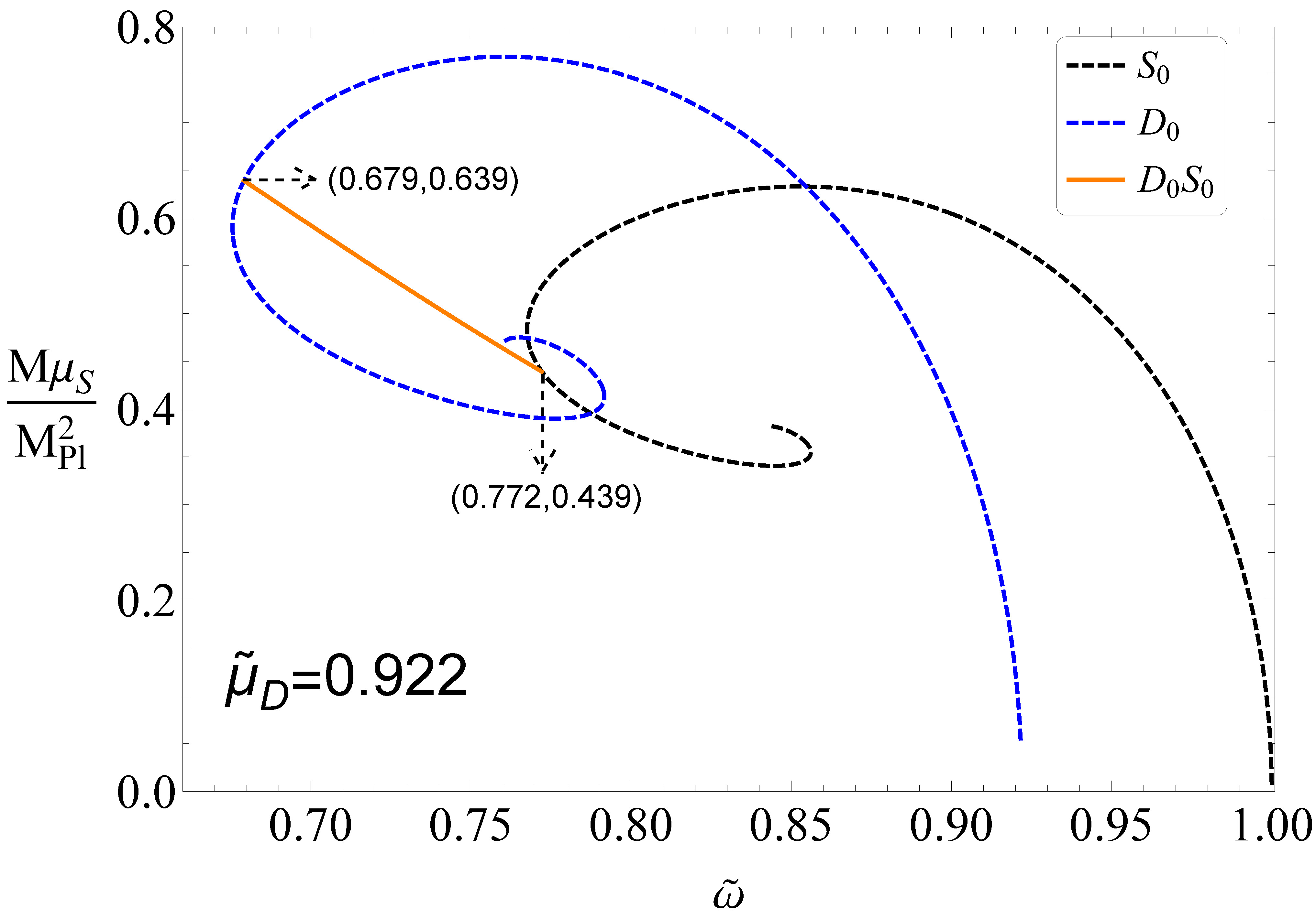
Figure 2: The ADM mass $M$ of the DBSs as a function of the synchronized frequency $\tilde{\omega}$ for $\tilde{\mu}_{D}=0.9982,0.98,0.96,0.9385,0.922,0.9051$. The black dashed line represents the $S_{0}$ state solutions with $\tilde{\mu}_{S}=1$, the blue dashed line represents the $D_{0}$ state solutions, and the orange line denote the coexisting state $D_{0}S_{0}$. All solutions have $\tilde{\mu}_{S}=1$.

The ADM mass $M$ of the DBSs versus the synchronized frequency $\tilde{\omega}$ for several values of the mass $\tilde{\mu}_{D}$ are presented in Fig. 2. The black dashed line represents the $S_{0}$ state solutions of the boson stars with $\tilde{\mu}_{S}=1$, the blue dashed line represents the $D_{0}$ state solutions of the Dirac stars, and the orange line denotes the coexisting state $D_{0}S_{0}$ of the DBSs. The relationship between the ADM mass of the DBSs and the synchronized frequency is similar to the case of the ${}^{1}S^{2}S$ or ${}^{1}S^{2}P$ of the RMSBSs in Ref. Li:2019mlk , the solutions of DBSs have only one branch. It can be seen that the mass $M$ of the DBSs decrease with increasing synchronized frequency $\tilde{\omega}$. The two ends of the orange line intersect with the blue and black dashed lines, respectively. We can see from Fig. 1 that the amplitude of the scalar field function $\tilde{\phi}$ increases with the increase of the synchronization frequency, and the amplitude of the Dirac field functions $\tilde{f}$ and $\tilde{g}$ decrease with the increase of the synchronization frequency. When the ADM mass $M$ of the DBSs reaches a maximum, the scalar field disappears, and the DBSs transform into Dirac stars, while when the ADM mass $M$ of the DBSs comes to a minimum, the Dirac fields disappear, and the DBSs transform into BSs.

In addition, when $\tilde{\mu}_{D}>0.9385$, the intersection of the orange line and the black dashed line is at the first branch of the black dashed line; when $\tilde{\mu}_{D}=0.9385$, the intersection is at the inflection point of the black dashed line; when $\tilde{\mu}_{D}<0.9385$, the intersection is at the black dashed line the second branch. And for $0.9051\leq\tilde{\mu}_{D}\leq 0.9982$, the intersection of the orange line and the blue dashed line is always in the first branch of the blue dashed line. It can be seen from the coordinates at both ends of the orange line marked in Fig. 2 that as the mass of the Dirac field decreases, the existence domain of the synchronized frequency gradually increases.

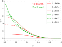
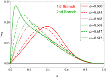
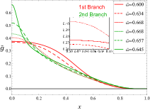
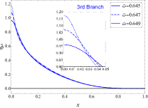
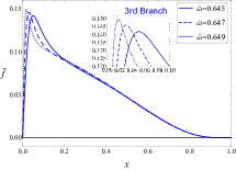
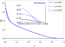
Figure 3: Scalar field function $\tilde{\phi}$(left panel) and Dirac field functions $\tilde{f}$(middle panel) and $\tilde{g}$(right panel) as functions of $x$ with several values of synchronized frequency $\tilde{\omega}$, where the field functions on the first, second and third branches are represented by the red, orange and blue lines. All solutions have $\tilde{\mu}_{D}=0.781$ and $\tilde{\mu}_{S}=1$.

IV.1.2 Multi-Branch

For the multi-branch solution family, the amplitudes of the field functions $\tilde{\psi}$, $\tilde{f}$ and $\tilde{g}$ on each branch with the synchronized frequency is shown in Fig. 3. The field functions on the first, second and third branches are represented by the red, orange and blue lines, respectively. For the first branch solutions, $\tilde{\psi}_{max}$ gradually increases as the synchronized frequency $\tilde{\omega}$ increases, while $\tilde{f}_{max}$ and $\tilde{g}_{max}$ first decrease and then increase. For the second branch solutions, $\tilde{\psi}_{max}$, $\tilde{f}_{max}$ and $\tilde{g}_{max}$ increase as the synchronized frequency $\tilde{\omega}$ decreases. For the third branch solutions, $\tilde{\psi}_{max}$, $\tilde{f}_{max}$ and $\tilde{g}_{max}$ decrease with increasing synchronized frequency.

It can be seen from Fig. 2 that when $\tilde{\mu}_{D}=0.9051$, the orange line is tangent to the second branch of the black dashed line. If we continue to reduce the mass $\tilde{\mu}_{D}$, we can get the solutions of DBSs with multiple branches. As shown in Fig. 4, we show the ADM mass $M$ of the DBSs versus the synchronized frequency $\tilde{\omega}$ for several values of the mass $\tilde{\mu}_{D}$ less than $0.9051$. The black dashed line is the same as in Fig. 2, and the blue dashed line represents the solutions of the $D_{0}$ state when $\tilde{\mu}_{D}$ takes the value marked in the figure. Each orange line has multiple branches, and the whole line is a spiral, the variation of the mass $M$ of the DBSs with the synchronized frequency is more complicated than that in Fig. 2. For any solution on the orange line, the amplitude of the Dirac field in the corresponding solution is always not zero. In other words, there is no solution similar to the intersection of the orange line and the black dashed line in Fig. 2. When $\tilde{\mu}_{D}>0.894$, the intersection of the orange line and the blue dashed line (the point with the coordinates marked in Fig. 4) is located on the first branch of the blue dashed line; when $\tilde{\mu}_{D}=0.894$, the intersection is precisely at the inflection point of the blue dashed line; when $0.559\leq\tilde{\mu}_{D}<0.894$, the intersection is on the second branch of the blue dashed line.

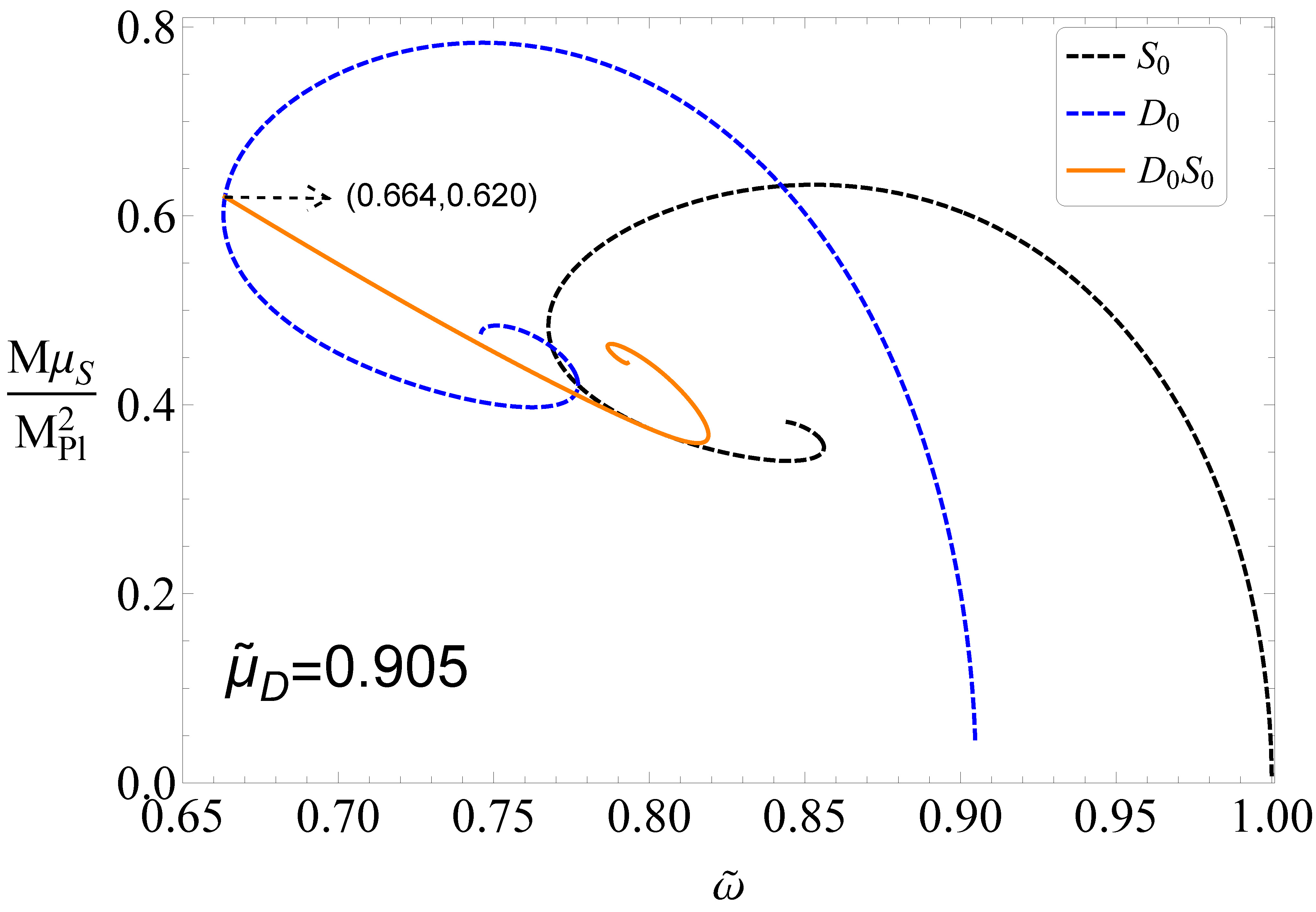
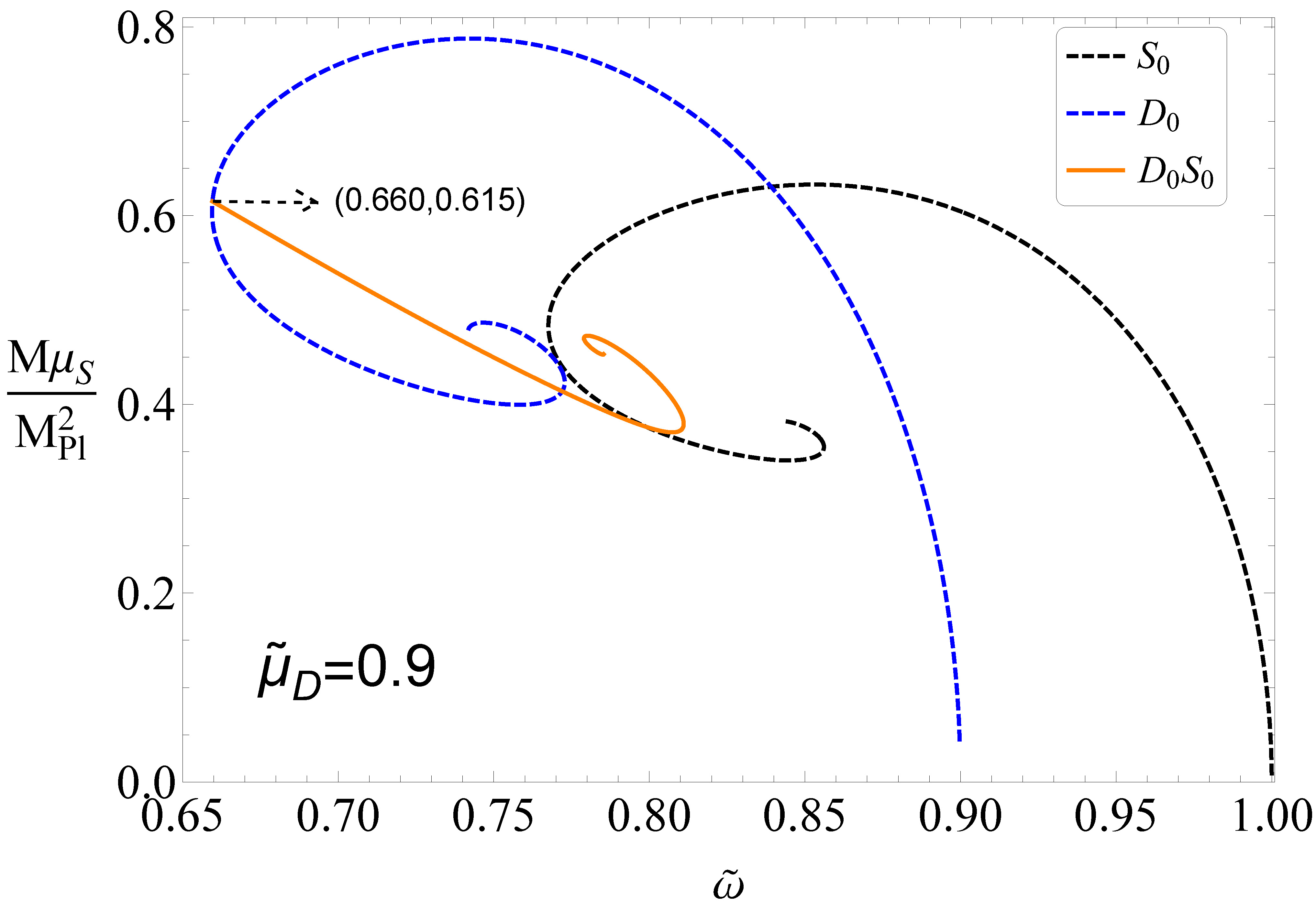
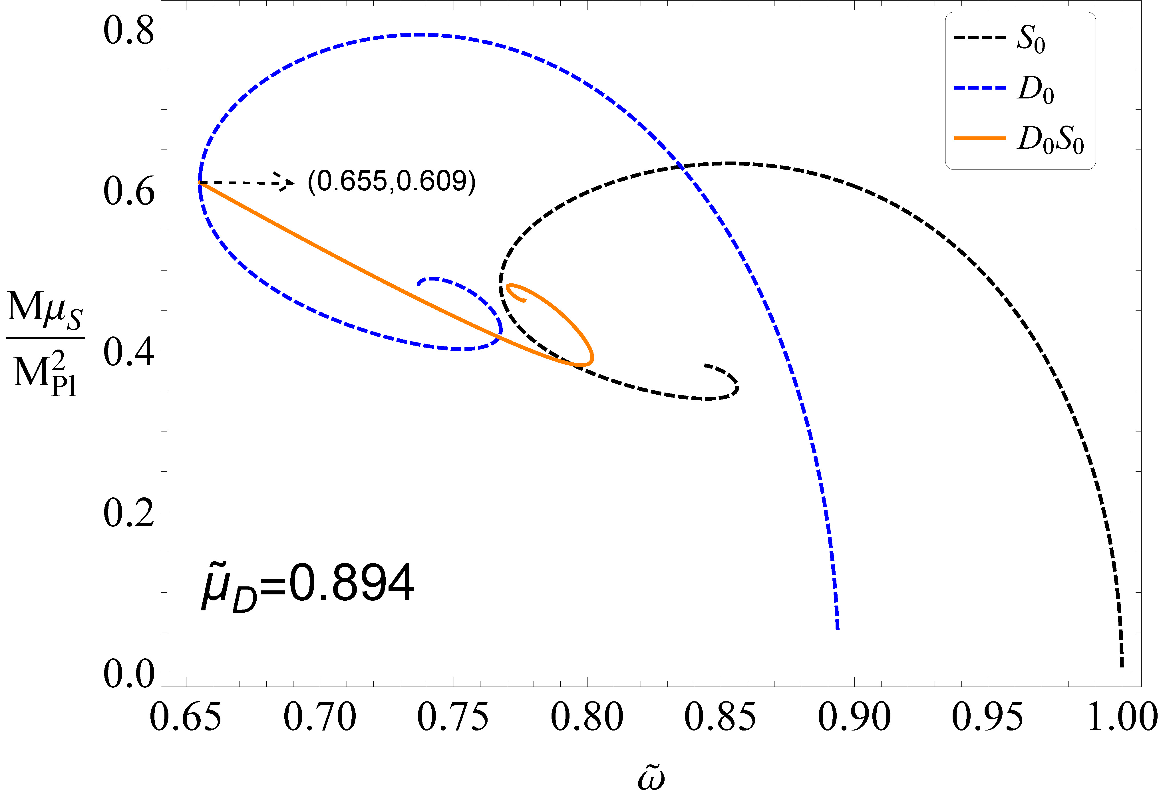
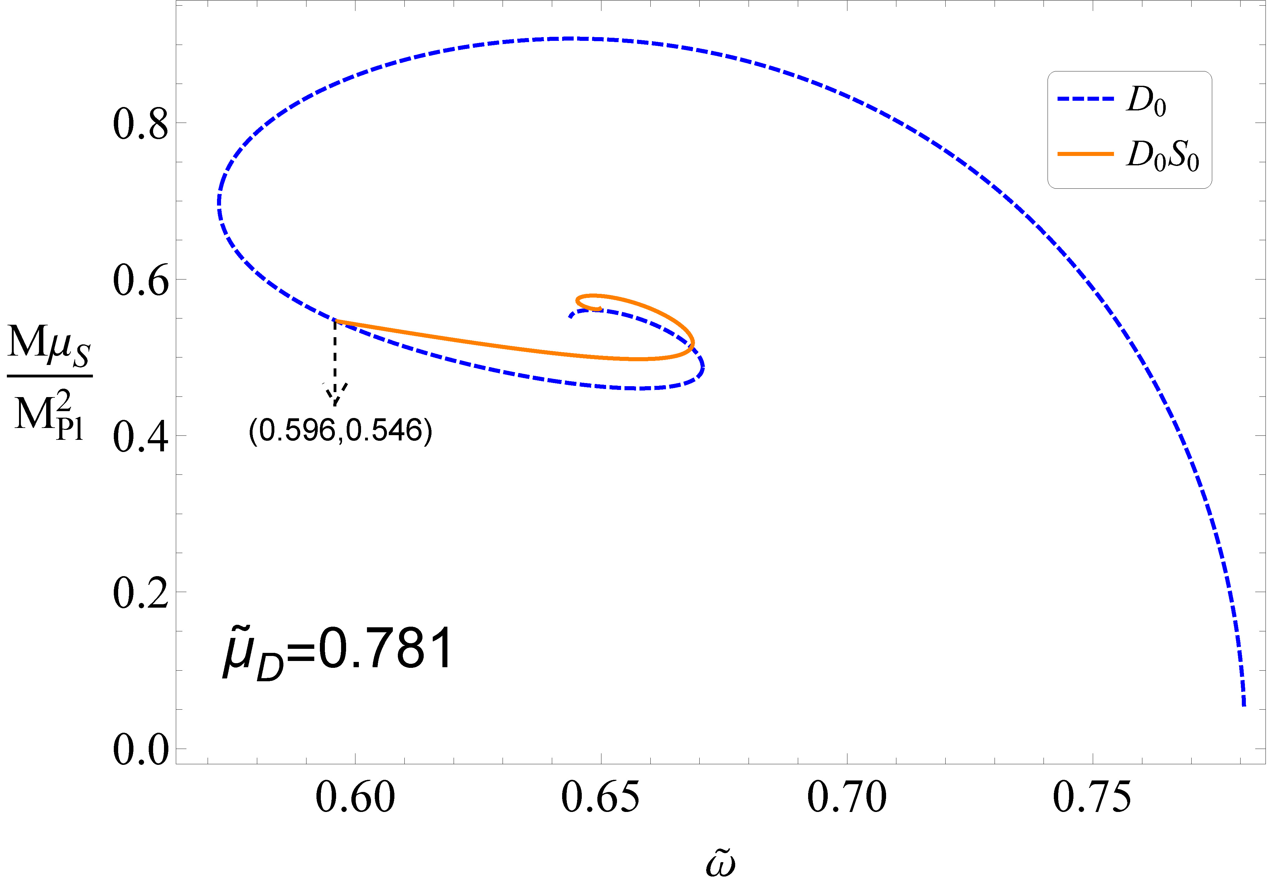
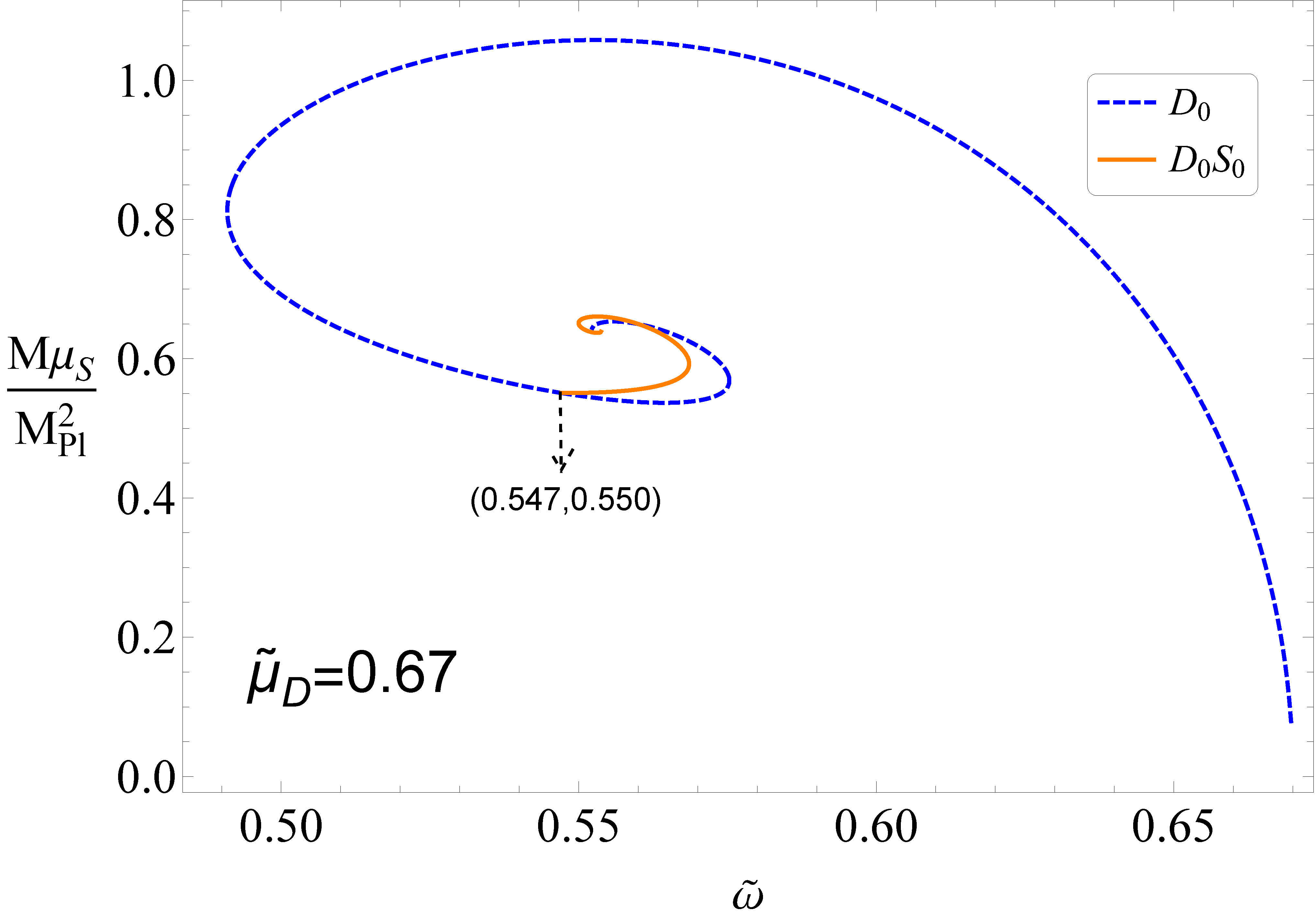
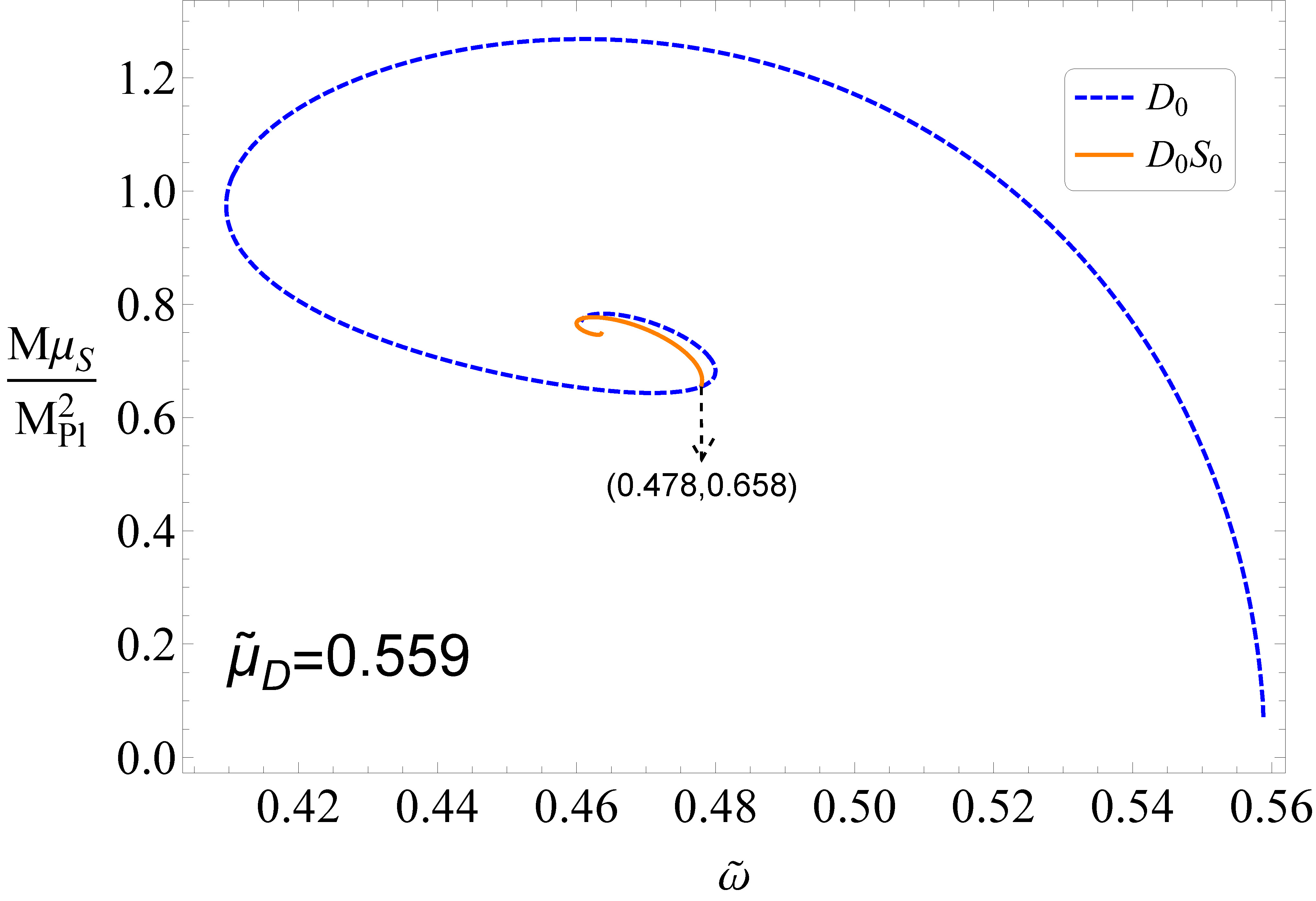
Figure 4: The ADM mass $M$ of the DBSs as a function of the synchronized frequency $\tilde{\omega}$ for $\tilde{\mu}_{D}=0.905,0.9,0.894,0.781,0.67,0.559$. The black dashed line represents the $S_{0}$ state solutions with $\tilde{\mu}_{S}=1$, the blue dashed line represents the $D_{0}$ state solutions, and the orange line denote the coexisting state $D_{0}S_{0}$. All solutions have $\tilde{\mu}_{S}=1$.

In Table 1, we show the existence domain of the synchronized frequency $\tilde{\omega}$ for several values of the Dirac field mass $\tilde{\mu}_{D}$. As the Dirac field mass $\tilde{\mu}_{D}$ decreases, the intervals of $B_{1}$, $B_{2}$ and $B_{3}$ are gradually narrowed. When $\tilde{\mu}_{D}$ decreases to $0.559$, the interval of $B_{1}$ becomes very narrow; while the interval of $B_{2}$ and $B_{3}$ change relatively little. Moreover, as the Dirac field mass $\tilde{\mu}_{D}$ decreases, $M_{max}$ first decreases and then increases, while $M_{min}$ keeps increasing.

$\tilde{\mu}_{D}$	$B_{1}$	$B_{2}$	$B_{3}$	$M_{max}$	$M_{min}$
$0.905$	$0.664\sim 0.819$	$0.787\sim 0.819$	$0.787\sim 0.793$	$0.620$	$0.359$
$0.900$	$0.660\sim 0.811$	$0.779\sim 0.811$	$0.779\sim 0.785$	$0.615$	$0.370$
$0.894$	$0.655\sim 0.802$	$0.770\sim 0.802$	$0.770\sim 0.776$	$0.609$	$0.382$
$0.781$	$0.596\sim 0.669$	$0.645\sim 0.669$	$0.645\sim 0.650$	$0.579$	$0.498$
$0.670$	$0.547\sim 0.569$	$0.550\sim 0.569$	$0.550\sim 0.554$	$0.661$	$0.551$
$0.559$	$0.4780\sim 0.4781$	$0.460\sim 0.478$	$0.460\sim 0.464$	$0.777$	$0.658$

Table 1: Maximum and minimum ADM masses($M_{max}$ and $M_{min}$) of the DBSs, and the existence domain of the synchronized frequency $\tilde{\omega}$ for several values of the Dirac field mass $\tilde{\mu}_{D}$. $B_{1}$, $B_{2}$ and $B_{3}$ represent the first, second and third branches of the orange line in Fig. 4, respectively. All solutions have $\tilde{\mu}_{S}=1$.

IV.2 Nonsynchronized frequency

Similar to the case of synchronized frequency, we divide the families of nonsynchronized frequency solutions of DBSs into three categories: the one-branch-A solution family, multi-branch solution family, and one-branch-B solution family. The value ranges of $\tilde{\omega}_{S}$ corresponding to these three solution families are $0.7676\leq\tilde{\omega}_{S}\leq 0.9082$, $0.7128\leq\tilde{\omega}_{S}\leq 0.7675$ and $0.6794\leq\tilde{\omega}_{S}\leq 0.7127$, respectively. The remainder of this section discusses these three families of solutions in detail.

IV.2.1 One-Branch-A

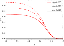
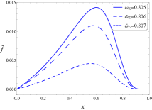
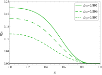
Figure 5: Scalar field function $\tilde{\phi}$(left panel) and Dirac field functions $\tilde{f}$(middle panel) and $\tilde{g}$(right panel) as functions of $x$ with $\tilde{\omega}_{D}=0.805,0.806,0.807$. All solutions have $\tilde{\omega}_{S}=0.79$ and $\tilde{\mu}_{S}=\tilde{\mu}_{D}=1$.

For one-branch-A solution families, the profiles of the field functions $\tilde{\phi}$, $\tilde{f}$ and $\tilde{g}$ with several values of the nonsynchronized frequency $\tilde{\omega}_{D}$ in the solutions of the $D_{0}S_{0}$ state are shown in Fig. 5. Similar to the case in Fig. 1, as the nonsynchronized frequency $\tilde{\omega}_{D}$ increases, $\tilde{\phi}_{max}$ increases and $\tilde{f}_{max}$ and $\tilde{g}_{max}$ decreases.

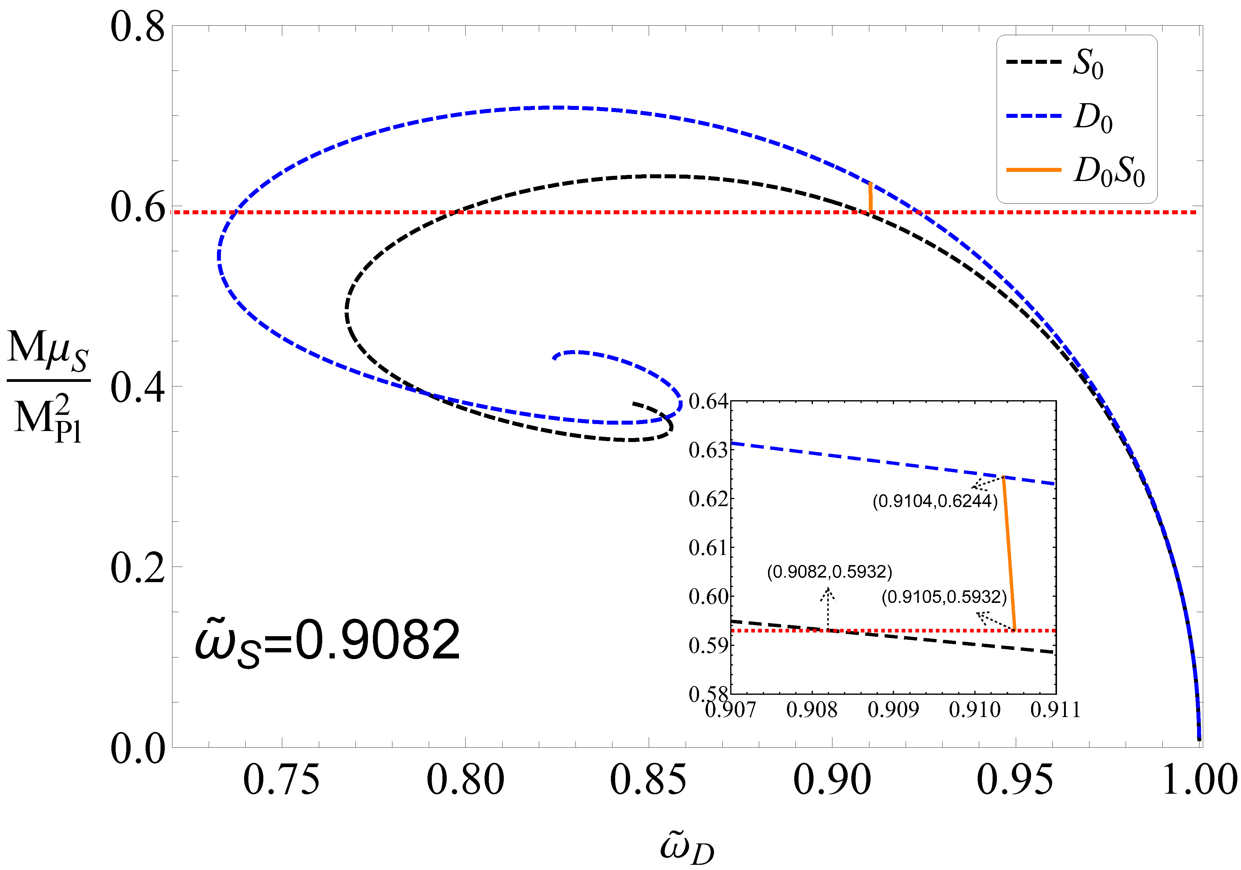
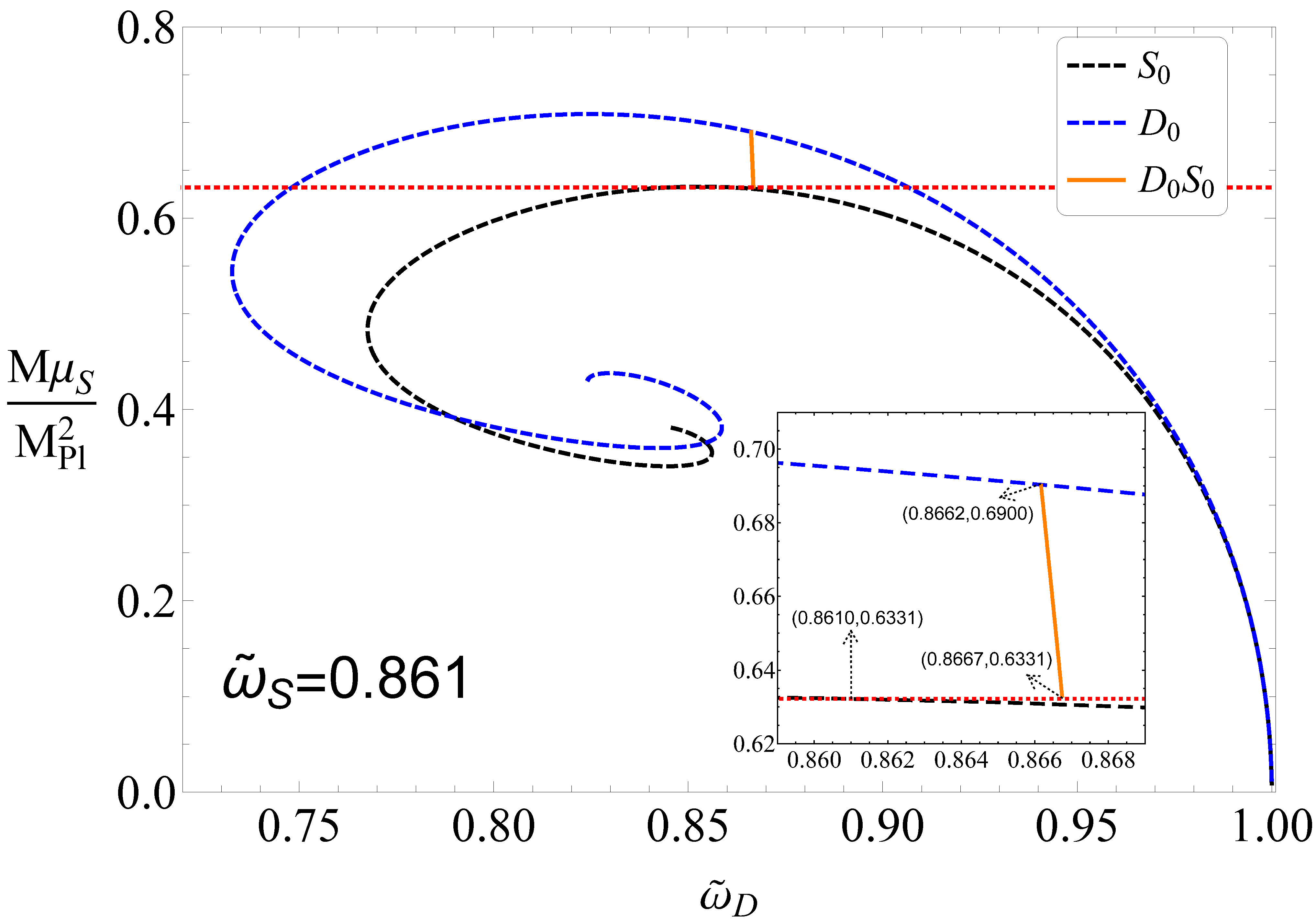
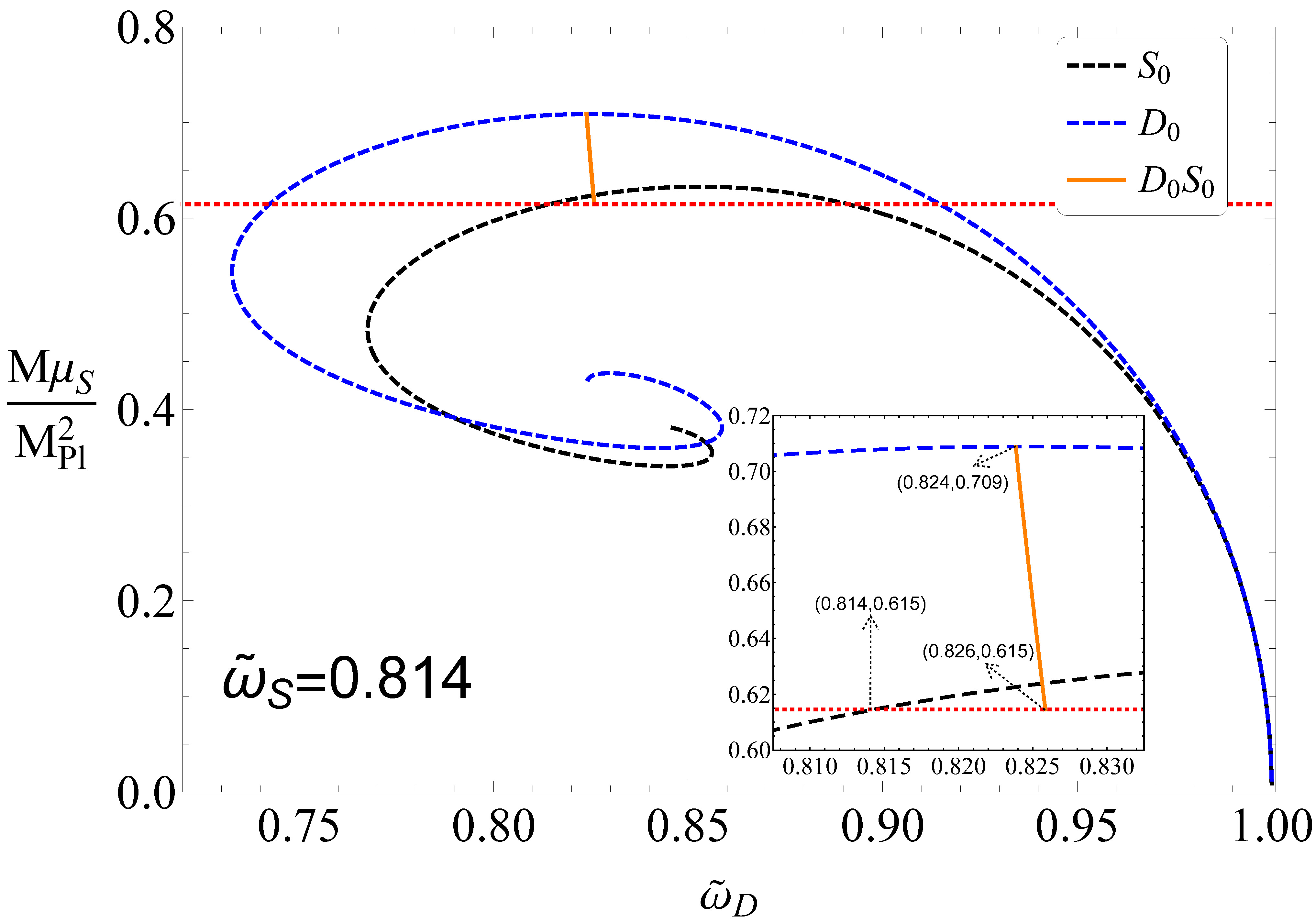
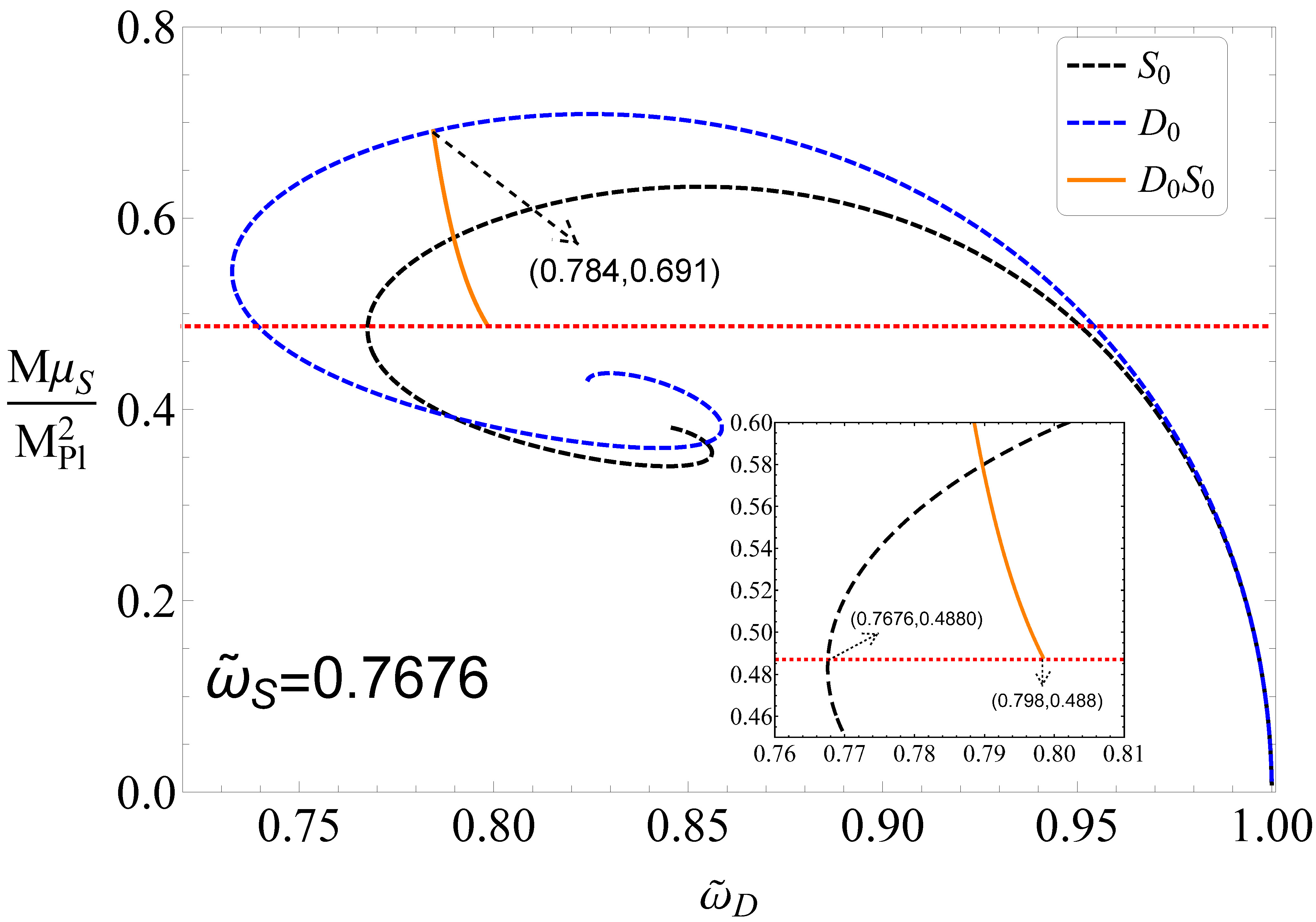
Figure 6: The ADM mass $M$ of the DBSs as a function of the nonsynchronized frequency $\tilde{\omega}_{D}$ for $\tilde{\omega}_{S}=0.9082,0.861,0.814,0.7676$. The black dashed line represents the $S_{0}$ state solutions, the blue dashed line represents the $D_{0}$ state solutions, the red horizontal dashed line represents the ADM mass of the BSs with $S_{0}$ state when $\tilde{\omega}_{S}$ takes the value marked in the figure, and the orange line denote the coexisting state $D_{0}S_{0}$. All solutions have $\tilde{\mu}_{D}=\tilde{\mu}_{S}=1$.

In Fig. 6, we show the ADM mass $M$ of the DBSs versus the nonsynchronized frequency $\tilde{\omega}_{D}$ for several values of the scalar field frequency $\tilde{\mu}_{S}$, where $0.7676\leq\tilde{\mu}_{S}\leq 0.9082$. The black and blue dashed lines represent the solutions of $S_{0}$ and $D_{0}$, and the orange line represents the DBSs. As can be seen from the insets in each panel, as the scalar field frequency $\tilde{\omega}_{S}$ decreases, the existence domain of the nonsynchronized frequency $\tilde{\omega}_{D}$ increases. In addition, the ADM mass $M$ of the DBSs decreased with increasing $\tilde{\omega}_{D}$. Similar to Fig. 2, when the ADM mass $M$ of the DBSs reaches a maximum, the scalar field disappears, and the DBSs transform into Dirac stars, while when the ADM mass $M$ of the DBSs comes to a minimum, the Dirac fields disappear, and the DBSs transform into BSs. The ADM mass of the BSs is equal to the minimum of the ADM mass of the DBSs when the scalar field frequency $\tilde{\mu}_{S}$ is taken at the value marked in each panel. In other words, for the one-branch-A solution families, the minimum value of the ADM mass $M$ of the DBSs depends on the scalar field frequency $\tilde{\omega}_{S}$.

IV.2.2 Multi-Branch

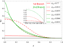
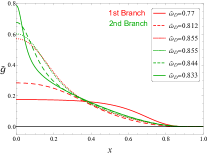
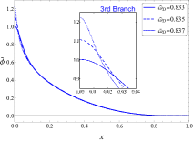
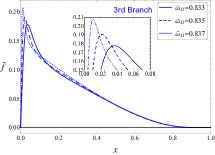
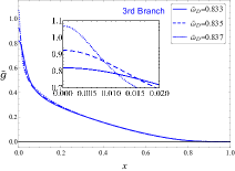
Figure 7: Scalar field function $\tilde{\phi}$(left panel) and Dirac field functions $\tilde{f}$(middle panel) and $\tilde{g}$(right panel) as functions of $x$ with several values of nonsynchronized frequency $\tilde{\omega}_{D}$, where the field functions on the first, second and third branches are represented by the red, orange and blue lines. All solutions have $\tilde{\omega}_{S}=0.749$ and $\tilde{\mu}_{S}=\tilde{\mu}_{D}=1$.

For multi-branch solution families, the change of the field functions $\tilde{\psi}$, $\tilde{f}$ and $\tilde{g}$ on each branch with the nonsynchronized frequency $\tilde{\omega}_{D}$ is shown in Fig. 7. The field functions on the first, second and third branches are represented by the red, orange and blue lines, respectively. For the first and third branch solutions, $\tilde{\psi}_{max}$, $\tilde{f}_{max}$ and $\tilde{g}_{max}$ gradually increase as the nonsynchronized frequency $\tilde{\omega}_{D}$ increases. For the second branch solutions, $\tilde{\psi}_{max}$, $\tilde{f}_{max}$ and $\tilde{g}_{max}$ increase as the nonsynchronized frequency $\tilde{\omega}_{D}$ decreases.

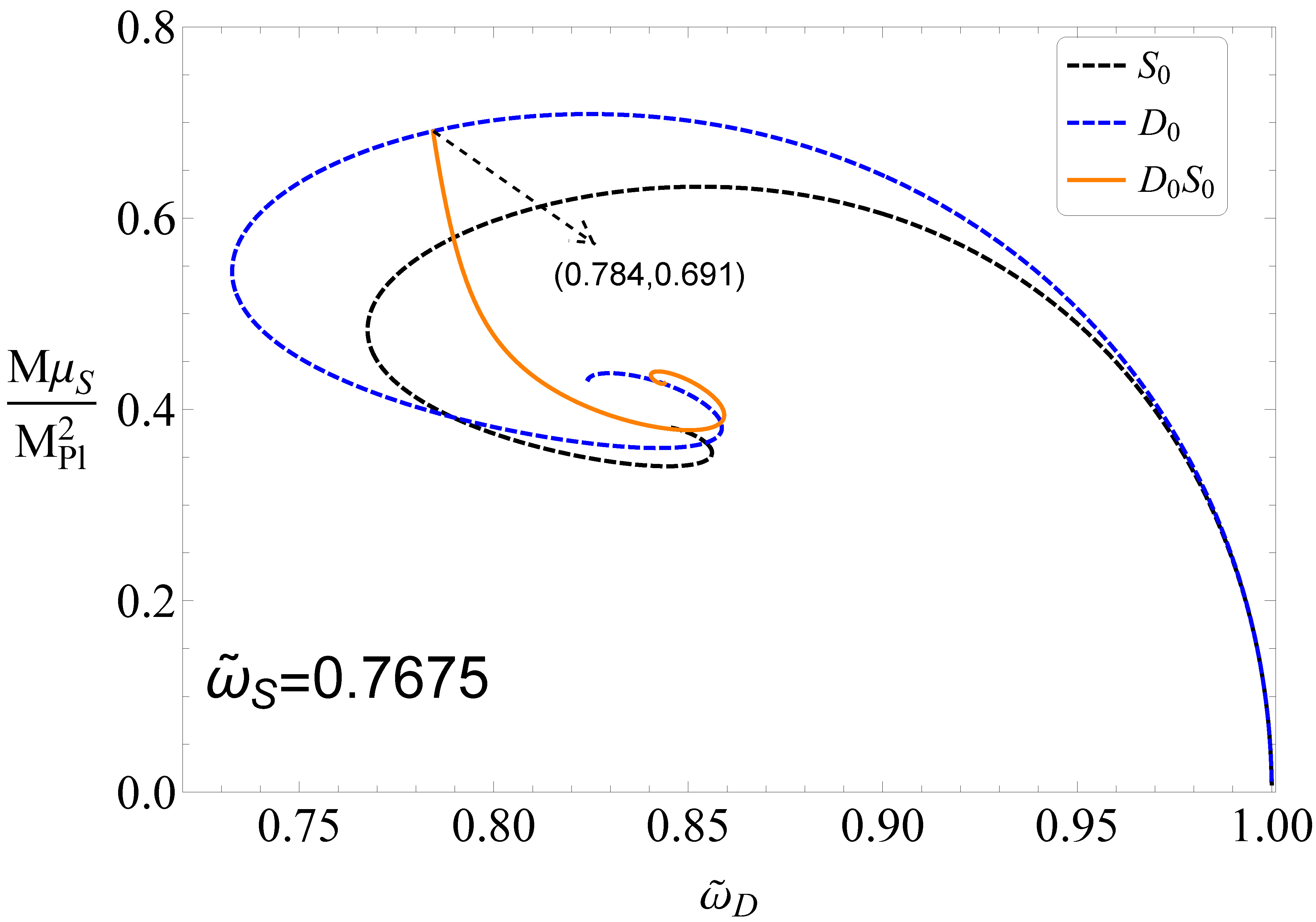
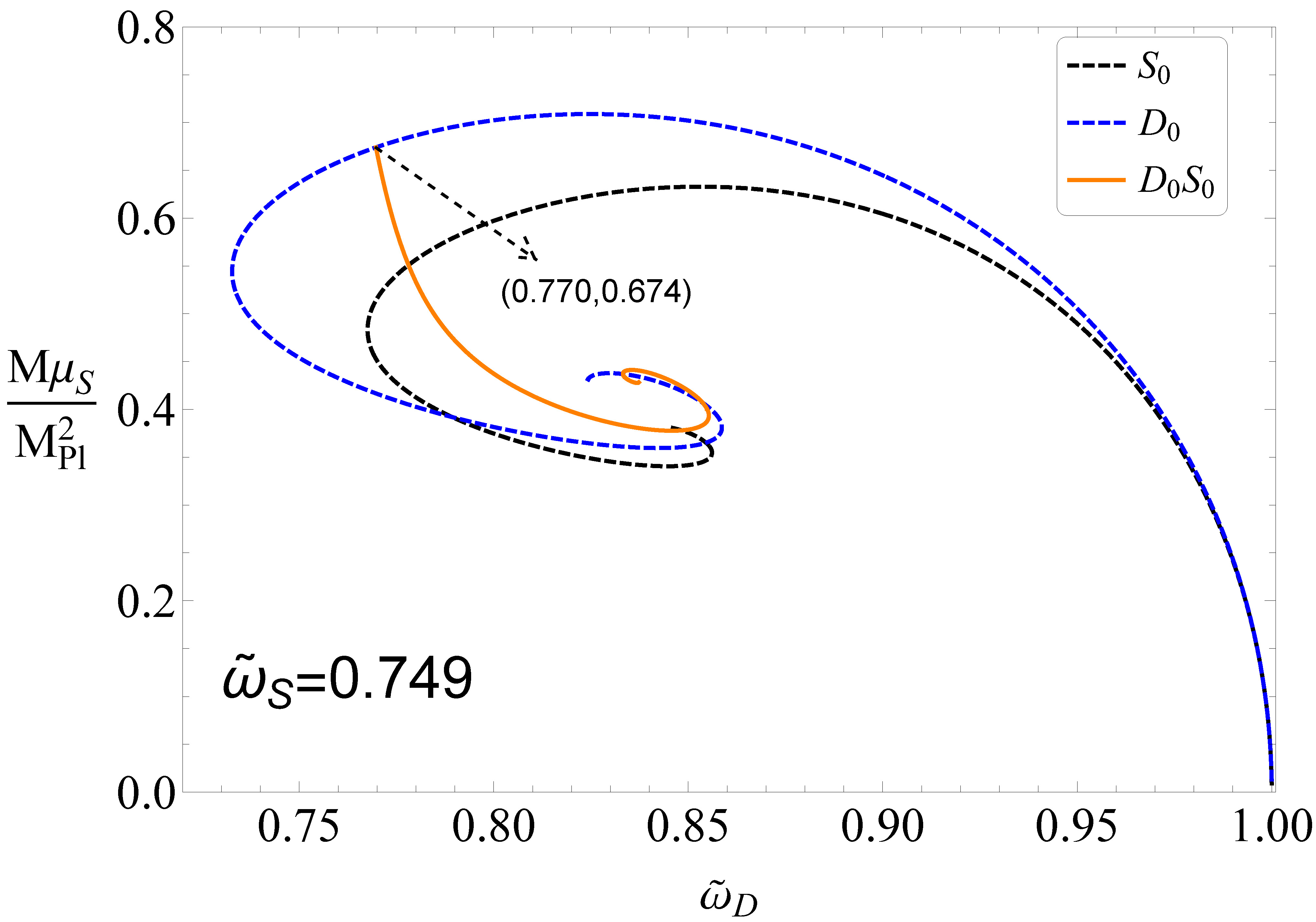
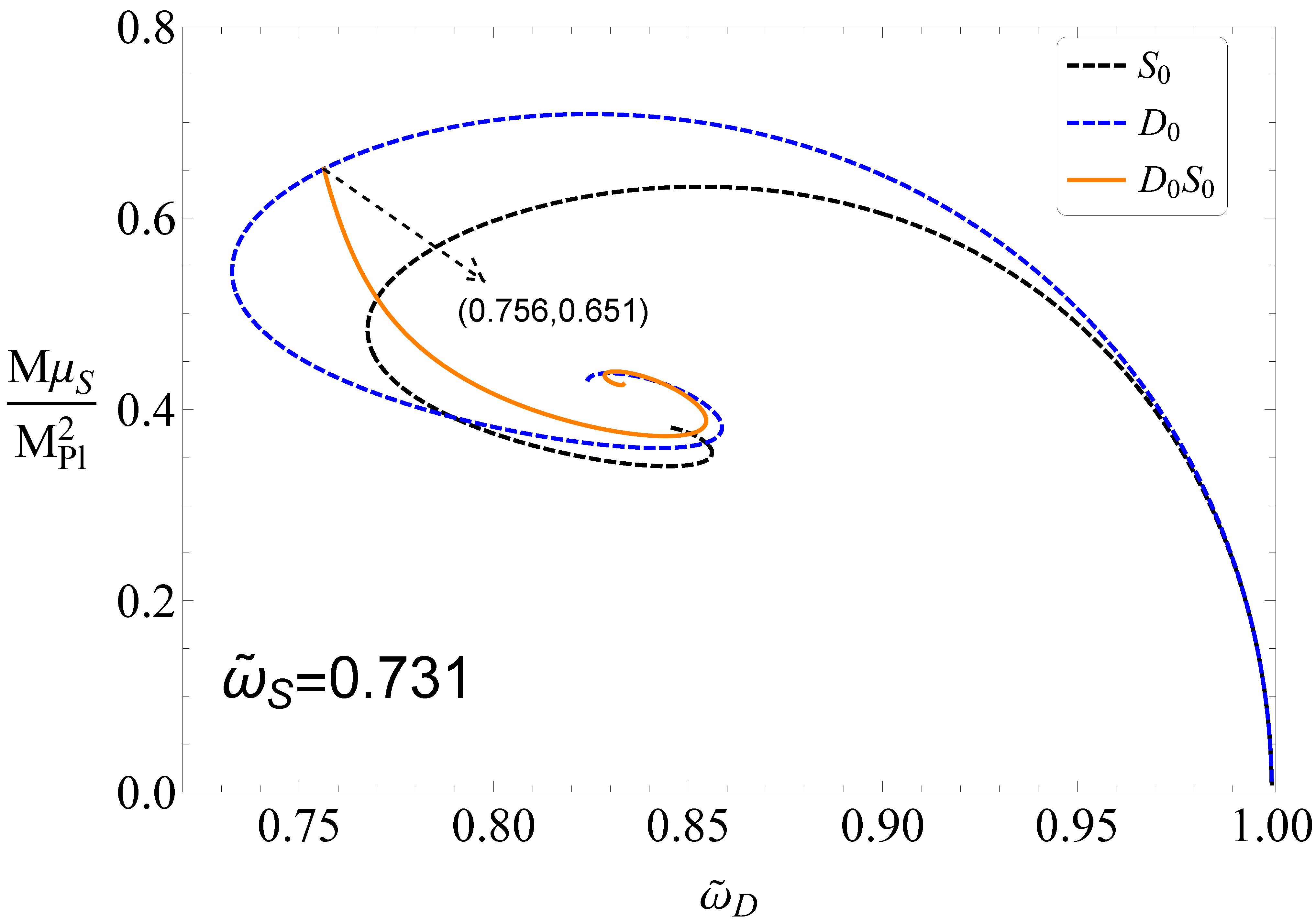
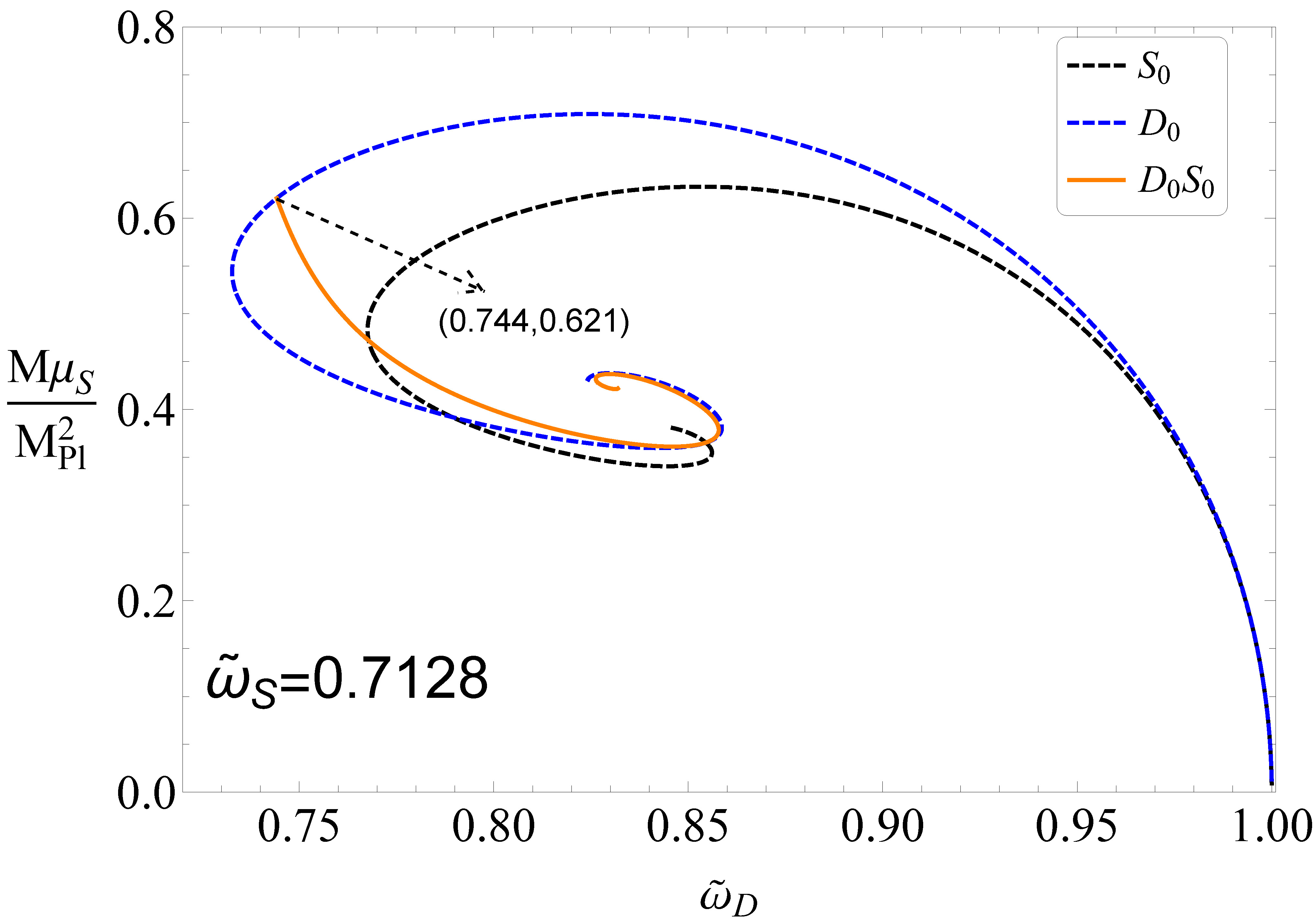
Figure 8: The ADM mass $M$ of the DBSs as a function of the nonsynchronized frequency $\tilde{\omega}_{D}$ for $\tilde{\omega}_{S}=0.7675,0.749,0.731,0.7128$. The black dashed line represents the $S_{0}$ state solutions, the blue dashed line represents the $D_{0}$ state solutions, and the orange line denote the coexisting state $D_{0}S_{0}$. All solutions have $\tilde{\mu}_{D}=\tilde{\mu}_{S}=1$.

$\tilde{\omega}_{S}$	$B_{1}$	$B_{2}$	$B_{3}$	$M_{max}$	$M_{min}$
$0.7675$	$0.784\sim 0.859$	$0.840\sim 0.859$	$0.840\sim 0.844$	$0.691$	$0.378$
$0.749$	$0.770\sim 0.855$	$0.833\sim 0.855$	$0.833\sim 0.837$	$0.674$	$0.378$
$0.731$	$0.756\sim 0.855$	$0.829\sim 0.855$	$0.829\sim 0.833$	$0.651$	$0.372$
$0.7128$	$0.744\sim 0.858$	$0.826\sim 0.858$	$0.826\sim 0.832$	$0.621$	$0.361$

Table 2: Maximum and minimum ADM masses($M_{max}$ and $M_{min}$) of the DBSs, and the existence domain of the nonsynchronized frequency $\tilde{\omega}_{D}$ for $\tilde{\omega}_{S}=0.7675,0.749,0.731,0.7128$. $B_{1}$, $B_{2}$ and $B_{3}$ represent the first, second and third branches of the orange line in Fig. 8, respectively. All solutions have $\tilde{\mu}_{S}=\tilde{\mu}_{D}=1$.

In Fig. 8, we show the ADM mass $M$ of the DBSs versus the nonsynchronized frequency $\tilde{\omega}_{D}$ for several values of the scalar field frequency $\tilde{\mu}_{S}$, where $0.7128\leq\tilde{\mu}_{S}\leq 0.7675$. The black dashed and blue dashed lines are the same as in Fig. 6. Like Fig. 4, each orange line has multiple branches, and the whole line is a spiral. At the intersection of the orange line and the blue dashed line, the DBSs transform into Dirac stars. For the other solutions on the orange line, both the scalar and Dirac fields coexist. Moreover, there is no solution on the orange line where the Dirac field functions vanish, i.e., there is no solution similar to the intersection of the black dashed line and the orange line in Fig. 2). In addition, unlike Fig. 4, the intersection of the orange line and the blue dashed line is always in the first branch of the blue dashed line.

In Table 2, we show the existence domain of the nonsynchronized frequency $\tilde{\omega}_{D}$ for several values of the scalar field frequency $\tilde{\omega}_{S}$. As the frequency $\tilde{\omega}_{S}$ decreases, the intervals of $B_{1}$, $B_{2}$ and $B_{3}$ are gradually narrowed, where the change in the intervals of $B_{3}$ is relatively small. Moreover, as the frequency $\tilde{\omega}_{S}$ decreases, both $M_{max}$ and $M_{min}$ gradually decrease.

IV.2.3 One-Branch-B

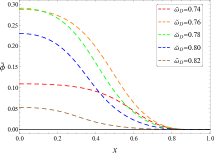
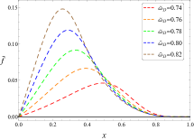
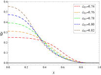
Figure 9: Scalar field function $\tilde{\phi}$(left panel) and Dirac field functions $\tilde{f}$(middle panel) and $\tilde{g}$(right panel) as functions of $x$ with $\tilde{\omega}_{D}=0.74,0.76,0.78,0.80,0.82$. All solutions have $\tilde{\omega}_{S}=0.702$ and $\tilde{\mu}_{S}=\tilde{\mu}_{D}=1$.

For one-branch-B solution families, the profiles of the field functions $\tilde{\phi}$, $\tilde{f}$ and $\tilde{g}$ with several values of nonsynchronized frequency $\tilde{\omega}_{D}$ in the solutions of the $D_{0}S_{0}$ state are shown in Fig. 9. For the scalar field, $\tilde{\phi}_{max}$ first increases and then decreases with the increase of the nonsynchronized frequency $\tilde{\omega}_{D}$. Whereas for Dirac field, $\tilde{f}_{max}$ and $\tilde{g}_{max}$ increase with increasing the frequency $\tilde{\omega}_{D}$.

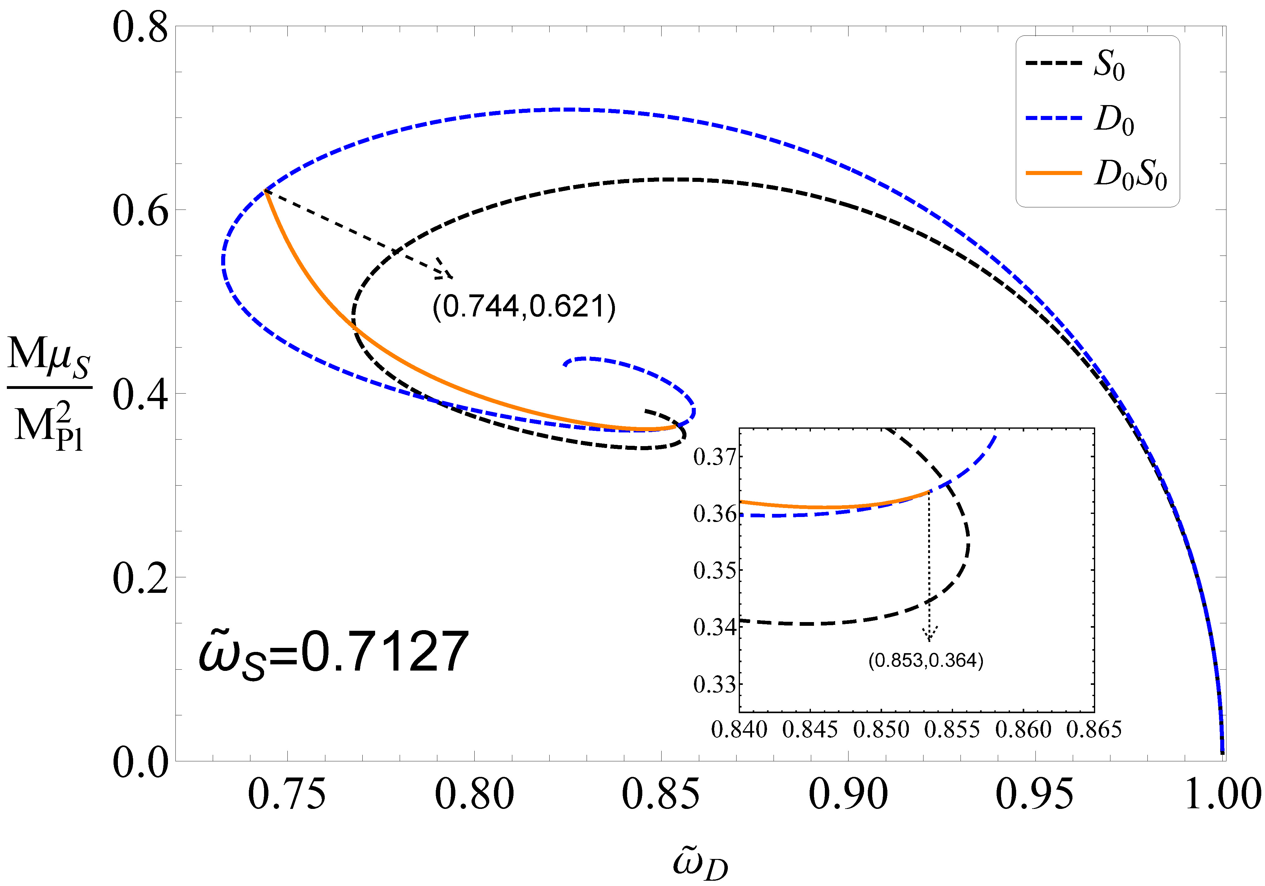
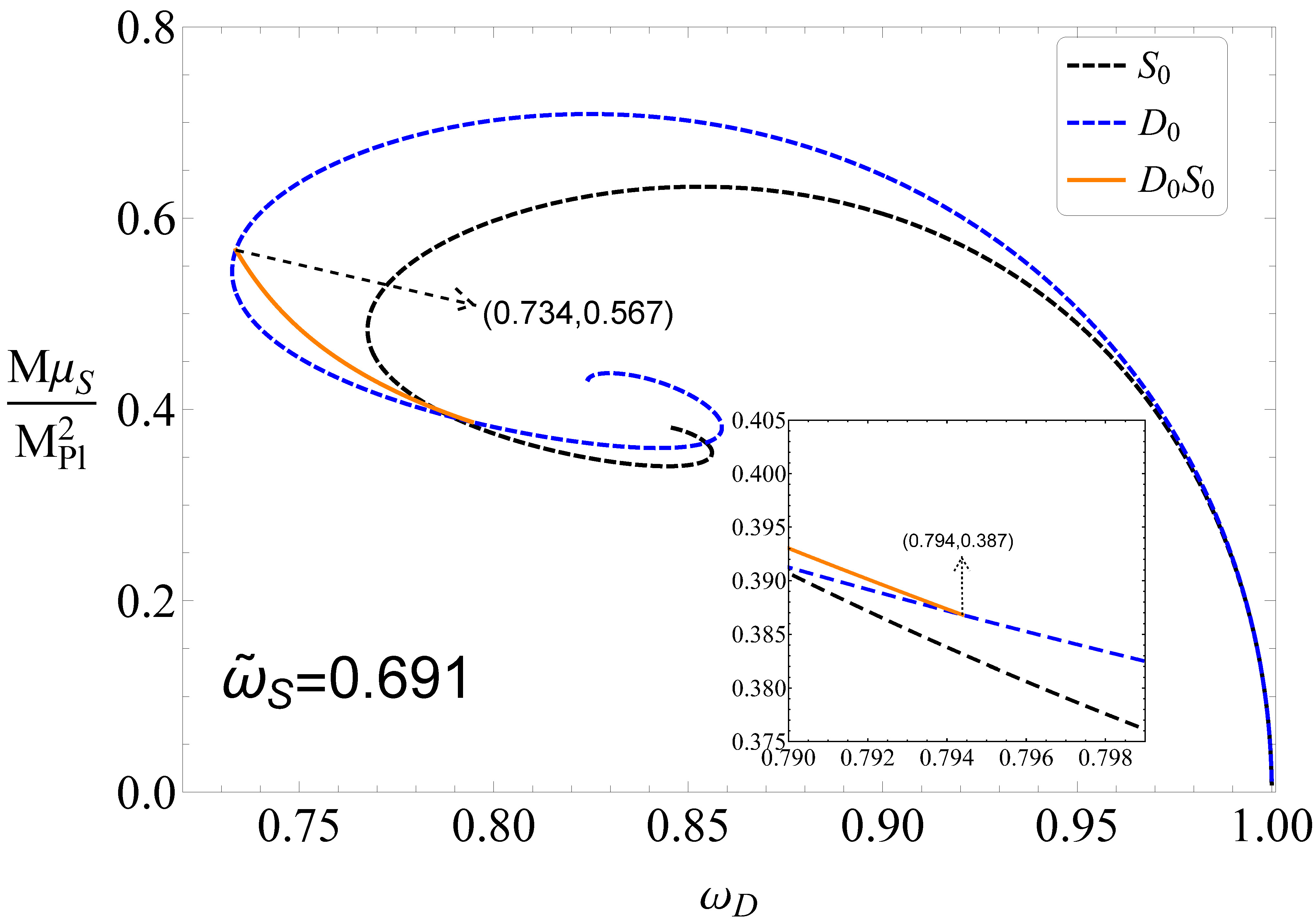
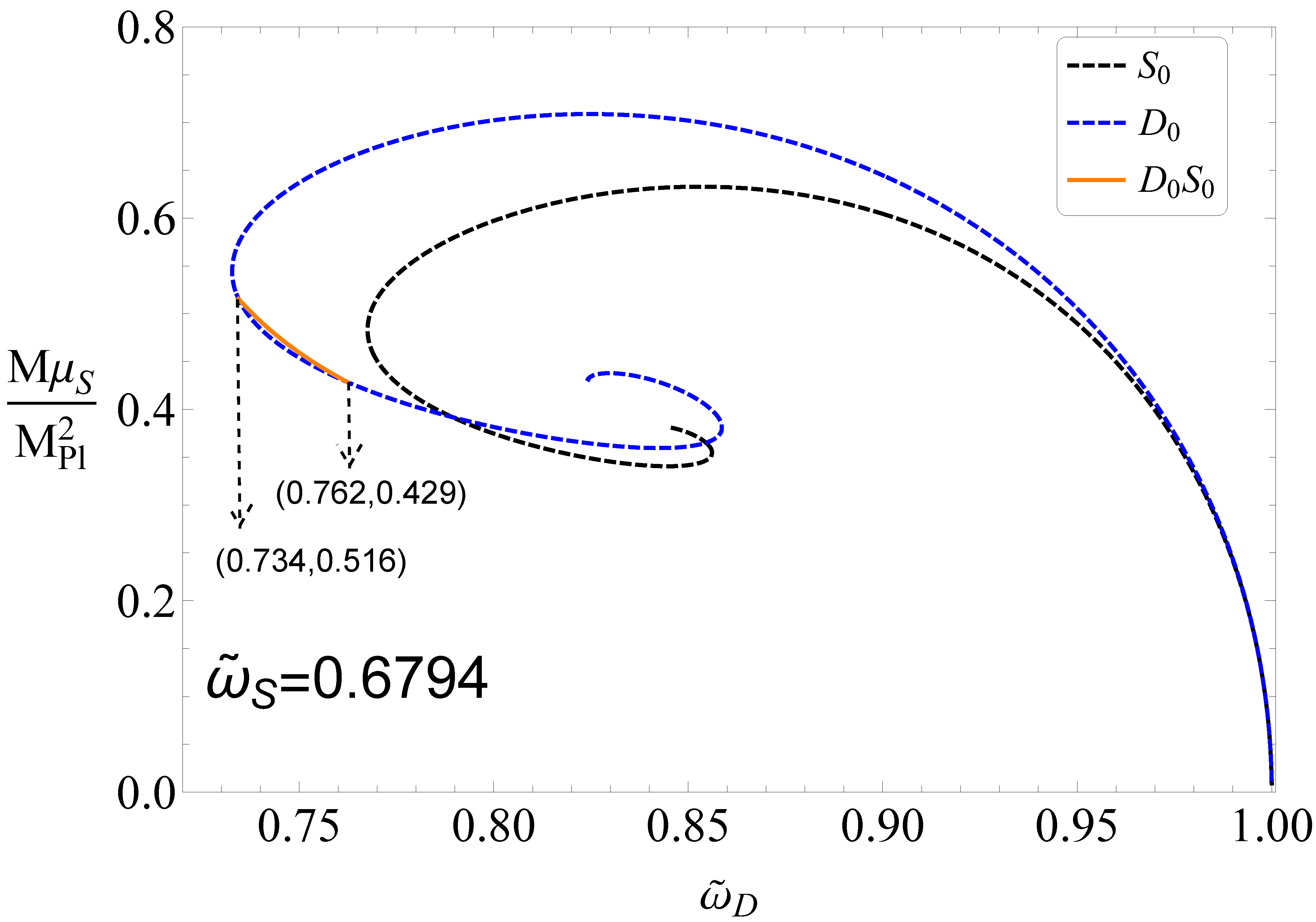
Figure 10: The ADM mass $M$ of the DBSs as a function of the nonsynchronized frequency $\tilde{\omega}_{D}$ for $\tilde{\omega}_{S}=0.7127,0.702,0.691,0.6794$. The black dashed line represents the $S_{0}$ state solutions, the blue dashed line represents the $D_{0}$ state solutions, and the orange line denote the coexisting state $D_{0}S_{0}$. All solutions have $\tilde{\mu}_{D}=\tilde{\mu}_{S}=1$.

In Fig. 10, we show the ADM mass $M$ of the DBSs versus the nonsynchronized frequency $\tilde{\omega}_{D}$ for several values of the scalar field frequency $\tilde{\mu}_{S}$, where $0.6794\leq\tilde{\mu}_{S}\leq 0.7127$. The black and blue dashed lines are the same as in Fig. 8 and Fig. 6, the orange line represents the DBSs. As seen from the inset in the top left panel, the ADM mass $M$ of DBSs has a slight upward trend after reaching a minimum value. However, if the scalar field frequency $\tilde{\mu}_{S}$ is small enough, the mass $M$ of DBSs decreases with increasing the nonsynchronized frequency $\tilde{\omega}_{D}$ (there is no tendency for the mass $M$ of DBSs to increase). As the scalar field frequency $\tilde{\omega}_{S}$ decreases, the existence domain of the nonsynchronized frequency $\tilde{\omega}_{D}$ decreases. The one-branch solutions shown in Fig. 10 and Fig. 2 are different. In Fig. 10, the Dirac fields are always in existence as the nonsynchronized frequency $\tilde{\omega}_{D}$ increases, while the scalar field appears and then disappears. At the two intersections of the orange line and the blue dashed line, the DBSs transform into Dirac stars.

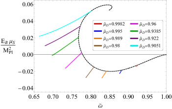
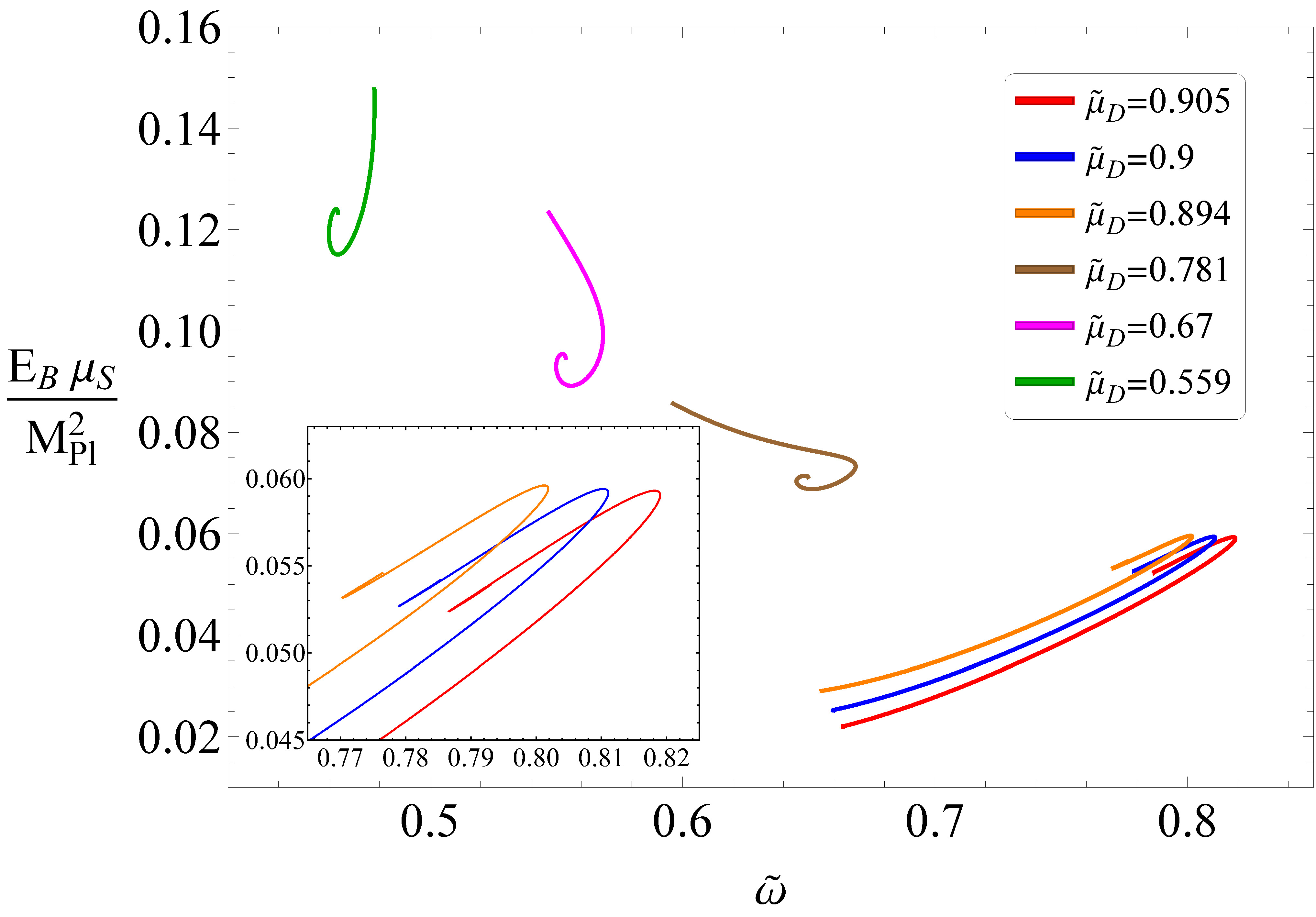
Figure 11: Left: The binding energy $E_{B}$ of the one-branch solution family as a function of the synchronized frequency $\tilde{\omega}$ for several values of the Dirac field mass $\tilde{\mu}_{D}$. Right: Same as left panel for the multi-branch solution family. The black dashed line represents the $S_{0}$ state solutions. All solutions have $\tilde{\mu}_{S}=1$.

Table 3: For one-branch (left panel) and multi-branch (right panel) solution families, the maximum value $E_{max}$ and the minimum value $E_{min}$ of the binding energy $E_{B}$ of the DBSs, the synchronized frequency $\tilde{\omega}$ corresponding to $E_{max}$ and $E_{min}$ ($\omega_{max}$ and $\omega_{min}$). $\omega_{0}$ is the value of the synchronized frequency $\tilde{\omega}$ when $E_{B}=0$.

$\tilde{\mu}_{D}$	$E_{max}$	$E_{min}$	$\omega_{max}$	$\omega_{min}$	$\omega_{0}$
$0.9982$	$-0.012$	$-0.014$	$0.923$	$0.921$
$0.98$	$-0.015$	$-0.027$	$0.808$	$0.787$
$0.96$	$0.003$	$-0.016$	$0.776$	$0.733$	$0.770$
$0.9385$	$0.021$	$-0.001$	$0.768$	$0.698$	$0.701$
$0.922$	$0.034$	$0.011$	$0.772$	$0.679$
$0.9051$	$0.052$	$0.022$	$0.801$	$0.664$

(a)

$\tilde{\mu}_{D}$	$E_{max}$	$E_{min}$	$\omega_{max}$	$\omega_{min}$	$\omega_{0}$
$0.905$	$0.059$	$0.022$	$0.818$	$0.664$
$0.9$	$0.059$	$0.025$	$0.810$	$0.659$
$0.894$	$0.060$	$0.030$	$0.801$	$0.655$
$0.781$	$0.086$	$0.069$	$0.596$	$0.651$
$0.67$	$0.124$	$0.089$	$0.547$	$0.556$
$0.559$	$0.148$	$0.115$	$0.478$	$0.464$

At the end of this section, we will analyse the binding energy $E_{B}=M-\mu_{S}Q_{S}-2\mu_{D}Q_{D}$ of the five solution families mentioned above. The binding energy $E_{B}$ of the DBSs versus the synchronized frequency $\tilde{\omega}$ for several values of the mass $\tilde{\mu}_{D}$ are presented in Fig. 11. In the left panel, fix the value of the Dirac field mass $\tilde{\mu}_{D}$, the binding energy $E_{B}$ of the DBSs increases with increasing synchronized frequency $\tilde{\omega}$. When the value of $\tilde{\mu}_{D}$ is sufficiently small, some unstable solutions ($E_{B}>0$) will occur. For the multi-branch solution family (right panel), the relationship between the binding energy $E_{B}$ of DBSs and the synchronized frequency $\tilde{\omega}$ is complicated, and there is no stable DBSs ($E_{B}>0$).

In Table 3, we show the maximum and minimum values of the binding energy $E_{B}$ of the DBSs in Fig. 11, the synchronized frequency $\tilde{\omega}$ corresponding to the maximum and minimum values of $E_{B}$, and the value of the synchronized frequency $\tilde{\omega}$ when $E_{B}=0$. For the one-branch solution family, both $E_{max}$ and $E_{min}$ increase as the Dirac field mass $\tilde{\mu}_{D}$ decreases, and there is no $\omega_{0}$ for the DBSs with higher or lower Dirac field mass $\tilde{\mu}_{D}$. For the multi-branch solution family, both $E_{max}$ and $E_{min}$ increase as the mass $\tilde{\mu}_{D}$ decreases, and there is no $\omega_{0}$ for the DBSs.

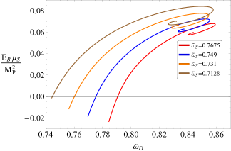
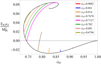
Figure 12: Left: The binding energy $E_{B}$ of the multi-branch solution family as a function of the nonsynchronized frequency $\tilde{\omega}_{D}$ for several values of the scalar field frequency $\tilde{\omega}_{S}$. Right: Same as left panel for the one-branch-A and one-branch-B solution families. The black dashed line represents the $D_{0}$ state solutions. All solutions have $\tilde{\mu}_{S}=\tilde{\mu}_{D}=1$.

Table 4: For multi-branch(left panel), one-branch-A(middle panel) and one-branch-B(right panel) solution families, the maximum value $E_{max}$ and the minimum value $E_{min}$ of the binding energy $E_{B}$ of the DBSs, the nonsynchronized frequency $\tilde{\omega}_{D}$ corresponding to $E_{max}$ and $E_{min}$($\omega_{Dmax}$ and $\omega_{Dmin}$). $\omega_{D0}$ is the value of the nonsynchronized frequency $\tilde{\omega}_{D}$ when $E_{B}=0$.

$\tilde{\omega}_{S}$	$E_{max}$	$E_{min}$	$\omega_{max}$	$\omega_{min}$	$\omega_{D0}$
$0.7675$	$0.068$	$-0.023$	$0.857$	$0.784$	$0.791$
$0.749$	$0.072$	$-0.018$	$0.852$	$0.770$	$0.775$
$0.731$	$0.078$	$-0.011$	$0.849$	$0.756$	$0.760$
$0.7128$	$0.084$	$-0.001$	$0.849$	$0.744$	$0.745$

(a)

$\tilde{\omega}_{S}$	$E_{max}$	$E_{min}$	$\omega_{max}$	$\omega_{min}$	$\omega_{D0}$
$0.9082$	$-0.015$	$-0.017$	$0.9105$	$0.9104$
$0.861$	$-0.020$	$-0.025$	$0.8667$	$0.8662$
$0.814$	$-0.016$	$-0.028$	$0.826$	$0.824$
$0.7676$	$0.019$	$-0.023$	$0.596$	$0.651$	$0.791$

$\tilde{\omega}_{S}$	$E_{max}$	$E_{min}$	$\omega_{max}$	$\omega_{min}$	$\omega_{D0}$
$0.7127$	$0.084$	$-0.001$	$0.849$	$0.744$	$0.745$
$0.702$	$0.083$	$0.007$	$0.821$	$0.738$
$0.691$	$0.078$	$0.018$	$0.794$	$0.734$
$0.6794$	$0.066$	$0.037$	$0.762$	$0.734$

The binding energy $E_{B}$ of the DBSs versus the nonsynchronized frequency $\tilde{\omega}_{D}$ for several values of the scalar field frequency $\tilde{\omega}_{S}$ are presented in Fig. 12. For the multi-branch solution family, with the increase of nonsynchronized frequency $\tilde{\omega}_{D}$, the binding energy $E_{B}$ of DBSs first increases, then turns to the second branch, and then changes in a spiral shape. For the one-branch-A solution family, the DBSs are stable ($E_{B}<0$) when the scalar field frequency $\tilde{\omega}_{S}$ is sufficiently large, and unstable DBSs ($E_{B}>0$) appear as the scalar field frequency $\tilde{\omega}_{S}$ decreases. For the one-branch-B solution family, stable DBSs hardly exist.

In Table 4, we show the maximum and minimum values of the binding energy $E_{B}$ of the DBSs in Fig. 12, the nonsynchronized frequency $\tilde{\omega}_{D}$ corresponding to the maximum and minimum values of $E_{B}$, and the value of the nonsynchronized frequency $\tilde{\omega}_{D}$ when $E_{B}=0$. For the multi-branch solution family, as the scalar field frequency $\tilde{\omega}_{S}$ decreases, both $E_{max}$ and $E_{min}$ increase and $\omega_{D0}$ decreases. For the one-branch-A solution family, as the scalar field frequency $\tilde{\omega}_{S}$ decreases, $E_{max}$ and $E_{min}$ first decrease and then increase, and $\omega_{D0}$ occurs. For the one-branch-B solution family, as the scalar field frequency $\tilde{\omega}_{S}$ decreases, $E_{max}$ decreases and $E_{min}$ increases, $\omega_{D0}$ disappears.

V Conclusions

In this paper, we construct spherically symmetric multistate Dirac-boson stars consisting of a scalar field and two spin fields, both in the ground state. Furthermore, the characteristics of different types of solution families of DBSs are discussed.

First, for the case of synchronized frequency, we divide the solution families of DBSs into one-branch and multi-branch based on the number of branches of the solutions. For the one-branch solution family, as the synchronized frequency $\tilde{\omega}$ increases, $\phi_{max}$ increases and $f_{max}$ and $g_{max}$ decrease. Moreover, the mass $M$ of DBSs decreases as $\tilde{\omega}$ decreases, while the binding energy $E_{B}$ changes in the opposite direction. In addition, the existence domain of the synchronous frequency $\tilde{\omega}$ increases as the mass $\tilde{\mu}_{D}$ of the Dirac field decreases. For the multi-branch solution family, the curve of the mass $M$ versus the synchronized frequency $\tilde{\omega}$ is spiral, and no similar family of solutions was found in Ref. Li:2019mlk . For the first branch of the DBSs, $\phi_{max}$ increases as the synchronized frequency $\tilde{\omega}$ increases, $f_{max}$ and $g_{max}$ first decrease and then increase. For the second and third branches of the DBSs, as the synchronized frequency $\tilde{\omega}$ increases, $\phi_{max}$, $f_{max}$ and $g_{max}$ all have monotonic behaviour. For each branch, the existence domain of the synchronized frequency $\tilde{\omega}$ increases as the mass $\tilde{\mu}_{D}$ of the Dirac fields decreases. Furthermore, as the mass $\tilde{\mu}_{D}$ decreases, $M_{min}$ increases, and $M_{max}$ first decreases and then increases. It is worth noting that for the family of multi-branch solutions, all solutions are unstable ($E_{B}>0$).

Then, for the case of nonsynchronized frequency, we divide the solution families of DBSs into multi-branch, one-branch-A and one-branch-B. For the multi-branch solution family, in contrast to the case of synchronized frequency, $\phi_{max}$, $f_{max}$ and $g_{max}$ have monotonic behaviour on all three branches as the nonsynchronized frequency $\tilde{\omega}_{D}$ increases. For each branch, the existence domain of the nonsynchronized frequency $\tilde{\omega}_{D}$ decreases as the frequency $\tilde{\mu}_{S}$ of the scalar field decreases. And as the frequency $\tilde{\mu}_{S}$ decreases, both $M_{min}$ and $M_{max}$ decrease. Furthermore, the stable solution ($E_{B}<0$) exists only on the first branch. For the one-branch-A solution family, as the nonsynchronized frequency $\tilde{\omega}_{D}$ increases, $\phi_{max}$, $f_{max}$, $g_{max}$, the mass $M$ and the existence domain of the nonsynchronized frequency $\tilde{\omega}_{D}$ vary in the same way as in the one-branch solution family for the case of synchronized frequency. However, for the case of nonsynchronized frequency, $M_{min}$ in the one-branch-A solution family is determined by the scalar field frequency $\tilde{\mu}_{S}$. Moreover, no matter what value of the scalar field frequency $\tilde{\mu}_{S}$ is taken, there is always a stable solution (provided that this solution belongs to the one-branch-A solution family). For the one-branch-B solution family, as the nonsynchronized frequency $\tilde{\omega}_{D}$ increases, $f_{max}$ and $g_{max}$ increases, $\phi_{max}$ increases and then decreases, and the mass $M$ of the DBSs decreases. The existence domain of the nonsynchronized frequency $\tilde{\omega}_{D}$ decreases as the scalar field frequency $\tilde{\mu}_{S}$ increases. In addition, there are almost no stable solutions in the one-branch-B solution family.

The multi-branch solution family for the cases of the synchronized/nonsynchronized frequencies and the one-branch-B solution family for the cases of the nonsynchronized frequency are unique, as similar families of solutions have not been found in past studies of multistate boson stars Li:2019mlk ; Li:2020ffy . Moreover, these newly discovered solution families are relatively unstable (most of them satisfy $E_{B}>0$). We will continue to study DBSs. The scalar and Dirac fields in this work are in the ground state, and later we will consider the case where the scalar and Dirac fields are in different energy levels, respectively. Furthermore, we believe that spherically symmetric multistate Dirac stars (SMSDSs) should exist where the matter fields are several Dirac fields. The construction of the model for SMSDSs is also part of our future work.

Appendix

In order to study the Dirac equation in curved spacetime, we need to introduce the vierbein $e_{a}^{\alpha}$, defined by

$$g_{\alpha\beta}e_{a}^{\alpha}e_{b}^{\beta}=\eta_{ab}\,,$$ (26)

where $g_{\alpha\beta}$ is the curved space metric and $\eta_{ab}=(-1,+1,+1,+1)$. We use Greek letters $\alpha,\beta,\cdots$ for curved spacetime indices and the Latin letters $a,b,\cdots$ for flat spacetime indices. Greek indices are raised and lowered with $g_{\alpha\beta}$ and Latin indices are raised and lowered with $\eta_{ab}$.

$\gamma^{a}$ are flat spacetime $\gamma$-matrices and $\gamma^{\alpha}$ are curved spacetime $\gamma$-matrices. $\gamma^{a}$ are related to $\gamma^{\alpha}$ through the vierbein:

$$\gamma^{\alpha}=e_{a}^{\alpha}\gamma^{a},\qquad\gamma^{a}=e^{a}_{\alpha}\gamma^{\alpha}.$$ (27)

$\gamma^{a}$ and $\gamma^{\alpha}$ satisfying the anticommutation relations:

$$\{\gamma^{\alpha},\gamma^{\beta}\}=2g^{\alpha\beta},\qquad\{\gamma^{a},\gamma^{b}\}=2\eta^{ab}.$$ (28)

$\gamma$-matrices indices are raised and lowered in the following ways:

$$\gamma_{a}=\eta_{ab}\gamma^{b},\qquad\gamma_{\alpha}=g_{\alpha\beta}\gamma^{\beta}.$$ (29)

The non-zero component of the vierbein we choose in this paper is

$$e_{0}^{t}=\frac{1}{\sqrt{N}\sigma},\quad e_{1}^{\theta}=\frac{1}{r},\quad e_{2}^{\varphi}=\frac{\csc\theta}{r},\quad e_{3}^{r}=\sqrt{N}.$$ (30)

For $\gamma^{a}$ we use the Weyl representation:

$$\gamma^{0}=i\begin{pmatrix}0&1\\ 1&0\end{pmatrix},\qquad\gamma^{k}=i\begin{pmatrix}0&\sigma_{k}\\ -\sigma_{k}&0\end{pmatrix},\qquad k=1,2,3,$$ (31)

where $\sigma_{k}$ are the Pauli matrices:

$$\sigma_{1}=\begin{pmatrix}0&1\\ 1&0\end{pmatrix},\qquad\sigma_{2}=\begin{pmatrix}0&-i\\ i&0\end{pmatrix},\qquad\sigma_{3}=\begin{pmatrix}1&0\\ 0&-1\end{pmatrix}.$$ (32)

It can be obtained from Eq. (27), Eq. (30) and Eq. (31) that $\gamma^{\alpha}$ in this paper are

$$\gamma^{t}=\frac{\gamma^{0}}{\sqrt{N}\sigma},\qquad\gamma^{r}=\sqrt{N}\gamma^{3},\qquad\gamma^{\theta}=\frac{\gamma^{1}}{r},\qquad\gamma^{\varphi}=\frac{\csc\theta\gamma^{2}}{r}.$$ (33)

The covariant derivatives of $\overline{\Psi}^{(k)}$ and $\Psi^{(k)}$ are

$$\hat{D}_{\mu}\Psi^{(k)}=\partial_{\mu}\Psi^{(k)}+\Gamma_{\mu}\Psi^{(k)},\quad\hat{D}_{\mu}\overline{\Psi}^{(k)}=\partial_{\mu}\overline{\Psi}^{(k)}-\Gamma_{\mu}\overline{\Psi}^{(k)},$$ (34)

where $\Gamma_{\mu}=\omega_{\alpha bc}\gamma^{b}\gamma^{c}/4$, with $\omega_{\alpha bc}$ is the spin connection:

$$\omega_{\mu ab}=e_{a\nu}e_{b}^{\lambda}\Gamma_{\mu\lambda}^{\nu}-e_{b}^{\lambda}\partial_{\mu}e_{a\lambda}\,,$$ (35)

where $\Gamma_{\mu\lambda}^{\nu}$ is the affine connection.

References

- (1) J. A. Wheeler, “Geons,” Phys. Rev. 97 (1955), 511-536
- (2) E. A. Power and J. A. Wheeler, “Thermal Geons,” Rev. Mod. Phys. 29 (1957), 480-495
- (3) D. J. Kaup, “Klein-Gordon Geon,” Phys. Rev. 172 (1968), 1331-1342
- (4) R. Ruffini and S. Bonazzola, “Systems of selfgravitating particles in general relativity and the concept of an equation of state,” Phys. Rev. 187 (1969), 1767-1783
- (5) V. Sahni and L. M. Wang, “A New cosmological model of quintessence and dark matter,” Phys. Rev. D 62 (2000), 103517 [arXiv:astro-ph/9910097 [astro-ph]].
- (6) T. Matos and L. A. Urena-Lopez, “Quintessence and scalar dark matter in the universe,” Class. Quant. Grav. 17 (2000), L75-L81 [arXiv:astro-ph/0004332 [astro-ph]].
- (7) W. Hu, R. Barkana and A. Gruzinov, “Cold and fuzzy dark matter,” Phys. Rev. Lett. 85 (2000), 1158-1161 [arXiv:astro-ph/0003365 [astro-ph]].
- (8) A. Suárez, V. H. Robles and T. Matos, “A Review on the Scalar Field/Bose-Einstein Condensate Dark Matter Model,” Astrophys. Space Sci. Proc. 38 (2014), 107-142 [arXiv:1302.0903 [astro-ph.CO]].
- (9) L. Hui, J. P. Ostriker, S. Tremaine and E. Witten, “Ultralight scalars as cosmological dark matter,” Phys. Rev. D 95 (2017) no.4, 043541 [arXiv:1610.08297 [astro-ph.CO]].
- (10) L. E. Padilla, J. A. Vázquez, T. Matos and G. Germán, “Scalar Field Dark Matter Spectator During Inflation: The Effect of Self-interaction,” JCAP 05 (2019), 056 [arXiv:1901.00947 [astro-ph.CO]].
- (11) V. Cardoso and P. Pani, “Testing the nature of dark compact objects: a status report,” Living Rev. Rel. 22 (2019) no.1, 4 [arXiv:1904.05363 [gr-qc]].
- (12) C. A. R. Herdeiro, A. M. Pombo, E. Radu, P. V. P. Cunha and N. Sanchis-Gual, “The imitation game: Proca stars that can mimic the Schwarzschild shadow,” JCAP 04 (2021), 051 [arXiv:2102.01703 [gr-qc]].
- (13) J. C. Bustillo, N. Sanchis-Gual, A. Torres-Forné, J. A. Font, A. Vajpeyi, R. Smith, C. Herdeiro, E. Radu and S. H. W. Leong, “GW190521 as a Merger of Proca Stars: A Potential New Vector Boson of eV,” Phys. Rev. Lett. 126 (2021) no.8, 081101 [arXiv:2009.05376 [gr-qc]].
- (14) M. Bezares, M. Bošković, S. Liebling, C. Palenzuela, P. Pani and E. Barausse, “Gravitational waves and kicks from the merger of unequal mass, highly compact boson stars,” Phys. Rev. D 105 (2022) no.6, 064067 [arXiv:2201.06113 [gr-qc]].
- (15) M. Colpi, S. L. Shapiro and I. Wasserman, “Boson Stars: Gravitational Equilibria of Selfinteracting Scalar Fields,” Phys. Rev. Lett. 57 (1986), 2485-2488
- (16) E. W. Mielke and R. Scherzer, “Geon Type Solutions of the Nonlinear Heisenberg-Klein-Gordon Equation,” Phys. Rev. D 24 (1981), 2111
- (17) F. Kling and A. Rajaraman, “Profiles of boson stars with self-interactions,” Phys. Rev. D 97 (2018) no.6, 063012 [arXiv:1712.06539 [hep-ph]].
- (18) C. A. R. Herdeiro and E. Radu, “Asymptotically flat, spherical, self-interacting scalar, Dirac and Proca stars,” Symmetry 12 (2020) no.12, 2032 [arXiv:2012.03595 [gr-qc]].
- (19) P. Jetzer and J. J. van der Bij, “CHARGED BOSON STARS,” Phys. Lett. B 227 (1989), 341-346
- (20) P. Jetzer, P. Liljenberg and B. S. Skagerstam, “Charged boson stars and vacuum instabilities,” Astropart. Phys. 1 (1993), 429-448 [arXiv:astro-ph/9305014 [astro-ph]].
- (21) B. Kleihaus, J. Kunz, C. Lammerzahl and M. List, “Charged Boson Stars and Black Holes,” Phys. Lett. B 675 (2009), 102-115 [arXiv:0902.4799 [gr-qc]].
- (22) S. Kumar, U. Kulshreshtha and D. Shankar Kulshreshtha, “Boson stars in a theory of complex scalar fields coupled to the U(1) gauge field and gravity,” Class. Quant. Grav. 31 (2014), 167001 [arXiv:1605.07210 [hep-th]].
- (23) R. Harrison, I. Moroz and K. P. Tod, “A numerical study of the Schrödinger–Newton equations,” Nonlinearity 16 (2002) no.1, 101-122
- (24) F. E. Schunck and E. W. Mielke, “Rotating boson star as an effective mass torus in general relativity,” Phys. Lett. A 249 (1998), 389-394
- (25) S. Yoshida and Y. Eriguchi, “Rotating boson stars in general relativity,” Phys. Rev. D 56 (1997), 762-771
- (26) B. Kleihaus, J. Kunz and M. List, “Rotating boson stars and Q-balls,” Phys. Rev. D 72 (2005), 064002 [arXiv:gr-qc/0505143 [gr-qc]].
- (27) B. Hartmann, B. Kleihaus, J. Kunz and M. List, “Rotating Boson Stars in 5 Dimensions,” Phys. Rev. D 82 (2010), 084022 [arXiv:1008.3137 [gr-qc]].
- (28) F. Kling, A. Rajaraman and F. L. Rivera, “New solutions for rotating boson stars,” Phys. Rev. D 103 (2021) no.7, 075020 [arXiv:2010.09880 [hep-th]].
- (29) C. Herdeiro and E. Radu, “Construction and physical properties of Kerr black holes with scalar hair,” Class. Quant. Grav. 32 (2015) no.14, 144001 [arXiv:1501.04319 [gr-qc]].
- (30) R. Brito, V. Cardoso, C. A. R. Herdeiro and E. Radu, “Proca stars: Gravitating Bose–Einstein condensates of massive spin 1 particles,” Phys. Lett. B 752 (2016), 291-295 [arXiv:1508.05395 [gr-qc]].
- (31) I. Salazar Landea and F. García, “Charged Proca Stars,” Phys. Rev. D 94 (2016) no.10, 104006 [arXiv:1608.00011 [hep-th]].
- (32) F. Finster, J. Smoller and S. T. Yau, “Particle - like solutions of the Einstein-Dirac equations,” Phys. Rev. D 59 (1999), 104020 [arXiv:gr-qc/9801079 [gr-qc]].
- (33) F. Finster, J. Smoller and S. T. Yau, “Particle - like solutions of the Einstein-Dirac-Maxwell equations,” Phys. Lett. A 259 (1999), 431-436 [arXiv:gr-qc/9802012 [gr-qc]].
- (34) C. S. Bohun and F. I. Cooperstock, “Dirac-Maxwell solitons,” Phys. Rev. A 60 (1999), 4291 [arXiv:physics/0001038 [physics]].
- (35) V. Dzhunushaliev and V. Folomeev, “Dirac stars supported by nonlinear spinor fields,” Phys. Rev. D 99 (2019) no.8, 084030 [arXiv:1811.07500 [gr-qc]].
- (36) C. Herdeiro, I. Perapechka, E. Radu and Y. Shnir, “Asymptotically flat spinning scalar, Dirac and Proca stars,” Phys. Lett. B 797 (2019), 134845 [arXiv:1906.05386 [gr-qc]].
- (37) E. Daka, N. N. Phan and B. Kain, “Perturbing the ground state of Dirac stars,” Phys. Rev. D 100 (2019) no.8, 084042 [arXiv:1910.09415 [gr-qc]].
- (38) J. L. Blázquez-Salcedo, C. Knoll and E. Radu, “Boson and Dirac stars in dimensions,” Phys. Lett. B 793 (2019), 161-168 [arXiv:1902.05851 [gr-qc]].
- (39) J. L. Blázquez-Salcedo and C. Knoll, “Constructing spherically symmetric Einstein–Dirac systems with multiple spinors: Ansatz, wormholes and other analytical solutions,” Eur. Phys. J. C 80 (2020) no.2, 174 [arXiv:1910.03565 [gr-qc]].
- (40) M. Minamitsuji, “Stealth spontaneous spinorization of relativistic stars,” Phys. Rev. D 102 (2020) no.4, 044048 [arXiv:2008.12758 [gr-qc]].
- (41) P. E. D. Leith, C. A. Hooley, K. Horne and D. G. Dritschel, “Nonlinear effects in the excited states of many-fermion Einstein-Dirac solitons,” Phys. Rev. D 104 (2021) no.4, 046024 [arXiv:2105.12672 [gr-qc]].
- (42) A. Bernal, J. Barranco, D. Alic and C. Palenzuela, “Multi-state Boson Stars,” Phys. Rev. D 81 (2010), 044031 [arXiv:0908.2435 [gr-qc]].
- (43) H. B. Li, S. Sun, T. T. Hu, Y. Song and Y. Q. Wang, “Rotating multistate boson stars,” Phys. Rev. D 101 (2020) no.4, 044017 [arXiv:1906.00420 [gr-qc]].
- (44) H. B. Li, Y. B. Zeng, Y. Song and Y. Q. Wang, “Self-interacting multistate boson stars,” JHEP 04 (2021), 042 [arXiv:2006.11281 [gr-qc]].
- (45) M. Alcubierre, J. Barranco, A. Bernal, J. C. Degollado, A. Diez-Tejedor, M. Megevand, D. Nunez and O. Sarbach, “-Boson stars,” Class. Quant. Grav. 35 (2018) no.19, 19LT01 [arXiv:1805.11488 [gr-qc]].
- (46) M. Alcubierre, J. Barranco, A. Bernal, J. C. Degollado, A. Diez-Tejedor, M. Megevand, D. Núñez and O. Sarbach, “Dynamical evolutions of -boson stars in spherical symmetry,” Class. Quant. Grav. 36 (2019) no.21, 215013 [arXiv:1906.08959 [gr-qc]].
- (47) D. Guerra, C. F. B. Macedo and P. Pani, “Axion boson stars,” JCAP 09 (2019) no.09, 061 [erratum: JCAP 06 (2020) no.06, E01] [arXiv:1909.05515 [gr-qc]].
- (48) J. F. M. Delgado, C. A. R. Herdeiro and E. Radu, “Rotating Axion Boson Stars,” JCAP 06 (2020), 037 [arXiv:2005.05982 [gr-qc]].
- (49) J. F. M. Delgado, C. A. R. Herdeiro and E. Radu, “Kerr black holes with synchronized axionic hair,” Phys. Rev. D 103 (2021) no.10, 104029 [arXiv:2012.03952 [gr-qc]].
- (50) S. R. Dolan and D. Dempsey, “Bound states of the Dirac equation on Kerr spacetime,” Class. Quant. Grav. 32 (2015) no.18, 184001 [arXiv:1504.03190 [gr-qc]].
- (51) C. A. R. Herdeiro, A. M. Pombo and E. Radu, “Asymptotically flat scalar, Dirac and Proca stars: discrete vs. continuous families of solutions,” Phys. Lett. B 773 (2017), 654-662 [arXiv:1708.05674 [gr-qc]].