The Rotation Period Distribution in the Young Open Cluster NGC 6709

Open clusters serve as a useful tool for calibrating models of the relationship between mass, rotation, and age for stars with an outer convection zone due to the homogeneity of the stars within the cluster. Cluster to cluster comparisons are essential to determine whether the universality of spin-down relations holds. NGC 6709 is chosen as a more distant representative Pleiades-age cluster for which no rotation periods of members have previously been obtained. This cluster is at a distance of over 1 kpc and has two red giant members. Isochrones place the age of the cluster at around 150 Myr, or approximately the same age as the Pleiades. Photometry is obtained over a multi-month observing season at the robotic observatory STELLA. After basic processing, PSF photometry was derived using Daophot II, and a suite of related software allowed us to create time series of relative magnitude changes for each star. Four time series analysis methods are then applied to these light curves to obtain rotation periods for members stars. We obtain for the first time rotation periods for 45 FGK cluster members of NGC 6709. We plot the Gaia EDR3 colors of the member stars against their rotation periods and find a slow-rotating sequence with increasing rotation periods towards redder stars and a smaller clump of rapid rotators that have not yet joined this sequence. NGC 6709 has rotation periods very similar to that of another Pleiades-age open cluster, NGC 2516.

1 Introduction

The rotation periods of cool stars, both in open clusters and in the field, have attracted considerable attention in recent years. Not only does the rotation period provide the basic observable that governs the activity properties of cool stars, but it can also be measured very precisely. Furthermore, the rotation period distributions evince patterns (e.g., Barnes, 2003) that inform us about internal processes in stars or even their ages (e.g., Skumanich, 1972; Barnes, 2007). Open clusters are particularly valuable as calibrating objects, or more generally because they offer us homogeneous sample of coeval stars of the same composition. This paper contributes to that effort by presenting a newly determined rotation period distribution for a hitherto unstudied young open cluster NGC 6709.

The Sun is not unique as a star, and so the physics of the solar-wind and angular momentum of the Sun in studies by those such as Parker (1958) and Weber & Davis (1967) can be applied to stars. A star after formation should spin down as angular momentum is lost from the interactions of the stellar winds with magnetic fields (e.g., Mestel, 1968). This tendency for older stars to spin slower takes the form of $v\sin i\propto t^{-1/2}$ for solar mass stars, or Skumanich’s relationship (Skumanich, 1972). This relationship has been generalized to one where the rotation period depends on both the mass (or equivalently color) and age of a star. If such a relationship actually exists, then it can be inverted to provide the age of a star from its measured rotation period and color, a procedure that is called gyrochronology (Barnes, 2003).

Early measurements of stellar rotation predating large-format CCDs used $v\sin i$ measurements from spectroscopy (e.g., Gaige, 1993). Modern observing techniques allow more precise and unambiguous measurements of the rotation period via photometric changes. Thus, the most efficient way of observing the rotation rates of stars is through changes in brightness in a time series of observations of an object. Kron (1947) initially observed periodic changes in light curves due to large, cool star spots. FGKM stars have an outer convection zone, and the suppression of convection from the magnetic field causes a cool spot to form, analogous to the sunspots. As these spots rotate across the line of sight, a dip in the stellar brightness may be observed (e.g., Strassmeier, 2009). Since starspots are thought to last at least the order of a few months, the stellar rotation can then be extracted from a time series of observations of a star’s brightness.

Open clusters provide a rich laboratory for observing stellar rotation. Cluster members can be considered largely homogeneous in chemical composition and age (e.g., De Silva et al., 2006), and so observing the rotation rates of the FGK stars (and M-dwarfs where possible) can provide information about the dependence of rotation periods on mass. Furthermore, the age of the open cluster can be determined by other independent methods such as isochrones (e.g., Sandage & Eggen, 1969) and measurements of the chromospheric flux (e.g., Mamajek & Hillenbrand, 2008). Open clusters can therefore serve to calibrate the age-mass-rotation relationship essential to gyrochronology. This method of using individual open clusters as snapshots of stellar rotation at a single age only holds if all clusters of a similar age and metallicity show similar distributions in rotation periods. Cluster to cluster comparisons that become essential to this theory.

One benchmark candidate for young open clusters around the age 125 Myr is the well-studied Pleiades at a distance of 133 pc (e.g., van Leeuwen et al., 1987; Hartman et al., 2010; Rebull et al., 2016),. This cluster, along with the Hyades (e.g., Radick et al., 1987; Delorme et al., 2011; Douglas et al., 2019), was used to derive the Skumanich’s relationship for the evolution of rotation for solar-type stars. Fritzewski et al. (2020) (hereafter F20) compare the rotation rates of members of four other Pleiades-age clusters and find that all measured ones behave similarly.

NGC 6709 was chosen as a significantly more distant representative of Pleiades-age clusters with no previous observations of rotation rates of member stars. Several membership studies are available the in literature relying on either spectroscopic or proper motion membership determination methods (Hakkila et al., 1983; Tadross, 2001; Dias et al., 2001; Kharchenko et al., 2004; Vande Putte et al., 2010; Kharchenko et al., 2013; Dias et al., 2014; Sampedro et al., 2017; Cantat-Gaudin et al., 2018). It has two red giant members (Lindoff, 1968; Sears & Sowell, 1997; Ahumada & Lapasset, 2007; Mermilliod et al., 2008), possible Be stars (Schild & Romanishin, 1976; Subramaniam & Sagar, 1999), and possible blue stragglers (Ahumada & Lapasset, 2007). One of the red giants is a spectroscopic binary (Mermilliod et al., 2007) and the other is a possible member of a quadruple star system (Smiljanic et al., 2018).

The above-1000 pc distance and consequent faintness of the cluster has led some disparity in adopted parameters due to the difficulty in observing the cluster, although with the advent of Gaia, these values have been more in agreement in recent publications. Values for the $E_{B-V}$ color excess range from 0.28–0.35 (Johnson et al., 1961; Becker, 1963; Burki, 1975; Mermilliod, 1981; Subramaniam & Sagar, 1999; Tadross, 2001; Lata et al., 2002; Ahumada & Lapasset, 2007; Piskunov et al., 2007; Kharchenko et al., 2013; Joshi et al., 2016; Sampedro et al., 2017). Distance estimates range from 930–1253 pc (Johnson et al., 1961; Hoag & Applequist, 1965; Lindoff, 1968; Burki, 1975; Mermilliod, 1981; Hakkila et al., 1983; Barkhatova et al., 1987; Lynga & Palous, 1987; Leisawitz, 1988; Subramaniam & Sagar, 1999; Dias et al., 2001; Tadross, 2001; Loktin & Beshenov, 2003; Kharchenko et al., 2005; Cantat-Gaudin et al., 2018).

Age estimates based on various methods of isochrone fitting in literature have ranged from 65 Myr to 320 Myr. Earlier studies of NGC 6709 tend to obtain ages of less than 80 Myr (Lindoff, 1968; Burki, 1975; Mermilliod, 1981; Barkhatova et al., 1989) or older than 200 Myr (Barbaro et al., 1969; Sagar & Subramaniam, 1999; Subramaniam & Sagar, 1999), possibly due to instrument limitations at the time and the distance to NGC 6709. More recent studies place the age around 100–190 Myr (Tadross, 2001; Lata et al., 2002; Chen et al., 2003; Kharchenko et al., 2005; Ahumada & Lapasset, 2007; Wu et al., 2009; Vande Putte et al., 2010; Smiljanic et al., 2018; Cantat-Gaudin et al., 2020; Bossini et al., 2019).

Radial velocity measurements have only been obtained for a few member stars, including the red giant members. Hence, there is some degree of uncertainty, and published values range from $-7$ to $-13$ km$\cdot$s^-1 (Lynga & Palous, 1987; Kharchenko et al., 2005; Vande Putte et al., 2010; Kharchenko et al., 2013; Conrad et al., 2017; Soubiran et al., 2018). Metallicity is not well-measured for this cluster, but spectroscopy from UVES members from Gaia-ESO data have the cluster near solar values (Magrini et al., 2021).

This work is part of the STELLA Open Cluster Survey (SOCS). The survey observes multiple open clusters over periods of several months to obtain rotation periods. The objective is to establish the similarities between open clusters of similar ages as well as track the evolution of rotation periods over time with clusters of different ages (e.g., Fügner et al., 2011; Barnes et al., 2015).

2 Methods

In outline, to derive rotation periods for stars in NGC 6709, we observe the field over several months, a comparatively long baseline that is permitted by our robotic observing, determine which stars in the field belong to the cluster, and obtain their corresponding colors from literature. We then construct light curves for each star from the collection of frames. We then perform time series analyses to obtain rotation periods and error estimates for each member star.

2.1 Data Aquisition and Reduction

Table 1: Observations and Exposure times

Exposure	Start Date	End Date	Number of
time			observations
$[$s$]$	yyyy-mm-dd	yyyy-mm-dd
24	2016-04-16	2016-09-05	228
120	2016-04-20	2016-08-04	167
300	2015-05-26	2015-11-07	82

The observations were obtained using the 1.2 m telescope STELLA-I at the Izaña Observatory in Tenerife, Spain from May 2015 until September 2016. This is part of the STELLA robotic observatory which also includes the 1.2 m spectroscopic telescope STELLA-II. The observatory operates robotically each night via in-house custom-built software (Granzer, 2004), provided conditions are suitable for observing targets determined by a program with user-defined priorities. For more information about STELLA operation, please see Strassmeier et al. (2004), Strassmeier et al. (2010), and Weber et al. (2016).

The CCD resolution for the wide-field imager WiFSIP V2.0 is $4066\times 4064$ pixels, or $22\arcmin\times 22\arcmin$. A single field was used to observe NGC 6709 due to its relatively small angular size. This field contains over two-thirds of the member stars when centered on the cluster. Observations were acquired in the Johnson $V$ band with exposure times of 24 s, 120 s, and 300 s to retain sensitivity to as wide a range of bright (bluer) and faint (redder) stars as was practicable.

Table 1 summarizes the dates and total number of successful observations available for each exposure time, after discarding any unusable frames due to bad seeing, poor weather conditions, lunar proximity, and tracking errors. Significant numbers of such frames are a typical consequence of robotic observations. With the 24 s exposures, visits to the target happened up to ten times per night, although typically usable frames on any successful night were in the range of three to seven. For the longer exposures of 120 s, this dropped to a maximum of seven times per night, with typical values below six. And for the longest exposure time, the range was up to four times per night for the target. The maximum time baseline of observations for each exposure group is under six months to observe multiple theoretical variability cycles. This dataset exceeds our minimum requirement of 50 usable frames for each exposure time and the minimum acceptable time baseline of 60 days to preserve our sensitivity to the longer rotation periods.

2.1.1 Membership

Table 2: Properties of open cluster NGC 6709

Parameter	Value	Reference
Right Ascension	RA = 282.836 deg	1
Declination	Dec = +10.334 deg	1
Proper Motion	$\mu_{\rm{RA}}$ = 1.41 mas/yr	1
	$\mu_{\rm{Dec}}$ = -3.53 mas/yr	1
Parallax	$\pi$ = 0.911 mas	1
Radial Velocity	$v_{\rm{rad}}$ = -10.2 km/s	2
Age	$T=150$ Myr	3

We adopt the membership study of Cantat-Gaudin et al. (2018) (hereafter CG18) to define member stars as all stars in the study with a membership probability of $50\%$ or greater. This study makes use of the recent high-precision Gaia observations and includes many dimmer members that previous studies were unable to observe likely due to instrument limitations (e.g., Hakkila et al., 1983; Kharchenko et al., 2013; Dias et al., 2014). According to CG18, the mean proper motion of NGC 6709 is $\mu_{\mathrm{RA}}=1.414$ mas yr^-1 and $\mu_{\mathrm{Dec}}=-3.532$ mas yr^-1, and the distance is 1064 pc. The properties we adopt for NGC 6709 and references are listed in Table 1. The study by CG18 with our membership criteria provides 299 open cluster members total.

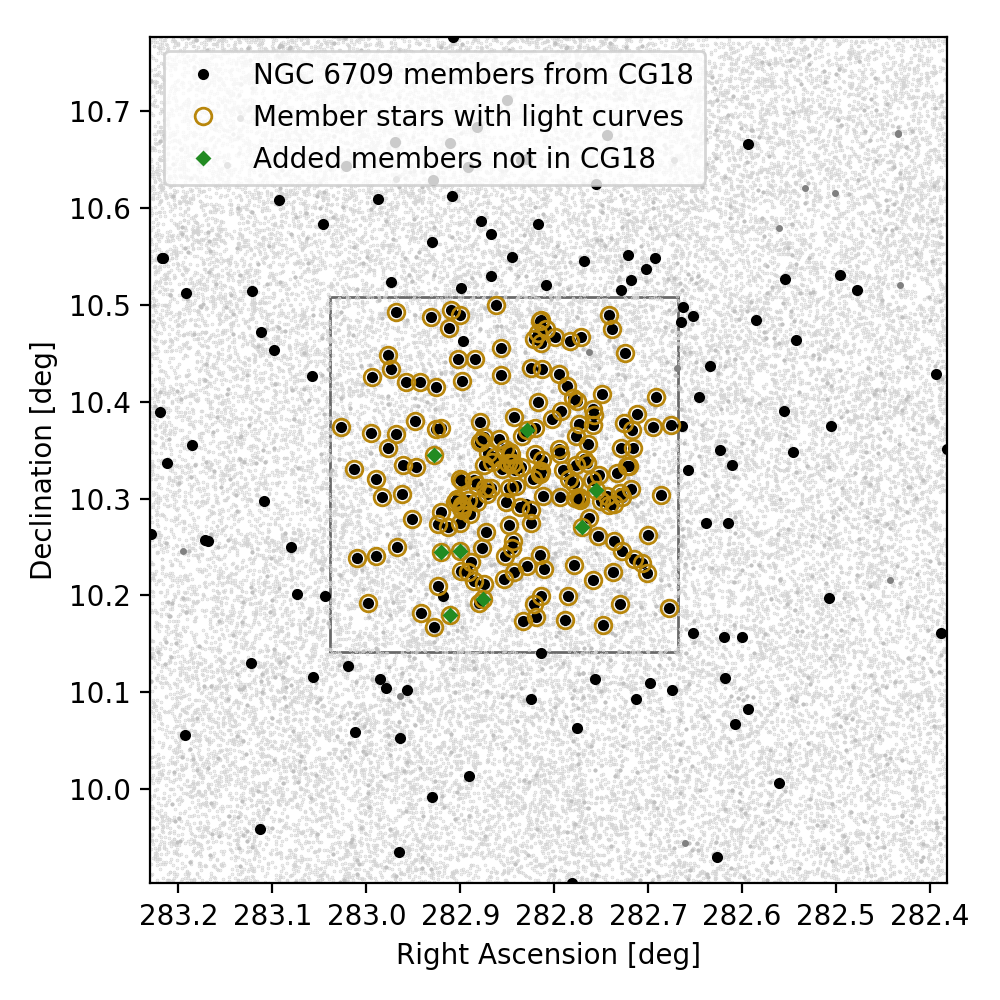
Figure 1: NGC 6709 members. The field of observation is centered on the dense center of the cluster and encompasses approximately two-thirds of the members. Stars used in this study are encircled, and our field of view is indicated by the square. Additional stars used as members in this study are shown as green diamonds.

Table 3: Additional cluster members

Designation	RA(1)	Dec(1)	$\mu_{\rm{RA}}$	$\mu_{\rm{Dec}}$	$\pi$	Prob(2)
Gaia EDR3	[deg]	[deg]	[mas/yr]	[mas/yr]	[mas]
4311548412384207488	282.911	10.180	$1.69\pm 0.08$	$-3.53\pm 0.08$	$0.87\pm 0.08$	0.7
4311549138251202560	282.875	10.196	$1.36\pm 0.19$	$-3.25\pm 0.18$	$0.85\pm 0.18$	0.5
4311549962915559168	282.900	10.246	$1.24\pm 0.09$	$-3.54\pm 0.10$	$0.95\pm 0.08$	0.7
4311549997275268352	282.921	10.245	$1.50\pm 0.08$	$-3.40\pm 0.07$	$0.83\pm 0.07$	0.8
4311553708127246848	282.771	10.270	$1.49\pm 0.15$	$-3.53\pm 0.16$	$0.94\pm 0.17$	0.8
4311559824161184128	282.928	10.345	$1.40\pm 0.15$	$-3.57\pm 0.17$	$0.89\pm 0.14$	0.8
4311600918410547712	282.755	10.309	$1.46\pm 0.03$	$-3.73\pm 0.03$	$0.89\pm 0.04$	0.6
4311607373703421056	282.829	10.371	$1.67\pm 0.03$	$-3.40\pm 0.03$	$1.04\pm 0.03$	0.6

Figure 1 shows the location of all stars with membership probability $\geq 0.5$ and the stars used in this study. Our field of observation covers the denser cluster center, and so we have observations for 210 of the cluster members. CG18 was limited to stars with $m_{G}<18$ due to the increase in errors at higher apparent magnitudes. This effectively limits the determination of membership for stars of NGC 6709 to K-stars or bluer due to the distance and reddening of the cluster. We search for possible additional members not included in CG18 using the Gaia EDR3 proper motion data and membership equation of Sagar (1987). These additional stars are listed in Table 2 and are the circled diamonds in Figure 1. Radial velocity measurements for cluster members are sparse, with measurements mainly obtained from the red giants and a few other bright members (e.g., Subramaniam & Sagar, 1999; Mermilliod et al., 2008; Kharchenko et al., 2013; Soubiran et al., 2018) and so membership through radial velocity measurements is not possible with existing surveys.

2.2 Catalogs

Supporting data for observations in standard passbands are taken from the literature by cross-referencing the coordinates of stars in our field with widely used catalogs. The coordinates were obtained by converting pixel coordinates to sky coordinates using WCSTools (Mink, 1997) and then matched to catalogs with Astropy (Astropy Collaboration et al., 2018). We use the UCAC4 catalog for measurements in the $B$ and $V$ passbands (Zacharias et al., 2013) and the Gaia EDR3 catalog for $G$, $G_{BP}$, and $G_{RP}$ s(Gaia Collaboration et al., 2016, 2020). We find some improvement in the Gaia colors with the EDR3 catalog over the DR2 values given in CG18.

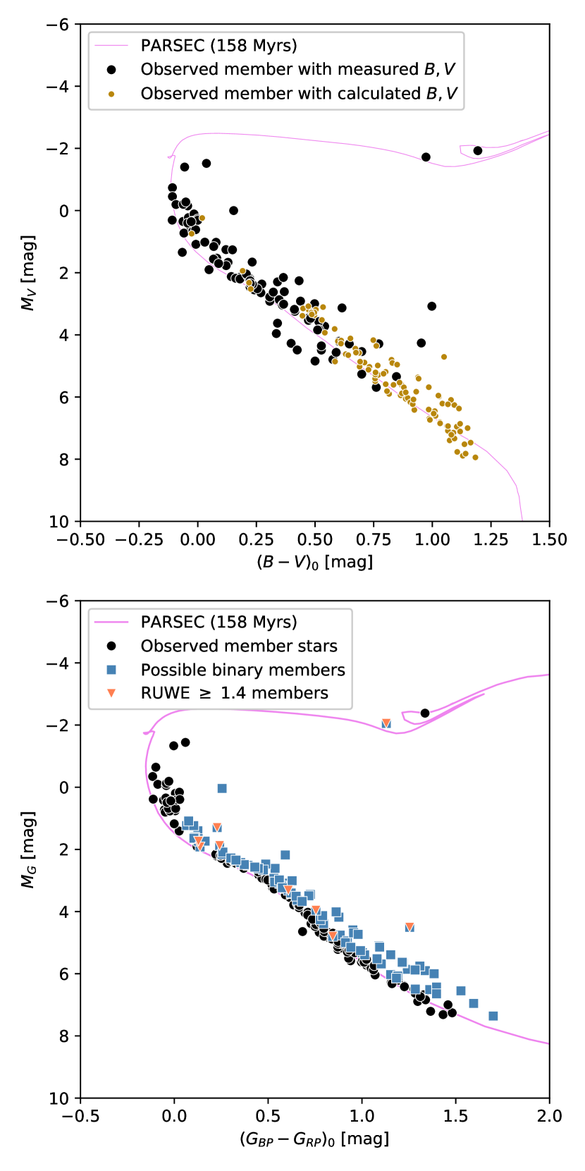
Figure 2: Color magnitude diagrams for NGC 6709 in $B-V$ (above), and Gaia color (below). PARSEC isochrones for $\log$Age = 8.2 are also displayed. The line-of-sight extinction is calculated for each star using individual stellar parallaxes as measured by Gaia instead of the mean cluster distance. Calculated $(B-V)_{0}$ from Gaia colors are shown in gold (above). Photometric binaries are indicated in blue and RUWE-value binaries are indicated in red (below).

We primarily utilize the Gaia EDR3 colors for this work as it is the most complete catalog to date with photometry for almost all of the stars in our field. Observations in the $B$ and $V$ passbands only exist for the brighter stars and hence are available for only a fraction of our cluster members. In order to facilitate a comparison with studies performed in $B-V$ colors, we use the equations in Appendix A of Gruner & Barnes (2020) to calculate values for $B-V$ from $G_{BP}-G_{RP}$ when no such values can be found in the UCAC4 catalog. The conversions between the two are piece-wise empirical functions fit to, among others, the Pleiades and so should be reasonable for NGC 6709.

2.2.1 Open Cluster Parameters of NGC 6709

Table 4: Adopted Parameters used for NGC 6709

Parameter	Value
Metallicity	Z = 0.013
Reddening	$E(G_{BP}-G_{RP})$ = 0.39 mag
	$E(B-V)$ = 0.29 mag
Extinction	$A_{G}$ = 0.78 mag
	$A_{V}$ = 0.90 mag

Values for reddening are selected based on literature values and adjusted by fitting isochrones. Literature values fall in the relative range from 0.28 (Kharchenko et al., 2013) to 0.35 (Subramaniam & Sagar, 1999) for $E(B-V)$. We use the relations from Gruner & Barnes (2020) of:

$$E(G_{BP}-G_{RP})=1.339\cdot E(B-V),$$ (1)

$$A_{G}=2.0\cdot E(G_{BP}-G_{RP}),$$ (2)

and

$$A_{V}=3.1\cdot E(B-V).$$ (3)

Gaia EDR3 measured parallaxes for each star are used for the distance modulus calculation, rather than a single value for the entire cluster.

We use a fit to solar-metallicity PARSEC isochrones for 158 Myr to determine a good reddening value for this work (Bressan et al., 2012). We select solar metallicity based on the spectroscopic analysis of Smiljanic et al. (2018) for the red giant member BD+10 3697 (Gaia EDR3 4311559274405377280), where [Fe/H] $=-0.01$. This isochrone also provides a good fit for the two red giants in the membership study of CG18. The CMDs corrected with the values in Table 4 are shown in Figure 2 for $(B-V)_{0}$ versus $M_{V}$ and $(G_{BP}-G_{RP})_{0}$ versus $M_{G}$. Where measurements are lacking for $M_{B}$ and $M_{V}$, we instead use the conversion of Gruner & Barnes (2020) to convert the Gaia colors to Johnson colors and fill in the lower right of the main sequence in the upper panel as well as a few brighter members which also lack observations in both $B$ and $V$. Also shown is the PARSEC isochrone. Binaries in the lower panel are either determined by their location above the main sequence or by the corresponding Gaia re-normalized unit weight error measurements where $RUWE<1.4$ indicates a good astrometric solution and hence single star, and values above this indicate a possible multistar system (Gaia Collaboration et al., 2016). We indicate which type of binary (photometric or RUWE) in Figure 2, bottom.

2.3 Construction of Light Curves

The light curves for individual stars are constructed using Daophot II (Stetson, 1987; Stetson et al., 1990). First, one master frame for each exposure time was selected from all the usable observations. We selected frames from the following dates: 2016-07-09 for 24 s, 2016-05-31 for 120 s, and 2015-07-17 for 300 s. These frames were selected based on low levels of light contamination, the goodness of the instrument focus, the lack of artifacts, and the low ellipticity of the stars. In order to use point-spread-function (PSF) photometry, suitable stars had to be selected from all possibilities found by Daophot II. Approximately 300 sources were selected for PSF photometry from the suggested PSF stars found by the program, and individually checked for counts comfortably between the background and saturation level and a minimum distance from other light sources of at least $15\arcsec$. Furthermore, a cross section examination of pixel values across these stars should have a single peak and the star circular. As a final step, any stars located near bad pixels were discarded.

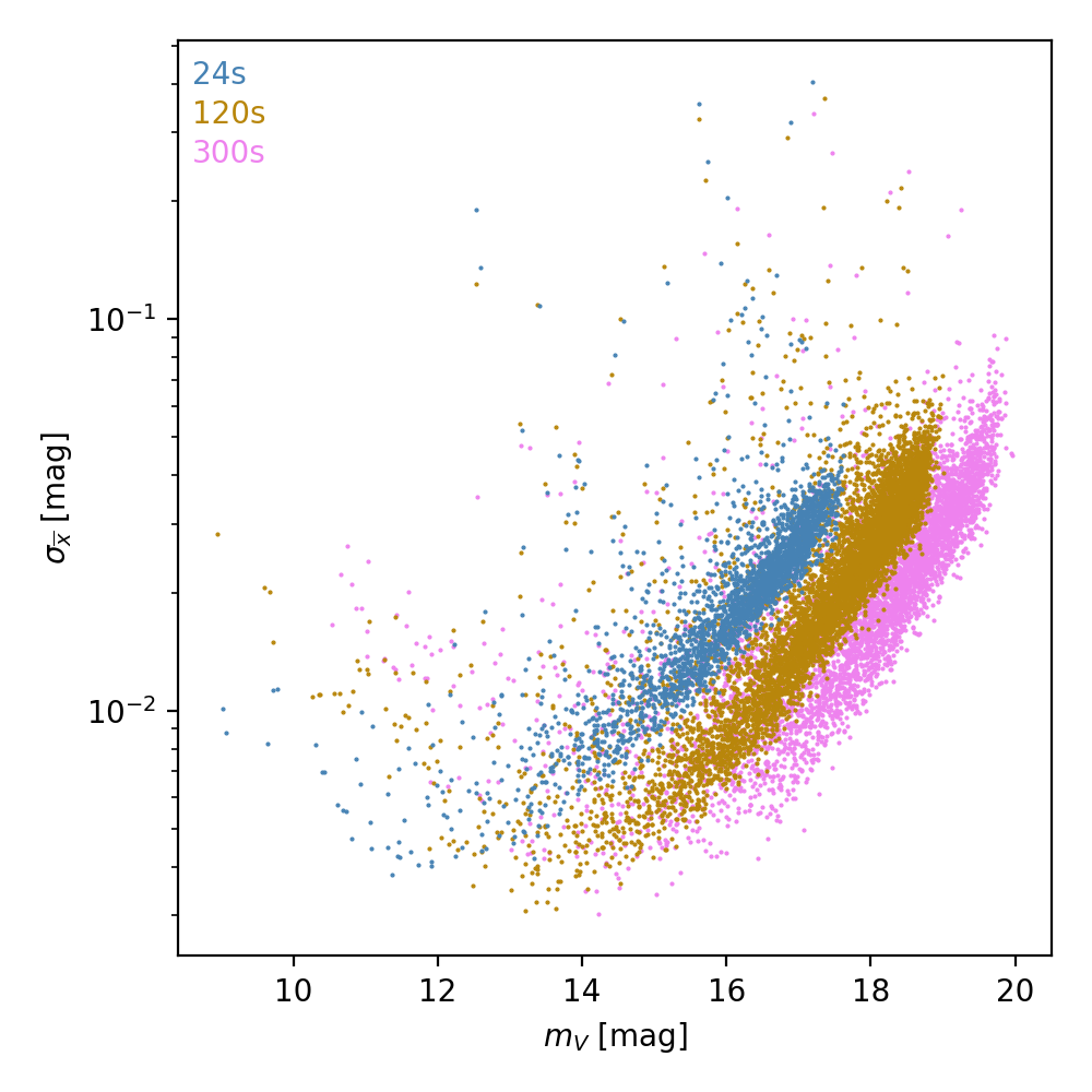
Figure 3: The mean magnitude versus standard error for all stars with light curves.

Once the stars for PSF photometry are selected, AllStar is used to find instrumental magnitudes for all sources in each frame using the stars assigned for the PSF photometry as a reference point. These magnitudes from each of these frames are then assembled as light curves using DaoMatch and DaoMaster. DaoMatch first pinpoints each source possible in every frame by taking the 30 brightest stars in each separate frame, matching triangles with the master frame, and deriving a coordinate transformation for use from frame to frame. DaoMaster then refines those transformations and applies them to all sources and assigns each source its own identifier across all frames. Each source is then outputted with its pixel location on the master frame and measured magnitudes from each frame, forming a time series for each star.

Figure 3 shows the mean apparent magnitude found by Daophot II versus the standard error $\sigma_{\overline{x}}$. Magnitude differences are detectable down to the millimag regime. The shift in the apparent magnitude access for each exposure set is the average of the difference between the $m_{V}$ determined by Daophot II and the apparent magnitude in the $V$-band for stars in the UCAC4 catalog. It can be seen that the fainter stars overall exhibit more uncertainty, and that the field contains some highly variable stars. The final step in producing the light curves was to remove outliers using the sigma clipping function in SciPy (Jones et al., 2001; Virtanen et al., 2020).

2.3.1 Time Series Analysis

To analyze the light curves, four methods were selected with the criteria of applicability to randomly spaced observations. The Phase Dispersion Minimization method (hereafter PDM) from Stellingwerf (1978) tests for periods that minimize the dispersion when the data are phased to the test periods. No a priori knowledge of the shape of the light curve is required for this method and so possible spot structure should not affect the results. The String Length method (hereafter SL) of Dworetsky (1983) phases the data with a test period and calculates a total “string length” between the data points, seeking periods that minimize this string length. Similar to the PDM, this method utilizes phase folding and seeks a minimum in the periodogram. This method is chosen as an alternative method to the PDM to examine the dispersion present in a phase-folded light curve.

The Generalized Lomb-Scargle method (or GLS) of Zechmeister & Kürster (2009) is a frequency analysis method that accounts for errors and offsets of the dataset. The GLS method can handle unevenly sampled data and fits the light curves to a combination of sine and cosine waves. We additionally use the CLEAN method of Roberts et al. (1987) which also samples frequencies but removes artifacts from unevenly sampled data such as the one-day alias. This serves as a complementary method to GLS in that it may amplify the true signal when more than one period is present in the data or there is a contribution of noise. Periods obtained via these methods appear as maxima in the periodograms.

2.3.2 Period Selection

After obtaining periodograms with the four methods, we select a period based on the following criteria:

1. There is agreement within 0.1 days between a primary dip in the PDM method and primary peak in the GLS method. There is similar evidence of minima/maxima in the periodograms of the SL and CLEAN methods.

2. The magnitude variations are higher than the noise from the constant stars of similar magnitudes.

3. The phase-folded data have a single maximum and minimum to avoid selecting a higher harmonic of the period.

4. The fit is valid across the most of the time series and there is a suitable density of observations.

Each criterion is given one point, and only periods that have three or four points total for at least one exposure time are selected as candidate periods for the stars.

The light curve and the selected period are visually inspected for each of the three exposure times independently. This system of determining periods tends to err on the side of caution in assigning a rotation period since each individual method does not always successfully recover the true rotation period and depends on factors such as the signal-to-noise ratio, object brightness, and sampling (e.g., Graham et al., 2013). 186 out of the 204 cluster member stars were found in more than one exposure batch, and so the selected periods at different exposure times for the same star are compared. In most cases, the discrepancy is less than 0.1 day, and the few exceptions are harmonics or subharmonics.

From the cases where a star has more than one possible period due to the multiple exposure times, we select as our period whichever fulfills more criteria, has the clearest peaks or dips in the periodograms, and has the most observations, in that order. In some cases, a period is not recovered at a different exposure time either because the exposure time was too short to capture the magnitude changes and variability, or the exposure time was too long and reached saturation.

2.3.3 Uncertainties in the Period

Error bars for periods are obtained from Gaussian fits to the corresponding period minimum in the PDM. Fits are made for PDMs with minima of 0.6, although exceptions are made for for those with a minimum between 0.6 and 0.8 that show a strong single peak in the GLS periodogram. We use the standard deviation $\sigma$ of the Gaussian distribution as an indication of the uncertainties in the periods so that wide peaks correspond to a larger uncertainty than narrow peaks. We use the only the error associated with the exposure the final period was selected from. Because this is selected via Gaussian distributions fit to the PDM periodogram, this $\sigma$ is accordingly only associated with the PDM method. The SL method does not provide clear minima in most cases, and the GLS and CLEAN methods use a grid in frequency space and thus skew the errors when translated to the period space.

3 Results

Table 5: Results for NGC 6709 Member Stars with $P_{\mathrm{rot}}$

Designation	RA(1)	Dec(1)	$(G_{BP}-G_{RP})_{0}$	$(B-V)_{0}$	$(B-V)_{\mathrm{calc}}\,^{(2)}$	Prob${}_{\mathrm{CG18}}\,^{(3)}$	$P_{\mathrm{rot}}$	$\sigma$
Gaia EDR3	[deg]	[deg]	[mag]	[mag]	[mag]		[d]	[d]
4311605728774145024	282.692	+10.405	0.872		0.692	1.0	5.59	0.22
4311599166063884288*	282.701	+10.263	1.361		1.134	0.8	7.42	0.37
4311552127579306624	282.706	+10.234	0.891	0.953		0.9	5.46	0.21
4311602017922290176	282.716	+10.352	0.772	0.576		0.6	4.22	0.08
4311552161939033984	282.728	+10.246	0.819	0.602		1.0	4.69	0.19
4311601983562535936	282.729	+10.353	0.798		0.626	1.0	4.36	0.18
4311551371664962048	282.730	+10.191	1.276		1.061	0.9	5.54	0.34
4311600780971586048	282.741	+10.294	0.871		0.692	1.0	5.63	0.17
4311600746611842816	282.751	+10.298	0.745		0.579	0.9	2.82	0.11
4311601120223606400*	282.752	+10.324	1.242		1.030	1.0	3.81	0.05
4311552230658504064	282.753	+10.261	1.062		0.866	0.9	2.26	0.02
4311602567678117248	282.759	+10.393	1.070		0.874	0.9	7.86	0.31
4311601536885870976	282.765	+10.337	0.696		0.538	1.0	0.71	0.10
4311611879167920896	282.771	+10.466	0.886		0.705	0.9	5.74	0.26
4311553914285720448*	282.774	+10.301	0.595		0.452	0.9	2.88	0.06
4311608477553696768	282.775	+10.401	1.015		0.823	0.9	9.01	0.22
4311601330727819648	282.776	+10.334	0.872		0.692	1.0	5.66	0.18
4311601743044328704	282.777	+10.365	0.840		0.663	1.0	1.01	0.10
4311553914285717632	282.778	+10.301	0.821		0.646	1.0	4.46	0.12
4311601262008339968	282.785	+10.321	0.800		0.628	0.9	4.63	0.11
4311550993707780224	282.786	+10.199	0.845	0.699		0.8	4.78	0.13
4311608511913447680*	282.786	+10.416	0.922		0.738	0.6	12.46	0.92
4311609233467993216	282.814	+10.461	1.034		0.841	0.9	6.97	0.33
4311607687279658496	282.817	+10.400	0.873		0.693	0.9	5.64	0.17
4311609267827745792	282.817	+10.470	0.750	0.500		0.9	2.65	0.04
4311552436816786304	282.829	+10.230	0.961		0.774	0.9	4.50	0.16
4311547798252006272	282.834	+10.174	0.447	0.307		0.9	1.79	0.02
4311607309322456704*	282.835	+10.365	0.912		0.729	0.9	5.60	0.15
4311554189163566720	282.840	+10.313	0.923		0.738	0.9	5.30	0.17
4311552780414370944	282.845	+10.249	0.756	0.772		0.9	2.86	0.09
4311560305197607296*	282.863	+10.343	1.090		0.892	0.9	2.28	0.02
4311553398889528320*	282.872	+10.305	1.002		0.811	1.0	6.12	0.10
4311608301417284736	282.885	+10.444	0.932	0.761		1.0	5.97	0.25
4311553330139990784	282.892	+10.298	1.049		0.854	0.7	6.95	0.29
4311607996517234048	282.898	+10.421	1.061		0.866	0.9	6.97	0.27
4311549859836309248	282.899	+10.225	1.156		0.952	1.0	3.09	0.05
4311553124011562368*	282.899	+10.290	1.308		1.089	0.6	7.36	0.21
4311610745296412800*	282.901	+10.489	1.153		0.950	1.0	7.95	0.42
4311559343130336128*	282.911	+10.324	0.925		0.740	0.8	5.17	0.14
4311548412384207488*	282.911	+10.180	1.184		1.030	(0.7)	3.22	0.08
4311609920662656512*	282.912	+10.476	0.429	0.322		0.7	2.81	0.06
4311553055261728256	282.913	+10.271	1.366		1.138	0.5	5.9	0.20
4311549997275268352*	282.921	+10.245	1.219		1.029	(0.8)	6.92	0.18
4311561095471630848*	282.925	+10.415	1.153		0.950	0.8	2.53	0.05
4311562435501392000	282.973	+10.433	1.011	0.699		1.0	6.56	0.28

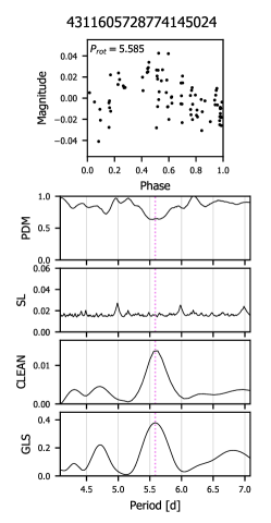
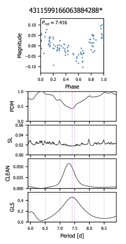
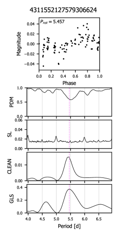
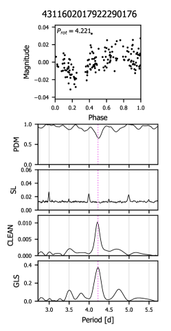
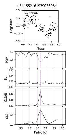
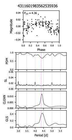
Figure 7: Phased light curves and results of period analysis methods. An asterisk after the Gaia designation and blue phased light curve indicates a possible binary. The vertical dotted line marks the found period.

Each exposure time group was analyzed independently in Daophot II. This allowed for confirmation of rotation periods among stars that appeared in more than one exposure group. Of the 210 cluster members mentioned in Section 2.1.1, we constructed lightcurves for 187 probable members. Of these, 182 are FGK stars and 5 are A stars. From these, we find periods for 45 FGK cluster members and 2 of the A stars. All rotation periods found and the Gaia EDR3 designations along with catalog and calculated colors are shown in Table 3. Final periods were selected via the method outlined in 2.3.2. Stars either showed agreement between different exposure times within a few percent, or the harmonic or subharmonic periods produced a stronger signal at a different exposure. The phased light curves and results from the period analysis methods for all member stars are shown in the Appendix Figure 7. All possible binary stars with strong period signals are photometric, with RUWE values between 0.86 and 1.13. In most cases, the selected period shows agreement between the PDM, Clean, and GLS methods, but in a few cases the noise level is higher than the magnitude changes and the minima with the PDM methods are weak, and so we pick our periods from the CLEAN and GLS methods. The SL method is primarily useful for confirming a period in the PDM of less than three days. With each phased light curve, we subtract the mean.

3.1 The Color-Period Diagram

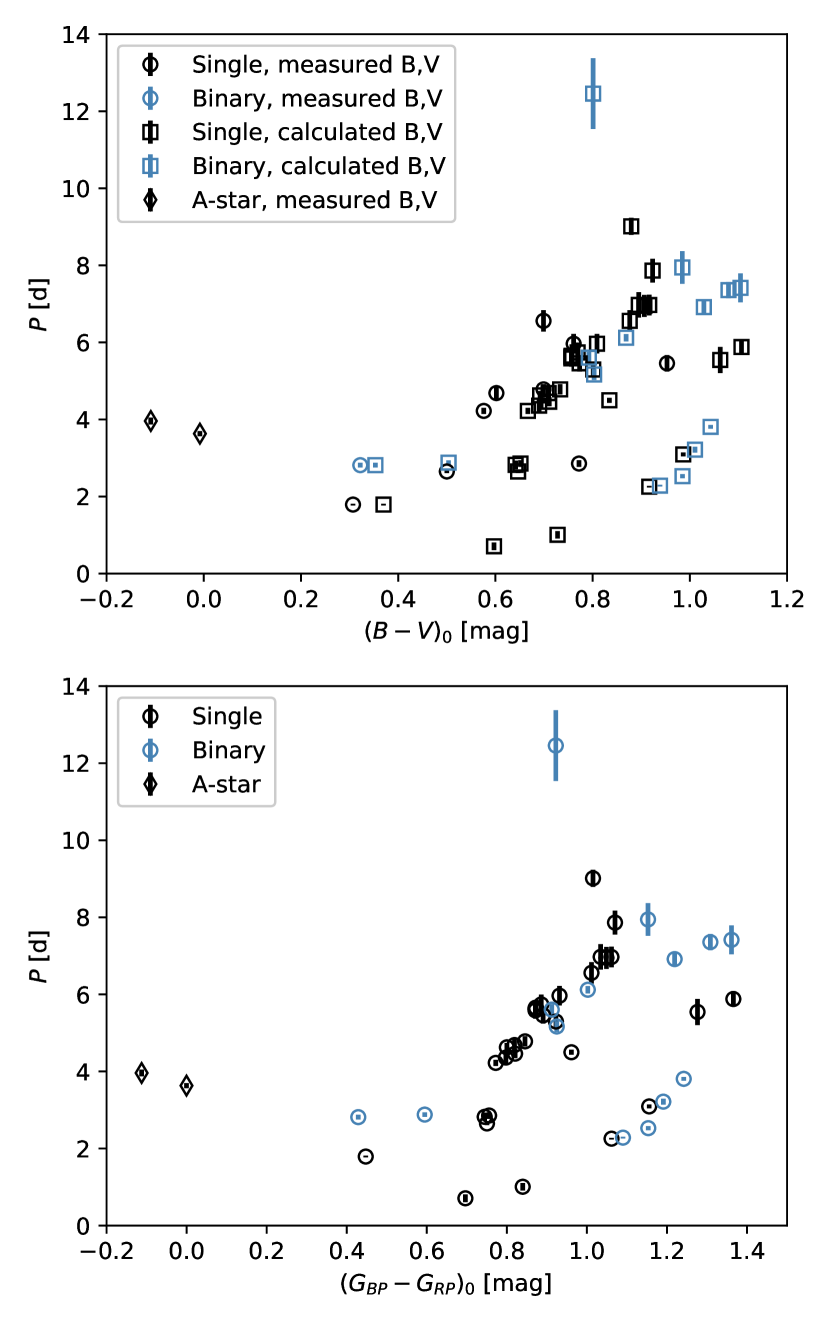
Figure 4: Rotation periods versus $(B-V)_{0}$ (top) and $(G_{BP}-G_{RP})_{0}$ (bottom). Error bars are the $\sigma$-value of the Gaussian fit to the minimum at the period in the PDM periodogram. Squares in $(B-V)_{0}$ indicate magnitudes calculated from $(G_{BP}-G_{RP})_{0}$ while circles are magnitudes found in the UCAC4 and Gaia EDR3 catalogs (top and bottom respectively). Possible binaries are indicated in blue.

Our color-period diagram (hereafter CPD) is shown in Figure 4 for both $(B-V)_{0}$ and $(G_{BP}-G_{RP})_{0}$. We show the $(B-V)_{0}$ for comparison with other literature studies of rotation rates versus colors, but as can be seen here, the sequence demonstrates more spread than for $(G_{BP}-G_{RP})_{0}$ because the uncertainties in these colors are greater. The CPD shows a sequence of increasing rotation periods towards redder stars. Below this sequence there is a small clump of rapidly rotating K-stars, which is to be expected for a cluster that is younger than $\approx 200$ Myr. The photometric binaries lie below the slow rotator sequence, although these also have longer periods towards the cooler stars. NGC 6709, due to observational limits, lacks observations for the M-dwarfs. Above the slow rotator sequence, there is at least one probable binary with a much slower rotation period and a membership probability of $0.6$. There are also two bright A-type stars that had periodic brightening and dimming, but whether these are the result of being multi-star systems or some other phenomenon occurring in the line of sight is unknown. The rotation periods for these two stars only appeared in the 24 s exposure due to saturation at longer exposure times, but the periodic magnitude change is significant enough that a signal was found in multiple time series analysis methods.

4 Discussion

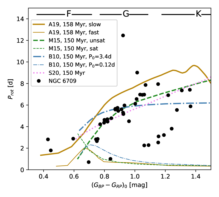
Figure 5: Rotation periods versus $(G_{BP}-G_{RP})_{0}$ for cluster members and comparison to models. A19 refers to the model by Amard et al. (2019), where both the sequences for initially slow and fast rotators are shown by solid and dashed lines, respectively. M15 is the model of Matt et al. (2015) with the unsaturated and saturated regimes indicated by solid and dotted lines, respectively. B10 is the model of Barnes & Kim (2010), with the solid and dashed lines again denoting initially slow and fast rotators. S20 is the model of Spada & Lanzafame (2020).

Due to the faintness of NGC 6709, we use the color system $G_{BP}$ and $G_{RP}$ from the Gaia EDR3 survey to avoid the necessity of converting the colors for the fainter stars that lack observations in other passbands. We use the conversion from Gruner & Barnes (2020) to convert between Gaia colors and Johnson colors. The two bluest stars with rotation periods from NGC 6709 are omitted from the discussion as these are A-type stars and lack a convection zone, considered a critical component for the dynamo type that supports the formation of star spots (e.g., Berdyugina, 2005). Thus, their periodicity is likely the result of being members of a multi-star system and actual rotation rate is unknown. For a more in-depth discussion of the behavior of these models including M-dwarfs, which are not present in our sample, please see F20.

4.1 Stellar spin-down models

We compare the results with several models of stellar rotation and age. These models are semi-empirical and use a theoretical framework built on the mechanisms thought to be responsible for stellar spin-down and are calibrated to observations of, for example, the Sun, or well studied clusters such as the Hyades. We select the models of Barnes & Kim (2010) (hereafter B10), Matt et al. (2015) (hereafter M15), Amard et al. (2019) (hereafter A19), and Spada & Lanzafame (2020) (hereafter S20) to derive theoretical isochrones for the estimated age of NGC 6709.

The isochrones from the models are plotted against the rotation periods found for NGC 6709 in Figure 5. All four stellar spin-down models have the same basic premise: a ZAMS star with some initial rotation rate $P_{0}$ will begin to spin down due to coupling of the magnetic field with the stellar wind. The spindown rate depends on the Rossby number

$$Ro=P_{\mathrm{rot}}/\tau_{\mathrm{conv}},$$ (4)

where $\tau_{\mathrm{conv}}$ is the convective turnover time. The selected models differ in some of the physical constraints and free parameters, but all reproduce to some degree the observed rotational behavior.

4.1.1 The Barnes & Kim 2010 model

The B10 model is a dimensionless description of period evolution over time. The equation combines the evolution of both the fast (C) and slow (I) sequences so that the period evolution equation is

$$t=\frac{\tau_{\mathrm{conv}}}{k_{C}}\ln\left(\frac{P_{\mathrm{rot}}}{P_{0}}\right)+\frac{k_{I}}{2\tau_{\mathrm{conv}}}\left(P_{\mathrm{rot}}^{2}-P_{0}^{2}\right).$$ (5)

where $t$ is the stellar age, $k_{C}$ and $k_{I}$ are dimensionless constants derived from observations, $P_{\mathrm{rot}}$ is the rotation period at stellar age, and $P_{0}$ is the initial rotation period. In order to be consistent with previous work, $\tau_{\mathrm{conv}}$ is the global $\tau_{c}$ from Table 1 of Barnes & Kim (2010), and the constants $k_{C}$ and $k_{I}$ are $0.646$ d Myr^-1 and $452$ Myr d^-1, respectively. The initial rotation of the fast sequence is $P_{0}=0.12$ d and for the slow sequence, $P_{0}=3.4$ d. These are based on observations of the extrema of initial rotation periods of young cluster members. The C and I sequences that emerge from these equations provide limiting cases.

The B10 model is shown in Figure 5 for an age of 150 Myr with initial rotation periods of 3.4 d and 0.12 d as the solid and dotted blue lines respectively to recreate the limits of the I and C sequences. This model results in rotation periods too slow for F-type stars and too fast for the K-type stars when compared to the observed rotation periods of NGC 6709 for the I sequence. There are no cluster members with rotation periods shorter than the limit created by the C sequence, which corresponds to stars with an initial rotation period of 0.12 d, which is near the break-up speed for FGK stars. The rapid rotators are not well-populated, at least partially due to the lack of observations for M-stars. Barnes et al. (2016) notes that this model does not account for evolution of the star pre-main sequence and works better for clusters and stars between 400 Myr and 2.5 Gyr. The model appears to have too aggressive of a spin down for young stars that are solar or hotter, and is not aggressive enough for young stars that are cooler. The G-type stars fit the model moderately well, which is not a surprise as the constants for this model were calibrated using the solar age and rotation period.

4.1.2 The Matt et al. 2015 model

The M15 model examines the changes in the torque over time on a star and the relationship with $Ro$. Stellar activity is divided into two regimes, saturated and unsaturated, based on whether magnetic activity indicators have approached some saturated values independent of $Ro$. The saturated and unsaturated regimes correspond to rapid and slow rotators, respectively. We model the limit of the saturated and unsaturated regimes, Equations 10 and 11 respectively in M15, and input an age of 150 Myr. The moment of inertia is from the stellar tracks of Baraffe et al. (2015) and the convective turnover time is based on the empirical relation given in Cranmer & Saar (2011), as the model is calibrated to these values for $\tau$. For the saturated limit, we use an initial rotation period of $P_{0}=0.2$ d. Using the adopted parameters provided in Table 1 in the Erratum which are adjusted to recreate solar values at a solar age, we show the model in Figure 5 with the solid line indicating the limit from the unsaturated regime and the dotted line the limit from the saturated regime.

The model provides a pretty good description of the G-stars and our few K-stars along the slow branch. Our F-stars show rotation periods where the model predicts either very rapid rotation or none at all. The saturated limit for the torque is similar to the lower limit of the most rapid rotators from the B10 model, although it allows for slightly more rapid rotation in the solar regime. Few cluster members actually lie near this limit, but instead occupy the space between.

4.1.3 The Amard et al. 2019 model

The rotation periods of A19 are based on models calculated using the STAREVOL v3.40 code. The models follow structural and rotational evolution and include the disc-coupling timescale and wind braking. To match our cluster, we use the models for solar metallicity ($Z=0.0134$) and an age of $\log T=8.2$, or 158 Myr. We show the models for both the slow and rapid rotators in Figure 5 as solid and dotted gold lines respectively. This corresponds to initial rotation rates of 1.6 days (2.3 days for stars with $M>1.2M\odot$) for the rapid rotators and 9.0 days for the slow rotators.

From the figure it can be seen that this model does not fit well, and a younger isochrone for the cluster would likely fit better as this one has an all-around too aggressive spin down for stars as compared to the other models. This model, however, does reproduce better the rotation rates of our few F-type stars. The lower limit for the rapid rotators matches fairly closely with the corresponding saturated limit of the M15 model for the G- and K-type stars. This is not entirely surprising as the torque at the surface uses the M15 formulation for the change in angular momentum.

4.1.4 The Spada & Lanzafame 2020 model

We also show the model of S20 in Figure 5 in violet. Unlike the previous models, this model has only the slow rotator sequence. The model scales rotational coupling and stellar wind braking with mass to explain the lack of low-mass stars that have reached the slow rotator sequence for clusters younger than 1 Gyr. We use the isochrones from Table A1 in the work of S10 for 150 Myr and the relation from Gruner & Barnes (2020) to convert $(B-V)_{0}$ to $(G_{BP}-G_{RP})_{0}$.

This model does reproduce fairly well the rotation periods for the K-type stars and the hotter G-type stars, but the spindown is not aggressive enough for the solar-type and cooler stars and the resulting rotation periods are too rapid compared to what has been observed for our cluster members.

4.2 Comparison to other open clusters

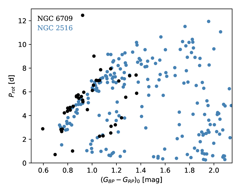
Figure 6: Overlay of the CPD of NGC 6709 on that of NGC 2516 from F20. The two distributions appear to be identical in the region of overlap.

We compare the CPD of NGC 6709 to the similarly aged clusters detailed in F20. It can be seen in Figure 6 from overlaying NGC 6709 with NGC 2516, the benchmark cluster from that work, that although NGC 6709 is fainter and has a few giant members, it exhibits almost identical rotational behavior. F20 also compare their open cluster with other similarly aged open clusters M35, the Pleiades, M50, and Blanco I in their Figure 17, and note the near identical structure of the rotation periods versus color. Our cluster is no exception, and fits in well with the age group of Pleiades-like open clusters.

The slow rotator sequence of NGC 6709 is very similar to that of NGC 2516. The slow-sequence for NGC 6709 is very slightly above that of NGC 2516, and so this cluster should accordingly be slightly older. There is an outlier with a much longer rotation period than expected ($\approx 12.5$ d), but similar outliers are observed for M35, the Pleiades, and M50. NGC 6709 also exhibits the gap between stars on the rapid rotator sequence and stars that have evolved onto the slow rotator sequence. The rapid rotators for NGC 6709 all have color values $(G_{BP}-G_{RP})_{0}<1.5$, and so a comparison of the structure of the rapid rotators that have not yet joined the slow rotator sequence is not possible.

5 Conclusions

We observe the open cluster NGC 6709 over multiple observing seasons to obtain for the first time 2–4 month long photometric light curves using Daophot II. Member FGK stars are identified and analyzed using four different methods (PDM, SL, GLS, and CLEAN) to find periodicities. By comparing the results from these four methods, we obtain rotation periods for 47 member stars within our field. We calculate the uncertainty of these rotation periods from the FWHM of the peak from the PDM method.

Using Gaia colors, we construct a color-period diagram of cluster members. This CPD has a sequence of slow rotators with increasing rotation periods towards the redder stars and a small clump of rapidly rotating stars that have not yet converged onto the aforementioned slow sequence. The six photometric binary members show no significant difference and follow the same pattern as other member stars. We compare isochrones from theoretical, empirical, and semi-empirical models for stellar rotation and evolution to our CPD and estimate the cluster age to be about 150 Myr. This is within the range of ages estimated from literature based on isochrones from color-magnitude comparisons. The models that best fit the CPD of NGC 6709 are those of M15 and S20.

The rotation periods follow a similar behavior as that observed in other open clusters of similar ages and characteristics. We compare this cluster’s CPD to NGC 2516 in the work of F20 and find that the rotation period distribution for NGC 6709 matches that of NGC 2516. F20 also compares NGC 2516 to four more open clusters of similar ages, the Pleiades, M35, M50, and Blanco I. This is further support that the mechanisms driving the star formation and subsequent spin-down for stars with similar parameters are the same for open clusters with sufficiently similar parameters of age and metallicity.

Appendix A Phased light curves for FGK member stars with rotation periods

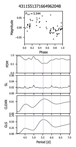
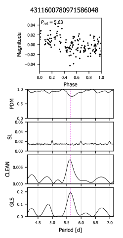
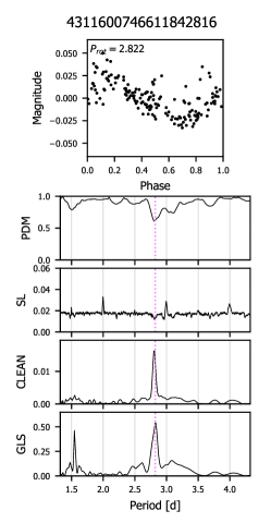
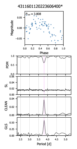
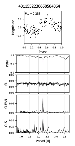
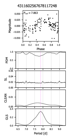
Figure 8: continued.

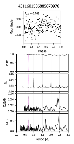
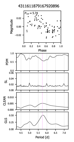
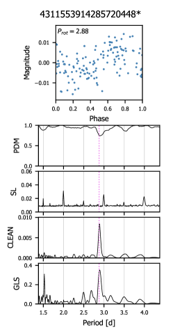
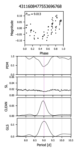
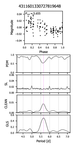
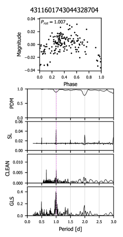
Figure 9: continued.

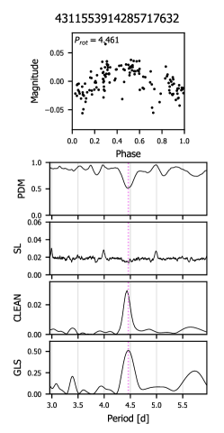
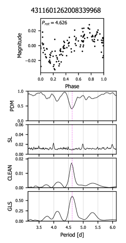
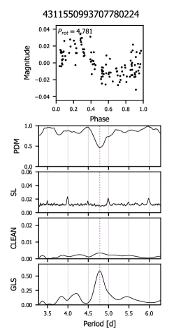
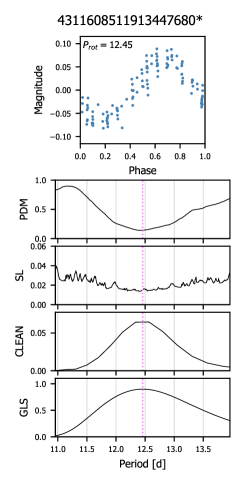
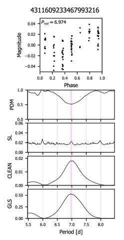
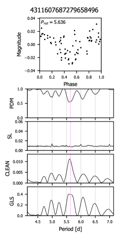
Figure 10: continued

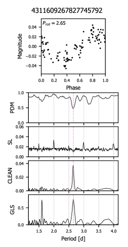
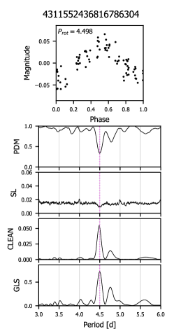
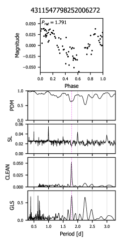
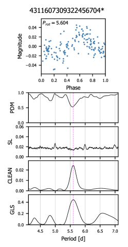
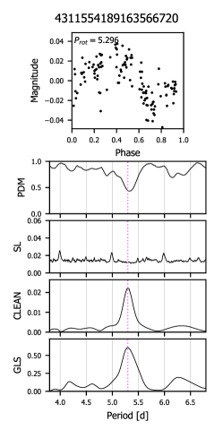
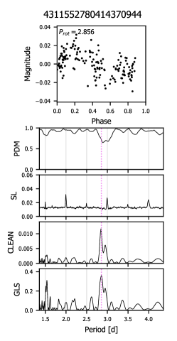
Figure 11: continued.

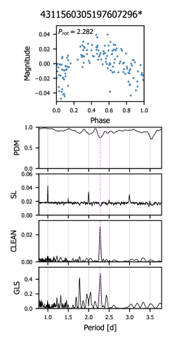
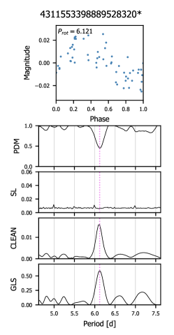
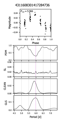
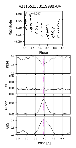
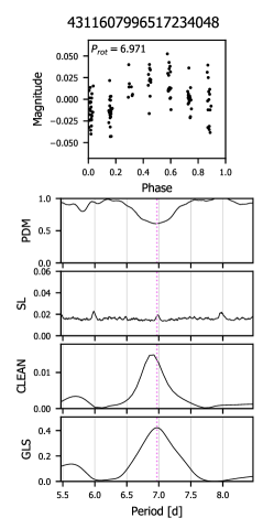
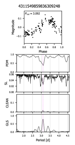
Figure 12: continued

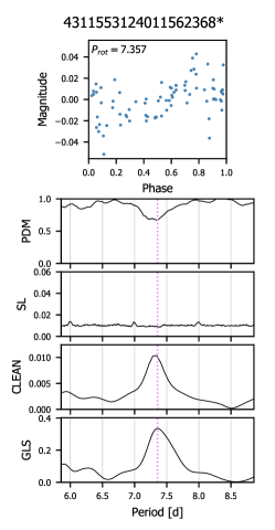
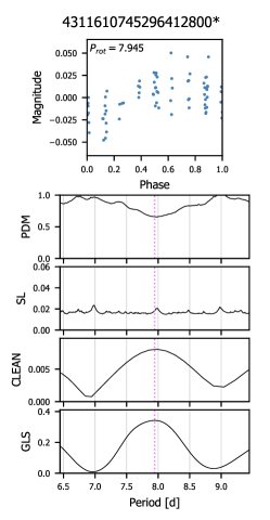
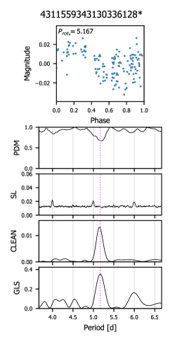
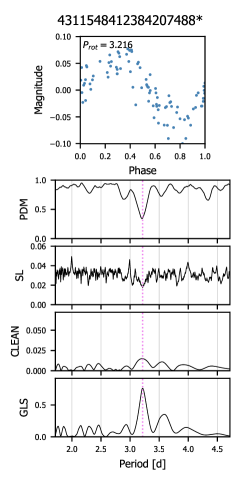
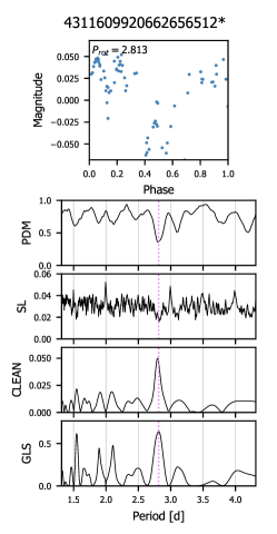
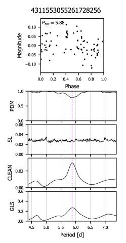
Figure 13: continued.

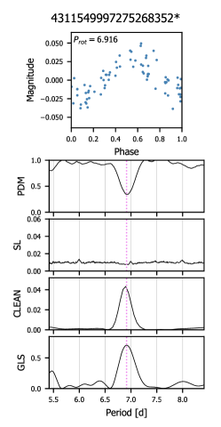
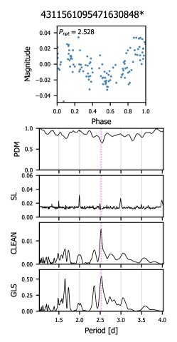
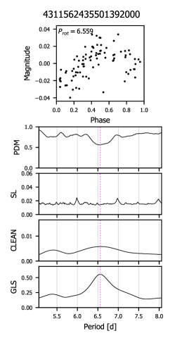
Figure 14: continued.