Context-aware controller inference for stabilizing dynamical systems from scarce data

Abstract

This work introduces a data-driven control approach for stabilizing high-dimensional dynamical systems from scarce data. The proposed context-aware controller inference approach is based on the observation that controllers need to act locally only on the unstable dynamics to stabilize systems. This means it is sufficient to learn the unstable dynamics alone, which are typically confined to much lower dimensional spaces than the high-dimensional state spaces of all system dynamics and thus few data samples are sufficient to identify them. Numerical experiments demonstrate that context-aware controller inference learns stabilizing controllers from orders of magnitude fewer data samples than traditional data-driven control techniques and variants of reinforcement learning. The experiments further show that the low data requirements of context-aware controller inference are especially beneficial in data-scarce engineering problems with complex physics, for which learning complete system dynamics is often intractable in terms of data and training costs.

1 Introduction

The design of feedback controllers for stabilizing dynamical systems is a ubiquitous task in science and engineering. Standard control techniques rely on the availability of models of the system dynamics to construct controllers. If models are unavailable, then typically models of system dynamics are learned from data first and then standard control techniques are applied to the learned models [7]. However, learning models of complex system dynamics can require large amounts of data because learning models means identifying generic descriptions that often also include information about the systems that are unnecessary for the specific task of finding stabilizing controllers. Additionally, collecting data from unstable systems is challenging because without a stabilizing controller the system cannot be observed for a long time before the dynamics become unstable and thus data collection becomes uninformative. In this work, we propose context-aware controller inference that stabilizes systems based on the unstable dynamics that are learned from few state observations by leveraging that unstable dynamics typically evolve in spaces of much lower dimension than the dimension of state spaces of all—stable and unstable—dynamics. We show that bases of the spaces of unstable dynamics can be efficiently estimated from derivative information of systems. The corresponding numerical procedure of context-aware controller inference achieves orders of magnitude reductions in the number of data samples that are required for finding stabilizing controllers compared to traditional data-driven methods that first identify models of the full dynamics that are subsequently stabilized.

Many approaches for model-free, data-driven controller design based on parameter tuning have been developed; see, e.g., [9, 13, 26, 43]. However, these methods are limited to systems with a small number of observables and inputs. In machine learning, reinforcement learning [48, 27, 39] has been successfully applied for the data-driven design of controllers, employing similar ideas as in the parameter tuning methods mentioned above. With the development of model reduction, efficient approaches for modeling reduced dynamical systems from data have been developed, such as dynamic mode decomposition and operator inference [45, 52, 38, 36, 51], sparse identification methods [8, 44], and the Loewner framework [29, 46, 37, 47, 2, 18]. These methods inform many data-driven controller techniques that first identify a model of the dynamics that is then stabilized by classical control approaches. However, it has been shown that less data are required for the task of stabilization than for the identification of models, which is the motivation for this work [11, 54, 57, 53].

We introduce context-aware controller inference, which is a new data-driven approach for learning stabilizing controllers from scarce data and that is applicable to systems with nonlinear dynamics. Context-aware controller inference exploits that controllers need to act only on the unstable parts of system dynamics for stabilization [4, 5, 21, 49] and that spaces in which the unstable dynamics evolve can be estimated efficiently and cheaply from gradients that are obtained from adjoints. If $r$ is the dimension of the space induced by the unstable dynamics, then there always exist $r$ states that are sufficient to be observed for inferring a feedback controller that is guaranteed to stabilize the system. The dimension $r$ of the space induced by the unstable dynamics is typically orders of magnitude lower than the dimension of the whole state space in which all dynamics evolve and which often determines the high data and training costs of traditional data-driven control methods. Context-aware controller inference thus opens the door to stabilizing systems from scarce data, such as near rare events and when data generation is expensive, even if systems describe complex physics.

2 Preliminaries

2.1 Stabilizing dynamical processes with feedback control

Consider a system that gives rise to a process $(x^{\mathrm{n}}(t))_{t\geq 0}$ that is controlled by inputs $(u^{\mathrm{n}}(t))_{t\geq 0}$, where $x^{\mathrm{n}}(t)\in\mathbb{R}^{N}$ and $u^{\mathrm{n}}(t)\in\mathbb{R}^{p}$ are the state and input at time $t$, respectively. The feasible initial conditions $x^{\mathrm{n}}(0)\in\mathcal{X}_{0}^{\mathrm{n}}$ are in the subspace $\mathcal{X}_{0}^{\mathrm{n}}\subset\mathbb{R}^{N}$. If the process is continuous in time, then the dynamics are governed by ordinary differential equations

$$\frac{\mathrm{d}}{\mathrm{d}t}x^{\mathrm{n}}(t) =f\big{(}x^{\mathrm{n}}(t),u^{\mathrm{n}}(t)\big{)}, t\geq 0,$$ (1)

with the potentially nonlinear right-hand side function $f\colon\mathbb{R}^{N}\times\mathbb{R}^{p}\rightarrow\mathbb{R}^{N}$. In discrete time, the process is governed by the difference equations

$$x^{\mathrm{n}}(t+1) =f\big{(}x^{\mathrm{n}}(t),u^{\mathrm{n}}(t)\big{)}, t\in\mathbb{N}_{0}:=\mathbb{N}\cup\{0\}.$$ (2)

Let $(\bar{x},\bar{u})\in\mathbb{R}^{N}\times\mathbb{R}^{p}$ be a controlled, constant-in-time steady state—equilibrium point—such that, in the continuous-time case,

$$f(\bar{x},\bar{u})=0,$$ (3)

and in the discrete-time case

$$f(\bar{x},\bar{u})=\bar{x}$$ (4)

hold. Conditions Eqs. 3 and 4 imply that the steady state is constant over time. In the following, we assume that the nonlinear function $f$ in Eqs. 1 and 2 is analytic at $(\bar{x},\bar{u})$.

A steady state $(\bar{x},\bar{u})$ is unstable if, for the fixed input signal $\bar{u}$, trajectories diverge away from $\bar{x}$ for initial conditions $x^{\mathrm{n}}(0)$ in a neighborhood of the steady state $\bar{x}$. A linear state-feedback controller $K\in\mathbb{R}^{p\times N}$ asymptotically stabilizes trajectories in sufficiently small neighborhoods about $\bar{x}$ if, for a given $x^{\mathrm{n}}(0)\in\mathcal{X}_{0}$ in a neighborhood of $\bar{x}$, the input trajectory $(u^{\mathrm{n}}(t))_{t\geq 0}$ with $u^{\mathrm{n}}(t)=K(x^{\mathrm{n}}(t)-\bar{x})+\bar{u}$ leads to $x^{\mathrm{n}}(t)\to\bar{x}$ for $t\to\infty$, where $(x^{\mathrm{n}}(t))_{t\geq 0}$ is given by either Eq. 1 or Eq. 2; see [33].

2.2 Problem formulation

In this work, a model of the system in form of the right-hand side function $f$ in Eq. 1 (or Eq. 2) is unavailable, which means the function $f$ cannot be evaluated directly and is not given in closed form. Instead, we either can generate data triplets $(U^{\mathrm{n}}_{-},X^{\mathrm{n}}_{-},X^{\mathrm{n}}_{+})$ by querying the system at feasible initial conditions and inputs in a black-box fashion or have given $(U^{\mathrm{n}}_{-},X^{\mathrm{n}}_{-},X^{\mathrm{n}}_{+})$. In the continuous-time case, the data triplets are

$$U^{\mathrm{n}}_{-} =\begin{bmatrix}u^{\mathrm{n}}(t_{0})&\ldots&u^{\mathrm{n}}(t_{T-1})\end{bmatrix}\in\mathbb{R}^{p\times T},\quad X^{\mathrm{n}}_{-}=\begin{bmatrix}x^{\mathrm{n}}(t_{0})&\ldots&x^{\mathrm{n}}(t_{T-1})\end{bmatrix}\in\mathbb{R}^{N\times T},$$

$$X^{\mathrm{n}}_{+} =\begin{bmatrix}\frac{\mathrm{d}}{\mathrm{d}t}x^{\mathrm{n}}(t_{0})&\ldots&\frac{\mathrm{d}}{\mathrm{d}t}x^{\mathrm{n}}(t_{T-1})\end{bmatrix}\in\mathbb{R}^{N\times T},$$

at discrete time points $0\leq t_{0}<t_{1}<\ldots<t_{T-1}$. In the discrete-time case, the data triplets are

$$U^{\mathrm{n}}_{-} =\begin{bmatrix}u^{\mathrm{n}}(0)&\ldots&u^{\mathrm{n}}(T-1)\end{bmatrix}\in\mathbb{R}^{p\times T},\quad X^{\mathrm{n}}_{-}=\begin{bmatrix}x^{\mathrm{n}}(0)&\ldots&x^{\mathrm{n}}(T-1)\end{bmatrix}\in\mathbb{R}^{N\times T},$$

$$X^{\mathrm{n}}_{+} =\begin{bmatrix}x^{\mathrm{n}}(1)&\ldots&x^{\mathrm{n}}(T)\end{bmatrix}\in\mathbb{R}^{N\times T}.$$

A data triplet $(U^{\mathrm{n}}_{-},X^{\mathrm{n}}_{-},X^{\mathrm{n}}_{+})$ can also contain the concatenation of several trajectories, which is not reflected in the notation for ease of exposition. We seek to construct controllers $K$ from data triplets $(U^{\mathrm{n}}_{-},X^{\mathrm{n}}_{-},X^{\mathrm{n}}_{+})$ to stabilize systems about steady states of interest $(\bar{x},\bar{u})$.

The traditional approach to data-driven control is first learning a model of the system dynamics and then applying standard techniques from control. However, this traditional two-step learn-then-stabilize approach can be expensive in terms of the number of required state observations, which typically scales with the dimension of the system [11, 54, 57, 53]. In particular, if observing states is expensive and the underlying dynamics describe complex physical phenomena, then often infeasibly high numbers of state observations are required to learn models of the system dynamics, which makes traditional learn-then-stabilize approaches intractable.

3 Inferring controllers from data of unstable dynamics

We introduce context-aware controller inference that guarantees learning stabilizing controllers with data requirements that scale as the dimension of the subspace spanned by the unstable dynamics, which is typically orders of magnitude lower than the dimension of the whole state space in which all dynamics evolve. To achieve this, we exploit that controllers need to act only on the unstable part of the system dynamics for stabilization.

3.1 Stabilizing nonlinear systems near steady states

Let $(\bar{x},\bar{u})$ be a steady state. The right-hand side function $f$ of Eq. 1 (or Eq. 2) can be approximated at $(x^{\mathrm{n}}(t),u^{\mathrm{n}}(t))$ with the first two terms of its Taylor series expansion about $(\bar{x},\bar{u})$:

$$f\big{(}x^{\mathrm{n}}(t),u^{\mathrm{n}}(t)\big{)}=f(\bar{x},\bar{u})+\partial_{\mathrm{x}}f(\bar{x},\bar{u})\big{(}x^{\mathrm{n}}(t)-\bar{x}\big{)}+\partial_{\mathrm{u}}f(\bar{x},\bar{u})\big{(}u^{\mathrm{n}}(t)-\bar{u}\big{)}$$ (5)

$${}+{}\mathcal{O}\left(\big{(}x^{\mathrm{n}}(t)-\bar{x}\big{)}^{2}\right)+\mathcal{O}\left(\big{(}u^{\mathrm{n}}(t)-\bar{u}\big{)}^{2}\right),$$

where $\partial_{\mathrm{x}}f(\bar{x},\bar{u})$ and $\partial_{\mathrm{u}}f(\bar{x},\bar{u})$ denote the parts of the Jacobian at $(\bar{x},\bar{u})$ of $f$ with respect to $x^{\mathrm{n}}(t)$ and $u^{\mathrm{n}}(t)$, respectively. The first term $f(\bar{x},\bar{u})$ in Eq. 5 is either $f(\bar{x},\bar{u})=0$ or $f(\bar{x},\bar{u})=\bar{x}$; cf. Equations 3 and 4. With the system matrices $A=\partial_{\mathrm{x}}f(\bar{x},\bar{u})\in\mathbb{R}^{N\times N}$ and $B=\partial_{\mathrm{u}}f(\bar{x},\bar{u})\in\mathbb{R}^{N\times p}$, a model of the linearized system of Eq. 1 about the steady state is

$$\frac{\mathrm{d}}{\mathrm{d}t}x(t) =Ax(t)+Bu(t), t\geq 0,$$ (6)

and analogously for the discrete-time case Eq. 2,

$$x(t+1) =Ax(t)+Bu(t), t\in\mathbb{N}_{0},$$ (7)

where $x(t)$ approximates the shifted nonlinear state $x^{\mathrm{n}}(t)-\bar{x}$ at time $t$ and the input $u(t)$ corresponds to $u^{\mathrm{n}}(t)-\bar{u}$.

The system described by the model Eq. 6 (or Eq. 7) is called asymptotically stabilizable if there exists a constant matrix $K\in\mathbb{R}^{p\times N}$ such that the application of the state feedback $u(t)=Kx(t)$ stabilizes the system, i.e., $\lVert x(t)\rVert\rightarrow 0$ for $t\rightarrow\infty$. A linear model such as Eq. 6 is asymptotically stable if all eigenvalues of $A$ have negative real parts; in case of discrete-time linear models Eq. 7, the eigenvalues of $A$ have to be inside the unit disc. A linear state-space model is called stabilizable if there exists a $K$ such that $A+BK$ has only stable eigenvalues.

The following proposition states that a controller $K$ obtained from the linearized system is guaranteed to stabilize the nonlinear system if the state $x^{\mathrm{n}}(t)$ stays in the neighborhood of the steady state $\bar{x}$.

Proposition 1 (Locally stabilizing feedback controller; cf. [33, Sec. 10.1]).

Consider a linearized system described by Eq. 6 (or Eq. 7) of a corresponding nonlinear system described by Eq. 1 (or Eq. 2) at the steady state of interest $(\bar{x},\bar{u})$, where the nonlinear function $f$ is analytic. If $K$ is a controller that stabilizes the linearized system asymptotically, then $u^{\mathrm{n}}(t)=K(x^{\mathrm{n}}(t)-\bar{x})+\bar{u}$ locally stabilizes the nonlinear system about $(\bar{x},\bar{u})$ in the asymptotic sense, i.e., there exists an $\epsilon>0$ such that for all $x^{\mathrm{n}}(0)\in\mathcal{X}_{0}^{\mathrm{n}}(0)$ with $\lVert\bar{x}-x^{\mathrm{n}}(0)\rVert<\epsilon$ we have that $x^{\mathrm{n}}(t)\rightarrow\bar{x}$ for $t\rightarrow\infty$.

3.2 Stabilizing models based on unstable eigenvalues

To restrict the action of a controller $K$ to the unstable eigenvalues of the spectrum of linear models, we build on the theory of pole placement [55, 42] and partial stabilization [4, 5, 21, 49]. This leads to a reduction of the dimension of the spaces in which the dynamics evolve, from a typically high-dimensional state space to subspaces spanned by the unstable dynamics that are often orders of magnitude lower in dimension. In this section, we generalize concepts of partial stabilization to be applicable to the data-driven setting.

In the following, when we state that two matrices have the same spectrum, it implies that they have the same eigenvalues with the same geometric and algebraic multiplicities.

Lemma 1.

Consider the linear model $(A,B)$ given in Eq. 6 (or Eq. 7) and assume it is stabilizable. Let $W\in\mathbb{R}^{N\times n_{\mathrm{u}}}$ be a basis matrix of the $n_{\mathrm{u}}$-dimensional left eigenspace of $A$ corresponding to the unstable eigenvalues and define the matrices

$$\widehat{A} =W^{\mkern-1.5mu\mathsf{T}}A\left(W^{\dagger}\right)^{\mkern-1.5mu\mathsf{T}}, \widehat{B} =W^{\mkern-1.5mu\mathsf{T}}B,$$ (8)

where $W^{\dagger}$ is a left inverse of $W$. Let further $\widehat{K}$ stabilize $(\widehat{A},\widehat{B})$. Then, it holds that

$$K=\widehat{K}W^{\mkern-1.5mu\mathsf{T}}$$

stabilizes the model $(A,B)$. Furthermore, it holds that the spectrum of $\widehat{A}$ is the spectrum of $A$ corresponding to the unstable eigenvalues and that the union of the stable spectrum of $A$ and the spectrum of $\widehat{A}+\widehat{B}\widehat{K}$ is the spectrum of $A+BK$.

Lemma 1 implies that the unstable dynamics of the model $(A,B)$ can be fully described by the space spanned by the columns of the basis matrix $W$, which contains as columns the left eigenvectors of the unstable eigenvalues of $A$. The eigenvalues of $A$ can be complex such that also the corresponding eigenvectors are complex-valued. However, with the assumption that $A$ is real-valued, the eigenvalues and eigenvectors appear in complex conjugate pairs such that there exists a real basis matrix $W$ of the corresponding complex eigenspace; see, e.g., [17, Sec. 7.4.1]. The last statement of Lemma 1 implies that only the unstable eigenvalues of $A$ are changed in the closed-loop model by the application of $K$. In particular, the eigenvalues are determined via the spectrum of the reduced closed-loop model $\widehat{A}+\widehat{B}\widehat{K}$ by the construction of $\widehat{K}$.

Proof of Lemma 1..

A basis matrix $\widetilde{W}\in\mathbb{C}^{N\times n_{\mathrm{u}}}$ of the left eigenspace of $A$ corresponding to the unstable eigenvalues is defined by

$$A^{\mkern-1.5mu\mathsf{T}}\widetilde{W}=\widetilde{W}\Lambda^{\mkern-1.5mu\mathsf{T}},$$ (9)

where $\Lambda\in\mathbb{C}^{n_{\mathrm{u}}\times n_{\mathrm{u}}}$ consists of Jordan blocks with the unstable eigenvalues of $A$ on its diagonal. There exists a transformation $S\in\mathbb{C}^{n_{\mathrm{u}}\times n_{\mathrm{u}}}$ with $\Lambda=S^{-1}\widehat{A}S$, where $\widehat{A}$ is from Eq. 8, such that $\widehat{A}$ has by construction the same spectrum as $\Lambda$. Inserting the transformation into Eq. 9 yields

$$A^{\mkern-1.5mu\mathsf{T}}\widetilde{W} =\widetilde{W}S^{\mkern-1.5mu\mathsf{T}}\widehat{A}^{\mkern-1.5mu\mathsf{T}}S^{-\mkern-1.5mu\mathsf{T}} \Leftrightarrow A^{\mkern-1.5mu\mathsf{T}}\widetilde{W}S^{\mkern-1.5mu\mathsf{T}} =\widetilde{W}S^{\mkern-1.5mu\mathsf{T}}\widehat{A}^{\mkern-1.5mu\mathsf{T}}.$$

Setting $W=\widetilde{W}S^{\mkern-1.5mu\mathsf{T}}$ and transposing the eigenvalue relation we see that

$$\widehat{A}=W^{\mkern-1.5mu\mathsf{T}}A\left(W^{\dagger}\right)^{\mkern-1.5mu\mathsf{T}}$$ (10)

holds for any left inverse $W^{\dagger}$ of $W$. Let $W_{\perp}$ be a basis matrix of the orthogonal complement to the subspace spanned by the columns of $W$, i.e., it holds that

$$\operatorname{span}\left(\begin{bmatrix}W&W_{\perp}\end{bmatrix}\right)=\mathbb{R}^{N},$$

with $W_{\perp}^{\mkern-1.5mu\mathsf{T}}W=0$ and $W^{\mkern-1.5mu\mathsf{T}}W_{\perp}=0$. Then, it holds that

$$\begin{bmatrix}W&W_{\perp}\end{bmatrix}^{\mkern-1.5mu\mathsf{T}}A\begin{bmatrix}W&W_{\perp}\end{bmatrix}^{-\mkern-1.5mu\mathsf{T}} =\begin{bmatrix}\widehat{A}&0\\ A_{21}&A_{22}\end{bmatrix}, \begin{bmatrix}W&W_{\perp}\end{bmatrix}^{\mkern-1.5mu\mathsf{T}}B =\begin{bmatrix}\widehat{B}\\ B_{2}\end{bmatrix},$$ (11)

where $\widehat{B}$ is as in Eq. 8 and the spectrum of $A_{22}$ is the stable spectrum of $A$; see, e.g., [17, Thm. 7.1.6]. We can now construct a controller $\widehat{K}$ such that $\widehat{A}+\widehat{B}\widehat{K}$ is stable since $(A,B)$ has been assumed to be stabilizable. Augmenting the controller $\widehat{K}$ by zeros yields the closed-loop matrix of Eq. 11 as

$$\begin{bmatrix}\widehat{A}&0\\ A_{21}&A_{22}\end{bmatrix}+\begin{bmatrix}\widehat{B}\\ B_{2}\end{bmatrix}\begin{bmatrix}\widehat{K}&0\end{bmatrix}=\begin{bmatrix}\widehat{A}+\widehat{B}\widehat{K}&0\\ A_{21}+B_{2}\widehat{K}&A_{22}\end{bmatrix}.$$ (12)

The closed-loop matrix in Eq. 12 is stable since $\widehat{K}$ has been chosen such that $\widehat{A}+\widehat{B}\widehat{K}$ is stable and $A_{22}$ has only stable eigenvalues. Inverting the transformation in Eq. 11 and applying that to Eq. 12 gives the closed-loop matrix of the original state-space model with

$$A+BK=\begin{bmatrix}W&W_{\perp}\end{bmatrix}^{-\mkern-1.5mu\mathsf{T}}\left(\begin{bmatrix}\widehat{A}&0\\ A_{21}&A_{22}\end{bmatrix}+\begin{bmatrix}\widehat{B}\\ B_{2}\end{bmatrix}\begin{bmatrix}\widehat{K}&0\end{bmatrix}\right)\begin{bmatrix}W&W_{\perp}\end{bmatrix}^{\mkern-1.5mu\mathsf{T}},$$

which reveals by multiplying out the block matrices that

$$K=\begin{bmatrix}\widehat{K}&0\end{bmatrix}\begin{bmatrix}W&W_{\perp}\end{bmatrix}^{\mkern-1.5mu\mathsf{T}}=\widehat{K}W^{\mkern-1.5mu\mathsf{T}}$$

holds. Since transformations do not change the spectrum of matrices, the spectrum of $A+BK$ is the spectrum of Eq. 12, which concludes the proof. ∎

In Lemma 1, the left eigenvector basis is essential for the proof. It leads to the lower triangular form Eq. 11 that has the required ordering of the diagonal blocks with the unstable eigenvalues contained in the upper and the stable eigenvalues in the lower diagonal block. This particular ordering is necessary since otherwise the spectrum is disturbed by the action of the controller; cf. [57, Sec. 3.2.2]. However, the left eigenspace of the unstable eigenvalues can also be constructed as orthogonal complement of the right eigenspace of the stable eigenvalues, as the next lemma shows.

Lemma 2.

Given a matrix $A$, let $W\in\mathbb{R}^{N\times n_{\mathrm{u}}}$ be a basis matrix of the left eigenspace corresponding to the unstable eigenvalues of $A$, and let $Q_{\perp}\in\mathbb{R}^{N\times n_{\mathrm{u}}}$ be a basis matrix of the orthogonal complement to the right eigenspace of $A$ corresponding to the stable eigenvalues. Then, it holds that

$$\operatorname{span}(W)=\operatorname{span}\left(\left(Q_{\perp}^{\dagger}\right)^{\mkern-1.5mu\mathsf{T}}\right),$$ (13)

for all left inverses $Q_{\perp}^{\dagger}$ of $Q_{\perp}$. In the case $Q_{\perp}$ is an orthogonal basis, Equation 13 simplifies to

$$\operatorname{span}(W)=\operatorname{span}(Q_{\perp}).$$

Proof.

Let $Q$ be a basis matrix of the eigenspace of $A$ associated with the stable eigenvalues. By basis concatenation with $Q_{\perp}$, it holds

$$\begin{bmatrix}Q_{\perp}&Q\end{bmatrix}^{-1}A\begin{bmatrix}Q_{\perp}&Q\end{bmatrix}=\begin{bmatrix}\widehat{A}&0\\ A_{21}&A_{22}\end{bmatrix},$$ (14)

where the spectrum of $\widehat{A}$ is the unstable spectrum of $A$ and the spectrum of $A_{22}$ is the stable one of $A$; see [17, Thm. 7.1.6]. In particular, we get from Eq. 14 that

$$Q_{\perp}^{\dagger}AQ_{\perp}=\widehat{A},$$ (15)

for all left inverses $Q_{\perp}^{\dagger}$ of $Q_{\perp}$. The basis matrix $W$ can be chosen such that the matrices $\widehat{A}$ and $A_{22}$ in Eqs. 11 and 14 are identical, since both spectra are identical there must be an appropriate similarity transformation. Comparing the two basis matrices in Eqs. 15 and 10 yields the result. ∎

Note that there is a line of work on constructing manifolds of unstable dynamics, instead of subspaces as in our approach. Working with manifolds, instead of spaces, can potentially be beneficial when systems are strongly nonlinear. The corresponding computational methods involving manifolds can become computationally challenging, especially for systems in high-dimensional state spaces [24, 59]. It remains future work to efficiently combine our control approach with methods for constructing unstable manifolds.

3.3 Controller inference from idealized data

In this section, we will construct stabilizing controllers from given data triplets. For now, we consider data triplets $(U_{-},X_{-},X_{+})$ that are idealized in the sense that they are obtained from models of the linearized systems. However, in the next section and in the numerical experiments we will consider data from the original nonlinear systems. In the continuous-time case, the idealized data triplets are

$$U_{-} =\begin{bmatrix}u(t_{0})&\dots&u(t_{T-1})\end{bmatrix}, X_{-} =\begin{bmatrix}x(t_{0})&\dots&x(t_{T-1})\end{bmatrix},$$

$$X_{+} =\begin{bmatrix}\frac{\mathrm{d}}{\mathrm{d}t}x(t_{0})&\dots&\frac{\mathrm{d}}{\mathrm{d}t}x(t_{T-1})\end{bmatrix},$$

at discrete time points $0\leq t_{0}<t_{1}<\ldots<t_{T-1}$ with states from Eq. 6, and in the discrete-time case, the idealized data triplets with states from Eq. 7 are

$$U_{-} =\begin{bmatrix}u(0)&\dots&u(T-1)\end{bmatrix}, X_{-} =\begin{bmatrix}x(0)&\dots&x(T-1)\end{bmatrix},$$

$$X_{+} =\begin{bmatrix}x(1)&\dots&x(T)\end{bmatrix}.$$

The fundamental principle of data informativity [54] is that potentially many linear models can describe a given data triplet $(U_{-},X_{-},X_{+})$ and that a stabilizing controller needs to stabilize all those linear models to guarantee the stabilization of the model from which the data has been generated. The set of all linear models that explain $(U_{-},X_{-},X_{+})$ is

$$\Sigma_{\mathrm{i/s}}=\left\{(A,B)\left|\leavevmode\nobreak\ X_{+}=AX_{-}+BU_{-}\right.\right\},$$

and all linear models that are stabilized by a given $K$ are

$$\Sigma_{K}=\left\{(A,B)\left|\leavevmode\nobreak\ A+BK\leavevmode\nobreak\ \text{is stable}\right.\right\}.$$

A given data triplet $(U_{-},X_{-},X_{+})$ is called informative for stabilization if there exists a controller $K$ that stabilizes all explaining linear models, which means in terms of the two sets $\Sigma_{\mathrm{i/s}}$ and $\Sigma_{\mathrm{K}}$ that $\Sigma_{\mathrm{i/s}}\subseteq\Sigma_{\mathrm{K}}$ holds; see [54].

The matrix $A$ of the linear model $(A,B)$ can have components corresponding to unstable eigenvalues that do not contribute to the system dynamics, which means these are not excited by initial conditions from $\mathcal{X}_{0}$ or the system inputs. For any linear model $(A,B)$ with a basis matrix $X_{0}$ of the initial conditions subspace $\mathcal{X}_{0}$, there exists an invertible matrix $S\in\mathbb{R}^{N\times N}$ to transform the system into the Kalman controllability form:

$$S^{-1}AS =\begin{bmatrix}A_{11}&A_{12}&A_{13}\\ 0&A_{22}&A_{23}\\ 0&0&A_{33}\end{bmatrix}, S^{-1}B =\begin{bmatrix}B_{1}\\ 0\\ 0\end{bmatrix}, S^{-1}X_{0} =\begin{bmatrix}X_{10}\\ X_{20}\\ 0\end{bmatrix},$$ (16)

where the zero blocks in the transformed $B$ and $X_{0}$ are chosen as large as possible; see [57]. The first block row in Eq. 16 corresponds to the controllable dynamics, the second one to those only excited by the initial conditions and the last block row are zero dynamics, which are neither excited by inputs nor initial conditions. Consequently, the eigenspaces corresponding to the unstable eigenvalues in $A_{33}$ do not result in unstable dynamics since these components are never excited. In the following, we consider the left eigenbasis matrix $W\in\mathbb{R}^{N\times r}$ to be minimal in the sense that the subspace $\mathcal{W}$ spanned by $W$ contains the left eigenspaces corresponding to the unstable eigenvalues in $A_{11}$ and $A_{22}$ in Eq. 16. If $A_{33}$ has unstable eigenvalues, the corresponding eigenbasis is not taken into account. In other words, we consider only those eigenspaces that describe unstable dynamics that can be excited by initial conditions or inputs.

The following theorem characterizes the stabilization of models based on unstable dynamics using the data informativity concept.

Theorem 1.

Consider a potentially nonlinear system given by Eq. 1 (or Eq. 2). Given $(U_{-},X_{-},X_{+})$ a data triplet sampled from a linearized model obtained from the considered nonlinear system about the steady state $(\bar{x},\bar{u})$, with state-space dimension $N$. Let further $W\in\mathbb{R}^{N\times r}$ be a basis matrix of the minimal left eigenspace of the unstable eigenvalues that correspond to the unstable system dynamics. If the data triplet $(U_{-},\widehat{X}_{-},\widehat{X}_{+})$ is informative for stabilization, which means that $\widehat{\Sigma}_{\mathrm{i/s}}\subseteq\widehat{\Sigma}_{\widehat{K}}$ holds for a suitable $\widehat{K}\in\mathbb{R}^{p\times r}$ and

$$\widehat{X}_{-} =W^{\mkern-1.5mu\mathsf{T}}X_{-} \widehat{X}_{+} =W^{\mkern-1.5mu\mathsf{T}}X_{+},$$ and (17)

then the controller $K=\widehat{K}W^{\mkern-1.5mu\mathsf{T}}$ stabilizes the linearized system and is also locally stabilizing the steady state $(\bar{x},\bar{u})$ of the nonlinear system in the sense of Proposition 1.

Proof of Theorem 1..

Let $(A,B)$ be the linear model from which the data $(U_{-},X_{-},X_{+})$ has been sampled. Because the columns of $W$ span the eigenspace of unstable eigenvalues, it holds that

$$W^{\mkern-1.5mu\mathsf{T}}A\left(W^{\dagger}\right)^{\mkern-1.5mu\mathsf{T}} =\widehat{A}, W^{\mkern-1.5mu\mathsf{T}}B =\widehat{B} W^{\mkern-1.5mu\mathsf{T}}X_{0} =\widehat{X}_{0},$$ and (18)

where the spectrum of $\widehat{A}$ is the unstable spectrum of $A$ that contributes to the system dynamics and $X_{0}$ is a basis of the subspace of initial conditions $\mathcal{X}_{0}$. For the reduced data in Eq. 17 it holds that

$$\widehat{X}_{+}=W^{\mkern-1.5mu\mathsf{T}}X_{+}=W^{\mkern-1.5mu\mathsf{T}}AX_{-}+W^{\mkern-1.5mu\mathsf{T}}BU_{-}=\widehat{A}W^{\mkern-1.5mu\mathsf{T}}X_{-}+\widehat{B}U_{-}=\widehat{A}\widehat{X}_{-}+\widehat{B}U_{-}.$$ (19)

Thus, $(\widehat{A},\widehat{B})$ is a model that explains the data $(U_{-},\widehat{X}_{-},\widehat{X}_{+})$. Since the nonlinear system is assumed to be stabilizable, this holds for the linearized model, too. Since $(U_{-},\widehat{X}_{-},\widehat{X}_{+})$ from Eq. 17 is informative for stabilization, there is a $\widehat{K}$ such that $\widehat{\Sigma}_{\mathrm{i/s}}\subseteq\widehat{\Sigma}_{\widehat{K}}$. Together with Eq. 19, the feedback $\widehat{K}$ stabilizes also the linear model $(\widehat{A},\widehat{B})$ from Eq. 18. The unstable eigenvalues of the high-dimensional $A$ that do not contribute to the system dynamics can be replaced by stable eigenvalues as it does not change the dynamics and consequently the given data; see, e.g., [57]. Therefore, one can assume $(A,B)$ to be stabilizable. From Lemma 1 it follows that $K=\widehat{K}W^{\mkern-1.5mu\mathsf{T}}$ stabilizes $(A,B)$, which means it stabilizes the linearized system. Since $K$ stabilizes a linearized system of a nonlinear process about the steady state $(\bar{x},\bar{u})$, it follows from Proposition 1 that it also stabilizes the nonlinear process locally at $(\bar{x},\bar{u})$, which concludes the proof. ∎

It has been shown in [57, Cor. 3 and 4] that the minimum number of state observations required for stabilizing all low-dimensional linear systems explaining a given data triplet scales with the intrinsic, minimal state-space dimension of the underlying system that is described by the model from which data were obtained. Building on the data reduction in Eq. 17 in Theorem 1, the following corollary shows that the restriction to the unstable dynamics in $\mathcal{W}$ can further reduce the number of required state observations to $r$, the dimension of $\mathcal{W}$.

Corollary 1.

Let Theorem 1 apply and let $r$ be the number of excitable unstable eigenvalues of the linear model corresponding to the nonlinear system. Then, there always exist $r$ states of the linear model that are sufficient to be observed for inferring a guaranteed locally stabilizing controller for the nonlinear system, even if high-dimensional states of dimension $N\gg r$ are observed.

The number of state observations $r$ in Corollary 1 for constructing a guaranteed stabilizing controller for the nonlinear system does neither scale with the large state dimension $N$ nor with the intrinsic system dimension $n_{\min}$. In fact, $r$ is typically orders of magnitude smaller than $N$ and $n_{\min}$. However, there is a certain price that needs to be paid for the application of Theorems 1 and 1: A basis matrix $W$ (or alternatively $Q_{\perp}$ from Lemma 2) must be available. Approaches for the computation of $W$ (or $Q_{\perp}$) from data are discussed in Section 4.

3.4 Computational approach for controller inference

This section introduces a computational approach for context-aware controller inference that is motivated by the theoretical considerations of the previous sections. We now consider data $(U^{\mathrm{n}}_{-},X^{\mathrm{n}}_{-},X^{\mathrm{n}}_{+})$ from the nonlinear system rather than idealized data $(U_{-},X_{-},X_{+})$ as in the previous section. The computational procedure is summarized in Algorithm 1.

1

Input: Data triplet $(U^{\mathrm{n}}_{-},X^{\mathrm{n}}_{-},X^{\mathrm{n}}_{+})$, steady state $(\bar{x},\bar{u})$, basis matrix $\widetilde{W}\in\mathbb{R}^{N\times n_{\mathrm{u}}}$ of the left eigenspace $\mathcal{W}$ corresponding to the unstable eigenvalues of the linear model.

Output: Controller $K$.

2

3Shift $(U^{\mathrm{n}}_{-},X^{\mathrm{n}}_{-},X^{\mathrm{n}}_{+})$ by the steady state $(\bar{x},\bar{u})$ to obtain $(\breve{U}_{-},\breve{X}_{-},\breve{X}_{+})$ via Eq. 20 (or Eq. 21).

4

5Project onto the left eigenspace $\widetilde{\mathcal{W}}$ so that only the unstable dynamics in the data remain

$$\widetilde{X}_{-} =\widetilde{W}^{\mkern-1.5mu\mathsf{T}}\breve{X}_{-} \widetilde{X}_{+} =\widetilde{W}^{\mkern-1.5mu\mathsf{T}}\breve{X}_{+}.$$ and

6

7Derive the basis matrix $V\in\mathbb{R}^{n_{\mathrm{u}}\times r}$ of $\mathcal{V}$ using the singular value decomposition

$$\begin{bmatrix}\widetilde{X}_{-}&\widetilde{X}_{+}\end{bmatrix}=\begin{bmatrix}V&V_{2}\end{bmatrix}\begin{bmatrix}\Sigma_{1}&0\\ 0&0\end{bmatrix}U^{\mkern-1.5mu\mathsf{T}}.\;$$

8Project onto $\mathcal{V}$ so that only unstable and excitable dynamics remain

$$\widehat{X}_{-} =V^{\mkern-1.5mu\mathsf{T}}\widetilde{X}_{-} \widehat{X}_{+} =V^{\mkern-1.5mu\mathsf{T}}\widetilde{X}_{+}.$$ and

9

10Compute the eigenbasis matrix $W=\widetilde{W}V$ of the minimal subspace of unstable dynamics.

11

12Infer a low-dimensional stabilizing controller $\widehat{K}=\breve{U}_{-}\Theta(\widehat{X}_{-}\Theta)^{-1}$ from $\breve{U}_{-},\widehat{X}_{-},$ and $\widehat{X}_{+}$ by solving Eq. 22 (or Eq. 23) for the unknown $\Theta$.

13

14Lift the inferred low-dimensional controller $\widehat{K}$ to

$$K=\widehat{K}W^{\mkern-1.5mu\mathsf{T}}.$$

Algorithm 1 Context-aware controller inference

In Step 1 of Algorithm 1, the data $(U^{\mathrm{n}}_{-},X^{\mathrm{n}}_{-},X^{\mathrm{n}}_{+})$ from the nonlinear system are shifted as

$$\breve{U}_{-} =\begin{bmatrix}u^{\mathrm{n}}(t_{0})-\bar{u}&\ldots&u^{\mathrm{n}}(t_{T-1})-\bar{u}\end{bmatrix},\quad\breve{X}_{-}=\begin{bmatrix}x^{\mathrm{n}}(t_{0})-\bar{x}&\ldots&x^{\mathrm{n}}(t_{T-1})-\bar{x}\end{bmatrix},$$ (20)

$$\breve{X}_{+} =\begin{bmatrix}\frac{\mathrm{d}}{\mathrm{d}t}x^{\mathrm{n}}(t_{0})&\ldots&\frac{\mathrm{d}}{\mathrm{d}t}x^{\mathrm{n}}(t_{T-1})\end{bmatrix},$$

in the continuous-time case and

$$\breve{U}_{-} =\begin{bmatrix}u^{\mathrm{n}}(0)-\bar{u}&\ldots&u^{\mathrm{n}}(T-1)-\bar{u}\end{bmatrix},\quad\breve{X}_{-}=\begin{bmatrix}x^{\mathrm{n}}(0)-\bar{x}&\ldots&x^{\mathrm{n}}(T-1)-\bar{x}\end{bmatrix},$$ (21)

$$\breve{X}_{+} =\begin{bmatrix}x^{\mathrm{n}}(1)-\bar{x}&\ldots&x^{\mathrm{n}}(T)-\bar{x}\end{bmatrix},$$

in the discrete-time case. The shifted data Eqs. 20 and 21 are related to the idealized data $(U_{-},X_{-},X_{+})$, which are used in Section 3.3, as

$$U_{-}=\breve{U}_{-},\quad X_{-}=\breve{X}_{-}+\mathcal{O}\left((X^{\mathrm{n}}_{-}-\bar{x})^{2}\right),\quad X_{+}=\breve{X}_{+}+\mathcal{O}\left((X^{\mathrm{n}}_{+}-\bar{x})^{2}\right)+\mathcal{O}\left((U^{\mathrm{n}}_{+}-\bar{u})^{2}\right),$$

which holds because of the Taylor approximation Eq. 5 and shows that data from the nonlinear system are close to the idealized data if trajectories stay within a small neighborhood of $(\bar{x},\bar{u})$.

Step 1 of Algorithm 1 projects the shifted data onto the subspace of unstable dynamics $\mathcal{W}$ so that only the unstable parts of the trajectories remain in $\widetilde{X}_{-}$ and $\widetilde{X}_{+}$. The basis matrix $\widetilde{W}$ may not span the minimal subspace of unstable dynamics as required by Theorem 1, i.e., the subspace $\widetilde{\mathcal{W}}$ contains an eigenspace of $A$ corresponding to zero dynamics; cf. the third block row in Eq. 16. This can be the case when $\widetilde{W}$ is computed as shown in the next section. The zero dynamics lead to a smaller minimal system dimension $r<n_{\mathrm{u}}$ and rank deficient data matrices $\widetilde{X}_{-}$ and $\widetilde{X}_{+}$. Any rank revealing decomposition of the data can be used to remove their kernel and reduce the eigenspace to the requested minimal subspace. In Step 7, the singular value decomposition is used for this purpose. Then the data is projected onto the minimal subspace of unstable dynamics in Step 1 and the corresponding basis matrix is computed in Step 1.

Step 1 of Algorithm 1 infers a controller from the unstable and excitable dynamics in $\widehat{X}_{-}$ and $\widehat{X}_{+}$. The controller is given by $\widehat{K}=\breve{U}_{-}\Theta(X_{-}\Theta)^{-1}$, where $\Theta\in\mathbb{R}^{T\times r}$ solves, in the continuous-time case,

$$\widehat{X}_{-}\Theta >0 \widehat{X}_{+}\Theta+\Theta^{\mkern-1.5mu\mathsf{T}}\widehat{X}_{+}^{\mkern-1.5mu\mathsf{T}}<0$$ and (22)

and in the discrete-time case

$$\widehat{X}_{-}\Theta =(\widehat{X}_{-}\Theta)^{\mkern-1.5mu\mathsf{T}} \begin{bmatrix}\widehat{X}_{-}\Theta&\widehat{X}_{+}\Theta\\ (\widehat{X}{+}\Theta)^{\mkern-1.5mu\mathsf{T}}&\widehat{X}_{-}\Theta\end{bmatrix}>0;$$ and (23)

see [57, 54, 11].

In the last step of Algorithm 1, the inferred controller $\widehat{K}$ is lifted to the original state-space dimension $K=\widehat{K}W^{\mkern-1.5mu\mathsf{T}}$ such that $u^{\mathrm{n}}(t)=K(x^{\mathrm{n}}(t)-\bar{x}(t))+\bar{u}(t)$ stabilizes the nonlinear system under the assumptions given in Proposition 1.

In Algorithm 1, the stabilizing controller is inferred from $\widehat{X}_{-}$ and $\widehat{X}_{+}$ by solving the linear matrix inequalities Eqs. 22 and 23, respectively. If the number of observed states $T$ equals the dimension $r$ of the unstable dynamics, then a computationally more efficient alternative to solving Eqs. 22 and 23 is introduced in [54, Thm. 16] and [57, Prp. 2 and Cor. 1]. It computes only the inverse of the reduced data matrix $\widehat{X}_{-}$. Also, to identify a model that describes the unstable system dynamics, Step 1 can be replaced by [57, Prp. 1]. With the identified model describing the unstable dynamics, classical stabilization approaches can be employed to compute a suitable $\widehat{K}$.

Note that the system needs to be stabilizable for the matrix inequalities Eqs. 22 and 23 to be solvable. If the system is not stabilizable, the inequalities have no solution and the solvers employed in Step 1 of Algorithm 1 throw an error that no stabilizing controller can be inferred.

4 Estimating left eigenspaces from gradient samples

In this section, we discuss leveraging samples of gradients to estimate a basis matrix $W$ of the left eigenspace $\mathcal{W}$ of unstable eigenvalues. Let

$$F(x^{\mathrm{n}}(t),u^{\mathrm{n}}(t)):=\frac{\mathrm{d}}{\mathrm{d}t}x^{\mathrm{n}}(t)-f\big{(}x^{\mathrm{n}}(t),u^{\mathrm{n}}(t)\big{)}$$ (24)

denote the residual formulation of the continuous-time model Eq. 1. The transposed gradient of Eq. 24 at the steady state $(\bar{x},\bar{u})$ is

$$\mathcal{F}[\bar{x},\bar{u}]:=\Big{(}\partial_{\mathrm{x}}F\big{(}\bar{x},\bar{u}\big{)}\Big{)}^{\mkern-1.5mu\mathsf{T}}=\left(\partial_{\mathrm{x}}\frac{\mathrm{d}}{\mathrm{d}t}\bar{x}\right)^{\mkern-1.5mu\mathsf{T}}-\big{(}\partial_{\mathrm{x}}f(\bar{x},\bar{u})\big{)}^{\mkern-1.5mu\mathsf{T}}=-A^{\mkern-1.5mu\mathsf{T}},$$ (25)

which can be applied to a vector $x$ as

$$\mathcal{F}[\bar{x},\bar{u}](x):=-A^{\mkern-1.5mu\mathsf{T}}x,$$ (26)

where $A$ is the state matrix of the linearized model from Eq. 6. A basis of the left eigenspace $\mathcal{W}$ of $A$ can be obtained from samples of Eq. 26. The same holds for the discrete-time case Eq. 2.

The transposed gradient of the residual Eq. 24 occurs, for example, in the adjoint equation of Eq. 24. For some cost functional $J$ that depends on the solution trajectory $(x^{\mathrm{n}}(t))_{t\geq 0}$ and the input $(u^{\mathrm{n}}(t))_{t\geq 0}$, the adjoint equation is

$$\Big{(}\partial_{\mathrm{x}}F\big{(}x^{\mathrm{n}}(t),u^{\mathrm{n}}(t)\big{)}\Big{)}^{\mkern-1.5mu\mathsf{T}}\lambda(t)=\left(\partial_{\mathrm{x}}J\big{(}x^{\mathrm{n}}(t),u^{\mathrm{n}}(t)\big{)}\right)^{\mkern-1.5mu\mathsf{T}},$$ (27)

where $\lambda(t)\in\mathbb{R}^{N}$ are the adjoint variables and $\partial_{\mathrm{x}}$ denotes the partial derivative with respect to $x^{\mathrm{n}}(t)$; see, e.g., [12, Sec. 2.1]. The matrix on the left-hand side of Eq. 27 is the linear adjoint operator of Eq. 24, which describes the linearized dynamics about the solution $x^{\mathrm{n}}(t)$ backwards in time. From Eqs. 25 and 27 it follows that the solution of the adjoint equation at the steady state of interest amounts to the evaluation of the negative, transposed state matrix of the linear model Eq. 25 that has been considered for the theory in Section 3. In this setting, the resulting matrix in Eq. 25 is called the adjoint operator, which can be applied to tangent directions $x\in\mathbb{C}^{N}$ as shown in Eq. 26.

4.1 Active estimation of left eigenspaces

It is a common situation in major software packages, for example, in FEniCS and Firedrake [31], that the function Eq. 26 is provided by the ability to solve the adjoint equation Eq. 27. Thus, models that are implemented in such software packages allow querying Eq. 26 in a black-box fashion. Similarly, models of nonlinear systems where the right-hand side function $f$ in Eq. 1 (or Eq. 2) is implemented with automatic differentiation also typically provide a vector-Jacobian product routine vjp that computes a query of the adjoint operator into given directions Eq. 26; see [6, 15]. Motivated by these capabilities, we consider in this section the situation that we are allowed to sample the transposed gradient in Eq. 26 at tangent directions $x\in\mathbb{C}^{N}$.

With the function $\mathcal{F}[\bar{x},\bar{u}]$ from Eq. 26 available, Krylov subspace methods can be directly applied to compute eigenvalues and eigenvectors of $-A^{\mkern-1.5mu\mathsf{T}}$, without having to assemble $A$ or $-A^{\mkern-1.5mu\mathsf{T}}$; see, for example, [50, 17]. Krylov subspace methods converge first to eigenvalues with large absolute values. In the discrete-time case, the unstable eigenvalues, which are the ones we are interested in, have larger absolute values than the stable eigenvalues. Thus, in the discrete-time case, Krylov subspace methods first converge to the eigenvalues and eigenvectors that we need for controller inference.

In the continuous-time case, shift-and-invert operators can be applied to make Krylov methods converge quickly to the unstable eigenvalues [41]. The idea is to shift the considered linear operator Eq. 26 with a given $\sigma\in\mathbb{C}$ and invert the shifted operator such that the eigenvalues closest to $\sigma$ in the complex plane become those with largest absolute value to which the Krylov methods converge first. Given a suitable $\sigma\in\mathbb{C}$, (rational) Krylov subspace methods, like the conjugate gradient method and GMRES [17, Chap. 10], solve linear systems of the form

$$-\mathcal{F}[\bar{x},\bar{u}](x)-\sigma x=b,$$ (28)

for the unknown vector $x\in\mathbb{C}^{N}$ and a given right-hand side $b\in\mathbb{C}^{N}$.

4.2 Estimation of left eigenspaces from gradient samples

Consider now the situation that we have a discrete-time system and data from the operator Eq. 26 such that the column-wise evaluation $\mathcal{F}[\bar{x},\bar{u}](X_{-}^{\mathrm{a}})=X_{+}^{\mathrm{a}}$ holds, where

$$X^{\mathrm{a}}_{-} =\begin{bmatrix}x_{0}^{\mathrm{a}}&\ldots&x_{T-1}^{\mathrm{a}}\end{bmatrix} X^{\mathrm{a}}_{+} =\begin{bmatrix}x_{1}^{\mathrm{a}}&\ldots&x_{T}^{\mathrm{a}}\end{bmatrix}.$$ and (29)

This is a typical situation when the adjoint equation Eq. 27 is solved by an iterative method. The estimation of the eigenbasis of interest from such data is possible using the dynamic mode decomposition [45, 52]. The eigenvalues and eigenvectors of

$$H_{\mathrm{a}}=X^{\mathrm{a}}_{+}\check{V}\check{\Sigma}^{-1}\check{U}^{\mkern-1.5mu\mathsf{T}},$$ (30)

with the economy-size singular value decomposition $X^{\mathrm{a}}_{-}=\check{U}\check{\Sigma}\check{V}$, are approximations to the eigenvalues and eigenvectors of $-A^{\mkern-1.5mu\mathsf{T}}$; see [52, Sec. 2]. Note that computations with the large-scale dense matrix Eq. 30 to obtain the eigenvalues and eigenvectors can be avoided via a low-dimensional reformulation of Eq. 30; see [40].

If the data in Eq. 29 is generated as recursive sequence, i.e., $x_{k+1}^{\mathrm{a}}=\mathcal{F}[\bar{x},\bar{u}](x_{k}^{\mathrm{a}})$ for $k=0,1,\ldots,T-1$, the theory about Krylov subspace methods applies and the eigenvalues converge first to those of $-A^{\mkern-1.5mu\mathsf{T}}$ with largest magnitude, i.e., the requested unstable eigenvalues [30]. For the continuous-time case, such kind of results about eigenvalue estimation are unknown as of now to the best of the authors’ knowledge.

5 Numerical examples

The experiments have been run on an Intel(R) Core(TM) i7-8700 CPU at 3.20 GHz with 16 GB main memory. The algorithms are implemented in MATLAB 9.9.0.1467703 (R2020b) on CentOS Linux release 7.9.2009 (Core). For the comparison with reinforcement learning, we use the implementations from the Reinforcement Learning Toolbox version 1.3. For solving the linear matrix inequalities Eqs. 22 and 23, the disciplined convex programming toolbox CVX version 2.2, build 1148 (62bfcca) [19, 20] is used together with MOSEK version 9.1.9 [32] as inner optimizer. Source code, data, and numerical results are available at [56].

5.1 Experimental setup

5.1.1 Simulations, data generation and tests

Data are generated with realizations of normally distributed inputs. Bases of the unstable dynamics (left eigenbases of unstable eigenvalues) are estimated from adjoint operators with MATLAB’s eigs, which employs the Krylov-Schur method [50] as suggested in Section 4.1. In case of linear system dynamics, we assume zero initial conditions and a test input is chosen as unit step, which means that the states converge to a constant vector if the controller stabilizes the system. In case of nonlinear dynamics, the initial condition is the steady state of interest to which an input disturbance is applied at time 0. The states will then converge to the steady state, if the controller stabilizes the system.

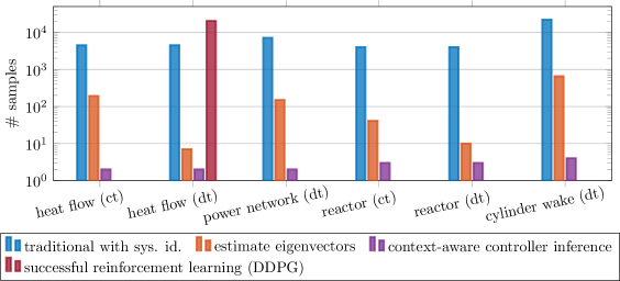
Figure 1: Summary of numerical experiments: The proposed context-aware controller inference approach provides stabilizing controllers in all experiments with an at least one order of magnitude lower number of data samples (state observations + gradient samples) than traditional two-step approaches that first identify models and then construct controllers. Reinforcement learning via deep deterministic policy gradient (DDPG) manages to stabilize only one system in our experiments, for which it requires $2\,260$ times as many samples as the proposed context-aware controller inference.

Figure 1 provides an overview about the performance of context-aware controller inference in the following numerical experiments. In all experiments, context-aware controller inference requires at least one order of magnitude fewer data samples to derive stabilizing controllers than required to learn a model for the traditional two-step data-driven control approach, including the number of gradient samples to estimate the bases of unstable dynamics. For the identification of a model that is guaranteed to capture the system dynamics for the construction of controllers in general, at least $T=N+p$ samples are necessary, where $N$ is the dimension of the full state space and $p$ the number of inputs [57]. Under certain assumptions one can identify systems with fewer samples if structure in the system dynamics is present; however, structure such as low rankness depends on the underlying physics and typically still requires subspaces of higher dimensions than the subspaces of unstable dynamics that are used in our approach; see the introduction in Section 1.

5.1.2 Comparison with reinforcement learning with deep deterministic policy gradient

We compare our approach in the discrete-time case with controllers obtained from reinforcement learning via the deep deterministic policy gradient (DDPG) method [48, 27], which can handle continuous observation and action spaces. The setup for the DDPG agents is the same as for all numerical examples up to tolerances as tuning parameters. The actor is a shallow network with a single layer and zero bias such that the resulting weight matrix corresponds to the control matrix $K\in\mathbb{R}^{p\times N}$ and can be implemented the same way for simulations as the controller designed by our proposed method. The critic takes the concatenation of state observations and the control inputs and applies to it a quadratic activation function. The result is then compressed via a fully connected layer into the Q-value. The reward function is

$$r(t,x)=\begin{cases}-\alpha\frac{x^{\mkern-1.5mu\mathsf{T}}x}{\lambda_{\mathrm{d}}n_{\mathrm{s}}(t)},&\text{if}\leavevmode\nobreak\ \lVert x\rVert_{2}>\lambda_{\mathrm{u}}\sqrt{N},\\ \alpha\left(x^{\mkern-1.5mu\mathsf{T}}x\right)n_{\mathrm{s}}(t),&\text{if controller is stabilizing},\\ -x^{\mkern-1.5mu\mathsf{T}}x,&\text{otherwise},\end{cases}$$ (31)

with the sum of steps $n_{\mathrm{s}}(t)=0.5t(t+1)$ and problem-dependent regularization parameters $\alpha=100\sqrt{N}$, $\lambda_{\mathrm{d}}$ and $\lambda_{\mathrm{u}}$. The reward function Eq. 31 is motivated by the linear-quadratic regulator design [49] to penalize the deviation of the current state from $0$; see, for example, [39] where a similar but continuous reward function has been used. The first branch in Eq. 31 evaluates to a large negative reward if the norm of the state becomes too large, which is an indication for destabilization, after which the current training episode is terminated. This is necessary to cope with the limits of numerical accuracy during the training. The second branch in Eq. 31 gives a positive reward to end the training with a stabilizing controller. Note that it is not possible to check if a given controller stabilizes the underlying system without system identification; cf. [54, 57]. We therefore fall back to a heuristic and check if the states of three consecutive time steps are close to $0$ and then return a positive reward that outweighs the previously accumulated negative rewards to end the training. The training itself is performed using discrete-time simulations of the linear models over the same time period as considered for the test simulations and starting at normally distributed, scaled random initial conditions. We have set a maximum of $1\,000$ training episodes. More details about the setup can be found in the supplementary material [56].

5.2 Experiments with linear systems

In this section, we consider two examples with linear dynamics such that no additional linearization or data shift in the sense of Eqs. 20 and 21 is necessary.

5.2.1 Disturbed heat flow

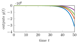
(a) CT: no controller.

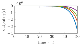
(b) DT: no controller.

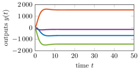
(c) CT: context-aware controller.

(d) DT: context-aware controller.

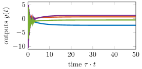
(e) DT: reinforcement learning controller.

Figure 2: Heat flow: The proposed context-aware controller inference stabilizes the system in continuous and discrete time. By using $2\,260\times$ more samples than context-aware controller inference, DDPG (reinforcement learning) also stabilizes the system, but it is more aggressive and leads to high-frequency oscillations at the beginning of the time interval.

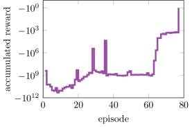
(a) DDPG training performance.

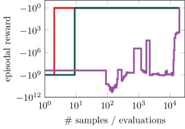
(b) Reward comparison.

Figure 3: Heat flow: DDPG takes $77$ episodes to learn a controller that satisfies the stabilization test. This corresponds to $10^{4}\times$ more state observations than context-aware controller inference if an estimate of the basis of the unstable dynamics is available a priori and $2\,260\times$ more observations if a basis has to be estimated.

Consider a two-dimensional heat flow describing the heating process in a rectangular domain affected by disturbances. We use model HF2D5 introduced in [25] to describe the underlying system. The model is continuous in time with $N=4\,489$ states and $p=2$ inputs. A discrete-time version of the model is obtained with the implicit Euler discretization with sampling time $\tau=0.1$. Both, the continuous- and discrete-time models have a single unstable eigenvalue, $r=1$, which excites the unstable system dynamics. To learn a basis of the unstable dynamics, we use $7$ gradient samples in the discrete-time case. For the continuous-time system, we use the approach described in Section 4.1 with a shift in the right open half-plane and GMRES for solving Eq. 28 without a preconditioner. We need $192$ samples of the gradient to estimate the left eigenbasis. Due to the homogeneous initial conditions, context-aware controller inference (Algorithm 1) needs $T=r+1=2$ samples to derive a controller.

Four output measurements of the system are shown in Figure 2. Context-aware controller inference smoothly stabilize the dynamics in the discrete- and continuous-time case. As comparison, we train a controller via reinforcement learning using DDPG for the discrete-time case. The training performance is shown in Figure 3(a). Reinforcement learning needs $20\,365$ state observations in $77$ episodes to learn a controller that satisfies the stabilization test. Note that the implemented test does not yield a guarantee for the constructed controller to be stabilizing, which is in contrast to our proposed method that yields a stabilization guarantee. The number of state observations needed by DDPG is nearly $5$ times the state-space dimension of the model of the system as well as $2\,260$ times the number of observations needed by context-aware controller inference, including the estimation of the eigenbasis. This can be seen in Figure 3(b) that shows the reward Eq. 31 of context-aware controller. The DDPG-learned controller also stabilizes the test simulation as shown in Figure 2(e). The two inferred controllers provide very similar closed-loop simulation behaviors in Figures 2(c) and 2(d) due to the stabilization of single real unstable eigenvalues while preserving the purely real eigenvalue structure of the problem. On the other hand, the DDPG-learned controller acts on the full spectrum and introduces complex conjugate eigenvalues that dominate the dynamics leading to an oscillatory behavior before converging to its long term steady state behavior. The DDPG controller performs also more aggressively than the inferred ones resulting in overshooting of the trajectories when compared to the steady state.

5.2.2 Brazilian interconnected power system

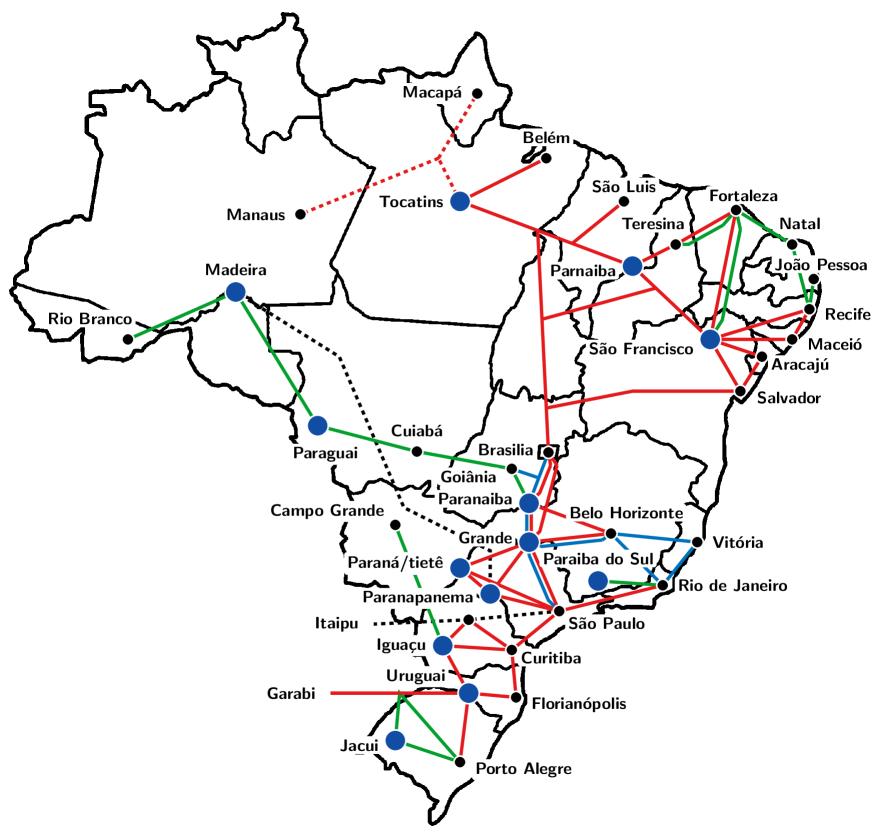
(a) Sketch of the Brazilian interconnected power system [16, 28].

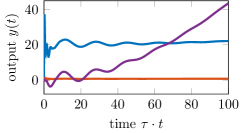
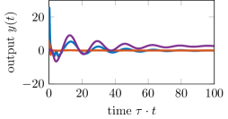
(b) DT: no controller.

(c) DT: context-aware controller.

Figure 4: Power system: The growth of output $y_{3}$ indicates an instability of the system. The proposed context-aware controller inference approach stabilizes the system leading to convergence of $y_{3}$ to 0. Only two state observations are necessary to infer a controller if a basis of the unstable dynamics is available.

(a) DDPG training performance.

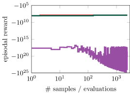
(b) Reward comparison.

Figure 5: Power system: Reinforcement learning with DDPG runs for $1\,000$ episodes but in each episode at most five time steps can be taken before the system dynamics become too unstable and lead to numerical issues, which ultimately means that no stabilizing controller is found with DDPG. In contrast, context-aware controller inference stabilizes the system after only two state observations if an estimate of a basis of the unstable dynamics is given and $152$ samples if additionally the basis has to be estimated.

We now consider a system that describes the Brazilian interconnected power system under heavy load condition. A sketch is shown in Figure 4(a). The network consists of generators and power plants, consumer clusters and industrial loads, and transmission lines, and its internal energy is controlled by reference voltage excitation; see, e.g., [28, 14]. Instabilities in the system occur by deviations from the considered heavy load condition, e.g., by disturbances, and result in an increase of the internal network energy, leading to shorts and blackouts. We consider here the bips98_606 example from [10]. The model has $N=7\,135$ states, described by ordinary differential equations and algebraic constraints, and $p=4$ inputs. Due to the algebraic constraints, we only consider the discrete-time case, which is obtained with implicit Euler and sampling time $\tau=0.1$. The model has $r=1$ unstable eigenvalues, for which we learn the corresponding left eigenvector as basis of the unstable dynamics from $150$ gradient samples.

Trajectories of three output measurements up to time $100$ are shown in Figure 4(b). The first two outputs represent the voltage at two locations in the network. Those two outputs do not yet indicate an instability. However, the average of the total network energy, which is given by the third output, increases rapidly over time in Figure 4(b) and so indicates the accumulation of internal energy. From only $T=2$ data samples of the system, we construct a stabilizing controller via context-aware inference. Outputs of the system with the inferred controller are shown in Figure 4(b) and demonstrate that the controlled system dampens the internal energy (output $y_{3}$).

We also attempted to stabilize the system with DDPG. However, even after manual parameter tuning and $1\,000$ episodes, we only obtained controllers that destabilized the system. The destabilization with DDPG happened so quickly that typically only $2$–$5$ time steps per episode were sampled, which shows that sampling data of unstable systems is challenging because after only a short time the instability leads to uninformative data collection. The training performance of DDPG is compared to controller inference in Figure 5.

5.3 Experiments with nonlinear system dynamics

5.3.1 Tubular reactor

Figure 6: Tubular reactor: Schematic representation of a tubular reactor. Reactants are injected, react inside the reactor, and the products are returned. The control goal is dampening temperature oscillations during the reaction.

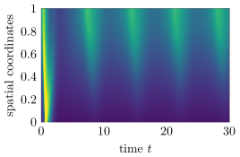
(a) CT: no controller.

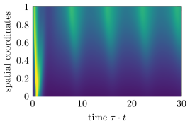
(b) DT: no controller.

(c) CT: context aware, data from linearized system.

(d) DT: context aware, data from linearized system.

(e) CT: context aware, data from nonlinear system.

(f) DT: context aware, data from nonlinear system.

Figure 7: Tubular reactor: The proposed context-aware controller inference stabilizes the system already after observing one order of magnitude fewer states than necessary for stabilizing via the traditional two-step approach. Plots (e) and (f) indicate that the proposed approach also works well on data directly obtained from the nonlinear systems.

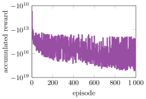
(a) DDPG training performance.

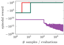
(b) Reward comparison.

Figure 8: Tubular reactor: Reinforcement learning with DDPG fails to find a stabilizing controller after $1\,000$ episodes in this example. The context-aware approach needs around $260\times$ fewer samples than what DDPG uses in $1\,000$ episodes.

We consider a tubular reactor as shown in Figure 6 and described in [23, 58]. The reaction is given by an Arrhenius term that relates temperature and specimen concentration to describe a single exothermic reaction [22]. The nonlinear model is a one-dimensional discretization of the reaction equations for Figure 6 with $N=3\,998$ states and $p=2$ control inputs. The inputs influence the temperature and specimen concentration at the left end of the tube. Additionally to the continuous-time model, we consider a discrete-time version obtained using implicit Euler for the linear part and explicit Euler for the nonlinear part with the sampling time $\tau=0.01$. We note that our approach is applicable with other time-discretization schemes as well.

Simulations without a controller showing the unstable behavior for the first half of the states representing temperature are given in Figures 7(a) and 7(b). The models have $r=2$ unstable eigenvalues, for which we need $41$ and $10$ gradient samples to estimate a basis of the unstable dynamics in the continuous and discrete time case, respectively. The observations in the continuous-time case include the use of GMRES to solve the occurring shifted systems of linear equations during the eigenvalue computations. Inspired by the reaction-diffusion nature of the problem, we use a shifted matrix resulting from the discretization of a linear diffusion equation as preconditioner. In many cases, with knowledge about the underlying application, preconditioners can be designed without system identification [34].

With the learned bases of the unstable dynamics, we use in continuous and discrete time $T=r+1=3$ data samples to design stabilizing controllers. Figures 7(c) and 7(d) show the simulations with controllers inferred from data of the models of the linearized systems (“idealized data”). In contrast, Figures 7(e) and 7(f) show the results obtained with controllers inferred from data of the original, nonlinear systems, which are sampled close to the steady state of interest.

We also trained a DDPG agent to stabilize the discrete-time system based on evaluations of the corresponding linear models. Even after $1\,000$ episodes, the training did not result in a controller that satisfied the stabilization criterion. The training results are shown in Figure 8(a). In fact, the constructed DDPG controllers often destabilize the system in the sense of Eq. 31 after 3–4 time steps. In Figure 8(b), we compare the two types of constructed controllers in terms of their rewards per data samples. The controller constructed with the proposed method stabilizes the system with fewer samples than what DDPG requires in the first training episode alone.

5.3.2 Laminar flow with an obstacle

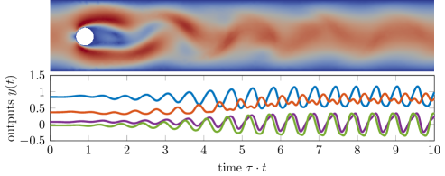
(a) DT: no controller.

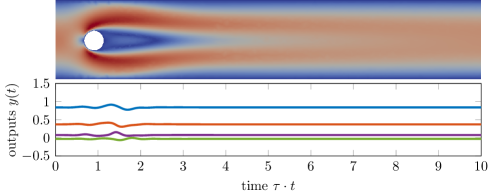
(b) DT: context-aware controller obtained from data of the linearized system.

(c) DT: context-aware controller obtained from data of the nonlinear system.

Figure 9: Flow behind a cylinder: The proposed context-aware controller inference stabilizes the system with state observations obtained from the linearized and nonlinear systems. The outputs near the disturbance initiating the unstable behavior are less oscillatory in the case of using data from the nonlinear system in this experiment.

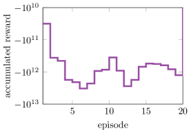
(a) DDPG training performance.

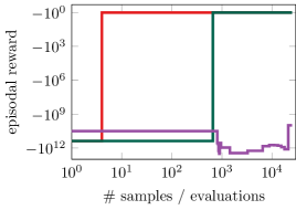
(b) Reward comparison.

Figure 10: Flow behind a cylinder: We restrict the reinforcement learning to only $20$ training episodes because obtaining samples from the linearized model is computationally expensive. The proposed approach requires around $38\times$ fewer data samples than needed in the very first DDPG episode to estimate a basis of the unstable dynamics and to infer a stabilizing controller in this example.

We consider a laminar flow behind an obstacle. The flow changes from its smooth steady state to vortex shedding under arbitrarily small disturbances. Snapshots of the flow velocity at end time are shown in Figure 9. The flow dynamics are described by the Navier-Stokes equations. The model we consider is a system of differential-algebraic equations with $N=22\,060$ states and $p=6$ control inputs, which allow to change the flow velocities in a small region right behind the obstacle. The matrices of the continuous-time model can be obtained from [3]. Due to the presence of algebraic constraints in the model, we only consider the discrete-time case, for which we obtain data with implicit Euler for the linear terms and explicit Euler for the quadratic terms with sampling time $\tau=0.0025$. The model has $r=2$ excitable unstable eigenvalues.

We need $655$ observations of the gradient to learn a basis of the unstable dynamics. Once a basis is obtained, we need $T=r+2=4$ state observations to learn a stabilizing controller with the proposed approach. Figures 9(b) and 9(c) show the simulations using controllers based on data from the linearized system and the nonlinear system, respectively. In both cases, the flow is smoothly stabilized towards the steady state.

For the DDPG agent, we stopped its training after only $20$ episodes due to high computational costs resulting from the expensive evaluation of the linear model. However, $20$ episodes are enough to demonstrate the superiority of the proposed method in terms of data requirements as shown in Figure 10. The final DDPG-controller is not stabilizing the system.

6 Conclusions

Building on the concept of context-aware learning [35, 57, 1], we have shown that for the task of finding a stabilizing controller, it is sufficient to learn only the unstable dynamics of systems, in contrast to learning models of the complete—stable and unstable—dynamics. By combining the task of stabilization with learning system dynamics in a context-aware fashion, we showed that there exist $r$ states that are sufficient to be observed for finding a guaranteed stabilizing controller, where $r$ is the dimension of the space that spans the unstable dynamics. The dimension $r$ is typically orders of magnitude lower than the dimension of the state space of all dynamics. These findings are leveraged by the proposed computational procedure that estimates bases of spaces of unstable dynamics via samples from gradients and that constructs stabilizing controllers from up to $2\,000\times$ fewer state observations than traditional data-driven control methods and variants of reinforcement learning. This enables data-driven stabilization in applications with scarce data, such as near rare events and when data generation is expensive. In contrast to the reinforcement learning method used in the numerical comparisons in this work, the proposed context-aware learning method certifies the stabilization of the underlying system by the developed theory such that the proposed context-aware controller inference provides trust for making high-consequence decisions. There are several avenues for future research. One of them is combining context-aware learning with methods for constructing manifolds of unstable dynamics [24, 59]. Working with manifolds, instead of spaces, can potentially be beneficial when systems are strongly nonlinear. At the same time, the nonlinear approximations introduced by manifolds can be computationally challenging, especially for systems with high-dimensional state spaces.

References

- [1] T. Alsup and B. Peherstorfer. Context-aware surrogate modeling for balancing approximation and sampling costs in multi-fidelity importance sampling and Bayesian inverse problems. e-print 2010.11708, arXiv, 2020. Numerical Analysis (math.NA), accepted for publication in SIAM-ASA J. Uncertain. Quantif. doi:10.48550/arXiv.2010.11708.
- [2] A. C. Antoulas, I. V. Gosea, and A. C. Ionita. Model reduction of bilinear systems in the Loewner framework. SIAM J. Sci. Comput., 38(5):B889–B916, 2016. doi:10.1137/15M1041432.
- [3] M. Behr, P. Benner, and J. Heiland. Example setups of Navier-Stokes equations with control and observation: Spatial discretization and representation via linear-quadratic matrix coefficients. e-print arXiv:1707.08711, arXiv, 2017. Mathematical Software (cs.MS). doi:10.48550/arXiv.1707.08711.
- [4] P. Benner, M. Castillo, and E. S. Quintana-Ortí. Partial stabilization of large-scale discrete-time linear control systems. In T. M. Pinkston, editor, Proceedings International Conference on Parallel Processing Workshops, 3-7 September 2001, Valencia, Spain, pages 93–98, 2001. doi:10.1109/ICPPW.2001.951856.
- [5] P. Benner, M. Castillo, E. S. Quintana-Ortí, and V. Hernández. Parallel partial stabilizing algorithms for large linear control systems. J. Supercomput., 15(2):193–206, 2000. doi:10.1023/A:1008108004247.
- [6] J. Bradbury, R. Frostig, P. Hawkins, M. J. Johnson, C. Leary, D. Maclaurin, G. Necula, A. Paszke, J. VanderPlas, S. Wanderman-Milne, and Q. Zhang. JAX: composable transformations of Python+NumPy programs (version 0.3.13), May 2022. URL: https://github.com/google/jax.
- [7] S. L. Brunton and J. N. Kutz. Data-Driven Science and Engineering: Machine Learning, Dynamical Systems, and Control. Cambridge University Press, Cambridge, 2019. doi:10.1017/9781108380690.
- [8] S. L. Brunton, J. L. Proctor, and J. N. Kutz. Discovering governing equations from data by sparse identification of nonlinear dynamical systems. Proc. Natl. Acad. Sci. U. S. A., 113(15):3932–3937, 2016. doi:10.1073/pnas.1517384113.
- [9] M. C. Campi, A. Lecchini, and S. M. Savaresi. Virtual reference feedback tuning: a direct method for the design of feedback controllers. Automatica J. IFAC, 38(8):1337–1346, 2002. doi:10.1016/S0005-1098(02)00032-8.
- [10] Cepel. Power system examples. hosted at MORwiki – Model Order Reduction Wiki, 2008. URL: http://modelreduction.org/index.php/Power_system_examples.
- [11] C. De Persis and P. Tesi. Formulas for data-driven control: Stabilization, optimality, and robustness. IEEE Trans. Autom. Control, 65(3):909–924, 2020. doi:10.1109/TAC.2019.2959924.
- [12] P. E. Farrell, D. A. Ham, S. W. Funke, and M. E. Rognes. Automated derivation of the adjoint of high-level transient finite element programs. SIAM J. Sci. Comput., 35(4):C369–C393, 2013. doi:10.1137/120873558.
- [13] M. Fliess and C. Join. Model-free control. Int. J. Control, 86(12):2228–2252, 2013. doi:10.1080/00207179.2013.810345.
- [14] F. Freitas, J. Rommes, and N. Martins. Gramian-based reduction method applied to large sparse power system descriptor models. IEEE Trans. Power Syst., 23(3):1258–1270, 2008. doi:10.1109/TPWRS.2008.926693.
- [15] R. Frostig, M. J. Johnson, and C. Leary. Compiling machine learning programs via high-level tracing. In Machine Learning and Systems (MLSys’18), 2018. URL: https://mlsys.org/Conferences/doc/2018/146.pdf.
- [16] GENI. Global Energy Network Institute – Linking renewable energy resources around the world. http://www.geni.org/, 2017. (last accessed on April 21, 2022).
- [17] G. H. Golub and C. F. Van Loan. Matrix Computations. Johns Hopkins Studies in the Mathematical Sciences. Johns Hopkins University Press, Baltimore, fourth edition, 2013.
- [18] I. V. Gosea and A. C. Antoulas. Data-driven model order reduction of quadratic-bilinear systems. Numer. Linear Algebra Appl., 25(6):e2200, 2018. doi:10.1002/nla.2200.
- [19] M. C. Grant and S. P. Boyd. Graph implementations for nonsmooth convex programs. In V. D. Blondel, S. P. Boyd, and H. Kimura, editors, Recent Advances in Learning and Control, volume 371 of Lect. Notes Control Inf. Sci., pages 95–110. Springer, London, 2008. doi:10.1007/978-1-84800-155-8_7.
- [20] M. C. Grant and S. P. Boyd. CVX: Matlab software for disciplined convex programming, version 2.2. http://cvxr.com/cvx, January 2020.
- [21] C. He and V. Mehrmann. Stabilization of large linear systems. In L. Kulhavá, M. Kárný, and K. Warwick, editors, Proceedings of the European IEEE Workshop CMP’94, Prague, September 1994, pages 91–100, 1994.
- [22] R. F. Heinemann and A. B. Poore. Multiplicity, stability, and oscillatory dynamics of the tubular reactor. Chem. Eng. Sci., 36(9):1411–1419, 1981. doi:10.1016/0009-2509(81)80175-3.
- [23] B. Kramer and K. E. Willcox. Nonlinear model order reduction via lifting transformations and proper orthogonal decomposition. AIAA J., 57(6):2297–2307, 2019. doi:10.2514/1.J057791.
- [24] B. Krauskopf, H. M. Osinga, E. J. Doedel, M. E. Henderson, J. Guckenheimer, A. Vladimirsky, M. Dellnitz, and O. Junge. A survey of methods for computing (un)stable manifolds of vector fields. Int. J. Bifurc. Chaos Appl. Sci. Eng., 15(3):763–791, 2005. doi:10.1142/S0218127405012533.
- [25] F. Leibfritz. : COnstrained Matrix-optimization Problem library – a collection of test examples for nonlinear semidefinite programs, control system design and related problems. Tech.-report, University of Trier, 2004. URL: http://www.friedemann-leibfritz.de/COMPlib_Data/COMPlib_Main_Paper.pdf.
- [26] O. Lequin, M. Gevers, M. Mossberg, E. Bosmans, and L. Triest. Iterative feedback tuning of PID parameters: comparison with classical tuning rules. Control Eng. Pract., 11(9):1023–1033, 2003. doi:10.1016/S0967-0661(02)00303-9.
- [27] T. P. Lillicrap, J. J. Hunt, A. Pritzel, N. Heess, T. Erez, Y. Tassa, D. Silver, and D. Wierstra. Continuous control with deep reinforcement learning. e-print 1509.02971, arXiv, 2015. Machine Learning (cs.LG). doi:10.48550/arXiv.1509.02971.
- [28] L. Losekann, G. A. Marrero, F. J. Ramos-Real, and E. L. F. De Almeida. Efficient power generating portfolio in Brazil: Conciliating cost, emissions and risk. Energy Policy, 62:301–314, 2013. doi:10.1016/j.enpol.2013.07.049.
- [29] A. J. Mayo and A. C. Antoulas. A framework for the solution of the generalized realization problem. Linear Algebra Appl., 425(2–3):634–662, 2007. Special issue in honor of P. A. Fuhrmann, Edited by A. C. Antoulas, U. Helmke, J. Rosenthal, V. Vinnikov, and E. Zerz. doi:10.1016/j.laa.2007.03.008.
- [30] R. v. Mises and H. Pollaczek-Geiringer. Praktische Verfahren der Gleichungsauflösung. ZAMM Z. fur Angew. Math. Mech., 9(2):152–164, 1929. doi:10.1002/zamm.19290090206.
- [31] S. K. Mitusch, S. W. Funke, and J. S. Dokken. dolfin-adjoint 2018.1: automated adjoints for FEniCS and Firedrake. J. Open Source Softw., 4(38):1292, 2019. doi:10.21105/joss.01292.
- [32] MOSEK ApS. The MOSEK optimization toolbox for MATLAB manual. Version 9.1.9, November 2019. URL: https://docs.mosek.com/9.1/toolbox/index.html.
- [33] H. Nijmeijer and A. Van der Schaft. Nonlinear Dynamical Control Systems. Springer, New York, NY, fourth edition, 2016. doi:10.1007/978-1-4757-2101-0.
- [34] J. W. Pearson and J. Pestana. Preconditioners for Krylov subspace methods: An overview. GAMM Mitt., 43(4):e202000015, 2020. doi:10.1002/gamm.202000015.
- [35] B. Peherstorfer. Multifidelity Monte Carlo estimation with adaptive low-fidelity models. SIAM/ASA J. Uncertainty Quantification, 7(2):579–603, 2019. doi:10.1137/17M1159208.
- [36] B. Peherstorfer. Sampling low-dimensional Markovian dynamics for preasymptotically recovering reduced models from data with operator inference. SIAM J. Sci. Comput., 42(5):A3489–A3515, 2020. doi:10.1137/19M1292448.
- [37] B. Peherstorfer, S. Gugercin, and K. Willcox. Data-driven reduced model construction with time-domain Loewner models. SIAM J. Sci. Comput., 39(5):A2152–A2178, 2017. doi:10.1137/16M1094750.
- [38] B. Peherstorfer and K. Willcox. Data-driven operator inference for nonintrusive projection-based model reduction. Comput. Methods Appl. Mech. Eng., 306:196–215, 2016. doi:10.1016/j.cma.2016.03.025.
- [39] J. C. Perdomo, J. Umenberger, and M. Simchowitz. Stabilizing dynamical systems via policy gradient methods. In M. Ranzato, A. Beygelzimer, Y. Dauphin, P. S. Liang, and J. Wortman Vaughan, editors, Advances in Neural Information Processing Systems, volume 34, pages 29274–29286, 2021.
- [40] J. L. Proctor, S. L. Brunton, and J. N. Kutz. Dynamic mode decomposition with control. SIAM J. Appl. Dyn. Syst., 15(1):142–161, 2016. doi:10.1137/15M1013857.
- [41] A. Ruhe. Rational Krylov sequence methods for eigenvalue computation. Linear Algebra Appl., 58:391–405, 1984. doi:10.1016/0024-3795(84)90221-0.
- [42] Y. Saad. Projection and deflation method for partial pole assignment in linear state feedback. IEEE Trans. Autom. Control, 33(3):290–297, 1988. doi:10.1109/9.406.
- [43] M. G. Safonov and T.-C. Tsao. The unfalsified control concept: A direct path from experiment to controller. In B. .A Francis and A. R. Tannenbaum, editors, Feedback Control, Nonlinear Systems, and Complexity, volume 202 of Lect. Notes Control Inf. Sci., pages 196–214. Springer, Berlin, Heidelberg, 1995. doi:10.1007/BFb0027678.
- [44] H. Schaeffer, G. Tran, and R. Ward. Extracting sparse high-dimensional dynamics from limited data. SIAM J. Appl. Math., 78(6):3279–3295, 2018. doi:10.1137/18M116798X.
- [45] P. J. Schmid. Dynamic mode decomposition of numerical and experimental data. J. Fluid Mech., 656:5–28, 2010. doi:10.1017/S0022112010001217.
- [46] P. Schulze and B. Unger. Data-driven interpolation of dynamical systems with delay. Syst. Control Lett., 97:125–131, 2016. doi:10.1016/j.sysconle.2016.09.007.
- [47] P. Schulze, B. Unger, C. Beattie, and S. Gugercin. Data-driven structured realization. Linear Algebra Appl., 537:250–286, 2018. doi:10.1016/j.laa.2017.09.030.
- [48] D. Silver, G. Lever, N. Heess, T. Degris, D. Wierstra, and M. Riedmiller. Deterministic policy gradient algorithms. Proceedings of the 31st International Conference on Machine Learning, Beijing, China, 2014. JMLR: W&CP, 32:I–387–I–395, 2014. URL: https://hal.inria.fr/hal-00938992.
- [49] V. Sima. Algorithms for Linear-Quadratic Optimization, volume 200 of Monographs and Textbooks in Pure and Applied Mathematics. Chapman and Hall/CRC, New York, 1996. doi:10.1201/9781003067450.
- [50] G. W. Stewart. A Krylov–Schur algorithm for large eigenproblems. SIAM J. Matrix Anal. Appl., 23(3):601–614, 2001. doi:10.1137/S0895479800371529.
- [51] R. Swischuk, B. Kramer, C. Huang, and K. Willcox. Learning physics-based reduced-order models for a single-injector combustion process. AIAA J., 58(6):2658–2672, 2020. doi:10.2514/1.J058943.
- [52] J. H. Tu, C. W. Rowley, D. M. Luchtenburg, S. L. Brunton, and J. N. Kutz. On dynamic mode decomposition: Theory and applications. J. Comput. Dyn., 1(2):391–421, 2014. doi:10.3934/jcd.2014.1.391.
- [53] P. Van Overschee and B. De Moor. Subspace Identification for Linear Systems: Theory, Implementation, Applications. Springer, Boston, MA, 1996. doi:10.1007/978-1-4613-0465-4.
- [54] H. J. Van Waarde, J. Eising, H. J. Trentelman, and M. K. Camlibel. Data informativity: A new perspective on data-driven analysis and control. IEEE Trans. Autom. Control, 65(11):4753–4768, 2020. doi:10.1109/TAC.2020.2966717.
- [55] A. Varga. A Schur method for pole assignment. IEEE Trans. Autom. Control, 26(2):517–519, 1981. doi:10.1109/TAC.1981.1102605.
- [56] S. W. R. Werner. Code, data and results for numerical experiments in “Context-aware controller inference for stabilizing dynamical systems from scarce data” (version 1.1), January 2023. doi:10.5281/zenodo.7530566.
- [57] S. W .R. Werner and B. Peherstorfer. On the sample complexity of stabilizing linear dynamical systems from data. e-print 2203.00474, arXiv, 2022. Optimization and Control (math.OC), accepted for publication in Found. Comput. Math. doi:10.48550/arXiv.2203.00474.
- [58] Y. B. Zhou. Model Reduction for Nonlinear Dynamical Systems with Parametric Uncertainties. PhD thesis, Massachusetts Institute of Technology, Cambridge, Massachusetts, USA, 2012. URL: http://hdl.handle.net/1721.1/77118.
- [59] A. Ziessler, M. Dellnitz, and R. Gerlach. The numerical computation of unstable manifolds for infinite dimensional dynamical systems by embedding techniques. SIAM J. Appl. Dyn. Syst., 18(3):1265–1292, 2019. doi:10.1137/18M1204395.