In the folds of the Central Limit Theorem:
Lévy walks, large deviations and higher-order anomalous diffusion

Abstract

This article considers the statistical properties of Lévy walks possessing a regular long-term linear scaling of the mean square displacement with time, for which the conditions of the classical Central Limit Theorem apply. Notwithstanding this property, their higher-order moments display anomalous scaling properties, whenever the statistics of the transition times possesses power-law tails. This phenomenon is perfectly consistent with the classical Central Limit Theorem, as it involves the convergence properties towards the normal distribution. This phenomenon is closely related to the property that the higher order moments of normalized sums of $N$ independent random variables possessing finite variance may deviate, for $N$ tending to infinity, to those of the normal distribution. The thermodynamic implications of these results are thoroughly analyzed by motivating the concept of higher-order anomalous diffusion.

1 Introduction

The Central Limit Theorem (CLT) constitutes a highly articulated and subtle galaxy of results that originated from a simple core concept, representing a milestone of the theory of probability and statistical physics because of its general and widespread applicability. In its classical form, formulated for independent and identically distributed (iid) random variables, the basic principle can be stated as follows [1, 2]: Consider iid random variables $\{x_{h}\}_{h=1,\ldots,N}$, with zero mean and finite variance, and their normalized sum,

$$z=\frac{1}{a(N)}\sum_{h=1}^{N}x_{h}\quad,$$ (1)

where $a(N)=\sqrt{N}\,\langle x^{2}\rangle$ and $\langle\cdot\rangle$ denotes the expected value with respect to the probability density of the variables $x_{h}$. Then the probability density function of $z$, $p(z;N)$, converges in distribution to the normal distribution $g(z)=e^{-z^{2}/2}/\sqrt{2\,\pi}$ for $N\rightarrow\infty$. We refer the interested reader to [3] for a chronological overview of various approaches to derive limit theorems and convergence properties of sums of random variables. The CLT and the occurrence of normal distributions yield a paradigmatic crossroad between mathematics and physics, as formulated by M. Kac (quoting H. Poincaré), “…there must be something mysterious about the normal law, since mathematicians think it is a law of nature whereas physicists are convinced that it is a mathematical theorem” [4].

In this form, the CLT represents the probabilistic interpretation of the macroscopic properties of Brownian motion, pioneered by Einstein and Smoluchowski, providing the connection between Brownian motion and diffusive phenomena [5, 6]. If the conditions of the CLT are not met, new physics appears in connection with molecular and particle motion, usually referred to as anomalous diffusion. This is the case where the variance of the variables $x_{h}$ is unbounded [7]. In this context, limit distributions different from the Gaussian typically describe the position density functions of random walks with power law tailed distributed hopping lengths and/or transition times between two consecutive changes in the direction of motion [8, 9, 10]. This phenomenon can be mathematically interpreted by the Generalized CLT [1], involving $\alpha$-stable distributions as limit distributions. Other cases of deviation from normality involve the random sums of independent random variables [11, 12], but this case is of limited interest in the present analysis.

In this article we consider the statistical properties of random motions, possessing bounded propagation velocity and linear asymptotic scaling of the mean square displacement. Despite the fact that these processes are usually classified as regular diffusion, we show that anomalies in their statistical properties arise when higher-order moments are considered. These anomalies are in one-to-one relation to the convergence properties of the density function of sums of independent random variable towards the normal distribution. In this respect, we propose a new class to which these processes should be referred to.

Natural candidates for this analysis are represented by Lévy Walks (LWs) [13, 14]. By definition, these processes possess a bounded propagation velocity and are characterized by a prescribed probability density of the transition times $T(\tau)$ [15]. In the literature, the focus has been so far almost exclusively on the case where the second-order moment of $T(\tau)$ is unbounded. This in fact provides a classical example of violation of the assumptions underlying the CLT, thus leading to anomalous diffusion [14, 16, 15, 17, 18, 19, 20, 21]. For the resulting processes in this case, the concept of an infinite density has been introduced to describe the long-term properties of the probability density function [17, 18], and interesting connections with the deterministic Lorentz gas model have been explored [22, 23]. Alternatively, these properties can also be obtained from the big jump principle, capturing rare events beyond traditional CLTs [20].

However, LWs exhibiting a long-term scaling of the mean square displacement that is linear in time, which we call Einsteinian, have been rather overlooked. They have been discussed in only few articles (e.g., [24]), despite the fact that they are characterized by peculiar features as regards the scaling of the generalized moments. These depend generically on the convergence properties of the distribution tails. Reference [25] studies this case in connection with a two-state model of a random walk consisting of the stochastic superposition of a LW and a Brownian motion process.

The main focus of this article is to investigate the scaling properties of the moment hierarchy of Einsteinian LWs. Our first main result is to show that these processes exhibit highly anomalous features in the higher-order elements of the moment hierarchy, while still preserving the long-term linear scaling of the mean square displacement and without violating the basic conditions ensuring the application of the CLT. We discuss how this phenomenon lies in the folds of the CLT, and is associated with the large-deviation properties of the limiting probability density function in the long-time limit. To describe this phenomenology systematically, we introduce the concept of higher-order anomalous diffusion, which is our second main result. In detail, any LW for which the conditions of the CLT apply, but whose transition time distribution possesses long-term power-law tails, $T(\tau)\sim\tau^{-(\xi+1)}$ with $\xi>2$, falls in this class.

The phenomenon of higher-order anomalous diffusion involves anomalies in the spectrum of generalised moments of a random walk process $X(t)$. Given a realization $x(t)$ of this process, the generalised moments are defined as [26]

$$\langle|x(t)|^{q}\rangle\sim t^{q\,\nu(q)}\,,\qquad q\in{\mathbb{R}}^{+}\quad.$$ (2)

Based on the structure of $\nu(q)$, we can distinguish three classes of stochastic motions [26]: (i) $\nu(q)=1/2$, which is characteristic of regular diffusive processes. (ii) $\nu(q)=\nu_{0}$, where $\nu_{0}\neq 1/2$ is a constant parameter independent of the order $q$ of the generalized moment. This property characterizes the class of “weak anomalous diffusive” processes. (iii) $\nu(q)$ non-uniform, i.e., generically dependent on the exponent $q$. This property characterizes the family of “strong anomalous diffusive” processes. Strong anomalous diffusion has been found in the context of transport phenomena driven either by stochastic perturbations or by deterministic chaotic forcings [27, 28, 29, 30, 31, 32]. In full generality, systems exibiting strong anomalous diffusion properties display an almost discontinuous transition in the scaling behaviour of the exponents of their generalized moments. Namely, they satisfy the condition

$$q\,\nu(q)\sim\left\{\begin{array}[]{lll}\nu_{1}q&&\mbox{for}\;q<q_{c}\\ \nu_{2}q-k&&\mbox{for}\;q>q_{c}\end{array}\right.\quad,$$ (3)

with $\nu(2)\neq 1/2$, $\nu_{2}=1$ and constant $k$. However, to the best of our knowledge, we do not know of a diffusive dynamics for which $\nu(q)$ is a continuous and smooth function of the power law index $q$.

The occurrence of higher-order anomalies has also deep implications in the thermodynamic description of the process, and this is one of the major physical issues involved in this phenomenon. Despite the linear Einsteinian scaling, a correct hydrodynamic limit for these processes, capable of reproducing the temporal behavior of the whole moment hierarchy cannot be expressed simply by the diffusion equation.

The article is organized as follows. In Section 2 we characterize the probability density function of sums of $N$ iid variables possessing bounded variance but unbounded higher-order moments. This is achieved by connecting this problem to the large deviation properties of Einsteinian LWs. Specifically, the convergence properties of CLT even in the simplest case of iid random variables, involve a singular limit, for $N$ tending to infinity, for the expected values of unbounded functions (such as the monomials of $z$). Section 2.3 analyzes further this singular limit, by means of simple and anaytically tractable examples. Section 3 develops the statistical description of the moments starting from the hyperbolic transport equations for LW. Section 4 discusses the thermodynamic and transport implications of this result, by constructing an approximate statistical two-phase model that recovers the same scaling properties of the moment hierarchy of these LWs. We also introduce the concept of “differential moment exponent spectrum”, a tool alternative to the spectrum $\nu(q)$ defined by eq. (2), which provides a convenient way to highlight the propagation mechanisms underlying anomalous diffusion properties of LWs. We conclude in Section 5 by summarising our results and elaborating on the future perspectives.

2 Large deviation properties of regular LWs

Adopting the formulation typical of Continuous Time Random Walks, a LW can be described as a process characterized by a single velocity, $v_{0}$, attaining at each transition instant either a positive or a negative velocity direction with equal probability. The statistics of the transition time $\tau$, i.e., of the time interval between two subsequent transitions, is specified by a prescribed probability density function $T(\tau)$. If $n\in{\mathbb{N}}$ indicates the operational time, counting the number of transitions, and $x_{n}$, $t_{n}$ are the walker position and the physical time after $n$ transitions, respectively, the LW is described by the iterative stochastic algorithm

$$x_{n}=x_{n-1}+v_{0}\,r_{n}\,\tau_{n}\,,\qquad t_{n}=t_{n-1}+\tau_{n}$$ (4)

where $\{r_{n}\}_{n\in{\mathbb{N}}}$ is a family of iid random variables attaining values $\pm 1$ with equal probabilities, and $\{\tau_{n}\}_{n\in{\mathbb{N}}}$ is a sequence of iid random variables sampled from the distribution $T(\tau)$. The two sequences are independent of one another. As initial condition at time $t_{0}=0$, we set $x_{0}=0$. Without loss of generality, we also set $v_{0}=1$ a.u.

In a continuous time setting, considering the physical time $t\in{\mathbb{R}}^{+}$, and assuming inertial particle motion (i.e., straight line motion between two consecutive space-time points $(x_{n},t_{n})$, $(x_{n+1},t_{n+1})$), the particle position $x(t)$ at time $t$ can be expressed as

$$x(t)=\sum_{h=1}^{N(t)}\,r_{h}\,\tau_{h}+\,r_{N(t)}\chi_{N(t)}(t)$$ (5)

where $\chi_{N(t)}=t-\sum_{h=1}^{N(t)}\tau_{h}$, and the integer $N(t)$ is defined by the inequality $\sum_{h=1}^{N(t)}\tau_{h}<t\leq\sum_{h=1}^{N(t)+1}\tau_{h}$.

A widely used expression for a transition-time probability density function possessing power-law tails is [14]

$$T(\tau)=\frac{\xi}{\tau_{0}\,(1+\tau/\tau_{0})^{\xi+1}}\quad,$$ (6)

with constant $\xi>0$ and $\tau_{0}=1$ a.u. For this class of LWs, anomalous transport properties occur for $\xi\in(0,2)$ [15]. Indicating with $\sigma_{x}^{2}(t)=\langle x^{2}(t)\rangle$ the mean square displacement (as from eq. (5), $\langle x(t)\rangle=0$), one observes the following phenomenology: for $\xi\in(0,1)$ a ballistic scaling, $\sigma_{x}^{2}(t)\sim t^{2}$; for $\xi\in(1,2)$ superdiffusive anomalous diffusion, $\sigma_{x}^{2}(t)=\sim t^{3-\xi}$; for $\xi>2$ a regular linear scaling, $\sigma_{x}^{2}(t)\sim t$. We refer to the latter LW as Einsteinian, or regular.

For $\xi>2$ the CLT applies, so that the probability density function for the normalized variable $x/\sigma_{x}(t)$ converges in a weak sense to a normal distribution [33]. This seemingly trivial phenomenology is the reason why this case has been scarcely considered in the literature so far. In fact, even for these Einsteinian LWs, interesting and highly non trivial properties occur, owing to the power-law decay of the transition-time probability density function $T(\tau)$. More precisely, we can show the existence of anomalous deviations in the scaling of the higher-order moments for any value of $\xi>2$, without violating the assumptions of the CLT. This phenomenon has been shortly addressed in [24, 25], but its implications have not been developed in detail.

We now formulate the mathematical setting for this problem, by considering the stochastic variable defined in eq. (1). The CLT states that the probability density function $p(z;N)$ associated with $z$, (possessing zero mean and unit variance), defined as the rescaled superposition of $N$ independent random variables $x_{h}$, converges to the normalized Gaussian density $g(z)=e^{-z^{2}/2}/\sqrt{2\,\pi}$ in a distributional sense [1]. Given any smooth bounded test function $\phi(z)$, this can be written as

$$\lim_{N\rightarrow\infty}\int_{-\infty}^{\infty}\phi(z)\left[p(z;N)-g(z)\right]\,dz=0$$ (7)

If the test function is not bounded, e.g. $\phi(z)=z^{2n}$ with $n>1$, we can still obtain

$$\lim_{N\rightarrow\infty}\int_{-\infty}^{\infty}z^{2\,n}\left[p(z;N)-g(z)\right]\,dz\neq 0$$ (8)

without violating the CLT. Eq. (8), that can be rewritten as,

$$\lim_{N\rightarrow\infty}\int_{-\infty}^{\infty}z^{2\,n}\,p(z;N)\,dz\neq\int_{-\infty}^{\infty}z^{2\,n}\,\left(\lim_{N\rightarrow\infty}p(z;N)\right)\,dz$$ (9)

implies that the limit for the number $N$ of the summed random variables tending to infinity does not commute, in general, with the operation of taking the expected value of unbounded functions of $z$ with respect to the corresponding probability measure. This corresponds to the fact that the higher-order moments of $p(z;N)$ may deviate, for large $N$, from those of a normal distribution. We refer to this phenomenon as an anomalous moment scaling or higher-order anomalous diffusion. We now demonstrate that this is a generic feature of LWs ultimately associated with the transition time statistics defined by eq. (6).

The number $N$ of iid random variables corresponds in a CTRW-description to the operational time of a LW; in a continuous time setting to the physical time $t$. As such the behavior of the moment hierarchy of a LW as a function of time $t$ enables us to monitor indirectly the convergence properties of $p(z,t)$ where $z=x(t)/\langle x^{2}(t)\rangle$, and ultimately the singular limit defined by eq. (9) underlying the statistical properties of the sum $\sum_{h=1}^{N}r_{h}\,\tau_{h}$ for finite $N$. To show the existence of these anomalies, therefore, our strategy is summarised as follows: (i) First, we discuss the properties of $p(z;N)$ for finite $N$. (ii) Second, we take the moments of $z$ with respect to $p(z;N)$ and analyze their scaling behavior as $N\rightarrow\infty$. (iii) Finally, we compare the result obtained with the r.h.s. of eq. (9), which are nothing but the moments of the standard normal distribution.

2.1 Scaling analysis of the finite-$N$ distribution function $p(z;N)$.

Consider first the case of the sum of identical independent random variables $\tau_{h}$,

$$\eta_{N}=\sum_{h=1}^{N}{r_{h}}\tau_{h}\quad,$$ (10)

where $\tau_{h}$ are independent random variables distributed according to eq. (6). Consider the normalized quantity

$$z_{N}=\frac{\eta_{N}-\langle\eta_{N}\rangle}{\sqrt{\langle\eta_{N}^{2}\rangle-\langle\eta_{N}\rangle^{2}}}$$ (11)

and let the exponent $\xi$ be greater than $2$. Specifically, for $\xi\in(2,3)$ the third-order moment of $T(\tau)$ is unbounded, but the second-order moment of $\eta_{N}$ is still a linear function of $N$.

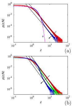
Figure 1: Probability density $p(z;N)$ vs. $z$ for the random variable $z_{N}$ defined by eq. (11) with $T(\tau)$ given by eq. (6). The arrows indicate increasing values of $N$. Solid lines represent the asymptotic scaling $P(z;N)\sim 1/z^{1+\xi}$. Panel (a): $\xi=2.9$, $N=300,\,3000$. Line (a) corresponds to the normalized Gaussian distribution $g(z)$. Panel (b): $\xi=3.5$, $N=10,\,100,\,1000$. We simulated $2\times 10^{8}$ realizations of the process in all cases, apart from the case $\xi=2.9$, $N=3000$ where we simulated $2\times 10^{7}$ realisations.

For sufficiently large $N$, the behavior of the density function $p(z;N)$ for $z_{N}$ can be approximated by

$$p(z;N)\simeq\left\{\begin{array}[]{lll}g(z)&&\mbox{for}\;|z|<z_{c}(N)\\ &&\\ \frac{C(N)}{z^{\xi+1}}&&\mbox{for}\;|z|>z_{c}(N)\end{array}\right.$$ (12)

where $z_{c}(N)\rightarrow\infty$ and $C(N)\rightarrow 0$ for $N\rightarrow\infty$, owing to the application of the CLT. This phenomenon is validated numerically in Fig. 1 for two exemplary values of $\xi$: panel (a), $\xi=2.9$; and panel (b), $\xi=3.5$.

For the class of density functions defined by eq. (6) one obtains

$$C(N)\sim N^{-(\xi-2)/2}$$ (13)

as validated numerically in Fig. 2. Observe that eq. (13) implies $C(N)\simeq C_{0}(\xi)N^{-(\xi-2)/2}$, where the prefactor $C_{0}(\xi)$ depends on $\xi$ and is an increasing function of the exponent $\xi$. This property can be justified in a rather intuitive way, by considering the limit case $N=1$ at which $p(z;1)=[T(z)+T(-z)]/2$ for $z\in{\mathbb{R}}$, where $T(z)=0$ for $z<0$, providing $p(z;1)=T(z)/2\sim\xi/2\,z^{\xi+1}$, and thus a prefactor $C_{0}(\xi)$ increasing with $\xi$. However, for $N$ sufficiently large, $C(N)|_{\xi_{1}}>C(N)|_{\xi_{2}}$, for $\xi_{1}<\xi_{2}$, where $C(N)|_{\xi}$ is the value of the prefactor for the probability density $T(\tau)$ eq. (6) characterized by the value $\xi$.

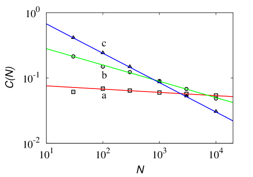
Figure 2: $C(N)$ vs. $N$ obtained for the random variable $z$ defined by eq. (11) with $T(\tau)$ given by eq. (6), rescaled statistics are depicted in Fig. 1. Symbols correspond to numerical results, lines represent eq. (13). Line (a) and ($\square$): $\xi=2.1$, line (b) and ($\circ$): $\xi=2.5$, line (c) and ($\triangle$): $\xi=2.9$.

The above results, namely eqs. (12)-(13), are consistent with the uniform and local convergence theorems that have been developed starting from the works by Berry [34] and Esseen [35], known as the Berry-Esseen theorem. Generalizations of the Berry-Esseen theorem have been thoroughly addressed in the monograph by V.V. Petrov [36] (see specifically Theorems 6 and 15 in [36]), and new estimates can be found in recent mathematical literature on the subject [37]. For the sake of precision, the existing theorems reported in [36] on local convergence apply to the case $\xi>3$. This is the reason why in Fig. 1 two cases, above and below $\xi=3$, have been reported. The above analysis indicates that it would be possible to extend these theorems also to the interval $\xi\in(2,3)$. This conjecture can be justified via a phenomenological argument (thus not a mathematical proof) developed below.

Equations (12) and (13) can be derived by applying the classical characteristic function approach to the CLT. Let $\theta_{h}=\tau_{h}-\langle\tau_{h}\rangle$ and $\phi(k)=\int_{-\infty}^{\infty}T(\theta)e^{ik\theta}d\theta$ the characteristic function of the density $T(\theta)$. Due to the power-law tail, it follows that

$$\phi(k)=1-\frac{k^{2}\,{\sigma_{\tau}}^{2}}{2}+a\,|k|^{\xi}+O(k^{\xi+\varepsilon})\quad,$$ (14)

where $\sigma_{\tau}^{2}=\langle\tau^{2}\rangle-\langle\tau\rangle^{2}$, $a$ is a constant, and $O(k^{\xi+\varepsilon})$, $\varepsilon>0$, indicates terms of higher order with respect to $|k|^{\xi}$. Since $z_{N}=\left(\sum_{h=1}^{N}\theta_{h}\right)/\sqrt{N}\sigma_{\tau}$ and the variables $\theta_{h}$ are independent, the characteristic function $\phi_{z_{N}}(k)=\left[\phi_{\theta}\left(\frac{k}{\sqrt{N}\sigma_{\tau}}\right)\right]^{N}$ is given by

$$\phi_{z_{N}}(k) = \left[1-\frac{k^{2}}{2\,N}+a\left(\frac{|k|}{\sqrt{N}\,\sigma_{\tau}}\right)^{\xi}\right]^{N}$$ (15)

$$= \left(1-\frac{k^{2}}{2\,N}\right)^{N}+N\,\frac{a}{\sigma_{\tau}^{\xi}}\frac{|k|^{\xi}}{N^{\xi/2}}\,\left(1-\frac{k^{2}}{2\,N}\right)^{N-1}+O(k^{2\xi})\quad$$

after omitting the higher-order terms. In the high $z_{N}$-limit, i.e., $\xi>2$, $k^{2}\ll 1$ and $N\gg 1$, from eq. (15) it follows that the leading terms are given by

$$\phi_{z_{N}}(k)\simeq\exp{\left(-\frac{k^{2}}{2}\right)}\left(1+\frac{a|k|^{\xi}}{\sigma_{\tau}^{\xi}N^{\xi/2-1}}\right)\quad.$$ (16)

In the limit for $N$ tending to infinity eq. (16) trivially provides the normal distribution. Conversely, for large but finite $N$ the second term within the parenthesis, corresponding to a power-law scaling of the density $p(z;N)$ as $1/z^{\xi+1}$ with a proportionality factor decaying as $N^{1-\xi/2}$, cf. to eq. (12), is responsible for the divergence of the higher-order moments. This result corresponds exactly to the singular limit expressed by eq. (9) for $N\rightarrow\infty$: The moments of the limit distribution (Gaussian) are finite and do not coincide with the limit for $N\rightarrow\infty$ of the moments of $p(z;N)$.

2.2 Scaling analysis of the higher-order moments of Einsteinian Lévy walks

Similar considerations apply for the LW eq. (5), because its kinematics is equivalent to the statistics of the sum of independent random variables (for $\xi>1$, such that $\langle\tau\rangle$ exists, and $t\simeq N\langle\tau\rangle$). This is demonstrated in Fig. 3, where we recall that $v_{0}=1$ a.u. and $x(0)=0$. In the case of the LW, the random process $X(t)$ at time $t$ is bounded by the finite propagation velocity $v_{0}$ so that $|x(t)|\leq t$. Furthermore, $t\sim N$, due to the boundedness of $\langle\tau\rangle$, implying $t\sim N\,\langle\tau\rangle$, and eqs. (12)-(13) indicate that the tails of the probability density function $p(x,t)$ scale as

$$\sigma_{x}(t)\,p(x,t)\simeq\left.\frac{\varepsilon^{*}(t)}{z^{\xi+1}}\right|_{z=x/\sigma_{x}(t)}=R(x,t)\,.\qquad\varepsilon^{*}(t)\sim t^{-(\xi-2)/2}\quad,$$ (17)

This equation is defined for $|x|\in(a^{*}(t),t)$, where $a^{*}(t)<t$, and also satisfying the condition $\lim_{t\rightarrow\infty}a^{*}(t)=\infty$, is the crossover abscissa, associated with the transition from the invariant Gaussian profile predicted by the CLT and the large-deviation property defined by eq. (17).

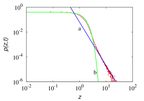
Figure 3: Probability density $p(z,t)$ vs. $z$ for $z=x(t)/\sigma_{x}(t)$ associated with a LW with $T(\tau)$ given by eq. (6) at $\xi=2.5$, $t=2000$. Symbols refer to the result of stochastic simulations using $N_{p}=2\times 10^{7}$ realizations. Line (a) is proportional to $1/z^{1+\xi}$ while line (b) represents the normalized Gaussian distribution $g(z)$.

Regarding the scaling of the even moments $\langle x^{2n}(t)\rangle$ (as for the odd moments $\langle x^{2n+1}(t)\rangle=0$), the approach used in [18] can be applied to eq. (17) leading to

$$\langle x^{2n}(t)\rangle\sim t^{\gamma_{n}}\,,\qquad\gamma_{n}=\max\{n,2\,n+1-\xi\}$$ (18)

In terms of the moment ratios (for $\xi>2$), one thus obtains

$$k_{n}(t)=\frac{\langle x^{2n}(t)\rangle}{\langle x^{2}(t)\rangle^{n}}\sim t^{\alpha_{n}}\,,\qquad\alpha_{n}=\max\{0,n+1-\xi\}\quad.$$ (19)

For $n=2$, $k_{2}(t)$ represents the kurtosis that, for an Einsteinian LW with $\xi\in(2,3)$, deviates from the value predicted by the limiting normal distribution, $k_{2}(t)=3$, as $k_{2}(t)\sim t^{3-\xi}$. This effect is a consequence of the unbounded value of the third-order moment of $T(\tau)$.

The same result can be predicted from the large-deviation properties of the distribution $p(x,t)$ for high values of $t$ starting from eq. (17). Consider the effect of the long-tail of $R(x,t)$, and set $\langle x^{2n}(t)\rangle_{R}=\sigma_{x}^{-1}(t)\int x^{2n}\,R(x,t)\,dx$. As above, consider an Einsteinian LW, i.e., $\xi>2$. Since $R(x,t)$ is symmetric and different from zero in the range $|x|\in(a^{*}(t),t)$, it follows from eq. (17) that

$$\langle x^{2n}(t)\rangle_{R} \simeq 2\,\int_{a^{*}(t)}^{t}\frac{x^{2n}}{\sigma_{x}(t)}\,R(x,t)\,dx=\frac{2\,\varepsilon^{*}(t)}{\sigma_{x}(t)}\,\int_{a^{*}(t)}^{t}x^{2n}\,[x/\sigma_{x}(t)]^{-(\xi+1)}\,dx$$ (20)

$$= 2\,\varepsilon^{*}(t)\,\sigma_{x}^{\xi}(t)\int_{a^{*}(t)}^{t}x^{2n-\xi-1}dx\quad.$$

Independently of the value of $a^{*}(t)<t$, the integral on the r.h.s. of eq. (20) scales as $\int_{a^{*}(t)}^{t}x^{2n-\xi-1}dx\sim t^{2n-\xi}$, and since $\sigma_{x}(t)\sim t^{1/2}$, one finally obtains

$$\langle x^{2n}(t)\rangle_{R}\sim t^{-(\xi-2)/2}\,t^{\xi/2}\,t^{2n-\xi}\sim t^{2n-\xi+1}\quad.$$ (21)

Since $\langle x^{2n}(t)\rangle=\langle x^{2n}(t)\rangle_{G}+\langle x^{2n}(t)\rangle_{R}$, where $\langle x^{2n}(t)\rangle_{G}$ is the contribution due to the invariant Gaussian part of the probability density,

$$\langle x^{2n}(t)\rangle_{G}=\sigma_{x}^{-1}(t)\int_{-a^{*}(t)}^{a^{*}(t)}x^{2n}g(x/\sigma_{x}(t))\,dx\sim t^{n}\quad,$$ (22)

eq. (18) follows, as the long-term moment scaling exponent, for fixed $n$, is the maximum value between $n$ and $2\,n+1-\xi$.

2.3 Examples elucidating the singular limit eq. (9).

As a first example, we consider the CTRW description of a LW parametrized with respect to the operational time $N$, i.e., $x_{N}=\sum_{h=1}^{N}r_{h}\,\tau_{h}$, in the case $\langle\tau^{2}\rangle$ is finite. Since $\langle x_{N}^{2}\rangle=N\,\langle\tau^{2}\rangle$, and

$$\langle x_{N}^{4}\rangle=N\,\langle\tau^{4}\rangle+3\,\langle\tau^{2}\rangle^{2}\,N^{2},$$ (23)

there are two cases to consider: (a) $\langle\tau^{4}\rangle<\infty$. Thus,

$$\lim_{N\rightarrow\infty}\frac{\langle x_{N}^{4}\rangle}{\langle x^{2}_{N}\rangle^{2}}=3,$$ (24)

corresponding to the kurtosis of the normal distribution. In this case, the equality is recovered in eq. (9) (at least for $n=2$). (b) $\langle\tau^{4}\rangle$ is unbounded. Consequently for any $N$

$$\langle x_{N}^{4}\rangle=\infty\,,\qquad N=1,2,\dots$$ (25)

Eq. (9) applies strictly, as $3$ is different from infinity. This clearly show in an unambiguous way the singularity of the limit underlying the CLT in the presence of power-law tailed distributions of the iid variables.

As a second example, we consider a LW in a continuous time setting. The main conceptual difference with respect to the CTRW description is that for any $t$ the moments $\langle x^{2n}(t)\rangle$ are bounded for any $t>0$ due to the finite propagation velocity. Since $v_{0}=1$ a.u., we have $\langle x^{2n}(t)\rangle\leq t^{2n}$. As regards the relation between the physical $t$ and the operational time $N$ we have

$$t=N\,\langle\tau\rangle\,\left(1+O\left(\frac{1}{\sqrt{n}}\right)\right)$$ (26)

In the present analysis the higher-order contribution $O(n^{-1/2})$ is completely irrelevant, and for the sake of notational simplicity it will be omitted. We can still apply eq. (23) but we have to consider that at time $t$ the density function for $\tau$ is not $T(\tau)$ but the censored distribution $T_{t}(\tau)$, where

$$T_{t}(\tau)=\left\{\begin{array}[]{lll}T(\tau)&&\tau<t\\ \left(1-F(t)\right)\,\delta(\tau-t)&&\tau\geq t\end{array}\right.$$ (27)

where $F(t)=\int_{0}^{t}T(\tau)\,d\tau$. Consequently, eq. (23), for a LW in a continous time frame, reads

$$\langle x^{4}(t)\rangle=\frac{t\,\langle\tau^{4}\rangle_{t}}{\langle\tau\rangle_{t}}+\frac{3\,t^{2}\,\langle\tau^{2}\rangle_{t}^{2}}{\langle\tau\rangle_{t}^{2}}=\langle x^{4}_{\rm ecc}(t)\rangle+\frac{3\,t^{2}\,\langle\tau^{2}\rangle_{t}^{2}}{\langle\tau\rangle_{t}^{2}}$$ (28)

where for any function $f(\tau)$, $\langle f(\tau)\rangle_{t}=\int_{0}^{\infty}f(\tau)\,T_{t}(\tau)$. Thus,

$$\langle x^{4}_{\rm ecc}(t)\rangle=\frac{t}{\langle\tau\rangle}\int_{0}^{\infty}\tau^{4}\,T_{t}(\tau)\,d\tau=\frac{t}{\langle\tau\rangle}\,I(t,4,\xi)+\frac{t}{\langle\tau\rangle}\frac{t^{4}}{(1+t)^{\xi}}$$ (29)

where

$$I(t,n,\xi)=\xi\int_{0}^{t}\frac{\tau^{n}\,d\tau}{(1+\tau)^{\xi+1}}=\left\{\begin{array}[]{lll}-\frac{t^{n}}{(1+t)^{\xi}}+\frac{n}{\xi-1}\,I(t,n-1,\xi-1)&&n\geq 1\\ 1-\frac{1}{(1+t)^{\xi}}&&n=0\end{array}\right.$$ (30)

It follows from eqs. (29)-(30) that

$$\langle x^{4}_{\rm ecc}(t)\rangle\sim t^{5-\xi}$$ (31)

and more generally, using the same approach,

$$\langle x^{2n}(t)\rangle\sim a\,t^{2n}+b\,t^{2n+1-\xi}$$ (32)

where $a,b>0$ are constant, consistently with the scaling theory of the probability density functions at finite $N$ developed previously.

A third analytical example, exploring the singular limit for non identically distributed random variables, is included in Appendix A.

3 Moments of LWs: hyperbolic statistical description

A convenient way for approaching the statistical characterization of LWs is to use the hyperbolic partial density formalism envisaged by Fedotov [40], applied in [41, 42] and further elaborated by Giona et al. [43]. For a LW, the partial probability densities describing the process, $p_{\alpha}(x,t;\tau)$, are parametrized with respect to the velocity direction ($\alpha=1,2$) and the transitional age $\tau\in[0,\infty)$, representing the time elapsed from the latest velocity transition. The partial densities satisfy the equations

$$\frac{\partial p_{\alpha}(x,t;\tau)}{\partial t}=-b_{\alpha}\,\frac{\partial p_{\alpha}(x,t;\tau)}{\partial x}-\frac{\partial p_{\alpha}(x,t;\tau)}{\partial\tau}-\lambda(\tau)\,p_{\alpha}(x,t;\tau)\quad.$$ (33)

Here $\lambda(\tau)$ is the transition rate, which is related to the transition time density $T(\tau)$, characterizing the CTRW formulation, by the equation

$$T(\tau)=\lambda(\tau)\,\exp\left[-\int_{0}^{\tau}\lambda(\tau^{\prime})\,d\tau^{\prime}\right]\quad.$$ (34)

In the case of eq. (6), $\lambda(\tau)=\xi/(\tau_{0}+\tau)$. In eq. (33) the velocities of the two partial waves are moving in opposite directions, i.e., $b_{1}=v_{0}=1$, $b_{2}=-v_{0}=-1$. Equations (33) are equipped with the boundary condition accounting for the velocity transitions

$$p_{\alpha}(x,t;0)=\frac{1}{2}\sum_{\beta=1}^{2}\int_{0}^{\infty}\lambda(\tau)\,p_{\beta}(x,t;\tau)\ d\tau\quad.$$ (35)

The overall probability density function for the position of a Lévy walker at time $t$ is thus $p(x,t)=\sum_{\alpha=1}^{2}\int_{0}^{\infty}p_{\alpha}(x,t;\tau)\,d\tau$. From eqs. (33) and (35), the equations for the partial moment hierarchy $m_{\alpha}^{(n)}(t,\tau)=\int_{-\infty}^{\infty}x^{n}\,p_{\alpha}(x,t;\tau)\,dx$, $n=0,1,2,\dots$, follow as

$$\frac{\partial m_{\alpha}^{(n)}(t,\tau)}{\partial t}=-\frac{\partial m_{\alpha}^{(n)}(t,\tau)}{\partial\tau}+n\,b_{\alpha}\,m_{\alpha}^{(n-1)}(t,\tau)-\lambda(\tau)\,m_{\alpha}^{(n)}(t,\tau)$$ (36)

with

$$m_{\alpha}^{(n)}(t,0)=\frac{1}{2}\sum_{\beta=1}^{2}\int_{0}^{\infty}\lambda(\tau)\,m_{\beta}^{(n)}(t,\tau)\,d\tau\quad,$$ (37)

and the overall $n$-th order moment is expressed by

$$M^{(n)}(t)=\sum_{\alpha=1}^{2}\int_{0}^{\infty}m_{\alpha}^{(n)}(t,\tau)\,d\tau\quad.$$ (38)

If initially all the particles are located at the origin, $x=0$, possess a transitional age $\tau=0$ (corresponding to a full “transitional synchronization” of the walkers’ ensemble), and their velocities are distributed amongst the two velocity directions in an equiprobable way, the initial conditions for the moment dynamics eqs. (36) and (37) read $m_{\alpha}^{(0)}(0,\tau)=\delta(\tau)/2$ and $m_{\alpha}^{(n)}(0,\tau)=0$ for $n=1,2,\dots$.

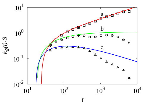
Figure 4: Deviation of the kurtosis $k_{2}(t)$ from the normal value $k_{2,{\rm norm}}=3$ vs $t$, for LWs defined by $T(\tau)$ given by eq. (6), at several values of $\xi$. Symbols represent the results of stochastic simulations using an ensemble of $N_{p}=10^{7}$ realizations, lines are the solutions of the moment equations (36)-(37). Line (a) and ($\square$): $\xi=2.5$, line (b) and ($\circ$): $\xi=3$, line (c) and ($\triangle$): $\xi=3.5$.

The moment equations (36) and (37) can be solved numerically, and their scaling in time can also be derived analytically [43], at least for the lower-order elements of the moment hierarchy. Regarding the numerics, since the “velocity of propagation through the age” is constant, $d\tau/dt=1$, a finite difference approach can be employed, setting the time step $\Delta t$ equal to the age discretization $\Delta\tau$ in order to avoid spurious effects associated with numerical diffusion. Figure 4 depicts the behaviour of the difference between the kurtosis $k_{2}(t)$ and its normal value, $k_{2,{\rm norm}}=3$, as a function of time $t$ for three different values of $\xi$ (solid lines): $\xi=2.5$, leading to an anomalous fourth-order behavior; $\xi=3$, corresponding to the threshold value between anomalous (below) and normal (above) kurtosis; and $\xi=3.5$ above the threshold. These results are obtained by solving numerically the moment equations (36) and (37),

As expected, $k_{2}(t)$ diverges to infinity at $\xi=2.5$, while for $\xi=3.5$, $k_{2}(t)-3$ relaxes asymptotically to zero. The threshold value $\xi=3$ is also interesting, as from eq. (19), $k_{2}(t)$ should at most increase with time slower than any power $t^{\eta}$, $\eta>0$. Numerical data indicates that at the threshold $\xi=3$, $k_{2}(t)$ attains, for long times, values manifestly different form $k_{2,{\rm norm}}$. In this case, whether the kurtosis would eventually converge towards a constant limit value or increase in a non-power law (possibly logarithmic) way cannot be determined from this analysis.

These predictions are further validated by numerical simulation of the stochastic dynamic (markers). The data are obtained by simulating an ensemble of $N_{p}=10^{7}$ Lévy walkers initially located at $x=0$, with $\tau=0$ and equiprobable velocity directions. The stochastic simulations qualitatively agree with the solution of the moment equations, and a consistent quantitative agreement is achieved for $t\leq 5\times 10^{2}$. As the time increases, the statistical errors associated with the finite size of the ensemble become significant. In order to reach an accurate prediction of the fourth-order moments, the size of the ensemble should be increased beyond the limit considered here, $N_{p}=10^{7}$, by several orders of magnitudes. This comparison, incidentally, shows the advantages on the use of statistical moment equations (36) for addressing the large-deviation properties of LWs with respect to the direct stochastic simulation of the dynamics.

5 depicts a simulation for long times of the scaling of the kurtosis $k_{2}(t)$ at $\xi=2.5$, from which it is possible to estimate the scaling exponent. Numerical simulation based on the moment equations provide a confirmation of the theoretical scaling $k_{2}(t)\sim t^{1/2}$ predicted by eq. (19) at $\xi=2.5$.

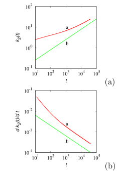
Figure 5: Kurtosis $k_{2}(t)$ vs. $t$ for a LW at $\xi=2.5$ (panel a) and its time derivative (panel (b)). Lines (a) in panels (a) and (b) represent $k_{2}(t)$ and $dk_{2}(t)/dt$, respectively, obtained from the numerical solution of the moment equations (36)-(37), lines (b) in panels (a) and (b) depict the scalings $t^{1/2}$ and $t^{-1/2}$, respectively.

4 Thermodynamic implications

Equation (18) implies interesting thermodynamic consequences for its statistical interpretion. Focusing primarily on the superdiffusive case $\xi\in(1,2)$, several authors have pointed out that the scaling relation (18) corresponds to the manifestation of strong anomalous properties [32, 18], because the family of even order moments $M^{(2n)}(t)$ does not scale with a unique exponent $\gamma_{1}$, i.e., $M^{(2n)}(t)\neq t^{n\gamma_{1}}$. This behavior indeed cannot find a statistical interpretation in terms of a single scaling function $F(z)$ for the overall density function $p(x,t)$, i.e., this distribution cannot be expressed in the form of $p(x,t)=t^{-\gamma_{1}/2}F(x/t^{\gamma_{1}/2})$ [15]. Viewed in the broader perspective of generic values $\xi>1$, thus including regular diffusive LWs, the statistical implications of Eq. (18) can be interpreted differently. While it is true that for the superdiffusive case $\xi\in(1,2)$ $\gamma_{n}\neq n\,\gamma_{1}$, Eq. (18) indicates that there exists just a single exponent branch $\gamma_{n}=2n+1-\xi$ for any $n=1,2,\dots$, at least for the even-order classical moments $M^{(2n)}(t)$. This observation will be further adressed below. Conversely, in the Einstenian case $\xi>2$, the scaling of the whole moment hierarchy derives from the combination of two different effects, thus producing the crossover behavior

$$\gamma_{n}=\left\{\begin{array}[]{lll}n&&\mbox{for}\;n<\xi-1\\ 2\,n+1-\xi&&\mbox{for}\;n>\xi-1\end{array}\right.$$ (39)

for fixed $\xi$. The lower-order elements of the moment hierarchy, up to $n<\xi-1$ are controlled by a regular diffusive scaling, while higher-order moments are subject to the same scaling that homogeneously applies to the superdiffusive case for even-order moments. In this regard, the physical phenomenology occurring for $\xi>2$, viewed in the light of the whole moment hierarchy, appears to be “more heterogeneous” than that observed for $\xi\in(1,2)$.

The physical reason for this crossover behavior can be traced back to the propagation mechanism characterizing LWs, made evident by the hyperbolic formulation. The overall dynamics of a LW is controlled by: (i) the recombination of the partial density waves associated with the two different velocity directions at finite values of the transition age $\tau$, and (ii) the existence of a statistically significant fraction of particles never performing recombination and thus propagating ballistically. The first mechanism determines the regular diffusive scaling of eq. (39) for $n<\xi-1$; the second one controls the other scaling that emerges for higher values of $n$. The latter observation becomes evident by observing that, for $n>\xi-1$, the difference $\gamma_{n+1}-\gamma_{n}=2$ is purely ballistic. The interplay between the two mechanisms is present for any value of $\xi$. While for $\xi\in(1,2)$ the ballistic propagation overwhelms the regular diffusive scaling for any even-order moments, values of $\xi>2$ permit to appreciate the simultaneous presence of the two mechanisms.

From this physical interpretation, it follows that it is almost impossible to derive a single evolution equation for the overall probability density function $p(x,t)$, which is local in time by not requiring memory integrals involving the whole previous statistical history [40], providing the correct scaling of the whole moment hierarchy, because it would involve the interplay between two completely different propagation mechanisms. Nonetheless, the analysis also suggests a different, physically simple approach towards the thermodynamics of LW processes. It consists of considering a LW ensemble as being made of two phases: a diffusionally recombining phase, and a purely ballistic one. This approach is altogether similar to the classical Landau treatment of superfluidity [44], where a viscous and a purely inviscid phase coexist. It should be mentioned that models for LWs involving fractional derivative operators have been proposed in the literature [45], describing higher-order anomalies with time-dependent exponents [46]. The resulting macroscopic properties, expressed by the scaling of the whole moment hierarchy, derive from the recombination of the two phases. If the anomalous scaling occurring for $n>\xi-1$ is the macroscopic consequence of the presence of two non-recombining ballistic waves moving in the two opposite directions, the ballistic phase can be simply described by means of two impulsive waves $P_{\pm}(x,t)$ moving at constant velocity $v_{0}$,

$$P_{\pm}(x,t)=\frac{\Phi(t)}{2}\,\delta(x\mp v_{0}\,t)\quad.$$ (40)

The key quantity here is the survival function $\Phi(t)$ [15]. At time $t=0$, $\Phi(0)=1$, and as time $t$ proceeds, particles leave the ballistic phase to join the diffusive one. The function $\Phi(t)$ does not coincide, in this approximate statistical description, to the bare survival probability $\Phi_{0}(t)=e^{-\Lambda(t)}$, where $\Lambda(t)=\int_{0}^{t}\lambda(\tau)\,d\tau$ (for $\lambda(\tau)=\xi/(1+\tau)$, $\Phi_{0}(t)=(1+t)^{-\xi}$), for the reason that a continuous flow of particles from the diffusive phase contributes to the ballistic one, and this is the reason why the ballistic moment exponent equals $\gamma_{n}=2\,n+1-\xi$, and not $2\,n-\xi$. This contribution can be modelled by considering $\Phi(t)$ to be proportional to the product of $\Phi_{0}(t)$ and of the elapsed time $t$, i.e., $\Phi(t)\sim t\,\Phi_{0}(t)$. For this reason, and in order to fulfill the initial condition, we set $\Phi(t)=(1+t)\,\Phi_{0}(t)=(1+t)^{-(\xi-1)}$, so that $\Phi(0)=1$, and $\lim_{t\rightarrow\infty}\Phi(t)=0$.

Next, we consider the diffusing phase, and let $q_{\pm}(x,t)$ be the associated partial density waves. Assuming in this approximate statistical model a constant non zero-value $\lambda_{q}>0$ for the transition rate amongst forward/backward propagating partial waves of the diffusing phase, the evolution equations for $q_{\pm}(x,t)$ coincide with those associated to a Poisson-Kac process [47, 48], onto which a continuous flux of particles from the ballistic phase is superimposed. The latter contribution can be derived from probability conservation and, assuming symmetric conditions in the recombination amongst forward and backward propagating waves, it equals $k(t)\,\left[\delta(x-v_{0}t)+\delta(x_{0}+v_{0}\,t)\right]/4$, where

$$k(t)=-\frac{d\Phi(t)}{dt}\geq 0\quad.$$ (41)

Consequently, the balance equation for $q_{\pm}(x,t)$ becomes

$$\frac{\partial q_{\pm}(x,t)}{\partial t} = \mp v_{0}\,\frac{\partial q_{\pm}(x,t)}{\partial x}\mp\lambda_{q}\,\left[q_{+}(x,t)-q_{-}(x,t)\right]$$ (42)

$$+ \frac{k(t)}{4}\,\left[\delta(x-v_{0}t)+\delta(x_{0}+v_{0}\,t)\right]$$

with the initial condition $q_{\pm}(x,0)=0$. Observe from eq. (40) the symmetry in the dynamics of the ballistic and diffusing phase, as $P_{\pm}(x,t)$ satisfy the system of equations

$$\frac{\partial P_{\pm}(x,t)}{\partial t}=\mp v_{0}\,\frac{\partial P_{\pm}(x,t)}{\partial x}-\lambda_{b}(t)\,P_{\pm}(x,t)\quad,$$ (43)

where

$$\lambda_{b}(t)=-\frac{1}{\Phi(t)}\frac{d\Phi(t)}{dt}\quad,$$ (44)

for instance $\lambda_{b}(t)=(\xi-1)/(1+t)$ for $\Phi(t)=(1+t)^{-(\xi-1)}$, equipped with the initial conditions $P_{\pm}(x,0)=\delta(x)/2$. Then eq. (42) can be rewritten as

$$\frac{\partial q_{\pm}(x,t)}{\partial t}=\mp v_{0}\,\frac{\partial q_{\pm}(x,t)}{\partial x}\mp\lambda_{q}\,\left[q_{+}(x,t)-q_{-}(x,t)\right]+\frac{\lambda_{b}(t)}{2}\left[P_{+}(x,t)+P_{-}(x,t)\right]\,.$$ (45)

Both these phases propagate ballistically, with the major difference that a continuous recombination between $q_{\pm}(x,t)$ occurs between the two partial waves of the diffusive phase, determining the long-term diffusive behavior, which is absent in the dynamics of the ballistic phase. Therefore the ballistic phase is a deterministically propagating phase without internal recombination dynamics, subject solely to a flux from and to the diffusive phase. In this sense, the analogy with the multiphase description of superfluidity is strict [44]. The system of equations (43) and (45) conserves probability,

$$\sum_{\alpha=\pm}\int_{-\infty}^{\infty}\left[q_{\alpha}(x,t)+P_{\alpha}(x,t)\right]dx=1\quad,$$ (46)

and $q_{\alpha}(x,t)\geq 0$, $P_{\alpha}(x,t)\geq 0$. Let $m_{\pm}^{(n)}(t)=\int_{-\infty}^{\infty}x^{n}\,q_{\pm}(x,t)\,dx$ be the moments associated with the diffusing phase, satisfying the balance equations

$$\frac{dm_{\pm}^{(n)}(t)}{dt}=\pm n\,v_{0}\,m_{\pm}^{(n-1)}(t)\mp\lambda_{q}\,\left[m_{+}^{(n)}(t)-m_{-}^{(n)}(t)\right]+\frac{k(t)\,(v_{0}\,t)^{n}}{4}\,\left[1-(-1)^{n}\right]\,.$$ (47)

The overall moments $M^{(n)}(t)$ of the process are the sum of the partial moments of the diffusing and ballistic phases,

$$M^{(n)}(t)=m_{+}^{(n)}(t)+m_{-}^{(n)}(t)+\frac{\Phi(t)\,(v_{o}\,t)^{n}}{2}\,\left[1+(-1)^{n}\right]\quad.$$ (48)

It follows from the symmetries that the odd moments $M^{(2n+1)}(t)=0$ are identically vanishing. Figure 6 depicts the scaling of the even moments $M^{(2n)}(t)$ for $n=1,\dots,6$ for $\xi=1.5$ (panel a) and $\xi=4.5$ (panel b), obtained from the numerical integration of the moment equations (47). Once again, we have set $v_{0}=1$ a.u., and $\lambda_{q}=1$ a.u.

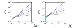
Figure 6: Scaling of the global moment hierarchy $M^{2n}(t)$ vs. $t$ obtained from the approximated “two-phase” hyperbolic model eqs. (43) and (45). Panel (a) refers to $\xi=1.5$, panel (b) to $\xi=4.5$.

The values of the long-term moment scaling exponents $\gamma_{n}$ derived from this data are depicted in Fig. 7. They perfectly agree with the theoretical result expressed by eq. (18) for $\xi>1$.

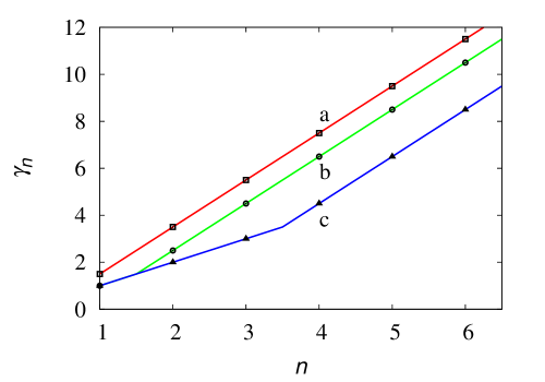
Figure 7: Moment exponents $\gamma_{n}$ vs. $n$. Lines are the theoretical predictions eq. (18), symbols the results derived from the approximate “two-phase” hyperbolic model eqs. (43) and (45). Line (a) and ($\square$) refer to $\xi=1.5$, line (b) and ($\circ$) to $\xi=2.5$, line (c) and ($\triangle$) to $\xi=4.5$.

The two-phase model eqs. (43) and (45) has been essentially derived for higher-order anomalous (superdiffusive) LWs, and the agreement between its predictions and the correct scaling of the even-order moments $M^{(2n)}(t)$ in the anomalous case, i.e., for $1<\xi<2$, is just a fortuituous case, as addressed in the next paragraph. The result for $\gamma_{n}$ can now be also recovered from the long time limit of eq. (42), which in the present case corresponds to the Kac limit (parabolic approximation) of this Poisson-Kac process: Indicating with $q(x,t)=q_{+}(x,t)+q_{-}(x,t)$ the overall density function of the diffusing phase, $q(x,t)$ satisfies in the long time limit the diffusion equation

$$\frac{\partial q(x,t)}{\partial t}=D_{q}\,\frac{\partial^{2}q(x,t)}{\partial x^{2}}+\frac{k(t)}{4}\,\left[\delta(x-v_{0}t)+\delta(x+v_{0}\,t)\right]\quad,$$ (49)

where $D_{q}=v_{0}^{2}/2\,\lambda_{q}$, from which a closed-form expression for the moment scaling exponents $\gamma_{n}$ follows that enforces the definition (41) of $k(t)$.

4.1 Generalized moments, differential moment exponents and anomalous behavior

Albeit the two phase model described in the previous paragraph correctly reproduces the scaling of the moment hierarchy $\{M^{(n)}(t)\}_{n=0}^{\infty}$ for $\xi>1$, its physical application shuold be properly limited to the case $\xi>2$, i.e., to the case of higher-order anomalous diffusion. The reason is that it predicts a Gaussian shape for the overall density function near $x=0$, and this is correct solely for $\xi>2$. Another way to look at this problem is to consider the generalized moments $\langle|x(t)|^{q}\rangle$, with $q\in{\mathbb{R}}^{+}$, that provide not only a way to detect the occurrence of strong anomalous properties, but also to probe the physical mechanism of the diffusive propagation.

In the higher-order anomalous regime $\xi>2$, the exponent spectrum $\nu(q)$ defined by eq. (2) is a non-trivial function of $q$,

$$\nu(q)=\left\{\begin{array}[]{lll}1/2&&\mbox{for}\;q<q_{c}\\ 1-(\xi-1)/q&&\mbox{for}\;q>q_{c}\end{array}\right.\quad,$$ (50)

where the crossover order $q_{c}=2\,(\xi-1)$ depends on $\xi$. This crossover is the signature of the change of regime between the two propagation mechanisms described in the previous paragraph. Let $\gamma^{*}(q)=q\,\nu(q)$, so that $\langle|x(t)|^{q}\rangle\sim t^{\gamma^{*}(q)}$. The phenomenon of higher-order anomalous behavior can be described in an even more convenient way by introducing the differential moment exponents $\nu^{*}(q)$ defined as

$$\nu^{*}(q)=\frac{d\gamma^{*}(q)}{dq}\quad.$$ (51)

The spectrum of differential exponents $\nu^{*}(q)$ is related to $\nu(q)$ by the equation $\nu^{*}(q)=\nu(q)-q\,d\nu(q)/dq$. It follows therefore that $\nu^{*}(q)$ attains two constant values independent on $q$ in the two regimes, i.e.,

$$\nu^{*}(q)=\left\{\begin{array}[]{lll}1/2&&\mbox{for}\;q<q_{c}\\ 1&&\mbox{for}\;q>q_{c}\end{array}\right.\quad,$$ (52)

thus corresponding to the diffusive and ballistic propagation mechanisms. Let us now consider the anomalous superdiffusive case, $\xi\in(1,2)$. The behavior of the moment exponents $\nu(q)$ is given by

$$\nu(q)=\left\{\begin{array}[]{lll}(3-\xi)/2&&\mbox{for}\;q<2\\ 1-(\xi-1)/q&&\mbox{for}\;q>2\end{array}\right.\quad,$$ (53)

as depicted in Fig. 8. Shown therein are results from stochastic simulations performed by considering an ensemble of $10^{6}$ particles and evaluating the long-term scaling of the generalized moments.

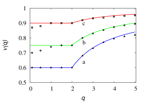
Figure 8: Moment scaling exponent $\nu(q)$ vs. $q$ for anomalous superdiffusive LWs characterized by the transition time density eq. (6) with $\tau_{0}=1$, $v_{0}=1$. Symbols are the results of stochastic simulations, lines represent eq. (53). Line (a) and ($\triangle$) refer to $\xi=1.8$, line (b) and ($\circ$) to $\xi=1.5$, line (c) and ($\square$) to $\xi=1.2$.

The slight disagreement between theory and simulations for low values of $q<1$ is due to numerical errors, in view of the relatively small size of the ensemble considered. The remarkable property associated with eq. (53) is that the crossover order $q_{c}$ does not depend on $\xi$ and is equal to $2$. This is the reason why it is not possible to detect any transition between the two propagation mechanisms from the hierarchy of integer moments $M^{(n)}(t)$, $n=0,1,2$, as $M^{(0)}(t)=1$ by probability conservation, and the first-order moment is at most constant, depending on the initial preparation of the particle system.

In terms of the differential exponents $\nu^{*}(q)$, eq. (53) yields

$$\nu^{*}(q)=\left\{\begin{array}[]{lll}(3-\xi)/2&&\mbox{for}\;q<2\\ 1&&\mbox{for}\;q>2\end{array}\right.\quad.$$ (54)

This corresponds to an effective anomalous diffusion regime characterized by the scaling law $\langle|x(t)|\rangle\sim t^{(3-\xi)/2}$, representing the lower-order part of the generalized moment hierarchy, and to a ballistic motion that becomes evident for $q>2$. The properties of the lower-order part of the generalized moment hierarchy clearly show that the approximate model developed in the previous paragraph cannot be extended beyond the range of higher-order anomalous behavior, as it predicts for the generalized moments at low $q$ values a regular diffusive scaling for any $\xi$, instead of the correct one $\langle|x(t)|^{q}\rangle\sim t^{q\,(3-\xi)/2}$.

5 Conclusions

In this article we have analyzed the statistical properties of regular Einsteinian LWs characterized by a power-law tail $T(\tau)\sim\tau^{-(1+\xi)}$, $\xi>2$, in the transition-time density function, using the CLT as a microscope to detect the peculiarities in this class of stochastic propagation processes. While the mean square displacement in the long-term limit scales linearly as a function of time, for any $\xi>2$, there exists an integer $n^{*}$ such that $M^{(2n)}(t)/t^{n}\rightarrow\infty$ for $n>n^{*}$ and $t\rightarrow\infty$. This observation has led to the concept of higher-order anomalous diffusion, and to a finer characterization of its propagation properties by considering the hierarchy of generalized moments $\langle|x(t)|^{q}\rangle$, $q\in{\mathbb{R}}^{+}$. In this perspective, any LW characterized by a power-law tail in $T(\tau)$ is intrinsically anomalous with respect to the overall statistical properties expressed by the whole moment hierarchy. For transitionally ergodic LWs ($\xi>1$) this phenomenon is essentially a consequence of two distinct transport mechanisms: (i) a diffusive scaling (be it regular for $\xi>2$, or anomalous for $1<\xi<2$) described by the scaling of the lower-order elements of the generalized moment hierarchy, and by (ii) a ballistic propagation deriving from the statistical occurrence of a significant fraction of particles never performing transitions in the velocity direction, observable for higher values of $q$. Viewed from the perspective of the properties of the moments, Einsteinian LWs possessing power-law tails in the density $T(\tau)$ as in eq. (6) provide a higher level of heterogeneity than anomalous LWs with $\xi<2$. For instance, as remarked in [24], the knowledge of the infinite density [17, 18] is not sufficient to achieve a complete prediction of the moment hierarchy, and this phenomenon has been attributed to the lack of universality of Einsteinian LWs. Regarding the latter observation, it should be noted that the qualitative behavior of $p(z;N)$ for sums of independent random variables (or of $p(x,t)$ for LWs) expressed by eqs. (12)-(13) and the corresponding scaling of the moment hierarchy is universal, in the meaning that they depend exclusively on the asymptotic scaling exponent $\xi$ controlling $T(\tau)$ and not on the fine details of this density.

The differential moment exponent spectrum $\nu^{*}(q)$ provides a convenient and clear indicator of these two concurring propagation tendencies. Starting from this compact description of the higher-order anomalies observed in LWs, a simple approximate two-phase model has been developed that correctly accounts for the scaling of the whole moment hierarchy. In principle, the same two-phase approach can be extended to anomalous diffusive LWs, i.e., in the range $1<\xi<2$, by replacing the Laplacian operator in eq. (49) with a fractional-order differential operator. This extension is left for further investigation.

As a final comment, the analogy between CLT and Renormalization Group Theory envisaged by Jona-Lasinio in 1975 [38] suggests that the results of the present manuscript as regards higher-order anomalies could be usefully transferred also to the analysis of renormalization methods in quantum field theory.

Appendix A Further example elucidating the singular limit eq. (9)

We consider the CTRW model of a Lévy walk, i.e. $x_{N}=\sum_{h=1}^{N}r_{h}\,\tau_{h}$, in the case $\tau_{h}$ are independent of one another (and of the binary variables $r_{h}$), but are not identically distributed. Each $\tau_{h}$ is characterized by a density $T_{h}(\tau)=\xi_{h}/(1+\tau)^{\xi_{h}+1}$, with $\xi_{h}$ depending on $h$. Since the variables $\tau_{h}$ are assumed to possess bounded variances, the classical CLT theorem can be easily extended [1]. In the language of LW this corresponds to a form of aging, in which the statistical properties of the transition times are functions of the operational time.

In this case, the kurtosis $\kappa_{N}$ associated with $x_{N}$ is given by

$$\kappa_{N}=\frac{\sum_{h=1}^{N}\langle\tau_{h}^{4}\rangle}{\left(\sum_{h=1}^{N}\langle\tau_{h}^{2}\rangle\right)^{2}}+3$$ (55)

where

$$\langle\tau_{h}^{2}\rangle=\frac{2}{(\xi_{h}-1)(\xi_{h}-2)}\,,\qquad\langle\tau_{h}^{4}\rangle=\frac{24}{(\xi_{h}-1)(\xi_{h}-2)(\xi_{h}-3)(\xi_{h}-4)}$$ (56)

Assume that $\langle\tau^{4}_{h}\rangle$ were bounded for any $h=1,2,\dots$, while $\lim_{h\rightarrow\infty}\langle\tau^{4}_{h}\rangle=\infty$. This corresponds to the case where $\xi_{h}>4$, and $\lim_{h\rightarrow\infty}\xi_{h}=4$. For instance, one may consider the situation described by the sequence of exponents

$$\xi_{h}=3+\frac{2}{1+h^{\beta}}$$ (57)

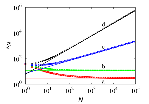
Figure 9: Kurtosis $\kappa_{N}$ vs $N$ deriving from eq. (55), with $\xi_{h}$ given by eq. (57). Symbols (a) refer to $\beta=0.5$, (b) to $\beta=1$, (c) to $\beta=1.5$, (d) to $\beta=2$. Solid line (a) corresponds to $\kappa_{n}=3$, corresponding to the Gaussian limit, line (b) to $\kappa_{n}=\mbox{const}\neq 3$, line (c) to $\kappa_{n}\sim n^{1/2}$, line (d) to $\kappa_{n}\sim n$.

Since $\sum_{h=1}^{N}\langle\tau_{h}^{2}\rangle\sim N^{2}$, and $\sum_{h=1}^{N}\langle\tau_{h}^{4}\rangle\sim\sum_{h=1}^{N}h^{\beta}\sim N^{1+\beta}$, it follows that

$$\kappa_{N}=\left\{\begin{array}[]{lll}3&&\beta<1\\ c\neq 3&&\beta=1\\ d\,N^{\beta-1}+O(N^{\beta-2})&&\beta>1\end{array}\right.$$ (58)

where $c,\,d>0$ are constant, and consequently the asymptotic behavior of the fourth-order moment depends towards the rate of convergence of $\xi_{h}$ towards the limit value $\xi=4$, determining unbounded $\langle\tau^{4}\rangle$. This phenomenon is depicted in figure 9. This simple analytical example shows the subtle role of the singular limit eq. (9) controlling the scaling of the higher-order elements of the moment hierarchy of sums of independent random variables fulfilling the hypothesis of the CLT.

References

.

References

- [1] B. V. Gnedenko and A. N. Kolmogorov, Limit distributions for sums of independent random variables (Addison-Wesley, Cambridge MA, 1954).
- [2] M. Kardar, Statistical Physics of Particles (Cambridge Univ. Press, Cambridge, 2007).
- [3] H. Fischer, A History of the Central Limit Theorem (Springer, New York, 2010).
- [4] M. Kac, Statistical Independence in Probability Analysis & Number Theory (Dover Publ. New York, 2018).
- [5] A. Einstein, Investigations on the theory of Brownian movement (Dover Publ., Mineola, 1956).
- [6] B. Cichocki (Ed.) Marian Smoluchowski - Selected Scientific Works (WUW Press, Warsaw,2017).
- [7] V. V. Uchaikin and V. M. Zolotarev, Chance and Stability: Stable Distributions and their Applications (de Gruyter, Berlin, 1999).
- [8] E. W. Montroll and G. H. Weiss, J. Math. Phys. 6, (1965) 167.
- [9] R. Metzler and J. Klafter, Phys. Rep. 339, (2000) 1.
- [10] R. Klages, G. Radons and I.M. Sokolov (Eds.), Anomalous Transport (Wiley-VCH, Weinheim, 2008).
- [11] V.M. Kruglov and V. Yu. Korolev, Prob. Theory and Math. Stat. 2, (1990) 10.
- [12] B. V. Gnedenko and V. Yu. Korolev, Random Summation (CRC Press, Boca Raton, 1996).
- [13] M. F. Shlesinger, J. Klafter and B. J. West, Physica A 140, (1986) 212.
- [14] M. F. Shlesinger, B. J. West and J. Klafter J, Phys. Rev. Lett. 58, (1987) 1100.
- [15] V. Zaburdaev, S. Denisov and J. Klafter, Rev. Mod. Phys. 87, (2015) 483.
- [16] M. Schmiedeberg, V. Yu. Zaburdaev and H. Stark, J. Stat. Mech, (2009) P12020.
- [17] A. Rebenshtok, S. Denisov, P. Hänggi and E. Barkai, Phys. Rev. Lett. 112, (2014) 110601.
- [18] A. Rebenshtok, S. Denisov, P. Hänggi and E. Barkai, Phys. Rev. E 90, (2014) 062135.
- [19] I. Fouxon, S. Denisov, V. Zaburdaev and E. Barkai, J. Phys. A 50, (2017) 154002.
- [20] A. Vezzani, E. Barkai and R. Burioni, Phys. Rev. E 100, (2019) 012108.
- [21] A. Miron, Phys. Rev. Lett. 124, (2020) 140601.
- [22] L. Zarfaty, A. Peletskyi, I. Fouxon, S. Denisov and E. Barkai, Phys. Rev. E 98, (2018) 010101(R).
- [23] I. Fouxon and P. Ditlevsen, J. Phys. A 53, (2020) 415004.
- [24] A. Rebenshtok, S. Denisov, P. Hänggi and E. Barkai, Math. Model. Nat. Phenom. 11, (1016) 76.
- [25] X. Wang, Y. Chen and W. Deng, Phys. Rev. Res. 2, (2020) 013102.
- [26] P. Castiglione, A. Mazzino, P. Muratore Ginanneschi and A. Vulpiani, Physica D 134, (1999) 75.
- [27] P. Castiglione, A. Mazzino, P. Muratore-Ginanneschi, Physica A 280, (2000) 60.
- [28] K. H. Andersen, P. Castiglioni, A. Mazzino and A. Vulpiani, Eur. Phys. J. B 18, (2000) 447.
- [29] R. Artuso and G. Cristadoro, Phys. Rev. Lett. 90, (2003) 244101.
- [30] D. P. Sanders and H. Larralde, Phys. Rev. E 73, (2006) 026205.
- [31] N. Gal and D. Weihs, Phys. Rev. E 81, (2010) 020903(R).
- [32] J. Vollmer, L. Rondoni, M. Tayyab, C. Giberti and C. Mejia-Monasterio, Phys. Rev. Res. 3, 013067 (2021).
- [33] P. Billingsley, Probability and Measure (J. Wiley & Sons, New York, 1995).
- [34] A. C. Berry, Trans. Amer. Math. Soc. 49, (1941) 122.
- [35] C.-G. Esseen, Acta Math. 77, (1945) 1.
- [36] V. V. Petrov, Sums of Independent Random Variables (Springer-Verlag, Berlin, 1975).
- [37] Yu. S. Nefedova and I. G. Shevtsova, Theor. Probab. Appl. 57, (2013) 28.
- [38] G. Jona-Lasinio, Nuovo Cimento 26, (1975) 98.
- [39] I. Calvo, J. C. Cuchi, J. G. Esteve and F. Falceto, J. Stat. Phys. 141, (2010) 409.
- [40] S. Fedotov, Phys. Rev. E 93, (2016) 020101(R).
- [41] S. Fedotov and N. Korabel, Phys. Rev. E 95, (2017) 030107(R).
- [42] H. Stage and S. Fedotov, Eur. Phys. J. B 90, (2017) 225.
- [43] M. Giona, A. Cairoli and R. Klages, Phys. Rev. X 12, (2022) 021004.
- [44] A. Schmitt Introduction to Superfluidity (Springer Int. Publ., Cham, 2015).
- [45] J. P. Taylor-King, R. Klages, S. Fedotov and R. A. Van Gorder, Phys. Rev. E 94, (2016) 012104.
- [46] M. A.F. dos Santos, F. D. Nobre and E. M. F. Curado, Commun. Nonlinear. Sci. Numer. Simulat. 92, (2021) 105490.
- [47] M. Kac, Rocky Mount. J. Math. 4, (1974) 497.
- [48] M. Giona, A. Brasiello and S. Crescitelli, J. Phys. A 50, (2017), 335002.
.