Search-based Software Testing Driven by Automatically Generated and Manually Defined Fitness Functions

Abstract.

Search-based software testing (SBST) typically relies on fitness functions to guide the search exploration toward software failures. There are two main techniques to define fitness functions: (a) automated fitness function computation from the specification of the system requirements, and (b) manual fitness function design. Both techniques have advantages. The former uses information from the system requirements to guide the search toward portions of the input domain more likely to contain failures. The latter uses the engineers’ domain knowledge.

We propose ATheNA, a novel SBST framework that combines fitness functions automatically generated from requirements specifications and those manually defined by engineers. We design and implement ATheNA-S, an instance of ATheNA that targets Simulink^® models. We evaluate ATheNA-S by considering a large set of models from different domains. Our results show that ATheNA-S generates more failure-revealing test cases than existing baseline tools and that the difference between the runtime performance of ATheNA-S and the baseline tools is not statistically significant. We also assess whether ATheNA-S could generate failure-revealing test cases when applied to two representative case studies: one from the automotive domain and one from the medical domain. Our results show that ATheNA-S successfully revealed a requirement violation in our case studies.

1. Introduction

Software failures in cyber-physical systems (CPS) can have catastrophic and costly consequences. For example, automotive software failures led to severe injuries and the loss of human lives (e.g.,  (Uber, line; GMD, line; TeslaCrash, line)). Car manufacturers had to recall their vehicles, causing reputation damage and millions of U.S. Dollars lost (e.g., (GMD, line; Honda, line; TeslaDefects, line; StellantiDefects, line; LandRover, line; Recalls, line; Recall-problem, line)). To prevent these scenarios, CPS engineers extensively test their systems to detect safety-critical software failures (Altinger et al., 2014; Garousi et al., 2018; Zhou et al., 2018; Duan et al., 2018). Automated testing tools facilitate this activity (e.g.,  (Menghi et al., 2020; Annpureddy et al., 2011; Matinnejad et al., 2015; Abdessalem et al., 2018)). These tools are regularly used in safety-critical CPS domains, including automotive (e.g., (Matinnejad et al., 2015)), aerospace (e.g., (Menghi et al., 2020)), and medical (e.g., (Majikes et al., 2013)).

Automated testing often (e.g., (Menghi et al., 2020)) relies on search-based software testing (SBST). SBST iteratively generates test cases until a software failure is detected or the SBST framework exceeds the time budget allotted for the testing activity. It relies on different (a) optimization algorithms (e.g., (Mathesen et al., 2019; Cohen and Belta, 2021)), (b) input types (e.g., (Ramezani et al., 2021)), (c) surrogate models (e.g., (Nejati et al., 2023; Menghi et al., 2020)), and (d) fitness functions (e.g., (Matinnejad et al., 2015)). This paper considers the fitness function design, a challenging task for designing effective SBST frameworks ((Salahirad et al., 2020; Wilkerson and Tauritz, 2011; Arcuri and Briand, 2011; Sahin and Akay, 2016; Bajaj and Sangwan, 2019; Aleti et al., 2017; Almulla and Gay, 2020; Sadri-Moshkenani et al., 2022)).

Fitness functions guide SBST frameworks in generating new test cases. They provide metrics (a.k.a. fitness values) that estimate how close the test cases are to detecting a failure (Harman and Clark, 2004). To effectively and efficiently generate failure-revealing test cases, it is critical to select appropriate fitness functions (Wilkerson and Tauritz, 2011; Arcuri and Briand, 2011; Sahin and Akay, 2016; Bajaj and Sangwan, 2019). Fitness landscape analysis activities evaluate how the fitness value changes over the search space and usually support the fitness function design (e.g. (Kim and Moon, 2003; Pohlheim, 1999; Aleti et al., 2017)). Fitness landscape analysis can help understand the search process and its probability of success (e.g. (Hart and Ross, 2001; Kim and Moon, 2002, 2003)). However, despite the breadth and diversity of testing domains and solutions, the design of fitness functions is still complex and time-consuming (e.g., (Salahirad et al., 2020; Almulla and Gay, 2020; Amal et al., 2014)).

There are two mainstream techniques to define fitness functions: automated generation and manual definition.

Automated generation of the fitness function (e.g., (Fainekos et al., 2019; Donzé and Maler, 2010; Varnai and Dimarogonas, 2020; Arrieta et al., 2020; Pant et al., 2017; Mehdipour et al., 2019; Lindemann and Dimarogonas, 2019)) derives the fitness function from other artifacts without any human intervention. For example, many SBST frameworks (e.g., (Annpureddy et al., 2011; Menghi et al., 2020; Waga, 2020; Ernst et al., 2021)) use fitness functions to compute the robustness values derived from temporal logic specifications expressing system requirements (e.g., (Fainekos et al., 2019; Menghi et al., 2019; Pant et al., 2017; Haghighi et al., 2019)). These functions typically use the requirement structure to guide the search toward portions of the input domain more likely to lead to system failures. Automatically generated fitness functions support SBST in the detection of failures (e.g., (Donzé and Maler, 2010; Varnai and Dimarogonas, 2020; Haghighi et al., 2019; Arrieta et al., 2020)). They were used to detect failures in industrial models (e.g., (Menghi et al., 2020; Jin et al., 2014)), and are used within international tool competitions (e.g., (Ernst et al., 2022)). Automatically generated fitness functions are general purpose and do not use engineers’ domain knowledge for the fitness value computation.

Unlike the automated approach, manual fitness function definition (e.g.,  (Abdessalem et al., 2018; Wilkerson and Tauritz, 2011; Matinnejad et al., 2016a; Ben Abdessalem et al., 2018; Matinnejad et al., 2014)) requires engineers to design the fitness functions using their experience and domain knowledge. For example, engineers can manually define fitness functions to guide the search toward the generation of inputs that are more likely to show the violation of liveness, stability, smoothness, and responsiveness requirements (Matinnejad et al., 2015). Manually defined fitness functions effectively and efficiently support SBST — they enable the detection of failures that domain experts could not find by manual testing (e.g.,  (Matinnejad et al., 2015)). Manual fitness function design enables engineers to write model-specific fitness functions that guide the search toward specific areas that are more likely to contain failures, e.g., the boundaries of the input domain. However, manually defined fitness functions are biased and, in some cases, may concentrate the search on areas of the input domains that do not contain failures.

This work proposes ATheNA (AuTomatic-maNuAl search-based testing), a novel black-box SBST framework driven by automatically generated and manually defined fitness functions. ATheNA combines the benefits of automatically generated and manually defined fitness functions: it exploits both the structure of the requirements and the engineers’ domain knowledge to guide the search toward specific areas of the input domain that are likely to reveal software failures. In addition, we define ATheNA-S, an instance of ATheNA that supports Simulink^® models. We consider Simulink^® models since they are widely used for specifying the behavior of CPSs (Boll et al., 2021; Liebel et al., 2018) in a variety of domains, including automotive (Matinnejad et al., 2015), energy (Jin et al., 2014) and medical (Sankaranarayanan and Fainekos, 2012). We implement ATheNA-S as a plugin for S-Taliro (Annpureddy et al., 2011), a well-known SBST framework for Simulink^® models recently classified as ready for industrial usage (Kapinski et al., 2016). ATheNA is the first solution that enables engineers to combine manual and automatic fitness function design. Enabling the combination of the two fitness functions is a significant contribution to the software engineering field since it allows engineers to exploit the benefits of the combined fitness function that, as we show in our evaluation, outperforms existing solutions.

We evaluate the effectiveness and efficiency of ATheNA-S in generating failure-revealing test cases. We compare ATheNA-S with S-Taliro (Annpureddy et al., 2011), a tool that supports automatically generated fitness functions, and ATheNA-SM, a customization of ATheNA-S that supports manually defined fitness functions. We consider seven models and $27$ requirements from ARCH 2021 (Ernst et al., 2022; ARCH, line), an international SBST competition for Simulink^® models held as a part of the international conference on Computer Safety, Reliability, and Security (SAFECOMP) (DBL, 2021). For each requirement, we consider a set of assumptions for the inputs of the model. In total, we compare the tools by considering $39$ assumption-requirement combinations. We considered two versions of ATheNA that use different functions to combine the manual and automatic fitness values. Our results show that (a) ATheNA-S performs better than the baseline tools for most of our assumption-requirement combinations ($\approx 74\%$ and $100\%$ for the two versions of ATheNA we considered), (b) ATheNA-S generates more failure-revealing test cases than S-Taliro (+$7.9\%$ and +$11.9\%$) and ATheNA-SM (+$8.1\%$ and +$12.1\%$), and (c) the difference between the runtime performance of ATheNA-S and the baseline tools is not statistically significant for one version of ATheNA and negligible for the other. Additionally, we assess how applicable and useful is ATheNA-S in generating failure-revealing test cases for two large Simulink^® models. The first model is an electrical automotive software control system (AUT, line) developed as a part of the EcoCAR Mobility Challenge (Eco, line), a competition sponsored by the U.S. Department of Energy (DOE, line), General Motors (GM, line), and MathWorks (Mat, line). The second model is mechanical ventilator (Miller, line) developed by MathWorks (Mat, line). We evaluate whether ATheNA-S could generate any failure-revealing test cases. Our results show that ATheNA-S could generate a failure-revealing test within practical time limits for both the automotive and the ventilator models. We present and discuss the problems identified by the failure-revealing test cases returned by ATheNA-S.

To summarize, our contributions are:

• We propose the ATheNA framework (Section 2);

• We define ATheNA-S, an instance of ATheNA that supports Simulink^® models (Section 3);

• We implement ATheNA-S as a plugin for S-Taliro (Section 4);

• We empirically assess the benefits of ATheNA (Section 5);

• We discuss the impact of our findings on the software engineering practice (Section 6).

This work is organized as follows: Section 2 presents ATheNA. Section 3 describes the instance of ATheNA that targets Simulink^® models. Section 4 provides implementation details. Section 5 empirically assesses our contribution. Section 6 discusses our findings and presents threats to validity. Section 7 presents related work. Section 8 concludes the work.

2. Automatic-Manual SBST

Figure 1 provides an overview of the ATheNA (AuTomatic-maNuAl) search-based testing framework. Squared boxes report the steps of ATheNA. Incoming and outgoing arrows describe the inputs and outputs of the different steps. Arrows with no source represent the inputs of the ATheNA framework. Arrows with no destination represent the outputs of the ATheNA framework. Arrows connecting two boxes link subsequent steps.

Figure 1. Overview of the ATheNA testing framework.

[Flowchart representing the steps of the ATheNA testing framework.]Flowchart representing the connection between the six steps of the ATheNA testing framework. The main iteration loop is formed by Steps 1, 2, and 3. Step 3 is further split into Steps 4, 5, and 6. Steps 5 and 6 are executed in parallel and feed into Step 4.

ATheNA has four inputs: a model of the system to be tested ($S$); an assumption on the system inputs ($A$), a time budget ($T$), and a requirement ($\varphi$). The output of ATheNA is a failure-revealing test case ($\texttt{tc}(\texttt{i})$) or an indication that no failure-revealing test case was found (NFF — No Failure Found) within the time budget.

To detect a failure-revealing test case, ATheNA iteratively repeats the steps presented in Figure 1:

• Input Generation ( ). It generates an input (i) for the system model ($S$) that satisfies the assumption ($A$);

• System Execution ( ). It runs the system model ($S$) with the generated input (i) and obtains a system execution ($S(\texttt{i})$).

• Fitness Assessment ( ). It computes the fitness value ($f(S(\texttt{i}))$) associated with the obtained system execution ($S(\texttt{i})$) and assesses whether the fitness value is below a threshold value.

A test case ($\texttt{tc}(\texttt{i})$) associated with the input (i) is failure-revealing if: (a) the input satisfies the assumption ($A$), i.e., $\texttt{i}\models A$, and (b) the fitness value ($f(S(\texttt{i}))$) is smaller than a threshold value (typically the value $0$). Typically, the fitness value is negative if the property is violated and positive otherwise. In addition, the higher the positive value computed by $f_{a}$, the further the system is from violating its requirement, while lower negative values indicate that the system is further from satisfying its requirement (Fainekos and Pappas, 2006; Fainekos et al., 2019; Waga, 2020; Menghi et al., 2019; Ernst et al., 2022).

The ATheNA framework terminates when a failure-revealing test case ($\texttt{tc}(\texttt{i})$) is detected or when the framework exceeds the time budget ($T$) without finding any failure-revealing test case. For the former case, ATheNA returns the failure-revealing test case. For the latter case, ATheNA returns the NFF value.

The fitness value ($f(S(\texttt{i}))$) is used to guide the ATheNA framework. The search algorithm tries to find an input associated with a negative fitness value. To reach this goal, it uses the fitness value computed in step  to drive the generation of the next input ( ).
The Input Generation, System Execution, and Fitness Assessment components are shared by many existing SBST tools, such as S-Taliro (Annpureddy et al., 2011), Breach (Donzé, 2010), FalStar (Ernst et al., 2019), FalCAuN (Waga, 2020), falsify (Yamagata et al., 2021), FalStar (Ernst et al., 2019), and ForeSee (Zhang et al., 2021).

To compute the fitness value, ATheNA combines manually defined and automatically generated fitness functions and has the following steps:

• ATheNA Fitness ( ). It returns a fitness function ($f$) that combines the values computed by the manually defined and automatically generated fitness functions. Depending on the testing necessities, the fitness function $f$ can prioritize one of the two values. The function can also change the prioritization policy dynamically during the search if the fitness value is not effectively guiding the SBST framework.

• Automatic Fitness ( ). It returns a fitness function ($f_{a}$) automatically generated from requirement $\varphi$. The requirement is automatically compiled into a function that, given a system execution $S(\texttt{i})$, computes a fitness value ($f_{a}$).

• Manual Fitness ( ). It returns a fitness function ($f_{m}$) manually defined by the engineers. It computes a fitness value for the system execution $S(\texttt{i})$.

ATheNA can be instantiated by considering different modeling formalisms. For ATheNA to be applicable for a CPS, that CPS is assumed to be a reactive system, i.e., it takes some inputs (produced by the Input Generation component) and produces some outputs that can be monitored (used by the Fitness Assessment component). Alternative instances of ATheNA differ in the implementation of the Input Generation, System Execution, Fitness Assessment, ATheNA Fitness, Automatic Fitness, and Manual Fitness components.

One instance of ATheNA that targets Simulink^® models and assumes that the inputs and the outputs of the CPS are signals over time is presented in the next section.

3. Automatic-Manual SBST for Simulink^®

This section describes ATheNA-S, an instance of ATheNA that supports Simulink^®, a graphical language for model design.

Figure 2 presents our running example: the variation of the Automatic Transmission (AT) model provided by Mathworks (ATBenchmark, line), used in the applied verification for continuous and hybrid systems competition (Ernst et al., 2022; ARCH, line).

Simulink^® provides visual constructs to design a system model ($S$). Blocks typically represent operations and constant values. They are aggregated into subsystems labeled with ports that identify the inputs and outputs of the subsystems. For example, Engine is one of the subsystems of the Simulink^® model of Figure 2. It has two input ports (Ti and Throttle) and one output port (Ne). Connections link input and output ports. For example, a connection links the output port Ne of the Engine subsystem to the input port Ne of the Transmission subsystem. The inputs and outputs of a Simulink^® model are represented by the inports and outports blocks. For example, in Figure 2, there are two inputs (Throttle, and Brake) and three outputs (Speed, RPM, and Gear).

We instantiated ATheNA to support Simulink^® models as follows:

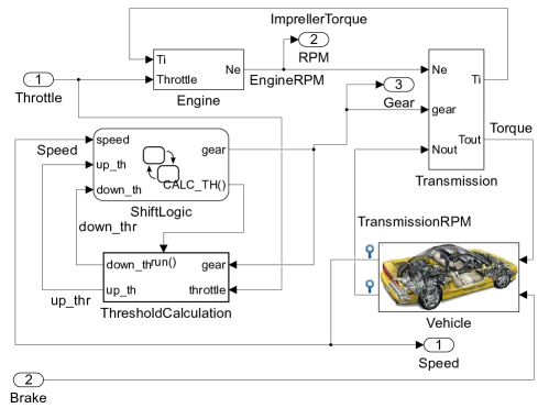
Figure 2. Simulink^® model of the AT example.

[Simulink^® model of the AT example.]Simulink^® model of the AT example. The model takes as input a Throttle and Brake signals. It returns as output a Speed, Engine RPM, and Gear signals. The model is formed by five subsystems: Engine, Transmission, Vehicle, Shift Logic and Threshold Calculation.

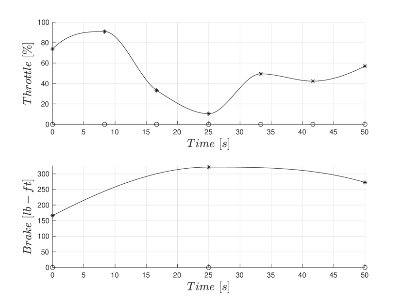
(a) Example of input signals for the AT model between $0s$ and $50s$.

[Example of Throttle and Brake signals for the AT model.]Example of Throttle and Brake continuous signals for the AT model. The Throttle signal uses seven control points. The Brake signal uses three control points.

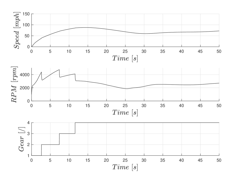
(b) Output signals for the AT model for the input of Figure 3(a).

[Example of Speed, Engine RPM, and Gear signals for the AT model.]Example of Speed, Engine RPM, and Gear signals for the AT model. The plots show the car accelerating until it reaches Gear four and then keeping a constant speed around $70mph$.

Figure 3. Example input and output for the AT Simulink^® model.

Input Generation ( ). The input generation step generates a set of signals $\texttt{i}=\{i_{1},i_{2},\ldots,i_{m}\}$ — one per inport. For example, for the AT model, ATheNA generates the input signals for the Throttle and Brake inports. A signal is a function $f:\mathbb{T}\rightarrow$, where $\mathbb{T}$ is a non-singular bounded interval $[0,b]$ of that represents the simulation time domain of system $S$. The Simulink^® simulator requires engineers to specify the input of the simulation. Figure 3(a) presents an example of an input for the AT model. The input contains the two input signals for the Throttle and Brake inports defined over the simulation time domain $[0,50]$s.

Assumption $A$ guides the generation of new input signals. For each input signal $i_{i}\in\texttt{i}$, it contains a triple $\langle int_{i},R_{i},n_{i}\rangle$ made of an interpolation function ($int_{i}$), a value range ($R_{i}$) and a number of control points ($n_{i}$). ATheNA-S generates each input signal $i_{i}$ by selecting $n_{i}$ time instants, i.e., $t_{1},t_{2},\ldots,t_{n_{i}}$, within the time domain $\mathbb{T}=[0,b]$, such that $t_{1}=0$, $t_{n_{i}}=b$ and $t_{1}<t_{2}<\ldots<t_{n_{i}}$. The values of $t_{1},t_{2},\ldots,t_{n_{i}}$ can also be chosen to ensure a fixed difference between consecutive time instants, i.e., for all $t_{j},t_{j+1}$ with $j\in\{1,2,\ldots n_{i}-1\}$, the value of $t_{j+1}-t_{j}$ is fixed. Then, ATheNA-S selects a value $i_{i}(t_{j})$ from value range $R_{i}$ for each time instant $t_{j}$. The interpolation function (e.g., piecewise constant, linear or piecewise cubic) is then used to generate the values assumed by the input signal $i_{i}$ over the rest of the time domain $\mathbb{T}$. For example, the input signals for the Throttle and Brake reported in Figure 3(a) are generated by considering the value range $[0,100]$ for the throttle percentage applied to the engine (%), and $[0,325]$ for the pound-foot (lb-ft) torque applied by the brake. To generate the input signals, the Piecewise Cubic Hermite Interpolating Polynomial (pchip) interpolation function (PCHIP, line) and $7$ and $3$ control points are respectively considered for the Throttle and the Brake. The values selected for the time instants are indicated in the Figure 3(a) with the “$\circ$” symbol on the x-axis. The points on the input signals labeled with the “$\ast$” symbol indicate the values selected for the input signals at these time instants. The input generator component assigns values to the search parameters: the values to be assigned to the control points. The number of search parameters is equal to the sum, across the signals, of the number of their control points. Note that the number of possible combinations to be assigned to the parameters depends on their range and type. For example, if the values assumed by the control points are real, there are infinite possible combinations of parameter values.

System Execution ( ). ATheNA-S uses the Simulink^® simulator to execute system $S$ for input i and to produce output o, i.e., $\texttt{o}=S(\texttt{i})$. The output is a set $\texttt{o}=\{o_{1},o_{2},\ldots,o_{m}\}$ of signals (a.k.a. output signals) — one per outport. Figure 3(b) shows the output of the AT model corresponding to the input in Figure 3(a). The output is made by three output signals associated with the Speed, RPM, and Gear outports.

Fitness Assessment ( ). ATheNA-S computes fitness measure $f(\texttt{o})$ associated with the output of the system execution. Note that since connections within the Simulink^® model can directly connect inports to outports, fitness measures can also use information from input signals to guide the search. ATheNA-S implements the ATheNA framework by enabling the computation of the fitness measure as explained in steps - .

ATheNA Fitness ( ). It is a function that combines the values computed by the manually defined and automatically generated fitness functions. An example of a fitness function that linearly combines the values assumed by the manually defined and automatically generated fitness functions is as follows:

$$f=f_{a}\cdot p+f_{m}\cdot(1-p)$$

where $p$ is a parameter within the range $[0,1]$. ATheNA-S considers solely the value of the automatic fitness when $p=1$, and solely the value of the manual fitness when $p=0$. The automatic fitness value is prioritized more for higher values of $p$, while the manual fitness value is prioritized more for lower values. Engineers may set the parameter $p$ to the value $0.5$ to equally prioritize manual and automatic fitness measures when analyzing the AT model. An analysis of how the parameter $p$ affects the performance of the framework is presented in Section 5.

ATheNA-S can use more complex functions to combine the manual and automatic fitness measures, and it can dynamically change the fitness function during the search (e.g., (Xu et al., 2018)). How engineers can customize the ATheNA Fitness based on their needs is discussed in the next sections.

Automatic Fitness ( ). ATheNA-S enables engineers to automatically generate fitness functions from a requirement $\varphi$ expressed using a logic-based formalism, such as Signal Temporal Logic (STL) (Maler and Nickovic, 2004) or Restricted Signals First-Order Logic (RFOL) (Menghi et al., 2019). For example, consider requirement AT1 that specifies that the value of the Speed output signal shall be lower than $120$mph for every instant within $[0,20]$ time interval. The requirement can be expressed in STL as

$\mathcal{G}_{[0,20]}(\texttt{Speed}<120)$,

where “Speed¡$120$” is a predicate indicating that the “Speed” is lower than the value “$120$”, $\mathcal{G}$ is the “globally” temporal operator, and $[0,20]$ is a time interval indicating that the predicate must hold from the time instant “$0$” to the time instant “$20$”. ATheNA-S automatically translates the STL specification into a fitness function $f_{a}$. The value generated by the fitness function $f_{a}$ is negative if the property is violated and positive otherwise. As before, the magnitude of the value reflects the relative distance the system is from failing or satisfying its requirement.

Manual Fitness ( ). ATheNA-S enables engineers to define a fitness function that considers the input (i) of the Simulink^® simulation, the model of system $S$, and assumption $A$ for the computation of fitness value $f_{m}$. For example, given a property that requires the vehicle speed to be lower than $120$mph at all times, the function

$f_{m}=mean(\texttt{Brake})-mean(\texttt{Throttle})$,

is a possible manual fitness function for the AT model, where $mean(\texttt{Throttle})$ and $mean(\texttt{Brake})$ are the average values assumed by the Throttle and Brake input signals over the simulation time. The value assumed by $mean(\texttt{Brake})$ increases as the average value assumed by the input signal Brake increases. The value assumed by the term $-mean(\texttt{Throttle})$ decreases as the average value assumed by the input signal Throttle increases. Since ATheNA minimizes the value computed by the fitness function, the function $f_{m}$ guides the search toward areas of the input domain with high Throttle and low Brake values that are more likely to make the speed of the vehicle higher than $120$mph. Specifically, the higher the value of the $mean(\texttt{Throttle})$, the lower the value of $f_{m}$, and the lower the value of the $mean(\texttt{Brake})$, the lower the value of $f_{m}$.

4. Implementation

We implement ATheNA-S, a Matlab application publicly available online (ATheNA Replication Package, line). ATheNA-S is also available as a Simulink^® Add-On on its marketplace (ATheNAAddOn, line). ATheNA-S is a plugin for S-Taliro (Annpureddy et al., 2011), an open-source SBST tool. We selected S-Taliro, among other alternatives (e.g., Breach (Donzé, 2010), FalStar (Ernst et al., 2019), FalCAuN (Waga, 2020), falsify (Yamagata et al., 2021), FalStar (Ernst et al., 2019), ForeSee (Zhang et al., 2021)) due to its recent classification as ready for industrial development (Kapinski et al., 2016), and its use in several industrial systems (e.g., (Tuncali et al., 2018)). In addition, this choice makes our solution applicable to other S-Taliro plugins, such as Aristeo (Menghi et al., 2020).

Listing 1: ATheNA-S Implementation.

⬇

1classdef (Abstract) F_Assessment

2 methods (Abstract=true)

3 fa=autFitness(S,A,phi,i,o);

4 fm=manFitness(S,A,phi,i,o);

5 f=athenaFitness(S,A,phi,i,o);

6 s=stopCriterion(S,A,phi,i,o);

7 end

8end

9

10classdef AT1_F_Assessment < F_Assessment

11 methods

12 function fa=autFitness(S,A,phi,i,o)

13 return callTaliro(o,phi,[…]);

14 end

15 function fm=manFitness(S,A,phi,i,o)

16 throttlef=scale(mean(i(:,1)), A(1).R);

17 brakef=scale(mean(i(:,2)), A(2).R);

18 return brakef-throttlef;

19 end

20 function f=athenaFitness(S,A,phi,i,o)

21 return 0.5*autFitness(S,A,phi,i,o)

22 +0.5*manFitness(S,A,phi,i,o);

23 end

24 function s=stopCriterion(S,A,phi,i,o)

25 return autFitness(S,A,phi,i,o)<0;

26 end

27 end

28end

ATheNA-S reuses the modules provided by S-Taliro to implement the input generation ( ) and system execution ( ) steps of ATheNA. For the input generation step, S-Taliro provides a set of alternatives that rely on different search algorithms, such as Simulated Annealing (Abbas et al., 2014a), Monte Carlo (Nghiem et al., 2010), and gradient descent methods (Abbas et al., 2014b). These algorithms automatically select the values $i_{i}(t_{j})$ from the value range $R_{i}$ for each time instant $t_{j}$ (see Section 3). For the system execution step, S-Taliro relies on the sim command of Matlab (Simulink, line) to run the Simulink^® simulator.

ATheNA-S modifies the fitness assessment step of S-Taliro ( ) as described in Section 3. Specifically, the source code of S-Taliro was modified to receive a subclass of the F_Assessment abstract class as input to compute the fitness measure. The abstract class F_Assessment detailed in Listing LABEL:listingMatlab (Lines 1-8) describes the generic common functionalities of ATheNA-S fitness functions. More precisely, it specifies that each ATheNA-S fitness measure has three methods: autFitness (Line 3), that specifies how the automatic fitness measure is computed ( ), manFitness (Line 4), that specifies how the manual fitness measure is computed ( ), and athenaFitness (Line 5), that specifies how the automatic and manual fitness values are combined ( ). Finally, the stopCriterion method defines the condition that stops the search.

ATheNA-S allows for model-specific fitness functions that combine manually defined and automatically generated fitness functions. For example, the subclass AT1_F_Assessment, detailed in Listing LABEL:listingMatlab (Lines 10-28), provides the implementation for the methods of the class F_Assessment for the requirement AT1 of AT.

The method autFitness (Lines 12-14), which computes the value of the automated fitness function, is implemented by using the method callTaliro provided by S-Taliro which supports STL specifications. As done in the default implementation of S-Taliro, we provided the output signals (o) generated by running the Simulink^® model as inputs to the method CallTaliro, together with the property phi, and some additional configuration parameters omitted for brevity ($[...]$ in Line 13). A full explanation of how S-Taliro computes the fitness value (and the supported expressions) is outside the scope of this work and can be found in the corresponding publication (Annpureddy et al., 2011). Note that, in the literature, there exist multiple definitions of automatic fitness or robustness measures (e.g., (Fainekos and Pappas, 2009, 2006; Donzé and Maler, 2010; Pant et al., 2017; Menghi et al., 2019)) and our implementation can be extended to support these fitness functions.

Method manFitness (Lines 15-19) implements the manual fitness function by defining variables throttlef (Line 16) and brakef (Line 17). The variable throttlef contains the average (mean(i (:,1))) of the values stored in the first column (i (:,1)) of the input (i), that is average of the values assumed by the Throttle input signal. This value is scaled (scale) within $[0,1]$, by considering the value range (A(1).R) for the throttle. The higher the value associated with the Throttle, the higher the value assumed by the variable throttlef. The variable brakef is computed in the same way but with the second column of the input. The manual fitness function value is the difference between the values of the variables brakef and throttlef (Line 18), which is within the range $[-1,1]$. The value $-1$ means throttle is maximum and no brake is applied and the value $1$ indicates the opposite. Since the goal of the search is to minimize the fitness value, the manual fitness function ensures that input signals with high Throttle and low Brake are prioritized during the search.

The athenaFitness method (Lines 20-23), that computes the value of the ATheNA fitness function, computes the mean of the values assumed by the automatic and manual fitness functions. Since the values of automated and manual fitness functions are within the range $[-1,1]$, this fitness function ensures that the ATheNA fitness value is also within the range $[-1,1]$ and both the manual and the automated fitness functions are equally prioritized. ATheNA-S also enables engineers to define ATheNA fitness functions that go beyond the one proposed in Section 3 by defining alternative implementations for the method athenaFitnesss.

The stopCriterion method (Lines 24-26), implementing the stopping criterion, aborts the search whenever the value computed by the automatic fitness function is lower than $0$. This stopping criterion reflects the robustness semantics of STL (Fainekos and Pappas, 2009), i.e., a negative value indicates that the STL specification of the AT1 requirement is violated.

Table 1. Identifier (MID), description, number of blocks (#Blocks), inports (#Inport), outports (#Outport), simulation time in seconds (Ts), requirements (#Reqs) and average runtime^∗ in seconds (Tr) of our benchmark models.

MID	Description	#Blocks	#Inport	#Outport	Ts	Tr	#Reqs
AT	A model of a car automatic transmission with gears from 1 to 4.	69	2	3	$50$	$0.36$	10
AFC	A controller for the air-fuel ratio in an engine.	302	2	3	$50$	1.14	3
NN	A Neural Network controller for a levitating magnet above an electromagnet.	111	1	1	$40$	0.32	2
WT	A model of a wind turbine that takes as input the wind speed.	161	1	6	$630$	2.37	4
CC	A simulation of a system formed by five cars.	13	2	5	$100$	1.28	6
F16	Simulation of an F16 ground collision avoidance controller.	55	0	4	$15$	2.76	1
SC	Dynamic model of steam condenser, controlled by a Recurrent Neural Network.	172	1	4	$35$	1.55	1

$\ast$ The average runtime is estimated using a 2021 MacBook Pro with an Apple M1 Pro chip.

Table 2. Identifier (RID), formal specification, and description for the requirements of the different models.

RID	STL Specification and Description
AT1	$\mathcal{G}_{[0,20]}(\texttt{Speed}<120)$: The speed within the interval $[0,20]$s shall be lower than $120$mph.
AT2	$\mathcal{G}_{[0,10]}(\texttt{RPM}<4750)$: The motor speed within the interval $[0,10]$s shall be lower than $4750$rpm.
AT51	$\mathcal{G}_{[0,30]}((\neg g1\wedge\mathcal{F}_{[0.001,0.1]}g1)\Rightarrow\mathcal{F}_{[0.001,0.1}(\mathcal{G}_{[0,2.5]}g1))$: If gear one is engaged within $[0,30]$s, it shall remain engaged for $2.5$s.
AT52	$\mathcal{G}_{[0,30]}((\neg g2\wedge\mathcal{F}_{[0.001,0.1]}g2)\Rightarrow\mathcal{F}_{[0.001,0.1]}(\mathcal{G}_{[0,2.5]}g2))$: If gear two is engaged within $[0,30]$s, it shall remain engaged for $2.5$s.
AT53	$\mathcal{G}_{[0,30]}((\neg g3\wedge\mathcal{F}_{[0.001,0.1]}g3)\Rightarrow\mathcal{F}_{[0.001,0.1]}(\mathcal{G}_{[0,2.5]}g3))$: If gear three is engaged within $[0,30]$s, it shall remain engaged for $2.5$s.
AT54	$\mathcal{G}_{[0,30]}((\neg g4\wedge\mathcal{F}_{[0.001,0.1]}g4)\Rightarrow\mathcal{F}_{[0.001,0.1]}(\mathcal{G}_{[0,2.5]}g4))$: If gear four is engaged within $[0,30]$s, it shall remain engaged for $2.5$s.
AT6a	$(\mathcal{G}_{[0,30]}(\texttt{RPM}<3000))\Rightarrow(\mathcal{G}_{[0,4]}(\texttt{Speed}<35))$: Speed shall be lower than $35$ within $[0,4]$s, if RPM is lower than $3000$ within $[0,30]$s.
AT6b	$(\mathcal{G}_{[0,30]}(\texttt{RPM}<3000))\Rightarrow(\mathcal{G}_{[0,8]}(\texttt{Speed}<50))$: Speed shall be lower than $50$ within $[0,8]$s, if RPM is lower than $3000$ within $[0,30]$s.
AT6c	$(\mathcal{G}_{[0,30]}(\texttt{RPM}<3000))\Rightarrow(\mathcal{G}_{[0,20]}(\texttt{Speed}<65))$: Speed shall be lower than $65$ within $[0,20]$s, if RPM is lower than $3000$ within $[0,30]$s.
AT6abc	$\text{AT6a}\wedge\text{AT6b}\wedge\text{AT6c}$: The requirements with RID AT6a, AT6b, AT6c shall be satisfied.
AFC27	$\mathcal{G}_{[11,50]}((rise\vee fall)\Rightarrow(\mathcal{G}_{[1,5]}|\mu|<0.008))$: The error ($\mu$) shall be lower than $0.008$, if the throttle angle rises or falls in $[11,50]$s.∗
AFC29	$\mathcal{G}_{[11,50]}(|\mu|<0.007)$: Within $[11,50]$s, the error shall be lower than $0.007$.†
AFC33	$\mathcal{G}_{[11,50]}(|\mu|<0.007)$: Within $[11,50]$s, the error shall be lower than $0.007$.§
NN	$\mathcal{G}_{[1,37]}((|Pos-Ref|>(0.005+0.03|Ref|))\Rightarrow\mathcal{F}_{[0,2]}\mathcal{G}_{[0,1]}\neg(0.005+0.03|Ref|\leq|Pos-Ref|))$: The discontinuities between the levitating magnet position ($Pos$) and the reference position ($Ref$) shall be at least 3 time units apart.
NNx	$\mathcal{F}_{[0,1]}(Pos>3.2)\wedge\mathcal{F}_{[1,1.5]}(\mathcal{G}_{[0,0.5]}(1.75<Pos<2.25))\wedge\mathcal{G}_{[2,3]}(1.825<Pos<2.175)$: The magnet position ($Pos$) shall be higher than $3.2$ within $[0,1]$s, lower than $2.175$ and higher than $1.825$ within $[2,3]$s, and higher than $1.75$ and lower than $2.25$ for $0.5$s within whithin $[2,3]$s.
WT1	$\mathcal{G}_{[30,630]}(\theta\leq 14.2)$: The pitch angle shall be smaller than $14.2$deg.
WT2	$\mathcal{G}_{[30,630]}(21000\leq M_{g,d}\leq 47500)$: The torque shall be between $21000$ and $47500$N$\cdot$m.
WT3	$\mathcal{G}_{[30,630]}(\Omega\leq 14.3)$: The rotor speed shall be lower than $14.3$rpm.
WT4	$\mathcal{G}_{[30,630]}\mathcal{F}_{[0,5]}(|\theta-\theta_{d}|\leq 1.6)$: The commanded and the measured pitch angles differ for at most $1.6$deg.
CC1	$\mathcal{G}_{[0,100]}(y_{5}-y_{4}\leq 40)$: Within the interval $[0,100]s$, the difference between $y_{5}$ and $y_{4}$ shall be lower than $40$.
CC2	$\mathcal{G}_{[0,70]}\mathcal{F}_{[0,30]}(y_{5}-y_{4}\geq 15)$: For every instant in $[0,70]s$, the value of $y_{5}-y_{4}$ shall exceed $15$ in one instant within the next $30$s.
CC3	$\mathcal{G}_{[0,80]}((\mathcal{G}_{[0,20]}(y_{2}-y_{1}\leq 20))\vee(\mathcal{F}_{[0,20]}(y_{5}-y_{4}\geq 40)))$: For every instant in $[0,70]s$, either $y_{2}-y_{1}$ shall be lower than $20$ for the next $20$s or the value of $y_{5}-y_{4}$ shall be higher than $40$ for the next $20$s.
CC4	$\mathcal{G}_{[0,65]}\mathcal{F}_{[0,30]}\mathcal{G}_{[0,20]}(y_{5}-y_{4}\geq 8)$: For every instant in $[0,65]$s, within the next $30$s, $y_{5}-y_{4}$ shall be higher than $8$ for at least $20$s.
CC5	$\mathcal{G}_{[0,72]}\mathcal{F}_{[0,8]}((\mathcal{G}_{[0,5]}(y_{2}-y_{1}\geq 9))\Rightarrow(\mathcal{G}_{[5,20]}(y_{5}-y_{4}\geq 9)))$: For every time instant in $[0,72]$s, if within the next $8$s the value of $y_{2}-y_{1}$ is higher than $9$ for at least $5$s, after $5$s the value of $y_{5}-y_{4}$ shall be higher than $9$ and remain higher than $9$ for the following $15$s.
CCx	$\bigwedge_{i=1..4}\mathcal{G}_{[0,50]}(y_{i+1}-y_{i}>7.5)$: The difference between $y_{i+1}$ and $y_{i}$ shall be higher than $7.5$ within $[0,50]s$.
F16	$\mathcal{G}_{[0,15]}(altitude>0)$: Within the interval $[0,15]s$, the altitude shall be higher than $0$.
SC	$\mathcal{G}_{[30,35]}(87\leq pressure\leq 87.5)$: The pressure shall remain between $87.5$ and $87$ within $[30,35]s$.

$\ast$ $rise=(\theta<8.8)\wedge(\mathcal{F}_{[0,0.005]}(\theta>40.0))$,      $fall=(\theta>40.0)\wedge(\mathcal{F}_{[0,0.005]}(\theta<8.8))$,      $0\leq\theta<61.2$

$\dagger$ The range of the throttle angle is $0\leq\theta<61.2$.

$\S$ The range of the throttle angle is $61.2\leq\theta\leq 81.2$.

5. Evaluation

In this section, we empirically evaluate ATheNA by (a) comparing the effectiveness and efficiency of ATheNA-S with that of an existing SBST framework for Simulink^® models (RQ3 and RQ4) and (b) assessing its usefulness on two large and representative case studies from the literature (RQ5). However, to answer these questions, we first must select the manual fitness functions and the ATheNA fitness functions to be considered in our experiments. Therefore, we first answer two research questions that identify the manual fitness function (RQ1) and the ATheNA fitness function (RQ2) to be considered in our experiments.

Configuration of ATheNA. To select the configuration of ATheNA to be used in our experiments, we consider the following research questions:
$\bullet$ Manual Fitness Function Design - RQ1. How complex is it to write the manual fitness functions? (Section 5.2)
We reverse engineer a set of benchmark Simulink^® models, propose a set of manual fitness functions, and check their effectiveness in generating failure-revealing test cases. We also assess how complex it is for engineers to write effective manual fitness functions.
$\bullet$ ATheNA Fitness Selection - RQ2. How does the selection of the ATheNA fitness influence the generation of failure-revealing test cases? How do we determine what are the optimal values for the parameter $p$ for the ATheNA fitness function from Section 3? (Section 5.3)
We compare the effectiveness and efficiency of ATheNA-S for different fitness functions. We consider the manual fitness functions designed for RQ1 and the ATheNA fitness function from Section 3, and analyze how different values for the parameter $p$ influence the generation of failure-revealing test cases. We identify the optimal values for the parameter $p$ for our benchmark models.

Comparison with existing SBST frameworks: To compare the effectiveness and efficiency of ATheNA-S with the one of an existing SBST framework for Simulink^® models, we consider the following research questions:
$\bullet$ Effectiveness - RQ3. How effective is ATheNA-S in generating failure-revealing test cases? (Section 5.4)
We use ATheNA-S with the optimal configuration identified in RQ2 and evaluate its effectiveness by comparing it with existing SBST frameworks that only support automatic or manual fitness functions. As a baseline framework supporting automatic fitness functions, we consider ATheNA-SA, a version of ATheNA obtained by considering the function $f$ presented in Section 3 and by setting $0$ as value for the parameter $p$; that is, it only uses the value computed by the automatic fitness function. This instance corresponds to S-Taliro. We could not identify a baseline SBST framework for manual fitness functions since (a) SBST frameworks that rely on manual fitness functions are generally problem-specific, (b) we are not aware of a generic SBST framework based on manual fitness functions for Simulink^® models. Therefore, as a baseline framework supporting manual fitness functions, we consider ATheNA-SM, a version of ATheNA obtained by setting $1$ as the value for the parameter $p$; that is, it only uses the value computed by the manual fitness function. We compared the capability of each tool in generating failure-revealing test cases.

$\bullet$ Efficiency - RQ4. How efficient is ATheNA-S in generating failure-revealing test cases?
We use ATheNA-S with the optimal configuration identified in RQ2 and evaluate its efficiency by comparing it with the SBST frameworks that only support automatic or manual fitness functions. To assess the efficiency of the tools, we compare the number of search iterations required by each tool to generate failure-revealing test cases.

Assessment of usefulness: To assess the usefulness of ATheNA-S on large and representative case studies from the literature, we consider the following research question:
$\bullet$ Usefulness - RQ5. How applicable and useful is ATheNA-S in generating failure-revealing test cases for two large and representative Simulink^® models? (Section 5.6)
To assess the applicability of ATheNA-S, we evaluate its effectiveness and efficiency on two large and representative case studies from the automotive and medical domains. For the automotive case study, we inject a fault in the model. We evaluate if ATheNA-S can generate a failure-revealing test case for our two case studies. The goal of this question is not to compare ATheNA-S with other tools, so we did not compare ATheNA-S with ATheNA-SA and ATheNA-SM.

We make our (sanitized) models, data, and tool available online (ATheNA Replication Package, line). We run our experiments on a large computing platform. In the following section, we first present the benchmark models for comparing ATheNA-S with existing SBST frameworks and then discuss each research question.

5.1. Benchmark

Our benchmark consists of the models of the ARCH competition (Ernst et al., 2022) – an international competition among testing tools for continuous and hybrid systems (ARCH, line). This benchmark consists of seven models: Automatic Transmission (AT), Fuel Control on Automotive Powertrain (AFC), Neural Network Controller (NN), Wind Turbine (WT), Chasing Cars (CC), Aircraft Ground Collision Avoidance System (F16), and Steam Condenser (SC). For each model, Table 1 contains a model identifier (MID), a short description of the model, the number of Simulink^® blocks (#Blocks), inports (#Inport), outports (#Outport), simulation time (Ts), average runtime per iteration (Tr), and the number of requirements (#Reqs). The number of blocks, inports, and outputs varies across the models. The models are representative: they come from different domains, including the automotive (AT, AFC), neural networks (NN), and energy (SC) domains. They also include both discrete (e.g., logic decisions and state machines) and continuous (e.g., dynamical systems) behaviors. The benchmark models also include AFC (Jin et al., 2014), a model developed by Toyota.

The models of the ARCH competition are associated with the $27$ requirements presented in Table 2. Table 2 presents the STL specification and a short description for each requirement. Requirements are associated with a requirement identifier (RID) that starts with the identifier of the model. For example, the requirement with the identifier AT54 refers to the AT model. The symbols “$\mathcal{G}$” and “$\mathcal{F}$” used in the STL specification represent the “globally” and “eventually” temporal operators. The “globally” temporal operator is discussed in Section 3. The “eventually” temporal operator is labeled with a subscript containing the time interval to consider when assessing the operator. The operator scopes a condition that shall eventually hold within the time interval. For example, “$\mathcal{F}_{[0,10]}x<5$” indicates that the value of $x$ shall be lower than $5$ at some point within the interval $[0,10]$s. The requirements of our benchmark have a different structure and use various temporal operators. Out of $27$ requirements, only two requirements (CC1, F16) are invariants: assertions that must hold during the entire simulation of the model. Other requirements scoped with the $\mathcal{G}$ operator (e.g., AT1) are not invariants since the time bound of the operator (e.g., $[0,20]$s) does not force the requirement to hold at every time instant during the simulation (e.g., $50$s).

Table 3. Interpolation function ($int$), value range ($R$ and $R^{\prime}$), and number of control points ($n$) for the input signals.

RID	$\mathbf{int}$	$\mathbf{R}$	$\mathbf{R}^{\prime}$	$\mathbf{n}$
AT1	pchip,pchip	$[0,100],[0,325]$	$[0,110],[0,100]$	$7,3$
AT2	pchip,pchip	$[0,100],[0,325]$	$[0,90],[32,325]$	$7,3$
AT51	pchip,pchip	$[0,100],[0,325]$		$7,3$
AT52	pchip,pchip	$[0,100],[0,325]$		$7,3$
AT53	pchip,pchip	$[0,100],[0,325]$		$7,3$
AT54	pchip,pchip	$[0,100],[0,325]$		$7,3$
AT6a	pchip,pchip	$[0,100],[0,325]$	$[0,47],[172,325]$	$7,3$
AT6b	pchip,pchip	$[0,100],[0,325]$	$[0,48],[169,325]$	$7,3$
AT6c	pchip,pchip	$[0,100],[0,325]$	$[0,44],[182,325]$	$7,3$
AT6abc	pchip,pchip	$[0,100],[0,325]$	$[0,44],[182,325]$	$7,3$
AFC27	const,pconst	$[900,1100],[0,61.2]$		$1,10$
AFC29	const,pconst	$[900,1100],[0,61.2]$		$1,10$
AFC33	const,pconst	$[900,1100],[61.2,81.2]$		$1,10$
NN	pchip	$[1,3]$	$[1,2]$	$3$
NNx	pchip	$[1.95,2.05]$	$[1.95,2.14]$	$3$
WT1	pchip	$[8,16]$	$[7.5,16.5]$	$126$
WT2	pchip	$[8,16]$		$126$
WT3	pchip	$[8,16]$		$126$
WT4	pchip	$[8,16]$		$126$
CC1	pchip,pchip	$[0,1],[0,1]$	$[0,0.82],[0.18,1]$	$7,3$
CC2	pchip,pchip	$[0,1],[0,1]$		$7,3$
CC3	pchip,pchip	$[0,1],[0,1]$		$7,3$
CC4	pchip,pchip	$[0,1],[0,1]$		$7,3$
CC5	pchip,pchip	$[0,1],[0,1]$		$7,3$
CCx	pchip,pchip	$[0,1],[0,1]$		$7,3$
F16	const,const,const	$[0.63,0.89],[-1.26,-1.10],\newline [-1.18,-0.39]$	$[0.16,0.89],[-1.26,-0.63],\newline [-1.83,-0.39]$	$1,1,1$
SC	pchip	$[3.99,4.01]$	$[3.984,4.016]$	$20$

pchip: piecewise cubic,       const: constant signal,       pconst: piecewise constant signal.

For each requirement, Table 3 presents the assumptions considered in the ARCH competition that we use for generating the test cases. Specifically, for each requirement of our benchmark, the table reports the interpolation function ($int$), value range ($R$ and $R^{\prime}$), and the number of control points ($n$) considered for generating the test input signals. Comma-separated values are related to different input signals. For example, for AT1, $[0,100]$ and $[0,325]$ are the value ranges considered for generating the Throttle and the Brake input signals, respectively. Note that while the configuration of the ARCH competition includes the input ranges, it does not include the number of control points and the interpolation functions, as different SBST frameworks can use different strategies to generate the input signals. Thus, we select the setting used by Aristeo in the last competition since the complete replication package is publicly available (ARIsTEOWeb, line). For some of the requirements for which the tools were showing a similar behavior considering the value range $R$ of the ARCH 2021 competition (see the results of RQ3 and RQ4), we consider an additional value range $R^{\prime}$ that enables a broader comparison between the tools. We remark that, since control points can assume real values, for our experiments, there are infinite possible combinations of parameter values for the search algorithm to be assessed.

Table 3 leads to $39$ assumption-requirement combinations. Each combination consists of a requirement and an assumption generated by considering the interpolation function, the number of control points, and one of the value ranges specified for that requirement. For example, two combinations are present for requirement AT1, generated by considering value ranges  $R$ and $R^{\prime}$. For each assumption-requirement combination of our benchmark, the requirement can be violated. In our evaluation, we compare the behavior of the different tools by considering each assumption-requirement combination. We considered the number of iterations as metric for our comparison since the time-per-iteration of the tools we considered in our experiments reduces to the time required to simulate the model. The computation time required to generate the tests and compute value of the manual fitness functions is negligible compared to the simulation time.

Table 4. Manual fitness functions description for our benchmark requirements.

RID	Manual Fitness Description
AT1	Maximizes the lowest throttle value within $[0,17]$s and minimizes the highest brake value within $[0,25]$s.
AT2	Maximizes the average throttle value within $[0,8]$s, then minimizes the average brake value within $[0,25]$s.
AT51	Makes the first three throttle control points get as close as possible to $\{35\%,0\%,50\%\}$ respectively and maximize brake within $[0,25]$s.
AT52	Maximizes the minimum throttle value between $[0,8]$s.
AT53	Makes the first three throttle control points get as close as possible to $\{100\%,20\%,0\%\}$ respectively and minimize brake within $[0,25]$s.
AT54	Makes the first three throttle control points form an upward arc and the brake ones a downward arc.
AT6a	Makes the average throttle value within $[0,33]$s as close as possible to $45\%$ and minimizes the average brake value within $[0,25]$s.
AT6b	Makes the average throttle value within $[0,33]$s as close as possible to $45\%$ and minimizes the average brake value within $[0,25]$s.
AT6c	Makes the average throttle value within $[0,33]$s as close as possible to $45\%$ and minimizes the average brake value within $[0,25]$s.
AT6abc	Makes the average throttle value within $[0,33]$s as close as possible to $45\%$ and minimizes the average brake value within $[0,25]$s.
AFC27	Increases the two control points adjacent to the lowest one above $40\deg$, then minimizes the lowest value within $[10,50]$s.
AFC29	Minimizes the lowest throttle value within $[10,50]$s.
AFC33	Minimizes the engine speed value.
NN	Minimizes the reference position control point at $20$s.
NNx	Maximizes the lowest reference position within $[0,20]$s.
WT1	Maximizes the steepest positive slope between two consecutive control points within $[30,630]$s.
WT2	Maximizes the steepest negative slope between two consecutive control points within $[30,630]$s.
WT3	Maximizes the steepest positive slope between two consecutive control points within $[30,630]$s.
WT4	Maximizes the average distance between consecutive control points within $[30,630]$s.
CC1	Maximizes the lowest throttle value within $[0,100]$s and minimizes the highest brake value within $[0,100]$s.
CC2	Minimizes the highest throttle value within $[0,100]$s and maximizes the lowest brake value within $[0,100]$s.
CC3	Maximizes the lowest throttle value within $[0,100]$s and minimizes the highest brake value within $[0,100]$s.
CC4	Minimizes the minimum distance between cars 4 and 5 within $[0,100]$s.
CC5	Makes the average throttle value within $[0,33]$s as close as possible to 0.3 and maximizes the average brake value within $[0,50]$s.
CCx	Maximizes the throttle control point at $0s$ and minimizes the throttle control point at $17s$.
F16	Maximizes the initial roll angle and minimizes the initial pitch angle.
SC	Maximizes the peak-to-peak distance of the steam flow rate within $[29.5,35]$s.

5.2. Manual Fitness Function Design — RQ1

To assess how complex it is to write the manual fitness functions, we reverse engineer our benchmark Simulink^® models, propose a set of manual fitness functions, and check their effectiveness in generating failure-revealing test cases. Then, we assess how hard it is for engineers to write these manual fitness functions.

Design of the manual fitness function: The first author of this paper conducted the reverse engineering activity by reading the publication related to each model of our benchmark (if available online), opening the model, and looking at the structure (its Simulink^® blocks and how they are connected), and running the model by considering a set of inputs (approximately ten different inputs for each model). The manual inspection required approximately five hours for each model. Therefore, although we have a general understanding of the model, our knowledge of the model is limited and lower than the one engineers will have in practical applications when using ATheNA-S. Then, for each requirement, we designed a manual fitness function. We organized a set of meetings in which the first author presented the model functionalities to the other authors, and we then designed a manual fitness function that tries to guide the search toward inputs that we believed were more critical. The explanation of the model functionalities took approximately $10$ minutes and the formulation of the manual fitness function took around $5$ minutes for each requirement. When formulating the manual fitness functions, we did not know the reason for the failure — we only considered the requirement specification and some general understanding of the model behavior that came from the reverse engineering activity. Our manual fitness functions are in Table 4. Our manual fitness functions (Table 4) are not subsumed and are significantly different from the automatically generated ones. For example, for the AT1 requirement, we design a fitness function that maximizes the value of Throttle and minimizes the value of Brake (Table 4), while the requirement requires the Speed to be lower than $120$ (see Table 2),

We then checked if our manual fitness functions were effective in generating failure-revealing test cases. For each assumption-requirement combination, we run ATheNA-SM, a version of ATheNA-S that only uses the manual fitness function (i.e., a version of ATheNA obtained by considering the function $f$ from Section 3 and by assigning the value $0$ to the parameter $p$). We run each experiment $50$ times to consider the stochastic nature of the algorithm and set the maximum number of iterations to 300, as done in similar works (e.g., (Menghi et al., 2020)) and mandated by the ARCH competition (Ernst et al., 2022).

Table 5 presents the percentage of failure-revealing runs, defined as the percentage of runs that return a failure-revealing test case (over the total number of runs), for each assumption-requirement combination from Table 3. The results show that for $90\%$ of the combinations ($35$ out of $39$), ATheNA-S returned at least one failure-revealing run for our manual fitness functions. Therefore, we could design an effective manual fitness function with limited knowledge about the models for most combinations. Note that the goal of this work is not to support engineers in writing effective manual fitness functions, but to propose a framework that combines fitness functions automatically generated from requirements specifications and manually defined by engineers. We assess this capability in RQ3, RQ4, and RQ5.

While it is possible to address a search problem by manually defining ad-hoc fitness functions in theory, our results show that this is also possible in practice for most of the assumption-requirement combinations we considered. We do not know if the manual fitness functions we designed are the most effective, or if more effective manual fitness functions exist: We are not the developers of the models, and our knowledge of the model is limited and lower than the one engineers will have for industrial applications. Therefore, in practice, engineers will likely be more knowledgeable about their models and able to design more effective manual fitness functions. To assess to what extent it is effective for engineers to embrace this approach, that is, how hard it is to write manual fitness functions, we proceeded as follows.

Table 5. Percentage of failure-revealing runs detected by using our manual fitness functions for each assumption-requirement combination of Table 3. In bold, all the instances where the manual fitness function was not able to falsify the benchmark in any run.

RID	$\mathbf{R}$	$\mathbf{R}^{\prime}$
AT1	2 %	78 %
AT2	100 %	88 %
AT51	36 %
AT52	100 %
AT53	94 %
AT54	62 %
AT6a	40 %	36 %
AT6b	34 %	32 %
AT6c	54 %	32 %
AT6abc	46 %	32 %

RID	$\mathbf{R}$	$\mathbf{R}^{\prime}$
AFC27	52 %
AFC29	100 %
AFC33	0 %
NN	68 %	86 %
NNx	0 %	100 %
WT1	2 %	94 %
WT2	92 %
WT3	82 %
WT4	42 %

RID	$\mathbf{R}$	$\mathbf{R}^{\prime}$
CC1	98 %	6 %
CC2	92 %
CC3	88 %
CC4	0 %
CC5	98 %
CCX	42 %
F16	100 %	98 %
SC	0 %	30 %

Assessment: We assess our approach with two subjects. Our study subjects are two bachelor students majoring in Mechatronics (Subject 1 and Subject 2) of McMaster University. The two students have academic knowledge of Matlab/Simulink^® and SBST techniques. To assess how hard it is to write manual fitness functions, we conducted the following experiment:
First, we had a briefing session of $20$ minutes where we explained to them the goal of the experiments, and provided a general overview on ATheNA. Then, we selected one assumption-requirement combination for each model. The rows of Table 6 report the assumption-requirement combinations we considered in these experiments. We provided the students with a short textual description of the functionality of each model and the assumption and requirement we selected. We asked them to propose a manual fitness function. The students had 15 minutes to write the pseudocode of their manual fitness function. We collected the pseudocode of the manual fitness functions designed by the students and translated them into an ATheNA-S manual fitness function. Then, we considered each manual fitness function and executed one run of ATheNA-SM to verify if the manual fitness functions the students proposed returned any failure-revealing run. In this case, we set the maximum number of iterations to 1500, since we executed a single run. We make our textual description and the fitness functions proposed by the students publicly available (ATheNA Replication Package, line) for experiment replication.

Table 6 reports our results. Our results show that, on average, the students took approximately $6.1$min to design their manual fitness functions. For $83\%$ ($5$ out of $6$) of our assumption-requirement combinations, at least one of the students proposed a manual fitness function that could return a failure-revealing run for one run of ATheNA-S. We conclude that the students could design an effective manual fitness function for most of the assumption-requirement combinations we considered ($83\%$). Note that (a) the students have limited prior experience with Matlab/Simulink^® and with ATheNA, (b) the students did not have any prior knowledge about the model, requirements, and assumptions other than the short textual description we provided them, and (c) our textual description only covers the functionality of the models and does not provide any detail or hint about the manual fitness function. Nevertheless, our study subjects were able to design effective manual fitness functions within $15$ minutes. This experiment suggests that it is effective for engineers to embrace our approach - professional engineers have far more experience than our study subjects and, in practice, have more knowledge about the model, assumptions, and requirements than what we provided to our study subjects. Our results also show that our approach was cost-effective for our assumption-requirement combinations: the students required on average $6.1$min to propose their manual fitness function. In practice, developing industrial Simulink^® models requires months or even years (Boll et al., 2021). We believe that more extensive studies, involving a greater number of participants will confirm our findings.

Table 6. Result of experiment on Manual fitness functions defined by test subjects 1 and 2.

		Subject 1			Subject 2
RID	Range	Time [min]	Failure [Y/N]	Iterations	Time [min]	Failure [Y/N]	Iterations
AT1	R′	2.0	Y	278	4.0	N	-
AFC29	R	6.5	Y	19	6.0	Y	61
NN	R	7.0	N	-	5.5	Y	20
WT3	R	5.5	Y	175	5.5	Y	112
CCX	R	13.0	N	-	6.0	N	-
SC	R′	6.0	Y	1058	6.0	Y	111

For $90\%$ of our assumption-requirement combinations, we could design an effective manual fitness function that returned a failure-revealing test case in at least one of the $50$ runs we executed. Furthermore, two subjects with no prior experience with ATheNA could write an effective manual fitness function for $5$ out of $6$ ($83\%$) assumption-requirement combinations they analyzed, provided with only a short description of the model functionality and its assumption and requirement.

5.3. Influence of ATheNA Fitness — RQ2

To assess how the selection of the ATheNA fitness function influences the generation of failure-revealing test cases and identify the optimal values for the parameter $p$ of the ATheNA fitness function for our benchmark models, we proceed as follows.

Software Configuration: We configure ATheNA-S to use Simulated Annealing since it is the default search algorithm of S-Taliro. We set the value $300$ for the maximum number of iterations since this is the value considered by the ARCH competition. We consider the manual fitness functions identified in RQ1.

Methodology: We execute ATheNA-S for each of the $39$ assumption-requirement combinations of Table 3. To assess how the selection of the ATheNA fitness function influences the generation of failure-revealing test cases, we consider different values assigned to the parameter $p$ of the ATheNA fitness function (see Section 3). Specifically, we run our experiments for $p$ having values of $0$, $0.2$, $0.4$, $0.5$, $0.6$, $0.8$, and $1$. For each combination, we run each experiment $50$ times to consider the stochastic nature of the algorithm. For each tool, we record which of the $50$ runs is a failure-revealing run, i.e., it returns a failure-revealing test case.

Table 7. Percentage of failure-revealing runs for each value of $p$ and assumption-requirement combination of Table 3. The value of $p$ for which the assumption-requirement has the highest failure-revealing rate is highlighted in bold.

	$\mathbf{R}$							$\mathbf{R}^{\prime}$
$\boldsymbol{p}$	0	0.2	0.4	0.5	0.6	0.8	1	0	0.2	0.4	0.5	0.6	0.8	1
AT1	2 %	2 %	2 %	2 %	0 %	0 %	0 %	78 %	74 %	74 %	78 %	76 %	70 %	18 %
AT2	100 %	98 %	100 %	100 %	100 %	100 %	100 %	88 %	96 %	96 %	92 %	96 %	94 %	92 %
AT51	36 %	16 %	20 %	12 %	14 %	8 %	4 %
AT52	100 %	100 %	100 %	100 %	100 %	100 %	100 %
AT53	94 %	96 %	98 %	94 %	86 %	88 %	84 %
AT54	62 %	54 %	58 %	50 %	50 %	22 %	4 %
AT6a	40 %	82 %	98 %	96 %	100 %	98 %	100 %	36 %	54 %	74 %	86 %	80 %	64 %	58 %
AT6b	34 %	56 %	96 %	92 %	88 %	96 %	88 %	32 %	42 %	46 %	56 %	54 %	44 %	38 %
AT6c	54 %	84 %	88 %	90 %	90 %	100 %	90 %	32 %	24 %	18 %	18 %	20 %	18 %	6 %
AT6abc	46 %	82 %	80 %	98 %	90 %	96 %	96 %	32 %	24 %	18 %	18 %	20 %	18 %	6 %
AFC27	52 %	52 %	52 %	48 %	50 %	44 %	38 %
AFC29	100 %	100 %	100 %	100 %	100 %	100 %	100 %
AFC33	0 %	0 %	0 %	0 %	0 %	0 %	0 %
NN	68 %	74 %	72 %	68 %	66 %	72 %	74 %	86 %	82 %	86 %	82 %	90 %	80 %	78 %
NNx	0 %	0 %	0 %	0 %	0 %	0 %	0 %	100 %	100 %	100 %	100 %	100 %	100 %	90 %
WT1	2 %	4 %	4 %	4 %	0 %	4 %	2 %	94 %	94 %	90 %	96 %	92 %	100 %	94 %
WT2	92 %	94 %	92 %	92 %	90 %	86 %	92 %
WT3	82 %	90 %	84 %	90 %	88 %	88 %	92 %
WT4	42 %	56 %	58 %	58 %	52 %	38 %	50 %
CC1	98 %	96 %	100 %	100 %	98 %	100 %	100 %	6 %	10 %	24 %	26 %	44 %	38 %	26 %
CC2	92 %	96 %	100 %	96 %	96 %	88 %	84 %
CC3	88 %	90 %	90 %	94 %	92 %	100 %	92 %
CC4	0 %	0 %	0 %	6 %	2 %	0 %	0 %
CC5	98 %	96 %	96 %	98 %	96 %	98 %	84 %
CCX	42 %	72 %	84 %	80 %	80 %	80 %	62 %
F16	100 %	98 %	100 %	100 %	100 %	96 %	76 %	98 %	98 %	98 %	96 %	94 %	92 %	90 %
SC	0 %	0 %	0 %	0 %	0 %	0 %	0 %	30 %	24 %	22 %	34 %	42 %	40 %	34 %

Results: Running all of the experiments required approximately $35$ days. We reduced the time to seven days by exploiting the parallelization capabilities of our computing platform.

Table 7 presents our results. Each row of the table refers to one of the requirements. The table is made of two parts that refer to the assumptions obtained by considering the value ranges $R$ and $R^{\prime}$. The cells of the table report the percentage of failure-revealing runs. For each requirement and assumption, the value of $p$ that provides the highest percentage of failure-revealing runs is in bold. If the highest percentage of failure-revealing runs is associated with more than one value of $p$, all these values are in bold.

Table 8. Minimum, maximum, and variation (difference between the maximum and the minimum) of the percentages of failure-revealing runs from Table 7 obtained by considering different values for $p$.

	$\mathbf{R}$			$\mathbf{R}^{\prime}$
	max	min	diff	max	min	diff
AT1	$2~{}\%$	$0~{}\%$	$2~{}\%$	$78~{}\%$	$18~{}\%$	$60~{}\%$
AT2	$100~{}\%$	$98~{}\%$	$2~{}\%$	$96~{}\%$	$88~{}\%$	$8~{}\%$
AT51	$36~{}\%$	$4~{}\%$	$32~{}\%$
AT52	$-$	$-$	$-$
AT53	$98~{}\%$	$84~{}\%$	$14~{}\%$
AT54	$62~{}\%$	$4~{}\%$	$58~{}\%$
AT6a	$100~{}\%$	$40~{}\%$	$60~{}\%$	$86~{}\%$	$36~{}\%$	$50~{}\%$
AT6b	$96~{}\%$	$34~{}\%$	$62~{}\%$	$56~{}\%$	$32~{}\%$	$24~{}\%$
AT6c	$100~{}\%$	$54~{}\%$	$46~{}\%$	$32~{}\%$	$6~{}\%$	$26~{}\%$
AT6abc	$98~{}\%$	$46~{}\%$	$52~{}\%$	$32~{}\%$	$6~{}\%$	$26~{}\%$
AFC27	$52~{}\%$	$38~{}\%$	$14~{}\%$
AFC29	$-$	$-$	$-$
AFC33	$-$	$-$	$-$
NN	$74~{}\%$	$66~{}\%$	$8~{}\%$	$90~{}\%$	$78~{}\%$	$12~{}\%$
NNx	$-$	$-$	$-$	$100~{}\%$	$90~{}\%$	$10~{}\%$

	$\mathbf{R}$			$\mathbf{R}^{\prime}$
	max	min	diff	max	min	diff
WT1	$4~{}\%$	$0~{}\%$	$4~{}\%$	$100~{}\%$	$90~{}\%$	$10~{}\%$
WT2	$94~{}\%$	$86~{}\%$	$8~{}\%$
WT3	$92~{}\%$	$82~{}\%$	$10~{}\%$
WT4	$58~{}\%$	$38~{}\%$	$20~{}\%$
CC1	$100~{}\%$	$96~{}\%$	$4~{}\%$	$44~{}\%$	$6~{}\%$	$38~{}\%$
CC2	$100~{}\%$	$84~{}\%$	$16~{}\%$
CC3	$100~{}\%$	$88~{}\%$	$12~{}\%$
CC4	$6~{}\%$	$0~{}\%$	$6~{}\%$
CC5	$98~{}\%$	$84~{}\%$	$14~{}\%$
CCX	$84~{}\%$	$42~{}\%$	$42~{}\%$
F16	$100~{}\%$	$76~{}\%$	$24~{}\%$	$98~{}\%$	$90~{}\%$	$8~{}\%$
SC	$-$	$-$	$-$	$42~{}\%$	$22~{}\%$	$20~{}\%$

For $12.8\%$ ($5$ out of $39$) of our assumption-requirement combinations, the value assigned to the parameter $p$ does not influence the percentage of failure-revealing runs. Specifically, for $2$ models (AT52-R and AFC29-R) ATheNA returned a failure revealing test case for $100\%$ of the runs for each value of $p$ and for $3$ models (AFC33-R, NNx-R, and SC-R) ATheNA returned a failure revealing test case for $0\%$ of the runs for each value of $p$. For $87.2\%$ ($34$ out of $39$) of our assumption-requirement combinations, the value assigned to the parameter $p$ influences the percentage of failure-revealing runs. The assumption-requirement combinations for which the value assigned to $p$ influences the percentages of failure-revealing runs can be further categorized as follows. For $11.8\%$ ($4$ out of $34$) of these combinations (AT51-R, AT54-R, AT6c-R^′, AT6abc-R^′), assigning the value $0$ to $p$, i.e., considering only the manual fitness function, led to the highest percentage of failure-revealing runs. For $2.9\%$ ($1$ out of $34$) of these combinations (WT3-R), assigning the value $1$ to $p$, i.e., considering only the automatic fitness function, lead to the highest percentage of failure-revealing runs. For $52.9\%$ ($18$ out of $34$) of these combinations (AT53-R, AT6b-R, AT6c-R, AT6abc-R, WT1-R, WT2-R, WT4-R, CC2-R, CC3-R, CC4-R, CCX-R, AT2-R^′, AT6a-R^′, AT6b-R^′, AT6c-R^′, NN-R^′, WT1-R^′, CC1-R^′, SC-R^′), the highest percentage of failure-revealing runs is obtained by selecting values for $p$ that combine the values returned by the manual and automatic fitness functions, i.e., $0<p<1$. Therefore, for all of these cases, using both manual and automatic fitness functions yields better fault detection capabilities. For the remaining $32.4\%$ ($11$ out of $34$) of the combinations (AT1-R, AT2-R, AT6a-R, AFC27-R, NN-R, CC1-R, CC5-R, F16-R, AT1-R^′, NNx-R^′, F16-R^′), the values of $p$ that lead to the highest percentage of failure-revealing runs include either the value $0$ or $1$.

For the $87.2\%$ ($34$ out of $39$) of our assumption-requirement combinations, for which the value assigned to the parameter $p$ influences the percentage of failure-revealing runs, Table 8 reports the variation in the percentage of failure-revealing runs detected by considering different values for $p$. Specifically, it reports the minimum and maximum percentages of failure-revealing runs obtained by considering different values for $p$ and their difference (variation). The variation in the percentage of failure-revealing runs across the assumption-requirement combinations we considered ranges from $2\%$ to $62\%$ runs ($\mathit{avg}=23.6\%$, $\mathit{sd}=19.2\%$).

The optimal value for the parameter $p$ for the ATheNA fitness function changes across the different assumption-requirement combinations. For each combination, the values of $p$ that provide the highest percentage of failure-revealing runs are in bold. Since the behavior of ATheNA-S depends on the value assigned to the parameter $p$, for ATheNA-S, we considered two configurations: $\texttt{ATheNA-S}_{avg}$ and $\texttt{ATheNA-S}_{best}$. The configuration $\texttt{ATheNA-S}_{avg}$ sets $0.5$ as the value for the parameter $p$ since $0.5$ is the average across the different assumption-requirement combinations of the values of $p$ with the highest failure-revealing capabilities. For combinations that contain multiple values of $p$ leading to the highest failure-revealing capabilities, we considered their average for selecting the parameter $p$. For example, for AT1, the values for $p$ leading to the highest failure-revealing capability are $0$, $0.2$, $0.4$, and $0.5$. Therefore, we considered the value $0.275$ for the computation of the average value of the parameter $p$. The configuration $\texttt{ATheNA-S}_{best}$ selects for each assumption-requirement combination the best value for the parameter $p$ (when more than one value to $p$ leads to the highest effectiveness, one of these values was randomly selected).
The Wilcoxon signed-rank test (Woolson, 2007) (with significance level $\alpha=0.05$) confirms that $\texttt{ATheNA-S}_{best}$ generates a different number of failure-revealing runs when compared to every value of $p$.

The selection of the ATheNA fitness function influences the percentages of failure-revealing runs returned by ATheNA for $87.2\%$ ($34$ out of $39$) of the assumption-requirement combinations we considered. For these assumption-requirement combinations, the variation in the percentage of failure-revealing runs ranges from $2\%$ to $62\%$ runs ($\mathit{avg}=23.6\%$, $\mathit{sd}=19.2\%$). For each assumption-requirement combination, we identified the optimal value for the parameter $p$. We identified two configurations of ATheNA to be used in the rest of our experiments: $\texttt{ATheNA-S}_{avg}$ uses the average, across the different assumption-requirement combinations, of the optimal values of $p$, $\texttt{ATheNA-S}_{best}$ uses (one of) the best values of $p$ for each assumption-requirement combination.

5.4. Effectiveness — RQ3

We compare the effectiveness of ATheNA-SA, ATheNA-SM, and ATheNA-S in generating failure-revealing test cases.

Software Configuration: For ATheNA-SA, ATheNA-SM, and ATheNA-S, we used the search algorithm and the maximum number of iterations considered in RQ2. For ATheNA-SM and ATheNA-S, we considered the manual fitness functions identified in RQ1. For ATheNA-S, we considered the two configurations ($\texttt{ATheNA-S}_{avg}$ and $\texttt{ATheNA-S}_{best}$) from RQ1. Recall that ATheNA-SA and ATheNA-SM are specific instances of ATheNA-S where the parameter $p$ is respectively set to the values $1$ and $0$.

Methodology: For each of the $39$ assumption-requirement combinations from Table 3, we analyzed the results obtained by using ATheNA-SA, ATheNA-SM, $\texttt{ATheNA-S}_{avg}$ and $\texttt{ATheNA-S}_{best}$ reported in Table 7.

Results: For each tool and assumption-requirement combination, Table 9 presents the percentage of failure-revealing runs (over $50$ runs) for ATheNA-SA, ATheNA-SM, $\texttt{ATheNA-S}_{avg}$ and $\texttt{ATheNA-S}_{best}$. The table reports the results obtained by considering the assumptions with the value range $R$ and $R^{\prime}$. For example, for the AT1 requirement, ATheNA-SA returned a failure-revealing test case for $0\%$ and $18\%$ of the runs for the assumptions obtained from the value ranges $R$ and $R^{\prime}$ respectively.

For $\approx 74\%$ of the combinations ($29$ out of $39$), the percentage of failure-revealing runs of $\texttt{ATheNA-S}_{avg}$ is greater than or equal to that of ATheNA-SA and ATheNA-SM. For these combinations, $\texttt{ATheNA-S}_{avg}$ has to be preferred since, in the worst case, it works as the best among ATheNA-SA and ATheNA-SM. On average $\texttt{ATheNA-S}_{avg}$ reveals $7.7\%$ (min=$0\%$, max=$60\%$, StdDev=$12.8\%$) more failures when compared with ATheNA-SA, and $11.2\%$ (min=$0\%$, max=$58\%$, StdDev=$18.0\%$) when compared with ATheNA-SM.

Remarkably, unlike ATheNA-SA and ATheNA-SM, $\texttt{ATheNA-S}_{avg}$ generated failure-revealing test cases for CC4, i.e., $\texttt{ATheNA-S}_{avg}$ detected failures other tools could not find.

Table 9. Percentage of failure-revealing runs of ATheNA-SM (SM), ATheNA-SA (SA) $\texttt{ATheNA-S}_{\mathbf{avg}}$ ($\mathbf{S_{\mathbf{avg}}}$), $\texttt{ATheNA-S}_{\mathbf{best}}$ ($\mathbf{S_{best}}$) and assumption-requirement combination of Table 3.

	$\mathbf{R}$				$\mathbf{R}^{\prime}$
RID	SM	SA	$\mathbf{S_{\mathbf{avg}}}$	$\mathbf{S_{best}}$	SM	SA	$\mathbf{S_{\mathbf{avg}}}$	$\mathbf{S_{best}}$
AT1	2 %	0 %	2 %	2 %	78 %	18 %	78 %	78 %
AT2	100 %	100 %	100 %	100 %	88 %	92 %	92 %	96 %
AT51	36 %	4 %	12 %	36 %
AT52	100 %	100 %	100 %	100 %
AT53	94 %	84 %	94 %	98 %
AT54	62 %	4 %	50 %	62 %
AT6a	40 %	100 %	96 %	100 %	36 %	58 %	86 %	86 %
AT6b	34 %	88 %	92 %	96 %	32 %	38 %	56 %	56 %
AT6c	54 %	90 %	90 %	100 %	32 %	6 %	18 %	32 %
AT6abc	46 %	96 %	98 %	98 %	32 %	6 %	18 %	32 %
AFC27	52 %	38 %	48 %	52 %
AFC29	100 %	100 %	100 %	100 %
AFC33	0 %	0 %	0 %	0 %
NN	68 %	74 %	68 %	74 %	86 %	78 %	82 %	90 %
NNx	0 %	0 %	0 %	0 %	100 %	90 %	100 %	100 %
WT1	2 %	2 %	4 %	4 %	94 %	94 %	96 %	100 %
WT2	92 %	92 %	92 %	94 %
WT3	82 %	92 %	90 %	92 %
WT4	42 %	50 %	58 %	58 %
CC1	98 %	100 %	100 %	100 %	6 %	26 %	26 %	44 %
CC2	92 %	84 %	96 %	100 %
CC3	88 %	92 %	94 %	100 %
CC4	0 %	0 %	6 %	6 %
CC5	98 %	84 %	98 %	98 %
CCX	42 %	62 %	80 %	84 %
F16	100 %	76 %	100 %	100 %	98 %	90 %	96 %	98 %
SC	0 %	0 %	0 %	0 %	30 %	34 %	34 %	42 %

For only $\approx 26\%$ of the assumption-requirement combinations ($10$ out of $39$), $\texttt{ATheNA-S}_{avg}$ generated less failure-revealing runs than (at least one of) the baselines. For these cases, the penalty of $\texttt{ATheNA-S}_{avg}$ is negligible — the percentage of failure-revealing runs is only $24\%$ (for AT51), $12\%$ (for AT54), $4\%$ (for AT6a), $14\%$ (for AT6c), $14\%$ (for AT6abc), $4\%$ (for AFC27), $6\%$ and $4\%$ (for NN), $2\%$ (for WT3), and $2\%$ (for F16) lower than the best baseline framework. The decrement of $\texttt{ATheNA-S}_{avg}$ in the percentage of failure-revealing runs is on average $4.0\%$ (min=$2\%$, max=$6\%$, StdDev=$2.0\%$) when compared with ATheNA-SA and $10.6\%$ (min=$2\%$, max=$24\%$, StdDev=$7.8\%$) when compared with ATheNA-SM.

Considering all the $39$ assumption-requirement combinations, the percentage of failure-revealing runs of $\texttt{ATheNA-S}_{avg}$ is on average $7.9\%$ (min=$-6\%$, max=$60\%$, StdDev=$13.1\%$) and $8.1\%$ (min=$-24\%$, max=$58\%$, StdDev=$19.5\%$) higher than ATheNA-SA and ATheNA-SM.

Since $\texttt{ATheNA-S}_{best}$ always selects the best value for the parameter $p$, for all the combinations ($39$ out of $39$), the percentage of failure-revealing runs of $\texttt{ATheNA-S}_{best}$ is higher than or equal to the one of ATheNA-SA and ATheNA-SM. The increment $\texttt{ATheNA-S}_{best}$ provides on the percentage of failure-revealing runs is on average $11.9\%$ (min=$0\%$, max=$60\%$, StdDev=$14.4\%$) when compared with ATheNA-SA, and $12.1\%$ (min=$0\%$, max=$62\%$, StdDev=$19.0\%$) when compared with ATheNA-SM.

Similarly to $\texttt{ATheNA-S}_{avg}$, $\texttt{ATheNA-S}_{best}$ generated failure-revealing test cases for CC4 that ATheNA-SA and ATheNA-SM could not find.

The Wilcoxon signed-rank test (Woolson, 2007) (with significance level $\alpha=0.05$) confirms that $\texttt{ATheNA-S}_{best}$ and $\texttt{ATheNA-S}_{avg}$ generate more failure-revealing runs than ATheNA-SA and ATheNA-SM. The Vargha-Delaney effect size test (Vargha and Delaney, 2000) confirms that there is evidence of stochastic superiority of $\texttt{ATheNA-S}_{best}$ and $\texttt{ATheNA-S}_{avg}$ compared to ATheNA-SA and ATheNA-SM. We conclude that ATheNA-S can generate more failure-revealing runs than ATheNA-SA and ATheNA-SM.

ATheNA-S is preferable over the baseline tools for between $\approx 74\%$ and $100\%$ of our assumption-requirement combinations depending on the value selected for the parameter $p$. When the ATheNA fitness equally prioritizes the manual and automatic fitness functions, ATheNA-S generated on average $7.9\%$ (min=$-6\%$, max=$60\%$, StdDev=$13.1\%$) and $8.1\%$ (min=$-24\%$, max=$58\%$, StdDev=$19.5\%$) more failure-revealing runs than ATheNA-SA and ATheNA-SM. When the ATheNA prioritization of the manual and automatic fitness functions is tailored to the specific models, ATheNA-S generated on average $11.9\%$ (min=$0\%$, max=$60\%$, StdDev=$14.4\%$) and $12.1\%$ (min=$0\%$, max=$62\%$, StdDev=$19.0\%$) more failure-revealing runs than ATheNA-SA and ATheNA-SM. For one combination, unlike ATheNA-SA and ATheNA-SM, ATheNA-S generated failure-revealing test cases.

5.5. Efficiency — RQ4

We compare the efficiency of ATheNA-SA, ATheNA-SM, and ATheNA-S in generating failure-revealing test cases to confirm that ATheNA-S is not less performant than ATheNA-SA and ATheNA-SM.

Software Configuration: Since our goal is to confirm that ATheNA-S does not perform worse than ATheNA-SA and ATheNA-SM, we consider instances of ATheNA-S obtained by assigning $p$ to $0$, $0.2$, $0.4$, $0.5$, $0.6$, $0.8$, and $1$ and $\texttt{ATheNA-S}_{best}$. Recall that instances where $p$ is assigned to the values $0$, $0.5$, and $1$ respectively correspond to ATheNA-SM, $\texttt{ATheNA-S}_{avg}$, and ATheNA-SA.

Methodology: We analyze the results of RQ2 and consider only the failure-revealing runs. Since for each iteration, the difference in the execution time of ATheNA-SA, ATheNA-SM, and ATheNA-S is negligible, we use the number of iterations as the metric to compare the efficiency of the considered tools. For each value of the parameter $p$, we analyze the failure-revealing runs and extract the number of iterations required to generate the failure-revealing test cases.

Table 10. Number of failure-revealing runs (# Samples), median (Med Iter), and average (Avg Iter) number of iterations per run for each value of $p$.

$$\begin{array}[]{l r r r r r r r r}\hline\cr\hline\cr\boldsymbol{p}&\boldsymbol{0}&\boldsymbol{0.2}&\boldsymbol{0.4}&\boldsymbol{0.5}&\boldsymbol{0.6}&\boldsymbol{0.8}&\boldsymbol{1}&\boldsymbol{p_{best}}\\ \cline{1-1}\cr\cline{2-8}\cr\cline{9-9}\cr\text{\# Samples}&1118&1205&1259&1275&1268&1230&1121&1354\\ \text{Med Iter}&90&96&95&96&103&97&93&102\\ \text{Avg Iter}&107.8&109.3&108.6&108.3&111.2&109.6&107.5&113.5\\ \hline\cr\hline\cr\end{array}$$

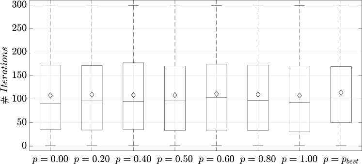
Figure 4. Number of iterations of ATheNA-SA ($p=1$), ATheNA-SM ($p=0$), and ATheNA ($0\leq p\leq 1$). Diamonds depict the average.

[Boxplots showing the number of iterations for different values of $p$.]Boxplots showing the number of iterations for different values of $p$. The plot has a separate column for each value of $p$ and a last column for $p_{best}$. The plot shows that for all the columns, the median number of iterations is around 100, with a slightly higher average number of iterations.

Results: The box plots in Figure 4 show the distribution in the number of iterations required by ATheNA-SA ($p=1$), ATheNA-SM ($p=0$), ATheNA-S ($0\leq p\leq 1$) and $\texttt{ATheNA-S}_{best}$ ($p=p_{best}$). The Wilcoxon rank sum test (McDonald, 2009) (Significance Level $\alpha=0.05$) confirms that there is no statistical difference between the median number of iterations $\texttt{ATheNA-S}_{avg}$, ATheNA-SA, and ATheNA-SM require to generate failure-revealing test cases. It also confirms that the median number of iterations $\texttt{ATheNA-S}_{best}$ requires to generate failure-revealing test cases is higher than the ones needed by ATheNA-SA and ATheNA-SM. However, as listed in Table 10, the difference in the number of iterations between $\texttt{ATheNA-S}_{best}$ and any other value of $p$ is at most $12$ iterations for the median and $6.1$ iterations for the average. The most computation-intensive model (F16) requires only $3s$ per iteration. Therefore, $12$ additional iterations correspond to less than a minute of running time. This overhead is negligible, considering that the development of CPS models usually takes months or years. Note that our results are not in contradiction with the results from RQ3 since (a) efficiency and effectiveness are two dimensions of the problem (being more effective in finding failure-revealing test cases within a given time budget does not require being more efficient), and (b) to generate the box plots we only considered the failure-revealing runs. Therefore, the number of runs considered for generating the box plots of $\texttt{ATheNA-S}_{avg}$ and $\texttt{ATheNA-S}_{best}$ is higher since they are more effective than ATheNA-SA and ATheNA-SM in generating failure-revealing runs (see # Samples in Table 10). For example, unlike ATheNA-SA and ATheNA-SM, $\texttt{ATheNA-S}_{avg}$ and $\texttt{ATheNA-S}_{best}$ generate failure-revealing test cases for CC4 requiring on average $260$ iterations each. We considered these failure-revealing runs in generating the box plots reported in Figure 4. This decision penalizes $\texttt{ATheNA-S}_{avg}$ and $\texttt{ATheNA-S}_{best}$ over ATheNA-SA and ATheNA-SM in assessing efficiency.

For our assumption-requirement combinations, the difference between the number of iterations required by ATheNA-SA, ATheNA-SM, and ATheNA-S to generate the failure-revealing test cases is not statistically relevant or negligible depending on the value assigned to the parameter $p$.

5.6. Usefulness — RQ5

To assess the usefulness of ATheNA-S, we evaluate its applicability in two case studies from the automotive and medical domains.

5.6.1. Automotive case study

Benchmark: Our automotive case study is the Simulink^® model of a hybrid-electric vehicle (HEV) developed for the EcoCAR Mobility Challenge (Eco, line), a competition sponsored by the U.S. Department of Energy (DOE, line), General Motors (GM, line), and MathWorks (Mat, line). The HEV motor converts electrical energy into mechanical energy. A software controller regulates the behavior of the motor.

The HEV model includes 4775 blocks. It consists of multiple subsystems built using Add-On components of Simulink^®, including Simscape (Simscape, line), Simscape Electrical (SimscapeElectrical, line), and Simscape Driveline (Driveline, line). The controller is modeled with Simulink^® Stateflow (Stateflow, line). The controller input is the speed demand, i.e., the required speed in Kph (kilometer per hour), and its output is the vehicle speed. The HEV model contains three input exemplars with the speed demand for three urban driving scenarios.

Methodology: To generate realistic driving scenarios, we considered one of the three urban driving scenario examples and slightly varied the speed demand. Specifically, we added the input signal delta_i_speed to the HEV model that represents the variation applied to the speed demand of the urban driving scenario we considered. We set the value $400$s for the simulation time since it is the simulation time provided for the HEV model.

To use ATheNA-S, we first needed to design assumptions for the delta_i_speed input signal. We set $[0,4]$Kph as the value range for the assumption since it is a sufficiently small range for the variation of the speed demand. We considered five control points to ensure speed variations occur every $100$s. We set the pchip interpolation function (PCHIP, line) since it generates smooth and continuous signals for the variations of the speed demand.

The requirement we considered specifies that the difference between the desired speed and the speed of the vehicle after $0.7$s shall be lower than a threshold value. We declared an output signal delta_o_speed representing the difference between the vehicle speed and the desired demand $0.7$s before. Then, we expressed the requirement in STL as $\mathcal{G}_{[0,400]}(\texttt{delta\_o\_speed}<\texttt{threshold})$. The temporal operator $\mathcal{G}_{[0,400]}$ requires the value of delta_o_speed to be lower than the threshold value within the interval $[0,400]$s. We set $3$Kph as the threshold value since, for the urban driving scenario we considered, delta_o_speed is always lower than this value.

We prioritized inputs that generated considerable changes for the speed demand since we believed that these inputs were likely to lead to a violation of our requirement. Therefore, we define a manual fitness function that returns a value that decreases as the average distance between consecutive control points increases. We used the implementation for the method athenaFitness from Listing LABEL:listingMatlab and set $0.5$ as the value for $p$ to equally prioritize the manual and the automatic fitness functions. We set the value to $300$ for the number of iterations. Then, we ran ATheNA-S once. As expected, ATheNA-S could not generate any failure-revealing test case. We injected a representative fault in the model: we changed the threshold that makes the car switch from the Cruise_mode to the Accelerate_mode by $50\%$. We then ran ATheNA-S again and checked whether it could generate failure-revealing test cases for the faulty model.

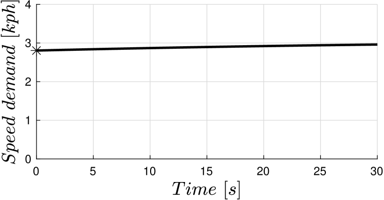
(a) Failure-revealing speed demand variation for the HEV model.

[Plot of the Speed demand variation.]Plot of the Speed demand variation for the first 30 seconds of simulation. The plot shows an almost constant signal at 3 kph.

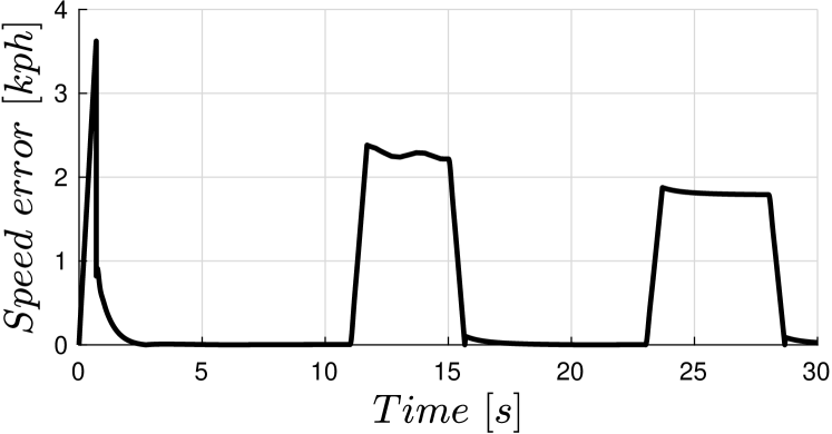
(b) Output signals for the HEV model for the input of Figure 5(a).

[Plot of the Speed error.]Plot of the Speed error for the first 30 seconds of simulation. The plot shows a peak in the signal at the beginning of the simulation, that exceeds 3 kph.

Figure 5. Example input and output for the Hybrid Electric Vehicle (HEV) Simulink^® model for the interval $[0,30]s$.

Results: ATheNA-S generated a failure-revealing test in $12$ iterations requiring $199$s ($\approx 3$min). Figure 5 shows a portion of the failure-revealing input and output signals. The failure-revealing test case shows that if the speed demand changes substantially within the first $5$ seconds of the simulation, the controller cannot keep the difference between the vehicle speed and the desired demand $0.7$s before within the desired threshold ($3$Kph). The cause of the problem was the change we made to the model: increasing the threshold that makes the car switch from the Cruise_mode to the Accelerate_mode by $50\%$ causes a problem when there is a variation of the speed at the beginning of the simulation.

5.6.2. Medical case study

Benchmark: Our medical case study is a mechanical ventilator (Miller, line) developed by MathWorks. The mechanical ventilator assists in the breathing of patients. The model we consider includes 241 blocks and consists of a real-time controller and a system model. The real-time controller is modeled in Simulink^® Stateflow (Stateflow, line). The system model includes the lungs and trachea of the patient. This example provides a starting point for designers working on ventilators, showing how to interface a real-time controller and a system model.

Methodology: We considered muscle pressure, body temperature, and room temperature as external inputs. The muscle pressure signal estimates the total inspiratory muscle pressure of a patient (Pleil et al., 2021). The body temperature and the room temperature are, respectively, the temperature of the body of the patient and the room.

The assumptions we considered for our input signals are as follows. We set $[0,0.05]$bar, $[35,39]^{\circ}$C, and $[18,25]^{\circ}$C as value range for the muscle pressure, body temperature, and room temperature external inputs. The maximum muscle pressure is the expiratory pressure for an average healthy adult woman (Lausted et al., 2006); the body and room temperature are assigned to reasonable value ranges. We considered two control points for the muscle pressure and used a step function as an interpolation function to simulate the sudden changes in the inhaling activity of the patient. We used two constant values for the body and room temperatures since we assumed these values do not change over the simulation time ($30$s).

The requirement specifies that the mechanical ventilator should ensure that the internal pressure of the patient’s respiratory system is below a threshold value and that the limits of the lung volume are not exceeded. We express this requirement in STL as $\mathcal{G}_{[0,30]}(\texttt{pressure}\leq\texttt{threshold}\land\texttt{min\_volume}\leq\texttt{volume}\leq\texttt{max\_volume})$. The temporal operator $\mathcal{G}_{[0,30]}$ requires the value of the pressure (pressure) and the lung volume (volume) to be within the threshold values during the interval $[0,30]$s. We set $30cm_{H_{2}O}$ as the threshold value for the pressure since it is the recommended threshold for the Plateau Pressure (PP) to avoid lung injury in patients connected to a mechanical ventilator (The Acute Respiratory Distress Syndrome Network, 2000). We set $0$L and $6$L as minimum and maximum threshold values for the lung volume since $6$L is the average lung capacity for an adult (Delgado and Bajaj, 2022).

Our manual fitness function prioritizes inputs with high initial and low final pressure as well as high body temperature. We select this fitness function to test if the ventilator can handle sudden changes in the state of the patient, i.e., suddenly stopping the inhaling activity, and can ensure its safety in critical conditions, like high body temperature and irregular breathing patterns.

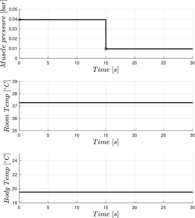
(a) Failure-revealing input signals for the MV model.RandomWord

[Plot of the inputs of the Mechanical Ventilator.]Plot of the inputs of the Mechanical Ventilator. The plots show a constant body temperature of $37$ degrees, a room temperature of $19$ degrees, and a step muscular pressure going from $0.04~{}bar$ to $0.01~{}bar$ at $15$ seconds.

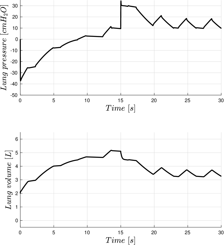
(b) Output signals for the MV model for the input of Figure 6(a).

[Plot of the outputs of the Mechanical Ventilator.]Plot of the outputs of the Mechanical Ventilator. The plots show a sudden increase in lung pressure at $15$ seconds.

Figure 6. Example input and output for the Mechanical Ventilator (MV) Simulink^® model.

Results: ATheNA-S generated a failure-revealing test in $8$ iterations requiring $452$s ($\approx 7.5$min). Figure 6 shows a portion of the failure-revealing input and output signals. The figure shows that when the voluntary breathing of the patient is abruptly reduced (see time instant $t=15s$), the mechanical ventilator cannot guarantee that the internal pressure of the respiratory system of the patient is below a threshold value ($30cm_{H_{2}O}$); it reaches $34.3cm_{H_{2}O}$ at time instant $15.0$. Therefore, although the ventilator relies on the patient’s inhalation and exhalation cycle to control the pressure, a sudden change can lead to a violation of the pressure threshold, which could damage the respiratory tract of the patient. We remark that although MathWorks experts developed the model, they did not ensure the correctness of their model — the goal of the model is to provide a starting point for designers working on ventilators, showing how to interface a real-time controller and a system model.

ATheNA-S was able to compute a failure-revealing test case for two case studies from the automotive and medical domains. ATheNA-S returned these test cases respectively after $12$ and $8$ iterations that required approximately three and seven minutes of computation.

6. Discussion and Threats to Validity

For the benchmark models and requirements we considered, our results show that ATheNA-S is more effective in detecting failure-revealing test cases than the baseline frameworks with no significant runtime performance overhead. Additionally, ATheNA-S was able to generate a failure-revealing test case for CC4 that the baselines could not find. Finally, ATheNA-S was able to generate a failure-revealing test case for our case studies. Based on these results, a possible workflow for the use of ATheNA is as follows: Engineers should initially use SBST frameworks based on automated fitness functions since they do not require manual effort to be defined and may already return failure-revealing test cases. If no failure-revealing test case is detected, engineers should use SBST frameworks based on manually defined fitness functions since they guide the search toward portions of the input domain more likely to contain failures. Finally, engineers should use SBST frameworks that combine automatically generated and manually defined fitness functions and can detect failures other frameworks cannot find. Note that this workflow is only one of the possible workflows for using ATheNA, which is proposed based on the results of our empirical investigation. Future experiments and empirical analysis may confirm the benefits of this workflow in practice or suggest new workflow usages for ATheNA.

In the following section, we reflect on the novelty of the proposed solution, the definition and use of the manual fitness functions, the applicability of the automatic fitness functions, and ATheNA in general. Finally, we discuss the threats to the validity of our results.

Novelty: Developing techniques that enable the generation of failure-revealing test cases effectively and efficiently is a widely known software engineering problem (Papadakis et al., 2019; Ali et al., 2010). No existing solution enables engineers to combine automatically generated and manually defined fitness functions. Therefore, ATheNA is a significant technical contribution: it improves the research literature and practice by introducing a novel and new solution and extensively evaluates the solution on existing benchmarks from the literature and two representative case studies.

Manual fitness function definition and use: To define the manual fitness function, engineers need to consider the requirement under analysis and the model behaviors, and guide the search toward portions of the input domains that more likely contain failure-revealing test cases. We designed manual fitness functions by reverse engineering the models, considering each requirement, and identifying portions of the input domains that we believed more likely contained failure-revealing test cases. ATheNA-SM is executed for each assumption-requirement combination — when a specific combination is considered, the automatically-generated and manually-derived fitness functions associated with that requirement are considered. Therefore, the manual fitness function designed for one requirement cannot harm the search with respect to another requirement. Even if manual fitness functions are defined for each requirement, manual fitness functions can be reused (and be useful) for multiple requirements. For example, as shown in Table 4, the requirements CC1 and CC3 share the same manual fitness function.

Applicability of the automatic fitness functions: Although ATheNA-S considers automatic fitness functions obtained from requirements specified in STL, our approach is largely applicable. Simulink^® provides several tools that enable engineers to formalize requirements, such as Test Assessment blocks (MathWorks, line), which were also considered as inputs for SBST of CPS (Formica et al., 2022). ATheNA can be extended to support any other automatic fitness function. For example, we plan to integrate ATheNA-S with an approach we recently proposed that automatically converts Test Assessment blocks into automatic fitness functions (Formica et al., 2022). This extension will enable our framework to support requirements specified using Test Assessment blocks that are natively integrated into Simulink^®.

ATheNA can be instantiated using different automated translations from STL to fitness functions. Our implementation, ATheNA-S relies on the translation used by S-Taliro and inherits the same limitations. As previously mentioned, we selected S-Taliro due to its recent classification as ready for industrial development, and its use in several industrial systems. Our solution can be extended by considering other automated translations from the literature (e.g., (Fainekos and Pappas, 2009, 2006; Donzé and Maler, 2010; Pant et al., 2017; Menghi et al., 2019)). An extensive comparison of these solutions is out of scope.

Automatically-generated fitness functions for multiple requirements can be obtained via ATheNA by writing an STL formula representing the Conjunction of the requirements and running the automated translation. For example, the automatically-generated fitness function for requirement AT6abc is obtained by generating the conjunction of requirements AT6a, AT6b, and AT6c and by running the automated translation. These requirements can benefit from dedicated automated fitness functions, such as (Peltomäki and Porres, 2022).

Applicability of ATheNA: Our running example concerning the automatic transmission model from Section 3 is from the automotive domain. However, as shown in our evaluation (Section 5), ATheNA is applicable in many CPS domains, including energy (Jin et al., 2014) and medical (Sankaranarayanan and Fainekos, 2012). Section 5 presents both the automatically-generated and manually-derived fitness functions considered for our benchmark models. Other instances of ATheNA can target different types of artifacts, e.g., source code or other types of models. Finally, our results show the benefits and complementarity of automatically-generated and manually-derived fitness functions in the context of SBST of CPS: even if a formal requirement was available for CC4, the search driven by either the automatic or the manual fitness functions did not return any failure-revealing test cases. On the contrary, the combination of the two returned a set of failure revealing test cases.

The scalability of the proposed technique depends on many factors: the number of input signals, the number of control points, their input ranges, the number of blocks of the model and the time required to simulate it. We can not claim that a higher number of input signals will necessarily negatively impact the scalability of the proposed technique, since those additional input signals may simplify the detection of failure revealing test cases. More empirical studies, like the one presented in this paper, can assess how the number of input signals, the number of control points, their input ranges, the number of blocks of the model and the time required to simulate it influence the scalability of the SBST frameworks.

Our results provide empirical evidence supporting the usefulness of manual fitness functions. This result is not obvious: the use of manual fitness functions can worsen the search process. For example, ATheNA did not improve the search process compared to S-Taliro for one of the benchmarks (i.e., NN-R), and, for another, using ATheNA worsens the performance compared to S-Taliro (i.e., WT3-R). Therefore, our results are significant. They provide empirical evidence that, for our benchmark, the manual fitness functions improved the search process.

The first author designed the manual fitness functions we considered in our experimentation. The preliminary experiment to assess the effort required to write manual fitness functions relies on two subjects. Although our study considers a limited number of participants, it is one of the first attempts to perform such a user study for SBST tools in the Simulink^® domain. Future work can extend our analysis by considering a larger number of participants and investigating the tool’s usability by end-users in this domain.

The general framework presented in Section 2 can be instantiated by considering different fitness functions, including branch distance (see for example (Arcuri, 2010)). In our implementation (Section 4), the fitness function automatically generated from the requirement relies on the notion of robustness. Similarly to branch distance, robustness evaluates how far a predicate is from obtaining its opposite value. However, unlike branch distance, the robustness metric is evaluated on predicates that change their value over time, and therefore provide the semantics for logical temporal operators, such as globally and eventually.

ATheNA is a framework for black-box testing: it assumes that the internal structure of the model is unknown. The search algorithm explores the input domain looking for failure-revealing test cases. While fitness landscape analysis (e.g., (Aleti et al., 2017; Campos et al., 2018; Albunian et al., 2020; Joffe and Clark, 2019)) can help engineers in designing the manual fitness function, we did not use it not to bias our evaluation; using the fitness landscape analysis to support the design of the manual fitness function is an interesting direction for future work that can further improve our results and is outside the scope of this work.

External Validity: The selection of the models and requirements is a threat to the external validity of our results. However, the benchmark models considered in RQ1 and RQ2 (a) were extensively used in the SBST literature (e.g., (Ernst et al., 2022; Fehnker and Ivančić, 2004; Jin et al., 2014; Menghi et al., 2020; Fainekos et al., 2019; Donzé and Maler, 2010)), (b) are representative of different CPS systems, i.e., AT, AFC and CC are from the automotive domain, NN is from the ML domain, WT is from the electrical domain, and F16 is from the aerospace domain, (c) some of the models were developed by engineers working in the industry, i.e., AFC is from Toyota (Jin et al., 2014). The case studies used to answer RQ5 are large and complex case studies representative of industrial systems developed by MathWorks (Mat, line) and linked to the EcoCAR Mobility Challenge (Eco, line), a competition sponsored by the U.S. Department of Energy (DOE, line), General Motors (GM, line).

The reverse-engineering process we used to define the manual fitness functions for ATheNA-SM (see Section 5.4), the fitness function of ATheNA-S, and the fault we injected are a threat to the external validity of our results. However, the results of ATheNA-SM and ATheNA-S are likely to improve when the designers of the fitness functions are knowledgeable about the domain and engineered the Simulink^® models.

ATheNA-S explicitly targets Simulink^® models. Other instances of ATheNA can target different model types or software programs. We conjecture that our results are also generalizable to these domains. More empirical studies, such as those presented in this paper, will determine whether our conjecture holds.

The selection of the automatically-generated, manually-derived, and ATheNA fitness functions threat the external validity of our results. Although the ATheNA fitness function relies on the value of the parameter $p$ to linearly combine the value of automatically-generated and manually-derived fitness functions, other ATheNA fitness functions can be used by engineers (as detailed in Section 4). Section 5.3 experiments with different values of $p$ and discusses how we selected the value of $p$.

Internal Validity: The values assigned to the configuration parameters of our tools are a threat to the internal validity of our results. However, our configuration does not favor any of the frameworks as the common configuration parameters of ATheNA-SA, ATheNA-SM, and ATheNA share the same values.

The current experiments demonstrate that ATheNA outperforms ATheNA-SA and ATheNA-SM. While it is possible to address a search problem by manually defining ad-hoc fitness functions in theory, Section 5.2 showed that this was also possible in practice. The procedure we used to define the manual fitness functions (Section 5.2) required us to reverse engineer the model. We were not the designers of the models. Section 5.3 defined the procedure we used to select the value for the parameter $p$ of the ATheNA fitness function. In practice, engineers are more knowledgeable about their models and can select more appropriate values for the parameter $p$ depending on many factors, such as the development stage and the likelihood of finding failure by prioritizing the manual and the automatic fitness functions. During earlier development stages, engineers will likely prioritize explorative search by relying on the automatic fitness function and move toward exploitative search that depends on the manual fitness function as the design progresses and they become more aware of areas of the input domain that are more critical for the satisfaction of the requirement. Therefore, the methodology we followed in our evaluation penalizes our approach, and the current experimental method confirms the hypothesis on the effectiveness of ATheNA.

7. Related Work

Despite the vast research literature on SBST and the considerable number of surveys on the topic (e.g.,  (Ali et al., 2010; Khari and Kumar, 2019; Nelson et al., 2009; Klück et al., 2019; Harman et al., 2015; Brunetto et al., 2021)), we did not find any existing work classifying fitness functions into automatically generated and manually defined. In addition, we are not aware of any work proposing a framework that combines these two types of fitness functions. Therefore, this section summarizes related work targeting automatically generated fitness functions, manually defined fitness functions, and multi-objective fitness functions.

Automated generation of fitness function techniques often compute fitness functions from logic-based specifications (e.g., (Fainekos and Pappas, 2009, 2006; Donzé and Maler, 2010; Pant et al., 2017; Menghi et al., 2019)). Well established SBST tools, such as Breach (Donzé, 2010), S-Taliro (Annpureddy et al., 2011), Aristeo (Menghi et al., 2020), and FalStar (Waga, 2020), rely on these fitness functions. For each atomic proposition, these fitness functions typically compute a value indicating a satisfaction degree for the proposition at every time instant. There are alternative ways to compute fitness values associated with temporal operators, such as the use of min and max operators (Fainekos and Pappas, 2009, 2006), distance operators computing smooth approximations of the min and max operators (e.g., (Pant et al., 2017)), arithmetic and geometric mean along a time interval (e.g., (Mehdipour et al., 2019; Lindemann and Dimarogonas, 2019; Varnai and Dimarogonas, 2020)), cumulative values over a time horizon (e.g., (Haghighi et al., 2019)). Some approaches also consider perturbations that may shift the signal values over time to compute the fitness value (e.g., (Donzé and Maler, 2010)).

A variety of manually defined fitness functions was proposed in the literature. Manually defined fitness functions can guide the search to produce test outputs with diverse shapes (Matinnejad et al., 2016a), maximize or minimize the outputs of a system characterizing its critical behavior (Ben Abdessalem et al., 2018), maximize diversity in output signals (Matinnejad et al., 2016b), quantify the difference between a reference and an output signal (Arrieta et al., 2021), and minimize the difference between the expected and simulated behavior of a CPS (Humeniuk et al., 2021). Many manually defined fitness functions were also proposed to guide SBST frameworks that analyze software code. For example, some recent manually defined fitness functions measure line coverage, input coverage, output coverage (e.g., (Kechagia et al., 2019)), branch distances (e.g., (Panichella et al., 2018)), test length, method sequence diversity, and crash distance (Derakhshanfar et al., 2020), the cumulative number of defects and the total amount of code to inspect (Panichella et al., 2016). Manually defined fitness functions can also compute exploration measures (Matinnejad et al., 2014), and combine coverage-based and feature interaction measures (Abdessalem et al., 2018).

Differently from these works, we proposed a framework that combines automatically generated and manually defined fitness functions and showed the benefits of our framework by considering a large benchmark made by seven models and $27$ requirements and two complex case studies from the automotive and medical domains.

Multi-objective fitness functions are extensively studied by the research literature (see for example  (Li and Yao, 2019; Wu et al., 2022; Sayyad and Ammar, 2013; Ali et al., 2020; Ramirez et al., 2019; Li et al., 2020; Ramirez et al., 2018; Nuh et al., 2021) for recent surveys). For example, SBST frameworks guided by multi-objective search are used for machine learning and automotive systems (e.g., (Gambi et al., 2019; Klischat and Althoff, 2019; Haq et al., 2022; Ben Abdessalem et al., 2016; Riccio and Tonella, 2020)), test case prioritization (e.g., (Pradhan et al., 2019, 2018)), software refactoring (e.g., (Mohan and Greer, 2019)), software energy consumption (e.g., (Álvarez et al., 2016)), generation of software assumptions (e.g., (Gaaloul et al., 2022, 2020)), and many others uses. These frameworks use fitness functions based on more than one objective to guide the search exploration. Within multi-objective fitness functions, optimizing one objective may harm another. Therefore, there is no single optimal solution for these problems, but a set of non-dominated optimal solutions called Pareto Front (Wright et al., 1999). Therefore, SBST usually aims to detect (a solution belonging to) the Pareto Front. Quality Indicators (Li and Yao, 2019) are often used to compare the performance of these algorithms and are chosen depending on the specific application. SBST frameworks that rely on multi-objective fitness functions also exist for Matlab and Simulink^® (e.g., (Toffolo and Lazzaretto, 2002)).

Our solution shares some similarities with these works: The fitness function obtained by combining the automatic and the manual fitness functions is a multi-objective fitness function. However, our work is significantly different since it is the first work that enables the combination of manual and automatic fitness functions. Proposing a framework that enables engineers to use manual and automatic fitness functions is a significant contribution. As we have shown in our evaluation, our solution is reusable and applicable in different domains. Such support helps engineers find failure-revealing test cases they can not find with other existing approaches.

8. Conclusion and Future Work

We presented ATheNA, a novel SBST framework that combines automatically generated and manually defined fitness functions. We defined ATheNA-S, an instance of ATheNA that supports Simulink^® models. We considered two versions of ATheNA-S to assess its benefits in generating failure-revealing test cases. The two versions of ATheNA-S we considered are preferable over the baseline tools for respectively $\approx 79\%$ and $100\%$ of our assumption-requirement combinations. They generated more failure-revealing test cases than one baseline SBST framework that relies on automatic fitness functions (+$7.9\%$ and +$11.9\%$) and another based on manually defined fitness functions (+$8.1\%$ and +$12.1\%$). ATheNA-S did not show statistically significant differences in efficiency compared with the baseline tools. Finally, ATheNA-S generated a failure-revealing test case for two large representative automotive and medical case studies. We discussed the impacts of our results on software engineering practices, and suggested a workflow that combines ATheNA and SBST frameworks driven by automatically generated and manually defined fitness functions.

We plan to further support engineers with techniques that automatically infer the value assigned to the parameter $p$ and dynamically change the prioritization of the automatically generated and manually defined fitness functions at run-time in future work.

Data Availability

A replication package containing all of our data, test results, and models is publicly available (Mat, 2023).

- (1)
- DBL (2021) 2021. Computer Safety, Reliability, and Security (SAFECOMP). Springer. https://doi.org/10.1007/978-3-030-83903-1
- Mat (line) 2022 [Online]. MathWorks. Retrieved April 2022 from https://www.mathworks.com
- Eco (line) 2022 [Online]. The EcoCAR Mobility Challenge . Retrieved April 2022 from https://it.mathworks.com/academia/student-competitions/ecocar.html
- Mat (2023) 2023. Replication Package. https://doi.org/10.5281/zenodo.8309516
- Abbas et al. (2014a) Houssam Abbas, Bardh Hoxha, Georgios Fainekos, and Koichi Ueda. 2014a. Robustness-guided temporal logic testing and verification for stochastic cyber-physical systems. In International Conference on Cyber Technology in Automation, Control and Intelligent. IEEE, 1–6.
- Abbas et al. (2014b) Houssam Abbas, Andrew Winn, Georgios Fainekos, and A Agung Julius. 2014b. Functional gradient descent method for metric temporal logic specifications. In American Control Conference. IEEE, 2312–2317.
- Abdessalem et al. (2018) Raja Ben Abdessalem, Annibale Panichella, Shiva Nejati, Lionel C Briand, and Thomas Stifter. 2018. Testing autonomous cars for feature interaction failures using many-objective search. In International Conference on Automated Software Engineering. IEEE, 143–154.
- Albunian et al. (2020) Nasser Albunian, Gordon Fraser, and Dirk Sudholt. 2020. Causes and effects of fitness landscapes in unit test generation. In Genetic and Evolutionary Computation Conference. 1204–1212.
- Aleti et al. (2017) Aldeida Aleti, Irene Moser, and Lars Grunske. 2017. Analysing the fitness landscape of search-based software testing problems. Automated Software Engineering 24, 3 (2017), 603–621. https://doi.org/10.1007/s10515-016-0197-7
- Ali et al. (2020) Shaukat Ali, Paolo Arcaini, Dipesh Pradhan, Safdar Aqeel Safdar, and Tao Yue. 2020. Quality indicators in search-based software engineering: an empirical evaluation. ACM Transactions on Software Engineering and Methodology 29, 2 (2020), 1–29. https://doi.org/10.1145/3375636
- Ali et al. (2010) Shaukat Ali, Lionel C. Briand, Hadi Hemmati, and Rajwinder Kaur Panesar-Walawege. 2010. A Systematic Review of the Application and Empirical Investigation of Search-Based Test Case Generation. IEEE Transactions on Software Engineering 36, 6 (2010), 742–762. https://doi.org/10.1109/TSE.2009.52
- Almulla and Gay (2020) Hussein Almulla and Gregory Gay. 2020. Learning How to Search: Generating Exception-Triggering Tests Through Adaptive Fitness Function Selection. In International Conference on Software Testing, Validation and Verification. IEEE, 63–73.
- Altinger et al. (2014) Harald Altinger, Franz Wotawa, and Markus Schurius. 2014. Testing Methods Used in the Automotive Industry: Results from a Survey. In Workshop on Joining AcadeMiA and Industry Contributions to Test Automation and Model-Based Testing. ACM, 1–6.
- Álvarez et al. (2016) Josefa Díaz Álvarez, José L Risco-Martín, and J Manuel Colmenar. 2016. Multi-objective optimization of energy consumption and execution time in a single level cache memory for embedded systems. Journal of Systems and Software 111 (2016), 200–212. https://doi.org/10.1016/j.jss.2015.10.012
- Amal et al. (2014) Boukhdhir Amal, Marouane Kessentini, Slim Bechikh, Josselin Dea, and Lamjed Ben Said. 2014. On the Use of Machine Learning and Search-Based Software Engineering for Ill-Defined Fitness Function: A Case Study on Software Refactoring. In International Symposium on Search-Based Software Engineering. Springer, 31–45.
- Annpureddy et al. (2011) Yashwanth Annpureddy, Che Liu, Georgios Fainekos, and Sriram Sankaranarayanan. 2011. S-TaLiRo: A Tool for Temporal Logic Falsification for Hybrid Systems. In Tools and Algorithms for the Construction and Analysis of Systems. Springer, 254–257.
- ARCH (line) ARCH 2021 [Online]. International Competition on Verifying Continuous and Hybrid Systems. Retrieved April 2022 from https://cps-vo.org/group/ARCH/FriendlyCompetition
- Arcuri (2010) Andrea Arcuri. 2010. It does matter how you normalise the branch distance in search based software testing. In International Conference on Software Testing, Verification and Validation. IEEE, 205–214.
- Arcuri and Briand (2011) Andrea Arcuri and Lionel Briand. 2011. A practical guide for using statistical tests to assess randomized algorithms in software engineering. In International Conference on Software Engineering. ACM, 1–10.
- ARIsTEOWeb (line) ARIsTEOWeb 2022 [Online]. ARIsTEO — AppRoxImation-based TEst generatiOn. Retrieved April 2022 from https://github.com/SNTSVV/ARIsTEO
- Arrieta et al. (2020) Aitor Arrieta, Joseba A. Agirre, and Goiuria Sagardui. 2020. A Tool for the Automatic Generation of Test Cases and Oracles for Simulation Models Based on Functional Requirements. In International Conference on Software Testing, Verification and Validation Workshops. ACM/IEEE, 1–5.
- Arrieta et al. (2021) Aitor Arrieta, Jon Ayerdi, Miren Illarramendi, Aitor Agirre, Goiuria Sagardui, and Maite Arratibel. 2021. Using Machine Learning to Build Test Oracles: an Industrial Case Study on Elevators Dispatching Algorithms. In International Conference on Automation of Software Test. IEEE, 30–39.
- ATBenchmark (line) ATBenchmark 2022 [Online]. Modeling an Automatic Transmission Controller. Retrieved April 2022 from https://www.mathworks.com/help/simulink/slref/modeling-an-automatic-transmission-controller.html
- ATheNA Replication Package (line) ATheNA Replication Package 2023 [Online]. ATheNA. Retrieved March 2023 from https://github.com/ATheNA-SBST/ATheNA
- ATheNAAddOn (line) ATheNAAddOn 2022 [Online]. ATheNA Add-on. Retrieved August 2022 from https://it.mathworks.com/matlabcentral/fileexchange/116095-athena?s_tid=srchtitle_athena_1
- AUT (line) AUT 2022 [Online]. Automotive Electrical System Simulation and Control. Retrieved April 2022 from https://it.mathworks.com/matlabcentral/fileexchange/25674-automotive-electrical-system-simulation-and-control
- Bajaj and Sangwan (2019) Anu Bajaj and Om Prakash Sangwan. 2019. A Systematic Literature Review of Test Case Prioritization Using Genetic Algorithms. IEEE Access 7 (2019), 126355–126375. https://doi.org/10.1109/ACCESS.2019.2938260
- Ben Abdessalem et al. (2016) Raja Ben Abdessalem, Shiva Nejati, Lionel C Briand, and Thomas Stifter. 2016. Testing advanced driver assistance systems using multi-objective search and neural networks. In IEEE/ACM International Conference on Automated Software Engineering. 63–74.
- Ben Abdessalem et al. (2018) Raja Ben Abdessalem, Shiva Nejati, Lionel C. Briand, and Thomas Stifter. 2018. Testing Vision-Based Control Systems Using Learnable Evolutionary Algorithms. In International Conference on Software Engineering. ACM, 1016–1026.
- Boll et al. (2021) Alexander Boll, Florian Brokhausen, Tiago Amorim, Timo Kehrer, and Andreas Vogelsang. 2021. Characteristics, potentials, and limitations of open-source Simulink projects for empirical research. Software and Systems Modeling 20, 6 (2021), 2111–2130. https://doi.org/10.1007/s10270-021-00883-0
- Brunetto et al. (2021) Matteo Brunetto, Giovanni Denaro, Leonardo Mariani, and Mauro Pezzè. 2021. On introducing automatic test case generation in practice: A success story and lessons learned. Journal of Systems and Software 176 (2021), 110933. https://doi.org/10.1016/j.jss.2021.110933
- Campos et al. (2018) José Campos, Yan Ge, Nasser Albunian, Gordon Fraser, Marcelo Eler, and Andrea Arcuri. 2018. An empirical evaluation of evolutionary algorithms for unit test suite generation. Information and Software Technology 104 (2018), 207–235. https://doi.org/10.1016/j.infsof.2018.08.010
- Cohen and Belta (2021) Max H. Cohen and Calin Belta. 2021. Model-Based Reinforcement Learning for Approximate Optimal Control with Temporal Logic Specifications. In International Conference on Hybrid Systems: Computation and Control. ACM, 1–12.
- Delgado and Bajaj (2022) Benjamin J. Delgado and Tushar Bajaj. 2022. Physiology, Lung Capacity. StatPearls Publishing, Treasure Island (FL). http://europepmc.org/books/NBK541029
- Derakhshanfar et al. (2020) Pouria Derakhshanfar, Xavier Devroey, Andy Zaidman, Arie van Deursen, and Annibale Panichella. 2020. Good Things Come In Threes: Improving Search-based Crash Reproduction With Helper Objectives. In International Conference on Automated Software Engineering. IEEE/ACM, 211–223.
- DOE (line) DOE 2022 [Online]. United States Department of Energy. Retrieved April 2022 from httpshttps://www.energy.gov/
- Donzé (2010) Alexandre Donzé. 2010. Breach, A Toolbox for Verification and Parameter Synthesis of Hybrid Systems. In Computer Aided Verification. Springer, 167–170.
- Donzé and Maler (2010) Alexandre Donzé and Oded Maler. 2010. Robust Satisfaction of Temporal Logic over Real-Valued Signals. In Formal Modeling and Analysis of Timed Systems. Springer, 92–106.
- Driveline (line) Driveline 2022 [Online]. Simscape Driveline Model and simulate rotational and translational mechanical systems. Retrieved April 2022 from https://www.mathworks.com/products/simscape-driveline.html
- Duan et al. (2018) Pengfei Duan, Ying Zhou, Xufang Gong, and Bixin Li. 2018. A systematic mapping study on the verification of cyber-physical systems. IEEE Access 6 (2018), 59043–59064. https://doi.org/10.1109/ACCESS.2018.2872015
- Ernst et al. (2022) Gidon Ernst, Paolo Arcaini, Georgios Fainekos, Federico Formica, Jun Inoue, Tanmay Khandait, Mohammad Mahdi Mahboob, Claudio Menghi, Giulia Pedrielli, Masaki Waga, Yoriyuki Yamagata, and Zhenya Zhang. 2022. ARCH-COMP 2022 Category Report: Falsification with Ubounded Resources. In International Workshop on Applied Verification of Continuous and Hybrid Systems (ARCH22) (EPiC Series in Computing, Vol. 90). EasyChair, 204–221.
- Ernst et al. (2019) Gidon Ernst, Sean Sedwards, Zhenya Zhang, and Ichiro Hasuo. 2019. Fast falsification of hybrid systems using probabilistically adaptive input. In International Conference on Quantitative Evaluation of Systems: (QEST). Springer, 165–181.
- Ernst et al. (2021) Gidon Ernst, Sean Sedwards, Zhenya Zhang, and Ichiro Hasuo. 2021. Falsification of hybrid systems using adaptive probabilistic search. Transactions on Modeling and Computer Simulation 31, 3 (2021), 1–22. https://doi.org/10.1145/3459605
- Fainekos et al. (2019) Georgios Fainekos, Bardh Hoxha, and Sriram Sankaranarayanan. 2019. Robustness of Specifications and Its Applications to Falsification, Parameter Mining, and Runtime Monitoring with S-TaLiRo. In International Conference on Runtime Verification. Springer, 27–47.
- Fainekos and Pappas (2006) Georgios E Fainekos and George J Pappas. 2006. Robustness of temporal logic specifications. In Formal Approaches to Software Testing and Runtime Verification. Springer, 178–192.
- Fainekos and Pappas (2009) Georgios E Fainekos and George J Pappas. 2009. Robustness of temporal logic specifications for continuous-time signals. Theoretical Computer Science 410, 42 (2009), 4262–4291. https://doi.org/10.1016/j.tcs.2009.06.021
- Fehnker and Ivančić (2004) Ansgar Fehnker and Franjo Ivančić. 2004. Benchmarks for hybrid systems verification. In International Workshop on Hybrid Systems: Computation and Control. Springer, 326–341.
- Formica et al. (2022) Federico Formica, Tony Fan, Akshay Rajhans, Vera Pantelic, Mark Lawford, and Claudio Menghi. 2022. Simulation-based Testing of Simulink Models with Test Sequence and Test Assessment Blocks. arXiv preprint (2022). https://doi.org/10.48550/arXiv.2212.11589
- Gaaloul et al. (2022) Khouloud Gaaloul, Claudio Menghi, Shiva Nejati, Lionel C. Briand, and Yago Isasi Parache. 2022. Combining Genetic Programming and Model Checking to Generate Environment Assumptions. IEEE Transactions on Software Engineering 48, 9 (2022), 3664–3685. https://doi.org/10.1109/TSE.2021.3101818
- Gaaloul et al. (2020) Khouloud Gaaloul, Claudio Menghi, Shiva Nejati, Lionel C. Briand, and David Wolfe. 2020. Mining Assumptions for Software Components Using Machine Learning. In European Software Engineering Conference and Symposium on the Foundations of Software Engineering. ACM, 159–171. https://doi.org/10.1145/3368089.3409737
- Gambi et al. (2019) Alessio Gambi, Marc Mueller, and Gordon Fraser. 2019. Automatically testing self-driving cars with search-based procedural content generation. In International Symposium on Software Testing and Analysis. 318–328.
- Garousi et al. (2018) Vahid Garousi, Michael Felderer, Çağrı Murat Karapıçak, and Uğur Yılmaz. 2018. Testing embedded software: A survey of the literature. Information and Software Technology 104 (2018), 14–45. https://doi.org/10.1016/j.infsof.2018.06.016
- GM (line) GM 2022 [Online]. General Motors. Retrieved April 2022 from https://www.gm.com/
- GMD (line) GMD 2022 [Online]. General Motors recalling 4.3 million vehicles for airbag defect. Retrieved April 2022 from https://www.cbc.ca/news/business/general-motors-recall-airbag-software-1.3755030
- Haghighi et al. (2019) Iman Haghighi, Noushin Mehdipour, Ezio Bartocci, and Calin Belta. 2019. Control from Signal Temporal Logic Specifications with Smooth Cumulative Quantitative Semantics. In Conference on Decision and Control. IEEE, 4361–4366.
- Haq et al. (2022) Fitash Ul Haq, Donghwan Shin, and Lionel Briand. 2022. Efficient online testing for DNN-enabled systems using surrogate-assisted and many-objective optimization. In International Conference on Software Engineering. 811–822.
- Harman and Clark (2004) M. Harman and J. Clark. 2004. Metrics are fitness functions too. In International Symposium on Software Metrics. IEEE, 58–69.
- Harman et al. (2015) Mark Harman, Yue Jia, and Yuanyuan Zhang. 2015. Achievements, Open Problems and Challenges for Search Based Software Testing. In International Conference on Software Testing, Verification and Validation. IEEE, 1–12.
- Hart and Ross (2001) Emma Hart and Peter Ross. 2001. Gavel-a new tool for genetic algorithm visualization. Transactions on Evolutionary Computation 5, 4 (2001), 335–348. https://doi.org/10.1109/4235.942528
- Honda (line) Honda 2022 [Online]. Honda recalls 1.4M U.S. vehicles for software, other problems. Retrieved April 2022 from https://www.nbcnews.com/business/consumer/honda-recalls-1-4m-u-s-vehicles-software-other-problems-n1251496
- Humeniuk et al. (2021) Dmytro Humeniuk, Giuliano Antoniol, and Foutse Khomh. 2021. Data Driven Testing of Cyber Physical Systems. In International Workshop on Search-Based Software Testing. IEEE/ACM, 16–19.
- Jin et al. (2014) Xiaoqing Jin, Jyotirmoy V Deshmukh, James Kapinski, Koichi Ueda, and Ken Butts. 2014. Powertrain control verification benchmark. In International conference on Hybrid systems: computation and control. ACM, 253–262.
- Joffe and Clark (2019) Leonid Joffe and David Clark. 2019. Directing a search towards execution properties with a learned fitness function. In Conference on Software Testing, Validation and Verification (ICST). IEEE, 206–216.
- Kapinski et al. (2016) James Kapinski, Jyotirmoy V Deshmukh, Xiaoqing Jin, Hisahiro Ito, and Ken Butts. 2016. Simulation-based approaches for verification of embedded control systems: An overview of traditional and advanced modeling, testing, and verification techniques. IEEE Control Systems Magazine 36, 6 (2016), 45–64. https://doi.org/10.1109/MCS.2016.2602089
- Kechagia et al. (2019) Maria Kechagia, Xavier Devroey, Annibale Panichella, Georgios Gousios, and Arie van Deursen. 2019. Effective and Efficient API Misuse Detection via Exception Propagation and Search-Based Testing. In International Symposium on Software Testing and Analysis. ACM SIGSOFT, 192–203.
- Khari and Kumar (2019) Manju Khari and Prabhat Kumar. 2019. An extensive evaluation of search-based software testing: a review. Soft computing 23, 6 (2019), 1933–1946. https://doi.org/10.1007/s00500-017-2906-y
- Kim and Moon (2002) Yong-Hyuk Kim and Byung-Ro Moon. 2002. Visualization of the fitness landscape, A steady-state genetic search, and schema traces. In Annual Conference on Genetic and Evolutionary Computation. Morgan Kaufmann, 686–686.
- Kim and Moon (2003) Yong-Hyuk Kim and Byung-Ro Moon. 2003. New usage of Sammon’s mapping for genetic visualization. In Genetic and Evolutionary Computation Conference. Springer, 1136–1147.
- Klischat and Althoff (2019) Moritz Klischat and Matthias Althoff. 2019. Generating critical test scenarios for automated vehicles with evolutionary algorithms. In Intelligent Vehicles Symposium (IV). IEEE, 2352–2358.
- Klück et al. (2019) Florian Klück, Martin Zimmermann, Franz Wotawa, and Mihai Nica. 2019. Performance Comparison of Two Search-Based Testing Strategies for ADAS System Validation. In International Conference on Testing Software and Systems. Springer, 140–156.
- LandRover (line) LandRover 2022 [Online]. Software bug causes Land Rover recall. Retrieved April 2022 from https://www.themanufacturer.com/articles/almost-36500-jlr-vehicles-recalled-in-china/
- Lausted et al. (2006) Christopher G. Lausted, Arthur T. Johnson, William H. Scott, Monique M. Johnson, Karen M. Coyne, and Derya C. Coursey. 2006. Maximum static inspiratory and expiratory pressures with different lung volumes. BioMedical Engineering OnLine 5, 1 (2006), 29. https://doi.org/10.1186/1475-925X-5-29
- Li et al. (2020) Miqing Li, Tao Chen, and Xin Yao. 2020. How to evaluate solutions in Pareto-based search-based software engineering: a critical review and methodological guidance. IEEE Transactions on Software Engineering 48, 5 (2020), 1771–1799. https://doi.org/10.1109/TSE.2020.3036108
- Li and Yao (2019) Miqing Li and Xin Yao. 2019. Quality evaluation of solution sets in multiobjective optimisation: A survey. ACM Computing Surveys (CSUR) 52, 2 (2019), 1–38. https://doi.org/10.1145/3300148
- Liebel et al. (2018) Grischa Liebel, Nadja Marko, Matthias Tichy, Andrea Leitner, and Jörgen Hansson. 2018. Model-based engineering in the embedded systems domain: an industrial survey on the state-of-practice. Software and Systems Modeling 17, 1 (2018), 91–113. https://doi.org/10.1007/s10270-016-0523-3
- Lindemann and Dimarogonas (2019) Lars Lindemann and Dimos V. Dimarogonas. 2019. Robust control for signal temporal logic specifications using discrete average space robustness. Automatica 101 (2019), 377–387. https://doi.org/10.1016/j.automatica.2018.12.022
- Majikes et al. (2013) John J Majikes, Rahul Pandita, and Tao Xie. 2013. Literature review of testing techniques for medical device software. In Medical Cyber-Physical Systems Workshop. Citeseer.
- Maler and Nickovic (2004) Oded Maler and Dejan Nickovic. 2004. Monitoring temporal properties of continuous signals. In Formal Techniques, Modelling and Analysis of Timed and Fault-Tolerant Systems. Springer, 152–166.
- Mathesen et al. (2019) Logan Mathesen, Shakiba Yaghoubi, Giulia Pedrielli, and Georgios Fainekos. 2019. Falsification of Cyber-Physical Systems with Robustness Uncertainty Quantification Through Stochic optimization with Adaptive Restart. In International Conference on Automation Science and Engineering. IEEE, 991–997.
- MathWorks (line) MathWorks. 2022 [Online]. Test Assessment. Retrieved September 2022 from https://www.mathworks.com/help/sltest/ref/testassessment.html Release R2022a..
- Matinnejad et al. (2014) Reza Matinnejad, Shiva Nejati, Lionel Briand, and Thomas Brcukmann. 2014. MiL Testing of Highly Configurable Continuous Controllers: Scalable Search Using Surrogate Models. In International Conference on Automated Software Engineering. ACM/IEEE, 163–174.
- Matinnejad et al. (2015) Reza Matinnejad, Shiva Nejati, Lionel Briand, Thomas Bruckmann, and Claude Poull. 2015. Search-based automated testing of continuous controllers: Framework, tool support, and case studies. Information and Software Technology 57 (2015), 705–722. https://doi.org/10.1016/j.infsof.2014.05.007
- Matinnejad et al. (2016a) Reza Matinnejad, Shiva Nejati, Lionel C. Briand, and Thomas Bruckmann. 2016a. Automated Test Suite Generation for Time-Continuous Simulink Models. In International Conference on Software Engineering. ACM/IEEE, 595–606.
- Matinnejad et al. (2016b) Reza Matinnejad, Shiva Nejati, Lionel C Briand, and Thomas Bruckmann. 2016b. Automated test suite generation for time-continuous simulink models. In International Conference on Software Engineering. ACM, 595–606.
- McDonald (2009) John H McDonald. 2009. Handbook of biological statistics. Vol. 2.
- Mehdipour et al. (2019) Noushin Mehdipour, Cristian-Ioan Vasile, and Calin Belta. 2019. Arithmetic-Geometric Mean Robustness for Control from Signal Temporal Logic Specifications. In American Control Conference. IEEE, 1690–1695.
- Menghi et al. (2020) Claudio Menghi, Shiva Nejati, Lionel Briand, and Yago Isasi Parache. 2020. Approximation-Refinement Testing of Compute-Intensive Cyber-Physical Models: An Approach Based on System Identification. In International Conference on Software Engineering. IEEE/ACM, 372–384.
- Menghi et al. (2019) Claudio Menghi, Shiva Nejati, Khouloud Gaaloul, and Lionel C Briand. 2019. Generating automated and online test oracles for simulink models with continuous and uncertain behaviors. In European software engineering conference and symposium on the foundations of software engineering. ACM, 27–38.
- Miller (line) Steve Miller. 2022 [Online]. Medical Ventilator Model in Simscape. Retrieved September 2022 from https://www.mathworks.com/matlabcentral/fileexchange/75012-medical-ventilator-model-in-simscape
- Mohan and Greer (2019) Michael Mohan and Des Greer. 2019. Using a many-objective approach to investigate automated refactoring. Information and Software Technology 112 (2019), 83–101. https://doi.org/10.1016/j.infsof.2019.04.009
- Nejati et al. (2023) Shiva Nejati, Lev Sorokin, Damir Safin, Federico Formica, Mohammad Mahdi Mahboob, and Claudio Menghi. 2023. Reflections on Surrogate-Assisted Search-Based Testing: A Taxonomy and Two Replication Studies based on Industrial ADAS and Simulink Models. Information and Software Technology 163 (2023), 107286. https://doi.org/10.1016/j.infsof.2023.107286
- Nelson et al. (2009) Andrew L. Nelson, Gregory J. Barlow, and Lefteris Doitsidis. 2009. Fitness functions in evolutionary robotics: A survey and analysis. Robotics and Autonomous Systems 57, 4 (2009), 345–370. https://doi.org/10.1016/j.robot.2008.09.009
- Nghiem et al. (2010) Truong Nghiem, Sriram Sankaranarayanan, Georgios Fainekos, Franjo Ivancić, Aarti Gupta, and George J Pappas. 2010. Monte-carlo techniques for falsification of temporal properties of non-linear hybrid systems. In International conference on Hybrid systems: computation and control. ACM, 211–220.
- Nuh et al. (2021) Jamal Abdullahi Nuh, Tieng Wei Koh, Salmi Baharom, Mohd Hafeez Osman, and Si Na Kew. 2021. Performance evaluation metrics for multi-objective evolutionary algorithms in search-based software engineering: Systematic literature review. Applied Sciences 11, 7 (2021), 3117. https://doi.org/10.3390/app11073117
- Panichella et al. (2016) Annibale Panichella, Carol V. Alexandru, Sebastiano Panichella, Alberto Bacchelli, and Harald C. Gall. 2016. A Search-Based Training Algorithm for Cost-Aware Defect Prediction. In Genetic and Evolutionary Computation Conference. ACM, 1077–1084.
- Panichella et al. (2018) Annibale Panichella, Fitsum Meshesha Kifetew, and Paolo Tonella. 2018. Automated Test Case Generation as a Many-Objective Optimisation Problem with Dynamic Selection of the Targets. IEEE Transactions on Software Engineering 44, 2 (2018), 122–158. https://doi.org/10.1109/TSE.2017.2663435
- Pant et al. (2017) Yash Vardhan Pant, Houssam Abbas, and Rahul Mangharam. 2017. Smooth operator: Control using the smooth robustness of temporal logic. In Conference on Control Technology and Applications. IEEE, 1235–1240.
- Papadakis et al. (2019) Mike Papadakis, Marinos Kintis, Jie Zhang, Yue Jia, Yves Le Traon, and Mark Harman. 2019. Mutation testing advances: an analysis and survey. In Advances in Computers. Vol. 112. Elsevier, 275–378. https://doi.org/10.1016/bs.adcom.2018.03.015
- PCHIP (line) PCHIP 2022 [Online]. Piecewise Cubic Hermite Interpolating Polynomial (PCHIP). https://it.mathworks.com/help/matlab/ref/pchip.html
- Peltomäki and Porres (2022) Jarkko Peltomäki and Ivan Porres. 2022. Falsification of Multiple Requirements for Cyber-Physical Systems Using Online Generative Adversarial Networks and Multi-Armed Bandits. In International Conference on Software Testing, Verification and Validation Workshops (ICSTW). 21–28.
- Pleil et al. (2021) Joachim D Pleil, M Ariel Geer Wallace, Michael D Davis, and Christopher M Matty. 2021. The physics of human breathing: flow, timing, volume, and pressure parameters for normal, on-demand, and ventilator respiration. Journal of Breath Research 15, 4 (2021), 042002. https://doi.org/10.1088/1752-7163/ac2589
- Pohlheim (1999) Hartmut Pohlheim. 1999. Visualization of evolutionary algorithms-set of standard techniques and multidimensional visualization. In Genetic and Evolutionary Computation Conference, Vol. 1. 533–540.
- Pradhan et al. (2018) Dipesh Pradhan, Shuai Wang, Shaukat Ali, Tao Yue, and Marius Liaaen. 2018. REMAP: Using rule mining and multi-objective search for dynamic test case prioritization. In International Conference on Software Testing, Verification and Validation (ICST). IEEE, 46–57.
- Pradhan et al. (2019) Dipesh Pradhan, Shuai Wang, Shaukat Ali, Tao Yue, and Marius Liaaen. 2019. Employing rule mining and multi-objective search for dynamic test case prioritization. Journal of Systems and Software 153 (2019), 86–104. https://doi.org/10.1016/j.jss.2019.03.064
- Ramezani et al. (2021) Zahra Ramezani, Alexandre Donzé, Martin Fabian, and Knut Åkesson. 2021. Temporal logic falsification of cyber-physical systems using input pulse generators. EPiC Series in Computing 80 (2021), 195–202.
- Ramirez et al. (2018) Aurora Ramirez, Jose Raul Romero, and Christopher L Simons. 2018. A systematic review of interaction in search-based software engineering. IEEE Transactions on Software Engineering 45, 8 (2018), 760–781. https://doi.org/10.1109/TSE.2018.2803055
- Ramirez et al. (2019) Aurora Ramirez, José Raúl Romero, and Sebastian Ventura. 2019. A survey of many-objective optimisation in search-based software engineering. Journal of Systems and Software 149 (2019), 382–395. https://doi.org/10.1016/j.jss.2018.12.015
- Recall-problem (line) Recall-problem 2022 [Online]. The auto industry’s growing recall problem—and how to fix it. Retrieved April 2022 from https://www.alixpartners.com/media/14438/ap_auto_industry_recall_problem_jan_2018.pdf
- Recalls (line) Recalls 2022 [Online]. The Current State of Automotive Software Related Recalls. Retrieved April 2022 from https://sibros.medium.com/the-current-state-of-automotive-software-related-recalls-ef5ca95a88e2
- Riccio and Tonella (2020) Vincenzo Riccio and Paolo Tonella. 2020. Model-based exploration of the frontier of behaviours for deep learning system testing. In European Software Engineering Conference and Symposium on the Foundations of Software Engineering. 876–888.
- Sadri-Moshkenani et al. (2022) Zahra Sadri-Moshkenani, Justin Bradley, and Gregg Rothermel. 2022. Survey on test case generation, selection and prioritization for cyber-physical systems. Software Testing, Verification and Reliability 32, 1 (2022), e1794. https://doi.org/10.1002/stvr.1794
- Sahin and Akay (2016) Omur Sahin and Bahriye Akay. 2016. Comparisons of metaheuristic algorithms and fitness functions on software test data generation. Applied Soft Computing 49 (2016), 1202–1214. https://doi.org/10.1016/j.asoc.2016.09.045
- Salahirad et al. (2020) Alireza Salahirad, Hussein Almulla, and Gregory Gay. 2020. Choosing the fitness function for the job: Automated generation of test suites that detect real faults. Software Testing, Verification and Reliability 30, 7-8 (2020). https://doi.org/10.1002/stvr.1758
- Sankaranarayanan and Fainekos (2012) Sriram Sankaranarayanan and Georgios Fainekos. 2012. Simulating insulin infusion pump risks by in-silico modeling of the insulin-glucose regulatory system. In International Conference on Computational Methods in Systems Biology. Springer, 322–341.
- Sayyad and Ammar (2013) Abdel Salam Sayyad and Hany Ammar. 2013. Pareto-optimal search-based software engineering (POSBSE): A literature survey. In International Workshop on Realizing Artificial Intelligence Synergies in Software Engineering. IEEE, 21–27.
- Simscape (line) Simscape 2022 [Online]. Simscape Model and simulate multidomain physical systems. Retrieved April 2022 from https://www.mathworks.com/products/simscape.html
- SimscapeElectrical (line) SimscapeElectrical 2022 [Online]. Simscape Electrical Model and simulate electronic, mechatronic, and electrical power systems . Retrieved April 2022 from https://www.mathworks.com/products/simscape-electrical.html
- Simulink (line) Simulink 2022 [Online]. Simulate a Simulink model. Retrieved April 2022 from https://it.mathworks.com/help/simulink/slref/sim.html
- Stateflow (line) Stateflow 2022 [Online]. Model and simulate decision logic using state machines and flow charts. Retrieved April 2022 from https://www.mathworks.com/products/stateflow
- StellantiDefects (line) StellantiDefects 2022 [Online]. Stellantis recalls 370,000 Ram, Dodge vehicles; Ford recalls 150,000 F-150s. Retrieved April 2022 from https://www.autonews.com/regulation-safety/stellantis-recalls-370000-ram-dodge-vehicles-ford-recalls-150000-f-150s
- TeslaCrash (line) TeslaCrash 2022 [Online]. A Tesla driver is charged in a crash involving Autopilot that killed 2 people. Retrieved April 2022 from https://www.npr.org/2022/01/18/1073857310/tesla-autopilot-crash-charges
- TeslaDefects (line) TeslaDefects 2022 [Online]. Tesla recalls over 26K U.S. vehicles over software problem. Retrieved April 2022 from https://globalnews.ca/news/8605915/tesla-recall-software-problem/
- The Acute Respiratory Distress Syndrome Network (2000) The Acute Respiratory Distress Syndrome Network. 2000. Ventilation with Lower Tidal Volumes as Compared with Traditional Tidal Volumes for Acute Lung Injury and the Acute Respiratory Distress Syndrome. New England Journal of Medicine 342, 18 (2000), 1301–1308. https://doi.org/10.1056/NEJM200005043421801
- Toffolo and Lazzaretto (2002) A. Toffolo and A. Lazzaretto. 2002. Evolutionary algorithms for multi-objective energetic and economic optimization in thermal system design. Energy 27, 6 (2002), 549–567. https://doi.org/10.1016/S0360-5442(02)00009-9
- Tuncali et al. (2018) Cumhur Erkan Tuncali, Bardh Hoxha, Guohui Ding, Georgios Fainekos, and Sriram Sankaranarayanan. 2018. Experience report: Application of falsification methods on the UxAS system. In NASA Formal Methods Symposium. Springer, 452–459.
- Uber (line) Uber 2022 [Online]. How terrible software design decisions led to Uber’s deadly 2018 crash. Retrieved April 2022 from https://arstechnica.com/cars/2019/11/how-terrible-software-design-decisions-led-to-ubers-deadly-2018-crash/
- Vargha and Delaney (2000) András Vargha and Harold D Delaney. 2000. A critique and improvement of the CL common language effect size statistics of McGraw and Wong. Journal of Educational and Behavioral Statistics 25, 2 (2000), 101–132. https://doi.org/10.3102/10769986025002101
- Varnai and Dimarogonas (2020) Peter Varnai and Dimos V. Dimarogonas. 2020. On Robustness Metrics for Learning STL Tasks. In American Control Conference. IEEE, 5394–5399.
- Waga (2020) Masaki Waga. 2020. Falsification of Cyber-Physical Systems with Robustness-Guided Black-Box Checking. In International Conference on Hybrid Systems: Computation and Control. ACM, Article 11, 13 pages.
- Wilkerson and Tauritz (2011) Josh L. Wilkerson and Daniel R. Tauritz. 2011. A Guide for Fitness Function Design. In Annual Conference Companion on Genetic and Evolutionary Computation. ACM, 123–124.
- Woolson (2007) Robert F Woolson. 2007. Wilcoxon signed-rank test. Wiley encyclopedia of clinical trials (2007), 1–3.
- Wright et al. (1999) Stephen Wright, Jorge Nocedal, et al. 1999. Numerical optimization. Springer Science 35, 67-68 (1999), 7.
- Wu et al. (2022) Jiahui Wu, Paolo Arcaini, Tao Yue, Shaukat Ali, and Huihui Zhang. 2022. On the preferences of quality indicators for multi-objective search algorithms in search-based software engineering. Empirical Software Engineering 27, 6 (2022), 144. https://doi.org/10.1007/s10664-022-10127-4
- Xu et al. (2018) Xiong Xu, Li Jiao, and Ziming Zhu. 2018. A dynamic fitness function for search based software testing. In Genetic and Evolutionary Computation Conference Companion. IEEE, 320–321.
- Yamagata et al. (2021) Yoriyuki Yamagata, Shuang Liu, Takumi Akazaki, Yihai Duan, and Jianye Hao. 2021. Falsification of cyber-physical systems using deep reinforcement learning. IEEE Transactions on Software Engineering 47, 12 (2021), 2823–2840. https://doi.org/10.1109/TSE.2020.2969178
- Zhang et al. (2021) Zhenya Zhang, Deyun Lyu, Paolo Arcaini, Lei Ma, Ichiro Hasuo, and Jianjun Zhao. 2021. Effective Hybrid System Falsification Using Monte Carlo Tree Search Guided by QB-Robustness. In Computer Aided Verification. Springer, 1–24.
- Zhou et al. (2018) Xin Zhou, Xiaodong Gou, Tingting Huang, and Shunkun Yang. 2018. Review on testing of cyber physical systems: Methods and testbeds. IEEE Access 6 (2018), 52179–52194. https://doi.org/10.1109/ACCESS.2018.2869834