The coalescent structure of Galton-Watson trees in varying environments

Abstract.

We investigate the genealogy of a sample of $k\geq 1$ particles chosen uniformly without replacement from a population alive at large times in a critical discrete-time Galton-Watson process in a varying environment (GWVE). We will show that subject to an explicit deterministic time-change involving only the mean and variances of the varying offspring distributions, the sample genealogy always converges to the same universal genealogical structure; it has the same tree topology as Kingman’s coalescent, and the coalescent times of the $k-1$ pairwise mergers look like a mixture of independent identically distributed times. Our approach uses $k$ distinguished spine particles and a suitable change of measure under which (a) the spines form a uniform sample without replacement, as required, but additionally (b) there is $k$-size biasing and discounting according to the population size. Our work significantly extends the spine techniques developed in Harris, Johnston, and Roberts [Annals Applied Probability, 2020] for genealogies of uniform samples of size $k$ in near-critical continuous-time Galton-Watson processes, as well as a two-spine GWVE construction in Cardona and Palau [Bernoulli, 2021]. Our results complement recent works by Kersting [Proc. Steklov Inst. Maths., 2022] and Boenkost, Foutel-Rodier, and Schertzer [arXiv:2207.11612].

Key words and phrases: Galton-Watson processes in varying environments, Galton-Watson trees in varying environments, coalescent, genealogy, spines

MSC 2020 subject classifications: 60J80, 60F17, 60G09.

1. Introduction and main results

In this manuscript, we are interested on the genealogy of a sample of $k\geq 1$ particles chosen uniformly without replacement from a population alive at a large time $n$ in a critical discrete-time Galton-Watson process in a varying environment (GWVE for short).

GWVE generalises the classical Galton-Watson processes, in the way that they allow time dependence of the offspring distribution. This class of branching processes has attracted a lot of attention recently, see for instance [2, 3, 6, 7, 8, 14, 15, 16]. Former research on GWVE was temporarily affected by the appearance of certain exotic properties, and one could get the impression that it is difficult to grasp some kind of generic behaviour of these processes, for instance the classical long-term behaviour of Galton-Watson process where either they get extinct a.s. or else converge a.s. to infinity; or the classical classification on supercritical, critical and subcritical regimes (see Kersting [14] or the monograph of Kersting and Vatutin [16] for further details).

Our study is motivated by the recent result of Kersting [15] and the two spine construction of Cardona and Palau [6]. The former deals not only with the description of the generation of the most common ancestor of particles alive conditional on survival (asymptotically) but also with determining the limiting random object of the reduced process of a critical GWVE which turns out to be a time change Yule process. The latter provides a probabilistic approach of Yaglom’s limit for critical GWVE using a two-spine argument (see also Kersting [14] for an analytic technique). Surprisingly, the limiting objects are the same as for the critical Galton-Watson (GW for short) with constant environment and our results confirm that this is also the case when we sample $k$ particles uniformly without replacement from all particles alive of GWVE at large times.

Formally, let $(\Omega,\mathcal{F},\mathbb{P})$ be a probability space. A varying environment is a sequence $e=(q_{1},q_{2},\ldots)$ of probability measures on $\mathbb{N}_{0}=\{0,1,2,\ldots\}$. A Galton-Watson process $Z=\{Z_{n},n\geq 0\}$ in a varying environment $e$ is defined as

$$Z_{0}=1\quad\mbox{ and }\quad Z_{n}:=\underset{i=1}{\overset{Z_{n-1}}{\sum}}\chi_{i}^{(n)},\qquad n\geq 1,$$

where $\{\chi_{i}^{(n)};i,n\geq 1\}$ is a sequence of independent random variables such that

$$\mathbb{P}(\chi_{i}^{(n)}=k)=q_{n}(k),\qquad\quad k\in\mathbb{N}_{0},\ i,\ n\geq 1.$$

In other words, $\chi_{i}^{(n)}$ denotes the offspring of the $i$-th particle in the $(n-1)$-th generation. We denote by $(Z_{n};\mathbb{P}^{(e)})$ the law of the process.

Let $f_{n}$ be the generating function associated with $q_{n}$, that is

$$f_{n}(s):=\mathbb{E}\left[s^{\chi_{i}^{(n)}}\right]=\sum_{k=0}^{\infty}s^{k}q_{n}(k),\qquad\textrm{for}\quad 0\leq s\leq 1\quad\textrm{and}\quad n\geq 1.$$

By applying the branching property recursively, we deduce that the generating function of $Z_{n}$ can be written in terms of $(f_{1},f_{2},\ldots)$ as follows

$$\mathbb{E}^{(e)}\left[s^{Z_{n}}\right]=f_{1}\circ\cdots\circ f_{n}(s),\qquad\textrm{for}\quad 0\leq s\leq 1\quad\textrm{and}\quad n\geq 1,$$

where $f\circ g$ denotes the composition of $f$ with $g$. By differentiating the previous expression with respect to $s$, we obtain

(1) $$\mathbb{E}^{(e)}[Z_{n}]=\mu_{n},\qquad\mbox{and}\qquad\frac{\mathbb{E}^{(e)}[Z_{n}(Z_{n}-1)]}{\mathbb{E}^{(e)}[Z_{n}]^{2}}=\sum_{k=0}^{n-1}\frac{\nu_{k+1}}{\mu_{k}},\qquad n\geq 1,$$

where $\mu_{0}:=1$  and for any $n\geq 1$,

$$\mu_{n}:=f_{1}^{\prime}(1)\cdots f_{n}^{\prime}(1),\qquad\mbox{ and }\qquad\nu_{n}:=\frac{f_{n}^{\prime\prime}(1)}{f_{n}^{\prime}(1)^{2}}=\frac{\text{Var}\left[\chi_{i}^{(n)}\right]}{\mathbb{E}\left[\chi_{i}^{(n)}\right]^{2}}+\left(1-\frac{1}{\mathbb{E}\left[\chi_{i}^{(n)}\right]}\right),$$

where Var$\left[\cdot\right]$ denotes the variance under $\mathbb{P}$. For further details about GWVEs, we refer to the monograph of Kersting and Vatutin [16].

As we mentioned before, we require some knowledge on the long-term behaviour of a specific class of GWVE. GWVEs may behave in an extraordinary manner unknown for ordinary GW processes (like possessing multiple rates of growth, see for instance MacPhee and Schuh [17]), that we will exclude in our study. As explained by Kersting [14], these exotic possibilities can be precluded by the following condition: for every $\epsilon>0$, there is a finite constant $c_{\epsilon}$ such that for all $n\geq 1$

($$\filledstar \mathbb{E}\left[\left(\chi_{1}^{(n)}\right)^{2}\mathbf{1}_{\{\chi_{1}^{(n)}>c_{\epsilon}(1+\mathbb{E}[\chi_{1}^{(n)}])\}}\right]\leq\epsilon\mathbb{E}\left[\left(\chi_{1}^{(n)}\right)^{2}\mathbf{1}_{\{\chi_{1}^{(n)}>2\}}\right].$$)

We say that a GWVE is regular if it satisfies Condition ($\filledstar$). In what follows, we always consider regular GWVE.

However, verifying directly the latter condition for many families of random variables can be cumbersome, so instead as it is suggested in [14] one may use the following mild third moment condition: there exists $c>0$ such that

(2) $$f_{n}^{\prime\prime\prime}(1)\leq cf_{n}^{\prime\prime}(1)(1+f_{n}^{\prime}(1)),\mbox{ for any }n\geq 1,$$

which, according to Kersting [14, Proposition 2], implies condition ($\filledstar$). As it is explained in [14], Condition (2) is rather mild and it is satisfied by most common probability distributions, for instance the Poisson, binomial, geometric, hypergeometric, and negative binomial distributions. Random variables that are almost surely uniformly bounded by a constant also satisfy such condition.

It turns out that under Condition ($\filledstar$), the behaviour of a GWVE is essentially dictated by two sequences $(\mu_{n},n\geq 0)$ and $(a_{n}^{(e)},n\geq 0)$; where, given a varying environment $e$,

$$a_{0}^{(e)}=1,\qquad\mbox{and}\qquad a_{n}^{(e)}:=\frac{\mu_{n}}{2}\sum_{k=0}^{n-1}\frac{\nu_{k+1}}{\mu_{k}},\qquad n\geq 1.$$

With both sequences, the family of regular GWVE can be classified into four separate classes: subcritical, critical, supercritical and asymptotically degenerate. In the latter, the process may freeze in a positive state. For complete details about such classification, we refer to [14]. According to [14, Theorems 1 and 4], a regular GWVE is critical if and only if

$$\underset{n\rightarrow\infty}{\lim}a_{n}^{(e)}=\infty\qquad\mbox{and}\qquad\underset{n\rightarrow\infty}{\lim}\frac{a_{n}^{(e)}}{\mu_{n}}=\infty.$$

In this case, the process becomes extinct a.s. and

(3) $$\lim\limits_{n\to\infty}\frac{a_{n}^{(e)}}{\mu_{n}}\mathbb{P}^{(e)}(Z_{n}>0)=1.$$

As it was noted by Kersting [14] and Cardona and Palau [6], for a critical GWVE the so-called Yaglom’s limit exists, that is

$$\left(\frac{Z_{n}}{a_{n}^{(e)}};\mathbb{P}^{(e)}(\ \cdot\ |Z_{n}>0)\right)\stackrel{{\scriptstyle(d)}}{{\longrightarrow}}\left(\mathbf{e};\mathbb{P}\right),\qquad\mbox{ as }\ n\rightarrow\infty,$$

where $\mathbf{e}$ or $\left(\mathbf{e};\mathbb{P}\right)$ denotes a standard exponential r.v., under $\mathbb{P}$. It is important to note that the previous limit was obtained by Kersting [14] under condition ($\filledstar$), using analytical arguments and by Cardona and Palau [6], under the third moment condition in (2), through a probabilistic approach based on a two-spine decomposition argument, where a spine is a distinguished (marked) genealogical line.

The main goal of this article is to show the emergence of an explicit universal limiting genealogy when sampling $k$ particles uniformly without replacement at large times $n$ in a critical GWVE conditioned to survive as it is stated below.

On the event $\{Z_{n}\geq k\}$, pick $k$ particles $U_{n}^{(1)},\dots,U_{n}^{(k)}$ uniformly random without replacement from the $Z_{n}$ particles alive at time $n$. Let $\mathcal{P}_{m}(n)$ be the partition of $\{1,\dots,k\}$ induced by letting $i$ and $j$ in the same block if the particles $U_{n}^{(i)}$ and $U_{n}^{(j)}$ share a common ancestor at time $m$. Let $v_{m}^{k}(n)$ be the number of blocks in $\mathcal{P}_{m}(n)$, that is the number of distinct ancestors of $U_{n}^{(1)},\dots,U_{n}^{(k)}$ at time $m$. Denote the last time when there are at most $i$-th blocks as follows

$$B_{i}^{k}(n):=\max\{m\geq 0:v_{m}^{k}(n)\leq i\},\qquad i=1,\dots,k-1.$$

It will also be convenient to define the corresponding unordered times $(\widetilde{B}_{1}^{k}(n),\dots,\widetilde{B}_{k-1}^{k}(n))$ as a uniformly random permutation of $(B_{1}^{k}(n),\dots,B_{k-1}^{k}(n))$. To describe the tree topology of the sample, we let the partition at $B_{i}^{k}(n)$ be $\tt{P}_{i}(n):=\mathcal{P}_{B_{i}^{k}(n)}(n)$ for $i=1,2,\dots,k-1$. Then $\mathcal{H}:=\sigma(\tt{P}_{1}(n),\dots,\tt{P}_{k-1}(n))$ contains all topological information about the genealogical tree of the sample of $k$ particles. However, we note that $\mathcal{H}$ includes no direct information about the times of the splits, only the shape of the tree.

We let

(4) $$\rho_{0}=0\qquad\mbox{and}\qquad\rho_{n}=\frac{\mathbb{E}^{(e)}[Z_{n}(Z_{n}-1)]}{\mathbb{E}^{(e)}[Z_{n}]^{2}}=\sum_{k=0}^{n-1}\frac{\nu_{k+1}}{\mu_{k}},\qquad n\geq 1.$$

We can then define the right-continuous generalized inverse for $(\rho_{n})_{n\geq 0}$ as

(5) $$\tau_{n}(t)=\max\{n\geq k\geq 0:\rho_{k}\leq t\rho_{n}\},\qquad t\in[0,1].$$

This deterministic time change is due to Kersting [15] and by means of this function the distances between generations in the reduced process (that is the process generated by particles which are ancestors of those alive at a given time) are re-scaled.

Theorem 1.

Uniform sampling from a critical GWVE at large times. Let us assume that condition ($\filledstar$) is satisfied. Consider $\{t_{1},\dots,t_{k-1}\}\subset(0,1)$ with $t_{i}\neq t_{j}$ for any $i\neq j$. Then,

(6) $$\begin{split}\underset{n\rightarrow\infty}{\lim}\mathbb{P}^{(e)}&\left(\widetilde{B}_{1}^{k}(n)\geq\tau_{n}(t_{1}),\dots,\widetilde{B}_{k-1}^{k}(n)\geq\tau_{n}(t_{k-1})\mid Z_{n}\geq k\right)\\ &\hskip 85.35826pt=\int_{0}^{\infty}\frac{k\lambda^{k-1}}{(1+\lambda)^{k+1}}.\left(\prod_{i=1}^{k-1}\int_{t_{i}}^{1}\frac{(1+\lambda)}{\left(1+\lambda(1-s_{i})\right)^{2}}\,\mathrm{d}s_{i}\right)\,\mathrm{d}\lambda\\ &\hskip 85.35826pt=k\left(\prod_{i=1}^{k-1}\frac{1-t_{i}}{t_{i}}-\underset{j=1}{\overset{k-1}{\sum}}\frac{1-t_{j}}{t_{j}}\prod_{i=1,i\neq j}^{k-1}\frac{t_{i}}{t_{i}-t_{j}}\log(1-t_{j})\right).\end{split}$$

Furthermore, the times $(\widetilde{B}_{1}^{k}(n),\dots,\widetilde{B}_{k-1}^{k}(n))$ are asymptotically independent of the sample tree topology $\mathcal{H}$, and the partition process $({P}_{1}(n),\dots,{P}_{k-1}(n))$ that describes the tree topology has the following description:

1. if ${P}_{i}(n)$ contains blocks of sizes $a_{1},...,a_{i+1}$, the probability that the next block to split is block $j$ converges to $(a_{j}-1)/(k-i-1)$ as $n\rightarrow\infty$;

2. if a block of size $a$ splits, it creates two blocks whose sizes are $l$ and $a-l$ with probability converging to $1/(a-1)$ for each $l=1,\dots,a-1$.

This new result for the discrete-time critical GWVE is exactly analogous to the continuous -time critical GW in a constant environment as first discovered in Harris, Johnston and Roberts [11]. Whilst we will follow a similar general approach (involving $k$-spines) to that paper, we introduce a number of innovations and must deal with additional challenges and technicalities that discrete time and a varying environment introduces. Of course, the same limiting universal sample genealogy emerges in both situations, just as intuitively expected from Kersting [15] where the reduced tree associated to all particles alive at generation $n$ and conditional to survive converges in the Skorokhod topology towards a time change Yule process, as $n$ goes to infinity. We observe that the time change appearing in Theorem 1 is the same as it appears in [15]. The topology of the limiting sample tree here (that we describe going forward in time) agrees with the Kingman $k$-coalescent (usually described going backwards in time, with any pair of block equally likely to merge next). As in the middle line in equation (6), the split times (or, if thinking backwards in time, the coalescent times) can be represented as a mixture of $k-1$ independent identically distributed random variables.

In order to understand the genealogy of a uniform sample of size $k$ taken at a large time in a critical GWVE, and then prove Theorem 1, we will first generalise the GWVE two-spine construction in [6] to describe a special random tree with $k$-spines. We introduce a new measure $\mathbf{Q}_{n}^{(e,k,\theta)}$ under which (a) the $k$ spines form a uniform sample without replacement at time $n$, as required, but additionally (b) there is $k$-size biasing and discounting at rate $\theta$ by the population size at time $n$. Although $\mathbf{Q}_{n}^{(e,k,\theta)}$ will be constructed to have these properties via a change of measure at sampling time $n$, we give a complete forward in time construction for the random tree with $k$ spines under $\mathbf{Q}_{n}^{(e,k,\theta)}$. The $k$ size-biasing with discounting is essential as it provides a great deal of structural independence in the $k$-spine construction which ultimately enables explicit calculations (which would otherwise be intractable due to complex dependencies). However, this spine construction with $k$ size-biasing alone requires $k$-th moments for the offspring distributions to even exist (an issue encountered in [11] which there necessitated an ad hoc - and somewhat inelegant - truncation argument). Introducing discounting by the final population size alongside the $k$-size biasing, whilst it requires some extra analysis, is quite natural and turns out to form an elegant extension to the theory. Importantly, including discounting means that no additional offspring moment assumptions are required in our approach, with only the second moment conditions for criticality. Indeed, analogous $k$-size biasing with discounting for $k$-spines was developed by Harris, Johnston, and Pardo [9] as an essential tool to analyse sampling from critical continuous-time GW processes with heavy-tailed offspring. In such situations, unusually large family sizes lead to a phenomena of multiple mergers in the coalescent, in stark contrast to only pairwise mergers found with finite variance offspring. Also see Abraham and Debs [1] for some related $k$-spine changes of measures for classical GW processes.

Combining the special properties of $\mathbf{Q}_{n}^{(e,k,\theta)}$ together with the Yaglom theorem for GWVE from Kersting [14] or Cardona-Palau [6], plus the time-change from Kersting [15] that encodes variation within the environment, we can undo the $k$-size biasing and discounting to reveal how the universal sample genealogy emerges in the limit.

It is worth noting that our description and construction of $\mathbf{Q}_{n}^{(e,k,\theta)}$ is exact for all times $n$ and works in generality for all GWVE processes. In fact, we only rely on having a critical GWVE to get the limiting genealogy by using the Yaglom result and to ensure that in the limit the coalescent times are spread out over the entire time period and do not concentrate at $0$ or $n$. The limiting universal genealogy also appears automatically from our construction of $\mathbf{Q}_{n}^{(e,k,\theta)}$. In particular, we do not need to guess any limiting genealogical structure in advance. To be more precise, we would like to emphasise that the techniques here presented are so robust that can be applied to other scenarios even when condition ($\filledstar$) fails and they can be extended to investigate a suitably defined “heavy-tailed” GWVE. Indeed, in the so-called “linear fractional” case, condition ($\filledstar$) may fail but the Yaglom result still holds, as it was noted in Example 8 in [14], further we can also verify that the limit of the coalescent times are spread out over the entire time period and do not concentrate at $0$ or $n$. In other words, Theorem 1 still holds in the fractional case even when condition ($\filledstar$) fails (see Harris et al. [10]).

We conclude our discussion about our main result with few words about the asymptotic independence between the split times and the sample tree topology. In fact, the limiting sample tree topology will be fully described under $\mathbf{Q}^{(e,k,\theta_{n})}_{n}$. Indeed, it turns out that the limiting topology under $\mathbf{Q}^{(e,k,\theta_{n})}_{n}$ remains unchanged when we undo the additional $k$-size biasing and discounting in order to get back to a uniform sample if size $k$ under $\mathbb{P}^{(e)}(\,\cdot\,|Z_{n}\geq k)$, as required. To see this intuitively, we first observe that undoing the $k$-size biasing and discounting only involves the final scaled population size time $n$, this being made up of all the sub-populations coming off the spines (plus the $k$ spines themselves). However, in the large time limit, the subpopulations coming off any spine will always be $1$-size biased. Importantly, in particular at any given moment the subpopulations coming off each branch carrying spines are independent from the number of spines actually following that branch. This means that the rate at which sub-populations coming off the spines contribute to the final scaled population only depends on the number of spine branches alive, not on the sizes of the spine groupings. Since we only observe spines splitting into two in the limit, this means that the final scaled population under $\mathbf{Q}^{(e,k,\theta_{n})}_{n}$ in the limit only depends on the splitting times of the spines but not on the precise topology (i.e. numbers of spines along each branch). Thus, undoing the $k$-size biasing and discounting by the final population will have no affect on any probabilities relating to the topology. That is, in the large $n$ limit, $\mathbb{P}^{(e)}(\,\cdot\,|Z_{n}\geq k)$ has exactly the same spine topology as $\mathbf{Q}^{(e,k,\theta_{n})}_{n}$ as required.

Finally, we would like to say a few words about the differences of our result and that of Boenkost et al. [5]. Despite that the limiting genealogy of $k$ uniformly sampled individuals is the same in both papers, our approaches are quite different and in some sense they complement each other. Indeed, our approach follows a forward in time construction for a given GWVE, from which the limiting object emerges directly, and also uses the notion of criticality from Kersting [14]. On the other hand, the result in [5] considers a sequence of what they introduced as near critical GWVEs, that is that their re-scaled means and cumulative variances converge towards a càdlàg process (in the Skorokhod topology) and a non-decreasing continuous function, respectively (the latter guarantees that the variances between generations do not fluctuate too strongly). Moreover, their approach relies on a spinal decomposition technique allowing them to get a Yaglom limit result for the rescaled size of a sequence of nearly critical branching processes in varying environments conditional on survival under a Lindeberg type condition. In addition, their spinal approach also allow them to get a convergence of the genealogical structure of the population at a fixed time horizon (where the sequence of trees are seen as a sequence of metric spaces) in the Gromov-Hausdorff-Prohorov topology towards a limiting metric space which turns out to be a time-changed version of the Brownian coalescent point process.

The structure of this paper is as follows. Section 2 is devoted to the study of rooted trees with spines. Here we also introduce Galton-Watson trees in varying environments with spines as well as the change of measure $\mathbf{Q}_{n}^{(e,k,\theta)}$, under which several functionals of such trees are determined. In particular, we provide the law of the last time where all spines are together (implicitly the law of the first spine split time) and the offspring distribution of particles on and off the spines. With this tools in hand, we provide a forward description of such trees. Section 3 is devoted to the scaling limits of critical Galton-Watson trees with $k$ spines under $\mathbf{Q}_{n}^{(e,k,\theta)}$. Finally, in Section 4 the main result is proved.

2. Galton-Watson trees with spines

2.1. Rooted trees with spines

Let us recall the so-called Ulam-Harris labeling. Let

$$\mathcal{U}:=\{\varnothing\}\cup\underset{n=1}{\overset{\infty}{\bigcup}}\mathbb{N}^{n}$$

be the set of finite sequences of positive integers with $\mathbb{N}=\{1,2,\dots\}$. For $u\in\mathcal{U}$, we define the length of $u$ by $|u|=n$, if $u=(u_{1},\cdots,u_{n})\in\mathbb{N}^{n}$ and $|\varnothing|=0$. If $u=(u_{1},\dots,u_{n})$ and $v=(v_{1},\dots,v_{m})$ belong to $\mathcal{U}$, we denote by $uv:=(u_{1},\dots,u_{n},v_{1},\dots,v_{m})$ the concatenation of $u$ and $v$, with the convention that $u\varnothing=\varnothing u=u$. We say that $v$ is an ancestor of $u$ and write $v\preccurlyeq u$ if there exists $w\in\mathcal{U}$ such that $u=vw$. For $v\preccurlyeq u$, we define the genealogical line between $v$ and $u$ as $\llbracket v,u\rrbracket:=\{w\in\mathcal{U}:v\preccurlyeq w\preccurlyeq u\}$. If $v=\varnothing$, we just say that $\llbracket\varnothing,u\rrbracket$ is the genealogical line of $u$.

A rooted tree t is a subset of $\mathcal{U}$ that satisfies

• $\varnothing\in\textbf{t}$.

• $\llbracket\varnothing,u\rrbracket\subset\textbf{t}$ for any $u\in\textbf{t}$.

• For every $u\in\textbf{t}$ there exists a number $l_{u}(\textbf{t})$ such that $uj\in\textbf{t}$ if and only if $1\leq j\leq l_{u}(\textbf{t})$.

The integer $l_{u}(\textbf{t})$ represents the number of offspring of the vertex $u\in\textbf{t},$ which will be called a leaf if $l_{u}(\textbf{t})=0$. The empty string $\varnothing$ is called the root of the tree and represents the founding ancestor, which is the only particle in generation 0. The height of t is defined by $|\textbf{t}|:=\sup\{|u|:u\in\textbf{t}\}$ and the population size at generation $n\geq 0$ is denoted by

$$X_{n}(\textbf{t}):=\mbox{Card}(\{u\in\textbf{t}:|u|=n\}).$$

We denote by $\mathcal{T}$ the set of all rooted ordered trees and by $\mathcal{T}_{n}=\{\textbf{t}\in\mathcal{T}:|\textbf{t}|\leq n\}$ the restriction of $\mathcal{T}$ to trees with height less or equal to $n$.

For our purposes, we introduce the following operations among rooted trees: the restriction to the first $n$ generations, the subtree attached at some vertex and the concatenation of trees at a leaf of one of them. More precisely, For $\textbf{t}\in\mathcal{T}$, we define its restriction to the first $n$ generation by

$$R_{n}(\textbf{t}):=\{u\in\textbf{t}:|u|\leq n\},\qquad n\geq 0.$$

Note that $R_{n}(\textbf{t})\in\mathcal{T}_{n}$. For $u\in\mathcal{U}$, we define the subtree $S_{u}(\textbf{t})$ of t at $u$ (sometimes called subtree attached at $u$) as follows

$$S_{u}(\textbf{t}):=\left\{\begin{array}[]{ll}\{v\in\mathcal{U}:uv\in\textbf{t}\}&\text{ if }u\in\textbf{t},\\ \ \hbox{\cmsy\char 59\relax}&\text{ if }u\notin\textbf{t}.\end{array}\right.$$

See Figure 4 for an illustrative example of the functionals $R_{\cdot}$ and $S_{\cdot}$. We emphasise the difference between ∅, the empty set, and $\varnothing$, the root. Additionally, $S_{u}(\textbf{t})\in\mathcal{T}$ if $u\in\textbf{t}$. Finally, let $\textbf{t},\textbf{s}\in\mathcal{T}$ and $u\in\textbf{t}$. We define the concatenation of t and s at position $u$ as

$$\textbf{t}\bigsqcup u\textbf{s}:=\left\{v\in\mathcal{U}:v\in\textbf{t}\mbox{ or }v=u(l_{u}(\textbf{t})+w_{1},w_{2},\dots,w_{n})\mbox{ for }w=(w_{1},w_{2},\dots,w_{n})\in\textbf{s}\right\}.$$

If $u$ is a leaf, the concatenation of t and s is much simpler. Indeed, $u$ is a leaf then $\textbf{t}\bigsqcup u\textbf{s}=\{v\in\mathcal{U}:v\in\textbf{t}\mbox{ or }v\in u\textbf{s}\}.$ If $u\notin\textbf{t}$, we can still define the concatenation as $\textbf{t}\bigsqcup u\textbf{s}:=\textbf{t}.$ See Figure 1. The operation of concatenation is not associative, but we will denote $\textbf{t}\bigsqcup u\textbf{s}\bigsqcup v\textbf{r}:=\left(\textbf{t}\bigsqcup u\textbf{s}\right)\bigsqcup v\textbf{r}$.

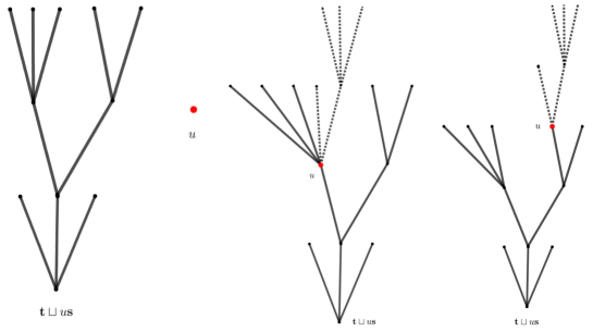
Figure 1. Example of the concatenation of t (solid lines) and s (dotted lines) at particle $u$ (red vertex). In the left hand-side picture, $u\notin\textbf{t}$. In the middle picture, $u\in\textbf{t}$ and $u$ is not a leaf. In the right hand-side picture, $u\in\textbf{t}$ and $u$ is a leaf.

Let $\textbf{t}\in\mathcal{T}$, a spine v is the genealogical line of a leaf $v\in\textbf{t}$, i.e. $\textbf{v}:=\llbracket\varnothing,v\rrbracket.$ The height of v is $|\textbf{v}|=|v|$. For $m\leq|\textbf{v}|$, we denote by $v^{(m)}$ the unique ancestor of $v$ with height $m$. Let us denote by

$$\mathcal{T}^{k}:=\{(\textbf{t};\textbf{v}_{1},\dots,\textbf{v}_{k}):\ \textbf{t}\ \mbox{is a tree and }\textbf{v}_{i}\mbox{ is a spine on }\textbf{t}\mbox{ for all }i\leq k\},$$

the set of trees with $k$ spines and by $\mathcal{T}^{k}_{n}:=\{(\textbf{t};\textbf{v}_{1},\dots,\textbf{v}_{k})\in\mathcal{T}^{k}:|\textbf{t}|=n\}$ its restriction to trees in $\mathcal{T}_{n}$. See Figure 2.

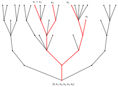
Figure 2. Example of a tree with 5 spines.

We observe that the spines are a special type of rooted trees, the trees with only one leaf. In other words, we can have the following operations: its restriction to the first $n$ generations $R_{n}(\textbf{v})$ and the subspine $S_{u}(\textbf{v})$ attached at some $u\in\mathcal{U}$. For a $(\textbf{t};\textbf{v}_{1},\dots,\textbf{v}_{k})\in\mathcal{T}^{k}$, we define its restriction to the first $n$- generations as follows

$$R_{n}(\textbf{t};\textbf{v}_{1},\dots,\textbf{v}_{k}):=(R_{n}(\textbf{t});R_{n}(\textbf{v}_{1}),\dots,R_{n}(\textbf{v}_{k}))\qquad n\geq 0.$$

Note that $R_{n}(\textbf{t};\textbf{v}_{1},\dots,\textbf{v}_{k})\in\mathcal{T}_{n}^{k}$. Let $(\textbf{t};\textbf{v}_{1},\dots,\textbf{v}_{k})\in\mathcal{T}^{k}$, and $u\in\textbf{t}$. We define the marks (or spines) of $u$ by

$$M_{u}(\textbf{t};\textbf{v}_{1},\dots,\textbf{v}_{k}):=\{\textbf{v}_{i}:u\in\textbf{v}_{i}\}.$$

If there is not confusion, we will only use the notation $M_{u}(\textbf{t})$. We note that $R_{|u|}(\textbf{v})=R_{|u|}(\textbf{w})$ for all $\textbf{v},\textbf{w}\in M_{u}(\textbf{t})$. We define the subtree and subspine attached at $u$ by

$$S_{u}(\textbf{t};\textbf{v}_{1},\dots,\textbf{v}_{k}):=(S_{u}(\textbf{t});S_{u}(\textbf{v}_{1}),\dots,S_{u}(\textbf{v}_{k})).$$

More precisely, $M_{u}(\textbf{t})=\hbox{\cmsy\char 59\relax}$, then $S_{u}(\textbf{t};\textbf{v}_{1},\dots,\textbf{v}_{k})=S_{u}(\textbf{t}).$ On the other hand, if $M_{u}(\textbf{t})=\{\textbf{v}_{i_{1}},\dots,\textbf{v}_{i_{m}}\}$, then $S_{u}(\textbf{t};\textbf{v}_{1},\dots,\textbf{v}_{k})=(S_{u}(\textbf{t});S_{u}(\textbf{v}_{i_{1}}),\dots,S_{u}(\textbf{v}_{i_{m}})).$

The concatenation of two spines $\textbf{v}=\llbracket\varnothing,v\rrbracket$ and $\textbf{w}=\llbracket\varnothing,w\rrbracket$ at $u$ can be performed for any $u,v,w\in\mathcal{U}$ but if $u\in\textbf{v}$ is not a leaf, then the result is a tree with two leaves $v$ and $uw$, not a spine. Thus, we restrict to concatenate spines only when $u\notin\textbf{v}$ or when $u\in\textbf{v}$ is a leaf (i.e. $u=v$). In these cases, we define the spine concatenation as

$$\textbf{v}\bigsqcup u\textbf{w}:=\left\{\begin{array}[]{ll}\llbracket\varnothing,v\rrbracket&\text{ if }u\notin\textbf{v},\\ \llbracket\varnothing,uw\rrbracket&\text{ if }u=v.\end{array}\right.$$

Finally, we define the concatenation of two trees with spines at a leaf. Let $(\textbf{t};\textbf{v}_{1},\dots,\textbf{v}_{k})\in\mathcal{T}^{k}$, $(\textbf{s};\textbf{w}_{1},\dots,\textbf{w}_{m})\in\mathcal{T}^{m}$ and $u\in\textbf{t}$ be a leaf such that $M_{u}(\textbf{t})=\{\textbf{v}_{i_{1}},\dots,\textbf{v}_{i_{m}}\}$. We define the concatenation of $(\textbf{t};\textbf{v}_{1},\dots,\textbf{v}_{k})$ and $(\textbf{s};\textbf{w}_{1},\dots,\textbf{v}_{m})$ at $u$ as

$$(\textbf{t};\textbf{v}_{1},\dots,\textbf{v}_{k})\bigsqcup u(\textbf{s};\textbf{w}_{1},\dots,\textbf{w}_{m}):=\left(\textbf{t}\bigsqcup u\textbf{s};\widetilde{\textbf{v}}_{1},\dots,\widetilde{\textbf{v}}_{k}\right),$$

where $\widetilde{\textbf{v}}_{i}=\textbf{v}_{i}$ if $\textbf{v}_{i}\notin M_{u}(\textbf{t})$ and $\widetilde{\textbf{v}}_{i_{j}}=\textbf{v}_{i_{j}}\sqcup u\textbf{w}_{j},$ for $\textbf{v}_{i_{j}}\in M_{u}(\textbf{t})$. We observe that $(\textbf{t};\textbf{v}_{1},\dots,\textbf{v}_{k})\bigsqcup u(\textbf{s};\textbf{w}_{1},\dots,\textbf{w}_{m})\in\mathcal{T}^{k}$, see for an illustrative example at Figure 3.

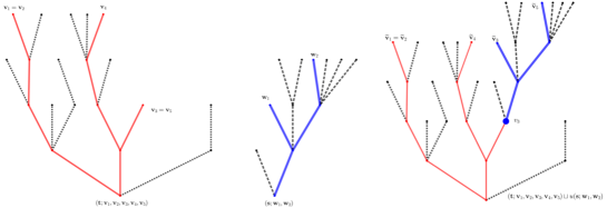
Figure 3. Example of the spine concatenation of $(\textbf{t};\textbf{v}_{1},\dots,\textbf{v}_{5})$ and $(\textbf{s};\textbf{w}_{1},\textbf{w}_{2})$ at leaf $v_{3}$.

2.2. Galton-Watson trees in varying environments with spines

In this subsection, we study probability measures in the set of rooted trees which describes the genealogies of Galton-Watson processes in varying environments. Such trees are known as Galton-Watson trees in varying environments (GWTVE). Recall that in a Galton-Watson process in an environment $e=(q_{1},q_{2},\ldots)$, any particle in generation $i$ gives birth to particles in generation $i+1$ according to the law $q_{i+1}$. Therefore, we say that $(\textbf{T},\mathbb{P}^{(e)})$ is a Galton-Watson tree in the environment $e$ whenever T is a $\mathcal{T}$-valued random variable under law $\mathbb{P}^{(e)}$ satisfying

$$\textbf{G}^{(e)}_{n}(\textbf{t}):=\mathbb{P}^{(e)}(R_{n}(\textbf{T})=R_{n}(\textbf{t}))=\prod_{u\in\textbf{t}:\,|u|<n}q_{|u|+1}(l_{u}(\textbf{t})),$$

for all $n\geq 0$  and all trees $\textbf{t}\in\mathcal{T}$.

Observe that the population size process $Z=(Z_{n}:n\geq 0)$ defined by $Z_{n}:=X_{n}(\textbf{T})$ is a Galton-Watson process in an environment $e$. In other words, $((X_{m}(\textbf{T}),m\leq n),\textbf{G}_{n}^{(e)})$ has the same law as $((Z_{m},m\leq n),\mathbb{P}^{(e)})$.

A tree in an environment $e$ with $k$ spines, under law $\mathbb{P}^{(e)}$, can be constructed as follows:

1. We start with one particle which carries $k$ marks.

2. Particles in generation $m$ gives birth to particles in generation $m+1$ according to $q_{m+1}$.

3. If a particle with $j$ marks gives birth to $a>0$ particles, then, the $j$ marks choose a particle to follow independently and uniformly at random from amongst the $a$ available.

4. If a particle with $j$ marks give birth to $0$ particles, then its marks are transferred to the graveyard $\Delta$.

With this construction in hand, we introduce a Galton-Watson tree in an environment $e$ with $k\geq 1$ spines. The tree with $k$-spines $(\textbf{T};\textbf{V}_{1},\ldots,\textbf{V}_{k})$ is a $\mathcal{T}^{k}$-valued r.v. with the following distribution

$$\begin{split}\mathbb{P}_{n}^{(e,k)}((\textbf{t};\textbf{v}_{1},\ldots,\textbf{v}_{k})):=&\ \mathbb{P}^{(e)}\left(R_{n}(\textbf{T};\textbf{V}_{1},\ldots,\textbf{V}_{k})=R_{n}(\textbf{t};\textbf{v}_{1},\ldots,\textbf{v}_{k})\right)\\ =&\prod_{u\in\textbf{t}:\,|u|<n}q_{|u|+1}(l_{u}(\textbf{t}))\prod_{i=1}^{k}\prod_{u\in\textbf{v}_{i}:\,|u|<|\textbf{v}_{i}|\wedge n}\frac{1}{l_{u}(\textbf{t})}\\ =&\prod_{i=1}^{k}\prod_{u\in\textbf{v}_{i}:\,|u|<|\textbf{v}_{i}|\wedge n}\frac{1}{l_{u}(\textbf{t})}\mathbf{G}_{n}^{(e)}(\textbf{t}),\end{split}$$

for any $n\geq 0$ and $(\textbf{t};\textbf{v}_{1},\ldots,\textbf{v}_{k})\in\mathcal{T}^{k}$. Observe from the above definition, that the first and second products follows from steps (iii) and (ii), respectively, from our construction of trees in an environment $e$. It is important to note that we can extend the definition to the case $k=0$, by just taking a Galton-Watson tree in environment $e$, that is

$$\mathbb{P}_{n}^{(e,0)}(\textbf{t}):=\mathbf{G}_{n}^{(e)}(\textbf{t}),\qquad\textbf{t}\in\mathcal{T}.$$

For an environment $e=(q_{1},q_{2},\dots)$ and $m\in\mathbb{N}_{0}$, we set the shift environment as

$$e_{m}:=(q_{m+1},q_{m+2},\dots).$$

Our first result, in this section, states that the law $\mathbb{P}_{n}^{(e,k)}$ satisfies a time-dependent Markov branching property, in that the descendants of any particle behave independently of the rest of the tree.

Proposition 1.

Markov property for GWTVE with spines under $\mathbb{P}_{n}^{(e,k)}$. Let $e$ be an environment and $(\textbf{T};\textbf{V}_{1},\ldots,\textbf{V}_{k})$ a r.v. taking values in $\mathcal{T}_{n}^{k}$ with distribution $\mathbb{P}_{n}^{(e,k)}$. Suppose that a particle $u\in\textbf{T}$ satisfies $|M_{u}(\textbf{T})|=j$ and $|u|=m$, for some $0\leq j\leq k$ and $0\leq m<n$. Then, $S_{u}(\textbf{T};\textbf{V}_{1},\ldots,\textbf{V}_{k})$ is independent of the rest of the system, that is, from the sigma-algebra

$$\sigma(\{R_{m}(\textbf{T};\textbf{V}_{1},\ldots,\textbf{V}_{k})\}\cup\{S_{w}(\textbf{T};\textbf{V}_{1},\ldots,\textbf{V}_{k}):w\in\textbf{T},|w|=m,w\neq u\}).$$

In addition, the law of $S_{u}(\textbf{T};\textbf{V}_{1},\ldots,\textbf{V}_{k})$ is given by $\mathbb{P}_{n-m}^{(e_{m},j)}$.

Proof.

Independence is clear since by construction all the subtrees with (possible zero) spines starting at generation $m$ are independent. On the other hand, the environment starting at generation $m$ is the shifted environment $e_{m}=(q_{m+1},q_{m+2},\dots)$ and from our hypotheses the subtree starting at $u$ has $j$ marks and $n-m$ generations. Therefore, the distribution of the subtree and spines starting at $u$ is clearly given by $\mathbb{P}_{n-m}^{(e_{m},j)}$ which implies our result. ∎

Let $k\geq 1$ and denote by

$$\widehat{\mathcal{T}}_{n}^{k}=\{(\textbf{t};\textbf{v}_{1},\dots,\textbf{v}_{k})\in\mathcal{T}^{k}_{n}:|\textbf{v}_{i}|=n\mbox{ and }\textbf{v}_{i}\neq\textbf{v}_{j}\mbox{ for all }1\leq i\neq j\leq k\}$$

the subspace of $\mathcal{T}^{k}_{n}$ where all spines are distinct and alive at time $n$. Now, we want to define a new probability measure by conditioning $((\textbf{T};\textbf{V}_{1},\ldots,\textbf{V}_{k}),\mathbb{P}_{n}^{(e,k)})$ to the subspace $\widehat{\mathcal{T}}_{n}^{k}$ in such a way that spines are choosing uniformly from all distinct particles alive at time $n$. Recall that $X_{n}(\textbf{t})=\#\{u\in\textbf{t}:|u|=n\}$ is the population size at the $n$-th generation of the tree t.

Let $\theta\in[0,1)$ and define the function $g_{n,\theta}:\mathcal{T}^{k}\rightarrow\mathbb{R}$, as follows

(7) $$g_{n,\theta}(\textbf{t};\textbf{v}_{1},\dots,\textbf{v}_{k}):=\mathbf{1}_{\{\textbf{v}_{i}\neq\textbf{v}_{j},i\neq j\}}\mathbf{1}_{\{|\textbf{v}_{i}|=n,i\leq k\}}e^{-\theta X_{n}(\textbf{t})}\prod_{i=1}^{k}\prod_{u\in\textbf{v}_{i}:\,|u|<n}l_{u}(\textbf{t}).$$

We also introduce the law $\mathbf{Q}_{n}^{(e,k,\theta)}$ by

(8) $$\begin{split}\mathbf{Q}_{n}^{(e,k,\theta)}((\textbf{t};\textbf{v}_{1},\ldots,\textbf{v}_{k})):=&\frac{g_{n,\theta}(\textbf{t};\textbf{v}_{1},\dots,\textbf{v}_{k})\mathbb{P}^{(e,k)}_{n}((\textbf{t};\textbf{v}_{1},\ldots,\textbf{v}_{k}))}{\mathbb{E}^{(e,k)}_{n}[g_{n,\theta}(\textbf{T};\textbf{V}_{1},\ldots,\textbf{V}_{k})]},\end{split}$$

for $(\textbf{t};\textbf{v}_{1},\dots,\textbf{v}_{k})\in\widehat{\mathcal{T}}^{k}_{n}$. Then we find the following result:

Proposition 2.

Let $((\textbf{T};\textbf{V}_{1},\ldots,\textbf{V}_{k}),\mathbb{P}^{(e,k)}_{n})$ be a Galton-Watson tree up to time $n$ with $k$ spines. Then,

$$\mathbb{E}^{(e,k)}_{n}[g_{n,\theta}(\textbf{T};\textbf{V}_{1},\ldots,\textbf{V}_{k})]=\mathbb{E}^{(e)}[Z_{n}(Z_{n}-1)\cdots(Z_{n}-k+1)e^{-\theta Z_{n}}].$$

In particular,

$$\mathbf{Q}_{n}^{(e,k,\theta)}((\textbf{t};\textbf{v}_{1},\ldots,\textbf{v}_{k}))=\frac{\mathbf{1}_{\{\textbf{v}_{i}\neq\textbf{v}_{j},i\neq j\}}\mathbf{1}_{\{|\textbf{v}_{i}|=n,i\leq k\}}e^{-\theta X_{n}(\textbf{t})}}{\mathbb{E}^{(e)}[Z_{n}(Z_{n}-1)\cdots(Z_{n}-k+1)e^{-\theta Z_{n}}]}\mathbf{G}_{n}^{(e)}(\textbf{t}).$$

Proposition 2 reveals that if the population size $Z_{n}$ has finite $k$-th moments then we do not need any discounting term and can simply take $\theta=0$ in the above definition. In such cases, we denote $\mathbf{Q}_{n}^{(e,k)}:=\mathbf{Q}_{n}^{(e,k,0)}$. However, in general the offspring distributions and population sizes need not have finite $k$-th moments, in which case we must take $\theta>0$. Importantly, the introduction of discounting in the change of measure turns out to be very natural. Crucially, it will allow our approach to work elegantly in generality, that is, without any additional moment assumptions or ad hoc truncations (as needed in [11]).

The new measure $\mathbf{Q}_{n}^{(e,k,\theta)}$ is defined via a change of measure relative to $\mathbb{P}^{(e,k)}_{n}$ only at time $n$. Of course, we could determine the martingale corresponding to this change of measure, $M_{n}=(M_{n}(m))_{m=0,\dots,n}$, by projecting $g_{n,\theta}(\textbf{T};\textbf{V}_{1},\ldots,\textbf{V}_{k})$ onto the natural filtration at times $m\in\{0,1,\dots,n\}$. However, for our purposes, we will not need to compute this martingale directly and instead calculate projections only for certain events related to properties of interest (e.g. to describe the first split of the spines in Proposition 6).

Proof of Proposition 2.

By definition of $\mathbb{P}^{(e,k)}$ and $g_{n,\theta}$, the second identity holds true as soon as we prove the first one. In addition, we also deduce

$$\mathbb{E}^{(e,k)}_{n}[g_{n,\theta}(\textbf{T};\textbf{V}_{1},\ldots,\textbf{V}_{k})]=\underset{(\textbf{t};\textbf{v}_{1},\dots,\textbf{v}_{k})\in\mathcal{T}^{k}_{n}}{\sum}\mathbf{1}_{\{\textbf{v}_{i}\neq\textbf{v}_{j},i\neq j\}}\mathbf{1}_{\{|\textbf{v}_{i}|=n,i\leq k\}}e^{-\theta X_{n}(\textbf{t})}\mathbf{G}_{n}^{(e)}(\textbf{t}).$$

For a fixed tree $\textbf{t}\in\mathcal{T}_{n}$, the term associated with $(\textbf{t};\textbf{v}_{1},\dots,\textbf{v}_{k})$ only contributes to the sum when all spines $(\textbf{v}_{1},\dots,\textbf{v}_{k})$ are different and have height equals $n$. In this case, it contributes with the value $e^{-\theta X_{n}(\textbf{t})}$. On the other hand, we observe that there are $X_{n}(\textbf{t})(X_{n}(\textbf{t})-1)\times\cdots\times(X_{n}(\textbf{t})-k+1)$ different possibilities to choose these $k$ spines from those particles alive at time $n$, i.e. $X_{n}(\textbf{t})$. Therefore,

(9) $$\begin{split}\underset{(\textbf{t};\textbf{v}_{1},\dots,\textbf{v}_{k})\in\mathcal{T}^{k}_{n}}{\sum}&e^{-\theta X_{n}(\textbf{t})}\mathbf{1}_{\{\textbf{v}_{i}\neq\textbf{v}_{j},i\neq j\}}\mathbf{1}_{\{|\textbf{v}_{i}|=n,i\leq k\}}\mathbf{G}_{n}^{(e)}(\textbf{t})\\ =&\underset{\textbf{t}\in\mathcal{T}_{n}}{\sum}e^{-\theta X_{n}(\textbf{t})}X_{n}(\textbf{t})(X_{n}(\textbf{t})-1)\times\cdots\times(X_{n}(\textbf{t})-k+1)\mathbf{G}_{n}^{(e)}(\textbf{t}).\end{split}$$

Since $\{(X_{m}(\textbf{T}),m\leq n),\textbf{G}_{n}^{(e)}\}$ has the same law as $\{(Z_{m},m\leq n),\mathbb{P}^{(e)}\}$, we clearly deduce the first identity in the statement. This completes the proof. ∎

From the construction of $\mathbf{Q}_{n}^{(e,k,\theta)}$, we see that $\mathbf{Q}_{n}^{(e,k,\theta)}(X_{n}(\textbf{t})\geq k)=1$. In other words, under $\mathbf{Q}_{n}^{(e,k,\theta)}$, there are at least $k$ different particles at generation $n$. Importantly, under $\mathbf{Q}_{n}^{(e,k,\theta)}$, the $k$ spines are a uniform choice without replacement from all particles alive at generation $n$. In addition, under $\mathbf{Q}_{n}^{(e,k,\theta)}$, the total population size at time $n$, $Z_{n}$ is the $k$-size biased and $\theta$-discounted transformation of its distribution under $\mathbb{P}^{(e)}$.

As before, we extend the definition of $\mathbf{Q}_{n}^{(e,k,\theta)}$ for $k=0$, by only performing the discounting. In other words, $g_{n,\theta}:\mathcal{T}\rightarrow\mathbb{R}$ is given by $g_{n,\theta}(\textbf{t}):=e^{-\theta X_{n}(\textbf{t})}$ and

$$\begin{split}\mathbf{Q}_{n}^{(e,0,\theta)}(\textbf{t}):=&\frac{e^{-\theta X_{n}(\textbf{t})}}{\mathbb{E}^{(e)}[e^{-\theta Z_{n}}]}\mathbf{G}_{n}^{(e)}(\textbf{t}).\end{split}$$

Our next results says that the Markov branching property given in Proposition 1 is inherited by the measure $\mathbf{Q}_{n}^{(e,k,\theta)}$. In particular, it implies that if we have two subtrees such that neither of their roots are part of the other subtree, then the subtrees are independent.

In order to simplify notation, for any random variable $X$, we denote by $X^{[k]}$ its $k$-th factorial, that is $X^{[k]}:=X(X-1)\times\cdots\times(X-k+1)$.

Proposition 3 (Markov property for GWTVE with spines under $\mathbf{Q}_{n}^{(e,k,\theta)}$.).

For $k\geq 1$, let $(\textbf{T};\textbf{V}_{1},\ldots,\textbf{V}_{k})$ be a $\mathcal{T}_{n}^{k}$-valued random variable with law $\mathbf{Q}_{n}^{(e,k,\theta)}$. Suppose that a particle $u\in\textbf{T}$ satisfies $|M_{u}(\textbf{T})|=j$ and $|u|=m$ for some $0\leq j\leq k$ and $0\leq m<n$ and let

$$\mathcal{G}:=\sigma(\{R_{m}(\textbf{T};\textbf{V}_{1},\ldots,\textbf{V}_{k})\}\cup\{S_{w}(\textbf{T};\textbf{V}_{1},\ldots,\textbf{V}_{k}):w\in\textbf{T},|w|=m,w\neq u\}).$$

Then, $S_{u}(\textbf{T};\textbf{V}_{1},\ldots,\textbf{V}_{k})$ is independent of $\mathcal{G}$ and its law is given by $\mathbf{Q}_{n-m}^{(e_{m},j,\theta)}$.

Proof.

We first treat the case $j\geq 1$. Let $(\textbf{s};\textbf{w}_{1},\dots,\textbf{w}_{j})\in\mathcal{T}_{n-m}^{j}$ and denote by $\mathcal{G}$ for the $\sigma$-algebra generated by the whole information of $(\textbf{T};\textbf{V}_{1},\ldots,\textbf{V}_{k})$ except for $S_{u}(\textbf{T};\textbf{V}_{1},\ldots,\textbf{V}_{k})$. By the conditioned version of the Radon Nikodym theorem (see [11, Lemma 13]), we have

(10) $$\begin{split}\mathbf{Q}_{n}^{(e,k,\theta)}&\left(S_{u}(\textbf{T};\textbf{V}_{1},\ldots,\textbf{V}_{k})=(\textbf{s};\textbf{w}_{1},\dots,\textbf{w}_{j})\mid\mathcal{G}\right)\\ &\hskip 56.9055pt=\frac{\mathbb{P}^{(e,k)}_{n}(g_{n,\theta}(\textbf{T};\textbf{V}_{1},\ldots,\textbf{V}_{k})\mathbf{1}_{S_{u}(\textbf{T};\textbf{V}_{1},\ldots,\textbf{V}_{k})=(\textbf{s};\textbf{w}_{1},\dots,\textbf{w}_{j})}\mid\mathcal{G})}{\mathbb{P}^{(e,k)}_{n}(g_{n,\theta}(\textbf{T};\textbf{V}_{1},\ldots,\textbf{V}_{k})\mid\mathcal{G})}.\end{split}$$

Let us enumerate by $u_{1},\dots,u_{X_{m}(\textbf{t})-1}$ the particles at generation $m$ which are different to $u$. Next, we observe that $(\textbf{T};\textbf{V}_{1},\ldots,\textbf{V}_{k})$ can be rewritten as the concatenation of its restriction to the $m$-th generation with the subtrees which are attached at each particles in generation $m$ (see Figure 4), that is

$$(\textbf{T};\textbf{V}_{1},\ldots,\textbf{V}_{k})=R_{m}(\textbf{T};\textbf{V}_{1},\ldots,\textbf{V}_{k})\bigsqcup uS_{u}(\textbf{T};\textbf{V}_{1},\ldots,\textbf{V}_{k})\underset{r=1}{\overset{X_{m}(\textbf{t})-1}{\bigsqcup}}u_{r}S_{u_{r}}(\textbf{T};\textbf{V}_{1},\ldots,\textbf{V}_{k}).$$

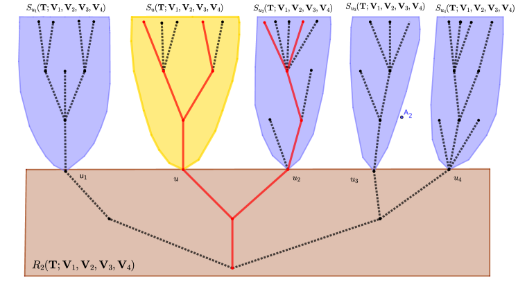
Figure 4. Decomposition of the tree with spines $(\textbf{T};\textbf{V}_{1},\textbf{V}_{2},\textbf{V}_{3},\textbf{V}_{4})$ at generation $m=2$ into its restriction up to generation $2$ concatenated with the subtrees attached to particles $u,u_{1},u_{2},u_{3}$ and $u_{4}$. Particles without marks have dotted lines. The spines are the solid red lines.

Therefore, we can decompose the population size at the $n$-th generation of the tree t as follows

$$X_{n}(\textbf{t})=X_{n-m}(S_{u}(\textbf{T}))+\sum_{r=1}^{X_{m}(\textbf{t})-1}X_{n-m}(S_{u_{r}}(\textbf{T})).$$

Denote by $I:=\{i\leq k:\textbf{V}_{i}\in M_{u}(\textbf{t})\}$. With the previous decompositions, we observe

$$g_{n,\theta}(\textbf{T};\textbf{V}_{1},\ldots,\textbf{V}_{k})=g_{n-m,\theta}(S_{u}(\textbf{T};\textbf{V}_{1},\ldots,\textbf{V}_{k}))h,$$

where $g_{n,\theta}$ is defined in (7) and

$$\begin{split}h&:=\prod_{r=1}^{X_{m}(\textbf{t})-1}e^{-\theta X_{n-m}(S_{u_{r}}(\textbf{T}))}\left(\prod_{i\in I}\prod_{w\in\textbf{V}_{i}:|w|<m}l_{w}(\textbf{T})\right)\\ &\hskip 113.81102pt\times\mathbf{1}_{\{\textbf{V}_{j}\neq\textbf{V}_{\ell},j\neq\ell\in I^{c}\}}\prod_{j\in I^{c}}\mathbf{1}_{\{|\textbf{V}_{j}|=n\}}\prod_{v\in\textbf{V}_{r}:|v|<n}l_{v}(\textbf{T}),\end{split}$$

which is an $\mathcal{G}$-measurable function. Now, we use equation (10) to obtain

$$\begin{split}&\mathbf{Q}_{n}^{(e,k,\theta)}\left(S_{u}(\textbf{T};\textbf{V}_{1},\ldots,\textbf{V}_{k})=(\textbf{s};\textbf{w}_{1},\dots,\textbf{w}_{j})\mid\mathcal{G}\right)\\ &\hskip 56.9055pt=\frac{\mathbb{P}^{(e,k)}_{n}(g_{n-m,\theta}(\textbf{S};\textbf{W}_{1},\ldots,\textbf{W}_{j})h\mathbf{1}_{(\textbf{S};\textbf{W}_{1},\ldots,\textbf{W}_{j})=(\textbf{s};\textbf{w}_{1},\dots,\textbf{w}_{j})}\mid\mathcal{G})}{\mathbb{P}^{(e,k)}_{n}(g_{n-m,\theta}(S_{u}(\textbf{T};\textbf{V}_{1},\ldots,\textbf{V}_{k}))h\mid\mathcal{G})}\\ &\hskip 56.9055pt=\frac{\mathbb{P}^{(e_{m},j)}_{n-m}(g_{n-m,\theta}(\textbf{S};\textbf{W}_{1},\ldots,\textbf{W}_{j})\mathbf{1}_{(\textbf{S};\textbf{W}_{1},\ldots,\textbf{W}_{j})=(\textbf{s};\textbf{w}_{1},\dots,\textbf{w}_{j})})}{\mathbb{P}^{(e_{m},j)}_{n-m}(g_{n-m,\theta}(\textbf{S};\textbf{W}_{1},\ldots,\textbf{W}_{j}))}\\ &\hskip 56.9055pt=\mathbf{Q}_{n-m}^{(e_{m},j,\theta)}\left(\textbf{s};\textbf{w}_{1},\dots,\textbf{w}_{j}\right),\end{split}$$

where in the second identity we have used that $h$ is $\mathcal{G}$ measurable and in the last identity we used Proposition 1. For the case $j=0$, we follow the same arguments. Indeed, we only require to change $\textbf{s}\in\mathcal{T}_{n-m}$ at the beginning, take $\textbf{S}:=S_{u}(\textbf{T};\textbf{V}_{1},\ldots,\textbf{V}_{k})$ in the middle and note that an empty product is equal to one. ∎

Now, our aim is to provide a construction, forward in time, of the tree under $\mathbf{Q}_{n}^{(e,k,\theta)}$. Our construction follows from a recursive procedure. For the cases $k=1$ and $\theta=0$, such construction can be found in [16, Section 1.4] and for the case $k=2$ and $\theta=0$, see [6, Section 2].

Let $g\in\{1,\dots,k\}$ be the number of spine groups created at a given time and let $k_{1},\ldots,k_{g}\geq 1$ be their sizes. Denote by $g_{r}$ the number of groups of size $r$. By a combinatorial argument we have

$$\underset{i=1}{\overset{g}{\sum}}k_{i}=k,\qquad\underset{r=1}{\overset{k}{\sum}}\ g_{r}=g\qquad\mbox{and}\qquad\underset{r=1}{\overset{k}{\sum}}\ rg_{r}=k.$$

We also introduce the first time that the spines split apart and the last time all the spines are together by $\hat{\psi}_{1}$ and $\psi_{1}$, respectively. We observe that $\hat{\psi}_{1}=\psi_{1}+1$. We often swap between using $\psi_{1}$ and $\hat{\psi}_{1}$ as most appropriate. For simplicity of exposition, for $g\geq 2$ and $k=k_{1}+\dots+k_{g}$, we denote

(11) $$C_{k;k_{1},\dots,k_{g}}:=\{\mbox{Spines split from a group of size $k$ into }g\mbox{ groups of sizes }k_{1},\dots,k_{g}\}.$$

Proposition 4 (A $k$-spine construction under $\mathbf{Q}_{n}^{(e,k,\theta)}$).

A tree with $k\geq 1$ different spines up to generation $n$, under $\mathbf{Q}_{n}^{(e,k,\theta)}$, is constructed as follows.

1. We start with a particle with $k$ marks.

2. If $k=1$, we consider $\psi_{1}=n$. Otherwise, select $\psi_{1}$, the number of spine groups $g$ and their sizes $k_{1},\dots,k_{g}$ according to

   (12) $$\begin{split}\mathbf{Q}^{(e,k,\theta)}_{n}&\left(\psi_{1}=m,C_{k;k_{1},\dots,k_{g}}\right)\\ &=\frac{k!\Big{(}\left.\tfrac{\partial^{g}}{\partial s^{g}}f_{m+1}(s)\right|_{s=f_{m+1,n}(e^{-\theta})}\Big{)}\mathbb{E}^{(e)}\left[e^{-\theta Z_{n}}Z_{n}\right]\underset{i=1}{\overset{g}{\prod}}\mathbb{E}^{(e_{m+1})}\left[e^{-\theta Z_{n-m-1}}Z_{n-m-1}^{[k_{i}]}\right]}{\left(\underset{r=1}{\overset{k}{\prod}}g_{r}!\right)\left(\underset{i=1}{\overset{g}{\prod}}k_{i}!\right)\mathbb{E}^{(e)}\left[e^{-\theta Z_{n}}Z_{n}^{[k]}\right]\mathbb{E}^{(e_{m})}\left[e^{-\theta Z_{n-m}}Z_{n-m}\right]},\end{split}$$

   where $m\in\{0,\dots,n-1\}$, $g\in\{2,\dots,k\}$, $k_{1},\ldots,k_{g}\geq 1$ satisfying $k_{1}+\cdots+k_{g}=k$ and $g_{r}$ is the number of groups of size $r$.

3. An unmarked particle in generation $m\in\{0,\dots,n-1\}$ gives birth to unmarked particles in generation $m+1$, independently of other particles, with probability

   $$q_{m+1}^{(0,\theta)}\left(\ell\right):=q_{m+1}(\ell)\frac{f_{m+1,n}(e^{-\theta})^{\ell}}{\mathbb{E}^{(e_{m})}\left[e^{-\theta Z_{n-m}}\right]},\qquad\ell\geq 0.$$

4. A marked particle in generation $m\in\{0,\dots,\psi_{1}-1\}$ gives birth to particles in generation $m+1$ accordingly to

   $$\begin{split}&q_{m+1}^{(1,\theta)}\left(\ell\right):=\frac{\ell q_{m+1}(\ell)\left(f_{m+1,n}(e^{-\theta})\right)^{\ell-1}}{f_{m+1}^{\prime}(f_{m+1,n}(e^{-\theta}))},\qquad\ell\geq 1.\end{split}$$

   Uniformly, select one of the particles to carry the $k$ marks. All the other particles remain unmarked.

5. The marked particle at generation $m=\psi_{1}<n$ gives birth accordingly to

   $$q_{m+1}^{(g,\theta)}\left(\ell\right):=\ell^{[g]}q_{m+1}(\ell)\frac{(f_{m+1,n}(e^{-\theta}))^{l-g}}{\left.\tfrac{\partial^{g}}{\partial s^{g}}f_{m+1}(s)\right|_{s=f_{m+1,n}(e^{-\theta})}},\qquad\ell\geq g.$$

   Uniformly, select $g$ of these particles as marked in generation $m+1$ with $k_{1},\dots,k_{g}$ marks, respectively. All the other particles remain unmarked.

6. Repeat steps (1)-(5) for each of the $g$ marked particles. Next, we have to construct $g$ independent trees with $k_{1},\dots,k_{g}$ different spines under the measure $\mathbf{Q}^{(e_{m+1},k_{j},\theta)}_{n-m-1}$, respectively.

The proof of the above construction follows directly from Proposition 3 (which is step (6)) and the forthcoming Propositions 5 and 6.

It is important to note that whenever the process possesses finite $k$-th moments, we can take $\theta=0$. In this case, the distribution of $\psi_{1}$ and the spine subgroups can be simplified, $q_{m+1}^{(0,0)}=q_{m+1}$, $q_{m+1}^{(1,0)}$ is the $q_{m+1}$ size-biased transformation of $q_{m+1}$ and $q_{m+1}^{(g,0)}$ is the $q^{[g]}_{m+1}$  size-biased transform of $q_{m+1}$. This guarantees that at $m\neq\psi_{1}$ the marked particle has at least one child, and at $m=\psi_{1}$ the marked particle has at least $g$ children. If the process does not have finite $k$-th moments, then necessarily $\theta>0$. In this scenario the previous comment also holds.

Before we proceed with the proof of the construction of the tree under $\mathbf{Q}_{n}^{(e,k,\theta)}$, we compute the distribution of the total population size of unmarked particles who are descendants of the unmarked offspring of spine particles. More precisely, let $u$ be a spine particle and denote by $Y_{n}(u)$ the total population size of unmarked particles at generation $n$ that descend from the unmarked offspring of $u$, see Figure 5 for an illustrative example. In other words, if $u$ has $g$ marked children labelled by $uv_{1},\dots,uv_{g}$, then

$$Y_{n}(u):=X_{n-|u|}(S_{u}(\textbf{T}))-\sum_{j=1}^{g}X_{n-|uv_{j}|}(S_{uv_{j}}(\textbf{T})).$$

By Proposition 3, the variables $Y_{n}(u)$, for $u$ in the spines, are independent.

Lemma 1.

Let $(\textbf{T};\textbf{V}_{1},\dots,\textbf{V}_{k})$ be a tree with $k\geq 1$ spines, under $\mathbf{Q}_{n}^{(e,k,\theta)}$. For each $m\leq n-1$, let $u$ be a marked particle at generation $m$ whose offspring distribution is given by $q_{m+1}^{(g,\theta)}$, for $g\geq 1$. Then,

$$\mathbf{Q}_{n}^{(e,k,\theta)}\left[e^{-(\lambda-\theta)Y_{n}(u)}\right]=\frac{\left.\tfrac{\partial^{g}}{\partial s^{g}}f_{m+1}(s)\right|_{s=f_{m+1,n}(e^{-\lambda})}}{\left.\tfrac{\partial^{g}}{\partial s^{g}}f_{m+1}(s)\right|_{s=f_{m+1,n}(e^{-\theta})}},\qquad\lambda>0.$$

In particular, for $k=1$ we have

$$\mathbf{Q}_{n}^{(e,1,\theta)}\left[e^{-(\lambda-\theta)Z_{n}}\right]=\frac{e^{-\lambda}}{e^{-\theta}}\prod_{m=0}^{n-1}\frac{f_{m+1}^{\prime}(f_{m+1,n}(e^{-\lambda}))}{f_{m+1}^{\prime}(f_{m+1,n}(e^{-\theta}))},\qquad\lambda>0.$$

Proof.

From Proposition 3 and the definition of $\mathbf{Q}^{(e,0,\theta)}$, the descendants at generation $n$ of an unmarked particle at generation $m+1$ is given by

$$\mathbf{Q}_{n-m-1}^{(e_{m+1},0,\theta)}\left[e^{-(\lambda-\theta)Z_{n-m-1}}\right]=\frac{\mathbb{E}^{(e_{m+1})}\left[e^{-\lambda Z_{n-{m+1}}}\right]}{\mathbb{E}^{(e_{m+1})}\left[e^{-\theta Z_{n-{m+1}}}\right]}=\frac{f_{m+1,n}(e^{-\lambda})}{f_{m+1,n}(e^{-\theta})},\qquad\lambda>0.$$

If the particle $u$ has offspring distribution $q_{m+1}^{g,\theta}(\cdot)$, we know that it gives birth at least to $g$ market particles. Thus, by only considering all subtrees attached to unmarked offspring (which are independent), for $\lambda>0$, we get

$$\begin{split}\mathbf{Q}_{n}^{(e,k,\theta)}\left[e^{-(\lambda-\theta)Y_{n}(u)}\right]&=\underset{\ell=g}{\overset{\infty}{\sum}}\frac{\ell^{[g]}q_{m+1}(\ell)(f_{m+1,n}(e^{-\theta}))^{l-g}}{\left.\tfrac{\partial^{g}}{\partial s^{g}}f_{m+1}(s)\right|_{s=f_{m+1,n}(e^{-\theta})}}\frac{(f_{m+1,n}(e^{-\lambda}))^{l-g}}{(f_{m+1,n}(e^{-\theta}))^{l-g}}\\ &=\frac{\left.\tfrac{\partial^{g}}{\partial s^{g}}f_{m+1}(s)\right|_{s=f_{m+1,n}(e^{-\lambda})}}{\left.\tfrac{\partial^{g}}{\partial s^{g}}f_{m+1}(s)\right|_{s=f_{m+1,n}(e^{-\theta})}}.\end{split}$$

The second equality holds by independence and the decomposition

$$Z_{n}=1+\sum_{m=0}^{n-1}Y_{n}(v^{(m)}),$$

where $v^{(m)}$ is the particle at the spine with height $m$. ∎

Now, we proceed with Propositions 5 and 6 that will imply the construction of the tree under $\mathbf{Q}_{n}^{(e,k,\theta)}$. In order to do so, let us first recall some notation. Recall that $(f_{1},f_{2},\dots)$ denote the generating functions associated to the environment $e=(q_{1},q_{2},\dots).$ For each $0\leq m<n$ and $s\in[0,1]$, we define

$$f_{m,n}(s):=[f_{m+1}\circ\cdots\circ f_{n}](s),$$

and $f_{n,n}(s):=s$, where $f\circ g$ is the composition of $f$ with $g$. According to the monograph of Kersting and Vatutin [16], we have

(13) $$\mathbb{E}^{(e)}\left[s^{Z_{n}}\mid Z_{m}=1\right]=\mathbb{E}^{(e_{m})}\left[s^{Z_{n-m}}\right]=f_{m,n}(s)\qquad 0\leq m<n\quad\mbox{ and }\quad s\in[0,1].$$

In particular, for any $m\geq 0$

(14) $$\left\{(Z_{n+m},n\geq 0),\mathbb{P}^{(e)}(\ \cdot\mid Z_{m}=1)\right\}\overset{(d)}{=}\left\{(Z_{n},n\geq 0),\mathbb{P}^{(e_{m})}\right\},$$

and, for any $k\geq 1$, $0\leq m\leq n$ and $\theta\geq 0$,

(15) $$\mathbb{E}^{(e_{m})}\left[e^{-\theta Z_{n-m}}Z_{n-m}^{[k]}\right]=\mathbb{E}^{(e)}\left[e^{-\theta Z_{n}}Z_{n}^{[k]}\mid Z_{m}=1\right]=e^{-\theta k}\left.\frac{\partial^{k}}{\partial s^{k}}f_{m,n}(s)\right|_{s=e^{-\theta}}.$$

We also recall that $\psi_{1}$ and $\hat{\psi}_{1}$ denote the last time where all marks (or spines) are together and the first spine splitting time, respectively. In other words, if $\textbf{V}_{1},\dots,\textbf{V}_{k}$ denotes the spines, then

$$\{\psi_{1}=m\}=\{R_{m}(\textbf{V}_{1})=R_{m}(\textbf{V}_{i}),\forall i\leq k\}\bigcap\{\exists i\neq j:R_{m+1}(\textbf{V}_{i})\neq R_{m+1}(\textbf{V}_{j})\}.$$

Observe that, unlike the continuous time case $\psi_{1}$ and $\hat{\psi}_{1}$ are different, indeed $\hat{\psi}_{1}=\psi_{1}+1$ and $\hat{\psi}_{1}$ is a stopping time in the natural filtration of the branching process whereas $\psi_{1}$ is not.

The next result provides the distribution of $\psi_{1}$, hence implicitly that of $\hat{\psi}_{1}$. Observe that since we have finite second moment, when $k=2$ we may take $\theta=0$ and use the notation $\mathbf{Q}^{(e,2)}$. In this particular case, the next result explains the choice of the distribution of $\psi_{1}$ in the two spine decomposition in Cardona and Palau [6] which satisfies

(16) $$\mathbf{Q}_{n}^{(e,2)}(\psi_{1}=m)=\frac{\nu_{m+1}}{\mu_{m}}\left(\sum_{k=0}^{n-1}\frac{\nu_{k+1}}{\mu_{k}}\right)^{-1},\qquad 0\leq m\leq n-1.$$

Proposition 5.

Let $0\leq m<n$, then

$$\begin{split}\mathbf{Q}^{(e,k,\theta)}_{n}(\psi_{1}\geq m)&=\frac{\mathbb{E}^{(e)}\left[e^{-\theta Z_{n}}Z_{n}\right]}{\mathbb{E}^{(e)}\left[e^{-\theta Z_{n}}Z_{n}^{[k]}\right]}\frac{\mathbb{E}^{(e_{m})}\left[e^{-\theta Z_{n-m}}Z_{n-m}^{[k]}\right]}{\mathbb{E}^{(e_{m})}\left[e^{-\theta Z_{n-m}}Z_{n-m}\right]}.\end{split}$$

In particular, $\mathbf{Q}_{n}^{(e,2)}(\psi_{1}=m)$ has distribution (16).

Proof.

Observe that $\{\psi_{1}\geq m\}=\{R_{m}(\textbf{v}_{1})=R_{m}(\textbf{v}_{i}),i\leq k\}$ is the event that all $k$ spines are still together at time $m$. From Proposition 2, we have

$$\begin{split}\mathbf{Q}_{n}^{(e,k,\theta)}(\psi_{1}\geq m)=\frac{\underset{(\textbf{t};\textbf{v}_{1},\dots,\textbf{v}_{k})\in\mathcal{T}^{k}_{n}}{\sum}e^{-\theta X_{n}(\textbf{t})}\mathbf{1}_{\{R_{m}(\textbf{v}_{1})=R_{m}(\textbf{v}_{i}),i\leq k\}}\mathbf{1}_{\{\textbf{v}_{i}\neq\textbf{v}_{j},i\neq j\}}\mathbf{1}_{\{|\textbf{v}_{i}|=n,i\leq k\}}\mathbf{G}^{(e)}_{n}(\textbf{t})}{\mathbb{E}^{(e)}\left[e^{-\theta Z_{n}}Z_{n}^{[k]}\right]},\end{split}$$

Let $(\textbf{t};\textbf{v}_{1},\dots,\textbf{v}_{k})\in\mathcal{T}^{k}_{n}$ such that

$$\mathbf{1}_{\{R_{m}(\textbf{v}_{1})=R_{m}(\textbf{v}_{i}),i\leq k\}}\mathbf{1}_{\{\textbf{v}_{i}\neq\textbf{v}_{j},i\neq j\}}\mathbf{1}_{\{|\textbf{v}_{i}|=n,i\leq k\}}\neq 0.$$

We also let $u^{*}$ be the ancestor of $\textbf{v}_{1}$ at generation $m$. Then, $|M_{u^{*}}(\textbf{t})|=k$ . We enumerate by $u_{1},\dots,u_{X_{m}(\textbf{t})-1}$ the particles at generation $m$ which are different of $u^{*}$. As in the proof of the previous proposition, we decompose $(\textbf{t};\textbf{v}_{1},\ldots,\textbf{v}_{k})$ as the concatenation of its restriction to generation $m$ with all the subtrees which are attached to particles $u^{*},u_{1},\dots,u_{X_{m}(\textbf{t})-1}$ at generation $m$ (see for instance Figure 4), that is

(17) $$(\textbf{t};\textbf{v}_{1},\ldots,\textbf{v}_{k})=R_{m}(\textbf{t};\textbf{v}_{1},\ldots,\textbf{v}_{k})\underset{r=1}{\overset{X_{m}(\textbf{t})-1}{\bigsqcup}}u_{r}S_{u_{r}}(\textbf{t};\textbf{v}_{1},\ldots,\textbf{v}_{k})\bigsqcup u^{*}S_{u^{*}}(\textbf{t};\textbf{v}_{1},\ldots,\textbf{v}_{k}).$$

Since $|M_{u^{*}}(\textbf{t})|=k$, we have $S_{u^{*}}(\textbf{t};\textbf{v}_{1},\ldots,\textbf{v}_{k})=(\textbf{t}^{\ast};\textbf{v}_{1}^{\ast},\dots,\textbf{v}_{k}^{\ast})\in\mathcal{T}_{n-m}^{k}$. Moreover, we introduce $\textbf{t}_{r}:=S_{u_{r}}(\textbf{t};\textbf{v}_{1},\ldots,\textbf{v}_{k})$ which is clearly in $\mathcal{T}_{n-m}$ from our assumption. Additionally, we have $R_{m}(\textbf{t};\textbf{v}_{1},\ldots,\textbf{v}_{k})=(\textbf{s};\textbf{w}_{1},\dots,\textbf{w}_{k})\in\mathcal{T}_{m}^{k}$ and satisfies $X_{m}(\textbf{t})=X_{m}(\textbf{s})$. Thus, we can decompose $X_{n}(\textbf{t})$ as follows

(18) $$X_{n}(\textbf{t})=X_{n-m}(\textbf{t}^{\ast})+\sum_{j=1}^{X_{m}(\textbf{t})-1}X_{n-m}(\textbf{t}_{j}).$$

Then, by taking into account the environment and the previous decompositions, we have

$$\begin{split}&\underset{(\textbf{t};\textbf{v}_{1},\dots,\textbf{v}_{k})\in\mathcal{T}^{k}_{n}}{\sum}e^{-\theta X_{n}(\textbf{t})}\mathbf{1}_{\{R_{m}(\textbf{v}_{1})=R_{m}(\textbf{v}_{i}),i\leq k\}}\mathbf{1}_{\{\textbf{v}_{i}\neq\textbf{v}_{j},i\neq j\}}\mathbf{1}_{\{|\textbf{v}_{i}|=n,i\leq k\}}\mathbf{G}^{(e)}_{n}(\textbf{t})\\ &=\underset{(\textbf{s};\textbf{w}_{1},\dots,\textbf{w}_{k})\in\mathcal{T}^{k}_{m}}{\sum}\mathbf{1}_{\{\textbf{w}_{1}=\textbf{w}_{i},i\leq k\}}\mathbf{1}_{\{|\textbf{w}_{1}|=m\}}\prod_{r=1}^{X_{m}(\textbf{s})-1}\left(\underset{\textbf{t}_{r}\in\mathcal{T}_{n-m}}{\sum}e^{-\theta X_{n-m}(\textbf{t}_{r})}\mathbf{G}_{n-m}^{(e_{m})}(\textbf{t}_{r})\right)\mathbf{G}_{m}^{(e)}(\textbf{s})\\ &\hskip 85.35826pt\times\left(\underset{(\textbf{t}^{\ast};\textbf{v}_{1}^{\ast},\dots,\textbf{v}_{k}^{\ast})\in\mathcal{T}_{n-m}^{k}}{\sum}e^{-\theta X_{n-m}(\textbf{t}^{\ast})}\mathbf{1}_{\{\textbf{v}_{i}^{\ast}\neq\textbf{v}_{j}^{\ast},i\neq j\}}\mathbf{1}_{\{|\textbf{v}_{i}^{\ast}|=n-m,i\leq k\}}\mathbf{G}_{n-m}^{(e_{m})}(\textbf{t}^{\ast})\right).\end{split}$$

By equation (9), we deduce

$$\underset{(\textbf{t}^{\ast};\textbf{v}_{1}^{\ast},\dots,\textbf{v}_{k}^{\ast})\in\mathcal{T}_{n-m}^{k}}{\sum}e^{-\theta X_{n-m}(\textbf{t}^{\ast})}\mathbf{1}_{\{\textbf{v}_{i}^{\ast}\neq\textbf{v}_{j}^{\ast},i\neq j\}}\mathbf{1}_{\{|\textbf{v}_{i}^{\ast}|=n-m,i\leq k\}}\mathbf{G}_{n-m}^{(e_{m})}(\textbf{t}^{\ast})=\mathbb{E}^{(e_{m})}\left[e^{-\theta Z_{n-m}}Z_{n-m}^{[k]}\right].$$

On the other hand, for each $r\leq X_{m}(\textbf{s})-1$, we have

(19) $$\underset{\textbf{t}_{r}\in\mathcal{T}_{n-m}}{\sum}e^{-\theta X_{n-m}(\textbf{t}_{r})}\mathbf{G}_{n-m}^{(e_{m})}(\textbf{t}_{r})=\mathbb{E}^{(e_{m})}\left[e^{-\theta Z_{n-m}}\right]=f_{m,n}(e^{-\theta}),$$

and observe that for every tree s, there are $X_{m}(\textbf{s})$ possibilities to choose $\textbf{w}_{1}=\cdots=\textbf{w}_{k}$. Therefore,

$$\begin{split}\underset{(\textbf{s};\textbf{w}_{1},\dots,\textbf{w}_{k})\in\mathcal{T}^{k}_{m}}{\sum}&\mathbf{1}_{\{\textbf{w}_{1}=\textbf{w}_{i},i\leq k\}}\mathbf{1}_{\{|\textbf{w}_{1}|=m\}}\prod_{r=1}^{X_{m}(\textbf{s})-1}\left(\underset{\textbf{t}_{r}\in\mathcal{T}_{n-m}}{\sum}e^{-\theta X_{n-m}(\textbf{t}_{r})}\mathbf{G}_{n-m}^{(e_{m})}(\textbf{t}_{r})\right)\mathbf{G}_{m}^{(e)}(\textbf{s})\\ &\hskip 56.9055pt=\underset{\textbf{s}\in\mathcal{T}_{m}}{\sum}X_{m}(\textbf{s})\left(f_{m,n}(e^{-\theta})\right)^{X_{m}(\textbf{s})-1}\mathbf{G}_{m}^{(e)}(\textbf{s}).\end{split}$$

Putting all pieces together, we obtain

$$\mathbf{Q}^{(e,k,\theta)}_{n}(\psi_{1}\geq m)=\mathbb{E}^{(e)}[Z_{m}(f_{m,n}(e^{-\theta}))^{Z_{m}-1}]\frac{\mathbb{E}^{(e_{m})}\left[e^{-\theta Z_{n-m}}Z_{n-m}^{[k]}\right]}{\mathbb{E}^{(e)}\left[e^{-\theta Z_{n}}Z_{n}^{[k]}\right]}.$$

In order to get our result, we differentiate (13) and then deduce

(20) $$\begin{split}\mathbb{E}^{(e)}[Z_{m}(f_{m,n}(e^{-\theta}))^{Z_{m}-1}]&=f_{0,m}^{\prime}(f_{m,n}(e^{-\theta}))=\frac{f_{0,n}^{\prime}(e^{-\theta})}{f_{m,n}^{\prime}(e^{-\theta})}=\frac{\mathbb{E}^{(e)}\left[e^{-\theta Z_{n}}Z_{n}\right]}{\mathbb{E}^{(e_{m})}\left[e^{-\theta Z_{n-m}}Z_{n-m}\right]},\end{split}$$

where we have use that $f_{0,n}$ is a composition of functions and the chain rule for its derivative. The latter equality implies the first identity in the statement.

Finally, we compute the case when $k=2$. Recall that in this cases, we can take $\theta=0$. Hence from (1) and the shifted environment property (14), we see

$$\begin{split}\mathbf{Q}^{(e,2)}_{n}(\psi_{1}\geq m)&=\mathbb{E}^{(e)}[Z_{m}]\frac{\mathbb{E}^{(e_{m})}[Z_{n-m}(Z_{n-m}-1)]}{\mathbb{E}^{(e)}[Z_{n}(Z_{n}-1)]}\\ &=\mu_{m}\frac{\left(\frac{\mu_{n}}{\mu_{m}}\right)^{2}\underset{j=m}{\overset{n-1}{\sum}}\frac{\nu_{j+1}}{\mu_{j}}\mu_{m}}{\mu_{n}^{2}\underset{j=0}{\overset{n-1}{\sum}}\frac{\nu_{j+1}}{\mu_{j}}}=\frac{\underset{j=m}{\overset{n-1}{\sum}}\frac{\nu_{j+1}}{\mu_{j}}}{\underset{j=0}{\overset{n-1}{\sum}}\frac{\nu_{j+1}}{\mu_{j}}},\end{split}$$

which clearly implies that $\mathbf{Q}_{n}^{(e,2)}(\psi_{1}=m)$ has distribution (16). This finishes the proof. ∎

It is important to note that by an analogous technique, we can obtain the offspring distribution of particles off spines under $\mathbf{Q}_{n}^{(e,k,\theta)}$. More precisely, let $u$ be a particle without marks such that $|u|=m$. From Proposition 1, we see that under $\mathbf{Q}_{n}^{(e,k,\theta)}$, the subtree attached to $u$ has law $\mathbf{Q}_{n-m}^{(e,0,\theta)}$. Similarly to the proof of the previous proposition, we perform a decomposition by using all the subtrees attached to the offspring of $u$ and using equation (19), we deduce

(21) $$\mathbf{Q}_{n}^{(e,k,\theta)}(l_{u}=\ell)=q_{m+1}(\ell)\frac{f_{m+1,n}(e^{-\theta})^{\ell}}{\mathbb{E}^{(e_{m})}\left[e^{-\theta Z_{n-m}}\right]}.$$

From the change of measure (8), it is clear that under $\mathbf{Q}^{(e,k,\theta)}_{n}$, there are $k$ different spines at generation $n$. The latter can also be deduced from the forward construction. Indeed by a recursive argument, it is enough to show that if $\psi_{1}=n-1$, then $g=k$. Thus, by using Proposition 5 and (12), we may deduce

$$\mathbf{Q}^{(e,k,\theta)}_{n}\left(g=k\mid\psi_{1}=n-1\right)=\frac{e^{-k\theta}\left.\tfrac{\partial^{k}}{\partial s^{k}}f_{n}(s)\right|_{s=f_{n,n}(e^{-\theta})}}{\mathbb{E}^{(e_{n-1})}\left[e^{-\theta Z_{1}}Z_{1}^{[k]}\right]}.$$

Since $f_{n,n}(e^{-\theta})=e^{-\theta}$, the claim then follows from (15).

Now, we turn our attention into the offspring distribution of particles with marks under $\mathbf{Q}_{n}^{(e,k,\theta)}$. Suppose that at generation $m$ there is only one particle with $k$ marks, i.e. $R_{m}(\textbf{V}_{1})=R_{m}(\textbf{V}_{i})$ for each $i\leq k$. When this particle has offspring, the marks follows one or several of its offspring, i.e., the marks may split into different groups. Recall that $g\in\{1,\dots,k\}$ denotes the number of spine groups which are created at time $m+1$ and that $k_{1},\ldots,k_{g}\geq 1$ are their sizes. We also recall that $g_{r}$ denotes the number of groups of size $r$ and moreover that all those quantities satisfy

$$\underset{i=1}{\overset{g}{\sum}}k_{i}=k,\qquad\underset{r=1}{\overset{k}{\sum}}\ g_{r}=g\qquad\mbox{and}\qquad\underset{r=1}{\overset{k}{\sum}}\ rg_{r}=k.$$

Observe that under the event $\{\psi_{1}=m\}$, we necessarily have $g\geq 2$. Also, recall that $\hat{\psi}_{1}$ is the first time the spines split apart, $\psi_{1}$ is the last time all the spines are together, and $\hat{\psi}_{1}=\psi_{1}+1$. We often swap between using $\psi_{1}$ and $\hat{\psi}_{1}$ as most appropriate.

Proposition 6.

The probability that at generation $m$ the $k$ spines are still all together but at the next generation the spines have split into $g\in\{2,\dots,k\}$ groups of sizes $k_{1},\ldots,k_{g}\geq 1$ is given by (12), i.e.

$$\begin{split}&\mathbf{Q}^{(e,k,\theta)}_{n}\left(\psi_{1}=m,C_{k;k_{1},\dots,k_{g}}\right)\\ &=\frac{k!\Big{(}\left.\tfrac{\partial^{g}}{\partial s^{g}}f_{m+1}(s)\right|_{s=f_{m+1,n}(e^{-\theta})}\Big{)}\mathbb{E}^{(e)}\left[e^{-\theta Z_{n}}Z_{n}\right]\underset{i=1}{\overset{g}{\prod}}\mathbb{E}^{(e_{m+1})}\left[e^{-\theta Z_{n-m-1}}Z_{n-m-1}^{[k_{i}]}\right]}{\left(\underset{r=1}{\overset{k}{\prod}}g_{r}!\right)\left(\underset{i=1}{\overset{g}{\prod}}k_{i}!\right)\mathbb{E}^{(e)}\left[e^{-\theta Z_{n}}Z_{n}^{[k]}\right]\mathbb{E}^{(e_{m})}\left[e^{-\theta Z_{n-m}}Z_{n-m}\right]},\end{split}$$

where $C_{k;k_{1},\dots,k_{g}}$ is defined in (11).

Moreover, we may extend (12) to include the case when all $k$ spines remain together at generation $m+1$ (corresponding to $g=1$ and $k_{1}=k$) and additionally specify the offspring distribution of $V^{(m)}_{1}$. Indeed, suppose that the spines have not split by time $m$ and at generation $m+1$ the spines follow $g\in\{1,\dots,k\}$ groups of sizes $k_{1},\ldots,k_{g}\geq 1$, then, for $\ell\geq g$, we have

(22) $$\begin{split}\mathbf{Q}^{(e,k,\theta)}_{n}&\left(\hat{\psi}_{1}>m;\,\,l_{V^{(m)}_{1}}=\ell;\mbox{ at time $m+1$ the spines follow }g\mbox{ groups of sizes }k_{1},\dots,k_{g}\right)\\ &=\frac{q_{m+1}(\ell)\ell!k!\left(f_{m+1,n}(e^{-\theta})\right)^{\ell-g}}{(\ell-g)!\left(\underset{r=1}{\overset{k}{\prod}}g_{r}!\right)\left(\underset{i=1}{\overset{g}{\prod}}k_{i}!\right)}\frac{\mathbb{E}^{(e)}\left[e^{-\theta Z_{n}}Z_{n}\right]\underset{i=1}{\overset{g}{\prod}}\mathbb{E}^{(e_{m+1})}\left[e^{-\theta Z_{n-m-1}}Z_{n-m-1}^{[k_{i}]}\right]}{\mathbb{E}^{(e)}\left[e^{-\theta Z_{n}}Z_{n}^{[k]}\right]\mathbb{E}^{(e_{m})}\left[e^{-\theta Z_{n-m}}Z_{n-m}\right]}.\end{split}$$

In particular, if $g=1$ we find that, given all the spines stay together, the offspring distribution is (once) size biased and discounted according to population size over the remaining time, as follows:

(23) $$\begin{split}&\mathbf{Q}^{(e,k,\theta)}_{n}\left(l_{V^{(m)}_{1}}=\ell\mid\psi_{1}>m\right)=\frac{\ell q_{m+1}(\ell)\left(f_{m+1,n}(e^{-\theta})\right)^{\ell-1}}{f_{m+1}^{\prime}(f_{m+1,n}(e^{-\theta}))}.\end{split}$$

Proof.

We first prove identity (22). In order to do so, we use the same tree decomposition as in the proof Proposition 5. Indeed, under the event

$$\{m\leq\psi_{1}\}\cap\{l_{v^{(m)}_{1}}=\ell\}\cap\{\mbox{the spines follow }g\mbox{ groups of sizes }k_{1},\dots,k_{g}\},$$

we decompose $(\textbf{t};\textbf{v}_{1},\dots,\textbf{v}_{k})\in\mathcal{T}^{k}_{n}$ into (see (17)),

$$(\textbf{t};\textbf{v}_{1},\ldots,\textbf{v}_{k})=(\textbf{s};\textbf{w}_{1},\dots,\textbf{w}_{k})\underset{r=1}{\overset{X_{m}(\textbf{t})-1}{\bigsqcup}}u_{r}\textbf{t}_{r}\bigsqcup u^{*}(\textbf{t}^{\ast};\textbf{v}_{1}^{\ast},\dots,\textbf{v}_{k}^{\ast})$$

where $u^{*}$ is the ancestor of $\textbf{v}_{1}$ at generation $m$, the other particles at generation $m$ are labeled by $u_{1},\dots,u_{X_{m}(\textbf{t})-1}$; the subtrees $(\textbf{s};\textbf{w}_{1},\dots,\textbf{w}_{k})=R_{m}(\textbf{t};\textbf{v}_{1},\ldots,\textbf{v}_{k})\in\mathcal{T}_{m}^{k}$, $\textbf{t}_{r}=S_{u_{r}}(\textbf{t};\textbf{v}_{1},\ldots,\textbf{v}_{k})\in\mathcal{T}_{n-m}$ and $(\textbf{t}^{\ast};\textbf{v}_{1}^{\ast},\dots,\textbf{v}_{k}^{\ast})=S_{u^{*}}(\textbf{t};\textbf{v}_{1},\ldots,\textbf{v}_{k})\in\mathcal{T}_{n-m}^{k}$.

Next, we observe that a similar decomposition for $(\textbf{t}^{\ast};\textbf{v}_{1}^{\ast},\dots,\textbf{v}_{k}^{\ast})$ can be given at generation $m+1$. By hypothesis, $u^{*}$ has $\ell-g$ offspring without marks and $g$ with marks. We label by $y_{1},\dots,y_{\ell-g}$ the offspring without marks and by $y_{1}^{*},\dots,y_{g}^{*}$ those with $k_{1},\dots,k_{g}$ marks, respectively. We denote by $\textbf{r}_{i}:=S_{y_{i}}(\textbf{t}^{\ast};\textbf{v}_{1}^{\ast},\dots,\textbf{v}_{k}^{\ast})\in\mathcal{T}_{n-m-1}$, for $i\leq\ell-g$, and $(\textbf{t}^{\ast,j};\textbf{v}_{1}^{\ast,j},\dots,\textbf{v}_{k_{j}}^{\ast,j}):=S_{y_{j}^{*}}(\textbf{t}^{\ast};\textbf{v}_{1}^{\ast},\dots,\textbf{v}_{k}^{\ast})\in\mathcal{T}_{n-m-1}^{k_{j}}$ for all $j\leq g$. Then, the following decomposition holds

(24) $$(\textbf{t}^{\ast};\textbf{v}_{1}^{\ast},\dots,\textbf{v}_{k}^{\ast})=(\textbf{s}^{*};\textbf{w}_{1}^{*},\dots,\textbf{w}_{k}^{*})\ \underset{i=1}{\overset{\ell-g}{\bigsqcup}}\ y_{i}\textbf{r}_{i}\ \underset{j=1}{\overset{g}{\bigsqcup}}\ y_{j}^{*}(\textbf{t}^{\ast,j};\textbf{v}_{1}^{\ast,j},\dots,\textbf{v}_{k_{i}}^{\ast,j}),$$

where $(\textbf{s}^{*};\textbf{w}_{1}^{*},\dots,\textbf{w}_{k}^{*}):=R_{1}(\textbf{t}^{\ast};\textbf{v}_{1}^{\ast},\dots,\textbf{v}_{k}^{\ast})\in\mathcal{T}_{1}^{k}$ and has $\ell$ leaves where $\ell-g$ has no marks and the remaining $g$ leaves has $k_{1},\dots,k_{g}$ marks. Moreover, we can decompose $X_{n-m}(\textbf{t}^{\ast})$ as follows

(25) $$X_{n-m}(\textbf{t}^{\ast})=\sum_{i=1}^{\ell-g}X_{n-m-1}(\textbf{r}_{i})+\sum_{j=1}^{g}X_{n-m-1}(\textbf{t}^{\ast,j}).$$

For simplicity on exposition, we let

$$A:=\mathbf{Q}^{(e,k,\theta)}_{n}\left(\hat{\psi}_{1}>m;\,\,l_{V^{(m)}_{1}}=\ell;\mbox{ at $m+1$ the spines follow }g\mbox{ groups of sizes }k_{1},\dots,k_{g}\right).$$

We proceed similarly as in the proof of the previous proposition, that is by Proposition 2 and taking into account the environment in decompositions (17), (18), (24) and (25), we deduce

$$\begin{split}A&\mathbb{E}^{(e)}\left[e^{-\theta Z_{n}}Z_{n}^{[k]}\right]\\ &=\underset{(\textbf{s};\textbf{w}_{1},\dots,\textbf{w}_{k})\in\mathcal{T}^{k}_{m}}{\sum}\mathbf{1}_{\{\textbf{w}_{1}=\textbf{w}_{i},i\leq k\}}\mathbf{1}_{\{|\textbf{w}_{1}|=m\}}\prod_{r=1}^{X_{m}(\textbf{s})-1}\left(\underset{\textbf{t}_{r}\in\mathcal{T}_{n-m}}{\sum}e^{-\theta X_{n-m}(\textbf{t}_{r})}\mathbf{G}_{n-m}^{(e_{m})}(\textbf{t}_{r})\right)\mathbf{G}_{m}^{(e)}(\textbf{s})\\ &\hskip 14.22636pt\times q_{m+1}(\ell)\mathbf{1}_{\{\mbox{g children has }k_{1},\dots,k_{g}\mbox{ marks}\}}\prod_{i=1}^{\ell-g}\left(\underset{\textbf{r}_{i}\in\mathcal{T}_{n-m-1}}{\sum}e^{-\theta X_{n-m-1}(\textbf{r}_{i})}\mathbf{G}_{n-m-1}^{(e_{m+1})}(\textbf{r}_{i})\right)\\ &\hskip 14.22636pt\times\underset{j=1}{\overset{g}{\prod}}\underset{(\textbf{t}^{\ast,j};\textbf{v}_{1}^{\ast,j},\dots,\textbf{v}_{k_{j}}^{\ast,j})\in T_{n-m-1}^{\,k_{j}}}{\sum}\mathbf{1}_{\{\textbf{v}_{l}^{\ast,j}\neq\textbf{v}_{s}^{\ast,j},l\neq s\}}\mathbf{1}_{\{|\textbf{v}_{l}^{\ast,j}|=n-m-1,l\leq k_{j}\}}e^{-\theta X_{n-m-1}(\textbf{t}^{\ast,j})}\mathbf{G}_{n-m-1}^{(e_{m+1})}(\textbf{t}^{\ast,j}).\end{split}$$

Observe that there are $X_{m}(\textbf{s})$ possibilities to choose $\textbf{w}_{1}$, $u^{*}$ has $\ell$ offspring with probability $q_{m+1}(\ell)$, from these offspring there are ${\ell\choose g}$ possibilities to select $g$ of them with marks, there are $g!/\underset{r=1}{\overset{k}{\prod}}g_{r}!$ ways of arranging the values $k_{1},\ldots,k_{g}$ with the sizes of each group and $k!/\underset{i=1}{\overset{g}{\prod}}k_{i}!$ ways to arrange the $k$ spines into $g$ groups of sizes $k_{1},\ldots,k_{g}$. Thus using (19) for every $r\leq X_{m}(\textbf{s})-1$ and every $i\leq\ell-g$; and (9) for every $j\leq g$, we obtain

$$A=\mathbb{E}^{(e)}[Z_{m}(f_{m,n}(e^{-\theta}))^{Z_{m}-1}]\frac{q_{m+1}(\ell)\ell!k!\left(f_{m+1,n}(e^{-\theta})\right)^{\ell-g}}{(\ell-g)!\left(\underset{r=1}{\overset{k}{\prod}}g_{r}!\right)\left(\underset{i=1}{\overset{g}{\prod}}k_{i}!\right)}\frac{\underset{i=1}{\overset{g}{\prod}}\mathbb{E}^{(e_{m+1})}\left[e^{-\theta Z_{n-m-1}}Z_{n-m-1}^{[k_{i}]}\right]}{\mathbb{E}^{(e)}\left[e^{-\theta Z_{n}}Z_{n}^{[k]}\right]},$$

which implies (22) after using (20).

For identity (23), we take $g=1$ in (22) and use Proposition 5 with $m+1$ instead of $m$ to obtain

$$\begin{split}&\mathbf{Q}^{(e,k,\theta)}_{n}\left(\psi_{1}>m,l_{V^{(m)}_{1}}=\ell\right)\\ &=\ell q_{m+1}(\ell)\left(f_{m+1,n}(e^{-\theta})\right)^{\ell-1}\frac{\mathbb{E}^{(e_{m+1})}\left[e^{-\theta Z_{n-m-1}}Z_{n-m-1}\right]}{\mathbb{E}^{(e_{m})}\left[e^{-\theta Z_{n-m}}Z_{n-m}\right]}\mathbf{Q}^{(e,k,\theta)}_{n}(\psi_{1}\geq m+1).\end{split}$$

By (20) we have

$$\begin{split}\frac{\mathbb{E}^{(e_{m+1})}\left[e^{-\theta Z_{n-m-1}}Z_{n-m-1}\right]}{\mathbb{E}^{(e_{m})}\left[e^{-\theta Z_{n-m}}Z_{n-m}\right]}=\frac{f_{m+1,n}^{\prime}(e^{-\theta})}{f_{m,n}^{\prime}(e^{-\theta})}=\frac{1}{f_{m+1}^{\prime}(f_{m+1,n}(e^{-\theta}))},\end{split}$$

where we have use that $f_{m,n}$ is a composition of functions and the chain rule for its derivative. By observing that $\{\psi_{1}\geq m+1\}=\{\psi_{1}>m\}$ and performing conditional probability, we get (23).

Finally, we prove (12). So let $g\geq 2$. In this case, $\{m\leq\psi_{1}\}=\{m=\psi_{1}\}$ and by summing over all possible values of $\ell$ and using the $g$-th derivative of the Laplace transform, we obtain (12). This completes the proof. ∎

3. Scaling limits of critical GWVE trees

The proof of our main result (Theorem 1) requires several preliminary results that are presented in this section. Most of them are limiting behaviours of functionals of trees with $k$ spines, under $\mathbf{Q}_{n}^{(e,k,\theta)}$, and of the total population size under the original probability measure but conditional on survival. In order to do so, we first introduce some notation. Recall that $\psi_{1}$ denotes the first time that a second spine is created. Hence for $1\leq i\leq k-1$, we introduce recursively $\psi_{i}$, the last time where there are at most $i$ marked particles, as follows

$$\psi_{i}=\max\{m\geq 0:\mbox{ at generation }m\mbox{ there are at most }i\mbox{ marked particles}\}.$$

Additionally, we denote by $\hat{\psi}_{i}=\psi_{i}+1$, the $i$-th spine split time (although note these split times may coincide, for example, the first and second spine split times may be equal which corresponds to marks following three different particles).

We also introduce

$$A_{n,m}:=\frac{a^{(e_{m+1})}_{n-(m+1)}}{a_{n}^{(e)}}=1-\sum_{j=0}^{m}\frac{\nu_{j+1}}{\mu_{j}}\left(\sum_{k=0}^{n-1}\frac{\nu_{k+1}}{\mu_{k}}\right)^{-1},\qquad\mbox{ for }0\leq m<n.$$

Note that $\{A_{n,m}:m=0,\dots,n-1\}\subset[0,1]$ is a decreasing sequence with $A_{n,n-1}=0$. If we define $A_{n,-1}:=1$, we can introduce a partition of $[0,1]$ as follows

$$R^{(n)}=\{0=A_{n,n-1}<A_{n,n-2}<\ldots<A_{n,0}<A_{n,-1}\}.$$

From the proof of [6, Lemma 3] (see last equation), one can deduce that under condition ($\filledstar$), the norm of the previous partition is such that

(26) $$\underset{n\rightarrow\infty}{\lim}||R^{(n)}||=\underset{n\rightarrow\infty}{\lim}\max_{0\leq m\leq n-1}\left\{\frac{\nu_{m+1}}{\mu_{m}}\left(\sum_{k=0}^{n-1}\frac{\nu_{k+1}}{\mu_{k}}\right)^{-1}\right\}=0.$$

Indeed according to the proof of [6, Lemma 3], the previous uniform convergence only requires that the following condition holds (see inequality (25) in [6]): there exists $c>0$ such that

$$f^{\prime\prime}_{k}\leq cf^{\prime}_{k}(1)(1+f_{k}^{\prime}(1)),\qquad\textrm{for all}\quad k\geq 1,$$

which actually is fulfilled under our condition ($\filledstar$) by taking $\epsilon=1/2$, see for instance inequality (6) in Kersting [14].

Next, we denote by

$$\rho_{0}=0,\quad\mbox{and}\qquad\rho_{n}=\frac{\mathbb{E}^{(e)}[Z_{n}(Z_{n}-1)]}{\mathbb{E}^{(e)}[Z_{n}]^{2}}=\sum_{k=0}^{n-1}\frac{\nu_{k+1}}{\mu_{k}},\qquad n\geq 1.$$

Since $A_{n,-1}=1$, we have

(27) $$\frac{\rho_{m}}{\rho_{n}}=1-A_{n,m-1},\qquad 0\leq m\leq n,$$

which describes an increasing sequence that can be thought as a cumulative probability distribution. We can thus define its right-continuous generalised inverse as

$$\tau_{n}(t)=\max\{k\geq 0:\rho_{k}\leq t\rho_{n}\},\qquad t\in[0,1].$$

Moreover, the norm of $(\rho_{m}/\rho_{n};0\leq m\leq n)$ is equal to the norm of the partition $R^{(n)}$. Then, by (26), the following convergence is uniform on $0\leq t\leq 1$

(28) $$1-A_{n,\tau_{n}(t)-1}=\frac{\rho_{\tau_{n}(t)}}{\rho_{n}}\longrightarrow t,\qquad\text{ as }n\rightarrow\infty.$$

Recall that $(f_{1},f_{2},\dots)$ denote the generating functions associated to the environment $e=(q_{1},q_{2},\dots).$ For every $f_{k}$, we define its shape function, $\varphi_{k}:[0,1)\rightarrow\infty$, as

$$\varphi_{k}(s):=\frac{1}{1-f_{k}(s)}-\frac{1}{f_{k}^{\prime}(1)(1-s)},\qquad 0\leq s<1.$$

The function $\varphi_{k}$ can be extend continuously to $s=1$, by writing $\varphi_{k}(1)=\nu_{k}/2$. Recall that $f_{m,n}=f_{m+1}\circ\ldots\circ f_{n}$. According to [14, Lemma 5], for every $0\leq m<n$,

(29) $$\frac{1}{1-f_{m,n}(s)}=\frac{\mu_{m}}{\mu_{n}(1-s)}+\mu_{m}\underset{k=m+1}{\overset{n}{\sum}}\frac{\varphi_{k}(f_{k,n}(s))}{\mu_{k-1}},\qquad 0\leq s<1.$$

In addition, by performing a small modification in the proof of Lemma 8 in [14], we have

(30) $$\underset{0\leq s\leq 1}{\sup}\left|\underset{k=m+1}{\overset{n}{\sum}}\frac{\varphi_{k}(f_{k,n}(s))}{\mu_{k-1}}-\frac{\rho_{n}-\rho_{m}}{2}\right|=o\left(\frac{\rho_{n}}{2}\right),$$

uniformly for all $m<n$. Moreover, for any $0<T<1$, Kersting showed in [15, equation (5)] that

(31) $$\underset{k=m+1}{\overset{n}{\sum}}\frac{\varphi_{k}(f_{k,n}(0))}{\mu_{k-1}}=\frac{\rho_{n}-\rho_{m}}{2}(1+o(1)),$$

uniformly for all $m$ such that $\rho_{m}\leq T\rho_{n}$. With all these ingredients in hand, we proceed to prove the following limiting result.

Proposition 7.

Assume that condition ($\filledstar$) is satisfied. Let $0<T<1$ and $u_{n}:[0,1]\rightarrow\{0,1,\dots,n\}$ be a sequence of functions such that $\rho_{u_{n}(t)}/\rho_{n}\rightarrow\varrho(t)$, uniformly, for $0\leq t\leq T$, as $n\rightarrow\infty$, where $\varrho:[0,1]\rightarrow[0,1]$ is a (non-decreasing) function satisfying $\varrho(t)<1$, for all $t<1$. Then,

$$\left(\left(a_{n-u_{n}(t)}^{(e_{u_{n}(t)})}\right)^{-1}Z_{n-u_{n}(t)}\ ;\ \mathbb{P}^{(e_{u_{n}(t)})}(\ \cdot\ |Z_{n-u_{n}(t)}>0)\right)\stackrel{{\scriptstyle(d)}}{{\longrightarrow}}\left(\mathbf{e};\mathbb{P}\right),\qquad\mbox{ as }\ n\rightarrow\infty,$$

uniformly for every $t\leq T$, where $\mathbf{e}$ is a standard exponential r.v., under $\mathbb{P}$, and “$\stackrel{{\scriptstyle(d)}}{{\longrightarrow}}$” means convergence in distribution.

Proof.

Let $0<T<1$. We observe that in order to get our result, it is enough to prove that for every $\lambda>0$, the following limit holds

$$\underset{n\rightarrow\infty}{\lim}\,\,\underset{0\leq t\leq T}{\sup}\mathbb{E}^{(e_{u_{n}(t)})}\left[\left.1-e^{-\lambda\left(a_{n-u_{n}(t)}^{(e_{u_{n}(t)})}\right)^{-1}Z_{n-u_{n}(t)}}\right|Z_{n-u_{n}(t)}>0\right]=\frac{\lambda}{1+\lambda}.$$

In order to prove our claim, we let $m<n$ such that $\rho_{m}<\varrho(T)\rho_{n}$. By (29), we have

$$\begin{split}\mathbb{E}^{(e_{m})}&\left[\left.1-e^{-\lambda\left(a_{n-m}^{(e_{m})}\right)^{-1}Z_{n-m}}\right|Z_{n-m}>0\right]=\frac{1-f_{m,n}\left(e^{-\lambda/a_{n-m}^{(e_{m})}}\right)}{1-f_{m,n}(0)}\\ &=\left(\frac{1}{\mu_{n}}+\underset{k=m+1}{\overset{n}{\sum}}\frac{\varphi_{k}(f_{k,n}(0))}{\mu_{k-1}}\right)\left(\frac{1}{\mu_{n}\left(1-e^{-\lambda/a_{n-m}^{(e_{m})}}\right)}+\underset{k=m+1}{\overset{n}{\sum}}\frac{\varphi_{k}\left(f_{k,n}\left(e^{-\lambda/a_{n-m}^{(e_{m})}}\right)\right)}{\mu_{k-1}}\right)^{-1}.\end{split}$$

We observe that for every $m$ with $\rho_{m}\leq\varrho(T)\rho_{n}$, the following inequality is satisfied

$$\frac{1}{a_{n-m}^{(e_{m})}}=\frac{1}{a_{n}^{(e)}}\frac{\rho_{n}}{\rho_{n}-\rho_{m}}\leq\frac{1}{a_{n}^{(e)}}\frac{1}{1-\varrho(T)}.$$

Then,

(32) $$\left(1-e^{-\lambda/a_{n-m}^{(e_{m})}}\right)=\frac{\lambda}{a_{n}^{(e)}}\frac{\rho_{n}}{\rho_{n}-\rho_{m}}(1+o(1)),$$

uniformly for all $m$ such that $\rho_{m}\leq\varrho(T)\rho_{n}$. Recall that $a_{n}^{(e)}=\mu_{n}\rho_{n}/2$ and by criticality $\mu_{n}^{-1}=o(\rho_{n})$. Then using (30), (31) and (32), we get

$$\begin{split}\mathbb{E}^{(e_{m})}&\left[\left.1-e^{\lambda\left(a_{n-m}^{(e_{m})}\right)^{-1}Z_{n-m}}\right|Z_{n-m}>0\right]\\ &=\left(o(1)+\frac{\rho_{n}-\rho_{m}}{2\rho_{n}}(1+o(1))\right)\left(\frac{\rho_{n}-\rho_{m}}{2\rho_{n}\lambda}+\frac{\rho_{n}-\rho_{m}}{2\rho_{n}}+o(1)\right)^{-1}.\end{split}$$

uniformly for all $m$ such that $\rho_{m}\leq\varrho(T)\rho_{n}$. By hypothesis, $\rho_{u_{n}(t)}/\rho_{n}\rightarrow\varrho(t)$ uniformly for $0\leq t\leq T$. Then, we conclude

$$\mathbb{E}^{(e_{u_{n}(t)})}\left[\left.1-e^{-\lambda\left(a_{n-u_{n}(t)}^{(e_{u_{n}(t)})}\right)^{-1}Z_{n-u_{n}(t)}}\right|Z_{n-u_{n}(t)}>0\right]\underset{n\rightarrow\infty}{\longrightarrow}\frac{1-\varrho(t)}{\lambda^{-1}(1-\varrho(t))+(1-\varrho(t))}=\frac{\lambda}{1+\lambda}$$

uniformly for every $t\leq T$, as expected. ∎

For a given $\theta$, we define $\theta_{n}:=\theta/a_{n}^{(e)}$. To simplify the notation, for every $0\leq m<n$ and $k\in\mathbb{N}$, we introduce

(33) $$F_{k,n,m}:=\frac{\mathbb{E}^{(e_{m})}\left[e^{-\theta_{n}Z_{n-m}}Z_{n-m}^{[k]}\right](1+\theta A_{n,m-1})^{k+1}\mu_{m}}{\left(a_{n}^{(e)}\right)^{k-1}k!(A_{n,m-1})^{k-1}\mu_{n}}.$$

As an application, we have the following lemma.

Lemma 2.

Let $0<T<1$. Suppose that $Z$ is a regular critical GWVE or equivalently that condition ($\filledstar$) is satisfied, and $u_{n}:[0,1]\rightarrow\{0,1,\dots,n\}$ is a sequence of functions such that $\rho_{u_{n}(t)}/\rho_{n}\rightarrow\varrho(t)$, uniformly, for $0\leq t\leq T$, as $n\rightarrow\infty$, where $\varrho:[0,1]\rightarrow[0,1]$ is a (non-decreasing) function satisfying that $\varrho(t)<1$, for all $t<1$. Then,

$$\lim_{n\rightarrow\infty}F_{k_{i},n,u_{n}(t)}=1,$$

uniformly on $0\leq t\leq T$ and $k_{i}\leq k.$

Proof.

For a fixed $k$, we can rewrite $F_{k,n,m}$ as follows

$$\mathbb{E}^{(e_{m})}\left[\left.e^{-\theta_{n}Z_{n-m}}\frac{Z_{n-m}^{[k]}}{\left(a_{n}^{(e)}\right)^{k}}\right|Z_{n-m}>0\right]\frac{(1+\theta A_{n,m-1})^{k+1}}{(A_{n,m-1})^{k}}\frac{a_{n}^{(e)}A_{n,m-1}\mathbb{P}^{(e_{m})}(Z_{n-m}>0)\mu_{m}}{\mu_{n}}.$$

From our hypothesis and (27), $A_{n,u_{n}(t)-1}$ converges to $1-\varrho(t)$, as $n\rightarrow\infty$, uniformly on $0\leq t\leq T$. Then, by the previous result and the continuous mapping Theorem [13, Theorem 5.27], we have

$$\left(A_{n,u_{n}(t)-1}\left(a_{n-u_{n}(t)}^{(e_{u_{n}(t)})}\right)^{-1}Z_{n-u_{n}(t)}\ ;\ \mathbb{P}^{(e_{u_{n}(t)})}(\ \cdot\ |Z_{n-u_{n}(t)}>0)\right)\stackrel{{\scriptstyle(d)}}{{\longrightarrow}}\left((1-\varrho(t))\mathbf{e};\mathbb{P}\right).$$

where $\mathbf{e}$ is an exponential r.v., under $\mathbb{P}$. Note that $A_{n,u_{n}(t)-1}\left(a_{n-u_{n}(t)}^{(e_{u_{n}(t)})}\right)^{-1}=\left(a_{n}^{(e)}\right)^{-1}$ converges to zero as $n$ goes to infinity. Since $f(x)=e^{-\theta x}x^{k_{i}}$ is a bounded function, we have

(34) $$\mathbb{E}^{(e_{u_{n}(t)})}\left[\left.e^{-\theta Z_{n-u_{n}(t)}/a_{n}^{(e)}}\frac{Z_{n-u_{n}(t)}^{[k]}}{\left(a_{n}^{(e)}\right)^{k}}\right|Z_{n-u_{n}(t)}>0\right]\longrightarrow\mathbb{E}\left[e^{-\theta(1-\varrho(t))Y}(1-\varrho(t))^{k}\mathbf{e}^{k}\right],$$

uniformly on $0\leq t\leq T$. On the other hand, it is known that

$$\mathbb{E}\left[e^{-\theta(1-\varrho(t))\mathbf{e}}(1-\varrho(t))^{k}\mathbf{e}^{k}\right]=\frac{(1-\varrho(t))^{k}}{(1+\theta(1-\varrho(t)))^{k+1}}=\underset{n\rightarrow\infty}{\lim}\frac{(A_{n,u_{n}(t)-1})^{k}}{(1+\theta A_{n,u_{n}(t)-1})^{k+1}},$$

uniformly on $[0,T]$. Then, by applying the behaviour of the survival probability, the result holds for every fixed $k$. Since we have a finite quantity of $k_{i}\leq k$, the uniform convergence on all possible values of $k_{i}$ also holds true. ∎

Similar arguments allow us to prove the following lemma.

Lemma 3.

Let $0<T<1$ and $\lambda>0$. Suppose that $Z$ is a regular critical GWVE. We also consider $u_{n}:[0,1]\rightarrow\{0,1,\dots,n\}$, a sequence of functions such that $\rho_{u_{n}(t)}/\rho_{n}\rightarrow\varrho(t)$, uniformly, for $0\leq t\leq T$, as $n\rightarrow\infty$, where $\varrho:[0,1]\rightarrow[0,1]$ is a (non-decreasing) function such that $\varrho(t)<1$, for all $t<1$. Then,

$$\begin{split}\underset{n\rightarrow\infty}{\lim}\mathbf{Q}^{(e_{u_{n}(t)},k_{i},\theta_{n})}_{n-u_{n}(t)}\left[e^{-(\lambda-\theta)Z_{n-u_{n}(t)}/a_{n}^{e}}\right]=&\frac{(1+\theta(1-\varrho(t)))^{k_{i}+1}}{(1+\lambda(1-\varrho(t)))^{k_{i}+1}},\end{split}$$

uniformly on $0\leq t\leq T$ and $k_{i}\leq k.$

Proof.

By definition of $\mathbf{Q}^{(e_{u_{n}(t)},k,\theta_{n})}_{n-u_{n}(t)}$, we have

$$\begin{split}\mathbf{Q}^{(e_{u_{n}(t)},k,\theta_{n})}_{n-u_{n}(t)}\left[e^{-(\lambda-\theta)Z_{n-u_{n}(t)}/a_{n}^{e}}\right]&=\frac{\mathbb{E}^{(e_{u_{n}(t)})}\left[e^{-\lambda Z_{n-u_{n}(t)}/a_{n}^{(e)}}Z_{n-u_{n}(t)}^{[k]}\right]}{\mathbb{E}^{(e_{u_{n}(t)})}\left[e^{-\theta Z_{n-u_{n}(t)/a_{n}^{(e)}}}Z_{n-u_{n}(t)}^{[k]}\right]}\\ &=\frac{\mathbb{E}^{(e_{u_{n}(t)})}\left[\left.e^{-\lambda Z_{n-u_{n}(t)}/a_{n}^{(e)}}Z_{n-u_{n}(t)}^{[k]}\right|Z_{n-u_{n}(t)}>0\right]}{\mathbb{E}^{(e_{u_{n}(t)})}\left[\left.e^{-\theta Z_{n-u_{n}(t)/a_{n}^{(e)}}}Z_{n-u_{n}(t)}^{[k]}\right|Z_{n-u_{n}(t)}>0\right]}.\end{split}$$

The result then follows from the asymptotic in (34). ∎

Recall that $\hat{\psi}_{1}$ and $\psi_{1}$ denote the first time the spines split apart and the last time all the spines are together, respectively, and that $\hat{\psi}_{1}=\psi_{1}+1$. Now, we compute the limiting distribution of $\psi_{1}$ under $\mathbf{Q}^{(e_{\cdot},k,\theta_{n})}_{n-\cdot}$, as $n\rightarrow\infty$, and show that asymptotically, the first split is binary and that the number of marks following each of those spines is uniformly distributed on $1,\dots,k$. Moreover, we also deduce that the first spine splitting time and the sizes of the subgroups are asymptotically independent.

We also recall from (11) the definition of $C_{k;k_{1},\dots,k_{g}}$ for $g\geq 2$ and $\{k_{i},i\geq g\}$ satisfying $k_{1}+\cdots+k_{g}=k$.

Proposition 8.

Assume that condition ($\filledstar$) is satisfied and let $0\leq T<1$. Consider $u_{n}:[0,1]\rightarrow\{0,1,\dots,n\}$, a sequence of functions such that $\rho_{u_{n}(r)}/\rho_{n}\rightarrow\varrho(r)$, uniformly, for $0\leq r\leq T$, as $n\rightarrow\infty$, where $\varrho:[0,1]\rightarrow[0,1]$ is a (non-decreasing) function such that $\varrho(r)<1$, for all $r<1$. Let $k_{1}$ and $k_{2}$ such that $k_{1}+k_{2}=k$. Then, uniformly on $0\leq\varrho(r)<t\leq T$, we have

(35) $$\underset{n\rightarrow\infty}{\lim}\mathbf{Q}^{(e_{u_{n}(r)},k,\theta_{n})}_{n-u_{n}(r)}\Big{(}\psi_{1}\geq\tau_{n}(t)-u_{n}(r)\Big{)}=\left(\frac{1+\theta(1-\varrho(r))}{1-\varrho(r)}\right)^{k-1}\left(\frac{1-t}{1+\theta(1-t)}\right)^{k-1},$$

and

(36) $$\begin{split}\underset{n\rightarrow\infty}{\lim}\mathbf{Q}^{(e_{u_{n}(r)},k,\theta_{n})}_{n-u_{n}(r)}\left(C_{k;k_{1},k_{2}}\right)=\frac{1+\mathbf{1}_{\{k_{1}\neq k_{2}\}}}{k-1}.\end{split}$$

Moreover, we have the following asymptotic independence

(37) $$\begin{split}\underset{n\rightarrow\infty}{\lim}&\mathbf{Q}^{(e_{u_{n}(r)},k,\theta_{n})}_{n-u_{n}(r)}\Big{(}\psi_{1}\in[0,\tau_{n}(t)-u_{n}(r)],C_{k;k_{1},k_{2}}\Big{)}\\ &\hskip 28.45274pt=\underset{n\rightarrow\infty}{\lim}\mathbf{Q}^{(e_{u_{n}(r)},k,\theta_{n})}_{n-u_{n}(r)}\left(C_{k;k_{1},k_{2}}\right)\underset{n\rightarrow\infty}{\lim}\mathbf{Q}^{(e_{u_{n}(r)},k,\theta_{n})}_{n-u_{n}(r)}\left(\psi_{1}\in[0,\tau_{n}(t)-u_{n}(r)]\right).\end{split}$$

It is important to note that the limit in (37) may be given in terms of $\rho$, that is

(38) $$\begin{split}\underset{n\rightarrow\infty}{\lim}&\mathbf{Q}^{(e_{u_{n}(r)},k,\theta_{n})}_{n-u_{n}(r)}\Big{(}\rho_{\psi_{1}+u_{n}(r)}/\rho_{n}\in[0,t],C_{k;k_{1},k_{2}}\Big{)}\\ &\hskip 56.9055pt=\underset{n\rightarrow\infty}{\lim}\mathbf{Q}^{(e_{u_{n}(r)},k,\theta_{n})}_{n-u_{n}(r)}\Big{(}\psi_{1}\in[0,\tau_{n}(t)-u_{n}(r)],C_{k;k_{1},k_{2}}\Big{)},\end{split}$$

which follows from the definition of $\tau_{n}$, that is

(39) $$\{\psi_{1}\leq\tau_{n}(t)-u_{n}(r)\}=\{\rho_{\psi_{1}+u_{n}(r)}\leq t\rho_{n}\}.$$

Additionally, we also note that $\rho_{\psi_{1}+u_{n}(r)}/\rho_{n},$ under $\mathbf{Q}^{(e_{u_{n}(r)},k,\theta_{n})}_{n-u_{n}(r)}$ converges in distribution to a random variable, here denoted by $\tilde{\varrho}(r)$, whose density satisfies

(40) $$\left(\frac{1+\theta(1-\varrho(r))}{1-\varrho(r)}\right)^{k-1}\frac{(k-1)(1-t)^{k-2}}{(1+\theta(1-t))^{k}},\qquad\textrm{for}\quad t\in[\varrho(r),1].$$

Proof of Proposition 8.

Let $0\leq\varrho(r)<t\leq T<1$ and define

$$B_{t,n}:=\mathbf{Q}^{(e_{u_{n}(r)},k,\theta_{n})}_{n-u_{n}(r)}\Big{(}\psi_{1}\in[0,\tau_{n}(t)-u_{n}(r)],C_{k;k_{1},k_{2}}\Big{)}.$$

First, we use equation (12) with the environment $e_{u_{n}(r)}$, final generation $n-u_{n}(r)$ and $m\in[0,\tau_{n}(t)-u_{n}(r)]$; and perform the change of variable $m\mapsto m+u_{n}(r)$, to get

$$\begin{split}B_{t,n}&=\underset{m=0}{\overset{\tau_{n}(t)-u_{n}(r)}{\sum}}\mathbf{Q}^{(e_{u_{n}(r)},k,\theta_{n})}_{n-u_{n}(r)}\left(\psi_{1}=m,C_{k;k_{1},k_{2}}\right)\\ &=\underset{m=u_{n}(r)}{\overset{\tau_{n}(t)}{\sum}}\frac{k!}{\underset{r=1}{\overset{k}{\prod}}g_{r}!\underset{i=1}{\overset{2}{\prod}}k_{i}!}\frac{\left.f_{m+1}^{\prime\prime}(s)\right|_{s=f_{m+1,n}(e^{-\theta_{n}})}\mathbb{E}^{(e_{u_{n}(r)})}\left[e^{-\theta_{n}Z_{n-u_{n}(r)}}Z_{n-u_{n}(r)}\right]}{\mathbb{E}^{(e_{m})}\left[e^{-\theta_{n}Z_{n-m}}Z_{n-m}\right]}\\ &\hskip 227.62204pt\times\frac{\underset{i=1}{\overset{2}{\prod}}\mathbb{E}^{(e_{m+1})}\left[e^{-\theta Z_{n-m-1}}Z_{n-m-1}^{[k_{i}]}\right]}{\mathbb{E}^{(e_{u_{n}(r)})}\left[e^{-\theta_{n}Z_{n-u_{n}(r)}}Z_{n-u_{n}(r)}^{[k]}\right]}.\end{split}$$

Now, from (6) in [15], we have that for $r_{m,n}\in[f_{m,n}(0),1]$,

$$f_{m}^{\prime\prime}(r_{m,n})=f_{m}^{\prime\prime}(1)(1+o(1)),\qquad\textrm{as}\quad n\to\infty,$$

uniformly for all $0\leq m\leq n$ such that $\rho_{m}/\rho_{n}\leq T<1$. Since $m\leq\tau_{n}(t)$ and $t<1$, we use the previous asymptotic and the definition of $F_{k,n,m}$ in (33) to rewrite the above identity as follows

$$\begin{split}B_{t,n}=&\frac{(1+o(1))}{\underset{r=1}{\overset{k}{\prod}}g_{r}!}\frac{F_{1,n,u_{n}(r)}(1+\theta A_{n,u_{n}(r)-1})^{k-1}}{F_{k,n,u_{n}(r)}(A_{n,u_{n}(r)-1})^{k-1}}\\ &\hskip 56.9055pt\times\underset{m=u_{n}(r)}{\overset{\tau_{n}(t)}{\sum}}\frac{F_{k_{1},n,m+1}F_{k_{2},n,m+1}}{F_{1,n,m}}\frac{f_{m+1}^{\prime\prime}(1)\mu_{m}\mu_{n}}{\mu_{m+1}^{2}a_{n}^{(e)}}\frac{(A_{n,m})^{k-2}(1+\theta A_{n,m-1})^{2}}{(1+\theta A_{n,m})^{k+2}},\end{split}$$

for $n$ large enough. Since

$$\frac{f_{m+1}^{\prime\prime}(1)\mu_{m}\mu_{n}}{\mu_{m+1}^{2}a_{n}^{(e)}}=2\frac{\nu_{m+1}}{\mu_{m}}\left(\sum_{k=0}^{n-1}\frac{\nu_{k+1}}{\mu_{k}}\right)^{-1}=2[A_{n,m-1}-A_{n,m}],$$

and

$$\left(\frac{1+\theta A_{n,m-1}}{1+\theta A_{n,m}}\right)^{2}=1+\frac{2\theta(A_{n,m-1}-A_{n,m})}{1+\theta A_{n,m}}+\frac{\theta^{2}(A_{n,m-1}-A_{n,m})^{2}}{\left(1+\theta A_{n,m}\right)^{2}}$$

we use the uniform convergence of (33) to obtain

(41) $$\begin{split}B_{t,n}=&\frac{(1+o(1))}{\underset{r=1}{\overset{k}{\prod}}g_{r}!}\frac{(1+\theta A_{n,u_{n}(r)-1})^{k-1}}{(A_{n,u_{n}(r)-1})^{k-1}}\underset{m=u_{n}(r)}{\overset{\tau_{n}(t)}{\sum}}\left[\frac{2(A_{n,m})^{k-2}\left(A_{n,m-1}-A_{n,m}\right)}{(1+\theta A_{n,m})^{k}}\right.\\ &\left.+\frac{4\theta(A_{n,m})^{k-2}\left(A_{n,m-1}-A_{n,m}\right)^{2}}{(1+\theta A_{n,m})^{k+1}}+\frac{2\theta^{2}(A_{n,m})^{k-2}\left(A_{n,m-1}-A_{n,m}\right)^{3}}{(1+\theta A_{n,m})^{k+2}}\right],\end{split}$$

for $n$ large enough.

Next, we recall that $R^{(n)}=\{0=A_{n,n-1}<A_{n,n-2}<\ldots<A_{n,0}<A_{n,-1}=1\}$ is a partition of $[0,1]$ satisfying (26) and observe that in the limit, $\{A_{n,\tau_{n}(t)}<\ldots<A_{n,0}<A_{n,u_{n}(r)}\}$ is a partition of $[1-t,1-\varrho(r)]$. Therefore, each of the sums in the right-hand side of (41) can be seen in terms of a Riemann-Stieltjes integral, more precisely

$$\underset{n\rightarrow\infty}{\lim}\underset{m=u_{n}(r)}{\overset{\tau_{n}(t)}{\sum}}\frac{2(A_{n,m})^{k-2}\left(A_{n,m-1}-A_{n,m}\right)}{(1+\theta A_{n,m})^{k}}=2\int_{1-t}^{1-\varrho(r)}\frac{x^{k-2}}{(1+\theta x)^{k}}\,\mathrm{d}x=\left.\frac{2(1+\theta x)^{1-k}x^{k-1}}{k-1}\right|_{1-t}^{1-\varrho(r)},$$

$$\underset{n\rightarrow\infty}{\lim}\underset{m=u_{n}(r)}{\overset{\tau_{n}(t)}{\sum}}\frac{4\theta\left(A_{n,m-1}-A_{n,m}\right)^{2}(A_{n,m})^{k-2}}{(1+\theta A_{n,m})^{k+1}}\leq 4\theta\underset{n\rightarrow\infty}{\lim}\|R^{(n)}\|\int_{1-t}^{1-\varrho(r)}\frac{x^{k-2}}{(1+\theta x)^{k+1}}\,\mathrm{d}x=0$$

and

$$\underset{n\rightarrow\infty}{\lim}\underset{m=u_{n}(r)}{\overset{\tau_{n}(t)}{\sum}}\frac{2\theta^{2}\left(A_{n,m-1}-A_{n,m}\right)^{3}(A_{n,m})^{k-2}}{(1+\theta A_{n,m})^{k+2}}\leq 2\theta^{2}\underset{n\rightarrow\infty}{\lim}\|R^{(n)}\|^{2}\int_{1-t}^{1-\varrho(r)}\frac{x^{k-2}}{(1+\theta x)^{k+2}}\,\mathrm{d}x=0.$$

By observing that $A_{n,u_{n}(r)-1}=A_{n,u_{n}(r)}+(A_{n,u_{n}(r)-1}-A_{n,u_{n}(r)})$, we take the limit in (41) and recalling (26), we deduce

(42) $$\underset{n\rightarrow\infty}{\lim}B_{t,n}=\frac{2}{(k-1)\underset{r=1}{\overset{k}{\prod}}g_{r}!}\left(1-\left(\frac{1+\theta(1-\varrho(r))}{1+\theta(1-t)}\right)^{k-1}\left(\frac{1-t}{1-\varrho(r)}\right)^{k-1}\right).$$

uniformly on $0\leq\varrho(r)<t\leq T$. The identity in (36) follows by taking $t\uparrow 1$ above. More precisely, from the Monotone Convergence Theorem we get

$$\begin{split}\underset{n\rightarrow\infty}{\lim}&\mathbf{Q}^{(e_{u_{n}(r)},k,\theta_{n})}_{n-u_{n}(r)}\left(C_{k;k_{1},k_{2}}\right)=\frac{2}{(k-1)\underset{r=1}{\overset{k}{\prod}}g_{r}!}=\frac{1+\mathbf{1}_{\{k_{1}\neq k_{2}\}}}{k-1}.\end{split}$$

In order to obtain (35), we sum in (42) over all possible choices of $k_{1}$ and $k_{2}$ satisfying $k_{1}+k_{2}=k$. Finally, from (35), (36) and (42), we see that equation (37) holds. ∎

Now, we compute the limiting joint distribution of the spines split times and the splitting groups. Recall that $\psi_{i}$ denotes the last time where there are at most $i$ marked particles. We will show that asymptotically, all splittings are binary and that, knowing that there are $a$ marks in the particle that splits, the number of marks following one of these spines is uniformly distributed on $\{1,\ldots,a-1\}$. In other words, in the limit, if we squeeze or stretch the lines of the spine tree such that each of them has length one, then we obtain a full (or proper) binary tree with $k$ leaves.

Let $\mathcal{B}^{k}$ be the set of full binary trees with $k$ leaves, i.e. $\mathfrak{t}\in\mathcal{B}^{k}$ if and only if $l_{u}(\mathfrak{t})\in\{0,2\}$ for all $u\in\mathfrak{t}$ and $k=|\{u\in\mathfrak{t}:l_{u}(\mathfrak{t})=0\}|$. Let $N(\mathfrak{t})$ be the set of internal vertices of $\mathfrak{t}$, that is $N(\mathfrak{t})=\{u\in\mathfrak{t}:l_{u}(\mathfrak{t})=2\}$. For every internal vertex $u$, we define the vector $(k_{u1},k_{u2})$ where $k_{uj}=k_{uj}(\mathfrak{t}):=|\{\mbox{leaves in }S_{uj}(\mathfrak{t})\}|$ denotes the number of leaves in the subtree of $\mathfrak{t}$ with root at $uj$ for $j=1,2$. We endow $\mathcal{B}^{k}$ with the probability measure

$$\mathbb{P}_{\mathcal{B}^{k}}(\mathfrak{t}):=\underset{u\in N(\mathfrak{t})}{\prod}\frac{1+\mathbf{1}_{\{k_{u1}\neq k_{u2}\}}}{k_{u1}+k_{u2}}\qquad\mbox{ for }\quad\mathfrak{t}\in\mathcal{B}^{k},$$

that is the probability of choosing uniformly a binary branching tree with $k$ leaves.

Denote by

$$\mathcal{O}:\{(\mathbf{t};\mathbf{v}_{1},\dots,\mathbf{v}_{k})\in\mathcal{T}^{k}:\mbox{spine splittings are binary}\}\longrightarrow\mathcal{B}^{k},$$

the operation that squeeze or stretch each line of the tree $\underset{i=1}{\overset{k}{\bigcup}}\mathbf{v}_{i}$ in a way that we obtain a tree in $\mathcal{B}^{k}$. For simplicity of exposition, in the next proposition we denote $\mathcal{O}=\mathcal{O}(\mathbf{T};\mathbf{V}_{1},\dots,\mathbf{V}_{k})$, the operation applied to a $\mathcal{T}^{k}$-valued random variable with law $\mathbf{Q}_{n}^{(e,k,\theta)}$.

Proposition 9.

Let $0\leq s_{1}\leq t_{1}\leq s_{2}\leq\dots\leq s_{k-1}\leq t_{k-1}\leq 1$ and $\mathfrak{t}\in\mathcal{B}^{k}$. Then

$$\begin{split}\underset{n\rightarrow\infty}{\lim}\mathbf{Q}^{(e,k,\theta_{n})}_{n}&\Big{(}\psi_{1}\in(\tau_{n}(s_{1}),\tau_{n}(t_{1})),\dots,\psi_{k-1}\in(\tau_{n}(s_{k-1}),\tau_{n}(t_{k-1})),\mathcal{O}=\mathfrak{t}\Big{)}\\ &\hskip 56.9055pt=\left(\underset{u\in N(\mathfrak{t})}{\prod}\frac{1+\mathbf{1}_{\{k_{u1}\neq k_{u2}\}}}{k_{u1}+k_{u2}}\right)(k-1)!\left(1+\theta\right)^{k-1}\underset{i=1}{\overset{k-1}{\prod}}\left(\tfrac{1-s_{i}}{1+\theta(1-s_{i})}-\tfrac{1-t_{i}}{1+\theta(1-t_{i})}\right).\end{split}$$

In particular, the sequence $\{\rho_{\psi_{i}}/\rho_{n}:i=1,\dots,k-1\}$ converges in distribution, under $\mathbf{Q}^{(e,k,\theta_{n})}_{n}$, to an ordered sample of $k-1$ random variables with common distribution given by

$$F(t)=\frac{t}{1+\theta(1-t)},\qquad\textrm{for}\quad t\in[0,1].$$

Proof.

Consider $u_{n}:[0,1]\rightarrow\{0,1,\dots,n\}$, a sequence of functions such that

$$\rho_{u_{n}(r)}/\rho_{n}\xrightarrow[n\to\infty]{}\varrho(r),$$

uniformly, for $0\leq r\leq T<1$, where $\varrho:[0,1]\rightarrow[0,1]$ is a non-decreasing function such that $\varrho(r)<1$, for all $r<1$. By induction on $k$, we will prove that uniformly on $0\leq\varrho(r)<s_{1}$,

(43) $$\begin{split}\underset{n\rightarrow\infty}{\lim}&\mathbf{Q}^{(e_{u_{n}(r)},k,\theta_{n})}_{n-u_{n}(r)}\left(\underset{i=1}{\overset{k-1}{\prod}}\{\psi_{i}\in(\tau_{n}(s_{i})-u_{n}(r),\tau_{n}(t_{i})-u_{n}(r))\},\mathcal{O}=\mathfrak{t}\right)\\ &=\left(\underset{u\in N(\mathfrak{t})}{\prod}\frac{1+\mathbf{1}_{\{k_{u1}\neq k_{u2}\}}}{k_{u1}+k_{u2}}\right)(k-1)!\left(\frac{1+\theta(1-\varrho(r))}{1-\varrho(r)}\right)^{k-1}\underset{i=1}{\overset{k-1}{\prod}}\left(\tfrac{1-s_{i}}{1+\theta(1-s_{i})}-\tfrac{1-t_{i}}{1+\theta(1-t_{i})}\right).\end{split}$$

Therefore, by taking $r=0$ and $u_{n}(r)=0$, the first claim will follow and the second one holds by using identity (39) and summing over all possible $\mathfrak{t}\in\mathcal{B}^{k}$.

Let us prove (43). We start with $k=2$ and observe that in this case, necessarily $\mathfrak{t}_{0}:=\{\hbox{\cmsy\char 59\relax},1,2\}$ is the only possible tree in $\mathcal{B}^{2}$ with $k_{1}=k_{2}=1$. Then, the result holds true by Proposition 8 with $C_{2,1,1}$.

Now, we suppose that the result is fulfilled for every $m<k$. Since $\{\mathcal{O}=\mathfrak{t}\}$, at the first splitting time, the marks split in 2 groups of sizes $k_{1}$ and $k_{2}$, respectively. In other words, we have the event $C_{k,k_{1},k_{2}}$ on the first splitting time. We also observe that we can decompose $\mathfrak{t}$ as its restriction to the first generation concatenated with the two subtrees attached at generation $1$, that is

$$\mathfrak{t}=\mathfrak{t}_{0}\bigsqcup 1S_{1}(\mathfrak{t})\bigsqcup 2S_{2}(\mathfrak{t}),$$

see Figure 4 for a similar decomposition.

Now, denote by $\textbf{i}^{(1)}=\{i^{1}_{1},\dots,i^{1}_{k_{1}-1}\}$ and $\textbf{i}^{(2)}=\{i^{2}_{1},\dots,i^{2}_{k_{2}-1}\}$ a partition of $\{2,3,\dots,k-1\}$, that is $\textbf{i}^{(1)}\cap\textbf{i}^{(2)}=\hbox{\cmsy\char 59\relax}$ and $\textbf{i}^{(1)}\cup\textbf{i}^{(2)}=\{2,3,\dots,k-1\}.$ By conditioning on $\mathcal{G}=\sigma(\psi_{1},C_{k,k_{1},k_{2}})$, summing over all possible partitions $(\textbf{i}^{(1)},\textbf{i}^{(2)})$ such that $\textbf{i}^{(1)}$ and $\textbf{i}^{(2)}$ are associated with $S_{1}(\mathfrak{t})$ and $S_{2}(\mathfrak{t})$, respectively; and then using Proposition 3, we obtain

$$\begin{split}&\mathbf{Q}^{(e_{u_{n}(r)},k,\theta_{n})}_{n-u_{n}(r)}\left(\mathbf{Q}^{(e_{u_{n}(r)},k,\theta_{n})}_{n-u_{n}(r)}\left(\left.\underset{i=1}{\overset{k-1}{\prod}}\{\psi_{i}\in(\tau_{n}(s_{i})-u_{n}(r),\tau_{n}(t_{i})-u_{n}(r))\},\mathcal{O}=\mathfrak{t}\right|\mathcal{G}\right)\right)\\ &=\mathbf{Q}^{(e_{u_{n}(r)},k,\theta_{n})}_{n-u_{n}(r)}\Bigg{(}\mathbf{1}_{\{\psi_{1}\in(\tau_{n}(s_{1})-u_{n}(r),\tau_{n}(t_{1})-u_{n}(r)),C_{k;k_{1},k_{2}}\}}\underset{(\textbf{i}^{1},\textbf{i}^{2})}{\sum}\Bigg{.}\\ &\Bigg{.}\prod_{j=1}^{2}\mathbf{Q}^{(e_{u_{n}(r)+\psi_{1}},k_{j},\theta_{n})}_{n-u_{n}(r)-\psi_{1}}\Bigg{(}\underset{\ell=1}{\overset{k_{j}-1}{\prod}}\{\widetilde{\psi}_{\ell}^{(j)}\in(\tau_{n}(s_{i^{j}_{\ell}})-u_{n}(r)-\psi_{1},\tau_{n}(t_{i^{j}_{\ell}})-u_{n}(r)-\psi_{1})\},\mathcal{O}=S_{i}(\mathfrak{t})\Bigg{)}\Bigg{)},\end{split}$$

where $\widetilde{\psi}_{\ell}^{(j)}=\psi_{i_{\ell}^{j}}-\psi_{1}$ are the splitting times associated with the subtree $S_{j}(\mathfrak{t})$. Let $N=N(S_{1}(\mathfrak{t}))\cup N(S_{2}(\mathfrak{t}))$. For every fixed $(\textbf{i}^{1},\textbf{i}^{2})$, we use the induction hypothesis (43) with $\widetilde{u}_{n}=\psi_{1}+u_{n}(r)$ to obtain, after rearranging terms, that

$$\begin{split}&\prod_{j=1}^{2}\mathbf{Q}^{(e_{u_{n}(r)+\psi_{1}},k_{j},\theta_{n})}_{n-u_{n}(r)-\psi_{1}}\Bigg{(}\underset{\ell=1}{\overset{k_{j}-1}{\prod}}\{\widetilde{\psi}_{\ell}^{(j)}\in(\tau_{n}(s_{i^{j}_{\ell}})-u_{n}(r)-\psi_{1},\tau_{n}(t_{i^{j}_{\ell}})-u_{n}(r)-\psi_{1})\},\mathcal{O}=S_{i}(\mathfrak{t})\Bigg{)}\\ &\underset{n\rightarrow\infty}{\longrightarrow}\left(\underset{u\in N}{\prod}\frac{1+\mathbf{1}_{k_{u1}\neq k_{u2}}}{k_{u1}+k_{u2}}\right)(k_{1}-1)!(k_{2}-1)!\left(\frac{1+\theta(1-\widetilde{\varrho}(r))}{1-\widetilde{\varrho}(r)}\right)^{k-2}\underset{i=2}{\overset{k-1}{\prod}}\left(\tfrac{1-s_{i}}{1+\theta(1-s_{i})}-\tfrac{1-t_{i}}{1+\theta(1-t_{i})}\right).\end{split}$$

Note that this is independent of the choice of the partition $(\textbf{i}^{1},\textbf{i}^{2})$ and that there are $(k-2)!/(k_{1}-1)!(k_{2}-1)!$ ways to choose them.

Next, we recall from (38) that $\rho_{\psi_{1}+u_{n}(r)}/\rho_{n}$, under $\mathbf{Q}^{(e_{u_{n}(r)},k,\theta_{n})}$, converges in distribution, uniformly on $0\leq\varrho(r)<t\leq T$, towards the r.v. $\widetilde{\rho}(r)$ whose density function is given by (40). Thus by the Skorohod’s Representation Theorem [4, Theorem 6.7], we can construct $\widetilde{\varrho}$ and the sequence $(\rho_{\psi_{1}+u_{n}(r)}/\rho_{n})_{n\geq 1}$, on a common probability space in such a way that the convergence is for almost every $\omega$. Therefore, we apply Proposition 8 or more precisely the density of the limiting distribution function (38), which can be derived from (37) using the explicit identity in (36) and the density in (40); and the Dominated Convergence Theorem to obtain

$$\begin{split}\underset{n\rightarrow\infty}{\lim}\mathbf{Q}^{(e_{u_{n}(r)},k,\theta_{n})}_{n-u_{n}(r)}&\left(\underset{i=1}{\overset{k-1}{\prod}}\{\psi_{i}\in(\tau_{n}(s_{i})-u_{n}(r),\tau_{n}(t_{i})-u_{n}(r))\},\mathcal{O}=\mathfrak{t}\right)\\ &=\left(\frac{1+\mathbf{1}_{\{k_{1}\neq k_{2}\}}}{k-1}\right)\left(\underset{u\in N}{\prod}\frac{1+\mathbf{1}_{k_{u1}\neq k_{u2}}}{k_{u1}+k_{u2}}\right)(k-2)!\underset{i=2}{\overset{k-1}{\prod}}\left(\tfrac{1-s_{i}}{1+\theta(1-s_{i})}-\tfrac{1-t_{i}}{1+\theta(1-t_{i})}\right)\\ &\hskip 42.67912pt\left(\frac{1+\theta(1-\varrho(r))}{1-\varrho(r)}\right)^{k-1}\int_{t_{1}}^{s_{1}}\left(\frac{1+\theta(1-v)}{1-v}\right)^{k-2}\frac{(k-1)(1-v)^{k-2}}{(1+\theta(1-v))^{k}}\,\mathrm{d}v.\end{split}$$

After cancellation by performing the integral and noticing that $N(\mathfrak{t})=\{\hbox{\cmsy\char 59\relax}\}\cup N$, we get (43). This completes the proof. ∎

From the previous result, we may observe that, in the limit, the tree topology and the split times are asymptotically independent, that is

$$\begin{split}\underset{n\rightarrow\infty}{\lim}\mathbf{Q}^{(e,k,\theta_{n})}_{n}&\left(\underset{i=1}{\overset{k-1}{\prod}}\{\psi_{i}\in(\tau_{n}(s_{i}),\tau_{n}(t_{i}))\},\mathcal{O}=\mathfrak{t}\right)\\ &=\underset{n\rightarrow\infty}{\lim}\mathbf{Q}^{(e,k,\theta_{n})}_{n}\left(\overset{k-1}{\prod}\{\psi_{i}\in(\tau_{n}(s_{i}),\tau_{n}(t_{i}))\}\right)\times\underset{n\rightarrow\infty}{\lim}\mathbf{Q}^{(e,k,\theta_{n})}_{n}\left(\mathcal{O}=\mathfrak{t}\right).\end{split}$$

Moreover, we can also deduce that if we start with $i$ groups of spines of sizes $a_{1},\dots,a_{i}$, in the limit, the split times for any group $j$ will be distributed like $a_{j}-1$ independent random variables, all with the same distribution. In particular, this implies that the first group to split will be group $j$ with probability proportional to $a_{j}-1$, that is, with probability $(a_{j}-1)/(k-i)$. (In fact, as these limiting probabilities don’t depend on $\theta$, this holds starting with the $i+1$ spine groups at any time $\tau_{n}(t)$ for $t\in[0,1)$ and not just from time $0$, likewise we can condition on knowing the $i+1$ spine group sizes at the time of the $i$-th split, $\psi_{i}$). We note analogous limiting spine tree topology results appear in [12] (e.g. lemma 30) that are essentially identical.

Now, let $(\widetilde{\psi}_{1},\dots,\widetilde{\psi}_{k-1})$ be a uniformly random permutation of $({\psi}_{1},\dots\psi_{k-1})$. As a consequence of the previous proposition we have the next corollary.

Corollary 1.

The spine splitting times $\{\widetilde{\psi}_{i},i=1,\dots,k-1\}$ and $\{\mathcal{O}=\mathfrak{t},\mathfrak{t}\in\mathcal{B}^{k}\}$ are asymptotically independent. Moreover, for $\{t_{1},\dots,t_{k-1}\}\subset(0,1)$and $\mathfrak{t}\in\mathcal{B}^{k}$

$$\begin{split}\underset{n\rightarrow\infty}{\lim}\mathbf{Q}^{(e,k,\theta_{n})}_{n}\left(\underset{i=1}{\overset{k-1}{\prod}}\{\widetilde{\psi}_{i}\leq\tau_{n}(t_{i})\}\right)&=\underset{i=1}{\overset{k-1}{\prod}}\frac{t_{i}}{1+\theta(1-t_{i})}\\ \underset{n\rightarrow\infty}{\lim}\mathbf{Q}^{(e,k,\theta_{n})}_{n}\left(\mathcal{O}=\mathfrak{t}\right)&=\underset{u\in N(\mathfrak{t})}{\prod}\frac{1+\mathbf{1}_{k_{u,1}\neq k_{u,2}}}{k_{u,1}+k_{u,2}}=\mathbb{P}_{\mathcal{B}^{k}}(\mathfrak{t}).\end{split}$$

Denote by $\mathcal{D}_{n}$ the event that all spines splitting times are different. Moreover, since in the limit there are only binary splittings we restrict ourselves on trees in $\mathcal{B}^{k}$. A direct consequence of Proposition 9 is that $\underset{n\rightarrow\infty}{\lim}\mathbf{Q}^{(e,k,\theta_{n})}_{n}\left(\mathcal{D}_{n}\right)=1$. We can use Lemma 3 to deduce the next lemma.

Lemma 4.

Consider $\{t_{1},\dots,t_{k-1}\}\subset(0,1)$, $\mathfrak{t}\in\mathcal{B}^{k}$ and $\lambda>0$. Then,

$$\begin{split}\underset{n\rightarrow\infty}{\lim}\mathbf{Q}^{(e,k,\theta_{n})}_{n}&\left[e^{-(\lambda-\theta)Z_{n}/a_{n}^{e}}\Big{|}\widetilde{\psi}_{1}=\tau_{n}(t_{1}),\dots,\widetilde{\psi}_{k-1}=\tau_{n}(t_{k-1}),\mathcal{D}_{n},\mathcal{O}=\mathfrak{t}\right]\\ &\hskip 170.71652pt=\frac{(1+\theta)^{2}}{(1+\lambda)^{2}}\prod_{i=1}^{k-1}\frac{(1+\theta(1-t_{i}))}{(1+\lambda(1-t_{i}))}.\end{split}$$

Proof.

For our purposes, let us rephrase Proposition 4 as follows: every marked particle at generation $m\in\{0,n-1\}\setminus\{\psi_{1},\dots,\psi_{k-1}\}$ has offspring according to $q_{m+1}^{(1,\theta)}$. Moreover, for each $i\leq k-1$, at generation $\psi_{i}$ there are $i$ different marked particles. The marked particle that branches, say $w^{*i}$, has offspring according to $q_{\psi_{i}+1}^{(2,\theta)}$. The other $i-1$ marked particles give birth according to $q_{\psi_{i}+1}^{(1,\theta)}$.

Let $\mathcal{W}$ be the labels of the different marked particles and $\widetilde{\mathcal{W}}=\mathcal{W}\setminus\{w^{*i}:i=1,\dots k-1\}$. Recall the definition of $Y_{n}(w)$ in the discussion above Lemma 1, that is the total population size of unmarked particles at generation $n$ that descend from the unmarked offspring of $w$. By Proposition 3, we have

$$Z_{n}=k+\underset{w\in\mathcal{W}}{\sum}Y_{n}(w),$$

where $(Y_{n}(w))_{w\in\mathcal{W}}$ are independent r.v. (see Figure 5 for an example).

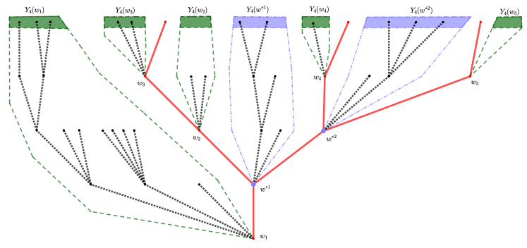
Figure 5. Decomposition of $Z_{4}$ into the total population size of unmarked particles who are descendants of the unmarked offspring of spine particles. The spines are the red lines, the particles $w_{1},w_{2},w_{3},w_{4}$ and $w_{5}$ give birth according to $q_{\cdot}^{(1,\theta)}$ and their unmarked progeny at generation 4 are $(Y_{4}(w_{i}))_{1\leq i\leq 5}$; $w^{*1}$ and $w^{*2}$ give birth according to $q_{\cdot}^{(2,\theta)}$ and their unmarked progeny at generation 4 are $Y_{5}(w^{*1})$ and $Y_{5}(w^{*2})$.

Then Lemma 1 implies

$$\begin{split}\mathbf{Q}^{(e,k,\theta)}_{n}&\left[e^{-(\lambda-\theta)Z_{n}}\Big{|}\psi_{1},\dots,\psi_{k-1},\mathcal{D}_{n},\mathcal{O}=\mathfrak{t}\right]\\ =&\frac{e^{-k\lambda}}{e^{-k\theta}}\prod_{w\in\widetilde{\mathcal{W}}}\frac{f_{|w|+1}^{\prime}(f_{|w|+1,n}(e^{-\lambda}))}{f_{|w|+1}^{\prime}(f_{|w|+1,n}(e^{-\theta}))}\prod_{i=1}^{k-1}\frac{f_{|w^{*i}|+1}^{\prime\prime}(f_{|w^{*i}|+1,n}(e^{-\lambda}))}{f_{|w^{*i}|+1}^{\prime\prime}(f_{|w^{*i}|+1,n}(e^{-\theta}))}\\ =&\frac{e^{-k\lambda}}{e^{-k\theta}}\prod_{w\in\mathcal{W}}\frac{f_{|w|+1}^{\prime}(f_{|w|+1,n}(e^{-\lambda}))}{f_{|w|+1}^{\prime}(f_{|w|+1,n}(e^{-\theta}))}\prod_{i=1}^{k-1}\frac{f_{|w^{*i}|+1}^{\prime\prime}(f_{|w^{*i}|+1,n}(e^{-\lambda}))}{f_{|w^{*i}|+1}^{\prime\prime}(f_{|w^{*i}|+1,n}(e^{-\theta}))}\frac{f_{|w^{*i}|+1}^{\prime}(f_{|w^{*i}|+1,n}(e^{-\theta}))}{f_{|w^{*i}|+1}^{\prime}(f_{|w^{*i}|+1,n}(e^{-\lambda}))}.\end{split}$$

Observe that at every $m\in\{\psi_{i-1}+1,\dots,\psi_{i}\}$, there are $i$ marked particles implying that in the previous decomposition the factor ${f_{m+1}^{\prime}(f_{m+1,n}(e^{-\lambda}))}/{f_{m+1}^{\prime}(f_{m+1,n}(e^{-\theta}))}$ appears $i$ times. Thus by Lemma 1, we obtain

$$\begin{split}\mathbf{Q}^{(e,k,\theta)}_{n}&\left[e^{-(\lambda-\theta)Z_{n}}\Big{|}\psi_{1},\dots,\psi_{k-1},\mathcal{D}_{n},\mathcal{O}=\mathfrak{t}\right]\\ =&\mathbf{Q}^{(e,1,\theta)}_{n}\left[e^{-(\lambda-\theta)Z_{n}}\right]\prod_{i=1}^{k-1}\mathbf{Q}^{(e_{\psi_{i}+1},1,\theta)}_{n-\psi_{i}-1}\left[e^{-(\lambda-\theta)Z_{n-\psi_{i}-1}}\right]\frac{h(n,\psi_{i},\lambda)}{h(n,\psi_{i},\theta)},\end{split}$$

where

$$h(n,m,\lambda):=\frac{f_{m+1}^{\prime\prime}(f_{m+1,n}(e^{-\lambda}))}{f_{m+1}^{\prime}(f_{m+1,n}(e^{-\lambda}))}.$$

We also note that the right-hand side of the previous identity does not depend on the choice $\mathcal{O}=\mathfrak{t}$, in fact we only require to know that the splitting times are different.

Now, if we conditioned on the values of $(\widetilde{\psi}_{1},\dots,\widetilde{\psi}_{k-1})$ instead of $(\psi_{1},\dots,\psi_{k-1})$, we obtain

$$\begin{split}\mathbf{Q}^{(e,k,\theta_{n})}_{n}&\left[e^{-(\lambda-\theta)Z_{n}/a_{n}^{e}}\Big{|}\widetilde{\psi}_{1}=\tau_{n}(t_{1}),\dots,\widetilde{\psi}_{k-1}=\tau_{n}(t_{k-1}),\mathcal{D}_{n},\mathcal{O}=\mathfrak{t}\right]\\ =&\mathbf{Q}^{(e,1,\theta_{n})}_{n}\left[e^{-(\lambda-\theta)Z_{n}/a_{n}^{e}}\right]\prod_{i=1}^{k-1}\mathbf{Q}^{(e_{\tau_{n}(t_{i})+1},1,\theta_{n})}_{n-\tau_{n}(t_{i})-1}\left[e^{-(\lambda-\theta)Z_{n-\tau_{n}(t_{i})-1}/a_{n}^{e}}\right]\frac{h\left(n,\tau_{n}(t_{i}),\lambda/a_{n}^{e}\right)}{h(n,\tau_{n}(t_{i}),\theta/a_{n}^{e})}.\end{split}$$

According to [6, Lemma 3], which also holds under condition ($\filledstar$) (see comments following equation (26)), and the first line of its proof, we deduce

(44) $$\underset{n\rightarrow\infty}{\lim}\ \underset{0\leq m\leq n}{\sup}\left|\frac{h\left(n,\tau_{n}(t_{i}),\lambda/a_{n}^{e}\right)}{h(n,\tau_{n}(t_{i}),\theta/a_{n}^{e})}-1\right|=0.$$

Therefore, by (28) and Lemma 3, we get the result. ∎

With all ingredients in hand, we now proceed with the proof of our main result.

4. Proof of Theorem 1

Proof of Theorem 1.

For a given $\theta\geq 0$, recall that $\mathbf{Q}^{(e,k,\theta_{n})}_{n}$ is the $e^{-\theta_{n}Z_{n}}Z_{n}^{[k]}$-sized biased transform of $\mathbb{P}^{(e)}$ with $\theta_{n}=\theta/a_{n}^{(e)}$. We also recall that $\mathbf{Q}^{(e,k,\theta_{n})}_{n}(Z_{n}\geq k)=1$ and the permuted splitting times are denoted by $(\widetilde{\psi}_{1},\dots,\widetilde{\psi}_{k-1})$. By using conditional probability, we see

(45) $$\begin{split}\mathbb{P}^{(e)}&\left(\widetilde{B}_{1}^{k}(n)\geq\tau_{n}(t_{1}),\dots,\widetilde{B}_{k-1}^{k}(n)\geq\tau_{n}(t_{k-1}),\mathcal{O}=\mathfrak{t}\mid Z_{n}\geq k\right)\\ &=\frac{\mathbb{E}^{(e)}\left[e^{-\theta_{n}Z_{n}}Z_{n}^{[k]}\right]}{(a_{n}^{(e)})^{k}\mathbb{P}^{(e)}\left(Z_{n}\geq k\right)}\mathbf{Q}^{(e,k,\theta_{n})}_{n}\left[\frac{e^{\theta_{n}Z_{n}}}{(a_{n}^{(e)})^{-k}Z_{n}^{[k]}}\mathbf{1}_{\{\widetilde{\psi}_{1}\geq\tau_{n}(t_{1}),\dots,\widetilde{\psi}_{k-1}\geq\tau_{n}(t_{k-1})\},}\mathcal{O}=\mathfrak{t}\right].\end{split}$$

Now, similarly as before we complete the factors with $F_{k,n,0}$ defined in (33) and use conditional probability, to obtain

$$\begin{split}\frac{\mathbb{E}^{(e)}\left[e^{-\theta_{n}Z_{n}}Z_{n}^{[k]}\right]}{(a_{n}^{(e)})^{k}\mathbb{P}^{(e)}\left(Z_{n}\geq k\right)}=\left(\frac{k!\ F_{k,n,0}}{(1+\theta)^{k+1}}\right)\left(\frac{\mu_{n}^{(e)}}{a_{n}^{(e)}\mathbb{P}^{(e)}\left(Z_{n}>0\right)}\right)\left(\frac{1}{\mathbb{P}^{(e)}\left(Z_{n}\geq k\mid Z_{n}>0\right)}\right).\end{split}$$

According to equation (3), the second fraction in the right hand side of the above identity goes to $1$, as $n\rightarrow\infty$. Moreover, Proposition 7 implies that $Z_{n}$ conditioned on $\{Z_{n}>0\}$ goes to $\infty$, as $n\rightarrow\infty$, which implies $\mathbb{P}^{(e)}\left(Z_{n}\geq k\mid Z_{n}>0\right)\rightarrow 1.$ Then, by Lemma 2, we have

(46) $$\underset{n\rightarrow\infty}{\lim}\frac{\mathbb{E}^{(e)}\left[e^{-\theta_{n}Z_{n}}Z_{n}^{[k]}\right]}{(a_{n}^{(e)})^{k}\mathbb{P}^{(e)}\left(Z_{n}\geq k\right)}=\frac{k!}{(1+\theta)^{k+1}}.$$

Therefore, the result holds as soon as we compute the asymptotic behaviour of the second term in the right-hand side of (45). First, we observe that $(Z_{n}-k)^{-k}\leq(Z_{n}^{[k]})^{-1}\leq(Z_{n})^{-k}$ and $a_{n}^{(e)}\rightarrow\infty$, as $n\rightarrow\infty$. This implies that the aforementioned limit is the same as

$$\underset{n\rightarrow\infty}{\lim}\mathbf{Q}^{(e,k,\theta_{n})}_{n}\left[\frac{e^{\theta_{n}Z_{n}}}{\left((a_{n}^{(e)})^{-1}Z_{n}\right)^{k}}\mathbf{1}_{\{\widetilde{\psi}_{1}\geq\tau_{n}(t_{1}),\dots,\widetilde{\psi}_{k-1}\geq\tau_{n}(t_{k-1})\}},\mathcal{O}=\mathfrak{t}\right].$$

Now, if we use the following identity

(47) $$\frac{e^{\theta x}}{x^{k}}=\int_{0}^{\infty}\frac{\lambda^{k-1}}{(k-1)!}e^{-(\lambda-\theta)x}\,\mathrm{d}\lambda,$$

we obtain

$$\begin{split}&\mathbf{Q}^{(e,k,\theta_{n})}_{n}\left[\frac{e^{\theta_{n}Z_{n}}}{\left((a_{n}^{(e)})^{-1}Z_{n}\right)^{k}}\mathbf{1}_{\{\widetilde{\psi}_{1}\geq\tau_{n}(t_{1}),\dots,\widetilde{\psi}_{k-1}\geq\tau_{n}(t_{k-1})\}},\mathcal{O}=\mathfrak{t}\right]=\int_{0}^{\infty}\frac{\lambda^{k-1}}{(k-1)!}f_{n}(\lambda)\,\mathrm{d}\lambda,\end{split}$$

where the function $f_{n}$ is defined by

$$\begin{split}f_{n}(\lambda):&=\mathbf{Q}^{(e,k,\theta_{n})}_{n}\left[e^{-(\lambda-\theta)Z_{n}/a_{n}^{e}}\mathbf{1}_{\{\widetilde{\psi}_{1}\geq\tau_{n}(t_{1}),\dots,\widetilde{\psi}_{k-1}\geq\tau_{n}(t_{k-1})\}},\mathcal{O}=\mathfrak{t}\right].\end{split}$$

Next, recall that $\mathcal{D}_{n}$ denotes the event that all spines splitting times are different. By conditioning on the values of $(\widetilde{\psi}_{1},\dots,\widetilde{\psi}_{k-1})$ and $\mathcal{O}=\mathfrak{t}$, we have that

$$\begin{split}&f_{n}(\lambda)=\mathbf{Q}^{(e,k,\theta_{n})}_{n}\left[e^{-(\lambda-\theta)Z_{n}/a_{n}^{e}}\mathbf{1}_{\{\widetilde{\psi}_{1}\geq\tau_{n}(t_{1}),\dots,\widetilde{\psi}_{k-1}\geq\tau_{n}(t_{k-1})\}},\mathcal{O}=\mathfrak{t},\mathcal{D}_{n}^{c}\right]+\\ &\mathbf{Q}^{(e,k,\theta_{n})}_{n}\left[\mathbf{Q}^{(e,k,\theta_{n})}_{n}\left[e^{-(\lambda-\theta)Z_{n}/a_{n}^{e}}\mid\widetilde{\psi}_{1},\dots,\widetilde{\psi}_{k-1},\mathcal{O},\mathcal{D}_{n}\right]\mathbf{1}_{\{\widetilde{\psi}_{1}\geq\tau_{n}(t_{1}),\dots,\widetilde{\psi}_{k-1}\geq\tau_{n}(t_{k-1})\}},\mathcal{O}=\mathfrak{t},\mathcal{D}_{n}\right]\end{split}$$

Since $\underset{n\rightarrow\infty}{\lim}\mathbf{Q}^{(e,k,\theta_{n})}_{n}\left(\mathcal{D}_{n}\right)=1$, we may use Corollary 1 and Lemma 4, to see

$$\begin{split}f_{n}(\lambda)\underset{n\rightarrow\infty}{\longrightarrow}&\mathbb{P}_{\mathcal{B}^{k}}(\mathfrak{t})\frac{(1+\theta)^{k+1}}{(1+\lambda)^{2}}\prod_{i=1}^{k-1}\int_{t_{i}}^{1}\frac{1}{(1+\lambda(1-r_{i}))^{2}}\,\mathrm{d}r_{i}\\ &=\mathbb{P}_{\mathcal{B}^{k}}(\mathfrak{t})\frac{(1+\theta)^{k+1}}{(1+\lambda)^{2}\lambda^{k-1}}\prod_{i=1}^{k-1}\left(1-\frac{1}{1+\lambda(1-t_{i})}\right).\end{split}$$

Now, we define the function $g_{n}(\lambda):=\mathbf{Q}^{(e,k,\theta_{n})}_{n}\left[e^{-(\lambda-\theta)Z_{n}/a_{n}^{e}}\right]$. Then, by the definition of $f_{n}$ and Lemma 3, we deduce

$$f_{n}(\lambda)\leq g_{n}(\lambda)\underset{n\rightarrow\infty}{\longrightarrow}\frac{(1+\theta)^{k+1}}{(1+\lambda)^{k+1}}.$$

Additionally, if we use again equation (47), we get

$$\int_{0}^{\infty}\frac{\lambda^{k-1}}{(k-1)!}g_{n}(\lambda)\,\mathrm{d}\lambda=\mathbf{Q}^{(e,k)}_{n}\left[\frac{e^{\theta_{n}Z_{n}}}{\left((a_{n}^{(e)})^{-1}Z_{n}\right)^{k}}\right]\sim\mathbf{Q}^{(e,k,\theta_{n})}_{n}\left[\frac{e^{\theta_{n}Z_{n}}}{(a_{n}^{(e)})^{-k}Z_{n}^{[k]}}\right],\quad\textrm{as }n\rightarrow\infty.$$

Therefore, by using (45) with $0=t_{1}=\cdots=t_{k-1}$ and (46), we get

$$\int_{0}^{\infty}\frac{\lambda^{k-1}}{(k-1)!}g_{n}(\lambda)\,\mathrm{d}\lambda\longrightarrow\frac{(1+\theta)^{k+1}}{k!}=\int_{0}^{\infty}\frac{\lambda^{k-1}}{(k-1)!}\frac{(1+\theta)^{k+1}}{(1+\lambda)^{k+1}}\,\mathrm{d}\lambda.$$

Then, we apply the extended Dominated Convergence Theorem (see for instance [13, Theorem 1.23],) with the sequence of functions $\{\lambda^{k-1}f_{n}(\lambda):n\geq 1\}$ and $\{\lambda^{k-1}g_{n}(\lambda):n\geq 1\}$ in order to obtain

$$\begin{split}&\underset{n\rightarrow\infty}{\lim}\mathbf{Q}^{(e,k,\theta_{n})}_{n}\left[\frac{e^{\theta_{n}Z_{n}}}{\left((a_{n}^{(e)})^{-1}Z_{n}\right)^{k}}\mathbf{1}_{\{\widetilde{\psi}_{1}\geq\tau_{n}(t_{1}),\dots,\widetilde{\psi}_{k-1}\geq\tau_{n}(t_{k-1})\}},\mathcal{O}=\mathfrak{t}\right]\\ &\hskip 56.9055pt=\mathbb{P}_{\mathcal{B}^{k}}(\mathfrak{t})\frac{(1+\theta)^{k+1}}{(k-1)!}\int_{0}^{\infty}\frac{1}{(1+\lambda)^{2}}\prod_{i=1}^{k-1}\left(1-\frac{1}{1+\lambda(1-t_{i})}\right)\,\mathrm{d}\lambda.\end{split}$$

Thus, combining with equations (45) and (46), we have

(48) $$\begin{split}\underset{n\rightarrow\infty}{\lim}\mathbb{P}^{(e)}&\left(\widetilde{B}_{1}^{k}(n)\geq\tau_{n}(t_{1}),\dots,\widetilde{B}_{k-1}^{k}(n)\geq\tau_{n}(t_{k-1}),\mathcal{O}=\mathfrak{t}\mid Z_{n}\geq k\right)\\ &=\mathbb{P}_{\mathcal{B}^{k}}(\mathfrak{t})\int_{0}^{\infty}\frac{k}{(1+\lambda)^{2}}\prod_{i=1}^{k-1}\left(1-\frac{1}{1+\lambda(1-t_{i})}\right)\,\mathrm{d}\lambda.\\ &=\mathbb{P}_{\mathcal{B}^{k}}(\mathfrak{t})\int_{0}^{\infty}\frac{k\lambda^{k-1}}{(1+\lambda)^{k+1}}.\left(\prod_{i=1}^{k-1}\int_{t_{i}}^{1}\frac{(1+\lambda)}{\left(1+\lambda(1-s_{i})\right)^{2}}\,\mathrm{d}s_{i}\right)\,\mathrm{d}\lambda.\\ \end{split}$$

Observe that the previous integral is the corresponding joint distribution of the density found in [11, proof of Theorem 4]. Note, we can construct the coalescent times by renormalising by the maximum of $k$ independent random variable with density $(1+x)^{2}$ for $x\in(0,1)$. Alternatively, we can view the coalescent times as a mixture of independent random variables. Finally, by computing this integral explicitly, equivalently taking $e_{0}=1$ and $e_{i}=1-t_{i}$ for $i=1,\dots,k-1$ in [12, Lemma 34], we deduce the result. This completes the proof. ∎

References

- [1] R. Abraham and P. Debs. Penalization of Galton–Watson processes Stochastic Processes and their Applications, 130(5), 2020.
- [2] V. Bansaye and F. Simatos. On the scaling limits of Galton-Watson processes in varying environments. Electronic Journal of Probability, 20, 2015.
- [3] N. Bhattacharya and M. Perlman. Time-inhomogeneous branching processes conditioned on non-extinction. arXiv preprint arXiv:1703.00337, 2017.
- [4] P. Billingsley. Convergence of probability measures. Wiley Series in Probability and Statistics: Probability and Statistics, 1999. Second edition.
- [5] F. Boenkost, F. Foutel–Rodier, E. Schertzer. The genealogy of a nearly critical branching processes in varying environment. Preprint, 2022.
- [6] N. Cardona-Tobón and S. Palau. Yaglom’s limit for critical Galton-Watson processes in varying environment: a probabilistic approach. Bernoulli, 27(3):1643–1665, 2021.
- [7] R. Fang, Z. Li, and J. Liu. A scaling limit theorem for galton–watson processes in varying environments. Proceedings of the Steklov Institute of Mathematics, 316(1):137–159, 2022.
- [8] M. González, G. Kersting, C. Minuesa, and I. del Puerto. Branching processes in varying environment with generation-dependent immigration. Stochastic Models, 35(2):148–166, 2019.
- [9] S. C. Harris, S. G. Johnston, and J. C. Pardo. Universality classes for the coalescent structure of heavy-tailed Galton-Watson trees. Work in progress, 2022.
- [10] S. C. Harris, S. Palau, and J. C. Pardo. The coalescent structure of GW trees in linear fractional environments with applications. Work in progress, 2022.
- [11] S. C. Harris, S. G. Johnston, and M. I. Roberts. The coalescent structure of continuous-time Galton–Watson trees. The Annals of Applied Probability, 30(3):1368–1414, 2020.
- [12] S. C. Harris, S. G. G. Johnston, and M. I. Roberts. The coalescent structure of continuous-time Galton-Watson trees. arXiv:1703.00299 (v4), 2017.
- [13] O. Kallenberg. Foundations of modern probability, volume 99 of Probability Theory and Stochastic Modelling. Springer, Cham, 2021. Third edition.
- [14] G. Kersting. A unifying approach to branching processes in varying environments. Journal of Applied Probability, 57(1):196–220, 2020.
- [15] G. Kersting. On the genealogical structure of critical branching processes in a varying environment. Proceedings of the Steklov Institute of Mathematics, 316(1):209–219, 2022.
- [16] G. Kersting and V. A. Vatutin. Discrete time branching processes in random environment. Wiley Online Library, 2017.
- [17] I. MacPhee and H. Schuh. A Galton-Watson branching process in varying environments with essentially constant offspring means and two rates of growth. Australian Journal of Statistics, 25(2):329–338, 1983.