Small Schwarzschild de Sitter black holes,
quantum extremal surfaces and islands

Kaberi Goswami,  K. Narayan

Chennai Mathematical Institute,
SIPCOT IT Park, Siruseri 603103, India.

We study 4-dimensional Schwarzschild de Sitter black holes in the regime where the black hole mass is small compared with the de Sitter scale. Then the de Sitter temperature is very low compared with that of the black hole and we study the black hole, approximating the ambient de Sitter space as a frozen classical background. We consider distant observers in the static diamond, far from the black hole but within the cosmological horizon. Using 2-dimensional tools, we find that the entanglement entropy of radiation exhibits linear growth in time, indicative of the information paradox for the black hole. Self-consistently including an appropriate island emerging at late times near the black hole horizon leads to a reasonable Page curve. There are close parallels with flat space Schwarzschild black holes in the regime we consider.

1 Introduction

The black hole information paradox [2] can be regarded as the tension between the apparent unbounded growth of entanglement entropy of thermal Hawking radiation [3] outside the black hole and the expectation from quantum mechanics that entanglement entropy must become small at late times if purity of the original matter state is to be recovered, i.e. it must follow the Page curve [4, 5]. See e.g. [6, 7] for discussions of various aspects of the information paradox. Recent exciting discoveries unravelled via the study of entanglement and quantum extremal surfaces [8, 9, 10, 11, 12] have found that including nontrivial “island” contributions does in fact do this job. Quantum extremal surfaces are extrema of the generalized gravitational entropy [13, 14] obtained from the classical area of the entangling RT/HRT surface [15]-[18] after incorporating the bulk entanglement entropy of matter, with explicit calculation possible in effective 2-dimensional models where 2-dim CFT techniques enable detailed analysis of the bulk entanglement entropy. The island, arising as a nontrivial solution to extremization (near the black hole horizon, and only at late times), reflects new replica wormhole saddles [11, 12] and serves to purify the early Hawking radiation thereby leading to the entanglement entropy decreasing. There is a large body of literature on various aspects of these issues, reviewed in e.g. [19, 20, 21]: see e.g. [22]-[61] for a partial list of investigations on black holes in this regard. Scrutinies of the island formulation and alternative perspectives appear in e.g. [62, 63, 64].

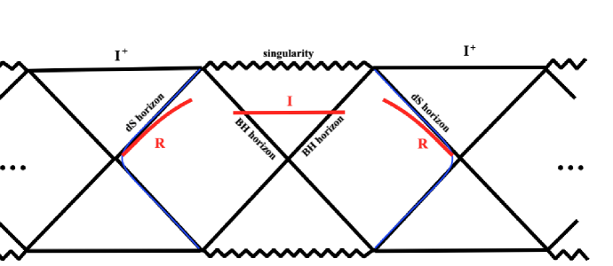
In this paper, we study “small” Schwarzschild de Sitter black holes, i.e. the regime where the black hole mass $m$ is small compared with the de Sitter scale $l$, but large enough that a quasi-static approximation to the geometry is valid. This translates to saying that the de Sitter temperature is very low compared with that of the black hole. In this regime, we approximate the ambient de Sitter space as a frozen classical background and study the two-sided (eternal) black hole. We can imagine that the black hole has formed from initial matter in a pure state: strictly speaking this can only be an approximation to the bulk CFT at the thermal state at the de Sitter temperature, but it is a reasonable approximation if the de Sitter temperature is very low. We focus on one black hole coordinate patch in the Penrose diagram, Figure 1 (which roughly comprises a line of alternating Schwarzschild and de Sitter patches), and consider observers in the static diamond patches far outside the black hole but within the cosmological horizons which bound the black hole patch, Figure 2. Then the entanglement entropy of the radiation exhibits an unbounded linear growth in time, which is inconsistent at late times with the entropy of the black hole, and indicative of the information paradox for the black hole. Using the island rule in the extremization of the generalized entropy shows an island emerging at late times a little outside the black hole horizon semiclassically: this then shows finiteness of the entanglement entropy of radiation recovering the expectations on the Page curve. In some essential sense, our analysis (which is purely bulk, with no holography per se) closely mirrors island studies of flat space Schwarzschild black holes in the literature, with the ambient de Sitter space entering only through more complicated coordinates.

In sec. 2, we review 4-dim Schwarzschild de Sitter black holes as required for our purposes, and in sec. 3, we describe our setup for the generalized entropy via 2-dim techniques. Sec. 3.1 discusses the entanglement entropy in the absence of the island (with details in App. A), while sec. 4 discusses the island calculation (details in App. B; see also App. C for early times). Finally sec. 5 contains a Discussion of our approximations and open questions.

2 Small Schwarzschild de Sitter black holes $\rightarrow$ 2-dim

The Schwarzschild de Sitter black hole spacetime in $3+1$-dimensions has the metric

$$ds^{2}=-f(r)dt^{2}+\frac{dr^{2}}{f(r)}+r^{2}d\Omega_{2}^{2}\ ,\qquad f(r)=1-\frac{2m}{r}-\frac{r^{2}}{l^{2}}\ .$$ (1)

This is a Schwarzschild black hole in de Sitter space [65] with an “outer” cosmological (de Sitter) horizon and an “inner” Schwarzschild horizon. The surface gravity at both horizons is generically distinct: Euclidean continuations removing a conical singularity can be defined at each horizon separately but not simultaneously at both [66] (see also [67, 68]). The only (degenerate) exception is in an extremal, or Nariai, limit [69] where both periodicities of Euclidean time match: the spacetime develops a nearly $dS_{2}$ throat in this extremal limit [66]. More on the nearly $dS_{2}$ limit and the wavefunction of the universe appears in [70] (see also [71]). Related discussions with some relevance to this paper also appear in [72].

The general $d+1$-dimensional SdS spacetime is of similar form as (1) but with $f(r)=1-\frac{2m}{l}(\frac{l}{r})^{d-2}-\frac{r^{2}}{l^{2}}$, and will have qualitative parallels. We will focus on the 4-dim Schwarzschild de Sitter case in what follows. For $SdS_{4}$, the function $f(r)$ is a cubic and the zeroes of $f(r)$, i.e. solutions to $f(r)=0$, give the locations of the horizons. We can parametrize this as

$$f(r)=1-\frac{2m}{r}-\frac{r^{2}}{l^{2}}=\frac{1}{l^{2}\,r}\,(r_{D}-r)(r-r_{S})(r+r_{S}+r_{D})\,,\qquad\qquad\qquad$$

$$r_{D}r_{S}(r_{D}+r_{S})=2ml^{2}\,,\qquad r_{D}^{2}+r_{D}r_{S}+r_{S}^{2}=l^{2}\ ;\qquad 0\leq r_{S}\leq r_{D}\leq l\ ;\qquad{m\over l}\leq{1\over 3\sqrt{3}}\ .$$ (2)

We will take the roots $r_{S}$ and $r_{D}$ to label the Schwarzschild black hole and de Sitter (cosmological) horizons respectively. (The third zero $-(r_{D}+r_{S})$ does not correspond to a physical horizon.) The roots $r_{S},r_{D}$ are constrained as above.

Figure 1: The Schwarzschild de Sitter black hole Penrose diagram, with focus on one black hole “patch”.

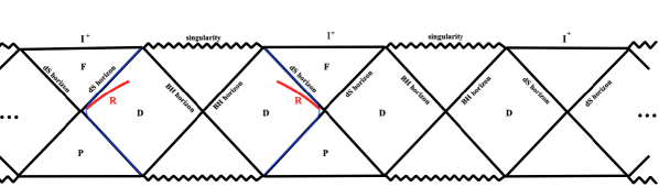
The case with $m=0$, or $r_{S}=0,\ r_{D}=l$, is pure de Sitter space, while the flat space Schwarzschild black hole has $l=0$, or $r_{S}=m,\ r_{D}=0$. The above structure of horizons is valid for ${m\over l}<{1\over 3\sqrt{3}}$ , beyond which there are no horizons [65]. The limit ${m\over l}={1\over 3\sqrt{3}}$ corresponds to the cosmological and Schwarzschild horizon values coinciding: here we have $r_{S}=r_{D}=r_{0}={l\over\sqrt{3}}$ from (2). This special value leads to the extremal, or Nariai, limit where the near horizon region (between the horizons) becomes $dS_{2}\times S^{2}$. Overall the range of physically interesting $r_{S},r_{D}$ satisfies $0<r_{S}<r_{0}<r_{D}$ for generic values. The fact that $r_{S}<r_{D}$ implies that the cosmological horizon is “outside” the Schwarzschild one. The black hole interior has $r<r_{S}$ with $r\rightarrow 0$ the singularity. The region $r_{D}<r\leq\infty$ describes the future and past de Sitter universes, with $r\rightarrow\infty$ the future boundary $I^{+}$ (or past, $I^{-}$). The maximally extended Penrose diagram Figure 1 shows an infinitely repeating pattern of Schwarzschild coordinate patches or “unit-cells” containing Schwarzschild black hole horizons cloaking interior regions: these patches are bounded by cosmological horizons on the left and right, with future/past universes beyond the cosmological horizons.

The intermediate static diamond region $D$ is the exterior of the black hole, i.e. the static patch with a timelike Killing vector where physical timelike observers can be stationary:

$$D:\qquad r_{S}<r<r_{D}\ ;\qquad 0<f(r)<1\ .$$ (3)

We want to consider the limit of a “small” black hole in de Sitter, i.e.

$$m\ll l\,,\qquad\quad l\rightarrow{\rm large}\qquad\Rightarrow\qquad r_{D}\gg r_{S}\ .$$ (4)

The horizon locations can then be found perturbatively to be $r_{S}\simeq 2m\,,\ r_{D}\simeq l-m\gg r_{S}$ , from (2). In this limit (in a sense opposite to the Nariai limit where $r_{S}\sim r_{D}$), the black hole is much smaller than the ambient de Sitter scale, i.e. we have a small black hole in a large accelerating universe. So we expect that the ambient cosmology can be taken as a frozen classical background while the black hole undergoes Hawking evaporation. This is corroborated by the fact that the black hole Hawking temperature is much larger than the Gibbons-Hawking temperature of the ambient de Sitter horizon: i.e. using the surface gravities $\kappa$ [67, 68] (see also [73]) and $T={\kappa\over 2\pi}$ we obtain in the limit (4),

$$T_{BH}\sim{1\over 8\pi m}\ ,\qquad T_{dS}\sim{1\over 2\pi l}\ ;\qquad\qquad T_{dS}\ll T_{BH}\ .$$ (5)

Pushing this to the extreme leads to the flat space limit

$$r_{D}\sim l\rightarrow\infty\,:\qquad{r_{D}\over l}\rightarrow 1\ ,\qquad r_{S}\rightarrow 2m\ ;\qquad\quad T_{dS}\rightarrow 0\ ,$$ (6)

where the ambient de Sitter background acquires a vanishingly small temperature, approaching asymptotically flat space. Our entire analysis will in fact focus on these limits (4), (5), with the flat limit (6) as a special case to corroborate with.

Towards analysing the generalized entropy, we will require recasting the Schwarzschild de Sitter metric (1) in Kruskal coordinates which are regular at the black hole horizon. These are not regular in the vicinity of the de Sitter horizon (where a distinct set of Kruskal variables is more appropriate), but we will find that the black hole Kruskal variables suffices for our considerations. This is consistent with the fact the ambient de Sitter space simply serves as a frozen classical background in our regimes of interest. With this in mind, we define the black hole tortoise coordinate following the discussion in [74] :

$$r^{\ast}=\int\frac{1}{f(r)}\,dr=\int\frac{1}{1-\frac{2m}{r}-\frac{r^{2}}{l^{2}}}\ dr=\int\frac{l^{2}r}{(r_{D}-r)(r-r_{S})(r+r_{S}+r_{D})}\ dr\ .$$ (7)

Taking $f(r)>0$ as pertains to the region $D$ in (3), this gives

$$e^{r^{\ast}}=(r_{D}-r)^{-\beta_{D}}(r-r_{S})^{\beta_{s}}(r+r_{D}+r_{S})^{\beta_{M}}\ ,$$ (8)

with the parameters (which simplify $dr^{\ast}/dr$ to $1/f(r)$)

$$\beta_{D}=\frac{l^{2}r_{D}}{(r_{D}-r_{S})(2r_{D}+r_{S})}\,,\quad\beta_{S}=\frac{l^{2}r_{S}}{(r_{D}-r_{S})(2r_{S}+r_{D})}\,,\quad\beta_{M}=\frac{l^{2}(r_{D}+r_{S})}{(2r_{D}+r_{S})(2r_{S}+r_{D})}\,.$$ (9)

In the flat limit (6), $\beta_{S}\rightarrow r_{S}$ and $\beta_{D}\rightarrow l$.

The $SdS_{4}$ metric (1) is recast as $ds^{2}=f(r)(-dt^{2}+{dr^{\ast}}^{2})+r^{2}d\Omega_{2}^{2}$ . In the neighborhood of the black hole horizon, the Kruskal coordinates are then defined as $U_{S},\,V_{S}$ , and the Schwarzschild de Sitter metric becomes [74]

$$\alpha_{S}=\frac{1}{2\beta_{S}}\,;\qquad U_{S}V_{S}=-e^{2\alpha_{S}r^{\ast}}\ ,\qquad{U_{S}\over V_{S}}=-e^{-2\alpha_{S}t}\ ;\qquad ds^{2}=-\frac{dU_{S}dV_{S}}{W^{2}}+r^{2}d\Omega^{2}\ ,$$

$$W=\sqrt{r}\,l\,\alpha_{S}(r_{D}-r)^{\frac{-(1+2\alpha_{S}\beta_{D})}{2}}(r-r_{S})^{\frac{2\alpha_{S}\beta_{S}-1}{2}}(r+r_{S}+r_{D})^{\frac{2\alpha_{S}\beta_{M}-1}{2}}\ .\qquad$$ (10)

The value of $\alpha_{S}$ here ensures regularity at the black hole horizon. (noting $\beta_{M}+\beta_{S}=\beta_{D}$ we see that $W$ has dimensions of inverse length.) The Kruskal coordinates cover both the left and right static diamonds $D$ of the black hole patch: in the right side (containing $R_{+}$ in Figure 1) we define

$$U_{S}=-e^{-\alpha_{S}(t-r^{\ast})}\,,\qquad V_{S}=e^{\alpha_{S}(t+r^{\ast})}\ ,$$ (11)

while on the left side (with $R_{-}$) there is a relative minus sign, i.e. $U_{S}\rightarrow-U_{S},\ V_{S}\rightarrow-V_{S}$.

For our purposes, it is a reasonable approximation to look at the s-wave sector of the black hole and consider the bulk matter as a 2-dim CFT: this enables the use of 2-dim CFT tools to study the entanglement entropy of bulk matter. With this in mind, we consider a reduction ansatz of the form

$$ds^{2}_{(4)}=g^{(2)}_{\mu\nu}dx^{\mu}dx^{\nu}+\lambda^{-2}\phi\,d\Omega_{2}^{2}\ ;\qquad\quad g_{\mu\nu}=\phi^{1/2}\,g^{(2)}_{\mu\nu}\ ,$$ (12)

to obtain 2-dimensional dilaton gravity [75, 76] (see also [77]; applications to certain families of cosmologies appears in [78]). The lengthscale $\lambda^{-1}$ has been introduced to make the dilaton dimensionless. The dilaton $\phi$ translates to the 4-dim transverse area of 2-spheres $4\pi\phi\over\lambda^{2}$ . The final term represents a Weyl transformation to absorb the dilaton kinetic term giving ${1\over 16\pi G_{2}}\int d^{2}x\sqrt{-g}\ (\phi{\cal R}-{6\over l^{2}}\phi^{1/2}+2\lambda^{2}\phi^{-1/2})$ as the 2-dim action. The 2-dim metric and dilaton are

$$ds^{2}=-\lambda\,r\frac{dU_{S}dV_{S}}{W^{2}}\,\equiv\,-\frac{dU_{S}dV_{S}}{(W^{\prime})^{2}}\ ,\qquad\qquad\phi=r^{2}\lambda^{2}\ ,$$ (13)

where $W^{\prime}={W\over\sqrt{\lambda\,r}}$ and $W$ is the conformal factor given in (2). For our discussions of entanglement entropy in these 2-dim theories, $\lambda$ will be regarded as some fixed length scale independent of the de Sitter scale $l$ so as to not interfere with the flat limit. With $G_{{}_{N}}$ the 4-dim Newton constant, $G_{2}={G_{{}_{N}}\over V_{2}}$ and $V_{2}={4\pi\over\lambda^{2}}$ , the area term in the 2-dim theory is ${\phi\over 4G_{2}}={4\pi\,r^{2}\over 4G_{{}_{N}}}$ equivalent to the 4-dim one.

Figure 2: The Penrose diagram of a Schwarzschild de Sitter black hole, with focus on one black hole “patch” bounded by cosmological horizons on both sides. Depicted are the radiation regions $R_{-}\equiv[r_{D-},b_{-}]$ and $R_{+}\equiv[b_{+},r_{D+}]$ and the late time island $I\equiv[a_{-},a_{+}]$.

3 Black holes in de Sitter and entanglement entropy

In the regimes (4), (5), that we are considering, we see that there is a version of the information paradox for the black hole that is at play, with some parallels with that for the eternal $AdS$ black hole in [22]. If the black hole forms from initial collapsing matter in a pure state, then information recovery at late times compared with the black hole timescale requires that the generalized gravitational entropy of the radiation obeys the Page curve. Note that in the current situation, this is only approximate since the ambient de Sitter space is only consistent with bulk CFT matter in a thermal state at the de Sitter temperature. However if the ambient de Sitter temperature is very low, then one might imagine that a pure state approximation is reasonable. This is the limit (5) we study to understand the black hole evaporation process here, which we find to be consistent. We will find, as in various previous investigations, that a nontrivial island emerges at late times a little outside the horizon as a nontrivial quantum extremal surface solution to the extremization of the generalized gravitational entropy. Including this and using the island rule shows the late time entropy to be bounded. Our analysis has close parallels with that of flat space Schwarzschild black holes e.g. [26, 27], our expressions showing essential agreement in the flat space limit (6).

In our case, we consider distant observers that are stationary, represented by timelike worldlines in the static patch $D$ region (3), between the Schwarzschild and de Sitter (cosmological) horizons. Towards simulating the flat space limit, we will consider the far end of the radiation region as asymptoting to the cosmological horizon. The outgoing radiation hits the cosmological horizon and as such is expected to go beyond and eventually hit the future boundary $I^{+}$ (future timelike infinity). However we assume that the observers propagating in the static patch $D$ collect this outgoing radiation. So we will focus on the Schwarzschild patch bounded by the cosmological horizons on both sides and ignore the regions beyond: see Figure 2.

The island proposal [10] for the fine-grained entropy of the Hawking radiation is

$$S(R)=min\left\{{ext\Big{[}\frac{Area(\partial I)}{4G_{{}_{N}}}+S_{matter}(R\cup I)\Big{]}}\right\}$$ (14)

where $R$ is a region far from the black hole where the radiation is collected by distant observers and $I$ is a spatially disconnected island around the horizon that is entangled with $R$. The intuition behind this expression is that after about half the black hole has evaporated, the Hawking radiation going out (roughly $I$) begins to purify the radiation that was emitted early on (roughly $R$). This purification of the early radiation by the late Hawking radiation is a reflection of the entanglement between the two parts, and stems from the picture of Hawking radiation as due to production of entangled particle pairs near the horizon (which is taken as vacuum). Thus $R\cup I$ purifies over time and its entanglement thus does not grow: the slowly evaporating black hole has decreasing area, so $S(R)$ decreases in time.

The Hawking process is dominated by s-wave modes. So we calculate the bulk entropy technically using 2-dimensional techniques where we approximate the bulk matter by a 2-dim CFT propagating in the 2-dim background obtained by dimensional reduction. In what follows, we will employ these techniques to calculate the entanglement entropy in the Schwarzschild de Sitter geometry by considering the 2-dim background (13) obtained from the reduction of (2). There is no holography in our entire discussion here: we are simply calculating the entropy of radiation in the bulk spacetime using the island rule (14).

In the absence of the island, the radiation regions are given by the intervals $R_{\pm}\in D$,

$$R=R_{-}\cup R_{+}\ ;\qquad R_{-}\equiv[r_{D-},b_{-}]\,,\quad R_{+}\equiv[b_{+},r_{D+}]\ ,$$ (15)

which are the two regions marked in the Figure, one in either asymptotic region of the black hole patch. Since the radiation region is far from the black hole horizon, we have $b_{\pm}-r_{S}\gg r_{S}$. The entropy of the Hawking radiation is

$$S_{matter}=S(R)\ .$$ (16)

In the 2-dim CFT, the matter entanglement entropy for a single interval $A=[x,y]$ is obtained from the replica formulation [79, 80] after also incorporating in $d[x,y]$ the conformal transformation to a curved space [9], stemming from the $W^{\prime}$-factor in the 2-dim metric (13),

$$S_{A}=\frac{c}{3}\log{d[x,y]}\,=\,{c\over 6}\log\left({-\Delta U_{S}\Delta V_{S}\over W^{\prime}|_{x}\,W^{\prime}|_{y}}\right)\ .$$ (17)

From (13), we see that there is one factor of $\lambda$ that arises inside the logarithm in each expression of the last form: in addition there is the ultraviolet cutoff $\epsilon_{UV}$ as in footnote 2. This factor ${\lambda\over\epsilon_{UV}^{2}}$ in each such term will not play much role and we will ignore this except where necessary.

The entanglement entropy for multiple disjoint intervals

$$A=[x_{1},y_{1}]\ \cup\ [x_{2},y_{2}]\ \cup\ \ ....\ \ \cup\ [x_{N},y_{N}]$$ (18)

is more complicated: this arises from the multi-point correlation functions of twist operators and so it depends on not just the central charge but detailed CFT information. In the limit where the intervals are well-separated, one can expand the twist operator products and obtain [79, 80, 81, 82]

$$S_{A}=\frac{c}{3}\,\log\,{\prod_{i,j}d[x_{j},y_{i}]\over\,\prod_{i<j}d[x_{j},x_{i}]\ \ \prod_{i<j}d[y_{j},y_{i}]\,}$$ (19)

For two intervals $[x_{1},y_{1}]\cup[x_{2},y_{2}]$, this is a limit where the cross ratio $x$ is small, i.e.

$$x={\,d[x_{1},y_{1}]\,d[x_{2},y_{2}]\,\over\,d[x_{1},x_{2}]\,d[y_{1},y_{2}]\,}\ ;\qquad x\ll 1\ ,$$ (20)

where we use the Kruskal distances in (17) in constructing the cross-ratio. In 2-dim CFTs with a holographic dual, this is the situation where the two intervals $A,B$ are well-separated and their mutual information exhibits a disentangling transition [83] with $I[A,B]=S[A]+S[B]-S[A\cup B]\rightarrow 0$, i.e. the disconnected surface $S_{dis}=S[A]+S[B]$ has lower area than the connected surface $S_{conn}=S[A\cup B]$. It turns out that the cross-ratio for the points in question becomes small at late times, as we will see later, justifying the use of (19) for our purposes.

In what follows, we first calculate the entanglement entropy for the configuration without any island, using 16: this shows the entropy of radiation as increasing linearly in time at late times, indicative of the information paradox. Towards resolving this we will include a possible island and calculate the entanglement entropy using the island rule 14: this results in a late time entropy that is time-independent.

3.1 Entanglement entropy: no island

In this section, we will evaluate the entanglement entropy of the radiation at late times in the absence of any island. Then we have only the radiation regions $R_{-}\cup R_{+}$ in Figure 2, given by the intervals (15), i.e. $R_{-}\equiv[r_{D-},b_{-}]$ and $R_{+}\equiv[b_{+},r_{D+}]$. In the limit (4), (5), with the de Sitter temperature very low, we can approximate the entire system as a pure state on any slice. Then the bulk matter CFT entropy of $R$ is the same as that of the complementary region $R_{c}=[b_{-},b_{+}]$, so we obtain

$$S_{matter}=\frac{c}{3}\,\log\,[d(b_{+},b_{-})]\ .$$ (21)

We label the spacetime coordinates in the left and right asymptotic regions in the Schwarzschild patch as

$$b_{+}:\ \ \ (t,r)=(t_{b},b)\ ,\qquad b_{-}:\ \ \ (t,r)=(-t_{b}+\frac{i\beta}{2},b)\ ;\qquad\quad\beta=\frac{2\pi}{\alpha_{S}}\ .$$ (22)

This choice of $\beta$ is simply a convenient way of incorporating the relative minus signs in the Kruskal coordinates (2), (11), in the left and right regions through $e^{i\beta\alpha_{S}/2}=e^{i\pi}=-1$. With this parametrization of the left and right time coordinates, we can conveniently use the expressions in (11), with $\beta$ automatically doing the left-right book-keeping.

Then we evaluate the bulk matter entropy in the Schwarzschild de Sitter geometry (13) using (17) to obtain

$$S_{\text{matter}}=\frac{c}{6}\cdot\log\left(b\,\frac{(U_{S}(b_{-})-U_{S}(b_{+}))(V_{S}(b_{+})-V_{S}(b_{-}))}{W(b_{+})W(b_{-})}\right)\ .$$ (23)

The total entanglement entropy then becomes

$$S=\frac{c}{6}\,\log\left[16\beta_{S}^{2}\,(b-r_{S})\,\frac{(r_{D}-b)(b+r_{S}+r_{D})}{l^{2}}\,\cosh^{2}\Big{(}\frac{t_{b}}{2\beta_{S}}\Big{)}\right]\,.$$ (24)

The details of the calculation are shown in Appendix A. The late time approximation is $t_{b}\gg b>r_{S}\,,\ \frac{t_{b}}{r_{S}}\gg 1$ : the above result then approximates as

$$S\approx const+\frac{c}{6}\,\frac{t_{b}}{\beta_{S}}\ .$$ (25)

Now in the flat space limit (6), the total entropy at late times becomes $S\approx\frac{c}{6}\frac{t_{b}}{r_{S}}$ , in agreement with [26, 27]. This linear growth in time means that the entropy of the radiation will eventually be infinitely larger than the Bekenstein-Hawking entropy of the black hole.

4 Late time entanglement entropy with island

In this section we will evaluate the entropy of radiation in the presence of an island and show that it saves the entropy bound, recovering the Page curve for the black hole in Schwarzschild de Sitter space at late times $t_{a},t_{b}\gg r_{S}$. The island is the region marked $I$ in Figure 2: the intervals in question are

$$R_{-}\equiv[r_{D-},b_{-}]\,,\qquad R_{+}\equiv[b_{+},r_{D+}]\ ,\qquad I\equiv[a_{-},a_{+}]\ .$$ (26)

Since we are considering the limit (4), (5), with the black hole evaporation well-separated from de Sitter physics, we expect the island in question to emerge near the black hole horizon. Then

$$b-r_{S}\gg a-r_{S}\sim 0\ ;\qquad b\gg r_{S}\ ,$$ (27)

and the last inequality reflects the fact that we are considering distant observers far from the black hole. Since the ambient de Sitter temperature is very low in our considerations as mentioned earlier, we approximate the bulk matter to be in a pure state so the entanglement entropy of $A\equiv R_{-}\cup I\cup R_{+}$ is equal to that of the complementary intervals $A_{c}\equiv[b_{-},a_{-}]\cup[a_{+},b_{+}]$ (see (B), for details on the intervals $A$). The assumptions (27) imply that the intervals are well-separated: then we can express the entanglement entropy for $A_{c}$ using 19 as

$$S_{matter}=\frac{c}{3}\,\log\,\frac{d[a_{+},a_{-}]\,d[b_{+},b_{-}]\,d[a_{+},b_{+}]\,d[a_{-},b_{-}]}{d[a_{+},b_{-}]\,d[a_{-},b_{+}]}\ .$$ (28)

For the intervals $[b_{-},a_{-}]\cup[a_{+},b_{+}]$, as the cross-ratio $x$ in (20) becomes small, we have $1-x={\,d[a_{+},a_{-}]\,d[b_{+},b_{-}]\,\over\,d[a_{+},b_{-}]\,d[a_{-},b_{+}]\,}\rightarrow 1$. Adding the area term ${\phi\over 4G_{2}}={4\pi a^{2}\over 4G_{{}_{N}}}$ for both left and right sides, the total generalized entropy becomes $S_{total}\sim 2\big{(}{\pi a^{2}\over G_{{}_{N}}}+{c\over 3}\log\,d[a_{+},b_{+}]\big{)}$ since the left and right sides give essentially equal contributions. In detail, using the Kruskal coordinates (2), (11), (A.43), we evaluate the total generalized entropy (28) obtaining

$$S_{total} =\frac{2\pi a^{2}}{G_{{}_{N}}}+\frac{c}{6}\log\Big{[}\frac{2^{8}r_{S}^{4}}{(\frac{r_{D}-r_{S}}{l})^{4}(\frac{2r_{S}+r_{D}}{l})^{4}}(a-r_{S})(b-r_{S})(\frac{a-r_{D}}{l})(\frac{b-r_{D}}{l})\cdot$$

$$\qquad\qquad\qquad\qquad(\frac{a+r_{S}+r_{D}}{l})(\frac{b+r_{S}+r_{D}}{l})\cosh^{2}{\frac{t_{a}}{2\beta_{S}}}\cosh^{2}{\frac{t_{b}}{2\beta_{S}}}\Big{]}$$

$$\qquad\qquad\qquad+\frac{c}{3}\log\Big{[}1-2\frac{(a-r_{S})^{\alpha_{S}\beta_{S}}}{(b-r_{S})^{\alpha_{S}\beta_{S}}}\,C(a)\,\cosh{\big{(}\alpha_{S}(t_{a}-t_{b})\big{)}}\Big{]}$$

$$\qquad\qquad\qquad-\frac{c}{3}\log\Big{[}1+2\frac{(a-r_{S})^{\alpha_{S}\beta_{S}}}{(b-r_{S})^{\alpha_{S}\beta_{S}}}\,C(a)\,\cosh{\big{(}\alpha_{S}(t_{a}+t_{b})\big{)}}\Big{]}\ ,$$ (29)

with $C(a)$ defined as

$$C(a)=\frac{(r_{D}-b)^{\alpha_{S}\beta_{D}}(a+r_{S}+r_{D})^{\alpha_{S}\beta_{M}}}{(r_{D}-a)^{\alpha_{S}\beta_{D}}(b+r_{S}+r_{D})^{\alpha_{S}\beta_{M}}}\ .$$ (30)

See Appendix B for details of this calculation. At late times, $t_{a},t_{b}\gg r_{S}$, we approximate $\cosh(\alpha_{S}(t_{a}+t_{b}))\sim 2\cosh(\alpha_{S}t_{a})\,\cosh(\alpha_{S}t_{b})$ which is large. Then taking into account the expectation $a-r_{S}\sim 0$ and simplifying, we obtain

$$S_{total} =\frac{2\pi a^{2}}{G_{{}_{N}}}+\frac{c}{6}\log\Big{[}\frac{16r_{S}^{4}(b-r_{S})^{2}}{(\frac{r_{D}-r_{S}}{l})^{4}(\frac{2r_{S}+r_{D}}{l})^{4}}\frac{(r_{D}-a)(r_{D}-b)(a+r_{S}+r_{D})(b+r_{S}+r_{D})}{l^{4}\ (C(a))^{2}}\Big{]}$$

$$\qquad\qquad\qquad\qquad\qquad\qquad\ -\frac{2c}{3}\sqrt{\frac{a-r_{S}}{b-r_{S}}}\,C(a)\,\cosh{\big{(}\alpha_{S}(t_{a}-t_{b})\big{)}}\ .$$ (31)

In the flat space limit (6), we take $r_{D}$ large and expand using (9) to approximate (30) as

$$C(a)\,\sim\,\Big{(}1-{b-a\over r_{D}}\Big{)}^{\alpha_{S}\beta_{D}}\Big{(}1-{b-a\over r_{D}+r_{S}}\Big{)}^{\alpha_{S}\beta_{M}}\,\sim\,1-{b-a\over 2r_{S}}\ ,$$ (32)

which can further approximated as $e^{-{b-a\over 2r_{S}}}$ in the regime (27) to give the total entropy at late times as

$$S_{total}\approx\frac{2\pi a^{2}}{G_{{}_{N}}}+\frac{c}{6}\log\Big{[}16r_{S}^{4}(b-r_{S})^{2}\,e^{{b-a\over r_{S}}}\Big{]}-\frac{2c}{3}\sqrt{\frac{a-r_{S}}{b-r_{S}}}\,e^{-{b-a\over 2r_{S}}}\,\cosh{\big{(}\alpha_{S}(t_{a}-t_{b})\big{)}}\ .$$ (33)

This is in agreement with e.g. [27] upto a factor of $ab$ inside the logarithm, stemming from the fact that we are using the strict 2-dim bulk metric (13) after reduction, with the additional conformal factor in $W^{\prime}$ relative to $W$ in(2). This detailed difference (which also arises in other such expressions) does not affect the qualitative behaviour of the generalized entropy in our regime since the s-wave sector is expected to be dominant in the Hawking process.

Now, extremizing (4) with respect to the location of the island boundary $a$ gives

$$\frac{\partial S_{total}}{\partial a}=0\quad\Rightarrow$$ (34)

$$\frac{4\pi a}{G_{{}_{N}}}+\frac{c}{6}\Big{[}\frac{(1-2\alpha_{S}\beta_{M})(r_{D}-a)-(1+2\alpha_{S}\beta_{D})(a+r_{S}+r_{D})}{(a+r_{S}+r_{D})(r_{D}-a)}\Big{]}$$

$$\quad\ -\frac{2c}{3}\cosh{\big{(}\alpha_{S}(t_{a}-t_{b})\big{)}}\cdot\sqrt{\frac{a-r_{S}}{b-r_{S}}}\,C(a)\,\Big{[}\frac{\alpha_{S}\beta_{M}}{a+r_{S}+r_{D}}+\frac{\alpha_{S}\beta_{D}}{r_{D}-a}+\frac{1/2}{a-r_{S}}\Big{]}=0\ .$$

Here, since $r_{D}$ is large in our considerations, the second term scales as $O({1\over r_{D}})$ and can thus be ignored: further the ${1\over a+r_{S}+r_{D}}$ and ${1\over r_{D}-a}$ also are suppressed relative to ${1\over a-r_{S}}$ . With these approximations (34) becomes

$$a\,\simeq\,{1\over\sqrt{a-r_{S}}}\ \frac{G_{{}_{N}}c}{12\pi}\,\frac{1}{\sqrt{b-r_{S}}}\,C(a)\,\cosh{\big{(}\alpha_{S}(t_{a}-t_{b})\big{)}}\ .$$ (35)

Now we note that we are in the semiclassical regime where

$$0\ll c\ll{1\over G_{{}_{N}}}\ ,$$ (36)

so that the classical area term in the generalized entropy is dominant but the bulk matter makes nontrivial subleading contributions (which are not so large as to cause significant backreaction on the classical geometry).

We are looking for an island with boundary $a\sim r_{S}$ near the black hole horizon: this corroborates with the fact that since the entire right hand side is $O(G_{{}_{N}}c)$, in the classical limit $c=0$ we have $a=r_{S}$. Thus we can solve the above expression in perturbation theory setting $a\sim r_{S}$ to find the first order correction in $G_{{}_{N}}c\ll 1$ : then schematically we have

$$a-r_{S}\simeq\frac{K^{2}}{r_{S}^{2}}\frac{1}{b-r_{S}}\ ,\qquad K=\frac{G_{{}_{N}}c}{12\pi}\cosh{(\alpha_{S}(t_{a}-t_{b}))}\,C(r_{S})\ ,$$ (37)

and we finally obtain (with $C(r_{S})$ from (30) with $a=r_{S}$)

$$a\simeq r_{S}+\frac{(G_{{}_{N}}c)^{2}}{144\pi^{2}r_{S}^{2}(b-r_{S})}\,C(r_{S})^{2}\,\cosh^{2}{\big{(}\alpha_{S}(t_{a}-t_{b})\big{)}}\ .$$ (38)

Using (32) and the comments there, we obtain in the flat space limit (6)

$$a\simeq r_{S}+\frac{(G_{{}_{N}}c)^{2}}{144\pi^{2}r_{S}^{2}(b-r_{S})}\,e^{r_{S}-b\over r_{S}}\,\cosh^{2}{\big{(}\alpha_{S}(t_{a}-t_{b})\big{)}}\ ,$$ (39)

in agreement with [27]. With the value of $a$ in (38) the total on-shell entanglement entropy in (4) becomes

$$S_{o.s.} =\frac{2\pi r_{S}^{2}}{G_{{}_{N}}}+\frac{c}{6}\log\Big{[}\frac{16\beta_{s}^{4}(b-r_{S})^{2}}{l^{4}}\,{(b+r_{S}+r_{D})^{(1+2\alpha_{S}\beta_{M})}\over(2r_{S}+r_{D})^{2\alpha_{S}\beta_{M}-1}}\,{(r_{D}-r_{S})^{1+2\alpha_{S}\beta_{D}}\over(r_{D}-b)^{2\alpha_{S}\beta_{D}-1}}\,\Big{]}$$

$$\qquad\qquad\qquad\qquad\ -\frac{c^{2}G_{{}_{N}}}{36\pi r_{S}(b-r_{S})}\,C(r_{S})^{2}\,\cosh^{2}{\big{(}\alpha_{S}(t_{a}-t_{b})\big{)}}\ .$$ (40)

Now varying and extremizing the above expression with respect to $t_{a}$, we obtain $t_{a}=t_{b}$. Using this in (4) gives the entanglement entropy (keeping only leading terms) to be

$$S_{o.s.}=\frac{2\pi r_{S}^{2}}{G_{{}_{N}}}+\frac{c}{6}\log\Big{[}\frac{16\beta_{s}^{4}(b-r_{S})^{2}}{l^{4}}\,{(b+r_{S}+r_{D})^{(1+2\alpha_{S}\beta_{M})}\over(2r_{S}+r_{D})^{2\alpha_{S}\beta_{M}-1}}\,{(r_{D}-r_{S})^{1+2\alpha_{S}\beta_{D}}\over(r_{D}-b)^{2\alpha_{S}\beta_{D}-1}}\,\Big{]}\ ,$$ (41)

which is time-independent, stemming from the presence of the island. The first term is twice the Bekenstein-Hawking entropy of the black hole and the second term, arising from the bulk entropy of the radiation region purified by the island, is a constant term not growing in time. This recovers the expectations on the Page curve for the evaporating small black hole in de Sitter in the limits we are considering (4), (5), (6). In our discussion which is entirely gravitational, it is natural to take the Planck length as the natural UV scale and set $\lambda^{-1}\sim\epsilon_{UV}\sim l_{P}$ : then putting back the ${\lambda\over\epsilon_{UV}^{2}}$ factors gives $S_{o.s.}\sim A_{s}+{c\over 3}\log A_{S}+{c\over 3}\log{b\over l_{P}}$ .

Comparison of the late time entanglement entropy without the island (25) and that with the island (41) enables an estimate of the Page time when the island configuration emerges as the preferred quantum extremal surface with lower area. Making a coarse comparison at the Page time $t_{P}$,

$$\frac{c}{6}\,\frac{t_{P}}{\beta_{S}}\,\sim\,2S_{BH}\qquad\Rightarrow\qquad t_{P}\,\sim\,{12\pi\,r_{S}^{2}\,\beta_{S}\over G_{{}_{N}}c}\ .$$ (42)

Beyond this time $t_{P}$, the no-island configuration (25) has bigger area and we discard it in favour of the island one (41) (which is a new saddle stemming from replica wormholes) which does not grow in time. Of course all our analysis is carried out in a quasi-static approximation with $r_{S}\sim$ fixed, since $r_{S}$ is decreasing very slowly in time as the black hole evaporates.

It is interesting to note that no such island configuration near the black hole horizon emerges at early times, $t_{a},t_{b}\ll r_{S}$, when not much Hawking radiation has gone out: see (C.76) in App. C, where we consider a coarse approximation with $t_{a},t_{b}\sim 0$. However we might imagine that there arises a “vanishing extremal surface” with the island boundary $a$ far inside the black hole horizon so $a\ll r_{S}$. Setting up the generalized entropy using Kruskal coordinates in the black hole interior and extremizing in fact reveals such an island in (C.84), with a corresponding generalized entropy that is not significant, vindicating approximate purity in the regimes we are considering.

We have regarded the ambient de Sitter space as a frozen classical background, at very low temperature, with regard to the black hole Hawking process, and found consistency in our island studies and the 2-dim CFT calculations approximating the bulk matter to be in a pure state. The calculation in (B) of the entanglement entropy of the complementary intervals alongwith the regularization (B.74) vindicates the approximate purity of the state in this regime. If we keep the de Sitter temperature as nonzero, it would appear that e.g. (B.73) would give rise to a growing entanglement in time; see [84] for some related comments.

5 Discussion

We have studied 4-dim “small” Schwarzschild de Sitter black holes (1) with mass $m$ and de Sitter scale $l$ in the limit $m\ll l$ where the de Sitter temperature is very low compared with that of the black hole (4), (5). In this regime which has qualitative parallels with a flat space limit (6), the black hole evaporation process is well-separated from any physics of de Sitter space which can be regarded as a frozen background. Strictly speaking the pure state input can only be approximately true in de Sitter where it is consistent to have bulk matter in a thermal state at the de Sitter temperature. However in the limit of very low de Sitter temperature, the ambient de Sitter space is behaving approximately like a zero temperature bath. In this regime then, we recover the expectations on the Page curve for the Hawking radiation in the black hole evaporation process, incorporating appropriate island contributions, as we have seen. We are simply regarding this as a gravitational system of a black hole in de Sitter space, with no explicit recourse to holography or string theory (although one might generically expect gravity to be intrinsically holographic): this is consistent with the island rule via replica wormholes which does not rely on holography. It is unclear if we can shed light on questions about microstates here: however perhaps embedding into some $AdS$ (via a $dS$ bubble with a black hole) may be a way to approach this in principle.

We focussed on one Kruskal black hole patch in the Penrose diagram Figure 1 of eternal Schwarzschild de Sitter (which in the maximal extension comprises a line of alternating black hole and cosmological patches). This single patch (Figure 2) is in some sense equivalent to the Penrose diagram of the flat space Schwarzschild black hole embedded in de Sitter, with the cosmological horizons on both sides serving as asymptotic boundaries (akin to null infinity in flat space). Technically we dimensionally reduce the $SdS_{4}$ spacetime to 2-dimensions and use 2-dim CFT techniques for calculating the entanglement entropy of bulk matter approximated as a 2-dim CFT. We saw in sec. 3.1 that in the absence of the island the bulk entropy for the radiation region exhibits unbounded linear growth, inconsistent at late times when it exceeds the entropy of the black hole. In sec. 4 including an appropriate island as in (26), upon extremizing the generalized entropy incorporating the island rule, we find an island a little outside the horizon (38) semiclassically : the late time entropy (4) on-shell becomes (4) and is twice the Bekenstein-Hawking entropy of the black hole, plus finite bulk corrections, in the quasi-static approximation. In the flat space limit (6), our expressions are in essential agreement with those in [27] (as discussed around (33)). This suggests that contributions due to further islands in the other Kruskal patches in our regime are suppressed (if they exist), perhaps consistent with gravity effectively being very weak far from the black hole.

We have restricted to observers propagating within the static patch, with $f(r)<1$, as appropriate for the physics pertaining to the Hawking evaporation of the black hole. Let us now imagine considering observers near the future boundary $I^{+}$ of the de Sitter patch, beyond the cosmological horizon. Various studies on quantum extremal surfaces and cosmologies appear in e.g. [85]-[103]. In the present context, one can study the generalized entropy for such $I^{+}$ observers as well (see [72] for some discussions on classical RT/HRT surfaces at $I^{+}$ in $SdS$, and [104] and earlier work in $dS$). This reveals quantum extremal surfaces that are timelike-separated from observers at $I^{+}$: there are parallels with studies in the Poincare patch of de Sitter [86], [102]. In $SdS$ however, one might imagine mapping the radiation region $R_{+}$ to a corresponding interval at the future boundary e.g. by sending out light rays from $R_{+}$ to $I^{+}$ (see Figure 2). This suggests that intervals at $I^{+}$ should also be able to access information about black hole evaporation. In particular it might seem possible to find nontrivial island contributions to analyse the generalized entropy for observers at $I^{+}$ to access black hole physics in de Sitter. It would be interesting to explore these questions further.

More broadly, in our entire analysis, de Sitter space plays very little role, although the black hole Kruskal coordinates we employed do encode detailed aspects of the de Sitter space. Strictly speaking an intermediate regime where the black hole temperature is comparable to the de Sitter temperature will require a more detailed analysis of bulk CFT matter in a mixed state corresponding to the thermal state at the de Sitter temperature, and would be interesting to study as a nontrivial nonequilibrium situation. The regions in Schwarzschild de Sitter parameter space we have explored are very far from the Nariai (extremal) limit where a $dS_{2}$ throat emerges: see e.g. [105, 106, 107, 108] for some recent investigations on the latter. Our island solution (38) emerges as a self-consistent solution near the black hole horizon in the regime of very low de Sitter temperature: it would seem that the extremization equation (34) has other solutions as well, pertaining to other regimes of more cosmological relevance, worth exploring. These might dovetail with various studies on quantum extremal surfaces and cosmologies e.g. [85]-[103], and perhaps broader issues with de Sitter space e.g. [109].

Acknowledgements:  It is a pleasure to thank Nori Iizuka, Dileep Jatkar, Alok Laddha, Sandip Trivedi and Amitabh Virmani for discussions and comments on a draft. This work is partially supported by a grant to CMI from the Infosys Foundation.

Appendix A Details: entropy in the no-island case

This section contains some details on the calculations of entanglement entropy in the absence of the island in sec. 3.1. Using (8), (2), (11), the black hole patch Kruskal coordinates are:

$$U_{S}=-e^{-\alpha_{S}t}(r_{D}-r)^{-\alpha_{S}\beta_{D}}(r-r_{S})^{\alpha_{S}\beta_{S}}(r+r_{D}+r_{S})^{\alpha_{S}\beta_{M}},$$ (A.43)

$$V_{S}=e^{\alpha_{S}t}(r_{D}-r)^{-\alpha_{S}\beta_{D}}(r-r_{S})^{\alpha_{S}\beta_{S}}(r+r_{D}+r_{S})^{\alpha_{S}\beta_{M}}\ .$$ (A.44)

Calculating each part of $S_{matter}$ in equation 23 separately gives

$$U_{S}(b_{-})-U_{S}(b_{+})=(r_{D}-b)^{-\alpha_{S}\beta_{D}}(b-r_{S})^{\alpha_{S}\beta_{S}}(b+r_{D}+r_{S})^{\alpha_{S}\beta_{M}}[e^{-\alpha_{S}t_{b}}-e^{\alpha_{S}(t_{b}-\frac{i\beta}{2})}]\ ,$$ (A.45)

$$V_{S}(b_{+})-V_{S}(b_{-})=(r_{D}-b)^{-\alpha_{S}\beta_{D}}(b-r_{S})^{\alpha_{S}\beta_{S}}(b+r_{D}+r_{S})^{\alpha_{S}\beta_{M}}[e^{\alpha_{S}t_{b}}-e^{-\alpha_{S}(t_{b}-\frac{i\beta}{2})}]\ ,$$ (A.46)

$$W(b_{+})=W(b_{-})=\sqrt{b}l\alpha_{S}(r_{D}-b)^{-\frac{1+2\alpha_{S}\beta_{D}}{2}}(b-r_{S})^{\frac{2\alpha_{S}\beta_{S}-1}{2}}(b+r_{S}+r_{D})^{\frac{2\alpha_{S}\beta_{M}-1}{2}}\ ,$$ (A.47)

$$W(b_{+})W(b_{-})=bl^{2}\alpha_{S}^{2}(r_{D}-b)^{-(1+2\alpha_{S}\beta_{D})}(b+r_{S}+r_{D})^{(2\alpha_{S}\beta_{M}-1)}(b-r_{S})^{(2\alpha_{S}\beta_{S}-1)}\ .$$ (A.48)

Plugging all these expressions together in (23) gives

$$S_{matter} =\frac{c}{6}\log\Big{[}b(r_{D}-b)^{-2\alpha_{S}\beta_{D}}(b-r_{S})^{2\alpha_{S}\beta_{S}}(b+r_{D}+r_{S})^{2\alpha_{S}\beta_{M}}(e^{-\alpha_{S}t_{b}}-e^{\alpha_{S}(t_{b}-\frac{i\alpha_{S}\beta}{2})})\cdot$$

$$~{}~{}(e^{\alpha_{S}t_{b}}-e^{-\alpha_{S}(t_{b}-\frac{i\alpha_{S}\beta}{2})})\frac{1}{bl^{2}\alpha_{S}^{2}}(r_{D}-b)^{(1+2\alpha_{S}\beta_{D})}(b-r_{S})^{(1-2\alpha_{S}\beta_{S})}(b+r_{S}+r_{D})^{(1-2\alpha_{S}\beta_{M})}\Big{]}$$

$$=\frac{c}{6}\log\Big{[}(r_{D}-b)(b-r_{S})(b+r_{S}+r_{D})\frac{1}{l^{2}\alpha_{S}^{2}}\Big{(}2-(e^{(2\alpha_{S}t_{b}-\frac{i\alpha_{S}\beta}{2})}+e^{-(2\alpha_{S}t_{b}-\frac{i\alpha_{S}\beta}{2})})\Big{)}\Big{]}$$

$$=\frac{c}{6}\log\Big{[}(b-r_{D})(b-r_{S})(b+r_{S}+r_{D})\frac{1}{l^{2}\alpha_{S}^{2}}\Big{(}e^{(\frac{2t_{b}}{2\beta_{S}}-i\pi)}+e^{-(\frac{2t_{b}}{2\beta_{S}}-i\pi)}-2\Big{)}\Big{]}\ ,$$ (A.49)

using $\beta=\frac{2\pi}{\alpha_{S}}$ from (22). From (2) we have $\alpha_{S}={1\over 2\beta_{S}}$ so this becomes

$$S=\frac{c}{6}\log\Big{[}(b-r_{S})4\beta_{S}^{2}\,(\frac{r_{D}}{l}-\frac{b}{l})(\frac{b}{l}+\frac{r_{S}}{l}+\frac{r_{D}}{l})\,4\cosh^{2}\frac{t_{b}}{2\beta_{S}}\Big{]}$$ (A.50)

Thus finally, we obtain (24).

Appendix B Details: late-time entropy with island

Here we give details on sec. 4. We are looking to calculate (28), i.e.

$$S_{matter}=\frac{c}{3}\log\frac{d(a_{+},a_{-})d(b_{+},b_{-})d(a_{+},b_{+})d(a_{-},b_{-})}{d(a_{+},b_{-})d(a_{-},b_{+})}\ .$$ (B.51)

Now calculating each part in $S_{matter}$ separately,

$$\log[d(a_{+},a_{-})]=\frac{1}{2}\log\frac{[(U_{S}(a_{-})-U_{S}(a_{+}))(V_{S}(a_{+})-V_{S}(a_{-}))]}{W^{\prime}(a_{+})W^{\prime}(a_{-})}$$ (B.52)

with $W^{\prime}$ as in (13). Then we have

$$U_{S}(a_{-})-U_{S}(a_{+})=(r_{D}-a)^{-\alpha_{S}\beta_{D}}(a-r_{S})^{\alpha_{S}-\beta_{s}}(a+r_{S}+r_{D})^{\alpha_{S}\beta_{M}}[e^{-\alpha_{S}t_{a}}-e^{\alpha_{S}t_{a}}\cdot e^{-\frac{i\alpha_{S}\beta}{2}}]\ ,$$ (B.53)

$$V_{S}(a_{+})-V_{S}(a_{-})=(r_{D}-a)^{-\alpha_{S}\beta_{D}}(a-r_{S})^{\alpha_{S}-\beta_{S}}(a+r_{S}+r_{D})^{\alpha_{S}\beta_{M}}[e^{\alpha_{S}t_{a}}-e^{-\alpha_{S}t_{a}}\cdot e^{\frac{i\alpha_{S}\beta}{2}}]\ ,$$ (B.54)

$$W^{\prime}(a_{+})W^{\prime}(a_{-})=l^{2}\alpha_{S}^{2}(r_{D}-a)^{-(1+2\alpha_{S}\beta_{D})}(a+r_{S}+r_{D})^{(2\alpha_{S}\beta_{M}-1)}(a-r_{S})^{(2\alpha_{S}\beta_{S}-1)}\ .$$ (B.55)

Putting all these expressions together in (B.52) gives

$$\log[d(a_{+},a_{-})]=\frac{1}{2}\log\Big{[}\frac{1}{l^{2}\alpha_{S}^{2}}(a-r_{D})(a-r_{S})(a+r_{S}+r_{D})\Big{(}e^{(2\alpha_{S}t_{a}-\frac{i\alpha_{S}\beta}{2})}+e^{-(2\alpha_{S}t_{a}-\frac{i\alpha_{S}\beta}{2})}-2\Big{)}\Big{]}$$ (B.56)

Similarly we obtain

$$\log[d(b_{+},b_{-})] =\frac{1}{2}\log\frac{[(U_{S}(b_{-})-U_{S}(b_{+}))(V_{S}(b_{+})-V_{S}(b_{-}))]}{W^{\prime}(b_{+})W^{\prime}(b_{-})}$$

$$=\frac{1}{2}\log\Big{[}\frac{1}{l^{2}\alpha_{S}^{2}}(b-r_{D})(b-r_{S})(b+r_{S}+r_{D})\Big{(}e^{(2\alpha_{S}t_{b}-\frac{i\alpha_{S}\beta}{2})}+e^{-(2\alpha_{S}t_{b}-\frac{i\alpha_{S}\beta}{2})}-2\Big{)}\Big{]}$$ (B.57)

Now, putting (B.56) and (B) together gives, using $\beta=\frac{2\pi}{\alpha_{S}}$ ,

$${c\over 3}\log[d(a_{+},a_{-})d(b_{+},b_{-})] =\frac{c}{6}\log\Big{[}\frac{2^{8}r_{S}^{4}}{(\frac{r_{D}-r_{S}}{l})^{4}(\frac{2r_{S}+r_{D}}{l})^{4}}(a-r_{S})(b-r_{S})(\frac{r_{D}-a}{l})(\frac{r_{D}-b}{l})\cdot$$

$$\qquad\qquad(\frac{a+r_{S}+r_{D}}{l})(\frac{b+r_{S}+r_{D}}{l})\cosh^{2}{\frac{t_{a}}{2\beta_{S}}}\cosh^{2}{\frac{t_{b}}{2\beta_{S}}}\Big{]}\ .$$ (B.58)

We next calculate other relevant contributions:

$$d(a_{+},b_{+}) =\frac{1}{W^{\prime}(a_{+})W^{\prime}(b_{+})}\Big{[}(U_{S}(b_{+})-U_{S}(a_{+}))(V_{S}(a_{+})-V_{S}(b_{+}))\Big{]}^{\frac{1}{2}}$$

$$=\frac{1}{W^{\prime}(a_{+})W^{\prime}(b_{+})}\Bigg{[}2e^{\alpha_{S}(r^{\ast}(a)+r^{\ast}(b))}\cdot$$

$$~{}~{}\Bigg{(}\cosh{\Big{(}\alpha_{S}(r^{\ast}(a)-r^{\ast}(b))}\Big{)}-\cosh{\Big{(}\alpha_{S}(t_{a}-t_{b})\Big{)}}\Bigg{)}\Bigg{]}^{\frac{1}{2}}$$ (B.59)

$$d(a_{-},b_{-}) =\frac{1}{W^{\prime}(a_{-})W^{\prime}(b_{-})}\Big{[}(U_{S}(b_{-})-U_{S}(a_{-}))(V_{S}(a_{-})-V_{S}(b_{-}))\Big{]}^{\frac{1}{2}}$$

$$=\frac{1}{W^{\prime}(a_{-})W^{\prime}(b_{-})}\Bigg{[}2e^{\alpha_{S}(r^{\ast}(a)+r^{\ast}(b))}\cdot$$

$$~{}~{}\Bigg{(}\cosh{\Big{(}\alpha_{S}(r^{\ast}(a)-r^{\ast}(b))}\Big{)}-\cosh{\Big{(}\alpha_{S}(t_{a}-t_{b})\Big{)}}\Bigg{)}\Bigg{]}^{\frac{1}{2}}$$ (B.60)

Now, putting (B) and (B) together

$$d(a_{+},b_{+})d(a_{-},b_{-}) =\frac{1}{W^{\prime}(a_{+})W^{\prime}(b_{+})W^{\prime}(a_{-})W^{\prime}(b_{-})}\Bigg{[}2e^{\alpha_{S}(r^{\ast}(a)+r^{\ast}(b))}\cdot$$

$$~{}~{}\Bigg{(}\cosh{\Big{(}\alpha_{S}(r^{\ast}(a)-r^{\ast}(b))}\Big{)}-\cosh{\Big{(}\alpha_{S}(t_{a}-t_{b})\Big{)}}\Bigg{)}\Bigg{]}$$ (B.61)

Similarly

$$d(a_{+},b_{-}) =\frac{1}{W^{\prime}(a_{+})W^{\prime}(b_{-})}\Big{[}(U_{S}(b_{-})-U_{S}(a_{+}))(V_{S}(a_{+})-V_{S}(b_{-}))\Big{]}^{\frac{1}{2}}$$

$$=\frac{1}{W^{\prime}(a_{+})W^{\prime}(b_{-})}\Bigg{[}2e^{\alpha_{S}(r^{\ast}(a)+r^{\ast}(b))}\cdot$$

$$~{}~{}\Bigg{(}\cosh{\Big{(}\alpha_{S}(r^{\ast}(a)-r^{\ast}(b))}\Big{)}-\cosh{\Big{(}\alpha_{S}(t_{a}+t_{b}-\frac{i\beta}{2})\Big{)}}\Bigg{)}\Bigg{]}^{\frac{1}{2}}$$ (B.62)

$$d(a_{-},b_{+}) =\frac{1}{W^{\prime}(a_{-})W^{\prime}(b_{+})}\Big{[}(U_{S}(b_{+})-U_{S}(a_{-}))(V_{S}(a_{-})-V_{S}(b_{+}))\Big{]}^{\frac{1}{2}}$$

$$=\frac{1}{W^{\prime}(b_{-})W^{\prime}(a_{+})}\Bigg{[}2e^{\alpha_{S}(r^{\ast}(a)+r^{\ast}(b))}\cdot$$

$$~{}~{}\Bigg{(}\cosh{\Big{(}\alpha_{S}(r^{\ast}(a)-r^{\ast}(b))}\Big{)}-\cosh{\Big{(}\alpha_{S}(t_{a}+t_{b}-\frac{i\beta}{2})\Big{)}}\Bigg{)}\Bigg{]}^{\frac{1}{2}}$$ (B.63)

Now, putting (B) and (B) together

$$d(a_{+},b_{-})d(a_{-},b_{+}) =\frac{1}{W^{\prime}(a_{+})W^{\prime}(b_{-})W^{\prime}(a_{-})W^{\prime}(b_{+})}\Bigg{[}2e^{\alpha_{S}(r^{\ast}(a)+r^{\ast}(b))}\cdot$$

$$~{}~{}\Bigg{(}\cosh{\Big{(}\alpha_{S}(r^{\ast}(a)-r^{\ast}(b))\Big{)}}-\cosh{\Big{(}\alpha_{S}(t_{a}+t_{b}-\frac{i\beta}{2})\Big{)}}\Bigg{)}\Bigg{]}$$ (B.64)

Putting (B) and (B) together we get

$$\frac{c}{3}\log\frac{d(a_{+},b_{+})d(a_{-},b_{-})}{d(a_{+},b_{-})d(a_{-},b_{+})} =\frac{c}{3}\log\Big{[}\frac{\cosh{\Big{(}\alpha_{S}(r^{\ast}(a)-r^{\ast}(b))\Big{)}}-\cosh{\Big{(}\alpha_{S}(t_{a}-t_{b})\Big{)}}}{\cosh{\Big{(}\alpha_{S}(r^{\ast}(a)-r^{\ast}(b))\Big{)}}-\cosh{\Big{(}\alpha_{S}(t_{a}+t_{b}-\frac{i\beta}{2})\Big{)}}}\Big{]}$$ (B.65)

Here

$$\cosh{\Big{(}\alpha_{S}(t_{a}+t_{b}-\frac{i\beta}{2})\Big{)}}=-\cosh{\Big{(}\alpha_{S}(t_{a}+t_{b})\Big{)}}$$ (B.66)

and

$$\cosh{\Big{(}\alpha_{S}(r^{\ast}(a)-r^{\ast}(b))\Big{)}} =\,\frac{1}{2}\,\Big{[}\frac{(a-r_{S})^{\alpha_{S}\beta_{S}}(a+r_{D}+r_{S})^{\alpha_{S}\beta_{M}}(r_{D}-b)^{\alpha_{S}\beta_{D}}}{(r_{D}-a)^{\alpha_{S}\beta_{D}}(b+r_{D}+r_{S})^{\alpha_{S}\beta_{M}}(b-r_{S})^{\alpha_{S}\beta_{S}}}$$

$$\qquad+\frac{(r_{D}-a)^{\alpha_{S}\beta_{D}}(b+r_{D}+r_{S})^{\alpha_{S}\beta_{M}}(b-r_{S})^{\alpha_{S}\beta_{S}}}{(a-r_{S})^{\alpha_{S}\beta_{S}}(a+r_{D}+r_{S})^{\alpha_{S}\beta_{M}}(r_{D}-b)^{\alpha_{S}\beta_{D}}}\Big{]}$$

$$\,\sim\frac{1}{2}\,\frac{(b-r_{S})^{\alpha_{S}\beta_{S}}}{(a-r_{S})^{\alpha_{S}\beta_{S}}}\,{1\over C(a)}\ ,$$ (B.67)

using the approximations (27), and (30). Thus we obtain

$$\frac{c}{3}\log\frac{d(a_{+},b_{+})d(a_{-},b_{-})}{d(a_{+},b_{-})d(a_{-},b_{+})}\, \,=\,\frac{c}{3}\log\Big{[}1-2\frac{(a-r_{S})^{\alpha_{S}\beta_{S}}}{(b-r_{S})^{\alpha_{S}\beta_{S}}}\,C(a)\,\cosh{\Big{(}\alpha_{S}(t_{a}-t_{b})\Big{)}}\Big{]}$$

$$\quad\ -\frac{c}{3}\log\Big{[}1+2\frac{(a-r_{S})^{\alpha_{S}\beta_{S}}}{(b-r_{S})^{\alpha_{S}\beta_{S}}}\,C(a)\,\cosh{\Big{(}\alpha_{S}(t_{a}+t_{b})\Big{)}}\Big{]}\ .$$ (B.68)

The total bulk matter entanglement entropy thus is (B) plus (B): along with the area term this gives (4). At late times, i.e. $t_{a},t_{b}\gg r_{S}$ the total entanglement entropy $S_{total}$, after adding the area term, becomes

$$S_{total} \sim\ \frac{2\pi a^{2}}{G_{{}_{N}}}+\frac{2c}{6}\log\Big{[}\frac{2^{4}r_{S}^{2}}{(\frac{r_{D}-r_{S}}{l})^{2}(\frac{2r_{S}+r_{D}}{l})^{2}}\sqrt{(a-r_{S})(b-r_{S})}\cdot$$

$$\qquad\qquad\sqrt{\frac{(r_{D}-a)}{l}\frac{(r_{D}-b)}{l}\frac{(a+r_{S}+r_{D})}{l}\frac{(b+r_{S}+r_{D})}{l}}\cosh{\frac{t_{a}}{2\beta_{S}}}\cosh{\frac{t_{b}}{2\beta_{S}}}\Big{]}$$

$$\qquad\qquad\qquad\qquad+\frac{c}{3}\log\Big{[}1-2\frac{(a-r_{S})^{\alpha_{S}\beta_{S}}}{(b-r_{S})^{\alpha_{S}\beta_{S}}}\,C(a)\,\cosh{\Big{(}\alpha_{S}(t_{a}-t_{b})\Big{)}}\Big{]}$$

$$\qquad\qquad\qquad\qquad-\frac{c}{3}\log\Big{[}4\frac{(a-r_{S})^{\alpha_{S}\beta_{S}}}{(b-r_{S})^{\alpha_{S}\beta_{S}}}\,C(a)\,\cosh{\frac{t_{a}}{2\beta_{S}}}\cosh{\frac{t_{b}}{2\beta_{S}}}\Big{]}\ ,$$ (B.69)

which upon simplifying (taking $a-r_{S}\sim 0$ so $\log(1-y)\sim-y$) gives (4).

Entanglement entropy of the intervals $R_{-}\cup I\cup R_{+}$ :  It is instructive to compare the above late time calculation of the entanglement entropy of the intervals $[b_{-},a_{-}]\cup[a_{+},b_{+}]$ with that of the original three intervals $R_{-}\cup I\cup R_{+}\equiv[r_{D-},b_{-}]\cup[a_{-},a_{+}]\cup[b_{+},r_{D+}]$ which are complementary intervals in the black hole Kruskal patch of $SdS$. Here, $r_{D-}$ and $r_{D+}$ are the boundaries of the entanglement wedge of the Hawking radiation in the left and right universes respectively. We will take these two points $r_{D-}$ and $r_{D+}$ to be very close to the corresponding cosmological (de Sitter) horizons which might be approximated as the effective boundaries of the black hole Kruskal patch in the flat space like limit (6) of de Sitter that we are considering here: see Figure 2. Thus we define the spacetime coordinates of these two points as

$$r_{D+}\,:\quad(t,r)=(t_{D},r_{D}-\delta)\ ;\qquad r_{D-}\,:\quad(t,r)=(-t_{D}+\frac{i\beta}{2},r_{D}-\delta)\ .$$ (B.70)

Under the assumptions (27), using (19), we approximate the entanglement entropy for $R_{-}\cup I\cup R_{+}$ as

$$S_{matter} =\frac{c}{3}\log\Big{[}d(a_{+},a_{-})d(b_{+},b_{-})\Big{]}+\frac{c}{3}\log\Big{[}\frac{d(a_{+},b_{+})d(a_{-},b_{-})}{d(a_{+},b_{-})d(a_{-},b_{+})}\Big{]}$$

$$+\frac{c}{3}\log\Big{[}\frac{d(a_{+},r_{D-})d(a_{-},r_{D+})}{d(a_{-},r_{D-})d(a_{+},r_{D+})}\Big{]}+\frac{c}{3}\log\Big{[}\frac{d(b_{+},r_{D+})d(b_{-},r_{D-})}{d(b_{+},r_{D-})d(b_{-},r_{D+})}\Big{]}$$

$$+\frac{c}{3}\log\Big{[}d(r_{D+},r_{D-})\Big{]}\ .$$ (B.71)

The expressions in the first line are the same as the matter entanglement entropy for the intervals $[b_{-},a_{-}]\cup[a_{+},b_{+}]$ complementary to $R_{-}\cup I\cup R_{+}$. Simplifying using the various Kruskal variable distances as described earlier, we obtain for the expressions in the second and third lines

$$\frac{c}{3}\log\Big{[}1+2\frac{\delta^{\alpha_{S}\beta_{D}}(a-r_{S})^{\alpha_{S}\beta_{S}}(a+r_{S}+r_{D})^{\alpha_{S}\beta_{M}}}{(r_{D}-\delta-r_{S})^{\alpha_{S}\beta_{S}}(r_{D}-a)^{\alpha_{S}\beta_{D}}(2r_{D}-\delta+r_{S})^{\alpha_{S}\beta_{M}}}\cosh{\Big{(}\alpha_{S}(t_{a}+t_{D})\Big{)}}\Big{]}$$

$$-\frac{c}{3}\log\Big{[}1-2\frac{\delta^{\alpha_{S}\beta_{D}}(a-r_{S})^{\alpha_{S}\beta_{S}}(a+r_{S}+r_{D})^{\alpha_{S}\beta_{M}}}{(r_{D}-\delta-r_{S})^{\alpha_{S}\beta_{S}}(r_{D}-a)^{\alpha_{S}\beta_{D}}(2r_{D}-\delta+r_{S})^{\alpha_{S}\beta_{M}}}\cosh{\Big{(}\alpha_{S}(t_{a}-t_{D})\Big{)}}\Big{]}$$

$$+\frac{c}{3}\log\Big{[}1-2\frac{\delta^{\alpha_{S}\beta_{D}}(b-r_{S})^{\alpha_{S}\beta_{S}}(b+r_{S}+r_{D})^{\alpha_{S}\beta_{M}}}{(r_{D}-\delta-r_{S})^{\alpha_{S}\beta_{S}}(r_{D}-b)^{\alpha_{S}\beta_{D}}(2r_{D}-\delta+r_{S})^{\alpha_{S}\beta_{M}}}\cosh{\Big{(}\alpha_{S}(t_{a}-t_{D})\Big{)}}\Big{]}$$

$$-\frac{c}{3}\log\Big{[}1+2\frac{\delta^{\alpha_{S}\beta_{D}}(b-r_{S})^{\alpha_{S}\beta_{S}}(b+r_{S}+r_{D})^{\alpha_{S}\beta_{M}}}{(r_{D}-\delta-r_{S})^{\alpha_{S}\beta_{S}}(r_{D}-b)^{\alpha_{S}\beta_{D}}(2r_{D}-\delta+r_{S})^{\alpha_{S}\beta_{M}}}\cosh{(\alpha_{S}(t_{a}+t_{D}))}\Big{]}$$

$$+\frac{c}{6}\log\Big{[}\frac{\delta}{\alpha_{S}^{2}}\frac{(r_{D}-r_{S}-\delta)}{l}\frac{(2r_{D}+r_{S}-\delta)}{l}\cosh^{2}{\frac{t_{D}}{2\beta_{S}}}\Big{]}\ .$$ (B.72)

Since $\delta\ll r_{D}$ and the exponent $\alpha_{S}\beta_{D}\sim{r_{D}\over r_{S}}\gg 1$ , we see that the the expressions in the first four lines are of the form $\log(1+\cdots)$ and thus vanishingly small. The last term

$$\frac{c}{3}\log\Big{[}d(r_{D+},r_{D-})\Big{]}\sim\frac{c}{6}\log\Big{[}\frac{(r_{D}-r_{S})}{l}\frac{(2r_{D}+r_{S})}{l}\,\Big{(}\frac{\delta}{\alpha_{S}^{2}}\cosh^{2}{\frac{t_{D}}{2\beta_{S}}}\Big{)}\Big{]}$$ (B.73)

requires a regularization of the cosmological horizon which is akin to spatial infinity $\iota^{0}$ in the flat space limit. Let us define

$$\frac{(r_{D}-r_{S})}{l}\frac{(2r_{D}+r_{S})}{l}\,{\delta\,\lambda\over\alpha_{S}^{2}\,\epsilon_{UV}^{2}}\cosh^{2}{\frac{t_{D}}{2\beta_{S}}}\ \rightarrow\ c_{D}=finite$$ (B.74)

where we have reinstated the various lengthscales, as discussed after (17), and using (13).

With this regularization of the observer near the cosmological horizon $r_{D}$, we see that the entanglement entropy of the intervals $[b_{-},a_{-}]\cup[a_{+},b_{+}]$ used in the text and that of the complementary intervals $R_{-}\cup I\cup R_{+}$ are essentially equivalent, as expected for bulk matter in a pure state on the entire slice $R_{-}\cup[b_{-},a_{-}]\cup I\cup[a_{+},b_{+}]\cup R_{+}$ in the black hole Kruskal patch in Figure 2, in the regime of very low de Sitter temperature (4), (5), (6).

Appendix C Entanglement entropy with island at early times

In this section, we study the entanglement entropy looking for an island configuration at early times i.e. at some small $t_{a},t_{b}$ (with $t_{a},t_{b}\ll r_{S}$). In this case Hawking quanta have not had time to escape out so we do not expect any island near the black hole horizon of the form (38). Indeed, simplifying (4) at early times with the coarse approximation $t_{a},t_{b}\sim 0$ gives

$$S_{total} =\frac{2\pi a^{2}}{G_{{}_{N}}}+\frac{c}{6}\log\Big{[}\frac{2^{8}r_{S}^{4}}{(\frac{r_{D}-r_{S}}{l})^{4}(\frac{2r_{S}+r_{D}}{l})^{4}}(a-r_{S})(b-r_{S})(\frac{r_{D}-a}{l})(\frac{r_{D}-b}{l})\cdot$$

$$~{}~{}\qquad\qquad\qquad\qquad\qquad\qquad\qquad\qquad(\frac{a+r_{S}+r_{D}}{l})(\frac{b+r_{S}+r_{D}}{l})\Big{]}$$

$$\qquad+\,\frac{c}{3}\log\Big{[}1-2\frac{(a-r_{S})^{\alpha_{S}\beta_{S}}}{(b-r_{S})^{\alpha_{S}\beta_{S}}}\,C(a)\Big{]}\,-\,\frac{c}{3}\log\Big{[}1+2\frac{(a-r_{S})^{\alpha_{S}\beta_{S}}}{(b-r_{S})^{\alpha_{S}\beta_{S}}}\,C(a)\Big{]}\ .$$ (C.75)

Extremizing with $a-r_{S}\sim 0$ and simplifying with $r_{D}$ large (so $C(a)\sim 1$) gives

$${4\pi a\over G_{{}_{N}}}+{c\over 6}\,{1\over a-r_{S}}-{c\over 3}\,{1\over\sqrt{(a-r_{S})(b-r_{S})}}\sim 0\ ,$$ (C.76)

keeping only leading terms. So, since $b\gg r_{S}$, there is no island solution with $a\gtrsim r_{S}$.

However we might imagine that there arises a vanishing extremal surface with the island boundary $a$ far inside the black hole horizon so $a\ll r_{S}$. The boundary $b$ of the entanglement wedge of the Hawking radiation continues to be far away from the horizon i.e. $b-r_{S}\gg r_{S}-a$. Towards analysing this, we will employ Kruskal coordinates different from those previously used, defined in the black hole interior since $a<r_{S}$. So we define the tortoise coordinate as

$$r^{\ast}=-\int\frac{1}{f(r)}\,dr=-\int\frac{1}{1-\frac{2m}{r}-\frac{r^{2}}{l^{2}}}\,dr=\int\frac{l^{2}r}{(r_{D}-r)(r_{S}-r)(r+r_{S}+r_{D})}\,dr$$ (C.77)

This gives

$$e^{r^{\ast}}=(r_{D}-r)^{-\beta_{D}}(r_{S}-r)^{\beta_{S}}(r+r_{D}+r_{S})^{\beta_{M}}$$ (C.78)

where the $\beta$-parameters are as in (9). The radial null coordinates are $U=t-r^{\ast},\ V=t+r^{\ast}$ . Then the Kruskal coordinates adapted to the interior are

$$U_{S}= -e^{-\alpha_{S}(t-r^{\ast})}=-e^{-\alpha_{S}t}(r_{D}-r)^{-\alpha_{S}\beta_{D}}(r_{S}-r)^{\alpha_{S}\beta_{S}}(r+r_{D}+r_{S})^{\alpha_{S}\beta_{M}}\ ,$$ (C.79)

$$V_{S}= e^{\alpha_{S}(t+r^{\ast})}=e^{\alpha_{S}t}(r_{D}-r)^{-\alpha_{S}\beta_{D}}(r_{S}-r)^{\alpha_{S}\beta_{S}}(r+r_{D}+r_{S})^{\alpha_{S}\beta_{M}}\ ,$$

with $\alpha_{S}=\frac{1}{2\beta_{S}}$. The reduced two dimensional Schwarzschild de Sitter metric is given by

$$ds^{2}=-\lambda\,r\,\frac{dU_{S}dV_{S}}{W^{2}}\ ,\qquad W\;=\;\sqrt{r}l\alpha_{S}(r_{D}-r)^{\frac{-(1+2\alpha_{S}\beta_{D})}{2}}(r_{S}-r)^{\frac{2\alpha_{S}\beta_{S}-1}{2}}(r+r_{S}+r_{D})^{\frac{2\alpha_{S}\beta_{M}-1}{2}}\ .$$ (C.80)

with $W$ the interior conformal factor.

Towards approximating early times, we will set $t_{a},t_{b}\sim 0$: then assuming $b-r_{S}\gg r_{S}-a$ as stated above and calculating as earlier reveals the total entanglement entropy to be

$$S_{total} =\frac{2\pi a^{2}}{G_{{}_{N}}}+\frac{c}{6}\log\Big{[}\frac{2^{8}r_{S}^{4}}{(\frac{r_{D}-r_{S}}{l})^{4}(\frac{2r_{S}+r_{D}}{l})^{4}}(r_{S}-a)(b-r_{S})(\frac{r_{D}-a}{l})(\frac{r_{D}-b}{l})\cdot$$

$$~{}~{}\qquad\qquad\qquad\qquad\qquad\qquad\qquad\qquad(\frac{a+r_{S}+r_{D}}{l})(\frac{b+r_{S}+r_{D}}{l})\Big{]}$$

$$\qquad+\,\frac{c}{3}\log\Big{[}1-2\frac{(r_{S}-a)^{\alpha_{S}\beta_{S}}}{(b-r_{S})^{\alpha_{S}\beta_{S}}}\,C(a)\Big{]}\,-\,\frac{c}{3}\log\Big{[}1+2\frac{(r_{S}-a)^{\alpha_{S}\beta_{S}}}{(b-r_{S})^{\alpha_{S}\beta_{S}}}\,C(a)\Big{]}\ .$$ (C.81)

The bulk matter entropy is essentially (4) with $a-r_{S}\rightarrow r_{S}-a$ as arises using the interior Kruskal variables in all the distances, and approximating $t_{a},\,t_{b}\sim 0$.
Extremizing (C) with respect to the island boundary $a$ gives

$$\frac{4\pi a}{G_{{}_{N}}}+\frac{c}{6}\Big{[}-\frac{1}{r_{S}-a}-\frac{1}{r_{D}-a}+\frac{1}{a+r_{S}+r_{D}}\Big{]}\hfill$$

$$\ \ =\,\frac{4c}{6}\frac{\sqrt{\frac{r_{S}-a}{b-r_{S}}}\,C(a)}{1-4\frac{(r_{S}-a)}{(b-r_{S})}\,C(a)^{2}}\cdot\Big{[}-\frac{1/2}{r_{S}-a}+\frac{\alpha_{S}\beta_{M}}{a+r_{S}+r_{D}}+\frac{\alpha_{S}\beta_{D}}{r_{D}-a}\Big{]}\,.$$ (C.82)

We see that there exists a quantum extremal surface with $0<a\ll r_{S}$ and low generalized entropy: approximating (C) with $a\ll r_{S}$ in all $O(c)$ terms gives

$$\!\!\frac{4\pi a}{G_{{}_{N}}}\,\sim\,{c\over 6}\,\Big{(}{1\over r_{S}}+{1\over r_{D}}-{1\over r_{S}+r_{D}}\Big{)}\,+\,{c\over 3}\,\frac{\sqrt{\frac{r_{S}}{b-r_{S}}}\,C(0)}{1-\frac{4r_{S}}{b-r_{S}}\,C(0)^{2}}\,\Big{(}-\frac{1}{r_{S}}+\frac{2\alpha_{S}\beta_{M}}{r_{S}+r_{D}}+\frac{2\alpha_{S}\beta_{D}}{r_{D}}\Big{)}\,.$$ (C.83)

With $b\gg r_{S}$, the second set of terms on the right is subleading to the first so we obtain

$$a\,\sim\,{G_{{}_{N}}c\over 24\pi}\,\Big{(}{1\over r_{S}}+{1\over r_{D}}-{1\over r_{S}+r_{D}}\Big{)}\ .$$ (C.84)

The quantity in brackets is positive revealing a small quantum extremal surface $a\sim O(G_{{}_{N}}c)$ deep in the interior at early times. It is worth noting that we have made a coarse approximation in setting $t_{a},t_{b}\sim 0$: doing this more carefully requires retaining $t_{a}$ and extremizing, but we expect similar qualitative behaviour at early times.

For this small QES (C.84), the total on-shell entanglement entropy approximates to

$$S_{o.s.} =\frac{c^{2}G_{{}_{N}}}{288\pi}\Big{(}\frac{1}{r_{S}}+\frac{1}{r_{D}}-\frac{1}{r_{S}+r_{D}}\Big{)}^{2}$$

$$\qquad+\,\frac{c}{3}\log\Big{[}\frac{2^{4}r_{S}^{2}\sqrt{r_{S}(b-r_{S})}}{(\frac{r_{D}-r_{S}}{l})^{2}(\frac{2r_{S}+r_{D}}{l})^{2}}\cdot\sqrt{\frac{r_{D}}{l}\frac{(r_{D}-b)}{l}\frac{(r_{S}+r_{D})}{l}\frac{(b+r_{S}+r_{D})}{l}}\Big{]}\ ,$$ (C.85)

ignoring terms scaling as $r_{D}^{-\alpha_{S}\beta_{D}}$. Thus at early times when Hawking evaporation has not yet kicked in significantly, the generalized entropy is not significant, in accordance with the approximate purity of the early time state.

References

- [1]
- [2] S. W. Hawking, “Breakdown of Predictability in Gravitational Collapse,” Phys. Rev. D 14, 2460-2473 (1976) doi:10.1103/PhysRevD.14.2460
- [3] S. W. Hawking, “Particle Creation by Black Holes,” Commun. Math. Phys. 43, 199-220 (1975) [erratum: Commun. Math. Phys. 46, 206 (1976)] doi:10.1007/BF02345020
- [4] D. N. Page, “Information in black hole radiation,” Phys. Rev. Lett. 71, 3743-3746 (1993) doi:10.1103/PhysRevLett.71.3743 [arXiv:hep-th/9306083 [hep-th]].
- [5] D. N. Page, “Time Dependence of Hawking Radiation Entropy,” JCAP 09, 028 (2013) doi:10.1088/1475-7516/2013/09/028 [arXiv:1301.4995 [hep-th]].
- [6] S. D. Mathur, “The Information paradox: A Pedagogical introduction,” Class. Quant. Grav. 26, 224001 (2009) doi:10.1088/0264-9381/26/22/224001 [arXiv:0909.1038 [hep-th]].
- [7] A. Almheiri, D. Marolf, J. Polchinski and J. Sully, “Black Holes: Complementarity or Firewalls?,” JHEP 02, 062 (2013) doi:10.1007/JHEP02(2013)062 [arXiv:1207.3123 [hep-th]].
- [8] G. Penington, “Entanglement Wedge Reconstruction and the Information Paradox,” JHEP 09, 002 (2020) doi:10.1007/JHEP09(2020)002 [arXiv:1905.08255 [hep-th]].
- [9] A. Almheiri, N. Engelhardt, D. Marolf and H. Maxfield, “The entropy of bulk quantum fields and the entanglement wedge of an evaporating black hole,” JHEP 12, 063 (2019) doi:10.1007/JHEP12(2019)063 [arXiv:1905.08762 [hep-th]].
- [10] A. Almheiri, R. Mahajan, J. Maldacena and Y. Zhao, “The Page curve of Hawking radiation from semiclassical geometry,” JHEP 03, 149 (2020) doi:10.1007/JHEP03(2020)149 [arXiv:1908.10996 [hep-th]].
- [11] G. Penington, S. H. Shenker, D. Stanford, Z. Yang, “Replica wormholes & the black hole interior,” [arXiv:1911.11977[hep-th]].
- [12] A. Almheiri, T. Hartman, J. Maldacena, E. Shaghoulian and A. Tajdini, “Replica Wormholes and the Entropy of Hawking Radiation,” JHEP 05, 013 (2020) [arXiv:1911.12333 [hep-th]].
- [13] T. Faulkner, A. Lewkowycz and J. Maldacena, “Quantum corrections to holographic entanglement entropy,” JHEP 1311, 074 (2013) doi:10.1007/JHEP11(2013)074 [arXiv:1307.2892 [hep-th]].
- [14] N. Engelhardt and A. C. Wall, “Quantum Extremal Surfaces: Holographic Entanglement Entropy beyond the Classical Regime,” JHEP 1501, 073 (2015) doi:10.1007/JHEP01(2015)073 [arXiv:1408.3203 [hep-th]].
- [15] S. Ryu and T. Takayanagi, “Holographic derivation of entanglement entropy from AdS/CFT,” Phys. Rev. Lett. 96, 181602 (2006) [hep-th/0603001].
- [16] S. Ryu and T. Takayanagi, “Aspects of Holographic Entanglement Entropy,” JHEP 0608, 045 (2006) [hep-th/0605073].
- [17] V. E. Hubeny, M. Rangamani and T. Takayanagi, “A Covariant holographic entanglement entropy proposal,” JHEP 0707 (2007) 062 [arXiv:0705.0016 [hep-th]].
- [18] M. Rangamani and T. Takayanagi, “Holographic Entanglement Entropy,” Lect. Notes Phys. 931, pp.1 (2017) [arXiv:1609.01287 [hep-th]].
- [19] A. Almheiri, T. Hartman, J. Maldacena, E. Shaghoulian and A. Tajdini, “The entropy of Hawking radiation,” [arXiv:2006.06872 [hep-th]].
- [20] S. Raju, “Lessons from the Information Paradox,” [arXiv:2012.05770 [hep-th]].
- [21] B. Chen, B. Czech and Z. z. Wang, “Quantum Information in Holographic Duality,” [arXiv:2108.09188 [hep-th]].
- [22] A. Almheiri, R. Mahajan and J. Maldacena, “Islands outside the horizon,” [arXiv:1910.11077 [hep-th]].
- [23] H. Z. Chen, Z. Fisher, J. Hernandez, R. C. Myers and S. M. Ruan, “Information Flow in Black Hole Evaporation,” JHEP 03, 152 (2020) doi:10.1007/JHEP03(2020)152 [arXiv:1911.03402 [hep-th]].
- [24] A. Almheiri, R. Mahajan and J. E. Santos, “Entanglement islands in higher dimensions,” SciPost Phys. 9, no.1, 001 (2020) doi:10.21468/SciPostPhys.9.1.001 [arXiv:1911.09666 [hep-th]].
- [25] F. F. Gautason, L. Schneiderbauer, W. Sybesma and L. Thorlacius, “Page Curve for an Evaporating Black Hole,” JHEP 05, 091 (2020) doi:10.1007/JHEP05(2020)091 [arXiv:2004.00598 [hep-th]].
- [26] T. Anegawa and N. Iizuka, “Notes on islands in asymptotically flat 2d dilaton black holes,” JHEP 07, 036 (2020) doi:10.1007/JHEP07(2020)036 [arXiv:2004.01601 [hep-th]].
- [27] K. Hashimoto, N. Iizuka and Y. Matsuo, “Islands in Schwarzschild black holes,” JHEP 06, 085 (2020) doi:10.1007/JHEP06(2020)085 [arXiv:2004.05863 [hep-th]].
- [28] T. Hartman, E. Shaghoulian and A. Strominger, “Islands in Asymptotically Flat 2D Gravity,” JHEP 07, 022 (2020) doi:10.1007/JHEP07(2020)022 [arXiv:2004.13857 [hep-th]].
- [29] T. J. Hollowood and S. P. Kumar, “Islands and Page Curves for Evaporating Black Holes in JT Gravity,” JHEP 08, 094 (2020) doi:10.1007/JHEP08(2020)094 [arXiv:2004.14944 [hep-th]].
- [30] C. Krishnan, V. Patil and J. Pereira, “Page Curve and the Information Paradox in Flat Space,” [arXiv:2005.02993 [hep-th]].
- [31] M. Alishahiha, A. Faraji Astaneh and A. Naseh, “Island in the presence of higher derivative terms,” JHEP 02, 035 (2021) doi:10.1007/JHEP02(2021)035 [arXiv:2005.08715 [hep-th]].
- [32] T. Li, J. Chu and Y. Zhou, “Reflected Entropy for an Evaporating Black Hole,” JHEP 11, 155 (2020) doi:10.1007/JHEP11(2020)155 [arXiv:2006.10846 [hep-th]].
- [33] X. Dong, X. L. Qi, Z. Shangnan and Z. Yang, “Effective entropy of quantum fields coupled with gravity,” JHEP 10, 052 (2020) doi:10.1007/JHEP10(2020)052 [arXiv:2007.02987 [hep-th]].
- [34] H. Z. Chen, Z. Fisher, J. Hernandez, R. C. Myers and S. M. Ruan, “Evaporating Black Holes Coupled to a Thermal Bath,” JHEP 01, 065 (2021) doi:10.1007/JHEP01(2021)065 [arXiv:2007.11658 [hep-th]].
- [35] Y. Ling, Y. Liu and Z. Y. Xian, “Island in Charged Black Holes,” JHEP 03, 251 (2021) doi:10.1007/JHEP03(2021)251 [arXiv:2010.00037 [hep-th]].
- [36] Y. Matsuo, “Islands and stretched horizon,” JHEP 07, 051 (2021) doi:10.1007/JHEP07(2021)051 [arXiv:2011.08814 [hep-th]].
- [37] K. Goto, T. Hartman and A. Tajdini, “Replica wormholes for an evaporating 2D black hole,” JHEP 04, 289 (2021) doi:10.1007/JHEP04(2021)289 [arXiv:2011.09043 [hep-th]].
- [38] I. Akal, Y. Kusuki, N. Shiba, T. Takayanagi and Z. Wei, “Entanglement Entropy in a Holographic Moving Mirror and the Page Curve,” Phys. Rev. Lett. 126, no.6, 061604 (2021) doi:10.1103/PhysRevLett.126.061604 [arXiv:2011.12005 [hep-th]].
- [39] F. Deng, J. Chu and Y. Zhou, “Defect extremal surface as the holographic counterpart of Island formula,” JHEP 03, 008 (2021) doi:10.1007/JHEP03(2021)008 [arXiv:2012.07612 [hep-th]].
- [40] G. K. Karananas, A. Kehagias and J. Taskas, “Islands in linear dilaton black holes,” JHEP 03, 253 (2021) doi:10.1007/JHEP03(2021)253 [arXiv:2101.00024 [hep-th]].
- [41] X. Wang, R. Li and J. Wang, “Islands and Page curves of Reissner-Nordström black holes,” JHEP 04, 103 (2021) doi:10.1007/JHEP04(2021)103 [arXiv:2101.06867 [hep-th]].
- [42] E. Verheijden and E. Verlinde, “From the BTZ black hole to JT gravity: geometrizing the island,” JHEP 11, 092 (2021) doi:10.1007/JHEP11(2021)092 [arXiv:2102.00922 [hep-th]].
- [43] K. Kawabata, T. Nishioka, Y. Okuyama and K. Watanabe, “Probing Hawking radiation through capacity of entanglement,” JHEP 05, 062 (2021) doi:10.1007/JHEP05(2021)062 [arXiv:2102.02425 [hep-th]].
- [44] L. Anderson, O. Parrikar and R. M. Soni, “Islands with gravitating baths: towards ER = EPR,” JHEP 21, 226 (2020) doi:10.1007/JHEP10(2021)226 [arXiv:2103.14746 [hep-th]].
- [45] A. Bhattacharya, A. Bhattacharyya, P. Nandy and A. K. Patra, “Islands and complexity of eternal black hole and radiation subsystems for a doubly holographic model,” JHEP 05, 135 (2021) doi:10.1007/JHEP05(2021)135 [arXiv:2103.15852 [hep-th]].
- [46] W. Kim and M. Nam, “Entanglement entropy of asymptotically flat non-extremal and extremal black holes with an island,” Eur. Phys. J. C 81, no.10, 869 (2021) doi:10.1140/epjc/s10052-021-09680-x [arXiv:2103.16163 [hep-th]].
- [47] K. Ghosh and C. Krishnan, “Dirichlet baths and the not-so-fine-grained Page curve,” JHEP 08, 119 (2021) doi:10.1007/JHEP08(2021)119 [arXiv:2103.17253 [hep-th]].
- [48] X. Wang, R. Li and J. Wang, “Page curves for a family of exactly solvable evaporating black holes,” Phys. Rev. D 103, no.12, 126026 (2021) doi:10.1103/PhysRevD.103.126026 [arXiv:2104.00224 [hep-th]].
- [49] R. Li, X. Wang and J. Wang, “Island may not save the information paradox of Liouville black holes,” Phys. Rev. D 104, no.10, 106015 (2021) doi:10.1103/PhysRevD.104.106015 [arXiv:2105.03271 [hep-th]].
- [50] R. Li and J. Wang, “Hawking radiation and page curves of the black holes in thermal environment,” Commun. Theor. Phys. 73, no.7, 075401 (2021) doi:10.1088/1572-9494/abf823
- [51] K. Kawabata, T. Nishioka, Y. Okuyama and K. Watanabe, “Replica wormholes and capacity of entanglement,” JHEP 10, 227 (2021) doi:10.1007/JHEP10(2021)227 [arXiv:2105.08396 [hep-th]].
- [52] Y. Lu and J. Lin, “Islands in Kaluza–Klein black holes,” Eur. Phys. J. C 82, no.2, 132 (2022) doi:10.1140/epjc/s10052-022-10074-w [arXiv:2106.07845 [hep-th]].
- [53] J. Kruthoff, R. Mahajan and C. Murdia, “Free fermion entanglement with a semitransparent interface: the effect of graybody factors on entanglement islands,” SciPost Phys. 11, 063 (2021) doi:10.21468/SciPostPhys.11.3.063 [arXiv:2106.10287 [hep-th]].
- [54] M. H. Yu and X. H. Ge, “Islands and Page curves in charged dilaton black holes,” Eur. Phys. J. C 82, no.1, 14 (2022) doi:10.1140/epjc/s10052-021-09932-w [arXiv:2107.03031 [hep-th]].
- [55] B. Ahn, S. E. Bak, H. S. Jeong, K. Y. Kim and Y. W. Sun, “Islands in charged linear dilaton black holes,” Phys. Rev. D 105, no.4, 046012 (2022) doi:10.1103/PhysRevD.105.046012 [arXiv:2107.07444 [hep-th]].
- [56] X. Wang, K. Zhang and J. Wang, “What can we learn about islands and state paradox from quantum information theory?,” [arXiv:2107.09228 [hep-th]].
- [57] N. H. Cao, “Entanglement entropy and Page curve of black holes with island in massive gravity,” Eur. Phys. J. C 82, no.4, 381 (2022) doi:10.1140/epjc/s10052-022-10343-8 [arXiv:2108.10144 [hep-th]].
- [58] I. Aref’eva and I. Volovich, “A Note on Islands in Schwarzschild Black Holes,” [arXiv:2110.04233 [hep-th]].
- [59] S. He, Y. Sun, L. Zhao and Y. X. Zhang, “The universality of islands outside the horizon,” JHEP 05, 047 (2022) doi:10.1007/JHEP05(2022)047 [arXiv:2110.07598 [hep-th]].
- [60] Y. Matsuo, “Entanglement entropy and vacuum states in Schwarzschild geometry,” JHEP 06, 109 (2022) doi:10.1007/JHEP06(2022)109 [arXiv:2110.13898 [hep-th]].
- [61] J. Tian, “Islands in Generalized Dilaton Theories,” [arXiv:2204.08751 [hep-th]].
- [62] A. Laddha, S. G. Prabhu, S. Raju and P. Shrivastava, “The Holographic Nature of Null Infinity,” SciPost Phys. 10, no.2, 041 (2021) doi:10.21468/SciPostPhys.10.2.041 [arXiv:2002.02448 [hep-th]].
- [63] H. Geng, A. Karch, C. Perez-Pardavila, S. Raju, L. Randall, M. Riojas and S. Shashi, “Inconsistency of Islands in Theories with Long-Range Gravity,” [arXiv:2107.03390 [hep-th]].
- [64] I. Bena, E. J. Martinec, S. D. Mathur and N. P. Warner, “Fuzzballs and Microstate Geometries: Black-Hole Structure in String Theory,” [arXiv:2204.13113 [hep-th]].
- [65] G. W. Gibbons and S. W. Hawking, “Cosmological Event Horizons, Thermodynamics, and Particle Creation,” Phys. Rev. D 15, 2738 (1977). doi:10.1103/PhysRevD.15.2738
- [66] P. H. Ginsparg and M. J. Perry, “Semiclassical Perdurance of de Sitter Space,” Nucl. Phys. B 222, 245 (1983). doi:10.1016/0550-3213(83)90636-3
- [67] R. Bousso and S. W. Hawking, “Pair creation of black holes during inflation,” Phys. Rev. D 54, 6312 (1996) doi:10.1103/PhysRevD.54.6312 [gr-qc/9606052].
- [68] R. Bousso and S. W. Hawking, “(Anti)evaporation of Schwarzschild-de Sitter black holes,” Phys. Rev. D 57, 2436-2442 (1998) doi:10.1103/PhysRevD.57.2436 [arXiv:hep-th/9709224 [hep-th]].
- [69] H. Nariai, “On some static solutions of Einstein’s gravitational field equations in a spherically symmetric case”, Sci. Rep. Tohoku Univ. Eighth Ser. 34, 1950.
- [70] J. Maldacena, G. J. Turiaci and Z. Yang, “Two dimensional Nearly de Sitter gravity,” arXiv:1904.01911 [hep-th].
- [71] D. Anninos, F. Denef and D. Harlow, “The Wave Function of Vasiliev’s Universe - A Few Slices Thereof,” Phys. Rev. D 88, 084049 (2013) [arXiv:1207.5517 [hep-th]].
- [72] K. Fernandes, K. S. Kolekar, K. Narayan and S. Roy, “Schwarzschild de Sitter and extremal surfaces,” Eur. Phys. J. C 80, no.9, 866 (2020) doi:10.1140/epjc/s10052-020-08437-2 [arXiv:1910.11788 [hep-th]].
- [73] S. Shankaranarayanan, “Temperature and entropy of Schwarzschild-de Sitter space-time,” Phys. Rev. D 67, 084026 (2003) doi:10.1103/PhysRevD.67.084026 [arXiv:gr-qc/0301090 [gr-qc]].
- [74] J. Guven and D. Núñez, “Schwarzschild-de Sitter space and its perturbations,” Phys. Rev. D 42, no.8, 2577-2584 (1990) doi:10.1103/physrevd.42.2577
- [75] A. Strominger, “Les Houches lectures on black holes,” [arXiv:hep-th/9501071 [hep-th]].
- [76] D. Grumiller, W. Kummer and D. V. Vassilevich, “Dilaton gravity in two-dimensions,” Phys. Rept. 369, 327-430 (2002) doi:10.1016/S0370-1573(02)00267-3 [arXiv:hep-th/0204253 [hep-th]].
- [77] K. Narayan, “On aspects of two-dimensional dilaton gravity, dimensional reduction, and holography,” Phys. Rev. D 104, no.2, 026007 (2021) doi:10.1103/PhysRevD.104.026007 [arXiv:2010.12955 [hep-th]].
- [78] R. Bhattacharya, K. Narayan and P. Paul, “Cosmological singularities and 2-dimensional dilaton gravity,” JHEP 08, 062 (2020) doi:10.1007/JHEP08(2020)062 [arXiv:2006.09470 [hep-th]].
- [79] P. Calabrese and J. L. Cardy, “Entanglement entropy and quantum field theory,” J. Stat. Mech. 0406, P06002 (2004) doi:10.1088/1742-5468/2004/06/P06002 [arXiv:hep-th/0405152 [hep-th]].
- [80] P. Calabrese and J. Cardy, “Entanglement entropy and conformal field theory,” J. Phys. A 42, 504005 (2009) doi:10.1088/1751-8113/42/50/504005 [arXiv:0905.4013 [cond-mat.stat-mech]].
- [81] P. Calabrese, J. Cardy, E. Tonni, “Entanglement entropy of two disjoint intervals in conformal field theory,” J. Stat. Mech. 0911, P11001 (2009) doi:10.1088/1742-5468/2009/11/P11001 [arXiv:0905.2069 [hep-th]].
- [82] P. Calabrese, J. Cardy, E. Tonni, “Entanglement entropy of two disjoint intervals in conformal field theory II,” J. Stat. Mech. 1101, P01021 (2011) doi:10.1088/1742-5468/2011/01/P01021 [arXiv:1011.5482 [hep-th]].
- [83] M. Headrick, “Entanglement Renyi entropies in holographic theories,” Phys. Rev. D 82, 126010 (2010) [arXiv:1006.0047 [hep-th]].
- [84] D. S. Ageev and I. Y. Aref’eva, “Thermal density matrix breaks down the Page curve,” [arXiv:2206.04094 [hep-th]].
- [85] C. Krishnan, “Critical Islands,” JHEP 01, 179 (2021) doi:10.1007/JHEP01(2021)179 [arXiv:2007.06551 [hep-th]].
- [86] Y. Chen, V. Gorbenko and J. Maldacena, “Bra-ket wormholes in gravitationally prepared states,” [arXiv:2007.16091 [hep-th]].
- [87] T. Hartman, Y. Jiang and E. Shaghoulian, “Islands in cosmology,” JHEP 11, 111 (2020) doi:10.1007/JHEP11(2020)111 [arXiv:2008.01022 [hep-th]].
- [88] M. Van Raamsdonk, “Comments on wormholes, ensembles, and cosmology,” arXiv:2008.02259[hep-th].
- [89] V. Balasubramanian, A. Kar and T. Ugajin, “Islands in de Sitter space,” JHEP 02, 072 (2021) doi:10.1007/JHEP02(2021)072 [arXiv:2008.05275 [hep-th]].
- [90] W. Sybesma, “Pure de Sitter space and the island moving back in time,” Class. Quant. Grav. 38, no.14, 145012 (2021) doi:10.1088/1361-6382/abff9a [arXiv:2008.07994 [hep-th]].
- [91] A. Manu, K. Narayan and P. Paul, “Cosmological singularities, entanglement and quantum extremal surfaces,” JHEP 04, 200 (2021) doi:10.1007/JHEP04(2021)200 [arXiv:2012.07351 [hep-th]].
- [92] S. Choudhury, S. Chowdhury, N. Gupta, A. Mishara, S. P. Selvam, S. Panda, G. D. Pasquino, C. Singha and A. Swain, “Circuit Complexity From Cosmological Islands,” Symmetry 13, 1301 (2021) doi:10.3390/sym13071301 [arXiv:2012.10234 [hep-th]].
- [93] R. Bousso and A. Shahbazi-Moghaddam, “Island Finder and Entropy Bound,” Phys. Rev. D 103, no.10, 106005 (2021) doi:10.1103/PhysRevD.103.106005 [arXiv:2101.11648 [hep-th]].
- [94] H. Geng, Y. Nomura and H. Y. Sun, “Information paradox and its resolution in de Sitter holography,” Phys. Rev. D 103, no.12, 126004 (2021) doi:10.1103/PhysRevD.103.126004 [arXiv:2103.07477 [hep-th]].
- [95] S. Fallows and S. F. Ross, “Islands and mixed states in closed universes,” JHEP 07, 022 (2021) doi:10.1007/JHEP07(2021)022 [arXiv:2103.14364 [hep-th]].
- [96] L. Aalsma and W. Sybesma, “The Price of Curiosity: Information Recovery in de Sitter Space,” JHEP 05, 291 (2021) doi:10.1007/JHEP05(2021)291 [arXiv:2104.00006 [hep-th]].
- [97] D. Giataganas and N. Tetradis, “Entanglement entropy in FRW backgrounds,” Phys. Lett. B 820, 136493 (2021) doi:10.1016/j.physletb.2021.136493 [arXiv:2105.12614 [hep-th]].
- [98] L. Aalsma, A. Cole, E. Morvan, J. P. van der Schaar and G. Shiu, “Shocks and information exchange in de Sitter space,” JHEP 10, 104 (2021) doi:10.1007/JHEP10(2021)104 [arXiv:2105.12737 [hep-th]].
- [99] K. Langhoff, C. Murdia and Y. Nomura, “Multiverse in an inverted island,” Phys. Rev. D 104, no.8, 086007 (2021) doi:10.1103/PhysRevD.104.086007 [arXiv:2106.05271 [hep-th]].
- [100] S. E. Aguilar-Gutierrez, A. Chatwin-Davies, T. Hertog, N. Pinzani-Fokeeva and B. Robinson, “Islands in Multiverse Models,” [arXiv:2108.01278 [hep-th]].
- [101] E. Shaghoulian, “The central dogma and cosmological horizons,” JHEP 01, 132 (2022) doi:10.1007/JHEP01(2022)132 [arXiv:2110.13210 [hep-th]].
- [102] K. Goswami, K. Narayan and H. K. Saini, “Cosmologies, singularities and quantum extremal surfaces,” JHEP 03, 201 (2022) doi:10.1007/JHEP03(2022)201 [arXiv:2111.14906 [hep-th]].
- [103] R. Bousso and E. Wildenhain, “Islands in closed and open universes,” Phys. Rev. D 105, no.8, 086012 (2022) doi:10.1103/PhysRevD.105.086012 [arXiv:2202.05278 [hep-th]].
- [104] K. Narayan, “de Sitter future-past extremal surfaces and the entanglement wedge,” Phys. Rev. D 101, no.8, 086014 (2020) doi:10.1103/PhysRevD.101.086014 [arXiv:2002.11950 [hep-th]].
- [105] J. Kames-King, E. M. H. Verheijden and E. P. Verlinde, “No Page curves for the de Sitter horizon,” JHEP 03, 040 (2022) doi:10.1007/JHEP03(2022)040 [arXiv:2108.09318 [hep-th]].
- [106] U. Moitra, S. K. Sake and S. P. Trivedi, “Aspects of Jackiw-Teitelboim gravity in Anti-de Sitter and de Sitter spacetime,” JHEP 06, 138 (2022) doi:10.1007/JHEP06(2022)138 [arXiv:2202.03130 [hep-th]].
- [107] A. Svesko, E. Verheijden, E. P. Verlinde and M. R. Visser, “Quasi-local energy and microcanonical entropy in two-dimensional nearly de Sitter gravity,” [arXiv:2203.00700 [hep-th]].
- [108] A. Levine and E. Shaghoulian, “Encoding beyond cosmological horizons in de Sitter JT gravity,” [arXiv:2204.08503 [hep-th]].
- [109] V. Chandrasekaran, R. Longo, G. Penington and E. Witten, “An Algebra of Observables for de Sitter Space,” [arXiv:2206.10780 [hep-th]].