Interpretable Boosted Decision Tree Analysis for the Majorana Demonstrator

Abstract

The Majorana Demonstrator is a leading experiment searching for neutrinoless double-beta decay with high purity germanium detectors (HPGe). Machine learning provides a new way to maximize the amount of information provided by these detectors, but the data-driven nature makes it less interpretable compared to traditional analysis. An interpretability study reveals the machine’s decision-making logic, allowing us to learn from the machine to feedback to the traditional analysis. In this work, we have presented the first machine learning analysis of the data from the Majorana Demonstrator; this is also the first interpretable machine learning analysis of any germanium detector experiment. Two gradient boosted decision tree models are trained to learn from the data, and a game-theory-based model interpretability study is conducted to understand the origin of the classification power. By learning from data, this analysis recognizes the correlations among reconstruction parameters to further enhance the background rejection performance. By learning from the machine, this analysis reveals the importance of new background categories to reciprocally benefit the standard Majorana analysis. This model is highly compatible with next-generation germanium detector experiments like LEGEND since it can be simultaneously trained on a large number of detectors.

I Introduction

Neutrinoless double beta decay ($0\nu\beta\beta$) [1, 2, 3] is a hypothetical lepton number violating process ($\Delta L=2$) beyond the standard model. The observation of $0\nu\beta\beta$  would prove that the neutrino is its own antiparticle, also known as the Majorana particle. This is a key ingredient for leptogenesis [4], which is one model that explains the observed matter-antimatter asymmetry in our universe. Measuring $0\nu\beta\beta$ is a challenging task since it occurs with an ultra-long half-life ($>10^{26}$  yrs) [5, 6]. This limits the number of signal events we can collect, and requires us to reliably discover them among a plethora of backgrounds. To maximize their discovery potential, germanium-based $0\nu\beta\beta$ searches seek to operate in the quasi-background-free regime, where less than one background event is expected in the region of interest over the full lifetime of the experiment. Therefore, the ability to suppress background as much as possible is pivotal to $0\nu\beta\beta$ search experiment.

Traditional background suppression techniques are typically derived from physical first principles, which are used to define event-level reconstruction parameters. A cut is then placed upon the reconstruction parameters to minimize backgrounds while retaining signals. Because a traditional analysis begins with first-principles, interpretability is inherently built in to this approach. However, there are weaknesses with this approach as well. The actual response of a detector to a particular background source is often clouded by complex effects inherent to the detector technology that are difficult to model, reducing the effectiveness of any background rejection cuts. Furthermore, many physical effects that produce backgrounds must be handled individually, increasing the chances that a particular source of background will be neglected. Finally, unknown detector physics could also produce potential bias in reconstruction parameters, harming the performance of traditional background cuts.

Machine learning presents an alternative to the traditional first-principles approach to background rejection, and has already been proven quite successful for neutrino physics experiments [7, 8, 9, 10, 11, 12, 13, 14, 15, 16]. Unlike traditional analyses, the background suppression power of machine learning algorithms comes primarily from data. This allows machine learning models to efficiently handle unknown backgrounds to reach state-of-the-art performance. Unfortunately, learning from data makes machine learning analyses less interpretable compared to the traditional ones. Therefore, many machine learning analyses are equipped with an interpretability study to reveal the underlying decision-making logics [17, 18, 19].

In this work, we present the first machine learning analysis for the Majorana Demonstrator [20, 21, 22], which is also the first interpretable machine learning analysis of any germanium detector experiment. This analysis was inspired by the drift-time correction to our multi-site and surface alpha discrimination parameters, which indicated that accounting for correlations between parameters could enhance background suppression power. We constructed two boosted decision tree (BDT) models to reject two of the most critical backgrounds in the Majorana Demonstrator, namely the MSBDT for multi-site events and the $\alpha$BDT for alpha events. Both models take individual reconstruction parameters as inputs and are trained on the detector data to provide background suppression. By learning from the data, this model utilizes multivariate correlations among reconstruction parameters to improve the background suppression. It also reduces the need for detector- and run-level tuning, which would be time-consuming in future large-scale experiments such as LEGEND [23].

In addition, we conducted a comprehensive interpretability study to understand the source of classification power. This study leverages a coalitional game theory concept to unravel the black-box that is the inside of a machine learning model [24]. It has been widely used in biomedical science [25, 26, 27] and other fields [28, 29, 30]. By learning from the machine, we verified our BDTs’ abilities to learn multivariate correlations among different features. Furthermore, we revealed the importance of new background categories that the traditional, first-principles-based analysis did not address, which eventually led to new analysis cuts in the standard Majorana analysis.

The paper is structured as follows. Section II describes the Majorana Demonstrator experiment, the major background sources and the traditional analysis cuts to reject them. Section III describes the data pipeline for collecting and pre-processing the training data. Section IV describes the gradient BDT algorithms. Section V reports the training results of the MSBDT and the $\alpha$BDT with a comparison to the standard Majorana analysis. Section VI describes the interpretability study we conducted. We highlight Section VI.2, which outlines the ability of machine learning to reveal the importance of new background categories and reciprocally benefit the standard Majorana analysis pipeline.

II Majorana Demonstrator

The Majorana Demonstrator experiment searches for $0\nu\beta\beta$ decay in ⁷⁶Ge  using 40.4 kg of high purity germanium (HPGe) detectors [20]. Of these, 27.2 kg of p-type point-contact (PPC) HPGe detectors are enriched to 88% in ⁷⁶Ge [31]. The Demonstrator is operated at the 4850-ft level of the Sanford Underground Research Facility in Lead, South Dakota. Data were taken from August 2015 to March 2021, and are split into 9 data set (DS) periods, referred to as DS0-DS8. Starting with DS8 (August 2020), novel p-type inverted-coaxial point-contact (ICPC) detectors [32] were added to the Majorana Demonstrator detector array. Data taking finished in March 2021, with a total enriched exposure of 64.5 kg$\cdot$yr, 2.82 kg$\cdot$yr of which is from ICPC detectors [33]. The Demonstrator’s HPGe detectors, in combination with low-noise electronics [34], have achieved good linearity over a broad energy range [35], and best-in-field energy resolution with a full-width-at-half-maximum (FWHM) approaching 0.1% at the $Q_{\beta\beta}$ (2039 keV) of ⁷⁶Ge [22]. This excellent energy performance, coupled with the low energy threshold and low-background of the Demonstrator, makes it a competitive $0\nu\beta\beta$ decay experiment.

Figure 1: A diagram of one Majorana Demonstrator detector module and the HPGe detectors within.

A weekly calibration is conducted to monitor detector stability and provide data for developing analysis cuts. The thorium isotope ²²⁸Th was selected as the primary calibration source because its decay chain emits several gamma-rays spanning from a few hundred to 2615 keV, which covers the $Q_{\beta\beta}$ of ⁷⁶Ge and allows for calibration over a wide energy range. During calibrations, the ²²⁸Th source is deployed into the calibration track, which surrounds the cryostat in a helical path [36]. Event energies are tuned to minimize ²²⁸Th calibration source gamma line width [37]. This routine calibration provides an excellent source of training data that will be discussed in Section III.

(a)

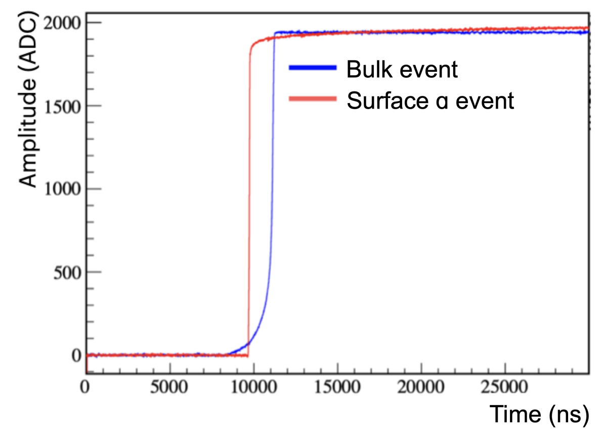
(b)

Figure 2: (a) Pulse shape plot of single-site events (top) and multi-site events (bottom). The black line shows the raw waveform in ADC counts and the red line shows the waveform in current amplitude. (b) Illustration of waveforms from surface alpha event and bulk event.

Most $0\nu\beta\beta$ events are single-site events which deposit all of their charge in a single location of $<$1 mm linear dimension in detector. This type of event appears in a Majorana Demonstrator detector as a waveform with a single sharply-rising step, as indicated by the black trace in the top panel of Figure 2(a). Since the waveform itself is the integrated ionized charge collected from an energy deposition in the detector, the derivative of the waveform (red traces in the same panel) is effectively the current induced as charges drift towards the point contact. In the Majorana Demonstrator, two major background sources are multi-site events and surface-alpha events. If charge is deposited at multiple locations within the crystal, the drift times may differ up to $\sim$1 $\mu$s, resulting in a waveform with multiple steps as shown in the bottom panel of Figure 2(a). This leads to a current pulse with a smaller maximum value than that of a single-site event with the same energy. Based on this first principle, we designed the current amplitude vs. energy (AvsE) described in Reference [38]. The current amplitude is estimated by a linear fit to a smaller range of the waveform. Cutting on the energy-normalized current amplitude (or AvsE) leads to efficient multi-site event rejection. In the standard Majorana analysis, we select events from a dedicated AvsE range by applying both low and high AvsE cuts.

The other major source of backgrounds at $Q_{\beta\beta}$  is from the alpha particles impacting the passivated surface and p+ contact surfaces of detectors. Prior to the most recent Majorana Demonstrator data release [33], this background source was rejected entirely using the first principle of the “delayed charge recovery” effect [39]. Based on the characteristics of alpha interactions, it appears that charge mobility is drastically reduced on or near the passivated surface. Therefore, a fraction of the charge from these interactions is slowly released on the timescale of waveform digitization, leading to a measurable increase in the slope of the waveform tail. The delayed charge recovery effect lowers the peak amplitude and as shown in Figure 2(b) results in a slowly rising tail slope that distinguishes this event from a bulk event at the same energy. The delayed charge recovery (DCR) cut tags events with larger tail slopes to efficiently reject surface alphas.

At a later stage of the standard Majorana analysis, a novel analysis cut based on the first principles of late charge (LQ) was developed. The LQ cut probes the top of the rising edge of the waveform to identify delayed charge collection on $~{}\sim 1\mu s$ timescale. It efficiently eliminates events in the transition layer and an additional population of near-point-contact events.

The final Majorana Demonstrator standard analysis is described in Reference [33]. The standard Majorana analysis for the PPC detectors is developed with the Germanium Analysis Toolkit (GAT), and is thus referred to as the “GAT analysis”. The standard Majorana analysis for the ICPC detectors is developed independently from GAT, and is referred to as the “ORNL analysis”. Both the GAT and ORNL analyses contain independently developed pulse shape discrimination (PSD) cuts derived from the first principles of HPGe detector charge collection: current amplitude versus energy, the delayed charge recovery effect, as well as the late charge effect. In this paper, we denote those cuts as GAT AvsE/DCR/LQ cut and ORNL AvsE/DCR/LQ cut, respectively.

During the development of the standard Majorana analysis, we observed that the PSD parameters vary with the length of time it takes the charges to drift to the p+ electrode, defined as drift-time, due to well-understood charge cloud diffusion and bulk charge trapping effects. Therefore, a drift-time correction was made to correct for this correlation. In the following text, we will use the terms “standard AvsE/DCR/LQ” to refer to the GAT analysis for PPC detectors and ORNL analysis for ICPC detectors, respectively. Additionally, we extracted the raw AvsE and raw DCR parameters, which are preliminary versions of standard AvsE/DCR thereby not directly used by the standard Majorana analysis. The raw parameters are generated under the GAT framework with a detector- and run-wise energy calibration applied. However, the raw parameters are not drift-time corrected, thus underperforming the standard Majorana analysis parameters. In this work, we decided to use the raw AvsE/DCR parameters to train the BDTs, and then compare the training results to the standard Majorana analysis parameters. The LQ parameters are introduced at a later stage of the standard Majorana analysis, thus we decided not to incorporate it to train the machine learning analysis. However, we did include LQ when comparing the two analyses in Section V.3.

III Data Pipeline

We collected both a signal and a background dataset to train the BDT. The signal dataset should be representative of the signal ($0\nu\beta\beta$ events in our case), and the background dataset should represent the proper background to reject. Before creating signal and background datasets from the Majorana data, a standard suite of cuts is applied: periods of high noise associated with liquid nitrogen fills or unstable operation are removed; non-physical waveforms, pileup waveforms, and pulser events are then removed by data cleaning cuts; and finally events in which multiple germanium detectors are triggered are removed. We particularly avoided the usage of high-level selection cuts, such as standard AvsE/DCR/LQ, since the tuning and validation of these cuts can be time-consuming. Decoupling from these cuts allows a fast-track application of this model on newly-taken data from multiple detectors. We then chose events in the double escape peak (DEP) from ²²⁸Th calibration data as the signal dataset. The DEP events are pair production events where both gammas have successfully escaped from the detector, thus mostly single-site events. An energy cut of $1592.5\pm 2.5$ keV is applied to select DEP events. Monte Carlo simulations including X-ray excitations and bremsstrahlung predict the events under DEP selection criteria to be 90% single-site with 10% multi-site impurities.

Table 1: List of input features to the MSBDT and the $\alpha$BDT. Cat. stands for categorical and Cont. stands for continuous.

Features	Type	Description
detType	Cat.	detector type: enriched PPC or ICPC
channel	Cat.	detector DAQ channel
tDrift	Cont.	drift time from the start of the rise to 99% waveform amplitude
tDrift50	Cont.	drift time from the start of the rise to 50% waveform amplitude
AvsE	Cont.	raw A. vs E, pulse shape parameter for multi-site event rejection[38, 33]
DCR	Cont.	raw DCR, pulse shape parameter for alpha event rejection [39, 33]
noise	Cont.	measuring 10-20MHz noise
DS	Cat.	data period the event belongs to, defined by run ranges

The background datasets for the MSBDT and the $\alpha$BDT are selected separately. For MSBDT, we select events under the single escape peak (SEP) of ²²⁸Th calibration data. The SEP events are pair production events where only one gamma has escaped from the detector. Although all SEP events are technically multi-site, if those sites occur at the isochrones of equal drift-time, they will reach the point contact at roughly the same time. In that case, the time difference between the two sites is smaller than the detector’s timing resolution, resulting in an apparently single-site waveform even though more than one energy deposition has occurred. These events are the impurities to the background dataset. An energy cut of $2103.5\pm 2.5$ keV is applied to select these events.

For the $\alpha$BDT, since the major alpha backgrounds are energy-degraded alpha events from the continuum, we have to select training data from a broader spectrum. We first select high energy alpha events by collecting events above 2615 keV in background runs. This sample is expected to have some contamination from high energy gamma events, originating from the decay of cosmogenically- and neutron-induced isotopes and uranium/thorium chain. We then select low energy alpha events by collecting the DCR tagged background events in a 1000-2615 keV energy range. In this way, a total of 723 high energy alpha and 2,839 low energy alpha events are selected.

After event selection, we extract 8 features from every event. The names and descriptions of these parameters are listed in Table 1. AvsE and DCR are dedicated pulse shape parameters for multi-site/alpha rejection respectively. Other parameters are added to probe their multivariate correlations with AvsE/DCR and to each other. For example, adding the channel parameter will allow the model to perform detector-wise tuning; adding tDrift and tDrift50 will allow the model to perform a drift-time correction, and our noise parameter allows us to look for correlations during noisy periods in the data. Among all features in Table 1, some features are continuous and some features are categorical. BDTs naturally handle both types of feature in the structure of the tree, allowing us to train on all detectors from all run periods simultaneously.

III.1 Data Augmentation

The data we selected above are highly imbalanced. First of all, only about 4% of data points are provided by ICPC detectors while the rest are from PPC detectors. Secondly, only 3,562 $\alpha$ events are collected compared to  600,000 DEP events in $\alpha$BDT training. This forms a typical long tail distribution where the head class contains most of the events and the tail class contains only a minimal proportion. If a BDT is trained with such an imbalanced dataset, it will be heavily biased towards the ample head class while ignoring the scarce tail class. We fix this issue by performing data augmentation.

Data augmentation refers to algorithms that generate synthetic data points to boost the population of the tail class for training purposes. We employ it to boost the population of both ICPC detector events and surface alpha events. The input dataset contains 8 features per event, 3 of which are categorical features. A Synthetic Minority Over-sampling TEchnique - Nominal and Continuous (SMOTE-NC) [40] algorithm is adopted for data augmentation. SMOTE-NC generates synthesized data by randomly interpolating between datapoints and its nearest neighbors. It works well on low dimensional data with both continuous and categorical features. It is first applied to all 3 datasets (DEP, SEP and alpha) to boost the population of ICPC events by a factor of $\sim$50, then applied again on the alpha dataset to boost the population of alpha events by a factor of $\sim$115. We refer to the events directly collected from detectors as genuine events and the events from data augmentation as augmented events. The augmented events are only used for training; model evaluation that will be discussed in Section V is based on genuine events.

III.2 Distribution Matching

While building our BDT models, we want them to look at the correlations of features instead of single features, unless that single feature is the first-principle feature as discussed in Section II. The first-principle feature—that is AvsE for MSBDT or DCR for $\alpha$BDT—is designed to fulfill the same background rejection goal as the BDT model. We do not expect features other than the first-principle feature to contribute to the classification independently, but they can contribute through their correlations with the first-principle feature or other features. Undesirable behavior arises when other parameters are allowed to contribute independently to classification. For example, if a given channel in the MSBDT training dataset is accidentally biased to contain 50% more signals than backgrounds, the BDT will “remember” this bias and tend to classify events in this channel as signal regardless of the rest of the features. If we then validate the BDT on another out-of-sample, unbiased dataset, the classification performance on this channel will be suppressed. This phenomenon is referred to as overfitting.

Figure 3: Distribution matching of the tDrift feature in input data.

To avoid this kind of overfitting, we carried out a process called “distribution matching” on 6 out of 8 secondary features. Figure 3 shows the distribution matching effect on the tDrift feature. The distribution of each secondary feature is first put into a histogram with predefined bin width. Then for every bin in the histogram, we randomly sample without replacement the same number of events from the signal and background datasets. This will reduce the size of both signal and background datasets to the same amount. Eventually, the sampled events are aggregated into a new signal/background dataset. We leave the first-principle feature—AvsE for MSBDT and DCR for $\alpha$BDT—unmatched because we expect them to follow different distributions between the signal and background dataset. The detType feature is not matched either since it overlaps with the channel feature. After distribution matching, the signal/background dataset spectrum will exhibit the same spectrum shape over matched secondary features. Distribution matching only affects the training dataset. The performance of trained BDT is evaluated on both DEP/SEP datasets and a flat Compton Continuum(CC) dataset, as described in Section V.3 and Table 2.

In summary, the data pipeline for the MSBDT contains the following steps: we first select ²²⁸Th DEP events as the signal dataset and ²²⁸Th SEP events as the background dataset; we then extract eight features as described in Table 1 for every event in both datasets; we then perform data augmentation to generate augmented ICPC events; lastly, we perform distribution matching on all features except AvsE and detType. The data pipeline of the $\alpha$BDT  contains the following steps: we first select ²²⁸Th DEP events as the signal dataset, and aggregate both low- and high-energy alphas to form the genuine alpha dataset; we then extract eight features; perform data augmentation to generate augmented ICPC detector events and alpha events as the background dataset; lastly, we perform distribution matching on all features except DCR and detType.

IV Boosted Decision Tree

The decision tree (DT) model produces classification decisions by making a series of binary choices. This features allow decision tree to naturally handle both continuous and categorical dataset, without the need of additional structures such as one-hot encoding. Boosting algorithms allow the machine to generate many decision trees iteratively to form a classification “committee”. After training the m^th decision tree, the classification committee containing the first through m^th trees is denoted $T_{m}(x_{i})$. The dataset can be described as $\{x_{i},y_{i}\}_{i=0}^{k}$, where $x_{i}$ is the input event, $y_{i}$ is the label and k is the number of events. The dataset is modified according to the output of $T_{m}(x_{i})$. The modified dataset is then fed into $T_{m+1}(x_{i})$ for training. The way the dataset is modified for each iteration defines the boosting algorithm type. In this work, the BDT model is trained using the LightGBM package [41]. LightGBM adopts a gradient boosting algorithm [42] to grow decision trees. First, a binary cross-entropy loss function $L(y_{i},T_{m}(x_{i}))$ is defined for the classification task, where $y_{i}$ is the event label. Then for each data point, we calculate the pseudo-residual $r_{im}$:

$$r_{im}=-\frac{\partial L(y_{i},T_{m}(x_{i}))}{\partial T_{m}(x_{i})}$$ (1)

$r_{im}$ is the negative gradient of the loss function with respect to the classification committee output at $x_{i}$. For each boosting iteration, the dataset is modified from $\{x_{i},y_{i}\}_{i=0}^{k}$ to $\{x_{i},r_{im}\}_{i=0}^{k}$, then a new decision tree $h_{m+1}(x)$ is fit to the modified dataset. The new decision tree is incorporated into the committee via the following equation:

$$T_{m+1}(x)=T_{m}(x)+\gamma_{m+1}h_{m+1}(x)$$ (2)

Where $\gamma_{m+1}$ is chosen to minimize the loss function by solving the following optimization problem:

$$\gamma_{m+1}=\operatorname*{arg\,min}_{\gamma}\sum_{i=0}^{k}L(y_{i},T_{m}(x_{i})+\gamma h_{m+1}(x_{i}))$$ (3)

The procedure above describes the mathematical formulation of BDT training. To train the BDT model, we first mix and shuffle the signal and background datasets. We then split the mixed dataset into training and validation datasets with an 80:20 ratio. The BDT models are trained on the training dataset. An early stopping algorithm will terminate the training process if the loss on the validation dataset does not decrease for a given number of iterations. The performance is quantified on a dedicated evaluation dataset which will be discussed later in Section V; the interpretability study is conducted on a customized interpretability dataset, which will be discussed later in Section VI.

LightGBM contains several highly customizable BDT models defined by collections of hyperparameters. Hyperparameters refer to parameters that do not change during training, such as the type of boosting algorithms, maximum number of trees to grow, number of early stopping iterations, and maximum number of leaves per tree. Some hyperparameters may greatly impact the metric, while other parameters may have minimal to no impact. All hyperparameters are searched simultaneously using Bayesian optimization to maximize the background rejection efficiencies at 90% signal acceptance [43].

V Result

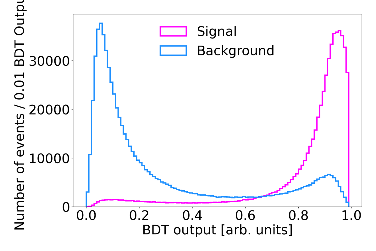
(a)

(b)

Figure 4: (a) MSBDT score distribution for signal and background events. (b) Background subtracted ROC curve for MSBDT classifier, AvsE corrected classifier and AvsE classifier. The ROC curve plots the true positive rate (TPR) vs. the false positive rate (FPR) of a binary classifier by placing the cutting threshold at every possible location. Larger area under ROC curve represents better classification performance. For both AvsE classifiers, only the traditional low AvsE cut are applied.

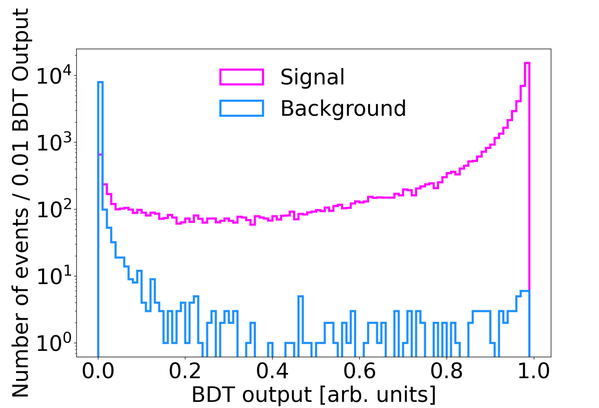
(a)

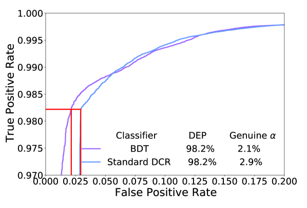
(b)

Figure 5: (a) $\alpha$BDT output distribution for signal and background events. (b) ROC curve for $\alpha$BDT classifier and standard DCR classifier.

After training, we evaluate the performance of both the MSBDT and the $\alpha$BDT. The trained BDT model takes the input of 8 features as described in Table 1, and outputs a single floating point number as the classification score between 0 and 1. A higher classification score indicates the input event is more signal-like and a lower classification score indicates the input event is more background-like. A cutting threshold is placed to accept signals and reject backgrounds. The selection criteria of the cutting threshold will be discussed in the following subsections. We also use the Receiver Operating Characteristic (ROC) [44] curve to gauge the classification performance of our models. The ROC curve plots the true positive rate (TPR) vs. the false positive rate (FPR) by placing the cutting threshold at every possible location. The fraction of area under the ROC curve (AUC) statistically describes the classification power of a binary classifier, in that larger AUC corresponds to better classification performance and smaller AUC corresponds to worse classification performance. For example, an AUC of 1 indicates perfect classification, and an AUC of 0.5 indicates no classification.

V.1 MSBDT Result

Events from the ²²⁸Th calibration data sets are used to test the MSBDT. The DEP events from 1590-1595  keV are used as the signal event sample, and the SEP events from 2101-2106 keV are used as the background event sample. The MSBDT score spectra for signal and background samples are illustrated in Figure 4(a). The signal and background peaks are well-separated, albeit with “misclassified” events under both peaks. Since both the signal and the background samples have impurities described in Section III, these events could be the impure events and thus being correctly classified.

Table 2: Table of survival fractions of signal and background events in each Majorana Demonstrator dataset. The signal and background event selection is defined in Section V.1 for MSBDT and Section V.2 for the $\alpha$BDT . The BDT cutting thresholds are selected so that they produce the same signal acceptance with the standard analyses. The AvsE corrected, DCR corrected and LQ parameters are adopted in the standard Majorana analysis. CC stands for the compton continuum (1989-2089 keV) events in ²²⁸Th calibration dataset, and BEW stands for the $0\nu\beta\beta$ background estimation window events (1950-2350 keV, excluding three gamma peaks) in the $0\nu\beta\beta$ search dataset. The survival numbers in BEW are calculated after joint cuts. The number in parentheses (last column of Row 11) is the survival number without the LQ cut.

Row	Dataset	DS0	DS1	DS2	DS3	DS4	DS5	DS5c	DS6	DS6c	DS7	DS8	DS8	All DS
Index	Detector Type	PPC	PPC	PPC	PPC	PPC	PPC	PPC	PPC	PPC	PPC	PPC	ICPC	(Expo. Weighted)
1	Exposure(kg $\cdot$ yr)	1.13	2.24	1.13	0.96	0.26	4.49	2.34	24.52	13.25	4.44	6.41	2.74	64.5
2	Single Site Signal (%)	90.3	89.8	88.6	89.9	89.4	89.1	87.4	89.4	89.8	89.7	89.7	88.7	89.5
3	MSBDT Bkg. (%)	5.62	5.85	5.01	5.71	6.31	5.95	5.70	5.73	5.58	4.57	6.41	5.76	5.71
4	Standard AvsE Bkg. (%)	6.13	6.29	5.93	5.31	5.48	6.24	6.51	6.25	6.39	6.00	6.78	6.17	6.25
5	MSBDT Cal. CC (%)	41.9	38.9	36.8	39.7	42.1	41.9	42.6	42.1	40.5	35.6	32.5	31.4	40.3
6	Standard AvsE Cal. CC (%)	43.1	42.9	41.5	41.0	42.1	42.0	41.6	42.3	42.7	42.1	43.3	35.0	42.3
7	Bulk Event Signal (%)	97.9	97.8	98.1	98.9	98.0	97.8	97.8	98.5	98.3	98.5	98.6	97.6	98.2
8	$\alpha$BDT Bkg. (%)	0.4	1.4	2.1	0.8	1.2	3.8	3.4	1.6	1.9	3.5	4.7	8.1	2.1
9	Standard DCR Bkg. (%)	1.7	1.9	2.8	3.9	0.0	2.9	5.7	2.6	3.1	5.4	2.8	0.8	2.9
10	BDT $0\nu\beta\beta$ BEW (#)	11	6	2	0	0	8	6	66	23	20	19	3	164
11	Standard $0\nu\beta\beta$ BEW (#)	11	4	1	0	0	9	5	58	20	17	24	4	153 (168)

The ROC curves of MSBDT, standard AvsE, and raw AvsE are shown in Figure 4(b). At each cutting location, the baseline subtraction and uncertainty evaluation are then performed in the same way as in Reference [38]. To set the MSBDT cutting threshold, we first apply the standard AvsE cut—that is, AvsE $>-1.0$—to the evaluation dataset. This cut leads to a TPR of 89.6%, shown as the horizontal magenta line in Figure 4(b). Next, the BDT cutting threshold and raw AvsE cutting threshold are selected to reach the same TPR as the standard AvsE. At this level of TPR, the survival fraction of background samples of the raw AvsE, the standard AvsE and MSBDT are 7.40%, 6.25%, and 5.71%, respectively. The standard AvsE leverages the drift-time correlations to reject 16.3% of SEP events that the raw AvsE accepts. MSBDT leverages additional multivariate correlations to reject a further 8.6% of SEP events that the standard AvsE accepts.

Rows 2-4 in Table 2 compares the performance of the MSBDT and the standard AvsE for each Majorana dataset. For most datasets, the MSBDT outperforms the standard AvsE on selected data samples. This demonstrates the ability of our BDTs to self-discover the drift-time corrections and other possible feature correlations to improve background rejection performance. Meanwhile, introducing DS, channel, and detType as categorical features allows the machine to perform detector- and run-level tuning without explicitly programming. However, the background data samples described above are only good representations of the true background dataset; the deviation from true background dataset could come from energy  (DEP energy vs. $Q_{\beta\beta}$ energy) and subtle differences in the intra-detector distribution of event positions. Therefore, additional data samples are collected to examine model performance near the true energy region of interest of $0\nu\beta\beta$ decay. These data samples—denoted as Calibration Compton continuum (Cal. CC) samples, contain all events between 1989 and 2089 keV from the ²²⁸Th calibration runs. Only 40.3% of Cal. CC samples survive MSBDT while 42.3% survive standard AvsE as shown in Row 5-6, Table 2.

V.2 $\alpha$BDT Result

Events from the ²²⁸Th calibration data sets and the $0\nu\beta\beta$ search data sets are used to test the $\alpha$BDT. All ²²⁸Th calibration events between 1000 keV and 2380 keV that pass the standard AvsE cut are selected as the signal samples, and the collection of genuine alpha events are selected as the background samples. The $\alpha$BDT output distribution of signal and background datasets are shown in Figure 5(a). Based on the plot, the background dataset is highly concentrated near 0.0 BDT score, indicating an excellent alpha tagging efficiency of the $\alpha$BDT. Meanwhile, the signal dataset spans the entire range, but most events are still concentrated near 1.0 $\alpha$BDT output.

The ROC curves of the $\alpha$BDT and the standard DCR parameter are shown in Figure  5(b). A cutting threshold is set at the horizontal red line to accept 98.2% of signal events. This acceptance matches the standard DCR acceptance in the standard Majorana analysis. At this cutting threshold, the DCR corrected analysis has 2.9% background acceptance, while the $\alpha$BDT only accepts 2.1% of surface alpha events. As mentioned in Section III, low energy genuine alpha are DCR tagged background events between 1000 keV and 2615 keV. Therefore, when evaluating the performance of the standard DCR cut, 100% of low energy genuine alpha will be manifestly removed. Given the fact that standard DCR is “cheating” on low energy alpha rejection, the $\alpha$BDT  still outperforms standard DCR by rejecting 27.6% of genuine alpha events that standard DCR accepts.

V.3 Comparison to Standard Majorana Analysis

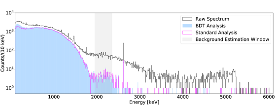
Figure 6: Energy spectrum of the standard Majorana analysis and the BDT analysis with 64.5$\pm$0.9 kg exposure, a good agreement is reached within the background estimation window. The low energy discrepancy between two analyses was mainly due to the LQ cut.

The background index of the standard Majorana analysis is evaluated in the $0\nu\beta\beta$ Background Estimation Window ($0\nu\beta\beta$ BEW). The $0\nu\beta\beta$ BEW samples are collected from 1950 to 2350 keV, excluding $\pm$5 keV region around the 2039 keV $Q_{\beta\beta}$ value and three gamma peaks at 2103 keV, 2118 keV and 2204 keV. Based on simulations, the background rate is expected to be flat after the exclusion. Both BDTs are applied to produce a number of survival events for $0\nu\beta\beta$ BEW in each dataset, which can be compared to the number of survival events for each dataset after applying the suites of standard Majorana analysis cuts: the standard AvsE cut, the high AvsE cut, the DCR cut, and the LQ cut. Note that neither the LQ feature nor the transition layer events are included in the BDT training process; thus, the BDT analysis will not be sensitive to these events. Given this “unfair” condition, the BDT analysis still manages to match and, in some datasets, outperform the standard Majorana analysis. The total number of $0\nu\beta\beta$ BEW survival events for BDT/standard Majorana analysis are 164 and 153 [33], indicating consistency between the two. As a comparison, standard Majorana analysis without LQ cut allows 168 events to remain in the $0\nu\beta\beta$ BEW. Figure 6 shows the comparison between the two analyses over the entire energy range. The two analyses agrees well except in the low energy region, where the standard Majorana analysis cuts more aggressively. This discrepancy is mainly subject to the the LQ cut, and the applicability of LQ at low energy is still under investigation. Therefore, these agreements show that the BDT analysis can start from raw parameters and tune them to match a highly optimized analysis.

V.4 ICPC Detectors

For the ICPC detectors, the trained BDT model takes the raw parameters as input and compares the output BDT score to the ORNL analysis parameters. This leads to additional challenges since the raw parameters are developed with GAT while the ORNL parameters are independently developed and customized for ICPC detectors. In this analysis, we use the raw parameters as inputs to train the BDT models to reach or exceed the background rejection performance of the ORNL analysis. This means that the BDT must perform multivariate corrections and account for the technical differences between two independently developed analyses. The second-to-last column of Table 2 shows the model evaluation results on ICPC detectors. MSBDT outperforms the ORNL AvsE for multi-site event rejection, with a background survival fraction of only 5.76%, compared to 6.17% for the ORNL AvsE. It also makes a significant improvement over its primary input parameter, raw AvsE, which has a 25% background survival fraction (not shown in Table II). On the other hand, the $\alpha$BDT underperforms the ORNL DCR with a 8.1% genuine alpha survival fraction, compared to 0.8% for the ORNL DCR. However, the $\alpha$BDT still makes a significant improvement over its primary input parameter, raw DCR, which allows 18% of genuine alphas to survive (not shown in Table II). The BDT analyses account for the technical differences among independently developed analyses to simultaneously analyze different types of germanium detectors. Finally, the result of the BDT analyses indicate that the GAT analysis has the potential to reach the same level of performance on ICPC detectors under proper tuning.

VI Machine Interpretability

We demonstrated the BDT’s ability to outperform the standard Majorana analysis, but the source of additional classification power was not readily apparent. To identify these sources, a post facto machine interpretability study was performed on the trained MSBDT and $\alpha$BDT. This study used a coalitional game theory concept, Shapley value [45], to interpret the decision of a BDT. The Shapley value is defined as follows:

$$\phi_{i}(v)=\sum_{S\subseteq N/\{i\}}\frac{|S|!(n-|S|-1)!}{n!}(v(S\cup\{i\})-v(S))$$ (4)

$v$ is the characteristic function that maps a subset of players to a real number. $S$ represents a coalition of players without the player $i$. $N$ is the set of all players and $n$ is the size of that set. In this analysis, $v$ is the BDT model mapping input features to the BDT score. Each feature is a “player” of the game. $v(S\cup\{i\})-v(S)$ describes the difference in BDT score including/excluding feature $i$. This difference is summed over all coalitions S — that is, the possible combinations of all other features except $\{i\}$ — to produce the Shapley value for $i$. Therefore, the Shapley value in the context of a BDT represents each feature’s contribution to the final BDT score, assuming they work collaboratively.

The interpretability study was conducted using the SHAP package [24]. The underlying mechanism is analogous to a one-dimensional free body diagram [46]. SHAP assigns a Shapley value to each feature of the events to be interpreted. The Shapley value acts as a “force” to change the BDT score: a positive Shapley value pushes the BDT score toward a more signal-like score, while a negative Shapley value pushes the BDT score toward a more background-like score. After all “forces” are applied, the BDT reaches an equilibrium, and the equilibrium position is the BDT score of the input event. Therefore, if an event is classified as signal, the feature with the largest positive Shapley value will be the driving factor for this classification decision, while features with negative Shapley values suggest against the classification decision. An example force plot of a single Majorana Demonstrator event is shown in Figure 7(c). By investigating the Shapley values on designated datasets, we will understand the driving feature which leads to the additional classification power.

VI.1 Interpreting MSBDT

Figure 7(a) presents a summary plot to illustrate the feature importance of the MSBDT. To make this plot, we first randomly sampled 10,000 ²²⁸Th DEP events and 10,000 ²²⁸Th SEP events to form the interpretability dataset. The Shapley values are calculated for each event in the dataset, and the distribution of Shapley values with respect to each input feature is plotted in Figure 7(a). The shape of these distributions represents the importance of the given feature. An important feature exhibits a dumbbell shape, indicating this feature drives the decision by a large magnitude most of the time. A less important feature exhibits a spindle shape, indicating this feature outputs a near-zero Shapley value most of the time but occasionally drives the decision with a large amplitude. An irrelevant feature exhibits a vertical bar shape, indicating that this feature almost always outputs a Shapley value of 0. Figure 7(a) ranks the importance of features from top to bottom according to this rule. The most important feature is AvsE as we expected, and the second most important feature is channel. This means MSBDT’s classification power mainly comes from channel-wise calibration of AvsE. The least important feature is detType since it is redundant with channel. The importance ranking shown in Figure 7(a) can also be used for feature selection. In case the computation power is limited, low-importance features such as detType can be removed from the input. In this work, the BDT training takes less than one miunte on CPU. Therefore, low-importance features are kept since they do not seem to adversely affect the performance.

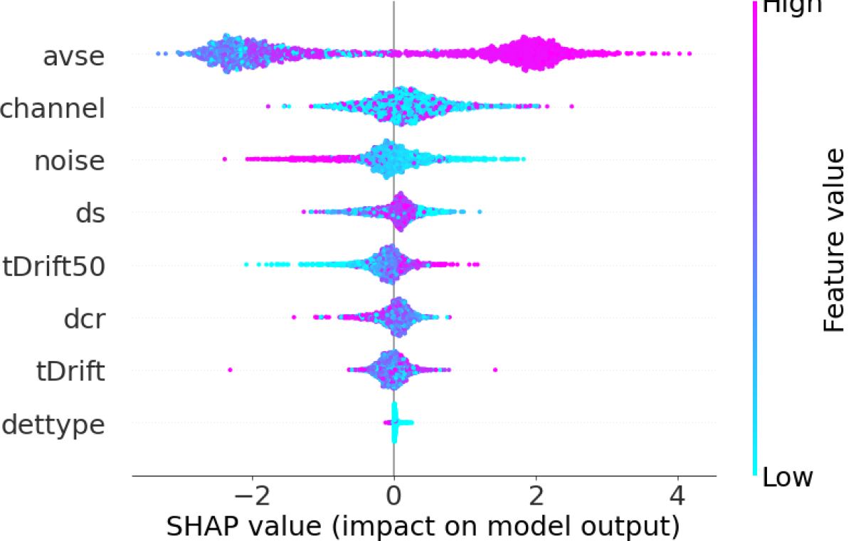
(a)

(b)

(c)

Figure 7: (a) Feature importance plot of the MSBDT. From top to bottom, the features are ranked from the most important to the least important. The color of each dot represents the Shapley value of each feature, normalized by the highest and lowest Shapley values of all input samples. (b) The scatter plot of raw AvsE vs. tDrift for outperforming events in a single detector in DS6. The color of each dot represents the sum of Shapley value assigned to both tDrift and tDrift50. Higher magnitude represents more important contributions from drift time. The green line represents a linear fit to the linear dependency of drift time. (c) Force plot of a single Majorana Demonstrator event denoted by the magenta diamond in (b). The Shapley value of AvsE and channel provides positive forces, while the Shapley value of tDrift, tDrift50, and dcr provides negative forces. The equilibrium position is at 0.34.

To further understand the classification power of MSBDT, especially the additional classification power compared to standard AvsE, we collected outperforming events from the interpretability dataset with two criteria:

• DEP events that MSBDT classifies as signal but raw AvsE classifies as background

• SEP events that MSBDT classifies as background but raw AvsE classifies as signal

Figure 7(b) shows the joint distribution of drift time and raw AvsE on a 2D scatter plot on outperforming events. To avoid smearing caused by different detectors or different datasets, only outperforming events from a single detector in DS6 are shown. The color of each dot indicates the summed Shapley value of tDrift and tDrift50. Two types of drift time dependencies are observed on raw AvsE: a linear dependency appears on the raw AvsE for large drift time events, and a non-linear dependency on low drift time events. In the standard Majorana analysis, the linear dependence is corrected through a detector-by-detector drift time correction as discussed in Section II. From the MSBDT’s perspective, the BDT assigns a positive Shapley value on drift time to reproduce the drift time correction: although the linear dependency leads to lower-than-usual AvsE at large drift time, the MSBDT successfully captures this dependency and produces a positive Shapley value to compensate for this effect. This is equivalent to the drift-time correction in standard Majorana analysis. Without explicit programming, the MSBDT independently learns these correlations from data and leverages them to further improve background rejection performance as expected.

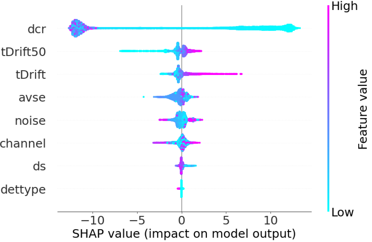
(a)

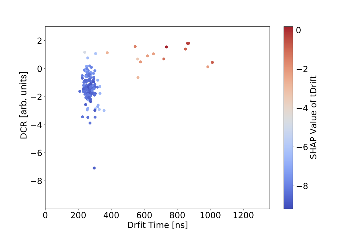
(b)

Figure 8: (a) Feature importance plot of the $\alpha$BDT. (b) The scatter plot of raw DCR vs. tDrift for all outperforming genunie alpha events. The color of each dot represents the sum of Shapley value assigned to both tDrift and tDrift50. Higher magnitude represents more important contributions from drift time.

The non-linear dependency happens primarily on events with drift time below 400 ns. These events happen near the point-contact and drift almost immediately to it. As shown in Figure 7(b), these fast-drifting events possess excessively high AvsE and will be classified as signals even if the waveform is multi-site. In the standard Majorana analysis, we use the high AvsE cut and the LQ cut to remove these events near the point-contact. In this analysis, the MSBDT assigns a negative Shapley value according to the drift time to compensate for the higher-than-usual AvsE values. To demonstrate this, we selected a single event from this region (the magenta diamond on Figure 7(b)) and showed its Shapley forces in Figure 7(c). Although the excessively high AvsE produces an overwhelmingly positive force, MSBDT recognizes the non-linear drift time dependency and assigns negative forces to tDrift and tDrift50 to counteract the positive force. The equilibrium position is at 0.34, which falls below the cutting threshold of MSBDT. Therefore, this event is rejected by MSBDT but accepted by standard AvsE. Without explicit programming, the MSBDT learns the linear and non-linear correlation from data and handles them correctly to produce better background tagging efficiency.

VI.2 Interpreting $\alpha$BDT

We used a similar approach to interpret the $\alpha$BDT. Since there are only 3,562 genuine alpha events, we collected all the genuine alpha events as backgrounds and 3,562 randomly sampled ²²⁸Th DEP events as signals to form the interpretability dataset. The summary plot is shown in Figure 8(a). As expected, raw DCR is the most important feature in making a classification decision. tDrift50 is the second most important feature, indicating that the $\alpha$BDT is mainly performing a drift-time correction on raw DCR to enhance its classification power. Similar to the MSBDT, detType is the least important feature since it is redundant with channel.

Outperforming events are collected from the interpretability dataset to understand the additional classification power of the $\alpha$BDT. Since the signal sacrifice of the $\alpha$BDT and DCR is negligible, the outperforming dataset is defined as genuine alpha events rejected by the $\alpha$BDT but accepted by the standard DCR. Figure 8(b) shows the joint distribution of drift time and standard DCR on a 2D scatter plot on outperforming events. These events form a cluster near a drift time of 200 ns, indicating that they are surface alpha events near the point contact. After creation, these events drift to the point contact almost immediately, leaving almost no delayed charge on the passivated surface thus violating the first principle of the DCR cut. However, the fast-drifting nature allows the $\alpha$BDT to efficiently tag these events based on their drift-time, thus outperforming the traditional analysis. As $\alpha$BDT interpretability study revealed the importance of these backgrounds, a dedicated high AvsE cut is introduced into the standard Majorana analysis to reject them. High AvsE turns out to also reject multisite event near the point contact as we discussed in Section VI.1.

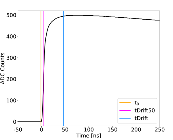
Figure 9: A typical surface alpha event waveform (black) near the point-contact of Majorana PPC detector. t₀ is the start of charge deposition. The time interval of tDrift50 and tDrift features are shown.

The interpretability study also shows that tDrift50 is more important in the $\alpha$BDT model than tDrift. This can be explained by the difference between the calculation of these two parameters. A typical outperforming event is shown in Figure 9. When a surface alpha event happens near the point-contact, the charge deposition starts almost immediately, leading to a sharp rising edge of the waveform. On the other hand, the passivated surface reduces the drift speed of charges comparatively further away from the point-contact. This effect delays the completion of charge deposition, leading to a rounded top of the waveform. Since tDrift is calculated from the the start of the rise to the time when the waveform reaches 99% of its maximum amplitude, the rounded-top structure significantly increases the value of tDrift, allowing it to appear as a slowly drifting event, thus escape the low drift-time/high AvsE cut. However, tDrift50 is immune to the rounded-top structure since it is caluclated only up to 50% of the waveform amplitude. The interpretability study suggests that a tDrift50-based cut could be developed to further benefit the alpha rejection in future first-principle analyses.

The interpretability study allows machine learning analysis to unveil physics in germanium detectors. Leveraging multivariate correlations and automatic categorization, the BDT was able to outperform individual PSD parameters and match both the GAT and the ORNL analyses, as discussed in Section V with less detector-by-detector calibration. Furthermore, the interpretability study leverages the additional classification power to reveal the importance of new background categories. This eventually led to the implementation of a high AvsE cut in the standard Majorana analysis and suggests a new direction for future improvement. The reciprocal relationship between the machine learning analysis and the traditional, first-principle analysis revealed by the interpretability study, demonstrates that an interpretable machine learning analysis can not only outperform but also benefit the traditional analysis.

VII conclusion

In this work, we have presented the first machine learning analysis for the Majorana Demonstrator; this is also the first interpretable machine learning analysis of any germanium detector experiment. This analysis contains two parts: learning from the data to improve background rejections and learning from the machine to understand classification power. Leveraging gradient boosted decision trees and data augmentation, this analysis outperforms the the individual PSD parameters and match the overall results of the highly optimized standard Majorana analysis [33]. Learning from data also closes the gap between two independently developed analyses applied to different types of detectors.

For the first time in the field, a thorough machine interpretability study is conducted, leveraging the Shapley value in coalitional game theory. This study not only justifies BDT’s capability to capture multivariate correlations but also to independently discover new background categories to reveal its importance. The machine learning analysis and the standard Majorana analysis established a reciprocal relationship through the interpretability study. Since BDT model is widely used in the particle and nuclear physics community [47, 48, 49, 50, 51, 52, 53], this work provides a template for interpreting the BDT model to gain more physical insight and even make new scientific discovery.

This work has focused on developing and interpreting the first machine learning analysis for Majorana Demonstrator. The data-driven nature of this analysis allows a straightforward generalization to different germanium detector experiments, especially the next-generation tonne-scale experiment LEGEND-1000 [23]. Given the large number of detectors, detector- and run-level tuning may be time-consuming in LEGEND. In that case, the BDT’s ability to simultaneously train on all detectors would be highly beneficial. Furthermore, the interpretability study allows us to unravel the black-box nature of machine learning models to reveal underlying physics and independently discover new background categories without explicit programming. We intend to apply this model to LEGEND data, which could enable improvements in background rejection, and possibly help us gain a more nuanced understanding of the detector performance. Our future work involves using more powerful and versatile machine learning models such as recurrent neural network (RNN). RNN can be trained directly on the Demonstrator’s waveform, which opens up an entirely new avenue for more machine learning applications.