Orbital and dynamical analysis of the system around HR 8799.

Abstract

Context. HR 8799 is a young planetary system composed of four planets and a double debris belt. Being the first multi-planetary system discovered with the direct imaging technique, it has been observed extensively since 1998. This wide baseline of astrometric measurements, counting over 50 observations in 20 years, permits a detailed orbital and dynamical analysis of the system.

Aims. To explore the orbital parameters of the planets, their dynamical history, and the planet-to-disk interaction, we made follow-up observations of the system during the VLT/SPHERE guaranteed time observation program. We obtained 21 observations, most of them in favorable conditions. In addition, we observed HR 8799 with the instrument LUCI at the Large Binocular Telescope (LBT).

Methods. All the observations were reduced with state-of-the-art algorithms implemented to apply the spectral and angular differential imaging method. We re-reduced the SPHERE data obtained during the commissioning of the instrument and in three open-time programs to have homogeneous astrometry. The precise position of the four planets with respect to the host star was calculated by exploiting the fake negative companions method. We obtained an astrometric precision of the order of 6 mas in the worst case and 1 mas in the best case. To improve the orbital fitting, we also took into account all of the astrometric data available in the literature. From the photometric measurements obtained in different wavelengths, we estimated the masses of the planets following the evolutionary models.

Results. We obtained updated parameters for the orbits with the assumption of coplanarity, relatively small eccentricities, and periods very close to the 2:1 resonance. We also refined the dynamical mass of each planet and the parallax of the system (24.49 $\pm$ 0.07 mas), which overlap with the recent GAIA eDR3/DR3 estimate. Hydrodynamical simulations suggest that inward migration of the planets caused by the interaction with the disk might be responsible for the planets being locked in resonance. We also conducted detailed $N$-body simulations indicating possible positions of a putative fifth innermost planet with a mass below the present detection limits of $\simeq 3$ $M_{\mathrm{Jup}}$.

1 Introduction

Among the exoplanets discovered with the high-contrast imaging technique (e.g., Chauvin et al. 2004; Lagrange et al. 2010; Rameau et al. 2013; Keppler et al. 2018; Bohn et al. 2021), the system around HR 8799 is undoubtedly one of the most interesting. This is mainly because HR 8799 hosts a greater number of planets detected with high-contrast imaging than any other system, only three systems that host two planets were detected: PDS 70 (Keppler et al. 2018; Haffert et al. 2019), TYC 8998-760-1 (Bohn et al. 2020), and $\beta$ Pic (Lagrange et al. 2010; Nowak et al. 2020). HR 8799 is a perfect laboratory with which to study dynamical interaction in young planetary systems, with its four planets (HR 8799 bcde; Marois et al. 2008, 2010) and a double debris belt (see, e.g., Su et al. 2009; Hughes et al. 2011; Matthews et al. 2014; Booth et al. 2016; Faramaz et al. 2021). The host star HR 8799 is a young ($\sim$ 42 Myr, Hinz et al. 2010; Zuckerman et al. 2011; Bell et al. 2015), $\gamma$ Dor-type variable star (Gray & Kaye 1999) with $\lambda$ Boo-like abundance patterns. The mass of the star is 1.47${}^{+0.12}_{-0.17}$ $M_{\odot}$ (Sepulveda & Bowler 2022) and its distance is 40.88 $\pm$ 0.08 pc from GAIA measurements (Gaia Collaboration 2020).

This system is an optimal target for high-contrast imaging observations, as its four planets are easily detectable with state-of-the-art imagers; their contrasts are about 2–8 $\times$ 10^-6; and the separation of the closest planet HR 8799 e is $\sim$ 390 mas, which is further than the inner working angle of most current instruments designed for direct imaging. For these reasons, the system has been observed dozens of times starting from 1998, with different instruments, wavelengths, and configurations. Thanks to this rich pool of archival data, HR 8799 can be studied in detail from an astrometric point of view, being the only multi-planetary system for which there are tens of astrometric data points on a baseline of more than 20 years. These measurements began with uncertainties of $\sim$ 20 mas, but have since reached unprecedented precision of below a milliarcsecond (0.1–0.2 mas) with optical interferometry (Gravity Collaboration et al. 2019).

Works regarding the analysis of the dynamical interaction of the four planets have been presented; most of these agree on the near coplanarity of the planets, and that they are locked in a 1:2:4:8 resonance, (see, e.g., Fabrycky & Murray-Clay 2010; Esposito et al. 2013; Konopacky et al. 2016; Zurlo et al. 2016; Wang et al. 2018; Gravity Collaboration et al. 2019; Goździewski & Migaszewski 2020). From the age of the system and the luminosity of the planets, evolutionary hot-start models derive masses of around 5–7 $M_{\mathrm{Jup}}$ (Marois et al. 2010; Currie et al. 2011; Sudol & Haghighipour 2012). These masses are compatible with the dynamical studies because small masses help the orbits to remain stable (e.g., Wang et al. 2018). On the other hand, Brandt et al. (2021) found a dynamical mass for the innermost planet HR 8799 e of 9.6${}^{+1.9}_{-1.8}$ $M_{\mathrm{Jup}}$ assuming that planets c, d, and e share the same mass within $\sim$ 20%. This result is 2 $M_{\mathrm{Jup}}$ higher than the prediction from the evolutionary models.

In this paper, we present all the astrometric measurements obtained during the whole guaranteed time observation (GTO) of VLT/SPHERE for HR 8799 bcde. Ad hoc observations were designed for the orbital follow-up of the four planets; HR 8799 was observed 21 times in total with SPHERE, and only four observations were rejected based on quality criteria. To complement the SPHERE measurement, we obtained one astrometric epoch with the instrument LUCI, installed at the LBT. This instrument observed HR 8799 as part of the commissioning phase of the new adaptive optics (AO) system. With a total of 18 epochs and the addition of all the astrometric measurements available in the literature (69 astrometric epochs in total), we performed the dynamical analysis of the system and the planet-to-disk interaction.

The outline of the paper is as follows: in Sect. 2, we present SPHERE and LUCI observations; in Sect. 3, we describe the reduction methods applied and the astrometric results that we obtained. In Sect. 4 we present the astrometric fitting for the four planets of HR 8799 and in Sect. 5 a possible interpretation of the history of the system. We also explored the possibility of the presence of a fifth planet, studying the planets–disk interaction (Sect. 6). We provide our conclusions in Sect. 7.

2 Observations

2.1 VLT/SPHERE

HR 8799 was observed several times during the SpHere INfrared survey for Exoplanets (SHINE, papers I, II, III; Desidera et al. 2021; Vigan et al. 2021; Langlois et al. 2021) during the GTO of VLT/SPHERE. The instrument SPHERE (Beuzit et al. 2019) is a planet finder equipped with an extreme AO system (SAXO; Fusco et al. 2006; Petit et al. 2014) to characterize substellar companions with high-contrast imaging. The near-infrared (NIR) arm includes the IR dual-band imager and spectrograph (IRDIS; Dohlen et al. 2008) and an integral field spectrograph (IFS; Claudi et al. 2008). During the observations, these two subsystems observed the target in parallel. HR 8799 was periodically observed for astrometric monitoring, the setup of the observations included three different filter pairs: IRDIS in $H2H3$ bands ($\lambda_{H2}$=1.593 $\mu$m, $\lambda_{H3}$=1.667 $\mu$m), in BB_H ($\lambda_{H}$=1.625 $\mu$m), and $K1K2$ bands ($\lambda_{K1}$=2.102 $\mu$m, $\lambda_{K2}$=2.255 $\mu$m). The coronagraph used for the shortest wavelengths was an apodized Lyot with a mask diameter of 185 mas and an inner working angle (IWA) of 0$\aas@@fstack{\prime\prime}$09 (see Boccaletti et al. 2008), while for $K1K2$ band the IWA is $\sim$ 0$\aas@@fstack{\prime\prime}$12. For a detailed description of the observing sequence, we refer the reader to Zurlo et al. (2014, 2016). In general, the working sequence includes an image of the off-axis star point spread function (PSF) for the flux calibration, a long coronagraphic sequence with the satellite spots (Langlois et al. 2013) mode, a second image of the stellar PSF, and the sky images. The waffle mode was used on purpose to assure maximum astrometric precision. The long waffle sequence was taken in pupil stabilized mode in order to apply the angular differential imaging (ADI; Marois et al. 2006) method. While IRDIS has a field of view of $\sim$11$\times$11 arcseconds, IFS is smaller (1.7^′′ $\times$1.7^′′), and only the two interior planets are visible. The SHINE observations are summarized in Table 1. For almost all the epochs, the observation was with IRDIS and IFS working in parallel. On a few occasions, IRDIS was used alone; these observations are marked in the table. We discarded data for time periods where the conditions did not permit a clear detection of the planets or there was a very poor signal-to-noise ratio (S/N). In particular, we rejected data from 2014 August 13 ( only IFS data were considered), 2014 December 08, 2015 July 29, and 2017 October 07. All the other observations are taken into account in this analysis.

Table 1: Summary of the observations of HR 8799 with IRDIS and IFS during SHINE.

UT date	Filter	$\Delta_{FoV}$ (∘)	S/NMin	S/NMax
2014-07-12	DB_H23	17	9	44
2014-08-13	BB_J	23	0	36
2014-12-04	BB_H	9	14	24
2014-12-05b	BB_H	8	11	25
2014-12-06b	BB_H	8	15	25
2014-12-08ab	BB_H	8	6	25
2015-07-03	DB_K12	18	12	75
2015-07-29ab	DB_J23	82	4	51
2015-07-30b	DB_K12	81	21	123
2015-09-27	DB_K12	24	10	71
2016-11-17	DB_H23	17	15	52
2017-06-14	DB_H23	19	14	67
2017-10-07a	BB_H	76	0	0
2017-10-11	BB_H	74	45	90
2017-10-12	BB_H	78	24	100
2018-06-18	DB_H23	34	20	78
2018-08-17	BB_H	73	29	57
2018-08-18	BB_H	73	42	106
2019-10-31	DB_K12	24	22	62
2019-11-01	DB_K12	54	38	114
2021-08-20	DB_H23	20	21	59

2.2 Large Binocular Telescope/SOUL-LUCI

HR 8799 was observed with LBT/SOUL-LUCI1 during its commissioning on night 2020 September 29. LUCI1 (Seifert et al. 2010) is a NIR spectro-imager that can work in a diffraction-limited regime with a sampling of 15 mas/pix. The AO correction is provided by SOUL (Pinna et al. 2019), the upgrade of the FLAO system (Esposito et al. 2010). During this observation, the SOUL system was correcting 500 modes with a rate of 1.7 kHz. No coronagraphic masks are available on LUCI, and therefore to avoid any saturation, HR 8799 was observed adopting a sub-windowing of 256$\times$256 pixels (corresponding to a field of view (FoV) of 3.84$\times$3.84^′′). In this way, we were able to set a minimum exposure time of 0.34 s. We observed this target in pupil stabilization mode with two narrow-band filters: FeII ($\lambda_{FeII}$=1.646 $\mu$m; $\Delta\lambda$=0.018 $\mu$m) and H2 ($\lambda_{H2}$=2.124 $\mu$m; $\Delta\lambda$=0.023 $\mu$m). The observations with the two filters were alternated during the whole sequence.

3 Data reduction

3.1 SPHERE

The reduction of the IRDIS data was carried out entirely with the Data Center (DC; Delorme et al. 2017) which uses the standard SPHERE pipeline SpeCal (Galicher et al. 2018). For the astrometric calibration, we used a true north orientation of -1.75 deg and a pixel scale value of 12.25 mas as reported in Maire et al. (2016). The reduction algorithm used by the DC for HR 8799 is the T-LOCI (Marois et al. 2014). To provide a homogeneous reduction of all the IRDIS data, we processed the observations presented in Zurlo et al. (2016) again, which were previously reduced with custom routines, which included seven epochs in 2014 (we excluded the sequence of 2014 August 13 for poor quality). The four epochs taken for variability monitoring —once per night (2014 December 4, 2014 December 5, 2014 December 6, 2014 December 8)— and presented in Apai et al. (2016) were reprocessed with the DC. As in Apai et al. (2016), we excluded the sequence of December 8 for poor conditions. In the same way, we used the DC to reduce the data from the variability monitoring of Biller et al. (2021), with observation dates: 2015 July 29, 2015 July 30, 2017 October 07, 2017 October 11, and 2017 October 12 (two epochs were excluded for poor quality), and 2018 August, 17-18. Finally, we re-processed the IRDIS data presented by Wahhaj et al. (2021) and taken on October 31, 2019, and November 1, 2019. In the DC, a “fake negative planets” (e.g., Zurlo et al. 2014, and references therein) algorithm is implemented to calculate the precise position of each planet with respect to the central star. A summary of all the SPHERE astrometric points, both from the SHINE survey and published observations presented in Zurlo et al. (2016), Apai et al. (2016), Biller et al. (2021), and Wahhaj et al. (2021) is listed in Table 2 (IRDIS) and 3 (IFS). We refer the reader to these latter publications for further information about the observing conditions. The results of the updated astrometry are also listed in Table LABEL:t:lite, together with all the other data from different instruments presented in the literature.

From the IRDIS photometry, we also estimated the mass of each planet using evolutionary models. In particular, we applied evolutionary models from Baraffe et al. (2003, 2015) to the IRDIS filters photometry. The age of the system used in this estimation is 42 Myr and the parallax is 24.46 $\pm$ 0.05 mas, as in GAIA EDR3. The error reported is the standard deviation between different epochs taken with the same filter. Results are listed in Table 4.

Table 2: List of astrometric points from IRDIS observations.

Date	Planet b	Planet c	Planet d	Planet e
	$\Delta$RA ; $\Delta$Dec (mas)	$\Delta$RA ; $\Delta$Dec (mas)	$\Delta$RA ; $\Delta$Dec (mas)	$\Delta$RA ; $\Delta$Dec (mas)
2014-07-12	1570 $\pm$ 3 ; 704 $\pm$ 3	-521 $\pm$ 3 ; 790 $\pm$ 9	-391 $\pm$ 2 ; -530 $\pm$ 2	-387 $\pm$ 2 ; -10 $\pm$ 3
2014-12-04	1574 $\pm$ 3 ; 701 $\pm$ 2	-514 $\pm$ 3 ; 798 $\pm$ 4	-399 $\pm$ 4 ; -525 $\pm$ 4	-389 $\pm$ 8 ; 11 $\pm$ 4
2014-12-05	1574 $\pm$ 4 ; 701 $\pm$ 3	-512 $\pm$ 3 ; 798 $\pm$ 4	-400 $\pm$ 4 ; -523 $\pm$ 4	-390 $\pm$ 7 ; 12 $\pm$ 4
2014-12-06	1573 $\pm$ 3 ; 701 $\pm$ 3	-512 $\pm$ 3 ; 797 $\pm$ 4	-403 $\pm$ 4 ; -524 $\pm$ 4	-383 $\pm$ 8 ; 11 $\pm$ 4
2015-07-03	1579 $\pm$ 1 ; 694 $\pm$ 1	-498 $\pm$ 1 ; 806 $\pm$ 1	-417 $\pm$ 1 ; -517 $\pm$ 1	-383 $\pm$ 9 ; 33 $\pm$ 5
2015-07-30	1580 $\pm$ 5 ; 689 $\pm$ 3	-495 $\pm$ 2 ; 806 $\pm$ 2	-419 $\pm$ 2 ; -516 $\pm$ 1	-386 $\pm$ 1 ; 36 $\pm$ 1
2015-09-27	1580 $\pm$ 1 ; 688 $\pm$ 1	-494 $\pm$ 1 ; 811 $\pm$ 1	-426 $\pm$ 1 ; -512 $\pm$ 1	-382 $\pm$ 9 ; 50 $\pm$ 5
2016-11-17	1589 $\pm$ 2 ; 666 $\pm$ 1	-464 $\pm$ 2 ; 824 $\pm$ 2	-454 $\pm$ 2 ; -490 $\pm$ 2	-378 $\pm$ 4 ; 90 $\pm$ 2
2017-06-14	1591 $\pm$ 1 ; 653 $\pm$ 1	-449 $\pm$ 1 ; 835 $\pm$ 1	-472 $\pm$ 2 ; -482 $\pm$ 2	-373 $\pm$ 3 ; 118 $\pm$ 2
2017-10-11	1595 $\pm$ 1 ; 647 $\pm$ 1	-441 $\pm$ 1 ; 839 $\pm$ 1	-480 $\pm$ 1 ; -477 $\pm$ 1	-369 $\pm$ 1 ; 128 $\pm$ 1
2017-10-12	1595 $\pm$ 1 ; 647 $\pm$ 1	-441 $\pm$ 1 ; 839 $\pm$ 1	-480 $\pm$ 1 ; -477 $\pm$ 1	-371 $\pm$ 2 ; 128 $\pm$ 2
2018-06-18	1601 $\pm$ 1 ; 635 $\pm$ 1	-424 $\pm$ 1 ; 848 $\pm$ 1	-497 $\pm$ 2 ; -463 $\pm$ 2	-358 $\pm$ 2 ; 156 $\pm$ 2
2018-08-17	1601 $\pm$ 2 ; 632 $\pm$ 3	-421 $\pm$ 1 ; 850 $\pm$ 1	-502 $\pm$ 1 ; -461 $\pm$ 1	-357 $\pm$ 1 ; 162 $\pm$ 2
2018-08-18	1600 $\pm$ 1 ; 632 $\pm$ 1	-421 $\pm$ 1 ; 851 $\pm$ 1	-502 $\pm$ 2 ; -458 $\pm$ 1	-358 $\pm$ 2 ; 163 $\pm$ 1
2019-10-31	1606 $\pm$ 2 ; 615 $\pm$ 2	-392 $\pm$ 2 ; 875 $\pm$ 2	-532 $\pm$ 3 ; -425 $\pm$ 2	-338 $\pm$ 2 ; 215 $\pm$ 2
2019-11-01	1611 $\pm$ 1 ; 611 $\pm$ 1	-388 $\pm$ 2 ; 870 $\pm$ 2	-530 $\pm$ 2 ; -430 $\pm$ 1	-335 $\pm$ 1 ; 210 $\pm$ 1
2021-08-20	1626 $\pm$ 1 ; 578 $\pm$ 2	-339 $\pm$ 2 ; 890 $\pm$ 2	-563 $\pm$ 2 ; -391 $\pm$ 2	-287 $\pm$ 4 ; 272 $\pm$ 2

Table 3: List of astrometric points from IFS observations.

Date	Planet d	Planet e
	$\Delta$RA ; $\Delta$Dec (mas)	$\Delta$RA ; $\Delta$Dec (mas)
2014-07-12	-400 $\pm$ 4 ; -512 $\pm$ 4	-389 $\pm$ 1 ; -22 $\pm$ 2
2014-08-13	-396 $\pm$ 1 ; -524 $\pm$ 1	-389 $\pm$ 1 ; -17 $\pm$ 2
2015-07-03	-424 $\pm$ 4 ; -509 $\pm$ 3	-391 $\pm$ 1 ; 33 $\pm$ 2
2015-09-27	-420 $\pm$ 4 ; -513 $\pm$ 4	-392 $\pm$ 1 ; 39 $\pm$ 3
2016-11-17	-464 $\pm$ 1 ; -486 $\pm$ 2	-382 $\pm$ 2 ; 94 $\pm$ 6
2017-06-14	-473 $\pm$ 2 ; -476 $\pm$ 2	-377 $\pm$ 1 ; 115 $\pm$ 3
2017-10-11	-480 $\pm$ 2 ; -478 $\pm$ 2	-371 $\pm$ 1 ; 129 $\pm$ 2
2017-10-12	-492 $\pm$ 5 ; -463 $\pm$ 6	-370 $\pm$ 2 ; 135 $\pm$ 3
2018-06-18	-495 $\pm$ 1 ; -460 $\pm$ 2	-360 $\pm$ 2 ; 162 $\pm$ 2
2018-08-17	-509 $\pm$ 2 ; -452 $\pm$ 3	-361 $\pm$ 2 ; 166 $\pm$ 1
2018-08-18	-503 $\pm$ 1 ; -456 $\pm$ 2	-359 $\pm$ 1 ; 167 $\pm$ 2
2019-10-31	-527 $\pm$ 3 ; -432 $\pm$ 3	-337 $\pm$ 2 ; 210 $\pm$ 3
2019-11-01	-528 $\pm$ 1 ; -435 $\pm$ 2	-337 $\pm$ 2 ; 208 $\pm$ 1
2021-08-20	-569 $\pm$ 1 ; -390 $\pm$ 2	-292 $\pm$ 2 ; 276 $\pm$ 2

Table 4: Values for the mass of each planet calculated using the evolutionary models in the different IRDIS filters. The age of the system is assumed to be 42 Myr. The error is the standard deviation between different observations with the same filter.

Filter	Planet e ($M_{\mathrm{Jup}}$)	Planet d ($M_{\mathrm{Jup}}$)	Planet c ($M_{\mathrm{Jup}}$)	Planet b ($M_{\mathrm{Jup}}$)
BB_H	8.9 $\pm$ 1.1	8.4$\pm$ 0.9	8.5$\pm$ 0.9	6.4$\pm$ 0.6
D_H2	7.0$\pm$ 0.3	6.6$\pm$ 0.3	6.7$\pm$ 0.3	4.6$\pm$ 0.3
D_H3	8.5$\pm$ 0.3	8.1$\pm$ 0.2	8.3$\pm$ 0.3	6.8$\pm$ 0.3
D_K1	9.6$\pm$ 0.3	9.3$\pm$ 0.3	9.3$\pm$ 0.2	6.7$\pm$ 0.3
D_K2	10.5$\pm$ 0.1	10.5$\pm$ 0.1	10.4$\pm$ 0.1	9.0$\pm$ 0.3

3.2 SOUL+LUCI

The data were taken with a randomized offset of the position of the PSF on the detector. This was used to create a background obtained by calculating the median of all the frames. This background was then subtracted from each science frame. The final dataset was composed of 60 and 61 files for the $FeII$ and $H2$ observations, respectively. In both cases, each file was composed of 112 frames for a total exposure time of 2284.80 s and 2322.88 s, respectively. During the observations, the derotator was switched off to allow the rotation of the FOV and be able to use the ADI method. Before performing the high-contrast imaging method, we obtained the position of the stellar PSF for each frame using the FIND procedure as implemented for IDL. Exploiting these positions, we then precisely registered the whole dataset, positioning the stellar PSFs at the center of each frame. The ADI was then implemented by exploiting the principal component analysis (PCA; Soummer et al. 2012) technique. For the reduction, we tested a different number of principal components, but found that the best solution was to use ten of them. We were able to recover all the known companions with S/N ranging between 7 and 10.

We obtained the precise position of each planet, introducing fake negative companions and changing its position to minimize the standard deviation in a small region around the planet itself. The results of this procedure are listed in Table 5.

Table 5: List of astrometric points from the LBT/LUCI observation.

Date	Planet b	Planet c	Planet d	Planet e
	$\Delta$RA ; $\Delta$Dec (mas)	$\Delta$RA ; $\Delta$Dec (mas)	$\Delta$RA ; $\Delta$Dec (mas)	$\Delta$RA ; $\Delta$Dec (mas)
2020-09-29	1620 $\pm$ 1 ; 591 $\pm$ 3	-364 $\pm$ 2 ; 883 $\pm$ 1	-551 $\pm$ 1 ; -415 $\pm$ 4	-315 $\pm$ 3 ; 242 $\pm$ 5

4 Astrometric fit of the orbits

4.1 Dynamical constraints on the astrometry

Given the literature regarding astrometric fits of the HR 8799 system (e.g., Wang et al. 2018; Goździewski & Migaszewski 2020, and references therein), it is now widely recognized that the present observation time-window does not make it possible to determine long-term stable orbital solutions of HR HR 8799 without invoking particular dynamical constraints. Such constraints may arise from the coplanarity of the planets’ orbits and their relatively small eccentricities, which implies a ratio of orbital periods close to 2:1 for successive pairs of planets, that is, 2:1 mean-motion resonances (MMRs). This assumption can be further supported by the likely origin of the system from planetary migration (e.g., Wang et al. 2018); see also Sect. 5 in this paper. Also, the recent analysis of high-contrast images and resulting orbital solutions in Wahhaj et al. (2021) indicate that planets HR 8799e and HR 8799c are most consistent with co-planar and resonant orbits. The dynamical multiple MMR scenario therefore seems to be well justified and documented in the literature. Recently, Goździewski & Migaszewski (2020) (GM2020  hereafter) reported an exact-resonance configuration (or “periodic orbits model” (PO) hereafter). This model is designed to explain the astrometric measurements through constraints on geometry, planetary masses, and astrometric parallax of the system. Direct determination of planetary masses is crucial for calibrating astrophysical cooling models and for determining the origin and long-term orbital evolution of the entire system, including its debris disk components.

Here we consider a less stringent condition on the stability of the system, assuming that it may be close to exact resonance but not necessarily fully periodic. This assumption may be natural in the sense that migration may result in a system that is not exactly in a configuration of PO (e.g. Ramos et al. 2017). We want to determine whether such near-resonance models can yield statistically different or perhaps even better best-fitting solutions than those that appear in the PO scenario. We define the following merit functions as in Goździewski & Migaszewski (2018, 2020):

$$\ln{\cal L}(\@vec{x}) = -\frac{1}{2}\chi^{2}(\@vec{x})-\frac{1}{2}\sum_{i=1}^{N_{{\mbox{\scriptsize obs}}}}\left[\ln\theta^{2}_{i,\alpha}+\ln\theta^{2}_{i,\delta}\right]-N_{{\mbox{\scriptsize obs}}}\ln(2\pi),$$

$$\chi^{2}(\@vec{x}) = \sum_{i=1}^{N_{{\mbox{\scriptsize obs}}}}\left[\frac{[\alpha_{i}-\alpha(t_{i},\@vec{x})]^{2}}{\theta^{2}_{i,\alpha}}+\frac{[\delta_{i}-\delta(t_{i},\@vec{x})]^{2}}{\theta^{2}_{i,\delta}}\right],$$ (1)

where $(\alpha_{i},\delta_{i})$ are the right ascension (RA) and declination (Dec)  measurements at time $t_{i}$; $\alpha(t_{i},\@vec{x}),\delta(t_{i},\@vec{x})$ are for their ephemeris (model) values at the same moments as implied by the adopted $\@vec{x}$ parameters; and $\theta^{2}_{i,\alpha}$ and $\theta^{2}_{i,\delta}$ are the nominal measurement uncertainties in RA and Dec scaled in quadrature with the so-called error floor, $\theta^{2}_{i,\alpha}=(\sigma^{2}_{i,\alpha}+\sigma^{2}_{\alpha,\delta})$ and $\theta^{2}_{i,\delta}=(\sigma^{2}_{i,\delta}+\sigma^{2}_{\alpha,\delta})$, for each datum, respectively. Also, if $N_{{\mbox{\scriptsize obs}}}$ is the number of observations then $N=2N_{\mbox{\scriptsize obs}}$, because RA and Dec are measured in a single detection. The error floor can be introduced for unmodeled measurement uncertainties, such that the resulting best-fitting model should yield the reduced $\chi_{\nu}^{2}\simeq 1$. However, in this work, as we rely on MCMC sampling and the error floor introduces little qualitative variability into the solutions, we omit this parameter, thereby also simplifying the astrometric model.

4.2 Mass and parallax priors

We conducted MCMC sampling from the posterior defined through the general merit function in Eq. 1 and astrophysical and geometrical priors. The most important astrophysical priors are the masses of the star and the planets, and the geometrical prior is the parallax.

Regarding the stellar mass, we considered two fixed values of $m_{\star}=1.52\,{M}_{\odot}$ determined by Baines et al. (2012) as $m_{\star}=1.516^{+0.038}_{-0.024}\,{M}_{\odot}$ for the age of $\simeq 33$ Myr, and $m_{\star}=1.47^{+0.12}_{-0.17}\,{M}_{\odot}$, following the most recent dynamical estimate by Sepulveda & Bowler (2022). The same value was used by Wang et al. (2018) in their earlier work. Kervella et al. (2022) determined $m_{\star}=1.50\pm 0.08\,{M}_{\odot}$, which overlaps with the two estimates. We note here that the stellar mass is fixed in our astrometric $N$-body model because it also constrains the parallax $\Pi$ of the whole system. These two parameters are strongly correlated through the near-III Keplerian law. Moreover, the parallax tends to be systematically tightly bounded in subsequent GAIA catalogs. The most recent GAIA eDR3 estimate of $\Pi=24.460\pm 0.045$ mas is accurate to $0.1\%$, and it is a meaningful prior for the MCMC sampling. We note that the parallax did not change in the final Gaia DR3 catalog; now it is listed as $\Pi=24.462\pm 0.046$ mas.

We also implied Gaussian priors ${\cal N}_{m}=[8.7\pm 1.7,8.7\pm 1.0,8.7\pm 1.0,6\pm 0.7]\leavevmode\nobreak\$$M_{\mathrm{Jup}}$ for the masses of the innermost to the outermost planet, respectively, based on the hot-start cooling models by Baraffe et al. (2003), following discussion in Wang et al. (2018) and confirmed by our estimates collected in Table 4. The mass ranges for BB_H are consistent with the priors in Wang et al. (2018), and D_H3, D_K1 overlap with the determinations from the earlier astrometric model in GM2020. As also demonstrated by GM2020 and confirmed below, there are many discrepancies regarding the mass hierarchy; according to the resonant model, HR 8799d is the most massive one, and the masses of HR 8799e and HR 8799c appear strongly anti-correlated. Masses for D_K2 seem to be too far into the high-end range regarding the dynamical stability, especially that of planet HR 8799b.

It is common in the literature to assume smaller planet masses, that is, of $\simeq 7\,$$M_{\mathrm{Jup}}$, given the results of dynamical $N$-body simulations. In particular, Wang et al. (2018) report difficulty in finding dynamically stable solutions for planet masses larger than $\simeq 7\,$$M_{\mathrm{Jup}}$. Simultaneously, Goździewski & Migaszewski (2018, 2020) found rigorously stable systems locked in the Laplace resonance for higher mass ranges as well that is, of, $\simeq 8$–$9\,$$M_{\mathrm{Jup}}$. Given systematic observationally constrained shifts to higher masses, as predicted by the exact Laplace MMR model, we decided to apply the mass priors in the $\simeq 9\leavevmode\nobreak\$$M_{\mathrm{Jup}}$ range. Brandt et al. (2021) estimated the mass of HR 8799e as $9.6^{+1.9}_{-1.8}\leavevmode\nobreak\$$M_{\mathrm{Jup}}$ based on the secular variation of the proper motion of the parent star in GAIA and Hipparcos catalogs. Moreover, in a very recent work, Kervella et al. (2022) similarly determined the dynamical mass of $12\pm 3.5\leavevmode\nobreak\$$M_{\mathrm{Jup}}$ for HR 8799e. This latter is less precise than in the prior work of Brandt et al. (2021), because Kervella et al. (2022) did not account for the actual orbital geometry. These high mass ranges for HR 8799e are consistent with the larger mass priors. Therefore, in some experiments we also used the mass priors ${\cal N}_{m}$ with the innermost mass changed to the value computed in Brandt et al. (2021).

As the parallax prior, we defined the most recent GAIA eDR3/DR3 estimate of $\Pi=24.46\pm 0.05$ mas. This value is significantly shifted from $\Pi\simeq 24.22\pm 0.08$ mas in the GAIA DR2 and $24.8\pm 0.7$  mas in GAIA DR1 catalog, respectively. The parallax determinations in the GAIA catalogs appear subtly biased, depending on the luminosity and spectral type (Lindegren et al. 2021). However, compared to the uncertainties of the dynamical estimates here, the predicted parallax correction for GAIA eDR3/DR3 of $<0.1$ mas (a few tens of $\mu$as) would be insignificant. Indeed, the parallax correction predicted by Lindegren et al. (2021) yields $24.50\pm 0.05$ mas (Kervella et al. 2022). This apparently very small shift of the order of $1\sigma$ uncertainty may still be meaningful when compared to the dynamical estimates, as is found below.

4.3 The exact Laplace resonance revisited

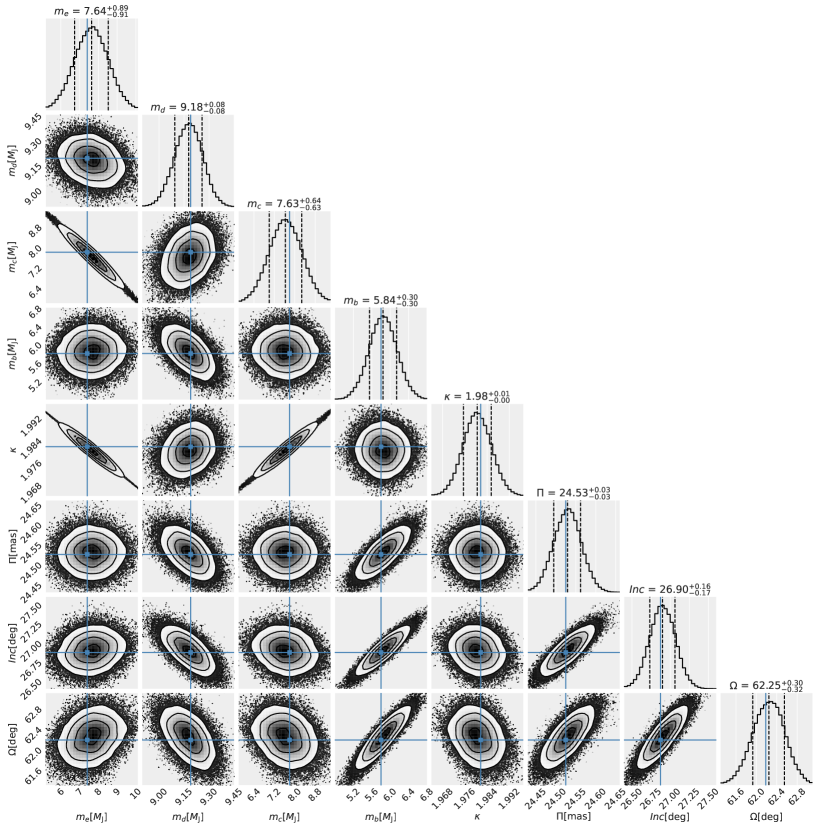
In the first step, we verified whether or not the resonant model in GM2020 based on measurements in Konopacky et al. (2016) fits the recent measurements listed in Tables 2, 3, and 5. We found that this model visually and significantly deviates from the updated data set, especially for planet HR 8799b. Therefore, we refined the PO model using the same parametrization as for the merit function; see Eq. 1 in GM2020. In the formulation presented by these latter authors, the primary parameters of the astrometric model consist of all planet masses $m_{i}$, $i=1,\ldots,4$, the osculating period ratio $\kappa$ for the two innermost planets —which selects the particular four-body Laplace resonance chain—, as well as the reference epoch $\tau$, three Euler angles $(I,\omega_{\rm rot},\Omega)$ rotating the coplanar resonant configuration to the sky (observer) plane, and the system parallax $\Pi$. This means 11 free parameters. We note that all remaining orbital parameters are constrained through the $N$-body dynamics confined to the manifold of strictly periodic solutions.

We performed the MCMC sampling from the posterior defined with the merit function in Eq. 1. This merit function is based on a numerical procedure for computing periodic solutions in a co-planar $N$-planet system, as described in GM2020 and implemented by Cezary Migaszewski (private communication). To conduct the MCMC sampling, we used the affine sampler in emcee package (Foreman-Mackey et al. 2013). We initiated 1536 walkers in a small hyper-ball in the parameter space around the initial condition in Table 6 determined with a search with the Powell non-gradient minimization algorithm. Since the auto-correlation time appears relatively short, of $\sim 100$ iterations only, we ended up with $1000$ iterations that make it possible to derive the posterior distribution, given the large number of walkers.

The derived posterior is illustrated in 2-dim projections and 1-dim histograms of the MCMC samples for the primary parameters (Fig. 1). This experiment reveals significant correlations between different parameters already reported in GM2020 that still cannot be reduced with the new data. Besides a strong $m_{\mbox{\scriptsize e}}-m_{\mbox{\scriptsize c}}$ anti-correlation, there is also $m_{\mbox{\scriptsize e}}-\kappa$ correlation and $m_{\mbox{\scriptsize d}}-\kappa$ anti-correlation. The remaining two masses are free from significant mutual correlations, however, the mass of HR 8799b appears strongly correlated with geometric parameters of the system, i.e., the Euler angles and the parallax. These parameters show mutually weaker but still significant correlations.

Parameters of the best-fitting solutions with their formal uncertainties and particular solutions from the posterior that may be useful for future numerical studies are collected in Table 6, referred to as Model IV_PO for the two stellar masses of $m_{\star}=1.52{M}_{\odot}$ and $m_{\star}=1.47{M}_{\odot}$, respectively.

For a stellar mass of $m_{\star}=1.47{M}_{\odot}$, the HR 8799d mass seems to be constrained to $\simeq 9.2\,$$M_{\mathrm{Jup}}$ within a relatively very small uncertainty of $\simeq 0.1\,$$M_{\mathrm{Jup}}$. This mass estimate is slightly larger than that found by GM2020. The mass of the outermost planet HR 8799b may be determined as $\simeq 5.8$$M_{\mathrm{Jup}}$ which is similar to $\simeq 5.5\,$$M_{\mathrm{Jup}}$ found by these latter authors, yet with also smaller uncertainty of $\simeq 0.3\,$$M_{\mathrm{Jup}}$. Moreover, for the larger stellar mass of $1.52{M}_{\odot}$, we derived slightly larger masses of HR 8799d $\simeq 9.6\pm 0.1$$M_{\mathrm{Jup}}$ and HR 8799b $\simeq 6.0\pm 0.4$$M_{\mathrm{Jup}}$.

The astrometric model for the updated data window yields $\Pi\simeq 24.26\pm 0.05$ mas, which is consistent with the earlier estimate by GM2020. The parallax estimate of $\Pi\simeq 24.53\pm 0.04$ mas derived for $1.47{M}_{\odot}$ overlaps to $1\sigma$ with $\Pi\simeq 24.460\pm 0.045$ mas in GAIA eDR3/DR3. Moreover, as noted above, when applying the parallax correction of the Lindegren et al. (2021) eDR3 catalog, Kervella et al. (2022) obtained $\Pi=24.50\pm 0.05$ mas which is even closer to the value derived from the PO model. This relation confirms the predicted strong stellar mass–parallax correlation and indirectly favors $m_{\star}=1.47\,{M}_{\odot}$. The dynamical parallax determinations appear to be very accurate and meaningful, overlapping closely with the independent geometric GAIA measurements.

Figure 1: MCMC posterior for the best-fitting, strictly resonant model derived for $m_{\star}=1.47\,$$M_{\mathrm{Jup}}$. Parameters included in the diagram are for the planet masses and orbital period ratio $\kappa=P_{\mbox{\scriptsize d}}/P_{\mbox{\scriptsize e}}=\kappa$, and parallax $\Pi$, inclination $I,$ and the nodal angle $\Omega$ (the orbital scale $\rho$, PO epoch shift $t_{0}$ and the common rotation angle $\omega_{\mbox{\scriptsize rot}}$ in the orbital planet are skipped). The crossed lines mark the best-fitting PO solution in terms of the smallest $\chi^{2}$ that was used as a starting point to initiate the emcee walkers; see Tables 6 and 7 (Model 1) for parameters of this solution. Uncertainties for the parameters are determined as the 16th and 86th percentile of the samples around the median values.

Regarding the HR 8799e–HR 8799d mass anti-correlation, we conducted additional MCMC sampling for the primary parameters in thePO model for fake data series. We prepared two or three synthetic observations per year, extending the real observations window by $\simeq 20$ years around the best-fitting periodic model with deviations and uncertainties of $\sim 1$ mas. It appears that all correlations except those between the masses and $\kappa$ would be almost eliminated. A probable cause of that effect may be the almost perfectly aligned gravitational tugs of these planets in the present particular time window of the observations. If the PO model is correct, then likely only highly precise data similar to the most accurate GRAVITY measurement in Gravity Collaboration et al. (2019) could break this degeneracy. This was indicated by GM2020. We note that the GRAVITY measurement is depicted with a star in all figures illustrating orbital solutions.

4.4 Near 8:4:2:1 MMR model

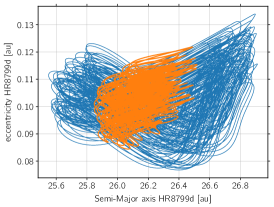
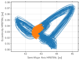
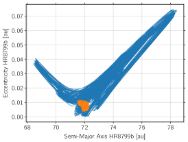
To characterize the system near the 2:1 MMR chain, we rely on the notion of the proper mean motions as the fundamental frequencies $f_{i}$ in the framework of conservative $N$-body dynamics. We resolve these frequencies with the refined Fourier frequency analysis (e.g., Laskar 1993; Nesvorny & Ferraz-Mello 1997, Numerical Analysis of Fundamental Frequencies, NAFF). To perform the NAFF, we consider the time series

$${\cal S}_{\lambda,i}=\{\,a_{i}(t_{j})\,\exp\mbox{ i}\lambda_{i}(t_{j})\,\},\quad{\cal S}_{{\cal M},i}=\{\,a_{i}(t_{j})\,\exp\mbox{ i}{\cal M}_{i}(t_{j})\,\},$$

where $j=0,1,\ldots$, $t_{j}=j\Delta t$, and $a_{i}(t)$, $\lambda_{i}(t)$ and ${\cal M}_{i}$ are the canonical osculating semi-major axis, the mean longitude, and the mean anomaly for planet $i$, $i=1,2,3,4$, respectively, and $\Delta{}t$ is the sampling interval (i is the imaginary unit). These canonical elements inferred in the Jacobi or Poincaré reference frame make it possible to account for mutual interactions between the planets to the first order in the masses.

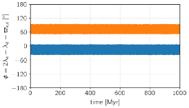
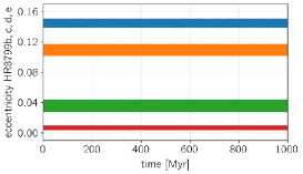
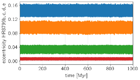
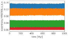
We note that the canonical orbital elements evolve differently from the common astrocentric elements. This is illustrated in Fig. 2. Subsequent panels are for the semi-major axis and eccentricity of HR 8799d,c,b, respectively, computed for the interval of a few tens of outermost orbits, and marked with different colors. It turns out that these elements span much wider ranges in the common astrocentric Keplerian frame. This effect is particularly noticeable for the two outermost planets. A small change in the $N$-body initial condition may result in substantial displacement of the orbit in the Keplerian $(a,e)$–plane. Therefore, the geometric elements should be understood as a formal representation of the Cartesian $N$-body initial conditions, and the canonical elements are more suitable for the qualitative characterization of the orbits.

Figure 2: Temporal evolution of the osculating orbital elements in the astrocentric (blue curves) and Jacobian (yellow curves) frames, respectively, for the same $N$-body initial condition implying a stable, near 8:4:2:1 MMR system. We note that the elements overlap for the first planet according to the construction of the Jacobian reference frame.

Considering a particular four-body MMR chain that can explain astrometric observations of the HR 8799 system, the zeroth-order mean-motion resonance implies one of the possible linear combinations of the fundamental frequencies (the proper mean-motions),

$$\Delta f(\@vec{k})\equiv\sum_{i=1}^{N}k_{i}f_{i},$$ (2)

where $\@vec{k}\equiv[k_{1},\ldots,k_{N}]$ is a vector of non-zero integers, and $\sum_{i=1}^{N}|k_{i}|\neq 0$, which yields small $|\Delta f|$. Simultaneously, we may determine the critical angle corresponding to $\@vec{\eta}=\mbox{arg}\min|\Delta f(\@vec{n})|$:

$$\theta_{\@vec{\eta}}(t)\equiv\sum_{i=1}^{N}\eta_{i}\lambda_{i},$$ (3)

if $\Delta{}f(\@vec{k})$ accounts only for the proper mean motions according to the d’Alembert rule. The resonant configuration may therefore be called the generalized Laplace resonance (Papaloizou 2015). This type of MMR, which possibly drives the orbital evolution of HR 8799, is characterized with the proper mean motions fulfilling the following relation (e.g., GM2020):

$$\Delta f(\@vec{k})=n_{1}-2n_{2}+n_{3}-2n_{4}.$$ (4)

Similarly to the classic Laplace resonance in the Galilean moons system, we consider the generalized MMR as a chain of two-body MMRs,

$$2n_{i+1}-n_{i}+g_{j}\simeq 2n_{i+1}-n_{i}\simeq 0,\qquad i=1,2,3,\quad j=i,i+1,$$

for subsequent pairs of planets. Here, $g_{j}$ are for the proper frequencies (mode) associated with the pericenter rotation. In the exact resonance, which we consider as the PO in the reference frame rotating with a selected planet (Hadjidemetriou 1977), the apsidal lines of all planets rotate synchronously, with the same angular velocity relative to the inertial frame. The condition in Eq. 4 for the exact resonance (periodic motion in the rotating frame) may be expressed through the proper mean motions of the planets (e.g., Delisle 2017):

$$\Delta n\equiv\sum_{i=1}^{3}\left(\frac{n_{i}}{n_{i+1}}-2\right)=0,$$ (5)

given the proper mean-motions resolved from the time series $S_{{\cal M},i}$. Numerically, we find that the exact resonance yields $\Delta{}n\simeq 10^{-13}$ rad$\cdot$d^-1 and $\Delta{}f\simeq 10^{-15}$ rad$\cdot$d^-1 for $3\times 8192$ samples of $\Delta{}t=2048$ days.

We used the resonance constraint in Eq. 5 as one of the priors for the MCMC sampling of the posterior defined through the maximum likelihood function in Eq. 1. This indirect frequency prior is Gaussian with a small variance $\sigma_{\Delta n}$ to be determined later.

We determined the frequency variance $\sigma_{\Delta n}$ based on extensive numerical experiments that relied on calibrating the $\Delta n$ range with the Lagrange (geometric) stability interval, which should not be shorter than the stellar age of $40$–$50$ Myr, as predicted in the most recent work (Brandt et al. 2021). These authors also rule out ages for HR 8799 of greater than $\approx 300$ Myr. The proper choice of the $\Delta{}n$ prior is crucial to bound (resolve) a long-term stable system in a very short integration time that spans merely a few hundred of the outermost orbits, $\simeq 2\times 10^{5}$ yr, which is also the instability timescale outside the Laplace resonance. We find, as described below in Sect. 4.6, that the astrometric HR 8799 solutions are long-term stable if $|\Delta n|$ is roughly less than $10^{-5}$–$10^{-6}$ rad$\cdot$d^-1, as described above.

4.5 Astrometric fits to near-resonance configurations

To sample the posterior defined with Eq. 1, we adopted priors described in Sect. 4.2. We did not imply any other particular limits on the anticipated near-resonant $N$-body solutions, besides uniform priors for orbital parameters in sufficiently wide ranges. In this sense, the assumed prior set is minimal. Moreover, the $N$-body model is parameterized with $(m_{i},a_{i},x_{i}\equiv e_{i}\cos\varpi_{i},y_{i}\equiv e_{i}\sin\varpi_{i},{\cal M}_{i}$), $i=1,\ldots,4$, that is, mass, semi-major axis, Poincaré elements composed of eccentricity and argument of pericenter, and the mean anomaly at the osculating epoch for each orbit, as well as two angles $(I,\Omega)$ determining the orbital plane of the system, and the astrometric parallax $\Pi$. This means 23 free parameters.

It should be noted that the implicitly defined frequency prior (Eq. 5) makes it difficult to derive the posterior distribution. In many experiments performed with a different number of MCMC walkers of up to 256 and up to 256 000 iterations, we could obtain an acceptance ratio as low as 0.1. Therefore, we understand the MCMC sampling with the $\Delta{}n$ prior as dynamically constrained optimization (rejection sampling) which helps to determine parameter ranges for the best-fitting, stable solutions. Also, due to implicit frequency prior definition, which has to be calibrated consistently with the expected dynamical stability of the system, the method has a heuristic character. Nevertheless, we may gain much insight into the parameter ranges of stable near-resonance models consistent with the astrometric observations.

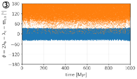
We performed many MCMC experiments varying $\sigma_{\Delta{}n}$ within the range of $10^{-7}$–$10^{-9}$ rad$\cdot$d^-1 and parameters of the emcee samplers. The example posterior for $\sigma_{\Delta{}n}=10^{-8}$ rad$\cdot$d^-1 is illustrated in Fig. 3 for parameters selected consistently with the posterior for PO shown in Fig. 1. During the sampling, we recorded all elements of the tested models, and the semi-amplitude of the critical angles of the Laplace resonance for the integration time spanning $\simeq 200$ outermost periods. Fig. 3 shows a collection of samples with $|\Delta{}n|<10^{-5}$ rad$\cdot$d^-1, and the semi-amplitude of Laplace resonance argument $|\Delta\theta|<60^{\circ}$. This choice is explained in the following Section 4.6, in which we analyze the orbital evolution of particular selected solutions.

Overall, when comparing the posterior distributions in Fig. 1 derived for the PO model, and in Fig. 4 for the quasi-periodic model, we may notice similar ranges for the parameters. A basic distinction relies on the different character of the solutions: while the PO posterior covers strictly stable, resonant solutions, the $\Delta{}n$ posterior also involves weakly chaotic solutions around the Laplace resonance center, which is selected as the starting PO model and that may explain missing mass correlations found for the PO model. While the fit quality in terms of $\ln{\cal L}$ or $\chi^{2}$ may be somewhat improved with the quasi-periodic model, the RMS of the best-fitting models remains almost the same in the two approaches. It may be concluded that the quasi-periodic model does not lead to any qualitative change in the dynamical status of the system, apart from making it possible to systematically explore long-term stable solutions, which are not necessarily regular. We discuss this further in Sect. 4.6.

Figure 3: Posterior samples for stable solutions characterized with $|\Delta{}n|<10^{-5}$ rad d^-1, and the semi-amplitude of the libration of the Laplace resonance argument $|\Delta\theta|<60^{\circ}$. The starting solution that initiated nearby MCMC walkers in the emcee samplers is the periodic configuration in Tables 6 and 7 (Model 1). Uncertainties for the parameters are determined as the 16th and 86th percentiles of the samples around the median values.

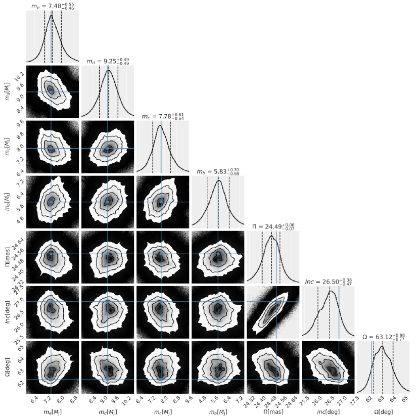
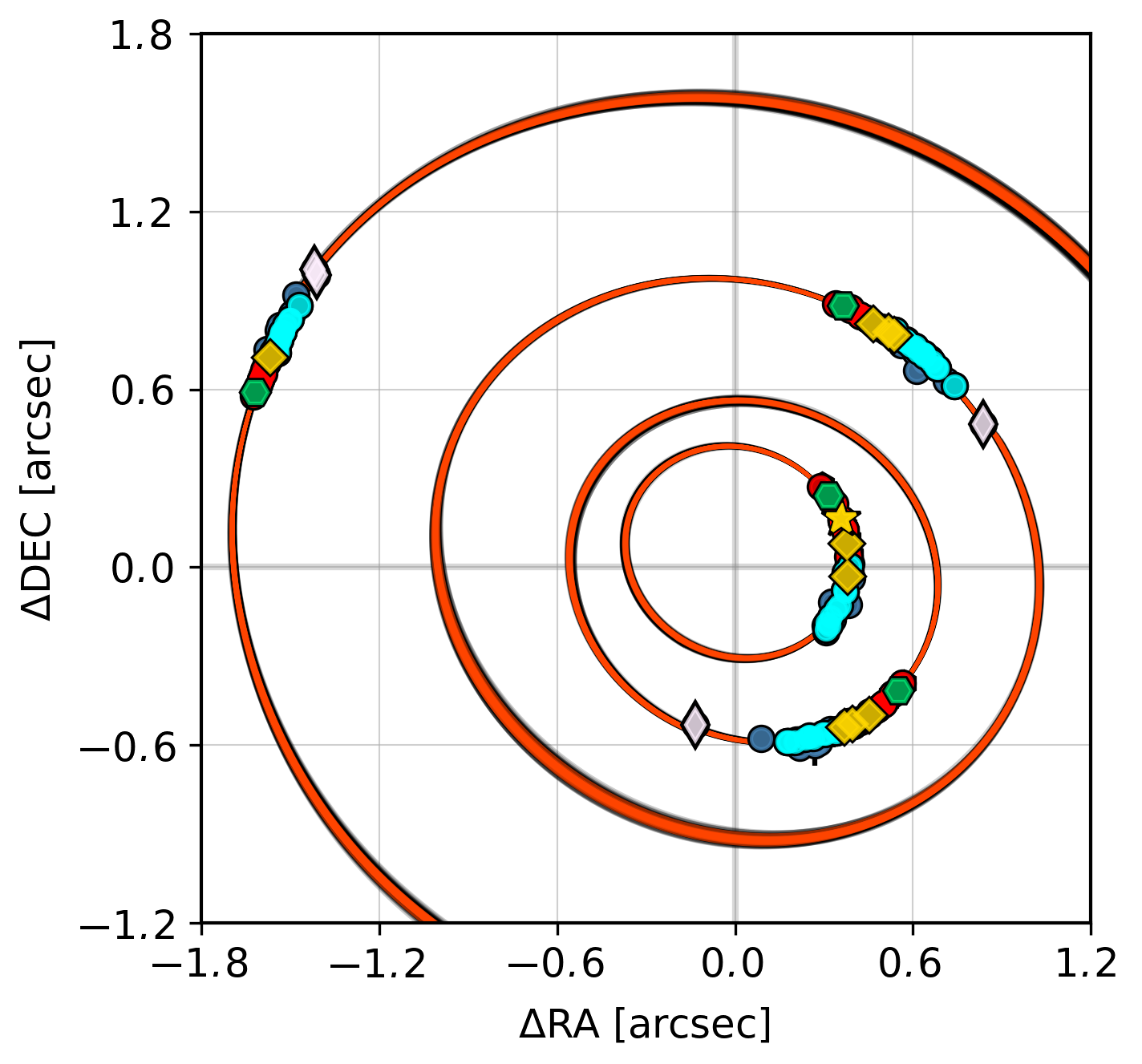
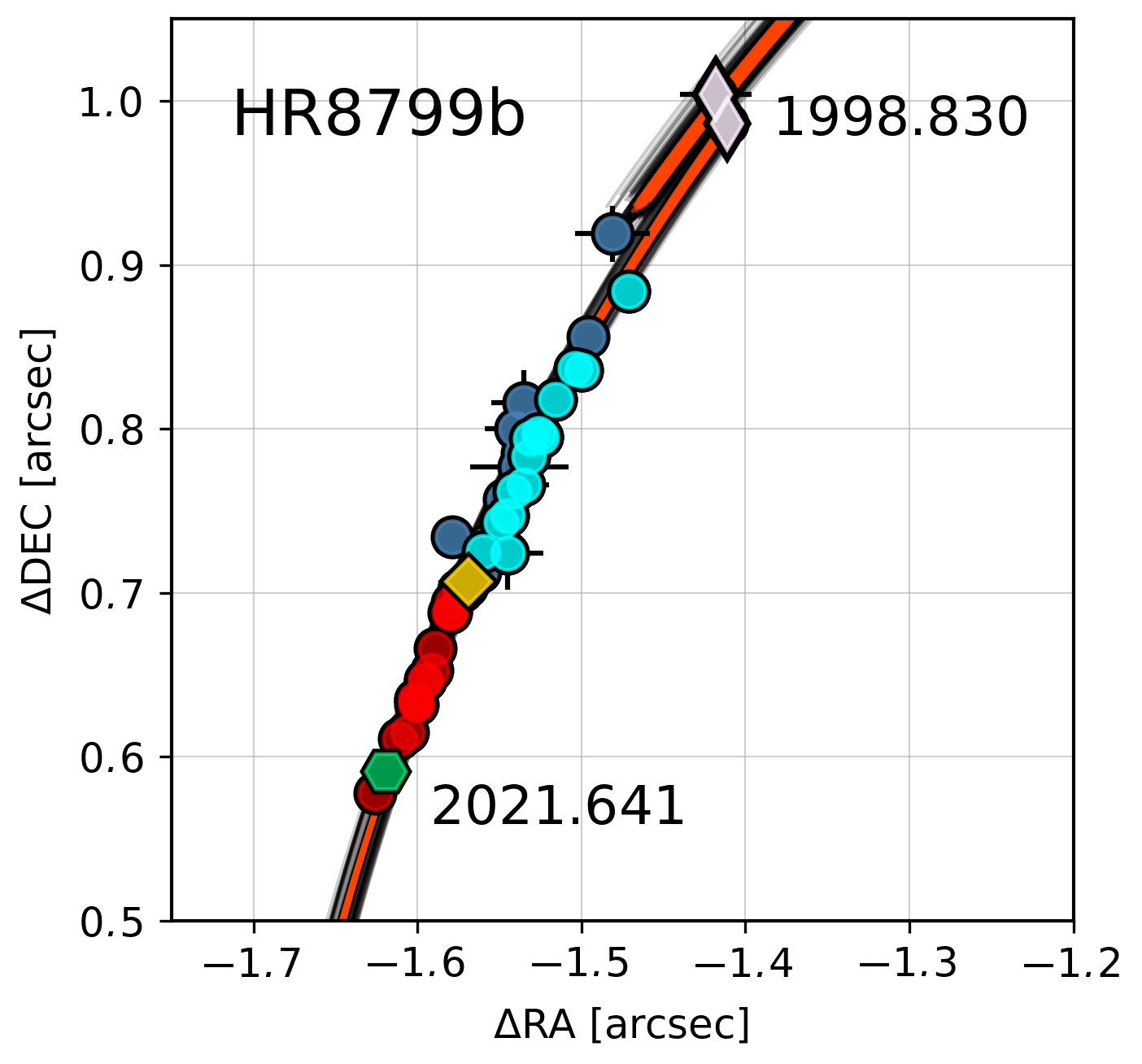
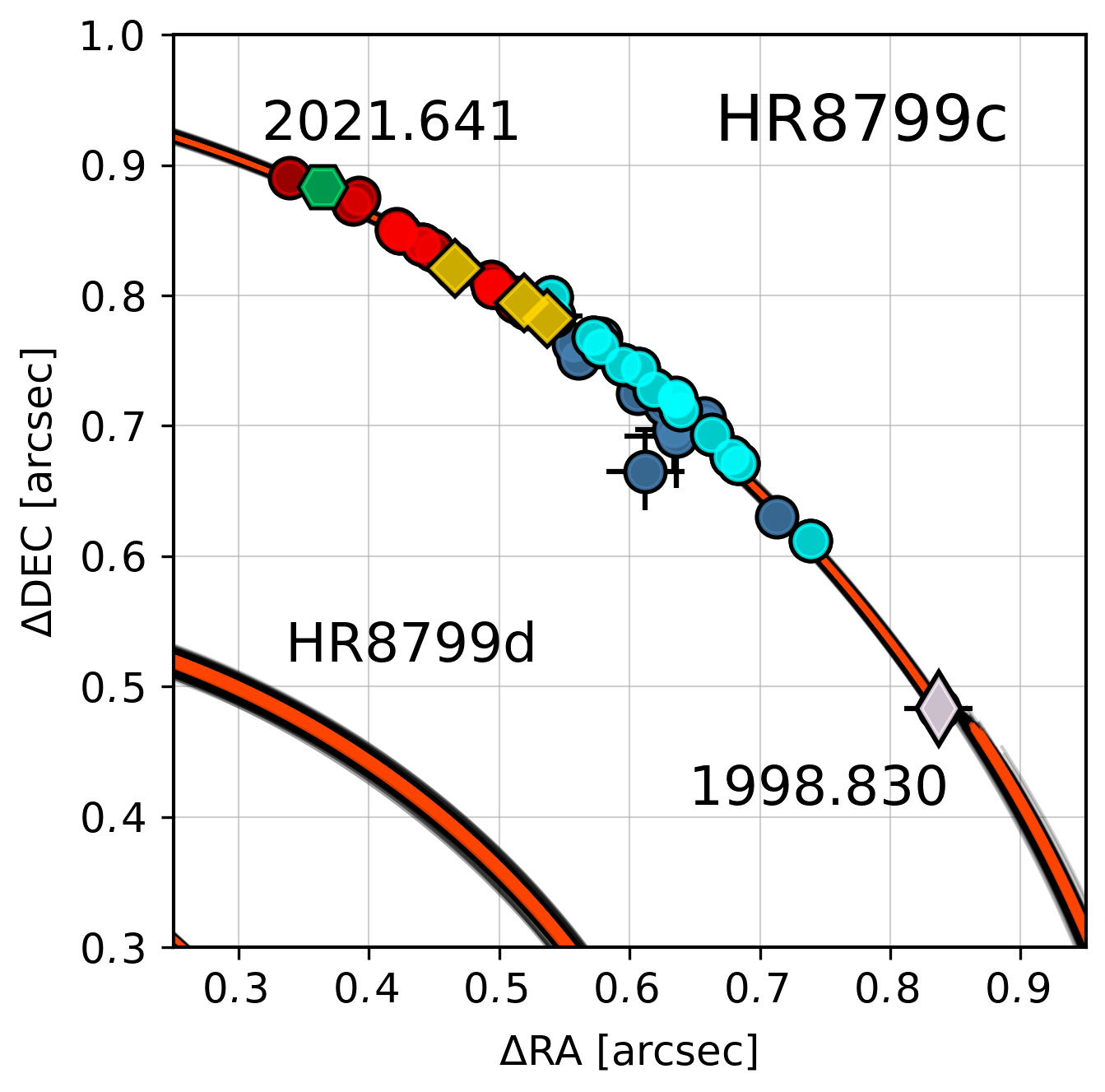
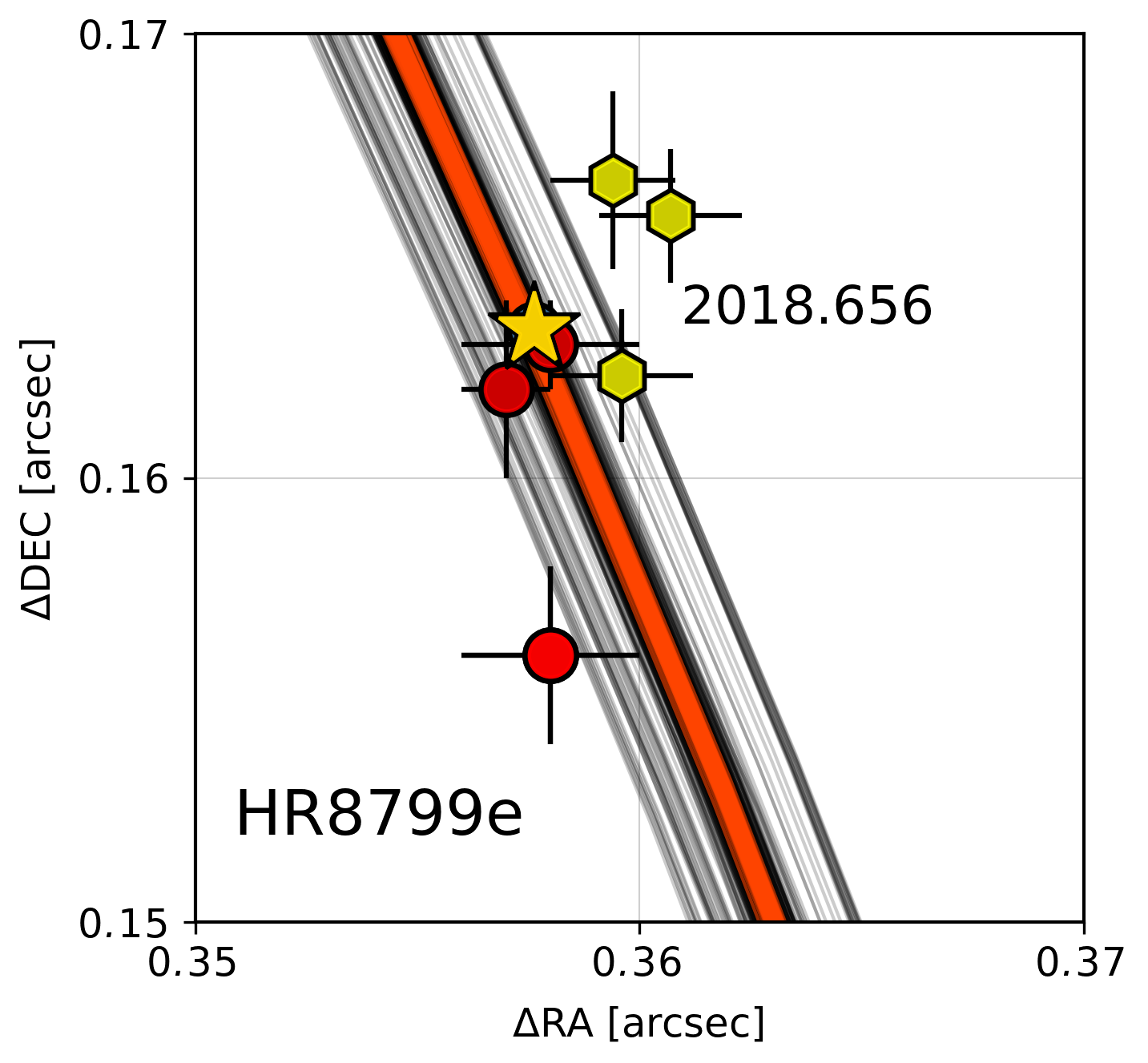
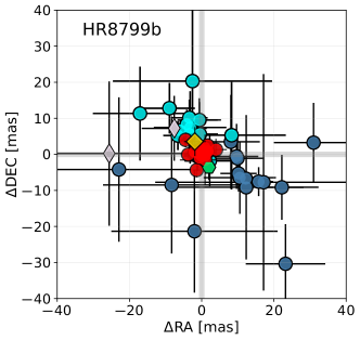
Figure 4 illustrates the best-fitting orbital solutions (red curves) over-plotted for models within $1\sigma$ (grey curves) randomly selected from the MCMC samples such that their RMS varies between $7$ and $9$ mas. The best-fitting models with RMS$\simeq 7.6$ mas are marked as red curves. All of those solutions are depicted for roughly one osculating period for each planet. Clearly, the orbits do not close for all companions. This effect is best visible for the outermost ( top-middle panel) and HR 8799d ( bottom-right panel) planet, respectively. In the latter case, the range of the orbit splitting can be compared to a relatively large uncertainty on the HST measurements; for more accurate measurements, the splitting would be even more significant. This effect illustrates strong, short-term mutual interactions. Here, we follow Goździewski & Migaszewski (2018), who indicated that Keplerian orbits are already inadequate for representing the proper astrometric solutions despite limited observational orbital arcs.

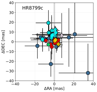
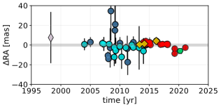
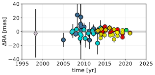
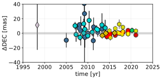
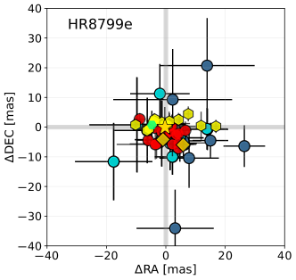
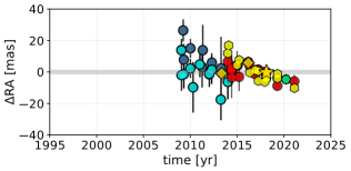
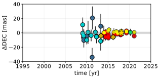
In the top-right panel Fig. 4, for HR 8799c, blue circles representing measurements in Konopacky et al. (2016) and red circles and yellow hexagons for SPHERE measurements are slightly shifted with respect to each other, and relative to the orbital model arcs. This is further visible in Figs. 5 and 6, which illustrate residuals of the best-fitting model in Table 6 in the $\Delta{}$RA–$\Delta{}$Dec-plane as well as individual $\Delta{}$RA$(t)$ and $\Delta{}$Dec$(t)$ panels. While the SPHERE data are roughly uniformly clustered around the origin $(0,0)$, the blue circles exhibit systematic patterns, especially for planets HR 8799b and HR 8799c, besides a much larger spread. This effect is curious once we recall the two data sets consisting of uniformly reduced, essentially homogeneous measurements in Konopacky et al. (2016) and this work, respectively. It is likely that the instruments and/or reduction pipelines are not fully compatible. The effect is quite subtle but still noticeable.

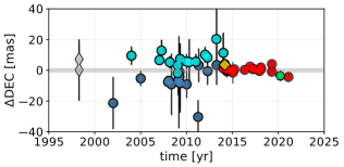
Another trend of residuals is revealed in Fig. 6 for planet HR 8799e. The SPHERE data seem to be clearly arranged along a curve in the RA coordinate, revealing a systematic deviation in time with the ephemeris. This effect is especially clear for IRDIS data and may be noted in the lower right $\Delta{}$RA-$\Delta{}$Dec panel and the $\Delta{}$RA$(t)$ panel, as the yellow hexagons spread along the $\Delta$RA=0 axis. This may indicate a systematic effect in IRDIS data reduction because it does not seem to appear for IFS data. However, the time–$\Delta$RA$(t)$ panel is suggestive of this trend for both sets of measurements. If it has no instrumental origin, then it may indicate an unmodeled component of the astrometric model, such as the presence of a yet unknown object (e.g., a distant moon) or a different curvature of the orbit due to different parameters and geometry (e.g., noncoplanarity). We note here the perfect position of the GRAVITY measurement, but this one point is insufficient to dismiss the trend.

 

Figure 4: Best-fitting solutions to the four-planet model in Table 6 for $m_{\star}=1.47$ $M_{\odot}$, illustrated on the sky plane as randomly selected MCMC samples from the $\Delta{}n$ posterior. The $y$-axis corresponds to the north ($N$), and the $x$-axis corresponds to the east ($E$) direction, respectively (we note that the numerical values of $\Delta\alpha$ are opposite in sign with respect to the formal left-hand direction of the RA $\alpha$). Red-filled circles are for the new or re-reduced IRDIS measurements in this paper, yellow hexagons are for the IFS measurements, green hexagons are for the LUCI points, light-blue filled circles are for measurements in Konopacky et al. (2016), and dark-blue circles are for data in other references collected in Tables 2, 3, and 5 and summarised in Table LABEL:t:lite. Diamonds are for the GPI data, and a star symbol is for the most accurate GRAVITY point. Red curves mark stable solutions with the lowest RMS $\simeq 7.6$–$8$ mas, randomly selected from the MCMC samples, and darker grey curves are for other orbital arcs derived for stable models up to RMS $\simeq 9$–$10$ mas. All model orbits have been derived for all measurements available to date, and cover roughly one osculating orbital period for every planet, respectively. The osculating epoch is 1998.830. We also labeled the observational epochs encompassing the orbital arcs with data. The upper left panel is for the global view of the system on the sky plane, and subsequent panels are for its close-ups and interesting regions.

 

 

Figure 5: Residuals to the selected best-fitting, near-resonant four-planet Model 2 in Table 7 for planets HR 8799b and HR 8799c; stellar mass is $m_{\star}=1.47{M}_{\odot}$. The $y$-axis corresponds to the north ($N$), and the $x$-axis corresponds to the east ($E$) direction, respectively (we note that the numerical values of $\Delta$RA are sign-opposite to regarding the formal left-hand direction of the RA axis). Red filled circles, and yellow and green hexagons are for the IRDIS, IFS, and LUCI measurements reported here, respectively, and dark-blue and light-blue (light-grey) filled circles are for measurements in previous papers and in Konopacky et al. (2016), respectively. Yellow diamonds are for GPI, the grey diamonds are for the early HST data.

 

 

Figure 6: Residuals to the best-fitting, near-resonant four-planet Model 2 in Table 7 for $m_{\star}=1.47{M}_{\odot}$, a continuation of Fig. 8 for planets HR 8799d and HR 8799e. See the caption of Fig. 5 for labels. The yellow star marks the GRAVITY measurement for HR 8799e

.

4.6 Frequency priors versus the dynamical stability

Regarding the dynamical character of solutions derived in Sect. 4.5, we analyzed representative examples of the best-fitting models marked in Fig. 4. We selected MCMC samples in Fig. 3 for $m_{\star}=1.47{M}_{\odot}$ and from other MCMC sampling for $m_{\star}=1.52{M}_{\odot}$. These initial conditions were integrated with the IAS15 integrator from the REBOUND package (Rein & Spiegel 2015) for 1 Gyr or up to disruption of the system when a collision or ejection of a planet occurs. The results are shown in a sequence of plots in Fig. 7 and Fig. 8.

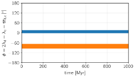
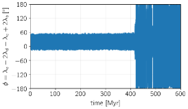
Systems illustrated in Fig. 7 are for long-term stable solutions that survived for at least 1 Gyr. The left column is for exactly resonant Model 1 and its elements displays Table 7 and also Table 6. This solution is stable forever “by design” in the framework of the $N$ body dynamics. All but one critical angle of the two-body MMRs between subsequent pairs of planets librate around centers in the $[-90^{\circ},90^{\circ}]$–range. The exceptional critical argument is for the outermost pair of planets and librates around the center at $\simeq 180^{\circ}$. As it comes to the critical argument of the Laplace resonance, it librates with a very small amplitude of just $\simeq 5^{\circ}$ around the resonance center at $\simeq 15^{\circ}$. The periodic, perfectly regular character of this solution manifests as time evolution of the eccentricities.

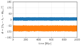
The middle column (Model 2) in Fig. 7 is for a model slightly displaced from the exact resonance, as measured by $|\Delta n|\simeq 10^{-7}$ rad$\cdot$d^-1, yet it yields slightly better fit quality. The critical arguments evolve in the same manner, as for the exact resonance, but their amplitudes and eccentricities become noticeably larger. This solution also yields a fully stable configuration of the planets. It is regular in the sense of the Lyapunov exponent, as it can be seen in Fig. 9 showing dynamical maps in terms of the MEGNO fast indicator (Cincotta et al. 2003). The mean exponential growth factor of nearby orbits (MEGNO; also known as $\langle Y\rangle$) is a numerical technique designed to efficiently characterize the stability of the $N$-body solutions in terms of the maximal Lyapunov exponent (MLE). We implemented MEGNO for the planetary problem in Goździewski et al. (2001) and in our CPU-parallelized $\mu$Farm numerical package. It is also clear that this solution lies close to the edge of the resonance island (dark blue color).

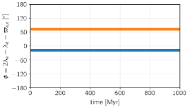
Finally, the right column (Model 3) in Fig. 7 is for a marginally stable solution, in the sense of nonzero MLE, with $|\Delta n|\simeq 10^{-5}$ rad$\cdot$d^-1. Although it survived for the 1 Gyr integration interval, one of the critical angles in the outermost 2:1 MMR rotates. This solution is peculiar in the sense that, despite rotations of one of the 2:1 MMR critical arguments, the semi-amplitudes of other critical angles are similar to those for quasi-periodic Model 2.

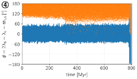
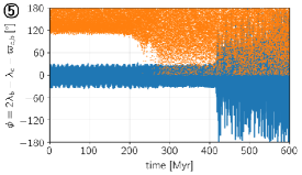
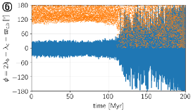
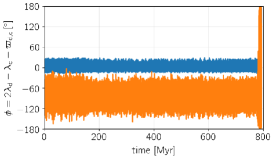
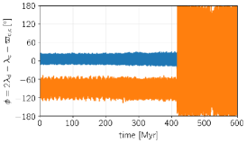
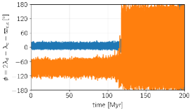
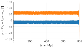
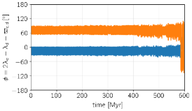
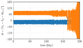
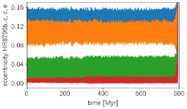
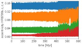
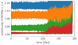
Model 3 in Fig. 7 is also remarkable when we compare it with a sequence of solutions in Fig. 8 illustrating chaotic, yet still long-term stable models characterised by $|\Delta n|\simeq 10^{-6}$ rad$\cdot$d^-1. All these models self-destruct between 800 Myr (Model 4, the left column in Fig. 8), 600 Myr (Model 5, the middle column), and just 200 Myr (Model 6, the right column). Despite this, for the initial few hundred million years, extending safely beyond most approximations of the stellar age, which range between 30–160 Myr (Baines et al. 2012; Sepulveda & Bowler 2022), the systems are bounded and locked in the resonance. Simultaneously, Models 3 and 4 yield masses of the inner planet in the $\simeq 10\,$$M_{\mathrm{Jup}}$ range, and Model 4 is especially interesting given its low $\chi^{2}$ compared to the initial starting PO configuration. These models yield a declining mass hierarchy that resembles that of the outer Solar System, and a mass of HR 8799e is consistent with the dynamical estimate in Brandt et al. (2021).

These examples are to justify that the system may be dynamically long-term stable in the planet mass range of $\simeq 10\,$$M_{\mathrm{Jup}}$, even if detuned from the exact resonance and mildly chaotic. In all unstable cases, one of the critical arguments of the 2:1 MMR of the two outermost planets progressively increases its libration amplitude and eventually begins to rotate. In this sense, the outermost pair HR 8799b–c is the weakest link in the resonance chain, provoking instability of the whole system displaced from the resonance. The time for the onset of instability can be relatively very long, as shown by the evolution of Models 4 and 5. In any case, the libration amplitudes of the critical angles seem to be a weak indicator of instability, because there is no clear relationship between these amplitudes and the time of instability. Also, Model 5 illustrates the difficulty in predicting the system behavior based on the variation of critical angles, especially if the system stability is tested for a limited period of time. The apparently regular, quasi-periodic, and bounded evolution of the critical angles for $\simeq\leavevmode\nobreak\ 200$ Myrs does not prevent the system from eventually becoming unstable after $\simeq 400$– 500 Myr. A similar effect may be observed for Model 6, although in this case, the critical argument of the Laplace resonance varies irregularly at the beginning of the integration.

It is worth noting that all of the example solutions yield astrometric fits that differ little in quality in terms of $\chi^{2}$ and RMS. The models are difficult to distinguish statistically and visually from each other. This may mean that for a coplanar, near-resonance, or resonance model we can hardly differentiate between perfectly regular and chaotic evolution of the system, as long as the instability time is sufficiently long relative to the age of the star. However, these two types of configurations occur near the exact Laplace resonance.

Figure 7: Orbital evolution of selected long-term-stable solutions with similar astrometric fit quality, but exhibiting qualitatively different stability signatures. The left column is for the exact Laplace resonance, the middle column is for a model displaced from the PO but rigorously stable, and the right column is for a $>1$ Gyr stable solution characterized by rotation of one critical angle of the 2:1 MMR in the outermost pair. The rows from the top to bottom are for all critical angles of the 2:1 MMR, the critical angle of the generalized Laplace MMR, and eccentricities for subsequent pairs of planets. See Table 7 for the initial conditions labeled from 1 to 3 at the top-left corner of each column.

Figure 8: Orbital evolution of selected long-term-stable chaotic solutions with similar astrometric fit quality. The rows from the top to bottom are for all critical angles of the 2:1 MMR, the critical angle of the generalized Laplace MMR, and eccentricities for subsequent pairs of planets. See Table 7 for the initial conditions labeled from 5 to 8 at the top of each column.

     

Figure 9: Dynamical maps in the Keplerian, osculating astrocentric semi-major-axis–eccentricity plane for the quasi-periodic, near-resonant configuration described by Model 2. All masses and elements but the map coordinates are fixed at their best-fitting values in Table 7. The osculating epoch is 1998.830. Stable solutions are determined with $|\langle Y\rangle-2|\simeq 0$ and marked with blue color.

4.7 Resonant structure of the inner debris disk

Based on the updated orbital solutions in Table 6, we revised and extended simulations of the dynamical structure of the inner debris disk in Goździewski & Migaszewski (2018). These experiments rely on the concept of the so-called $\langle Y\rangle$-model. We assume that the planets form a system of primaries in safely stable orbits robust to small perturbations. We then inject bodies with masses significantly smaller than those of the primaries and on orbits with different semi-major axes and eccentricities spanning the interesting region, and randomly selected orbital angles. Next, we integrate the synthetic configuration and determine its stability with the MEGNO ($\langle Y\rangle$) fast indicator. Calibration experiments spanning orbital evolution of debris disks in HR 8799 for up to $70$ Myr are described in detail in Goździewski & Migaszewski (2018). A comparison of the results of direct numerical integrations with the outcomes of the $\langle Y\rangle$-model confirms that these two approaches are consistent with one another, yet the $\langle Y\rangle$-based method is much more CPU efficient and therefore makes it possible to obtain a clear representation of the structure of stable solutions. This algorithm is especially effective for strongly interacting systems. Also, these simulations revealed that the close proximity of the four primaries to the exact Laplace resonance makes the system stability robust even to apparently significant perturbations caused by probe masses as large as $\simeq 2$$M_{\mathrm{Jup}}$.

We considered two types of probe objects: Ceres-like asteroids with a mass of $10^{-6}$$M_{\mathrm{Jup}}$ and Jupiter-like planets with a mass of $1$$M_{\mathrm{Jup}}$. To calculate the $\langle Y\rangle$ values for the synthetic systems, we integrated the $N$-body equations of motion and their variational equations with the Gragg-Bulirsch-Stoer integrator (Hairer et al. 2000) for $3$ Myr, which covers $6\times 10^{4}$ orbital periods of HR 8799e and $7\times 10^{3}$ orbital periods of HR 8799b, respectively. That integration time is consistent with the typical $10^{4}$ outermost orbits required to achieve $\langle Y\rangle$ convergence. We also note that the most significant interactions are exerted by the inner planets. We chose the integration time that is optimal from the CPU overhead point of view.

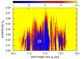
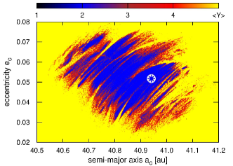
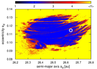
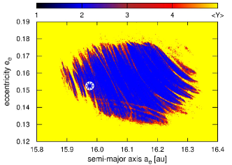
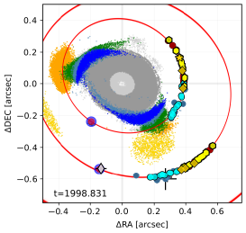
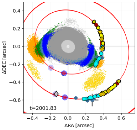
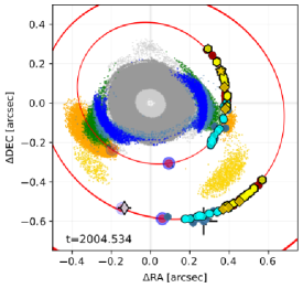
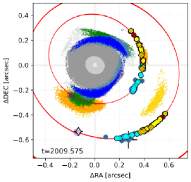
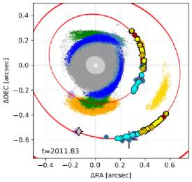
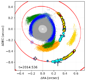
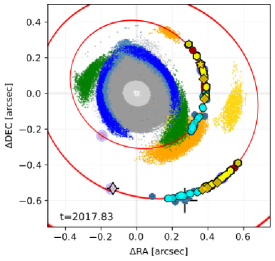
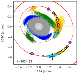
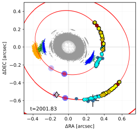
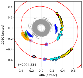
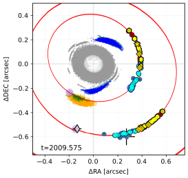
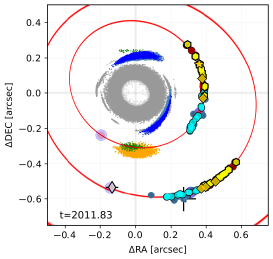
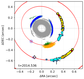
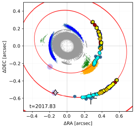
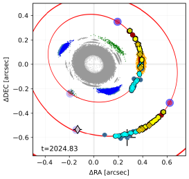
The results for the less massive Ceres-like asteroids are illustrated in Fig. 10 and Fig. 11. In this experiment, we sampled the semi-major axis $a_{0}\in[4,18]$ au and eccentricity $e_{0}\in[0,0.8]$ of these objects. We collected $3\times 10^{5}$ $N$-body initial conditions with $|\langle Y\rangle-2|<0.05$ that represent the structure of long-term-stable orbits in the inner debris disk. Subsequent panels in Figure 10 illustrate snapshots of the disk at other epochs following the first observation ($t_{0}=$1998.830) as seen on the sky plane. To obtain the snapshots, we numerically integrated the whole set of initial conditions for planets and the Ceres-like objects defined at the epoch 1998.830 up to the given final epoch $t$. For instance, $t=2009.575$ (middle-right panel) is for the first detection of the innermost planet in Marois et al. (2010).

We mark the model orbits of the two inner planets with red curves, and the astrometric measurements are over-plotted on them. Instant positions of the planets are marked with shaded large filled circles (for the first HST epoch), and large filled circles for positions of the planets at the particular epoch labeled in the lower right corner of each panel. The time range of about 30 yr is more than half the orbital period of HR 8799e and roughly one orbital period of an asteroid involved in the 2:1e MMR with this planet.

Positions of the test particles are marked with different colors depending on their dynamical status: yellow and orange dots are for objects involved in 1:1e MMR with the innermost planet HR 8799e; green dots are for the 3:2e MMR, blue dots are for the 2:1e MMR, and gray dots are for the other stable asteroids. As can be seen in Fig. 10, the outer edge of the disk is highly nonsymmetric and quickly evolves in time. Its temporal structure strongly changes even for a relatively very short interval of 25 years spanned by the astrometric observations of the system.

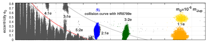
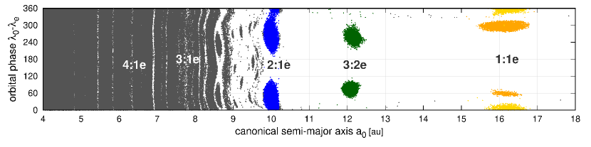
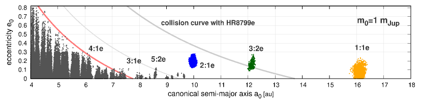
The structure of the disk has a clear resonant structure that was also noted by Goździewski & Migaszewski (2018). This is demonstrated in Fig. 11, which shows the distribution of canonical osculating elements inferred in the Jacobi reference frame, in the $(a_{0},e_{0})$-plane (top panel), and on the plane of relative orbital phases, $(a_{0},\lambda_{{\mbox{\scriptsize e}}}-\lambda_{0})$ (bottom panel). In both graphs, we mark the test particles with the same color scheme as in the previous plot, and the low-order resonances with HR 8799e are labeled. We also plot the geometrical collision curve (in gray) with planet HR 8799e constrained through the apocenter distance of the inner orbit equal to the pericenter distance of the planet, $a_{0}(1+e_{0})=a_{{\mbox{\scriptsize e}}}(1-e_{{\mbox{\scriptsize e}}})$. Also, the curve depicted in red is an image of the collision curve shifted by $\Delta{}a_{0}={4}$ au towards the star and clearly marks a boundary of stable particles.

The bottom graph shows objects involved in low-order MMRs with HR 8799e that are apparently widely spread on the sky plane, but they appear in narrow and well-localized islands on the planes of orbital elements; this is particularly clear on the $(a_{0},\lambda_{{\mbox{\scriptsize e}}}-\lambda_{0})$-plane. Both graphs mark two families of asteroids in 1:1e MMR – depicted in gold colour ($e_{0}<0.3$) and in orange ($e_{0}>0.3$). The low-eccentricity objects resemble classic Trojan asteroids in the Solar System, relative by $\pm 60^{\circ}$ to the planet. The second unusual family of highly eccentric particles in 1:1e MMR can be found on the sky plane far beyond the orbit of HR 8799e. At some epochs (e.g., 2011.83), these appear closer to the orbit of HR 8799d, which may be counter-intuitive. Given the 1:1e MMR dynamical classification, they would be expected to share the same orbit as the planet.

This simulation reveals the dynamical structure composed of long-term-stable but mutually noninteracting asteroids in the system, on the same orbit as the innermost planet, whose orbital evolution is governed by the gravitational interactions with the massive Jovian companions. Such objects should not be significantly affected by nongravitational forces, such as Poynting-Robertson drag or the Yarkovsky effect. However, such forces may be crucial for the investigation and modeling of the actual emission profile of dust produced by collisional dynamics. The results indicate that the asteroid breakup events may be frequent and violent. Given the large eccentricities and the instant mixing of different resonant fractions of these objects in the wide inner region between 4 au (and below) and 18 au, including wide Lagrange clumps of planet HR 8799e, their orbital velocity dispersion may be significant. The interplay of all these factors —and especially the clearing rate of the dust due to radiation of the young and bright host star— determines the emission profile. The present observational evidence is limited, and the position of the warm disk is estimated down to 610 au (e.g., Su et al. 2009; Matthews et al. 2014; Chen et al. 2014), which coincides with the 2:1e MMR (Fig.11); see also Sect 5. Given the topic is complex and somewhat out of the scope of the present work, we postpone in-depth analysis of the dynamical structure of the warm dust disk to a future paper.

4.8 Putative fifth Jupiter-like planet

We performed a very similar experiment for test particles of mass $1\,$$M_{\mathrm{Jup}}$, a hypothetical planet below the current detection level that may exist in the inner part of the HR 8799 system. The results are illustrated in Fig. 12 in a similar way to in Figs. 10–11. We collected $10^{5}$ stable solutions. Again, the positions of the hypothetical planet are marked at characteristic epochs; for example, near the first epoch of the HST detection, up to the last epoch of measurements in this work, and one epoch ahead of that time. Compared to the previous case, the distribution of stable objects on the plane of the sky is much narrower and more restricted. As in the case of low-mass asteroids, the positions of the putative planets can be seen to change rapidly relative to the background model orbits and astrometric measurements.

We note that the stability limit (red curve) in the bottom plot for the $(a_{0},e_{0})$- plane is offset by $\Delta{}a_{0}=6$ au with respect to the collision curve with planet HR 8799e shown in gray. In addition to the clear dependence of the structure of stable solutions on the probe mass, this simulation indicates that the hypothetical planet may be located only on very narrow islands in the orbital parameter space, limited to low-order resonances with the innermost planet. The temporal evolution of these islands in the sky can be useful for analyzing AO images and provides clues as to where an additional, Jovian planet might be expected. If such objects exist beyond $\simeq 7$ au, they should be involved in a 2:1e, 3:1e, or 5:2e MMR with the inner planet, respectively. These low-order resonances may be preferred if the system has undergone a migration in the past. We discuss this further in Sect. 5.

Attempts to find the hypothetical innermost fifth planet have so far been unsuccessful. Very recently, Wahhaj et al. (2021), using SPHERE measurements also reported here, did not detect planet HR 8799f at the most plausible locations, namely 7.5 and 9.7 au, down to mass limits of 3.6 and $2.8\,$$M_{\mathrm{Jup}}$, respectively. Neither did these authors detect any new candidate companions at the smallest observable separation, of namely 0.1$"$ or $\simeq 4.1$ au, overlapping with the semi-major axes range in Fig. 10–12. Wahhaj et al. (2021) conclude that the planet may still exist with a mass of $2$-$3.6\,$$M_{\mathrm{Jup}}$ at 7.5 au (3:1e MMR) or $1.5$-$2.8\,$$M_{\mathrm{Jup}}$ at 10 au, which is in the region we closely investigated in this section. The contrast curve in the interesting zone between roughly 7 and 16 au lies above roughly three Jupiter masses, as also concluded here; see Fig. 15 and discussion in Sect. 6. Therefore, we believe that steadily improved imaging techniques, gaining better contrast and lower detection limits, combined with dynamical simulations similar to those conducted in this section may eventually reveal the fifth planet. However, if a relatively massive planet of mass $\simeq 1\,$$M_{\mathrm{Jup}}$ exists in the inner part of the system, the outer edge of the debris disk carved out by this planet would have a much smaller radius than predicted at $\simeq 10$ au under the current observational configuration of four planets (Fig. 11), and related to the above-mentioned detections of warm dust at $6$–$10$ au (e.g., Su et al. 2009; Hughes et al. 2011; Matthews et al. 2014; Chen et al. 2014). We defer the analysis of this situation to a future work as well, because of its complexity arising from different MMR scenarios.

Figure 10: Evolution of the inner debris disk as seen on the plane of the sky. The subsequent panels show the instantaneous positions of two inner planets and small asteroids in stable orbits (small colored dots) with a mass of $10^{-6}\,$$M_{\mathrm{Jup}}$ at the epoch labeled in the lower-left corner of each graph. We collected $3.3\times 10^{5}$ particles. Their distribution in the $(a_{0},e_{0})$-plane of osculating, canonical elements at the initial epoch 1998.830 is shown in Fig. 11. The largest filled circles correspond to the positions of the planets HR 8799e and HR 8799d at the snapshot epoch (large filled circles) and the initial osculating epoch (shaded filled circles), respectively. The asteroid colors are for the lowest order MMR types, as indicated in the bottom two plots, or those belonging to the innermost quasi-homogeneous disk (gray points). The 2024.83 epoch covers roughly one orbital period in a 2:1e MMR resonance (dark blue circles) with the innermost planet.

Figure 11: Structure of the inner debris disk composed of $3\times 10^{5}$ Ceres-like asteroids of mass $10^{-6}\,$$M_{\mathrm{Jup}}$ on stable orbits, seen in the $(a_{0},e_{0})$-plane of Jacobian (canonical) osculating elements at the initial 1998.830 epoch. The colors of the asteroids indicate the lowest order MMR in which they are involved with HR 8799e, as indicated in the diagrams, or belong to the innermost, quasi-homogeneous disk (gray points) according to Fig. 10. The light gray curve indicates the collision of the orbits with HR 8799e and the red curve is an image of the collision curve shifted by $\Delta{}a_{0}\simeq{4}$ au toward the star. We note that loose points above the collision curve in the top panel represent immediately scattered asteroids on regular but hyperbolic (open) orbits.

Figure 12: Possible instant positions (small gray and colored dots) of a hypothetical and still undetected planet of mass $1\,$$M_{\mathrm{Jup}}$ on the sky plane, at the epoch labeled in the lower-left corner of each graph. We collected $10^{5}$ initial conditions. The bottom plot shows their distribution in the $(a_{0},e_{0})$–plane of canonical osculating elements at the initial epoch of 1998.830, similarly to Fig. 11. As in Fig. 10, the largest filled circles correspond to the positions of the planets HR 8799e and HR 8799d at the snapshot epoch (large filled circles) and the initial osculating epoch (shaded filled circles), respectively. Colors mark the lowest order MMR types, as labeled in the bottom plot. The light-gray curve marks the collision zone with HR 8799e, the thinner curve marks the stability zone for $m_{0}=10^{-6}\,$$M_{\mathrm{Jup}}$ (see Fig. 10), and the red curve is the image of the geometric collision curve shifted by $\Delta{}a_{0}\simeq{6}$ au toward the star.

Table 6: Osculating, heliocentric elements of the best-fitting solutions at the epoch of 1998.830. The stellar mass is $m_{\star}=1.52\,{M}_{\odot}$ or $m_{\star}=1.47\,{M}_{\odot}$. Uncertainties for parameters in models IV_PO and IV_Δn are determined as the 16th and 86th percentiles of the samples. Parameter values with 8–9 significant digits are provided in order to reproduce the results of particular integrations. Parameter $\nu=N_{\rm obs}-\dim{\@vec{p}}$ is for the degrees of freedom, where $N_{\rm obs}$ denotes the number of $(\alpha,\delta)$ measurements, and $\dim{\@vec{p}}$ is the number of free parameters.

Model IVPO:  $m_{\star}=1.52\,{M}_{\odot}$,  $\Pi=24.2585686$ mas $(24.26\pm 0.05)$ mas,  $\chi^{2}_{\nu}=4.32$, $\nu=441$, $\dim{\@vec{p}}=11$
	$m\,[{M}_{{\mbox{\scriptsize Jup}}}]$	$a\,$[au]	$e$	$I\,$[deg]	$\Omega\,$[deg]	$\varpi\,$[deg]	$\mathcal{M}\,$[deg]
HR 8799e	$8.1\pm 0.7$	$16.28\pm 0.03$	$0.147\pm 0.001$			$110.8\pm 0.5$	$336.8\pm 0.5$
	8.24465258	16.2817072	0.147508399			110.765660	336.793683
HR 8799d	$9.5\pm 0.1$	$26.78\pm 0.08$	$0.115\pm 0.001$			$29.4\pm 0.9$	$59.8\pm 0.8$
	9.48438158	26.7888442	0.01154150			29.4676779	59.6448288
HR 8799c	$7.7\pm 0.5$	$41.40\pm 0.10$	$0.055\pm 0.002$	$26.9\pm 0.2$	$62.2\pm 0.4$	$92.1\pm 0.5$	$145.6\pm 0.8$
	7.64047381	41.3945527	0.05485344	26.8923597	62.2416412	92.1126122	145.7203489
HR 8799b	$6.0\pm 0.4$	$71.95\pm 0.13$	$0.017\pm 0.001$			$44.4\pm 3.0$	$309.2\pm 2.6$
	6.01476193	71.9477733	0.017597398			44.6384383	309.291519
Model IVPO:  $m_{\star}=1.47\,{M}_{\odot}$,  $\Pi=24.5256617$ mas $(24.53\pm 0.04)$ mas,  $\chi^{2}_{\nu}=4.32$, $\nu=441$, $\dim{\@vec{p}}=11$
	$m\,[{M}_{{\mbox{\scriptsize Jup}}}]$	$a\,$[au]	$e$	$I\,$[deg]	$\Omega\,$[deg]	$\varpi\,$[deg]	$\mathcal{M}\,$[deg]
HR 8799e	$7.6\pm 0.9$	$16.10\pm 0.03$	$0.148\pm 0.001$			$110.8\pm 0.5$	$336.8\pm 0.3$
	7.4060918	16.1038912	0.147675953			110.816707	336.828050
HR 8799d	$9.2\pm 0.1$	$26.46\pm 0.09$	$0.115\pm 0.002$			$29.1\pm 1.0$	$60.0\pm 1.0$
	9.18999484	26.45172667	0.114600334			29.0594738	60.1752106
HR 8799c	$7.7\pm 0.7$	$40.97\pm 0.10$	$0.054\pm 0.002$	$26.9\pm 0.2$	$62.2\pm 0.4$	$92.3\pm 0.6$	$145.5\pm 0.7$
	7.79611845	40.9861801	0.05380902	26.8734271	62.1852189	92.3879462	145.5347082
HR 8799b	$5.8\pm 0.4$	$71.14\pm 0.15$	$0.017\pm 0.002$			$43.50\pm 3.0$	$310.35\pm 3.0$
	5.80235941	71.1427851	0.01667073			42.9704380	310.895065
Model IVΔn:  $m_{\star}=1.47\,{M}_{\odot}$,  $\Pi=24.5256617$ mas $(24.49\pm 0.07)$ mas,  $\chi^{2}_{\nu}=3.9$, $\nu=429$, $\dim{\@vec{p}}=23$
	$m\,[{M}_{{\mbox{\scriptsize Jup}}}]$	$a\,$[au]	$e$	$I\,$[deg]	$\Omega\,$[deg]	$\varpi\,$[deg]	$\mathcal{M}\,$[deg]
HR 8799e	$7.5\pm 0.6$	$16.00\pm 0.10$	$0.150\pm 0.004$			$108.8\pm 1.3$	$336.00\pm 1.5$
	7.40609179	16.1038912	0.147675954			110.816707	336.828050
HR 8799d	$9.3\pm 0.5$	$26.55\pm 0.12$	$0.114\pm 0.004$			$28.66\pm 1.2$	$60.0\pm 1.0$
	9.18999484	26.45172667	0.11460033			29.05947383	60.1752106
HR 8799c	$7.8\pm 0.6$	$41.00\pm 0.15$	$0.050\pm 0.003$	$26.5\pm 0.5$	$63.1\pm 0.5$	$91.8\pm 1.0$	$145.0\pm 1.0$
	7.79611845	40.9861801	0.05380902	26.8734271	62.1852189	92.3879462	145.5347082
HR 8799b	$5.8\pm 0.8$	$71.3\pm 0.2$	$0.017\pm 0.002$			$42.3\pm 1.6$	$310.8\pm 2.0$
	5.80235941	71.1427851	0.016670734			42.9704380	310.895065

Table 7: Osculating, heliocentric elements of the best-fitting solutions at the epoch of $1998.83$ for models illustrated in Figure 4 and in Figs. 7–8.

Model 1:  $m_{\star}=$1.47 $M_{\odot}$,  $\Pi=$ 24.525662 mas,  $\chi^{2}$=1593.22,  RMS$=$7.41 mas,  $\log|\Delta{}n[\mbox{rad}\,\mbox{d}^{-1}]|$=-12.0
	$m\,[{M}_{{\mbox{\scriptsize Jup}}}]$	$a\,$[au]	$e$	$I\,$[deg]	$\Omega\,$[deg]	$\omega\,$[deg]	$\mathcal{M}\,$[deg]
HR8799e	7.4060918	16.1038912	0.1476760	26.8734271	62.1852189	110.8167067	-23.1719500
HR8799d	9.1899948	26.4517267	0.1146003	26.8734271	62.1852189	29.0594738	60.1752106
HR8799c	7.7961185	40.9861801	0.0538090	26.8734271	62.1852189	92.3879462	145.5347082
HR8799b	5.8023594	71.1427851	0.0166707	26.8734271	62.1852189	42.9704380	-49.1049354
Model 2:  $m_{\star}=$1.47 $M_{\odot}$,  $\Pi=$ 24.451807 mas,  $\chi^{2}$=1568.19,  RMS$=$7.66 mas,  $\log|\Delta{}n[\mbox{rad}\,\mbox{d}^{-1}]|$=-6.2
	$m\,[{M}_{{\mbox{\scriptsize Jup}}}]$	$a\,$[au]	$e$	$I\,$[deg]	$\Omega\,$[deg]	$\omega\,$[deg]	$\mathcal{M}\,$[deg]
HR8799e	7.8680000	15.9753973	0.1524708	26.2394739	63.7770393	108.3445443	335.6210695
HR8799d	9.6490000	26.6396632	0.1145654	26.2394739	63.7770393	28.3126706	59.7394429
HR8799c	7.3081300	40.9406369	0.0517422	26.2394739	63.7770393	91.3551907	145.0637721
HR8799b	5.6590700	71.3289844	0.0173411	26.2394739	63.7770393	41.6627885	310.5199311
Model 3:  $m_{\star}=$1.52 $M_{\odot}$,  $\Pi=$ 24.347839 mas,  $\chi^{2}$=1624.73,  RMS$=$7.66 mas,  $\log|\Delta{}n[\mbox{rad}\,\mbox{d}^{-1}]|$=-4.5
	$m\,[{M}_{{\mbox{\scriptsize Jup}}}]$	$a\,$[au]	$e$	$I\,$[deg]	$\Omega\,$[deg]	$\omega\,$[deg]	$\mathcal{M}\,$[deg]
HR8799e	8.9817200	16.1163303	0.1548634	27.3470617	62.9005413	108.0955330	336.2997163
HR8799d	9.0680400	26.8768634	0.1068892	27.3470617	62.9005413	29.2629241	60.0277429
HR8799c	7.2212900	41.0832702	0.0627005	27.3470617	62.9005413	91.9708727	144.7587008
HR8799b	6.1950900	71.7822044	0.0192741	27.3470617	62.9005413	44.4483815	308.9107410
Model 4:  $m_{\star}=$1.52 $M_{\odot}$,  $\Pi=$ 24.305464 mas,  $\chi^{2}$=1564.70,  RMS$=$7.64 mas,  $\log|\Delta{}n[\mbox{rad}\,\mbox{d}^{-1}]|$=-6.2
	$m\,[{M}_{{\mbox{\scriptsize Jup}}}]$	$a\,$[au]	$e$	$I\,$[deg]	$\Omega\,$[deg]	$\omega\,$[deg]	$\mathcal{M}\,$[deg]
HR8799e	10.6577500	16.1274692	0.1496852	26.9747476	63.6149718	107.6133926	336.6560551
HR8799d	9.5739000	26.8852716	0.1169394	26.9747476	63.6149718	27.5720349	60.0200173
HR8799c	6.8413200	41.2618982	0.0555455	26.9747476	63.6149718	93.1349542	143.0235158
HR8799b	5.7085500	71.9446080	0.0217920	26.9747476	63.6149718	45.1149621	307.6876430
Model 5:  $m_{\star}=$1.47 $M_{\odot}$,  $\Pi=$ 24.466345 mas,  $\chi^{2}$=1591.33,  RMS$=$7.63 mas,  $\log|\Delta{}n[\mbox{rad}\,\mbox{d}^{-1}]|$=-6.9
	$m\,[{M}_{{\mbox{\scriptsize Jup}}}]$	$a\,$[au]	$e$	$I\,$[deg]	$\Omega\,$[deg]	$\omega\,$[deg]	$\mathcal{M}\,$[deg]
HR8799e	7.1130900	15.9976012	0.1545297	26.5969851	62.8989533	108.8687608	336.1919760
HR8799d	9.8864900	26.5290674	0.1122973	26.5969851	62.8989533	27.8297522	61.2151462
HR8799c	7.7520500	41.1188833	0.0497536	26.5969851	62.8989533	92.4070918	144.9763772
HR8799b	5.5380200	71.3013150	0.0172797	26.5969851	62.8989533	44.6821435	308.5634968
Model 6:  $m_{\star}=$1.47 $M_{\odot}$,  $\Pi=$ 24.539234 mas,  $\chi^{2}$=1568.59,  RMS$=$7.63 mas,  $\log|\Delta{}n[\mbox{rad}\,\mbox{d}^{-1}]|$=-6.2
	$m\,[{M}_{{\mbox{\scriptsize Jup}}}]$	$a\,$[au]	$e$	$I\,$[deg]	$\Omega\,$[deg]	$\omega\,$[deg]	$\mathcal{M}\,$[deg]
HR8799e	7.3387300	15.9246991	0.1553777	26.5990408	62.7197878	108.3820177	336.0139713
HR8799d	10.0516400	26.5092120	0.1117405	26.5990408	62.7197878	29.2671129	59.8339479
HR8799c	8.0973100	40.9565104	0.0509428	26.5990408	62.7197878	91.8212168	145.6257159
HR8799b	5.8932800	71.1073028	0.0167537	26.5990408	62.7197878	41.9648749	311.2692413

5 Possible history of the system

Convergent migration due to tidal interaction with the nesting circumstellar disk is thought to be the most reliable mechanism for producing resonance trapping in multiple-planet systems (Masset & Snellgrove 2001; Lee & Peale 2002; Moorhead & Adams 2005; Thommes 2005; Beaugé et al. 2006; Crida et al. 2008; D’Angelo & Marzari 2012). The different masses of the planets and progressive inside-out depletion of gas in the disk due to the presence of the planet itself and photo-evaporation lead to different migration speeds for the planets, which may end up in resonance. Numerical modeling by Hands et al. (2014) and Szuszkiewicz & Podlewska-Gaca (2012) shows that during inward migration, planets are often trapped in resonances like the 2:1 and 3:2 (the most frequent).

While in most resonant cases, such as Gliese 876, HD 82943, and HD 37124 (Wright et al. 2011), the planets are close to the star, in the case of HR 8799 the planets are significantly far away. This implies that the primordial disk from which they formed should have extended beyond 100 au which is compatible with the mass of the star being $\sim$1.5 $M_{\odot}$. The most robust scenario is that in which the planets were fully formed further out in the disk and then migrated inwards until they became progressively trapped in the multiple resonances. This scenario raises the question of whether these planets were formed by core accretion (Mizuno 1980; Pollack et al. 1996) or by gravitational instability (Cameron 1978; Boss 1997).

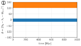
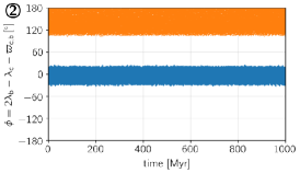
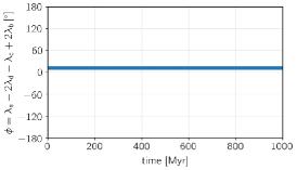
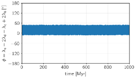
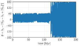
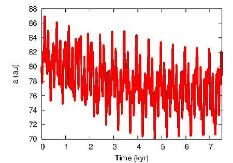
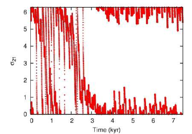
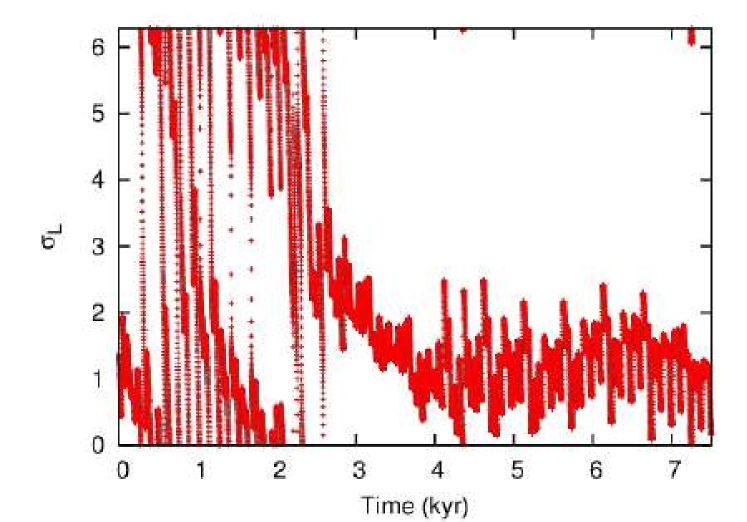
The resonance trapping in this system at that distance from the star is confirmed by hydrodynamical simulations performed with the FARGO code (Masset 2000). Fully radiative models have been adopted where the energy equation contains viscous heating and radiative cooling through the disk surface. A polar grid with $682\times 512$ elements is used to cover the disk, extending from 1 to 120 au. The initial surface gas density is given by $\Sigma=\Sigma_{0}r^{-1/2}$ with $\Sigma_{0}=50$ g$/$cm². This low density is motivated by the evolved state of the disk when the planets are fully formed. To test the sequential resonance trapping, we start the inner planets on already resonant orbits; they are not affected by the disk, and so do not migrate. The outer planet instead feels the disk perturbations and migrates inward until it is trapped in the 2:1 resonance and stops migrating. This behavior is illustrated in Fig. 13 where in the top panel the semi–major axis of the fourth planet is shown while in the middle and bottom panels the critical argument of the 2:1 resonance between the third and fourth planet and the Laplace resonance argument is illustrated.

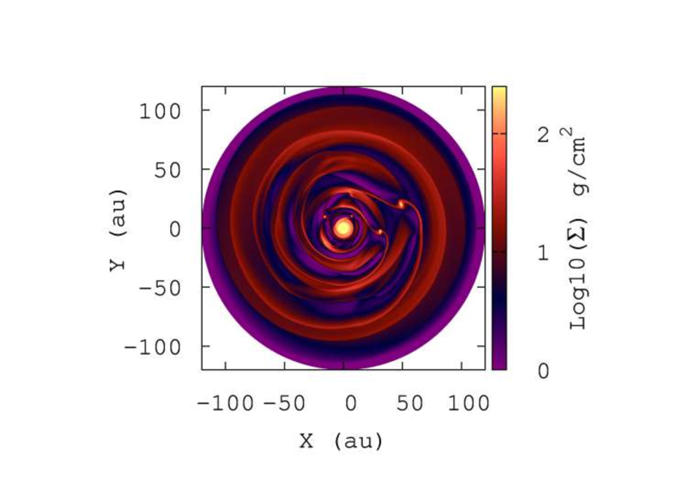
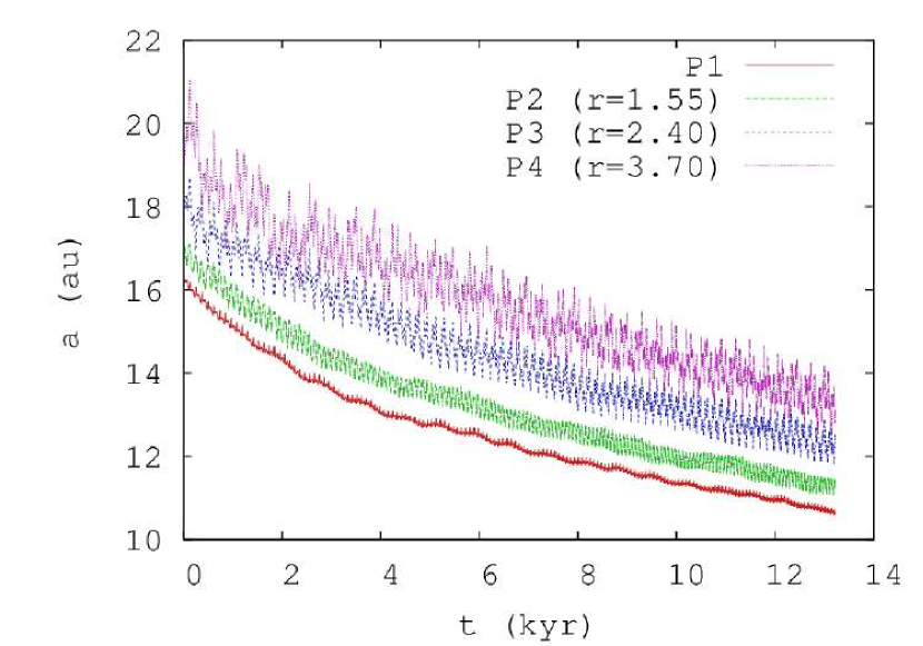
It is noteworthy that, once all the planets are trapped in resonance, they share a common gap and migrate inwards. We performed an additional simulation where all four planets are affected by the disk perturbations and can freely migrate. In this simulation, we increased $\Sigma_{0}$ to 100 g$/$cm² in order to speed up the migration. Figure 14 shows the gas density distribution after 8 Kyr from the beginning of the simulation. The planets create a common gap where some overdensities are still present in the corotation regions of each planet. The semi-major axes of the planets are illustrated in the bottom panel, rescaled to be shown in a single plot. They migrate inwards while trapped in resonance, suggesting that the present position of the planets is not necessarily the one where they became trapped in resonance. The capture in the mutual resonance may have occurred farther out, followed by an inward migration until the disk dissipates. This may push the location where the planet initially grew even farther out. It is noteworthy that the wider oscillations observed in the critical arguments of the resonances and the semi-major axis of the planets compared to a pure $N$–body problem are related to the presence of the perturbations of the disk on the planets.

Figure 13: Resonance trapping of the HR 8799 system during the migration phase. The upper panel shows the evolution of the semi-major axis of the outer planet at the moment of capture in resonance with the inner three bodies. After the resonance trapping, the semi-major axis remains constant. The middle panel shows the critical argument of the resonance between the two outer planets. After the capture in resonance, the critical argument librates. The same occurs for the Laplace critical argument shown in the bottom panel.

Figure 14: Orbital evolution of the HR 8799 system during the migration phase. The upper panel shows the gas density of the disk. The bottom panel shows the semi-major axes of the planets rescaled with constant values for ease of visualization in the same plot.

6 Planets–disk interaction

Along with the four giant planets detected so far, the architecture of HR 8799 is enriched by the presence of an extended debris disk with two components. The cold Kuiper-like component was resolved in the FIR (Matthews et al. 2014) and at millimeter wavelengths (Booth et al. 2016; Wilner et al. 2018) and was detected up to 450 au from the star, with a halo extending to thousands of astronomical units (au). The warm component was instead never fully resolved and its inferred position of $9.3$ au is given by modeling the IR excess at 155 K (Chen et al. 2014) in the SED of the star under the assumption of dust particles behaving like black bodies. The two components are separated by a huge dust-free gap that extends from 109 au (Wilner et al. 2018) to regions interior to the orbit of HR 8799e.

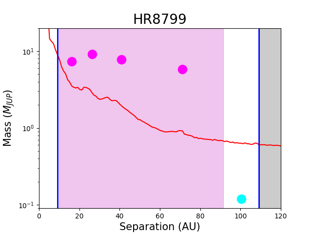
As the presence of the gap is tightly correlated with the planets in it, we can assess the planets–disk interactions and infer whether or not the planets detected are responsible for carving the entire gap or whether or not there is further dynamical space for hosting other undetected planets. For this analytical study, the only planets taken into account are the two closest to the edges of the gap, HR 8799 b and e. The orbital parameters and masses adopted are the ones listed in Tables 6 and 7 for Model 1. To calculate the extension of the region from which dust particles are scattered away from the orbit of the planet (chaotic zone), we used Eqs. 9 and 10 of Lazzoni et al. (2018) for HR 8799b and HR 8799e, respectively. As a result, we obtained that the chaotic zone of the inner planet extends down to 9.8 au, which is consistent with the direct $N$-body simulations in Sect. 4.7. Given the uncertainties on the position of the inner belt and on its width, we can safely state that HR 8799e is likely responsible for shaping the inner edge of the gap. On the other hand, the chaotic zone for HR 8799b can clear the orbit of the planet up to 91.4 au. Given the position of the outer edge of the gap at 109 au, we can try to infer the characteristics of a fifth planet able to extend the chaotic zone up to the detected position of the edge. Following a very simple approach, we can use the same analytical tools to estimate the mass and semi-major axis of a planet able to carve a gap extending from 91.4 au to 109 au, that is, the free dynamical region left beyond the orbit of HR 8799b. As a result, we obtain a $0.12$ $M_{\mathrm{Jup}}$ planet orbiting at 100 au.

Figure 15 shows a summary of the results discussed above. The four detected planets are represented as pink circles together with the extension of their chaotic zone (pink shaded area). As it emerges from the image, the inner extension of the clearing zone gets very close to the inner belt (blue vertical line) whereas it stops roughly $20$ au from the outer belt. Even a very low mass planet could carve the remaining part of the gap and, consistently with our observations, it would be too small to be detected with an instrument such as SPHERE, as proven by the detection limits (red curve; IRDIS data taken on 2017 October 12) shown in the figure. Simulations of the inner debris disk in the framework of the $N$-body resonant model of the system in Sect. 4.7 indicate possible localizations of such a planet. We want to stress that this is only a preliminary analysis of the planet–disk interaction. More detailed studies will have to consider the dynamical interaction of the fifth planet with all four of the detected ones as well as the possibility of having a larger object locked in MMR with at least one of the other known planets, as discussed in the following.

Indeed, the results of numerical $N$-body simulations in Goździewski & Migaszewski (2018) based on the $\langle Y\rangle$-model described in Sect. 4.7 partially confirm the analytical predictions and address the likely real resonant configuration of the planets. These latter authors simulated the inner edge of the outer debris disk, also accounting for the presence of a hypothetical fifth planet with a mass between $0.1$ and $1.66$ $M_{\mathrm{Jup}}$. These simulations are based on a quasi-periodic, near-resonant orbital model of the four known planets derived through migration simulations. However, given that Goździewski & Migaszewski (2018) adopted the larger mass for the star of $m_{\star}=1.52$$M_{\odot}$ and a larger parallax $\Pi=25.4$ mas, the whole system appears more compact than predicted at present — these authors found the osculating astrocentric semi-major axis of HR 8799b $\simeq 67.1$ au, compared to $\simeq 71$ au in the present models. The updated values of the parallax and the stellar mass translate to orbits expanded by a few au. According to the simulations, the inner edge of the outer disk is globally highly nonsymmetric, and planets with a mass of between $0.1$ and $1.66$ $M_{\mathrm{Jup}}$ may be present beyond the clearing zone, with semi-major axis $>90$ au. These planets could be involved in low-order resonances, such as 3:2b, 5:3b, 2:1b, or 5:2b with the outermost planet HR 8799b and in low and moderate eccentricity orbits; see Fig. 9 in Goździewski & Migaszewski (2018). The fifth planet, even if it had a small mass, would be strongly affecting the shape of the inner parts of the outer debris disk.

Figure 15: HR 8799 architecture: two belts (blue lines), four detected planets (pink circles), and a putative fifth planet (light-blue circle). The pink shaded area represents the extension of the chaotic zone whereas the gray shaded zone represents the extension of the outer disk. The contrast curve for the system is shown in red.

7 Conclusions

The system around HR 8799 is a unique laboratory with which to study the mutual gravitational interactions between the planets and their relation with the circumstellar disk in the early evolutionary stages of the system. To better understand the dynamics of this system, we followed up HR 8799 with SPHERE at the Very Large Telescope and with LUCI at the Large Binocular Telescope to refine the orbital parameters of the system. We reduced the new data with state-of-the-art algorithms that apply the ADI technique, and for consistency, we also repeated the reduction of published SPHERE data from open-time programs. Precise astrometry for the four planets was obtained for 21 epochs from SPHERE and one epoch from LUCI.

We performed a detailed exploration of the orbital parameters for the four planets with dynamical constraints imposed by the 8:4:2:1 Laplace resonance. This model was updated using 68 epochs from our reduction and the literature. As a result, we re-derived the dynamical masses of the planets and the parallax of the system with minimal prior information. The derived masses are consistent with the prediction from the evolutionary models and allow long-term stability of the orbits (over a few hundred million years), even if they are $\sim$2 $M_{\mathrm{Jup}}$ bigger than the masses proposed in the previous dynamical studies. We find masses of $8$–$9$$M_{\mathrm{Jup}}$ for planets HR 8799 e, d, and c, while for the exterior planet HR 8799b we estimate a smaller mass of $\simeq$ 6 $M_{\mathrm{Jup}}$. Moreover, the dynamical parallax is consistent with $1\sigma$ uncertainty with the corrected, independently determined GAIA eDR3 value of $24.50\pm 0.05$ mas, reinforcing both the adopted mass of the host star $m_{\star}=1.47\,{M}_{\odot}$ and the assumed resonant or close-to-resonant configuration of the system.

Regarding the quality of the $N$-body astrometric models considered in this work, we did not find any significant or qualitative improvement of multi-parameter near-resonant configurations parametrized with 23 free orbital elements and masses compared to the previously proposed, strictly resonant periodic configuration described by 11 free parameters by GM2020. However, given that near-resonant, chaotic configurations may survive for hundreds of millions of years, it is still very difficult to differentiate such solutions from a strictly resonant configuration of the system. On the other hand, the well-defined PO $N$-body model with a minimal number of free parameters may be used as a template solution in numerical experiments and simulations requiring sufficiently long stable orbital evolution of the planets. These may include simulations of debris disks and yet undetected objects.

As the system shows planets locked in MMRs, we ran numerical simulations to explore the possible migration histories which could have led to the present architecture of the system. Hydrodynamical modeling suggests that the planets migrated inwards and that a different migration speed or different formation times drove the system into the present quasi-exact resonance.

We looked for the dynamical space where a putative fifth planet could sit using analytical formulae and estimates, and suggest that only a low-mass planet in the outer part of the system would agree with the currently accepted scenario. Its location would be in between planet HR 8799b and the external debris belt, and its mass would be too small (¡$0.1$ $M_{\mathrm{Jup}}$) to be detected by current instrumentation for high-contrast imaging. On the other hand, the interior belt is heavily shaped by planet HR 8799e, and there is no need for an additional inner planet to explain it. However, we also determined the dynamical structure of this region with direct $N$-body simulations. The results may be useful for predicting the positions of small-mass objects below the present detection limits of $\simeq{3}$$M_{\mathrm{Jup}}$.

SPHERE is an instrument designed and built by a consortium consisting of IPAG (Grenoble, France), MPIA (Heidelberg, Germany), LAM (Marseille, France), LESIA (Paris, France), Laboratoire Lagrange (Nice, France), INAF - Osservatorio di Padova (Italy), Observatoire de Genève (Switzerland), ETH Zurich (Switzerland), NOVA (Netherlands), ONERA (France), and ASTRON (Netherlands), in collaboration with ESO. SPHERE was funded by ESO, with additional contributions from CNRS (France), MPIA (Germany), INAF (Italy), FINES (Switzerland), and NOVA (Netherlands). SPHERE also received funding from the European Commission Sixth and Seventh Framework Programmes as part of the Optical Infrared Coordination Network for Astronomy (OPTICON) under grant number RII3-Ct-2004-001566 for FP6 (2004-2008), grant number 226604 for FP7 (2009-2012) and grant number 312430 for FP7 (2013-2016).

Appendix A Astrometric points used in the analysis

Table 8: List of the astrometric points.

Date	Planet b				Planet c				Planet d				Planet e
	$\Delta$RA	$\sigma_{\Delta{\rm RA}}$	$\Delta$Dec	$\sigma_{\Delta{\rm Dec}}$	$\Delta$RA	$\sigma_{\Delta{\rm RA}}$	$\Delta$Dec	$\sigma_{\Delta{\rm Dec}}$	$\Delta$RA	$\sigma_{\Delta{\rm RA}}$	$\Delta$Dec	$\sigma_{\Delta{\rm Dec}}$	$\Delta$RA	$\sigma_{\Delta{\rm RA}}$	$\Delta$Dec	$\sigma_{\Delta{\rm Dec}}$	Ref.
1998.83	1411	9	986	9	–	–	–	–	–	–	–	–	–	–	–	–	Lafrenière et al. (2009)
1998.83	1418	22	1004	20	-837	26	483	23	133	35	-533	34	–	–	–	–	Soummer et al. (2011)
2002.54	1481	23	919	17	–	–	–	–	–	–	–	–	–	–	–	–	Fukagawa et al. (2009)
2004.53	1471	6	884	6	-739	6	612	6	–	–	–	–	–	–	–	–	Konopacky et al. (2016)
2005.54	1496	5	856	5	-713	5	630	5	-87	10	-578	10	–	–	–	–	Currie et al. (2012)
2007.58	1504	3	837	3	-683	4	671	4	-179	5	-588	5	–	–	–	–	Konopacky et al. (2016)
2007.81	1500	7	836	7	-678	7	676	7	-175	10	-589	10	–	–	–	–	Konopacky et al. (2016)
2008.52	1527	4	799	4	-658	4	701	4	-208	4	-582	4	–	–	–	–	Marois et al. (2008)
2008.61	1527	2	801	2	-657	2	706	2	-216	2	-582	2	–	–	–	–	Marois et al. (2008)
2008.71	1516	4	818	4	-663	3	693	3	-202	4	-588	4	–	–	–	–	Konopacky et al. (2016)
2008.89	1532	20	796	20	-654	20	700	20	-217	20	-608	20	–	–	–	–	Hinz et al. (2010)
2009.02	–	–	–	–	-612	30	665	30	–	–	–	–	–	–	–	–	Hinz et al. (2010)
2009.58	1526	4	797	4	-639	4	712	4	-237	3	-577	3	-306	7	-211	7	Konopacky et al. (2016)
2009.62	1536	10	785	10	–	–	–	–	–	–	–	–	–	–	–	–	Currie et al. (2011)
2009.70	1538	30	777	30	-634	30	697	30	-282	30	-590	30	–	–	–	–	Hinz et al. (2010)
2009.76	1535	20	816	20	-636	40	692	40	-270	70	-600	70	–	–	–	–	Bergfors et al. (2011)
2009.77	1532	7	783	7	-627	7	716	7	-241	7	-586	7	-306	7	-217	7	Currie et al. (2011)
2009.83	1524	10	795	10	-636	9	720	9	-251	7	-573	7	-310	9	-187	9	Konopacky et al. (2016)
2009.84	1540	19	800	19	-630	13	720	13	-240	14	-580	14	-304	10	-196	10	Galicher et al. (2011)
2010.53	1532	5	783	5	-619	4	728	4	-265	4	-576	4	-323	6	-166	6	Konopacky et al. (2016)
2010.55	1547	6	757	9	-606	6	725	6	-269	6	-580	6	-329	6	-178	6	Currie et al. (2014)
2010.83	1535	15	766	15	-607	12	744	12	-296	13	-561	13	-341	16	-143	16	Konopacky et al. (2016)
2011.55	1541	5	762	5	-595	4	747	4	-303	5	-562	5	-352	8	-130	8	Konopacky et al. (2016)
2011.79	1579	11	734	11	-561	13	752	13	-299	13	-563	13	-326	13	-119	13	Esposito et al. (2013)
2011.86	1546	11	725	11	-578	13	767	13	-320	13	-549	13	-382	16	-127	16	Esposito et al. (2013)
2012.55	1545	5	747	5	-578	5	761	5	-339	5	-555	5	-373	8	-84	8	Konopacky et al. (2016)
2012.82	1549	4	743	4	-572	3	768	3	-346	4	-548	4	-370	9	-76	9	Konopacky et al. (2016)
2012.83	1558	6	729	9	-557	6	763	6	-343	6	-555	6	-371	6	-80	6	Currie et al. (2014)
2013.79	1545	22	724	22	-542	22	784	22	-382	16	-522	16	-373	13	-17	13	Konopacky et al. (2016)
2013.81	1562	8	713	13	-538	6	784	13	-377	7	-538	11	-394	11	-36	17	Maire et al. (2015)
2013.88	–	–	–	–	-537	1	782	2	-370	1	-539	1	-381	2	-30	0	Wang et al. (2018)
2014.53	–	–	–	–	–	–	–	–	-400	4	-512	4	-389	1	-22	2	IFS, This work
2014.53	1570	3	704	3	-521	3	790	9	-391	2	-530	2	-387	2	-10	3	IRDIS, This work
2014.54	1560	13	725	13	-540	13	799	13	-400	11	-534	11	-387	11	3	11	Konopacky et al. (2016)
2014.62	–	–	–	–	–	–	–	–	-396	1	-524	2	-389	1	-17	2	IFS, This work
2014.70	1569	4	707	2	-519	1	794	2	-397	1	-530	2	–	–	–	–	Wang et al. (2018)1
2014.93	1575	2	702	4	-511	2	799	2	-400	2	-523	2	-385	3	12	2	Wertz et al. (2017)
2014.93	1574	3	701	2	-514	3	798	4	-399	4	-525	4	-389	8	11	4	IRDIS, This work
2014.93	1574	4	701	3	-512	3	798	4	-400	4	-523	4	-390	7	12	4	IRDIS, This work
2014.93	1573	3	701	3	-512	3	797	4	-403	4	-524	4	-383	8	11	4	IRDIS, This work
2015.51	–	–	–	–	–	–	–	–	-424	4	-509	3	-391	1	33	2	IFS, This work
2015.51	1579	1	694	1	-498	1	806	1	-417	1	-517	1	-383	9	33	5	IRDIS, This work
2015.58	1580	5	689	3	-495	2	806	2	-419	2	-516	1	-386	1	36	1	IRDIS, This work
2015.65	1569	11	666	7	-482	5	813	6	-436	11	-510	12	–	–	–	–	Sepulveda & Bowler (2022)
2015.74	–	–	–	–	–	–	–	–	-420	4	-513	4	-392	1	39	3	IFS, This work
2015.74	1580	1	688	1	-494	1	811	1	-426	1	-512	1	-382	9	50	5	IRDIS, This work
2016.72	–	–	–	–	-466	1	821	2	-453	1	-499	1	-376	2	81	0	Wang et al. (2018)1
2016.88	–	–	–	–	–	–	–	–	-464	1	-486	2	-382	2	94	6	IFS, This work
2016.88	1589	2	666	1	-464	2	824	2	-454	2	-489	2	-378	4	90	2	IRDIS, This work
2017.45	–	–	–	–	–	–	–	–	-473	2	-476	2	-377	1	115	3	IFS, This work
2017.45	1591	1	653	1	-449	1	835	1	-472	2	-482	2	-373	3	118	2	IRDIS, This work
2017.78	–	–	–	–	–	–	–	–	-480	2	-478	2	-372	1	129	2	IFS, This work
2017.78	1595	1	647	1	-441	1	839	1	-480	1	-477	1	-369	1	128	1	IRDIS, This work
2017.78	–	–	–	–	–	–	–	–	-492	5	-463	6	-370	2	135	3	IFS, This work
2017.78	1595	1	647	1	-441	1	839	1	-480	1	-477	1	-371	2	128	2	IRDIS, This work
2018.46	–	–	–	–	–	–	–	–	-495	1	-460	2	-360	2	162	2	IFS, This work
2018.46	1601	1	635	1	-424	1	848	1	-497	2	-463	2	-358	2	156	2	IRDIS, This work
2018.63	–	–	–	–	–	–	–	–	-509	2	-452	3	-361	2	166	2	IFS, This work
2018.63	1601	2	632	3	-421	1	850	1	-502	1	-461	1	-357	1	162	2	IRDIS, This work
2018.63	–	–	–	–	–	–	–	–	-503	2	-456	2	-359	1	167	2	IFS, This work
2018.63	1600	1	632	1	-421	1	851	1	-502	2	-458	1	-358	2	163	1	IRDIS, This work
2018.66	–	–	–	–	–	–	–	–	–	–	–	–	-358	0	163	0	Gravity Collaboration et al. (2019)
2019.83	–	-	–	–	–	–	–	–	-527	3	-432	3	-337	3	210	3	IFS, This work
2019.83	1606	2	615	2	-392	2	875	2	-532	3	-425	2	-338	2	215	2	IRDIS, This work
2019.84	–	–	–	–	–	–	–	–	-528	1	-435	2	-337	2	208	2	IFS, This work
2019.84	1611	1	611	1	-388	2	870	2	-530	2	-430	1	-335	1	210	1	IRDIS, This work
2020.75	1620	1	591	3	-364	2	883	1	-551	1	-415	4	-315	3	242	5	LUCI, This work
2021.64	–	–	–	–	–	–	–	–	-569	1	-390	2	-292	2	276	2	IFS, This work
2021.64	1626	1	578	2	-339	2	890	2	-563	2	-391	2	-287	4	272	2	IRDIS, This work

References

- Apai et al. (2016) Apai, D., Kasper, M., Skemer, A., et al. 2016, ApJ, 820, 40
- Baines et al. (2012) Baines, E. K., White, R. J., Huber, D., et al. 2012, ApJ, 761, 57
- Baraffe et al. (2003) Baraffe, I., Chabrier, G., Barman, T. S., Allard, F., & Hauschildt, P. H. 2003, A&A, 402, 701
- Baraffe et al. (2015) Baraffe, I., Homeier, D., Allard, F., & Chabrier, G. 2015, A&A, 577, A42
- Beaugé et al. (2006) Beaugé, C., Michtchenko, T. A., & Ferraz-Mello, S. 2006, MNRAS, 365, 1160
- Bell et al. (2015) Bell, C. P. M., Mamajek, E. E., & Naylor, T. 2015, MNRAS, 454, 593
- Bergfors et al. (2011) Bergfors, C., Brandner, W., Janson, M., Köhler, R., & Henning, T. 2011, A&A, 528, A134
- Beuzit et al. (2019) Beuzit, J. L., Vigan, A., Mouillet, D., et al. 2019, A&A, 631, A155
- Biller et al. (2021) Biller, B. A., Apai, D., Bonnefoy, M., et al. 2021, MNRAS, 503, 743
- Boccaletti et al. (2008) Boccaletti, A., Abe, L., Baudrand, J., et al. 2008, in Society of Photo-Optical Instrumentation Engineers (SPIE) Conference Series, Vol. 7015, Society of Photo-Optical Instrumentation Engineers (SPIE) Conference Series
- Bohn et al. (2021) Bohn, A. J., Ginski, C., Kenworthy, M. A., et al. 2021, A&A, 648, A73
- Bohn et al. (2020) Bohn, A. J., Kenworthy, M. A., Ginski, C., et al. 2020, ApJ, 898, L16
- Booth et al. (2016) Booth, M., Jordan, A., Casassus, S., et al. 2016, MNRAS
- Boss (1997) Boss, A. P. 1997, Science, 276, 1836
- Brandt et al. (2021) Brandt, G. M., Brandt, T. D., Dupuy, T. J., Michalik, D., & Marleau, G.-D. 2021, ApJ, 915, L16
- Cameron (1978) Cameron, A. G. W. 1978, Moon and Planets, 18, 5
- Chauvin et al. (2004) Chauvin, G., Lagrange, A.-M., Dumas, C., et al. 2004, A&A, 425, L29
- Chen et al. (2014) Chen, C. H., Mittal, T., Kuchner, M., et al. 2014, ApJ, 211, 25
- Cincotta et al. (2003) Cincotta, P. M., Giordano, C. M., & Simó, C. 2003, Physica D Nonlinear Phenomena, 182, 151
- Claudi et al. (2008) Claudi, R. U., Turatto, M., Gratton, R. G., et al. 2008, in Society of Photo-Optical Instrumentation Engineers (SPIE) Conference Series, Vol. 7014, Society of Photo-Optical Instrumentation Engineers (SPIE) Conference Series
- Crida et al. (2008) Crida, A., Sándor, Z., & Kley, W. 2008, A&A, 483, 325
- Currie et al. (2014) Currie, T., Burrows, A., Girard, J. H., et al. 2014, ApJ, 795, 133
- Currie et al. (2011) Currie, T., Burrows, A., Itoh, Y., et al. 2011, ApJ, 729, 128
- Currie et al. (2012) Currie, T., Fukagawa, M., Thalmann, C., Matsumura, S., & Plavchan, P. 2012, ApJ, 755, L34
- D’Angelo & Marzari (2012) D’Angelo, G. & Marzari, F. 2012, ApJ, 757, 50
- De Rosa et al. (2020) De Rosa, R. J., Esposito, T. M., Gibbs, A., et al. 2020, in Society of Photo-Optical Instrumentation Engineers (SPIE) Conference Series, Vol. 11447, Society of Photo-Optical Instrumentation Engineers (SPIE) Conference Series, 114475A
- Delisle (2017) Delisle, J.-B. 2017, A&A, 605, A96
- Delorme et al. (2017) Delorme, P., Meunier, N., Albert, D., et al. 2017, in SF2A-2017: Proceedings of the Annual meeting of the French Society of Astronomy and Astrophysics, ed. C. Reylé, P. Di Matteo, F. Herpin, E. Lagadec, A. Lançon, Z. Meliani, & F. Royer, Di
- Desidera et al. (2021) Desidera, S., Chauvin, G., Bonavita, M., et al. 2021, A&A, 651, A70
- Dohlen et al. (2008) Dohlen, K., Langlois, M., Saisse, M., et al. 2008, in Society of Photo-Optical Instrumentation Engineers (SPIE) Conference Series, Vol. 7014, Society of Photo-Optical Instrumentation Engineers (SPIE) Conference Series
- Esposito et al. (2013) Esposito, S., Mesa, D., Skemer, A., et al. 2013, A&A, 549, A52
- Esposito et al. (2010) Esposito, S., Riccardi, A., Fini, L., et al. 2010, in Society of Photo-Optical Instrumentation Engineers (SPIE) Conference Series, Vol. 7736, Adaptive Optics Systems II, ed. B. L. Ellerbroek, M. Hart, N. Hubin, & P. L. Wizinowich, International Society for Optics and Photonics (SPIE), 107 – 118
- Fabrycky & Murray-Clay (2010) Fabrycky, D. C. & Murray-Clay, R. A. 2010, ApJ, 710, 1408
- Faramaz et al. (2021) Faramaz, V., Marino, S., Booth, M., et al. 2021, AJ, 161, 271
- Foreman-Mackey et al. (2013) Foreman-Mackey, D., Hogg, D. W., Lang, D., & Goodman, J. 2013, PASP, 125, 306
- Fukagawa et al. (2009) Fukagawa, M., Itoh, Y., Tamura, M., et al. 2009, ApJ, 696, L1
- Fusco et al. (2006) Fusco, T., Rousset, G., Sauvage, J.-F., et al. 2006, Opt. Express, 14, 7515
- Gaia Collaboration (2020) Gaia Collaboration. 2020, VizieR Online Data Catalog, I/350
- Galicher et al. (2018) Galicher, R., Boccaletti, A., Mesa, D., et al. 2018, A&A, 615, A92
- Galicher et al. (2011) Galicher, R., Marois, C., Macintosh, B., Barman, T., & Konopacky, Q. 2011, ApJ, 739, L41
- Goździewski et al. (2001) Goździewski, K., Bois, E., Maciejewski, A. J., & Kiseleva-Eggleton, L. 2001, A&A, 378, 569
- Goździewski & Migaszewski (2018) Goździewski, K. & Migaszewski, C. 2018, ApJS, 238, 6
- Goździewski & Migaszewski (2020) Goździewski, K. & Migaszewski, C. 2020, ApJ, 902, L40
- Gravity Collaboration et al. (2019) Gravity Collaboration, Lacour, S., Nowak, M., et al. 2019, A&A, 623, L11
- Gray & Kaye (1999) Gray, R. O. & Kaye, A. B. 1999, AJ, 118, 2993
- Hadjidemetriou (1977) Hadjidemetriou, J. D. 1977, Celestial Mechanics, 16, 61
- Haffert et al. (2019) Haffert, S. Y., Bohn, A. J., de Boer, J., et al. 2019, Nature Astronomy, 3, 749
- Hairer et al. (2000) Hairer, E., Nørsett, S., & Wanner, G. 2000, Solving Ordinary Differential Equations I Nonstiff problems, 2nd edn. (Berlin: Springer)
- Hands et al. (2014) Hands, T. O., Alexander, R. D., & Dehnen, W. 2014, MNRAS, 445, 749
- Hinz et al. (2010) Hinz, P. M., Rodigas, T. J., Kenworthy, M. A., et al. 2010, ApJ, 716, 417
- Hughes et al. (2011) Hughes, A. M., Wilner, D. J., Andrews, S. M., et al. 2011, ApJ, 740, 38
- Keppler et al. (2018) Keppler, M., Benisty, M., Müller, A., et al. 2018, A&A, 617, A44
- Kervella et al. (2022) Kervella, P., Arenou, F., & Thévenin, F. 2022, A&A, 657, A7
- Konopacky et al. (2016) Konopacky, Q. M., Marois, C., Macintosh, B. A., et al. 2016, AJ, 152, 28
- Lafrenière et al. (2009) Lafrenière, D., Marois, C., Doyon, R., & Barman, T. 2009, ApJ, 694, L148
- Lagrange et al. (2010) Lagrange, A. M., Bonnefoy, M., Chauvin, G., et al. 2010, Science, 329, 57
- Langlois et al. (2021) Langlois, M., Gratton, R., Lagrange, A. M., et al. 2021, A&A, 651, A71
- Langlois et al. (2013) Langlois, M., Vigan, A., Moutou, C., et al. 2013, in Proceedings of the Third AO4ELT Conference, ed. S. Esposito & L. Fini, 63
- Laskar (1993) Laskar, J. 1993, Celestial Mechanics and Dynamical Astronomy, 56, 191
- Lazzoni et al. (2018) Lazzoni, C., Desidera, S., Marzari, F., et al. 2018, A&A, 611, A43
- Lee & Peale (2002) Lee, M. H. & Peale, S. J. 2002, ApJ, 567, 596
- Lindegren et al. (2021) Lindegren, L., Bastian, U., Biermann, M., et al. 2021, A&A, 649, A4
- Maire et al. (2016) Maire, A.-L., Langlois, M., Dohlen, K., et al. 2016, in Society of Photo-Optical Instrumentation Engineers (SPIE) Conference Series, Vol. 9908, Ground-based and Airborne Instrumentation for Astronomy VI, ed. C. J. Evans, L. Simard, & H. Takami, 990834
- Maire et al. (2015) Maire, A. L., Skemer, A. J., Hinz, P. M., et al. 2015, A&A, 579, C2
- Marois et al. (2014) Marois, C., Correia, C., Véran, J.-P., & Currie, T. 2014, in IAU Symposium, Vol. 299, IAU Symposium, ed. M. Booth, B. C. Matthews, & J. R. Graham, 48–49
- Marois et al. (2006) Marois, C., Lafrenière, D., Doyon, R., Macintosh, B., & Nadeau, D. 2006, ApJ, 641, 556
- Marois et al. (2008) Marois, C., Macintosh, B., Barman, T., et al. 2008, Science, 322, 1348
- Marois et al. (2010) Marois, C., Zuckerman, B., Konopacky, Q. M., Macintosh, B., & Barman, T. 2010, Nature, 468, 1080
- Masset (2000) Masset, F. 2000, A&AS, 141, 165
- Masset & Snellgrove (2001) Masset, F. & Snellgrove, M. 2001, MNRAS, 320, L55
- Matthews et al. (2014) Matthews, B., Kennedy, G., Sibthorpe, B., et al. 2014, ApJ, 780, 97
- Mizuno (1980) Mizuno, H. 1980, Progress of Theoretical Physics, 64, 544
- Moorhead & Adams (2005) Moorhead, A. V. & Adams, F. C. 2005, Icarus, 178, 517
- Nesvorny & Ferraz-Mello (1997) Nesvorny, D. & Ferraz-Mello, S. 1997, A&A, 320, 672
- Nowak et al. (2020) Nowak, M., Lacour, S., Lagrange, A. M., et al. 2020, A&A, 642, L2
- Papaloizou (2015) Papaloizou, J. C. B. 2015, International Journal of Astrobiology, 14, 291
- Petit et al. (2014) Petit, C., Sauvage, J.-F., Fusco, T., et al. 2014, in Society of Photo-Optical Instrumentation Engineers (SPIE) Conference Series, Vol. 9148, Society of Photo-Optical Instrumentation Engineers (SPIE) Conference Series, 0
- Pinna et al. (2019) Pinna, E., Rossi, F., Puglisi, A., et al. 2019, in Adaptive Optics for Extremely Large Telescopes 6 - Conference Proceedings
- Pollack et al. (1996) Pollack, J. B., Hubickyj, O., Bodenheimer, P., et al. 1996, Icarus, 124, 62
- Rameau et al. (2013) Rameau, J., Chauvin, G., Lagrange, A.-M., et al. 2013, ApJ, 772, L15
- Ramos et al. (2017) Ramos, X. S., Charalambous, C., Benítez-Llambay, P., & Beaugé, C. 2017, A&A, 602, A101
- Rein & Spiegel (2015) Rein, H. & Spiegel, D. S. 2015, MNRAS, 446, 1424
- Seifert et al. (2010) Seifert, W., Ageorges, N., Lehmitz, M., et al. 2010, in Proc. SPIE, Vol. 7735, Ground-based and Airborne Instrumentation for Astronomy III, 77357W
- Sepulveda & Bowler (2022) Sepulveda, A. G. & Bowler, B. P. 2022, AJ, 163, 52
- Soummer et al. (2011) Soummer, R., Hagan, J. B., Pueyo, L., et al. 2011, ApJ, 741, 55
- Soummer et al. (2012) Soummer, R., Pueyo, L., & Larkin, J. 2012, ApJ, 755, L28
- Su et al. (2009) Su, K. Y. L., Rieke, G. H., Stapelfeldt, K. R., et al. 2009, ApJ, 705, 314
- Sudol & Haghighipour (2012) Sudol, J. J. & Haghighipour, N. 2012, ApJ, 755, 38
- Szuszkiewicz & Podlewska-Gaca (2012) Szuszkiewicz, E. & Podlewska-Gaca, E. 2012, Origins of Life and Evolution of the Biosphere, 42, 113
- Thommes (2005) Thommes, E. W. 2005, ApJ, 626, 1033
- Vigan et al. (2021) Vigan, A., Fontanive, C., Meyer, M., et al. 2021, A&A, 651, A72
- Wahhaj et al. (2021) Wahhaj, Z., Milli, J., Romero, C., et al. 2021, A&A, 648, A26
- Wang et al. (2018) Wang, J. J., Graham, J. R., Dawson, R., et al. 2018, AJ, 156, 192
- Wertz et al. (2017) Wertz, O., Absil, O., Gómez González, C. A., et al. 2017, A&A, 598, A83
- Wilner et al. (2018) Wilner, D. J., MacGregor, M. A., Andrews, S. M., et al. 2018, ApJ, 855, 56
- Wright et al. (2011) Wright, J. T., Veras, D., Ford, E. B., et al. 2011, The Astrophysical Journal, 730, 93
- Zuckerman et al. (2011) Zuckerman, B., Rhee, J. H., Song, I., & Bessell, M. S. 2011, ApJ, 732, 61
- Zurlo et al. (2016) Zurlo, A., Vigan, A., Galicher, R., et al. 2016, A&A, 587, A57
- Zurlo et al. (2014) Zurlo, A., Vigan, A., Mesa, D., et al. 2014, A&A, 572, A85