The Fast Flavor Instability in Hypermassive Neutron Star Disk Outflows

Abstract

We examine the effect of neutrino flavor transformation by the fast flavor instability (FFI) on long-term mass ejection from accretion disks formed after neutron star mergers. Neutrino emission and absorption in the disk set the composition of the disk ejecta, which subsequently undergoes $r$-process nucleosynthesis upon expansion and cooling. Here we perform 28 time-dependent, axisymmetric, viscous-hydrodynamic simulations of accretion disks around hypermassive neutron stars (HMNSs) of variable lifetime, using a 3-species neutrino leakage scheme for emission and an annular-lightbulb scheme for absorption. We include neutrino flavor transformation due the FFI in a parametric way, by modifying the absorbed neutrino fluxes and temperatures, allowing for flavor mixing at various levels of flavor equilibration, and also in a way that aims to respect the lepton-number preserving symmetry of the neutrino self-interaction Hamiltonian. We find that for a promptly-formed black hole (BH), the FFI lowers the average electron fraction of the disk outflow due to a decrease in neutrino absorption, driven primarily by a drop in electron neutrino/antineutrino flux upon flavor mixing. For a long-lived HMNS, the disk emits more heavy lepton neutrinos and reabsorbs more electron neutrinos than for a BH, with a smaller drop in flux compensated by a higher neutrino temperature upon flavor mixing. The resulting outflow has a broader electron fraction distribution, a more proton-rich peak, and undergoes stronger radiative driving. Disks with intermediate HMNS lifetimes show results that fall in between these two limits. In most cases, the impact of the FFI on the outflow is moderate, with changes in mass ejection, average velocity, and average electron fraction of order $\sim 10\%$, and changes in the lanthanide/actinide mass fraction of up to a factor $\sim 2$.

I Introduction

Neutron star (NS) mergers became the first confirmed cosmic site of $r$-process element production, following the detection of a kilonova from GW170817 [1, 2, 3, 4, 5, 6]. Nucleosynthesis takes place in the expanding ejecta, which is neutron-rich and therefore favors the operation of the $r$-process [7, 8, 9]. The ejecta is made up of multiple components launched over a range of timescales and by a variety of mechanisms (e.g., [10, 11, 12]). Of particular importance is matter unbound from the accretion disk formed after the merger, which can dominate mass ejection in events like GW170817 (e.g., [13]).

Transport of energy and lepton number by neutrinos is a key physical process in the accretion disk, because the timescales associated with some of the ejection mechanisms are comparable to or longer than the weak interaction timescale. Neutrino transport heats or cools different parts of the disk and modifies the electron fraction of the disk material (e.g, [14]). Neutrinos can also be involved in the launching of a gamma-ray burst jet, by clearing out dense matter from the polar regions, or contributing energy through neutrino-antineutrino pair annihilation (e.g., [15, 8, 16, 17, 18, 19]). Given the thermodynamic conditions reached in NS mergers, however, temperatures are well below the muon and taon mass energies ($\sim 100$ MeV and $\sim 1.8$ GeV, respectively), thus electron-type neutrinos and antineutrinos are the only species that can exchange energy and lepton number with matter locally or non-locally through charged current weak interactions, with heavy lepton neutrinos fulfilling primarily a cooling role.

Flavor transformation due to non-zero neutrino mass and to interactions with background matter (the MSW mechanism [21, 22]) have long been expected to occur at large distances from the merger, with little impact on the dynamics or nucleosynthesis of the ejecta. However, neutrino-neutrino interactions make the flavor transformation process nonlinear, leading to a rich phenomenology (e.g, [23, 24, 25]). In the context of neutron star mergers, the matter-neutrino resonance was shown to occur in the polar regions above the remnant, such that it could have significant impacts on the nucleosynthesis in outflows along the rotation axis [26, 27]. More recently, the so-called fast flavor instability (FFI) was shown to be ubiquitous in both neutron star mergers and core-collapse supernovae, resulting in extremely fast (nanosecond) flavor transformation both within and outside of the massive accretion disk [28] and the HMNS [29].

Although local simulations of the FFI have been performed and can predict the final flavor abundance following the instability [30, 31, 32, 33, 34, 35, 36, 37, 38, 39] (see also [40] for a code comparison study), a general description of the effects of the instability and a consistent inclusion in global simulations is still lacking. Assessment of the FFI in post-processing of time-dependent simulations of NS merger remnants has confirmed the prevalence of the instability outside the neutrino decoupling regions, with implications for the composition of the disk outflow [41, 29, 42].

Effective inclusion of the FFI in global simulations of post-merger black hole (BH) accretion disks has been achieved recently, first in general-relativistic (GR) magnetohydrodynamic (MHD) simulations over a timescale of $400$ ms [43], and then also on viscous hydrodynamic simulations over the full evolutionary time of an axisymmetric disk ($\sim 10$ s, [44], who also performed 3D MHD simulations for $500$ ms). In both cases, a standard 3-species, 2-moment scheme (M1) was modified based on a criterion indicating fast flavor instability, along with an algebraic swapping scheme between species to mix the zeroth and first moments. Both studies found that the FFI results in a $\sim 10\%$ decrease in mass ejection, with the ejecta shifting toward more neutron-rich values. The prevalence of the instability over the entire disk system was confirmed, and the sensitivity to various mixing prescriptions was found by [44] to be moderate.

Here we introduce a different method to include the effects of the FFI in global simulations that employ a leakage-lightbulb-type neutrino scheme, in order to enable parameter studies over a larger number of long-duration accretion disk simulations. We employ an optical depth prescription to smoothly activate the FFI in regions where neutrinos are out of thermal equilibrium, and use algebraic expressions to parametrically mix the fluxes and energies of each neutrino flavor absorbed by the fluid. The scheme relies on the very rapid growth and saturation of the instability ($\sim$ ns timescales over $\sim$ cm length scales) relative to the relevant evolutionary time- and spatial scales of the system ($>$ ms timescales over $\sim$ km length scales). The efficiency of our method allows for exploration of varying degrees of flavor equilibration, as well as flavor mixing that respects lepton number conservation in the neutrino self-interaction Hamiltonian.

We apply this method self-consistently to an axisymmetric viscous hydrodynamic setup representative of a post-merger accretion disk, and explore the effects of the instability on long-term mass ejection from disks around hypermassive neutron stars (HMNSs) of variable lifetime. Viscous hydrodynamic simulations that include neutrino emission and absorption as well as nuclear recombination produce ejecta that is consistent with GRMHD simulations at late-time ($\gtrsim$ s timescales), since viscous heating models dissipation of MHD turbulence reasonably well, with the main difference being the lack of earlier ejecta launched by magnetic stresses [45]. Thus, our results produce a lower limit to the quantity of ejecta from these systems, while also focusing on the portion of the ejecta that is most affected by neutrinos.

The paper is structured as follows. Section §II describes the hydrodynamics simulations, the neutrino implementation, flavor transformation prescription, and models evolved. Results are presented in §III, including evolution without and with flavor transformation, nucleosynthesis implications, and comparison with previous work. A summary and discussion follow in §IV. Appendix A provides a derivation of our lepton-number-preserving prescription for FFI flavor transformation.

II Methods

II.1 Numerical Hydrodynamics

We solve the equations of time-dependent hydrodynamics in axisymmetry using FLASH version 3.2 [46, 47], with the modifications described in [48, 49, 50, 51]. The code solves the equations of mass, momentum, energy, and lepton number conservation in spherical polar coordinates $(r,\theta)$, subject to the pseudo-Newtonian potential of a spinning BH [52] with no self-gravity, an azimuthal viscous stress with viscosity coefficient $\alpha_{\rm v}$ [53], and the equation of state of [54] with the abundances of neutrons, protons, and alpha particles in nuclear statistical equilibrium, accounting for nuclear binding energy changes.

Neutrino effects in the disk are included through a leakage scheme for cooling and annular lightbulb irradiation with optical depth corrections for absorption [48, 49, 51]. The HMNS is modeled as a reflecting inner radial boundary from which additional neutrino luminosities are imposed. In §II.2 we describe the baseline neutrino scheme, including upgrades relative to versions used in previous work, and modifications to include flavor transformation due to the FFI.

The initial condition is an equilibrium torus with constant angular momentum, entropy, and composition [48]. The disk configuration and central object mass is the same in all the simulations, aiming to match the parameters of GW170817 (c.f., [55]) and to connect with previous long-term post-merger disk calculations (e.g., [56, 44]). The central object has a mass $2.65M_{\odot}$, spin $0.8$ if a BH, or otherwise a radius $30$ km and rotation period $3$ ms if a HMNS. The disk has a mass $0.1M_{\odot}$, radius of maximum density $r_{\rm d}=50$ km, initial $Y_{e}=0.1$, and entropy $8$ k_B per baryon. The viscosity parameter in all simulations is $\alpha_{\rm v}=0.03$. The computational domain outside the torus is filled with an inert low-density ambient medium. The initial ambient level and density floors are set as described in [57].

The computational domain spans the range $\theta\in[0,\pi]$ in polar angle, with reflecting boundary conditions at each end of the interval. The domain is discretized with a grid equispaced in $\cos\theta$ using $112$ cells. In the radial direction, the grid is logarithmically spaced with $128$ points per decade in radius. This results in a resolution $\Delta r/r\simeq\Delta\theta\simeq 0.02$ at the equator. When a BH sits at the center, the inner radial boundary is set at $r\simeq 8.8$ km, halfway between the ISCO and the horizon of the BH, and the boundary condition is set to outflow. When a HMNS is present, the inner radial boundary is reflecting and set at $r=30$ km. The outer radial boundary is a factor $10^{5}$ times larger than the inner radial boundary, and the boundary condition is set to outflow.

When a HMNS is transformed into a BH, the inner radial boundary is moved inward (from $30$ km to $8.8$ km), the extension to the computational domain is filled with values equal to the first active cell outside the HMNS prior to collapse, the imposed HMNS luminosities are turned off, and the inner radial boundary is set to outflow. The newly added cells are filled with inert matter: no neutrino source terms are applied, and their angular momentum is set to solid body rotation to eliminate viscous heating. The inert matter in these new cells is quickly swallowed by the BH, with a minimal impact on the evolution. This collapse procedure largely follows that of [49] and [55], allowing us to parameterize and isolate the HMNS lifetime without needing to fine-tune many parameters in a microphysical EOS.

For each simulation, we add $10^{4}$ passive, equal-mass tracer particles in the disk, following the density distribution, in order to record thermodynamic and kinematic quantities as a function of time. In models with a finite HMNS lifetime, particles are added upon BH formation; no disk material has left the domain by that time, so all relevant matter is sampled. We designate trajectories associated to the unbound disk outflow as those that reach an extraction radius $r=10^{9}$ cm and have positive Bernoulli parameter

$$Be=\frac{1}{2}\mathbf{v}^{2}+e_{\rm int}+\frac{P}{\rho}+\Phi,$$ (1)

with $\mathbf{v}$ the total fluid velocity, $e_{\rm int}$ the specific internal energy, $P$ the total gas pressure, $\rho$ the mass density, and $\Phi$ the gravitational potential. These outflow trajectories are then post processed with the nuclear reaction network code SkyNet [58], using the same settings as in [51] and [57]. The network employs $\sim 7800$ isotopes and more than $10^{5}$ reactions, including strong forward reaction rates from the REACLIB database [59], with inverse rates computed from detailed balance; spontaneous and neutron-induced fission rates from [60], [61], [62], and [63]; weak rates from [64], [65], [66], and the REACLIB database; and nuclear masses from the REACLIB database, which includes experimental values where available, or otherwise theoretical masses from the finite-range droplet macroscopic model (FRDM) of [67].

II.2 Neutrino Leakage Scheme and Flavor Transformation

We introduce a prescription to account for some of the salient features of neutrino flavor transformation via the FFI in neutron star mergers. While we directly solve neither the quantum kinetic equations nor the Boltzmann equation for neutrinos, the following prescription is constructed to only transform neutrino flavor outside of regions where neutrinos are in thermodynamic equilibrium, since the angular asymmetries needed to incite the FFI are weak in near-equilibrium conditions. We also provide a means to respect the conservation of net lepton number called for by the symmetries of the neutrino self-interaction potential.

II.2.1 Leakage scheme

The baseline neutrino leakage scheme used here follows [68], and in particular the specific implementation described in [48, 49, 51]. While various modifications to the leakage approach have been proposed to enhance its ability to realistically replicate true neutrino transport (e.g., [69, 70]), our purpose here is only to assess the potential impact of neutrino flavor transformation in a variety of scenarios, and the computational efficiency of the present scheme enables a large number of inexpensive simulations. Nevertheless, several upgrades have been made to the leakage implementation used in our previous work ([49]) in order to extend it to 3 species, borrowing from the implementation in FLASH reported in [71]. First, a third species (denoted by X) accounting for all heavy lepton species ($\nu_{\mu},\bar{\nu}_{\mu},\nu_{\tau},\bar{\nu}_{\tau}$) is now tracked. Second, emissivities due to plasmon decay and electron-positron pair annihilation have been added for all species, following [68]. Third, we compute opacities for number and energy transport accounting for neutrino-nucleon elastic scattering for all species, in addition to charged-current interactions for electron-type neutrinos and antineutrinos, again following [68]. When computing emissivities and opacities, the chemical potential for nucleons is set to that of an ideal gas, for consistency with the equation of state used (§II.1). Finally, the electron neutrino and antineutrino chemical potentials for Fermi blocking factors is obtained, as in [68], by interpolating between the beta equilibrium value for opaque regions and zero for the transparent regime, but using the variable $\rho/(10^{11}$ g cm${}^{-3})$ in lieu of optical depth. This is done to avoid an iteration, since the optical depth depends on the opacity, which has Fermi blocking factors.

The hydrodynamic source terms accounting for neutrino absorption are obtained from the local absorption opacity and the incident luminosity of electron neutrinos and antineutrinos. In our implementation, luminosities used for absorption are made up of a contribution from the disk and another from the HMNS, when present. For disk luminosities, we use the annular lightbulb prescription of [48], which heuristically accounts for neutrino reabsorption by modeling incident radiation as originating from an equatorial ring with a radius and luminosity representative of the net radiation produced by the disk. In this prescription, the distribution function of emitted neutrinos is assumed to have the form

$$f_{\nu_{i}}=e^{-\tau_{\mathrm{irr},i}}\frac{\mathcal{N}_{\nu_{i}}}{2\pi}\frac{\Theta(\cos\theta_{k}-\cos\theta_{k,{\rm min}})}{\exp(\epsilon/[kT_{\nu_{i}}])+1},$$ (2)

with

$$\mathcal{N}_{\nu_{i}}=\frac{L^{*}_{\nu_{i}}}{(7/16)4\pi r_{\rm em,i}^{2}\sigma T_{\nu_{i}}^{4}}\,\,.$$ (3)

Here, $\Theta$ is the step function, $\cos\theta_{k}$ is the angle between the propagation direction and the radial direction, and $\cos\theta_{k,{\rm min}}\simeq 1-0.5(r_{\rm em,i}/d)^{2}$. The emission radius $r_{\rm em,i}$ is an emissivity-weighted equatorial radius indicative of the point where most of the neutrinos are emitted in the disk, while $d$ is the distance between a point on this equatorial ring and the irradiated point. The neutrino temperature $T_{\nu_{i}}$ is computed from the mean neutrino energy $\langle\epsilon_{\nu_{i}}\rangle$, which in turn is obtained as in [68] by taking the ratio of the volume-integrated energy- to volume-integrated number emission rates (we use the conversion $\langle\epsilon_{\nu_{i}}\rangle=[\mathcal{F}_{4}(0)/\mathcal{F}_{3}(0)]\,kT_{\nu_{i}}\simeq 4\,kT_{\nu_{i}}$), with $\mathcal{F}_{i}(\mu/kT)$ the Fermi-Dirac integral). This prescription yields a neutrino distribution that follows a Fermi-Dirac spectrum with temperature $T_{\nu_{i}}$ and zero chemical potential, but normalized such that the luminosity of the ring is equal to the net disk luminosity leaving the computational domain $L^{*}_{\nu_{i}}=L_{\nu_{i}}-L_{\mathrm{abs},i}$. Here we denote the volume integral of the neutrino emissivity $L_{\nu_{i}}$ and the volume integral of the neutrino absorption power $L_{\mathrm{abs},i}$ . In previous work, it was sufficient to assume $L_{\mathrm{abs},i}=0$, since the reabsorption correction produces no major qualitative changes on the dynamics and ejecta composition. However, we find that accounting for $L_{\mathrm{abs},i}$ is needed to ensure that the number luminosity of electron antineutrinos is higher than that of electron neutrinos, as occurs for a leptonizing accretion disk, and the relative number of different neutrino species does impact the effects of flavor transformation.

The incident neutrino flux from the disk at any point $\mathbf{r}$ in the computational domain is attenuated by a factor $\exp(-\tau_{\rm irr,i})$, where

$$\tau_{\rm irr,i}(\mathbf{r})=\max[\tau_{\nu_{i}}(\mathbf{r}_{\rm em,i}),\tau_{\nu_{i}}(\mathbf{r})]$$ (4)

is the maximum between the local optical depths at the emission maximum (annular ring $\mathbf{r}_{\rm em}$) and the irradiated point. The local optical depth at any location is computed using the minimum between the vertical scale height, horizontal scale height, and the radial direction

$$\tau_{\nu_{i}}=\kappa^{\rm e}_{\nu_{i}}\min(H_{\rm vert},H_{\rm horiz},r)$$ (5)

where $\kappa^{\rm e}_{\nu_{i}}$ is the neutrino opacity for energy transport, $H_{\rm vert}=P/(\rho g|\cos\theta|)$ and $H_{\rm horiz}=P/(\rho[g\sin\theta-a_{\rm cent}])$ are the vertical and horizontal scale heights, respectively, with $g$ the local acceleration of gravity, and $a_{\rm cent}$ the centrifugal acceleration given the local specific angular momentum and position. See, e.g. [70, 72] for a comparison of this optical depth prescription with others used in the literature.

The luminosity contribution from the HMNS, when present, is parametric and imposed at the boundary. The following functional dependence is used (c.f. [49])

$$L^{\rm ns}_{\nu_{e}}=L^{\rm ns}_{\bar{\nu}_{e}}=L^{\rm ns}_{\nu_{e},0}\left[\frac{30\,\textrm{ms}}{\max(10\,\textrm{ms},t)}\right]^{1/2},$$ (6)

with $L_{\nu_{e},{\rm ns}}^{0}=2\times 10^{52}$ erg s^-1. The normalization of this functional form compares favorably with results obtained using moment transport on the combined HMNS and disk system (e.g., Figure 3 of [73]), and the time dependence corresponds to diffusive cooling [74]. In our default setting, the heavy lepton luminosity from the HMNS has the same time dependence and the same normalization as the electron neutrinos and antineutrinos (i.e., $L^{\rm ns}_{\rm X,0}=L^{\rm ns}_{\nu_{e},0}$). To test the effect of this choice on our results, for each HMNS lifetime, we run an additional model that increases the heavy lepton luminosity normalization to twice the default value ($L^{\rm ns}_{\rm X,0}=2L^{\rm ns}_{\nu_{e},0}$). The neutrino temperatures of HMNS neutrinos are constant and set to $T^{\rm ns}_{\nu_{e}}=4$ MeV, $T^{\rm ns}_{\bar{\nu}_{e}}=5$ MeV, and $T^{\rm ns}_{\nu_{x}}=T^{\rm ns}_{\bar{\nu}_{x}}=6$ MeV. This choice is made following typical values in protoneutron stars (e.g., [75]). As with disk neutrinos, the spectrum is assumed to follow a Fermi-Dirac distribution with zero chemical potential.

The local distribution function of neutrinos from the HMNS has a similar functional form as equation (2), with the following differences [49]: (1) there is no absorption correction to the luminosity (i.e., $L_{\nu_{i}}^{*,\mathrm{ns}}=L_{\nu_{i}}^{\mathrm{ns}}$), (2) the angular distribution is that of an emitting sphere, so we use the HMNS radius instead of the ring radius and the factor $\cos\theta_{k,{\rm min}}$ is computed analytically, (3) the neutrino temperatures are constant, and (4) the attenuation factor uses the optical depth integrated along radial rays,

$$\tau_{\nu_{i}}^{\rm ns}(\mathbf{r})=\int_{r_{\rm ns}}^{r}\kappa_{\nu_{i}}^{e}(r,\theta)dr,$$ (7)

with $r_{\rm ns}=30$ km the stellar radius. The neutrino absorption contribution from the HMNS is then added to that from the disk. The energy absorbed from HMNS neutrinos enters the absorption luminosity $L_{{\rm abs},i}$ used to correct the disk luminosity.

II.2.2 Implementation of the FFI

In the neutrino leakage treatment, emission and absorption of neutrinos are treated separately. Flavor transformation occurs after emission during propagation, so the neutrino emission terms are unchanged by flavor transformation.

We include the effects of the FFI by modifying the incident neutrino fluxes and neutrino temperatures for absorption. In order to restrict flavor transformation to regions in the post-merger environment where we expect instability (see, e.g., [44, 42]), we control where flavor transformation occurs by interpolating between oscillated and un-oscillated luminosities. At any point in the computational domain where neutrino absorption takes place, the luminosity used in equation (3) becomes

$$L^{*}_{\nu_{i}}\to L^{\rm eff}_{\nu_{i}}=(1-\eta_{\rm osc})L^{*}_{\nu_{i}}+\eta_{\rm osc}L^{\rm osc}_{\nu_{i}},$$ (8)

where $L^{*}_{\nu_{i}}$ is the net un-oscillated luminosity, corrected for absorption, and the superscript “osc” indicates oscillated luminosities. The activation parameter $\eta_{\rm osc}$ restricts flavor transformation to regions where at least one electron-type species is out of thermal equilibrium. Specifically, for disk luminosities we choose

$$\eta_{\rm osc}=\exp({-\tau_{\bar{\nu}_{e}}}),$$ (9)

where the local optical depth (equation 5) to electron antineutrinos is usually smaller than that to electron neutrinos, given the lower proton fraction.

When a HMNS is present, the luminosities from the disk and the star are oscillated separately, since in our formulation they originate from separate locations. The oscillation parameter for the HMNS luminosities uses the same radially-integrated optical depth used to attenuate it (equation 7), i.e. $\eta_{\rm osc}^{\rm ns}=\exp(-\tau^{\rm ns}_{\bar{\nu}_{e}})$. This working definition results in a simple linear superposition in regions transparent to both disk and HMNS neutrinos (polar regions), while ignoring flavor transformation for HMNS neutrinos in regions where they are heavily attenuated anyway (equator to mid-latitudes). In §III, we show that disk luminosities are much larger than HMNS luminosities and hence more impactful.

We express the flavor-transformed luminosities themselves as a linear combination of the un-transformed luminosities:

$$L^{\rm osc}_{\nu_{e}} = (1-a_{\rm osc})L^{*}_{\nu_{e}}+\,a_{\rm osc}L_{\nu_{x}}$$ (10)

$$L^{\rm osc}_{\bar{\nu}_{e}} = (1-b_{\rm osc})L^{*}_{\bar{\nu}_{e}}+\,b_{\rm osc}L_{\bar{\nu}_{x}}.$$ (11)

We separate heavy lepton neutrinos from heavy lepton antineutrinos by evenly splitting the total heavy lepton luminosity $L_{\rm X}$ produced by the leakage scheme: $L_{\nu_{x}}=L_{\bar{\nu}_{x}}=(1/2)L_{\rm X}$. This is justified in that the mechanisms that produce heavy lepton neutrinos and antineutrinos are symmetric. The electron neutrino and antineutrino temperatures for absorption in equations (2)-(3) are modified in the same way as the luminosities

$$kT^{\rm eff}_{\nu_{e}} = \left(1-\eta_{\rm osc}a_{\rm osc}\right)\,kT_{\nu_{e}}+\eta_{\rm osc}a_{\rm osc}\,kT_{\nu_{x}}$$ (12)

$$kT^{\rm eff}_{\bar{\nu}_{e}} = \left(1-\eta_{\rm osc}b_{\rm osc}\right)\,kT_{\bar{\nu}_{e}}+\eta_{\rm osc}b_{\rm osc}\,kT_{\bar{\nu}_{x}},$$ (13)

where $T_{\nu_{x}}=T_{\bar{\nu}_{x}}=T_{\rm X}$. Reabsorption of heavy lepton neutrinos is neglected, since their absorption opacities are much smaller than those of electron neutrinos and antineutrinos. Equations (10)-(13) are applied separately to disk and HMNS luminosities.

The coefficients $a_{\rm osc}$ and $b_{\rm osc}$ in equations (10)-(13) are scalar quantities that allow us to manually tune how much flavor change occurs. We test a variety of flavor transformation assumptions:

1. Baseline: $a_{\mathrm{osc}}=b_{\mathrm{osc}}=0$, which ensures no flavor transformation and consistency with standard neutrino treatment.

2. Complete: $a_{\mathrm{osc}}=b_{\mathrm{osc}}=1$, such that all neutrinos fully change flavor. This is quite extreme and unrealistic.

3. Flavor Equilibration: $a_{\mathrm{osc}}=b_{\mathrm{osc}}=2/3$ results in all neutrinos and antineutrinos separately having equal abundances in all three flavors. This is still likely extreme.

4. Intermediate: $a_{\mathrm{osc}}=b_{\mathrm{osc}}=1/2$ is a less extreme version of the assumption of full Flavor Equilibration.

5. Asymmetric (AS): The fast flavor instability is driven by the neutrino self-interaction Hamiltonian alone, the symmetries of which imply that the net lepton number cannot change. This requires that $a_{\mathrm{osc}}(N_{\nu_{e}}-N_{\nu_{x}})=b_{\mathrm{osc}}(N_{\bar{\nu}_{e}}-N_{\bar{\nu}_{x}})$, with $N_{\nu_{i}}$ the local incident number luminosity (Appendix A). We choose either $a_{\mathrm{osc}}=2/3$ or $b_{\mathrm{osc}}=2/3$ and deem the other value asymmetric as determined locally by this relationship. Given that electron neutrinos are generally sub-dominant by number, and therefore more likely to undergo flavor transformation, the case

   $$a_{\rm osc}=\frac{2}{3}\qquad b_{\rm osc}=\frac{2}{3}\left(\frac{N_{\nu_{e}}-N_{\nu_{x}}}{N_{\bar{\nu}_{e}}-N_{\bar{\nu}_{x}}}\right)$$ (14)

   is expected to be the most realistic assumption. A related scheme was proposed in [44]. In practice, we compute the asymmetric coefficient in equation (14) by using the global number luminosity attenuated with the appropriate optical depth (i.e., as in equation 2 for disk neutrinos), as geometric dilution cancels out. Also, the asymmetric coefficient is constrained to the range $[0,1]$.

Note that Equations (10)-(11) allow both heavy lepton neutrino flavors to transform to the electron-type flavor, instead of restricting the flavor transformation to be between electron-type and only one heavy lepton flavor. Our scheme conserves energy and neutrino number, but does not reflect all of the symmetries of the Hamiltonian driving flavor transformation. Because of this, in situations where there are equal numbers of all three flavors (e.g., $L_{X}=2L_{x}=2L_{\bar{x}}=4L_{\nu_{e}}=4L_{\bar{\nu}_{e}}$ when all flavors have the same average energy), one would expect Complete flavor transformation ($a_{\rm osc}=b_{\rm osc}=1$) to leave all luminosities unchanged, since as many $\nu_{e}$ transform into $\nu_{\mu}$ and vice versa, and likewise with $\nu_{e}-\nu_{\tau}$ as well as antineutrinos. In that situation, our scheme instead enhances the electron neutrino luminosity to $L_{\nu_{e}}^{\mathrm{osc}}=L_{\bar{\nu}_{e}}^{\mathrm{osc}}=2L_{\nu_{e}}^{*}$. NS merger environments generally operate far from this limit, since there are generally fewer heavy lepton neutrinos than electron neutrinos or antineutrinos, so Equations (10)-(11) always result in a reduction of electron flavor luminosity and we do not encounter this pathology. However, a different construction (perhaps allowing only one heavy lepton flavor to participate in transformation) may be needed to avoid pathologies in environments like core-collapse supernovae, where heavy lepton neutrinos are more abundant. While our HMNS luminosity prescription resembles the core-collapse supernova regime, the disk luminosities dominate throughout the evolution (c.f. Figure 1).

Table 1: Models evolved and summary of results. Columns from left to right show model name, oscillation coefficients $a_{\rm osc}$ and $b_{\rm osc}$ (equations 10-13), lifetime $t_{\rm ns}$ of the HMNS, ratio of HMNS heavy-lepton luminosity normalization to HMNS electron neutrino luminosity normalization (equation 6), mass-outflow-averaged electron fraction and velocity at $r=10^{9}$ cm (equations 16-17), unbound mass ejected at $r=10^{9}$ cm, and unbound mass with $Y_{e}<0.25$ that contributes to the red kilonova component.

Model	$a_{\rm osc}$	$b_{\rm osc}$	$t_{\rm ns}$	$L^{ns}_{\rm X,0}$	$\langle Y_{e}\rangle$	$\langle v_{r}\rangle$	$M_{\rm ej}$	$M_{\rm ej,red}$
			(ms)	($L^{ns}_{\nu_{e},0}$)		($0.01$ c)	($10^{-2}\,M_{\odot}$)	($10^{-2}\,M_{\odot}$)
BH-ab00	0	0	0	—	0.29	2.8	2.4	0.08
BH-ab05	1/2	1/2			0.28	3.1	1.9	0.09
BH-ab07	2/3	2/3			0.27	3.2	1.9	0.18
BH-ab10	1	1			0.26	3.4	1.8	1.09
BH-aAS	AS	2/3			0.27	3.1	2.0	0.29
BH-bAS	2/3	AS			0.28	3.1	1.8	0.15
t010-ab00	0	0	10	—	0.27	3.0	3.2	0.69
t010-ab05	1/2	1/2		1.0	0.26	3.2	2.9	0.54
t010-ab07	2/3	2/3			0.26	3.2	2.4	1.29
t010-ab10	1	1			0.24	3.1	2.3	1.72
t010-aAS	AS	2/3			0.25	2.9	2.6	1.16
t010-bAS	2/3	AS			0.26	3.1	2.5	0.62
t010-L20	2/3	AS		2.0	0.26	3.4	2.6	1.49
t100-ab00	0	0	100	—	0.31	4.5	4.2	0.53
t100-ab05	1/2	1/2		1.0	0.31	5.7	5.0	0.93
t100-ab07	2/3	2/3			0.31	6.1	5.3	1.21
t100-ab10	1	1			0.34	7.8	5.8	1.08
t100-aAS	AS	2/3			0.31	6.3	5.3	1.25
t100-bAS	2/3	AS			0.31	6.2	5.2	1.26
t100-L20	2/3	AS		2.0	0.31	6.1	5.1	1.23
tinf-ab00	0	0	$\infty$	—	0.38	7.3	9.7	0.51
tinf-ab05	1/2	1/2		1.0	0.37	7.8	9.7	1.05
tinf-ab07	2/3	2/3			0.38	8.2	9.6	1.10
tinf-ab10	1	1			0.40	9.2	9.4	1.03
tinf-aAS	AS	2/3			0.38	8.2	9.6	1.31
tinf-bAS	2/3	AS			0.38	8.2	9.6	1.15
tinf-L20				2.0	0.38	8.2	9.7	1.17
tinf-noT				1.0	0.40	6.9	9.4	0.54

II.3 Models Evolved

All of our models are shown in Table 1. We evolve four groups of simulations that differ in the lifetime of the HMNS: $t_{\rm ns}=\{0,10,100\}$ ms, plus a set with a HMNS surviving until the end of the simulation (labeled $t_{\rm ns}=\infty$). All models are evolved for $17.735$ s, which corresponds to $5000$ orbits at $r=50$ km (initial torus density maximum). By that time, disks have lost at least 95% of their initial mass to outflows and accretion.

For all four sets of models, we evolve neutrino flavor transformation cases corresponding to Baseline, Intermediate, Complete, Flavor Equilibration, and Asymmetric (see §II.2 for definitions). Table 1 uses AS to refer to the coefficient set to asymmetric, with the other held constant (e.g., $b_{\rm osc}=\textrm{AS}$ corresponds to equation 14). The naming convention of models indicates first whether it is a prompt BH or its HMNS lifetime, followed by the value of the oscillation coefficients $a_{\rm osc}$ and $b_{\rm osc}$ if symmetric (e.g., model t100-ab10 has $t_{\rm ns}=100$ ms and $a_{\rm osc}=b_{\rm osc}=1$) or by AS if one of them is set to asymmetric. For each HMNS lifetime, we also evolve models with $b_{\rm osc}=\textrm{AS}$ that double the normalization of the HMNS heavy lepton luminosity (equation 6), labeled ‘L20’. Additionally, we evolve a test model with $t_{\rm ns}=\infty$ and $b_{\rm osc}=\textrm{AS}$ that includes transformation of neutrino fluxes (Equations 10-11) but not neutrino mean energies (Equations 12-13), denoted by tinf-noT.

III Results

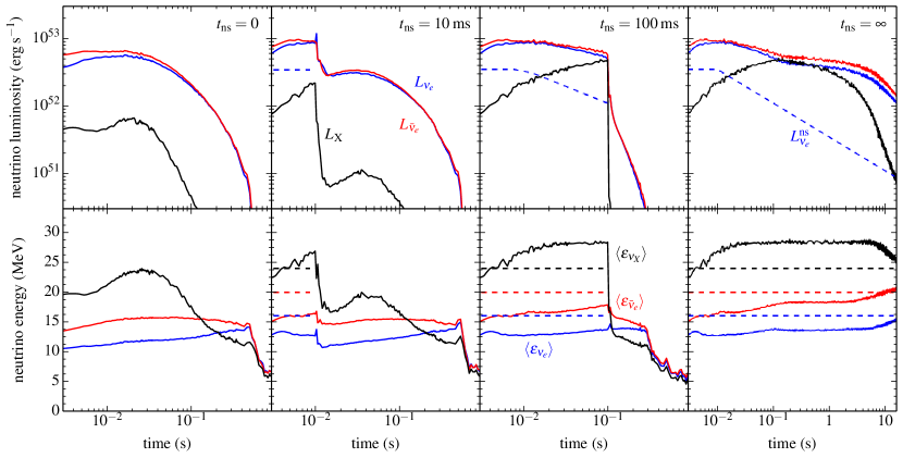
Figure 1: Neutrino luminosities emitted by the disk (top) and associated mean neutrino energies (bottom) in models without neutrino flavor transformation ($a_{\rm osc}=b_{\rm osc}=0$) and various HMNS lifetimes $t_{\rm ns}$, as labeled (corresponding, from left to right, to models bh-ab00, t010-ab00, t100-ab00, and tinf-ab00 in Table 1). The dashed lines show the imposed luminosity (Equation 6) and neutrino energies at the surface of the HMNS, when present. Note that the disk luminosities used in Equation (3) are corrected for global absorption, and are thus lower than those shown here (c.f. §III.2.2).

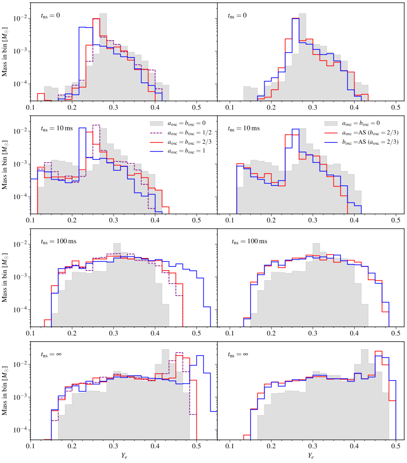
Figure 2: Mass histograms of electron fraction for unbound ejecta reaching $r=10^{9}$ cm by the end of each simulation ($t\simeq 17.7$ s). Rows from top to bottom show groups of models with different HMNS lifetime $t_{\rm ns}$, as labeled. The gray shaded histograms show models without flavor transformation, while colored curves show different combinations of flavor transformation coefficients $\{a_{\rm osc},b_{\rm osc}\}$ (see §II.2 for definitions): runs with symmetric coefficients ($a_{\rm osc}=b_{\rm osc}$) are on the left column, and asymmetric combinations on the right column. The bin width is $\Delta Y_{e}\simeq 0.017$.

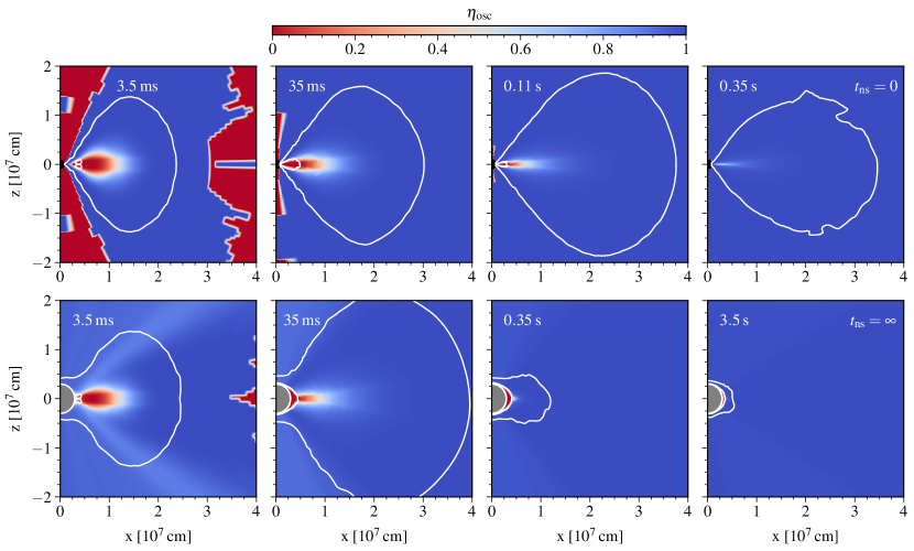
Figure 3: Activation parameter $\eta_{\rm osc}$ (Equation 9) that describes where we assume that the FFI operates, shown at selected times as labeled in the upper left corner of each panel (the rotation axis is along the $z$-axis and the equatorial plane is at $z=0$). The top row shows the prompt BH model with no flavor transformation (BH-ab00), while the bottom row shows the long-lived HMNS model with no flavor transformation (tinf-ab00). For the latter, we compute – in post-processing – an effective activation parameter that combines the contribution of disk and HMNS luminosities (Equation 15). The solid lines show density contours at $10^{8}$ g cm^-3 (outer) and $10^{11}$ g cm^-3 (inner). The black and gray circles indicate the size of the BH (absorbing) or HMNS (reflecting) boundary. The square-edged red region in the leftmost panels, and the cavity around the z-axis for the top row, corresponds to low-density ambient material where neutrino source terms are suppressed and we set $\eta_{\rm osc}=0$.

III.1 Overview of Evolution without Flavor Transformation

In order to analyze the effects of the FFI on the disk outflow, we first establish the baseline of comparison: accretion disks with variable HMNS lifetime that evolve without flavor transformation effects (model names ending in ‘ab00’). The initial maximum temperature and density in the torus are $7\times 10^{10}$ K ($\sim 6$ MeV) and $8\times 10^{10}$ g cm^-3, respectively, thus neutrino emission from the disk is significant, and the disk is optically thick in its densest regions (e.g., [14, 76]).

In the model with a promptly-formed BH (BH-ab00), the inner disk adjusts to a near-Keplerian spatial distribution over a few orbits at $r=50$ km (initial density peak radius), with neutrino emission peaking at $t\sim 20$ ms (top left panel of Figure 1). The emitted electron antineutrino luminosity is slightly larger than the electron neutrino luminosity, and both are about an order of magnitude larger than the combined heavy lepton luminosity. Neutrino emission evolves on a timescale set by viscous angular momentum transport, with luminosities dropping by a factor $\sim 100$ below their maximum at a time $t\sim 400$ ms. Thereafter, the disk is radiatively inefficient (e.g., [77]).

When a HMNS is present, a boundary layer forms at the surface of the star, and the disk can reach higher maximum densities and temperatures ($\sim 10^{12}$ g cm^-3 and $\sim 10^{11}$ K, respectively) than in the prompt BH case. This results in electron neutrino and antineutrino luminosities from the disk being higher by a factor of up to $\sim 2$ relative to the prompt BH case. For a long-lived HMNS (model tinf-ab00, top right panel of Figure 1), disk luminosities decay much more slowly with time than both the prompt BH luminosities and the HMNS luminosities imposed at the boundary. The heavy lepton neutrino/antineutrino luminosity from the disk $L_{\rm X}$ is significantly higher in model tinf-ab00 than in model BH-ab00, rising to values within a factor of a few of the emitted electron neutrino and antineutrino luminosities from the disk at $t\sim 200$ ms.

The intermediate cases of a HMNS lasting for 10 ms (model t010-ab00) or 100 ms (model t100-ab00) show neutrino luminosities intermediate between the prompt BH and long-lived HMNS cases. In the model with $t_{\rm ns}=10$ ms, upon HMNS collapse, all luminosities drop sharply to a level below those of the prompt BH case at the same time, and then recover over a timescale $t\sim 100$ ms until they approximately match those from model BH-ab00. The model with $t_{\rm ns}=100$ ms is such that upon BH formation, all luminosities also drop sharply but never recover to the level of the prompt BH model. We attribute this difference to transport of angular momentum by the boundary layer when the HMNS is present. The chosen surface rotation period of $3$ ms corresponds to sub-Keplerian rotation at the stellar surface and also at the ISCO radius of the BH, thus material co-rotating with the star at its surface is not able to circularize upon BH formation, and the resulting disk has less matter at the same time than a torus that began evolving around a BH.

Before BH formation (and for $t\lesssim 100$ ms in models BH-ab00 and t010-ab00), the mean energy of heavy lepton neutrinos emitted by the disk is higher by up to a factor of $\sim 2$ than those of electron neutrinos and antineutrinos (bottom row of Figure 1). This hierarchy is due to the low opacity of heavy lepton neutrinos and the steeper temperature dependence of the primary mechanism that produces them ($e^{+}e^{-}$ pair annihilation). In all cases, the mean energies of electron antineutrinos emitted by the disk are 20-50% higher than the mean energies of electron neutrinos, with values becoming close to one another only before a sharp drop at $t\sim 0.5$ s. The drop in mean energies is a consequence of energy luminosities decreasing faster with time than number luminosities as the disk transitions to a radiatively inefficient state with lower temperature and density.

Due to enhanced neutrino irradiation and suppressed mass loss through the inner boundary, a longer HMNS lifetime correlates with more mass ejected as well as an overall higher average electron fraction and velocity of the unbound ejecta [49, 78, 56, 55, 79], which in turn translates into a lower yield of heavy $r$-process elements [80, 51, 81] (Table 1). Our model t010-ab00 has a slightly lower average $Y_{e}$ than the prompt BH model due to a relative increase in the ejecta with $Y_{e}<0.25$ material (Figure 2)

Mass ejection in our models is driven by neutrino energy deposition, viscous heating, and nuclear recombination. Neutrino-driven outflows operate on a timescale of $\gtrsim 10$ ms and are significant whenever a HMNS is present. In pure BH models, and also in late-time HMNS disks, mass is primarily ejected by a combination of viscous heating and nuclear recombination, operating on a timescale of few $100$ ms. Simulations that include MHD effects have additional mass ejection channels available in the form of magnetic stresses (Lorentz force) that eject matter on a $\sim$ ms timescale, providing a distinct component (e.g., [82, 45, 83, 84, 85]). The composition of this prompt disk outflow is sensitive to that of the disk upon formation (i.e., neutron-rich), since weak interactions do not operate for long enough to bring $Y_{e}$ toward its equilibrium value. The properties of this early magnetic-driven ejection component are also sensitive to the initial field geometry (e.g., [86, 72]). In models with a long-lived HMNS, magnetic stresses and/or neutrino absorption combine to launch a fast outflow (e.g., [87, 88, 89, 90, 91, 92]).

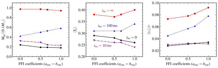
Figure 4: Average outflow properties as a function of flavor transformation intensity, parameterized through the FFI coefficients $\{a_{\rm osc},b_{\rm osc}\}$ in symmetric combinations ($a_{\rm osc}=b_{\rm osc}$, Table 1). Shown are the total unbound ejected mass (left), average electron fraction (middle), and average radial velocity (right), for various HMNS lifetimes $t_{\rm ns}$, as labeled in the middle panel.

III.2 Effect of Flavor Transformation on Outflow Properties

III.2.1 Overall Trends

Figure 3 shows the FFI activation parameter $\eta_{\rm osc}$ (Equation 9) for the prompt BH and long-lived HMNS models with $a_{\rm osc}=b_{\rm osc}=0$ at various times in the evolution. The BH disk starts optically thick in its denser regions and flavor transformation operates outside these opaque regions, by construction. For as long as neutrino emission remains significant, the disk retains a dense core where flavor transformation does not operate, while $\eta_{\rm osc}\sim 1$ in all the outflow material.

To diagnose the long-lived HMNS case, we compute an effective activation parameter (weighted by attenuated luminosity) that combines disk and stellar contributions (which are treated separately in our formalism, see §II.2):

$$\eta_{\rm osc}^{\rm(eff)}\equiv\frac{L^{*}_{\bar{\nu}_{e}}\,\eta_{\rm osc}^{2}+L^{\rm ns}_{\bar{\nu}_{e}}\,{\eta^{\rm ns}_{\rm osc}}^{2}}{L^{*}_{\bar{\nu}_{e}}\,\eta_{\rm osc}+L^{\rm ns}_{\bar{\nu}_{e}}\,\eta^{\rm ns}_{\rm osc}}.$$ (15)

This formulation implicitly neglects the difference between the distance to the HMNS surface and the disk emission ring, and assumes $\tau_{{\rm irr},\bar{\nu}_{e}}=\tau_{\bar{\nu}_{e}}$ (Equation 5). The disk optical depth is initially the same as in the BH case, but as accretion proceeds, a dense and neutrino-opaque boundary layer forms at the surface of the HMNS. Figure 3 shows that most of the disk and its outflow have nevertheless $\eta_{\rm osc}\sim 1$, which is due to the dominance of disk luminosities over HMNS luminosities (c.f., Figure 1). In fact, the opaque boundary layer prevents neutrinos emitted from the HMNS surface from reaching the disk, from the equator up to mid-latitude regions. Neutrino emission from the disk, on the other hand, is optically thin everywhere except the disk midplane at early times and the boundary layer, whenever present. This suggests that the effects of the FFI manifest primarily through disk luminosities on equatorial latitudes, while a mixture of both contributions acts along polar latitudes.

To quantitatively assess the effects of flavor transformation on our model set, we describe global outflow properties through quantities measured at an extraction radius $r_{\rm out}=10^{9}$ cm. The total ejected mass with positive Bernoulli parameter (Equation 1) reaching that radius over the course of the simulation is denoted by $M_{\rm ej}$, and the subset of this mass with $Y_{e}<0.25$ by $M_{\rm ej,red}$. The average electron fraction and radial velocity at $r_{\rm out}$ are weighted by the mass-flux (e.g., [48])

$$\langle Y_{e}\rangle = \frac{\int r_{\rm out}^{2}\rho v_{r}Y_{e}\,d\Omega\,dt}{\int r_{\rm out}^{2}\rho v_{r}\,d\Omega\,dt}$$ (16)

$$\langle v_{r}\rangle = \frac{\int r_{\rm out}^{2}\rho v_{r}^{2}\,d\Omega\,dt}{\int r_{\rm out}^{2}\rho v_{r}\,d\Omega\,dt},$$ (17)

where only matter with positive Bernoulli parameter is included in the integral, and the time range includes the entire simulation.

Table 1 shows that for each HMNS lifetime, the overall changes introduced by neutrino flavor transformation on the ejecta properties are moderate: at most $\sim 10\%$ in average electron fraction, up to $\sim 40\%$ in total ejecta mass, and $\sim 10-40\%$ in average velocity except for the most extreme FFI case with $t_{\rm ns}=100$ ms, for which it is a $73\%$ increase. The mass with $Y_{e}<0.25$ ($M_{\rm ej,red}$) can change by a factor of up to a few.

The direction of these changes depends on the HMNS lifetime, as illustrated by Figure 4 for models with symmetric FFI coefficients ($a_{\rm osc}=b_{\rm osc}$). For $t_{\rm ns}\leq 10$ ms, the average electron fraction of models with flavor transformation is always lower than in the un-oscillated case. Figure 2 illustrates the shift of the electron fraction distribution to more neutron-rich values, with the peak of mass ejection typically decreasing by up to $0.05$. A HMNS with lifetime $t_{\rm ns}\geq 100$ ms, on the other hand, shows an overall broadening of the $Y_{e}$ distribution when including flavor transformation, with the average electron fraction staying constant or increasing by at most $0.02$. The long-lived HMNS set shows a peak $Y_{e}$ value shifting to higher, proton-rich values.

In all cases, the average outflow velocity stays nearly constant or increases (most notably for $t_{\rm ns}=100$ ms) when including flavor transformation relative to the baseline case. Likewise, mass ejection decreases with a more intense FFI all in cases except for the set with $t_{\rm ns}=100$ ms.

For symmetric values of the oscillation coefficients (model names ending in ab00, ab05, ab07, and ab10), the magnitude of the changes introduced by flavor transformation generally varies monotonically with the value of these coefficients. The case $a_{\rm osc}=b_{\rm osc}=1$ shows the strongest effect, as expected. When using asymmetric coefficients, we find that the ratio of number luminosities in equation (14) starts low, since initially $N_{\nu_{e}}<N_{\bar{\nu_{e}}}$, but approaches values close to unity on a timescale of $\sim 35$ ms (10 orbits at $r=50$ km). The magnitude of the changes in average quantities is similar (but not always identical) to the case $a_{\rm osc}=b_{\rm osc}=2/3$, as expected. Differences between setting either $a_{\rm osc}$ or $b_{\rm osc}$ to asymmetric are minor, as shown by the right column of Figure 2.

Table 2: Average of quantities extracted from tracer particles. From left to right, the first 9 columns show model name, net change in $Y_{e}$ (eq. 23) , change in $Y_{e}$ due to emission/absorption of electron neutrinos/antineutrinos (eqns. 18-22, as labeled), net energy change due to viscous heating, neutrino emission/absorption, and alpha particle recombination (eqns. 24-26). For models with $t_{\rm ns}=10$ ms and $100$ ms, direct time integration of source terms (columns 2-9) is done from BH formation onward ($t_{\rm min}=t_{\rm ns})$. Likewise, for the long-lived HMNS model, integration begins at $t_{\rm min}=0$ but stops at $t_{\rm max}=35$ ms. Therefore, except for the prompt BH series, the net change in $Y_{e}$ in the second column does not capture the entire history, and comparisons should only be made between simulations with the same $t_{\rm ns}$. The last two columns show the average mass fraction of Lanthanides ($X_{\rm La}$) and Actinides ($X_{\rm Ac}$) obtained with SkyNet including the entire simulation, and extrapolating the trajectories to $30$ yr.

Model	$\Delta\bar{Y}^{\rm net}_{e}$	$\Delta\bar{Y}^{{\rm em},\nu_{e}}_{e}$	$\Delta\bar{Y}^{{\rm em},\bar{\nu}_{e}}_{e}$	$\Delta\bar{Y}^{{\rm abs},\nu_{e}}_{e}$	$\Delta\bar{Y}^{{\rm abs},\bar{\nu}_{e}}_{e}$	$\Delta\bar{q}_{\rm visc}$	$\Delta\bar{q}_{\nu}$	$\Delta\bar{q}_{\alpha}$	$\bar{X}_{\rm La}$	$\bar{X}_{\rm Ac}$
						($10^{19}$ erg g-1)			$(10^{-2})$	$(10^{-2})$
BH-ab00	0.19	1.05	0.96	0.44	0.16	2.06	-1.07	0.33	0.8	0.3
BH-ab05	0.18	1.03	0.99	0.34	0.12	2.13	-1.15	0.32	0.8	0.2
BH-ab07	0.17	1.08	1.06	0.30	0.11	2.31	-1.31	0.31	0.9	0.2
BH-ab10	0.16	1.09	1.12	0.20	0.08	2.60	-1.58	0.30	1.9	0.3
BH-aAS	0.17	1.04	1.06	0.25	0.11	2.43	-1.34	0.31	1.0	0.3
BH-bAS	0.17	1.08	1.07	0.30	0.13	2.36	-1.30	0.31	1.1	0.2
t010-ab00	0.11	0.69	0.58	0.32	0.10	1.39	-0.56	0.29	2.3	0.9
t010-ab05	0.10	0.63	0.57	0.22	0.07	1.50	-0.65	0.28	1.5	1.3
t010-ab07	0.09	0.59	0.56	0.17	0.05	1.52	-0.67	0.28	2.1	1.4
t010-ab10	0.07	0.57	0.58	0.08	0.03	1.67	-0.83	0.26	3.0	1.1
t010-aAS	0.09	0.54	0.54	0.14	0.05	1.44	-0.66	0.27	2.1	1.4
t010-bAS	0.09	0.61	0.59	0.18	0.06	1.63	-0.70	0.28	1.8	1.3
t010-L20	0.09	0.65	0.62	0.19	0.06	1.63	-0.76	0.28	1.8	1.4
t100-ab00	0.011	0.029	0.035	0.009	0.004	0.25	-0.04	0.13	0.6	0.08
t100-ab05	0.004	0.009	0.013	0.001	7E-4	0.14	-0.01	0.10	1.1	0.2
t100-ab07	0.002	0.006	0.008	6E-4	3E-4	0.09	-0.01	0.09	1.1	0.3
t100-ab10	0.001	0.004	0.005	3E-5	1E-5	0.06	-8E-3	0.07	1.1	0.2
t100-aAS	0.003	0.009	0.011	8E-4	4E-4	0.09	-0.02	0.09	1.2	0.3
t100-bAS	0.003	0.007	0.010	6E-4	4E-4	0.12	-0.01	0.09	1.2	0.3
t100-L20	0.003	0.010	0.013	9E-4	5E-4	0.11	-0.02	0.09	1.3	0.3
tinf-ab00	0.08	1.00	0.88	0.41	0.20	1.13	-1.79	0.02	0.5	0.2
tinf-ab05	0.08	1.02	0.90	0.40	0.19	1.09	-1.63	0.02	1.0	0.4
tinf-ab07	0.09	1.02	0.90	0.40	0.19	1.08	-1.52	0.02	0.9	0.4
tinf-ab10	0.11	1.06	0.90	0.43	0.17	1.07	-1.40	0.02	0.7	0.2
tinf-aAS	0.09	1.04	0.92	0.41	0.19	1.08	-1.47	0.02	1.0	0.4
tinf-bAS	0.09	1.01	0.90	0.40	0.19	1.09	-1.52	0.02	0.9	0.4
tinf-L20	0.09	1.05	0.91	0.44	0.21	1.09	-1.49	0.02	0.9	0.4
tinf-noT	0.07	1.00	0.87	0.37	0.17	1.15	-1.91	0.01	0.4	0.1

III.2.2 Physical Origin of the Changes due to the FFI

The effect of the FFI on the disk outflow can be ultimately traced back to the hierarchy of luminosities and energies shown in Figure 1. For the prompt BH case, where only neutrinos from the disk exist, flavor transformation through equations (10), (11), (12), and (13) replaces a high-luminosity, low-energy species ($\nu_{e}$, $\bar{\nu}_{e}$) for a low-luminosity, high-energy species ($\nu_{x}$, $\bar{\nu}_{x}$). In the optically-thin limit, neutrino number absorption is proportional to $\sim L_{\nu_{i}}\langle\epsilon_{\nu_{i}}\rangle$, with energy absorption having an an additional power of $\langle\epsilon_{\nu_{i}}\rangle$. In this simple picture, a complete flavor swap should decrease the electron-flavor neutrino luminosity by an order of magnitude and increase the average energy of electron-flavor neutrinos by a factor of up to $\sim 2$, for an overall decrease in number absorption of a factor of $\sim 2$.

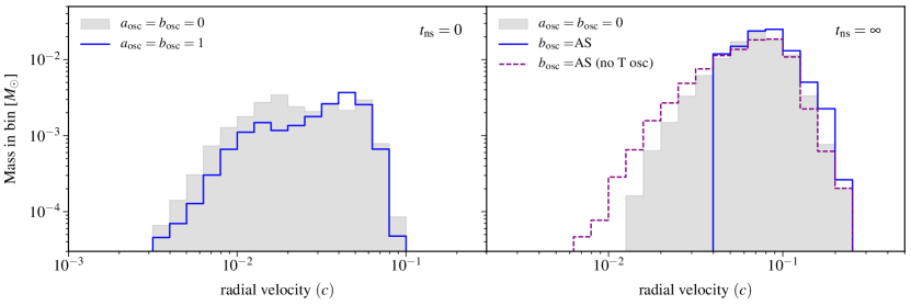
Figure 5: Mass histograms of radial velocity for unbound ejecta from selected simulations with a prompt BH (left) and long-lived HMNS (right), with flavor transformation coefficients as labeled. The dashed line on the right panel corresponds to the long-lived HMNS model with asymmetric $b_{\rm osc}$ but no mixing of the neutrino temperatures (model tinf-noT in Tables 1 and 2). The bin width is $\Delta\log(v_{r}/c)=0.1$.

To diagnose quantitatively the effects on the electron fraction, we show in Table 2 the time-integral of the source terms that control the evolution of $Y_{e}$ (c.f., [57]),

$$\Delta Y_{e}^{i}=\int_{t_{\rm min}}^{t_{\rm max}}\Gamma^{i}dt,$$ (18)

where $\Gamma^{i}$ is the rate per baryon of charged-current weak processes:

$$\Gamma^{\rm em,\nu_{e}}=\lambda_{e^{-}}Y_{p}: e^{-}+p\to n+\nu_{e}$$ (19)

$$\Gamma^{\rm em,\bar{\nu}_{e}}=\lambda_{e^{+}}Y_{n}: e^{+}+n\to p+\bar{\nu}_{e}$$ (20)

$$\Gamma^{\rm abs,\nu_{e}}=\lambda_{\nu_{e}}Y_{n}: \nu_{e}+n\to e^{-}+p$$ (21)

$$\Gamma^{\rm abs,\bar{\nu}_{e}}=\lambda_{\bar{\nu}_{e}}Y_{p}: \bar{\nu}_{e}+p\to e^{+}+n$$ (22)

where $\lambda_{i}$ are the reaction rates per target particle, and $Y_{n,p}$ the number of neutrons or protons per baryon (in the notation of [44]). Equation (18) is computed for each weak process in each trajectory that is unbound and reaches $r>10^{9}$ cm. Values are then averaged arithmetically over trajectories (which have identical mass for a given run), denoted by a bar above, and the net change is computed

$$\Delta\bar{Y}^{\rm net}_{e}=\Delta\bar{Y}^{\rm em,\bar{\nu}_{e}}_{e}-\Delta\bar{Y}^{\rm em,\nu_{e}}_{e}+\Delta\bar{Y}^{\rm abs,\nu_{e}}_{e}-\Delta\bar{Y}^{\rm abs,\bar{\nu}_{e}}_{e}.$$ (23)

The time range $[t_{\rm min},t_{\rm max}]$ in equation (18) is different for model sets with different HMNS lifetime. For the prompt BH case, the interval is the entire simulation time. For sets with $t_{\rm ns}=10$ ms and $100$ ms, the interval begins at BH formation ($t_{\rm min}=t_{\rm ns}$) and extends to the end of the simulation, because particles are created after HMNS collapse. For these model sets, quantities capture the impact of the FFI on post-collapse neutrino processes. For the long-lived HMNS case, the period extends from the start of the simulation ($t_{\rm min}=0$) until $10$ orbits at $r=50$ km ($t_{\rm max}\simeq 35$ ms). Limiting the integration interval is necessary because the absorption and emission terms in the long-lived HMNS case are large, and our trajectories are sampled at coarser time intervals at later times, leading to imprecise cancellation of large terms when numerically integrating over very long time intervals in post-processing. Because of this, direct comparisons should be made across models with the same $t_{\mathrm{ns}}$ in Table 2. Note that the tracer particles themselves are updated every time step and do not suffer from this post-processing error. In all cases, the chosen time interval satisfies $\bar{Y}_{e}(t_{\rm min})+\Delta\bar{Y}^{\rm net}_{e}=\bar{Y}_{e}(t_{\rm max})$.

The change in $Y_{e}$ with flavor transformation in the prompt BH models can be explained straightforwardly: as the FFI becomes stronger for models with increasing values of $a_{\rm osc}=b_{\rm osc}$, the average absorption of both electron neutrinos and antineutrinos decreases, with $\Delta\bar{Y}^{\rm abs,\nu_{e}}_{e}$ decreasing more than $\Delta\bar{Y}^{\rm abs,\bar{\nu}_{e}}_{e}$, with a maximum drop in absorption of a factor $\sim 2$. Emission terms, on the other hand, change by a few percent at most, since flavor transformation only changes emission rates indirectly through a minor effect on the disk dynamics. A decrease in neutrino absorption decreases the rate at which weak interactions bring $Y_{e}$ to its equilibrium value, and also lowers the equilibrium value itself (e.g., [84, 44]).

We diagnose the effects of flavor transformation on the outflow dynamics by integrating energy source terms of fluid elements. Table 2 shows the average specific energy gain of disk outflow trajectories through the quantities

$$\Delta q_{\rm visc} = \int_{t_{\rm min}}^{t_{\rm max}}\dot{q}_{\rm visc}dt$$ (24)

$$\Delta q_{\nu} = \int_{t_{\rm min}}^{t_{\rm max}}\dot{q}_{\rm\nu}dt$$ (25)

$$\Delta q_{\alpha} = \frac{B_{\alpha}}{m_{\alpha}}\left[X_{\alpha}(t_{\rm max})-X_{\alpha}(t_{\rm min})\right],$$ (26)

where $\dot{q}_{\rm visc}$ and $\dot{q}_{\rm\nu}$ are the rate of viscous and net neutrino heating per unit mass, respectively, ${B_{\alpha}}/{m_{\alpha}}$ is the nuclear binding energy per unit mass of alpha particles, and $X_{\alpha}$ is the mass fraction of alpha particles. For each model, the time range and particle sample employed is the same as in equation (18).

For the prompt BH models, the overall decrease in the neutrino absorption to emission ratio due to flavor transformation also results in higher net cooling of the torus (more negative $\Delta\bar{q}_{\nu}$), decreasing the vertical extent of the disk. This is accompanied by an increase in viscous heating, which is proportional to the local disk pressure (c.f., [48]). In the BH model with Complete flavor transformation (BH-ab10), net neutrino cooling increases by $60\%$ while viscous heating increases by $30\%$ relative to the Baseline model (BH-ab00). The left panel of Figure 5 shows the velocity distribution of the outflow from both models: the high-velocity portion of the histogram remains at a similar level, with flavor transformation inducing a slight shift to higher velocities of the peak, and a sizable decrease in the low velocity portion. If we change the unbinding criterion from Bernoulli to positive escape velocity, we find that the amount of mass ejected in model BH-ab10 is $10\%$ higher than in model BH-ab00, versus $25\%$ lower if we use the default Bernoulli criterion. Thus, the overall change in energy source terms introduced by the FFI in BH disks results in less marginally unbound mass ejected.

Regarding the long-lived HMNS model set (tinf), Table 2 shows that absorption of electron neutrino number slightly increases or stays constant in models with increasing $a_{\rm osc}=b_{\rm osc}$ in the first $35$ ms of evolution, while absorption of electron antineutrino number decreases in a similar way as in the pure BH case. A decrease in electron antineutrino absorption relative to neutrino absorption, with little change in the emission terms, increases the equilibrium value toward which $Y_{e}$ is driven (e.g., [84]).

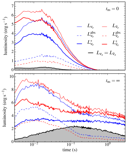
Figure 6: Luminosities as a function of time for the prompt BH model (top) and HMNS model (bottom) without flavor transformation. Shown for electron neutrinos and antineutrinos are the emitted luminosities $L_{\nu_{i}}$ (thin solid lines), total power absorbed $L_{\nu_{i}}^{\rm abs}$ (dashed lines), and net luminosities used in equation (3), $L_{\nu_{i}}^{*}=L_{\nu_{i}}-L_{\nu_{i}}^{\rm abs}$ (thick solid lines). The black lines show the emitted luminosities of heavy lepton neutrinos and antineutrinos, $L_{\nu_{x}}=L_{\bar{\nu}_{x}}=L_{\rm X}/2$ (we neglect their absorption so no correction is applied, i.e., $L_{\nu_{x}}^{*}=L_{\nu_{x}}$).

The increase in electron neutrino absorption with flavor transformation intensity for the long-lived HMNS is the consequence of two effects that modify the simpler picture for a prompt BH. First, the drop in electron neutrino luminosity upon flavor mixing is not as large as in the BH case. The heavy lepton luminosity is significantly larger than in the pure BH case, as the boundary layer region reaches higher densities and temperatures (Figure 1). Also, electron neutrino absorption is more important than in the pure BH case due to the opaque boundary layer. Figure 6 shows that the absorption-corrected luminosity $L_{\nu_{e}}^{*}$ is reduced relative to the emitted luminosity $L_{\nu_{e}}$ by a larger factor in model tinf-ab00 than in model BH-ab00 (for heavy leptons $L^{*}_{\rm X}=L_{\rm X}$ always, since we neglect their absorption). As a result, swapping $L^{*}_{\nu_{x}}$ and $L_{\nu_{e}}^{*}$ in the HMNS case results in a moderate (factor $\lesssim 2$) drop in electron neutrino flux during the relevant part of the evolution, in contrast to the BH case in which the decrease is a factor $\sim 10$.

The second effect leading to more electron neutrino absorption with flavor transformation in long-lived HMNS disks is the mixing of the temperature of emitted neutrinos (Equations 12-13). This effect is present in all models with flavor transformation, and it tends to increase net absorption by increasing the cross section, as the mean energy of heavy lepton neutrinos is always larger than that of electron neutrinos or antineutrinos (Figure 1). For the prompt BH models, this effect is sub-dominant, since the drop in neutrino flux is much larger than the increase in mean neutrino energies from the disk (c.f. Figure 6). For the long-lived HMNS case, however, the reduction in absorption rate due to the difference between $L_{\nu_{e}}^{*}$ and $L_{\nu_{x}}^{*}$ is comparable to or smaller than the increase in absorption rate from the increase in the absorption cross section due to the higher average neutrino energy. Thus, the global absorption of electron neutrinos remains nearly constant or even increases. More absorption of electron-type neutrinos increases the equilibrium electron fraction [84].

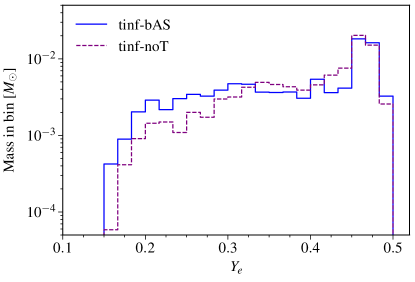
Figure 7: Mass histograms of electron fraction for unbound ejecta at the end of the simulation for a pair of long-lived HMNS models that differ only in that they either include (tinf-bAS, solid blue) or exclude (tinf-noT, dashed violet) mixing of the neutrino temperatures via Equations (12)-(13).

As a test of this interpretation, we ran another model (tinf-noT) with the same parameters as tinf-bAS but neglecting the swap of neutrino temperatures. The absorption of electron neutrinos then decreases during the first $35$ ms of evolution relative to model tinf-ab00 and tinf-bAS (Table 2) as expected, since $L_{\nu_{e}}^{*}$ is still larger than $L_{\nu_{x}}^{*}$ by a factor $\geq 2$ over that time period. The change in $Y_{e}$ over this interval is also smaller in model tinf-noT than in all other models with $t_{\rm ns}=\infty$.

Despite the lower amount of electron neutrino absorption in its early evolution and smaller change in $Y_{e}$, however, model tinf-noT has a higher average electron fraction by the end of the simulation (Table 1) than its sibling model that includes neutrino temperature oscillation (tinf-bAS). Figure 7 shows that while the peak of the electron fraction distribution by the end of the simulation is nearly the same in both cases, the amount of low $Y_{e}$ material is lower in model tinf-noT, hence the average over the entire outflow is higher.

To further dissect the origin of these changes, we note that Lippuner et al. [51] showed that the outflow from HMNS disks can be separated into an earlier, mostly neutrino-driven component, and a late component driven primarily by viscous heating and nuclear recombination. The early component exhibits a strong correlation between electron fraction and entropy, with a turnover in the range $Y_{e}\sim 0.4-0.5$, while the late component shows a more scattered distribution in entropy in a narrower $Y_{e}$ range. Figure 8 shows a scatter plot of unbound particles in $Y_{e}$-entropy-velocity space for models tinf-noT, tinf-bAS, and tinf-ab00, tagged by the time at which they reach the extraction radius at $r=10^{9}$ cm. The presence of the early ($t<1$ s, yellow) neutrino-driven wind component is evident, making up the majority of particles that span the electron fraction interval $[0.15,0.5]$ and forming the broad component of the $Y_{e}$ histogram in Figure 7. The smaller amount of of low-$Y_{e}$ ejecta from model tinf-noT is thus associated with a smaller contribution of the neutrino-driven wind, given the drop in luminosity upon flavor mixing without compensation by a higher neutrino temperature.

The late-time component is also evident in Figure 8 (blue particles), and is associated with the peak in the $Y_{e}$ histogram. The fact that this peak is at a similar value of $Y_{e}$ in models tinf-noT and tinf-bAS (Figure 7), but higher than the peak $Y_{e}$ from model tinf-ab00 (bottom right panel of Figure 2), indicates that its location is much more sensitive to the swapping of fluxes than to that of neutrino temperatures when the FFI operates. We can gain a qualitative understanding of these trends by evaluating the equilibrium electron fraction from pure absorption, to which a neutrino-driven wind without cooling is driven [93]

$$Y_{e}^{\rm eq,abs}\sim\left(1+\frac{\langle\varepsilon_{\bar{\nu}_{e}}\rangle\,L^{*}_{\bar{\nu}_{e}}}{\langle\varepsilon_{\nu_{e}}\rangle\,L^{*}_{\nu_{e}}}\right)^{-1}$$ (27)

where again we assume $\langle\epsilon_{\nu_{i}}^{2}\rangle=\langle\epsilon_{\nu_{i}}\rangle^{2}$. Ignoring attenuation, considering the contribution of the disk alone, and adopting constant $a_{\rm osc}=b_{\rm osc}=2/3$ we find $Y_{e}^{\rm eq,abs}\simeq\{0.35,0.39,0.45\}$ at $t=1$ s for models tinf-ab00, tinf-noT, and tinf-bAS, respectively. Considering the HMNS contribution alone, we get $Y_{e}^{\rm eq,abs}\simeq\{0.44,0.44,0.48\}$ independent of time for the same set of models. These values are consistent with model tinf-bAS having a more proton-rich $Y_{e}$ peak than the baseline model tinf-ab00, but do not fully account for model tinf-noT being closer to model tinf-bAS than to model tinf-ab00 in its late-time component. A spread in $Y_{e}$ within a given model can be accounted for by (1) latitude: particles ejected closer to the rotation axis have a stronger irradiation contribution from the HMNS, and (2) attenuation: fluctuations in the ratio of neutron to proton fraction alter the local incident luminosities in equation (27) though the optical depth, and thereby affect $Y_{e}^{\rm eq,abs}$. Also, neutrino emission is non-negligible, thus a more accurate value of the equilibrium electron fraction would include all four reactions contributing to the change in electron fraction (Equations 19-22) but is beyond the scope of this study.

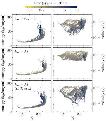
Figure 8: Entropy and radial velocity vs. electron fraction for unbound tracer particles from models with long-lived HMNS and different flavor transformation configuration: no FFI (tinf-ab00, top), asymmetric (tinf-bAS, middle) and asymmmetric with no neutrino temperature oscillation (tinf-noT, bottom). The color shows the time at which the particle last reaches $r=10^{9}$ cm.

Regarding mass ejected and average velocity of the long-lived HMNS outflow, Table 1 shows that when comparing model tinf-bAS with the unoscillated model (tinf-ab00), the average outflow velocity increases by $\sim 10\%$ while the mass ejected barely decreases ($\lesssim 2\%$). Removing the mixing of neutrino temperatures (model tinf-noT) results in a somewhat larger decrease in ejected mass ($3\%$) and a $5\%$ decrease in average velocity relative to the model without flavor transformation (tinf-ab00). Figure 5 shows the velocity histograms for these models: flavor transformation without oscillation of the neutrino temperatures produces more ejecta with low velocities, which is more weakly bound than matter that expands faster, for similar thermal energy content. We can attribute this to the lower absolute amount of absorption given the lower electron neutrino and antineutrino luminosities. Including temperature mixing increases neutrino absorption substantially, to the point that the low-velocity tail of the ejecta distribution is removed. Figure 8 shows that the missing low-velocity ejecta is primarily late-time, convective outflow that is more marginally unbound. This removal of low-velocity ejecta is also behind the trend of increasing average velocity with decreasing ejected mass for $t_{\rm ns}=\infty$ models with increasing $a_{\rm osc}=b_{\rm osc}$.

Regarding models with finite HMNS lifetime, the set with $t_{\rm ns}=10$ ms shows properties similar to the BH set. Tables 1 and 2 show that $65\%$ of the $Y_{e}$ change ($0.11/[\langle Y_{e}\rangle-Y_{e}(t=0)]$) occurs after BH formation for the unoscillated model (t010-ab00), following the same trend with FFI coefficients as the BH set. The same applies to the energy source terms post-BH formation: more viscous heating and net neutrino cooling, with nearly constant nuclear recombination heating.

The most notable difference with the prompt BH set is the bump in the electron fraction histogram at $Y_{e}\sim 0.1-0.2$ (Figure 2), which due to its similarity to models with longer HMNS lifetime, can be attributed to a more significant neutrino-driven component at early times. This bump decreases in magnitude and shifts to lower $Y_{e}$ with increasing FFI coefficients, in line with a weaker overall neutrino absorption level and a faster decrease of electron neutrino absorption than antineutrino absorption.

Regarding the model group with $t_{\rm ns}=100$ ms, Table 2 shows that very little change ($\sim 5\%$) in $Y_{e}$ occurs after BH formation, in line with the sharp decrease without recovery of the electron neutrino and antineutrino luminosities (Figure 1). The time integral of energy source terms also shows a very reduced importance of viscous heating and neutrino cooling, but a contribution of nuclear recombination that is only a factor $3$ lower than models for which the earlier phases are also computed ($t_{\rm ns}=0$ and $10$ ms). The evolution of this set of models is thus dominated by the earlier HMNS phase, during which neutrino absorption is a dominant process.

Comparing the $Y_{e}$ histograms of this set with those of the $t_{\rm ns}=\infty$ series (Figure 2) indicates that a neutrino-driven wind is clearly present, and becomes stronger with a more intense FFI. Figure 4 shows that $t_{\rm ns}=100$ ms is the only model set for which the ejected mass increases with more intense flavor transformation, which we interpret as neutrino absorption taking over as a driving mechanism of the outflow. We surmise that models with a long-lived HMNS saturate their mass ejection at nearly $>95\%$ of the initial disk mass, whereas the model set with $t_{\rm ns}=100$ ms has room to grow by starting at $42\%$ of the initial disk mass without FFI effects.

Finally, we find that our results have little sensitivity to the normalization of the heavy lepton luminosity imposed at the HMNS surface. Models t010-L20, t100-L20, and tinf-L20 have identical input parameters as the corresponding asymmetric models t010-bAS, t100-bAS, tinf-bAS, respectively (Table 1), except that we set $L_{\rm X,0}^{\rm ns}=2L_{\nu_{e},{\rm 0}}^{\rm ns}$ in equation (6). Comparing each pair of models with the same $t_{\rm ns}$ in Table 1 shows differences at the few percent level in all average quantities, with the exception of model t010-L20 which has an average velocity $10\%$ higher than model t010-bAS, and a mass with $Y_{e}<0.25$ that is a factor $\sim 2$ higher in the L20 case.

Table 2 shows that for this pair of models (t010-bAS and t010-L20), the main difference is that electron antineutrino emission after BH formation is higher in the model with enhanced heavy lepton HMNS luminosity, with a correspondingly higher net neutrino cooling. Looking at the tinf counterparts in Table 2, which share the first $10$ ms of evolution with the t010 models, we find a $10\%$ higher electron neutrino and antineutrino absorption in model tinf-L20 than in model tinf-bAS. While the net change in $Y_{e}$ is identical in this $35$ ms HMNS phase, the larger radiative driving can account for the higher average velocity in model t010-L20 relative to model t010-bAS. The larger amount of mass with $Y_{e}<0.25$ can be attributed to a more robust neutrino driven wind, which tends to launch more low-$Y_{e}$ ejecta at early times (Figure 8).

We expect the equilibrium $Y_{e}$ of the long-lived HMNS outflow to have an important dependency on the imposed electron neutrino and antineutrino luminosities at the HMNS boundary (normalization and time dependence, equation 6), since much of this radiation emitted toward equatorial latitudes is absorbed at the boundary layer, thus strongly influencing the $Y_{e}$ evolution in this region, which acts as a reservoir for the outflow. A more extended parameter space study, or a self-consistent HMNS and disk evolution, would be able to provide a more physically based characterization of the baseline $Y_{e}$ of a long-lived HMNS.

III.3 Nucleosynthesis Implications

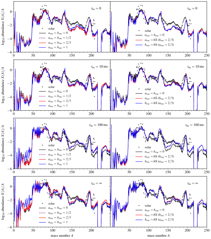
Figure 9: Final abundances at $t=30$ yr as a function of mass number, for unbound tracer particles from various models. Each row shows models with different HMNS lifetime, with left and right column showing models with symmetric and asymmetric flavor transformation coefficients, respectively. Circles show solar $r$-process abundances from [94], scaled to the abundance at $A=130$ from the model with no flavor transformation ($a_{\rm osc}=b_{\rm osc}=0$), for each value of $t_{\rm ns}$. Abundances are normalized such that all mass fractions $X(A)$ add up to unity.

Outflows from accretion disks are important contributors to the total ejecta from NS mergers, an example of which is GW170817, for which the disk ejecta is expected to have been dominant (e.g., [13, 95]). The abundance pattern of the ejecta thus has implications for the $r$-process enrichment contribution (e.g., [96, 97, 98, 99]) as well as on the kilonova signal through the opacities [100, 101, 102] and radioactive heating rates (e.g., [103, 104, 105, 106]). The $r$-process requires a high abundance of free neutrons when the ejecta temperature $T\lesssim 5\times 10^{9}$ K (e.g., [107]), which relates directly to the electron fraction of the ejecta shaped by neutrinos at earlier times when matter is hotter.

Figure 9 shows $r$-process abundances for trajectories from the same models shown in Figure 2. Overall, there are no qualitative changes in the abundance pattern for a given HMNS lifetime, regardless of the intensity of flavor transformation. More noticeable differences occur in models with larger $t_{\rm ns}$ due to the increasing protonization. The general trend is consistent with the $Y_{e}$ histograms: more intense flavor transformation produces more heavy $r$-process elements, and also more light elements (relative to $A\sim 130$) in models with a long-lived HMNS.

For a quantitative assessment, the average mass fraction of lanthanides $X_{\rm La}$ ($57\leq Z\leq 72$) and actinides $X_{\rm Ac}$ ($89\leq Z\leq 104$) are shown in Table 2 for all models. Overall, we see that flavor transformation induces at most a factor $\sim 2$ change in these mass fractions except for the model set with $t_{\rm ns}=100$ ms, which shows a larger variation in the actinide fraction relative to the unoscillated model. A more significant change of up to a factor of several in $M_{\mathrm{ej,red}}$ (mass ejected with $Y_{e}<0.25$) is seen in Table 1, which can alter the ratio of blue/red kilonovae light curves.

Our models suggest that the FFI introduces quantitative uncertainty in the disk outflow of at most a factor of two in the mass fraction of heavy $r$-process elements relevant to kilonova opacities, with minor changes to the overall $r$-process abundance pattern relative to the standard, no-FFI case.

III.4 Comparison with Previous Work

Li and Siegel [43] carried out GRMHD simulations of BH accretion disks using M1 neutrino transport. Their criterion to activate the FFI stems from a dispersion relation arising from the linearized evolution equation for neutrino flavor, with the FFI activated in regions with imaginary frequencies. Once activated, the FFI manifests as the equality of distribution functions of neutrinos ($f_{\nu_{e}}=f_{\nu_{\mu}}=f_{\nu_{\tau}}$) and antineutrinos, which is an equivalent assumption as used in our Flavor Equilibration case ($a_{\rm osc}=b_{\rm osc}=2/3$). In contrast to our models, however, mass ejection is dominated by magnetic stresses, since it takes several hundred milliseconds for the disk to reach the radiatively-inefficient stage where the outflow is driven (mostly) thermally. In this early phase of evolution, the initial composition of the disk is more important than for late-time outflows that were fully reprocessed by neutrinos. Consequently, their un-oscillated $Y_{e}$ distribution is much more neutron rich (peaking between $0.15$ and $0.2$) than that from our un-oscillated prompt BH model (Figure 2).

Given that baseline difference, however, introduction of the FFI produces very similar changes as in our prompt BH simulations. The $Y_{e}$ distribution shifts to more neutron-rich values by $0.01-0.02$, while the unbound mass ejected decreases by $\sim 10\%$. While the mass ejection mechanisms are different, this similarity stems from the fact that their FFI activation criterion results in widespread operation of the instability, similar to our $\eta_{\rm osc}$ parameter, and flavor swap should alter the emission terms (which dominate in the pure BH case) in the same way, making the disk more degenerate. Their $r$-process abundance pattern displays a larger enhancement in heavier elements when the FFI operates, given the larger relative amounts of ejecta with $Y_{e}<0.25$ than in our BH models.

Just et al. [44] performed axisymmetric viscous hydrodynamic simulations of BH accretion disks for a time $10$ s, as well as 3D MHD simulations for a time $0.5$ s, with an M1 neutrino scheme. The FFI is activated once the energy-averaged electron antineutrino flux factor (ratio of number flux to number density times $c$) exceeds a given value of $0.175$ by default, which corresponds to a layer below the neutrinosphere where angular asymmetries relevant to the FFI begin to appear according to a more detailed (static) analysis. The neutrinosphere is assumed to be at a flux factor of $1/3$, which in core-collapse supernovae corresponds to a radial optical depth of $2/3$ [41]. This activation criterion is very similar to our optical depth based parameter $\eta_{\rm osc}$ (Equation 9, Figure 3). Once active, the FFI is implemented by algebraically mixing the neutrino number densities and number fluxes of each flavor, separately for each energy bin of the multi-group M1 scheme. Three flavor mixing prescriptions are used, among which the assumptions behind their ‘mix2’ prescription are equivalent to our Flavor Equilibration case ($a_{\rm osc}=b_{\rm osc}=2/3$), while their ‘mix 1’ scheme that conserves net lepton number shares some similarities with our asymmetric scheme but is not equivalent.

Their baseline hydrodynamic simulation yields a similar ejecta mass, average velocity, and electron fraction distributions as our model bh-ab00. Their model that employs the ‘mix2’ scheme shows a $10\%$ decrease in ejecta mass and a decrease of the average electron fraction of $0.02$ relative to their baseline model, which follows the same trend as our models bh-ab07 compared to bh-ab00 (although we see a larger fractional ejecta mass decrease). Similar trends are found in their models that employ other mixing prescriptions. Unlike our models, however, the average velocity of all of their models that include the FFI decreases (by $10\%$ for the ‘mix2’ case) while in our corresponding models the average velocity shows an increase of $20\%$ when including the FFI. This discrepancy can be due to the way in which the average velocity is computed: mass-flux weighted at a fixed radius in our models (Equation 17) while density-weighted over a spatial region in theirs. It could also be due to the differences in absorption resulting from the different neutrino scheme, or the implementation of alpha viscosity and how viscous heating reacts to the increase in degeneracy from more efficient cooling due to the FFI. Their nucleosynthesis results are entirely consistent with ours.

Our long-lived HMNS model without flavor transformation is in overall qualitative agreement with that reported in [51], which used the same hydrodynamic setup but an older leakage scheme that considered only charged-current weak interactions, no heavy lepton neutrinos, and did not include an absorption correction to the disk luminosities. Quantitatively, comparing our Figure 8 to their Figure 3, the asymptotic $Y_{e}$ of their neutrino-driven wind ($\sim 0.55$) is higher than ours ($\sim 0.48$), and the peak $Y_{e}$ of their late component ($\sim 0.34$) is lower than what we find ($\sim 0.42$). Both models eject close to $100\%$ of the initial disk mass.

IV Summary and Discussion

We have studied the effect of the FFI on the long-term outflows from accretion disks around HMNSs of variable lifetime using axisymmetric, time-dependent, viscous hydrodynamic simulations. The instability is implemented parametrically into a 3-species leakage scheme for emission and a disk-lightbulb scheme for absorption by modifying the absorbed neutrino fluxes and temperatures. We explore a variety of cases, including partial and complete flavor equilibration, as well as an “asymmetric” flavor swap that reflects the conservation of lepton number in the neutrino self-interaction Hamiltonian. Our main results are the following:

1. – The impact of the FFI on the disk outflow is moderate, changing the total unbound mass ejected by up to $\sim 40\%$, the average electron fraction by $\sim 10\%$, and in most cases the average velocity by up to $\sim 40\%$ (Table 1, Figure 4). The lanthanide and actinide mass fractions of the outflow change, in most cases, by up to a factor of $\sim 2$ (Table 2), with no qualitative changes in the $r$-process abundance pattern for a given HMNS lifetime (Figure 9).

2. – The direction of the changes depends on the HMNS lifetime. For a promptly-formed BH or short-lived ($t_{\rm ns}\leq 10$ ms) HMNS, the mass ejected and average electron fraction decrease, and the average velocity increases. The composition changes can be traced back to a decrease in the electron neutrino/antineutrino absorption with FFI intensity (Table 2), which lowers the equilibrium $Y_{e}$ as well as the rate at which this equilibrium is reached (as previously found by [44] for prompt BH disks). The lesser absorption results in increased cooling, partially compensated by a higher viscous heating, with the net effect of lowering the entropy of the disk. A lower amount of ejected material with low velocities accounts for the decrease in mass ejected and higher average ejecta velocity (Figure 5).

3. – A longer-lived HMNS ($t_{\rm ns}\geq 100$ ms) displays a more significant role of neutrino absorption in driving the outflow (Figure 8). The FFI results in a more significant neutrino driven wind, broadening the electron fraction distribution, increasing the peak $Y_{e}$ to higher values (Figure 2), increasing the average velocity of the ejecta (Figure 5), and increasing the mass ejected up to a value of $\sim 95\%$ of the initial disk mass within $17.7$ s of evolution, for a very long-lived HMNS (Figure 4).

4. – The trends with HMNS lifetime can be traced back to the effects of flavor mixing by the FFI on the neutrino fluxes and temperatures. For BH disks, the heavy lepton luminosity is lower by a factor $\sim 10$ than the electron neutrino and antineutrino luminosity, while the mean energies of heavy leptons are higher by a factor $\sim 2$ (Figure 1). The net effect of flavor swap is to decrease absorption (more on electron neutrinos than antineutrinos) due to the change in neutrino flux (Table 2). For a HMNS disk, on the other hand, the heavy lepton luminosity is much higher than for a BH disk and the amount of electron neutrino reabsorption is significant, resulting in a very moderate change in the neutrino flux due to the FFI (Figure 6). The mixing of neutrino temperatures then results in a net increase in electron neutrino absorption (Table 2), with a protonization of the outflow as well as a more energetic neutrino-driven wind that ejects less low-velocity material (Figures 5 and 8).

5. – Despite the mild changes in composition, the total mass ejected with $Y_{e}<0.25$ can change by a factor of several (Table 1), thus altering the ratio of red to blue kilonova components if they are to be treated separately (e.g., due to spatial segregation).

Given the moderate impact of the FFI on the disk outflow, it is natural to think of this effect as introducing an uncertainty band to theoretical predictions for the ejecta properties. Our calculations corroborate other work [43, 44], indicating that an overall uncertainty of $\sim 10\%$ in ejected mass, electron fraction, and velocity, as well as a factor $2$ in lanthanide/actinide mass fraction can be used as a rule-of-thumb uncertainty in parameter inference from and/or upper limits on multi-messenger observations and galactic abundance studies (e.g., [108, 109, 110, 111, 112, 113, 114, 115, 116]). A similar uncertainty level is associated with spatial resolution of grid-based simulations of post-merger remnants (e.g., [48]). A more difficult task is to estimate uncertainties in kilonova light curves and spectra due to spatial segregation of lanthanide-rich vs lanthanide poor material, which would require radiative transfer simulations to assess the impact on the final outcome (e.g., [117, 118, 119]).

Our predictions can be made more reliable by (1) improving the quality of neutrino transport, in particular by using a spectral moment scheme to improve the angular distribution of radiation for the long-lived HMNS case; (2) self-consistently including the HMNS-disk system, avoiding the use of separate luminosities from each object; and (3) including magnetic fields in the evolution. The latter requires the use of three spatial dimensions, and the length of time required to fully capture the disk outflow makes such simulations computationally expensive, precluding an extensive parameter search with current capabilities. Selected flavor transformation scenarios will need to be carefully selected for those 3D GRMHD studies to augment the relatively small number of dynamical models performed to date.

Appendix A Derivation of the oscillation coefficients for the Asymmetric flavor transformation case

Neglecting collision terms in the quantum kinetic equation, the FFI arises from the neutrino self-interaction Hamiltonian

$$H_{\nu\nu}=\frac{\sqrt{2}G_{\rm F}}{(2\pi)^{3}}\int d^{3}p\,\left(f_{\nu}-\bar{f}_{\nu}^{*}\right)\left(1-\cos\theta\right)$$ (28)

where $f_{\nu}$ is the distribution function of species $\nu$, $\mathbf{p}$ is the neutrino momentum, $\theta$ the angle between the direction of the neutrino experiencing the potential and the momentum in the integrand, $G_{\rm F}$ is the Fermi constant, and we have assumed $h=c=1$ (e.g., [33]). Equation (28) satisfies $\bar{H}_{\nu\nu}=-H^{*}_{\nu\nu}$, which implies that the probability of flavor transformation is equal for neutrinos and antineutrinos propagating in the same direction. Integrating the quantum kinetic equation over neutrino direction, this symmetry implies conservation of net lepton number, which can be expressed as

$$n_{\nu_{e}}-n_{\nu_{x}}-n_{\bar{\nu}_{e}}+n_{\bar{\nu}_{x}}=\textrm{constant}.$$ (29)

Defining “oscillated” number densities as in Equations (10)-(11), we have

$$n^{\rm osc}_{\nu_{e}} = (1-a_{\rm osc})\,n_{\nu_{e}}+a_{\rm osc}\,n_{\nu_{x}}$$ (30)

$$n^{\rm osc}_{\nu_{x}} = (1-a_{\rm osc})\,n_{\nu_{x}}+a_{\rm osc}\,n_{\nu_{e}}$$ (31)

$$n^{\rm osc}_{\bar{\nu}_{e}} = (1-b_{\rm osc})\,n_{\bar{\nu}_{e}}+b_{\rm osc}\,n_{\bar{\nu}_{x}}$$ (32)

$$n^{\rm osc}_{\bar{\nu}_{x}} = (1-b_{\rm osc})\,n_{\bar{\nu}_{x}}+b_{\rm osc}\,n_{\bar{\nu}_{e}}.$$ (33)

Applying Equation (29)

$$n^{\rm osc}_{\nu_{e}}-n^{\rm osc}_{\nu_{x}}-n^{\rm osc}_{\bar{\nu}_{e}}+n^{\rm osc}_{\bar{\nu}_{x}}=n_{\nu_{e}}-n_{\nu_{x}}-n_{\bar{\nu}_{e}}+n_{\bar{\nu}_{x}},$$ (34)

and using $n_{\nu_{x}}=n_{\bar{\nu}_{x}}$, we obtain

$$a_{\rm osc}\left(n_{\nu_{e}}-n_{\nu_{x}}\right)=b_{\rm osc}\left(n_{\bar{\nu}_{e}}-n_{\bar{\nu}_{x}}\right),$$ (35)

which defines the Asymmetric flavor transformation case, and is the basis of Equation (14).

References

- Abbott et al. [2017] B. P. Abbott et al., ApJ 848, L12 (2017), arXiv:1710.05833 [astro-ph.HE] .
- Coulter et al. [2017] D. A. Coulter, R. J. Foley, C. D. Kilpatrick, M. R. Drout, A. L. Piro, B. J. Shappee, M. R. Siebert, J. D. Simon, N. Ulloa, D. Kasen, B. F. Madore, A. Murguia-Berthier, Y. C. Pan, J. X. Prochaska, E. Ramirez-Ruiz, A. Rest, and C. Rojas-Bravo, Science 358, 1556 (2017), arXiv:1710.05452 [astro-ph.HE] .
- Cowperthwaite et al. [2017] P. S. Cowperthwaite et al., ApJ 848, L17 (2017), arXiv:1710.05840 [astro-ph.HE] .
- Drout et al. [2017] M. R. Drout et al., Science 358, 1570 (2017), arXiv:1710.05443 [astro-ph.HE] .
- Tanaka et al. [2017] M. Tanaka et al., PASJ 69, 102 (2017), arXiv:1710.05850 [astro-ph.HE] .
- Tanvir et al. [2017] N. R. Tanvir et al., ApJ 848, L27 (2017), arXiv:1710.05455 [astro-ph.HE] .
- Lattimer and Schramm [1974] J. M. Lattimer and D. N. Schramm, The Astrophysical Journal 192, L145 (1974).
- Eichler et al. [1989] D. Eichler, M. Livio, T. Piran, and D. N. Schramm, Nature 340, 126 (1989).
- Freiburghaus et al. [1999] C. Freiburghaus, S. Rosswog, and F. Thielemann, ApJ 525, L121 (1999).
- Fernández and Metzger [2016] R. Fernández and B. D. Metzger, ARNPS 66, 23 (2016), arXiv:1512.05435 [astro-ph.HE] .
- Baiotti and Rezzolla [2017] L. Baiotti and L. Rezzolla, Reports on Progress in Physics 80, 096901 (2017).
- Radice et al. [2020] D. Radice, S. Bernuzzi, and A. Perego, Annual Review of Nuclear and Particle Science 70, 95 (2020).
- Shibata et al. [2017] M. Shibata, S. Fujibayashi, K. Hotokezaka, K. Kiuchi, K. Kyutoku, Y. Sekiguchi, and M. Tanaka, PRD 96, 123012 (2017), arXiv:1710.07579 [astro-ph.HE] .
- Ruffert et al. [1997] M. Ruffert, H.-T. Janka, K. Takahashi, and G. Schaefer, A&A 319, 122 (1997), arXiv:astro-ph/9606181 .
- Goodman et al. [1987] J. Goodman, A. Dar, and S. Nussinov, Astrophys. J. 314, L7 (1987).
- Richers et al. [2015] S. Richers, D. Kasen, E. O’Connor, R. Fernández, and C. D. Ott, ApJ 813, 38 (2015), arXiv:1507.03606 [astro-ph.HE] .
- Just et al. [2016] O. Just, M. Obergaulinger, H.-T. Janka, A. Bauswein, and N. Schwarz, ApJ 816, L30 (2016), arXiv:1510.04288 [astro-ph.HE] .
- Foucart et al. [2018] F. Foucart, M. D. Duez, L. E. Kidder, R. Nguyen, H. P. Pfeiffer, and M. A. Scheel, Phys. Rev. D 98, 063007 (2018), arXiv:1806.02349 [astro-ph.HE] .
- Fujibayashi et al. [2017] S. Fujibayashi, Y. Sekiguchi, K. Kiuchi, and M. Shibata, The Astrophysical Journal 846, 114 (2017).
- Sumiyoshi et al. [2021] K. Sumiyoshi, S. Fujibayashi, Y. Sekiguchi, and M. Shibata, Astrophys. J. 907, 92 (2021), arXiv:2010.10865 [astro-ph.HE] .
- Mikheyev and Smirnov [1989] S. P. Mikheyev and A. Y. Smirnov, Progress in Particle and Nuclear Physics 23, 41 (1989).
- Wolfenstein [1978] L. Wolfenstein, Physical Review D 17, 2369 (1978).
- Duan et al. [2010] H. Duan, G. M. Fuller, and Y.-Z. Qian, Annual Review of Nuclear and Particle Science 60, 569 (2010), arXiv:1001.2799 [hep-ph] .
- Mirizzi et al. [2016] A. Mirizzi, I. Tamborra, H.-T. Janka, N. Saviano, K. Scholberg, R. Bollig, L. Hüdepohl, and S. Chakraborty, La Rivista del Nuovo Cimento 39, 1 (2016).
- Capozzi and Saviano [2022] F. Capozzi and N. Saviano, Universe 8, 94 (2022).
- Malkus et al. [2016] A. Malkus, G. C. McLaughlin, and R. Surman, Phys. Rev. D 93, 045021 (2016), arXiv:1507.00946 [hep-ph] .
- Wu et al. [2016] M.-R. Wu, H. Duan, and Y.-Z. Qian, Physics Letters B 752, 89 (2016), arXiv:1509.08975 [hep-ph] .
- Wu and Tamborra [2017] M.-R. Wu and I. Tamborra, Phys. Rev. D 95, 103007 (2017), arXiv:1701.06580 [astro-ph.HE] .
- George et al. [2020] M. George, M.-R. Wu, I. Tamborra, R. Ardevol-Pulpillo, and H.-T. Janka, Phys. Rev. D 102, 103015 (2020), arXiv:2009.04046 [astro-ph.HE] .
- Bhattacharyya and Dasgupta [2020] S. Bhattacharyya and B. Dasgupta, Phys. Rev. D 102, 063018 (2020).
- Padilla-Gay et al. [2021] I. Padilla-Gay, S. Shalgar, and I. Tamborra, JCAP 2021 (1), 017, arXiv:2009.01843 [astro-ph.HE] .
- Wu et al. [2021] M.-R. Wu, M. George, C.-Y. Lin, and Z. Xiong, Phys. Rev. D 104, 103003 (2021), arXiv:2108.09886 [hep-ph] .
- Richers et al. [2021a] S. Richers, D. E. Willcox, N. M. Ford, and A. Myers, Phys. Rev. D 103, 083013 (2021a), arXiv:2101.02745 [astro-ph.HE] .
- Richers et al. [2021b] S. Richers, D. Willcox, and N. Ford, Phys. Rev. D 104, 103023 (2021b), arXiv:2109.08631 [astro-ph.HE] .
- Duan et al. [2021] H. Duan, J. D. Martin, and S. Omanakuttan, Physical Review D 104, 123026 (2021).
- Martin et al. [2021] J. D. Martin, J. Carlson, V. Cirigliano, and H. Duan, Physical Review D 103, 063001 (2021).
- Zaizen and Morinaga [2021] M. Zaizen and T. Morinaga, Physical Review D 104, 083035 (2021).
- Xiong et al. [2020] Z. Xiong, A. Sieverding, M. Sen, and Y.-Z. Qian, The Astrophysical Journal 900, 144 (2020).
- Sigl [2022] G. Sigl, Physical Review D 105, 043005 (2022).
- Richers et al. [2022] S. Richers, H. Duan, M.-R. Wu, S. Bhattacharyya, M. Zaizen, M. George, C.-Y. Lin, and Z. Xiong, arXiv e-prints , arXiv:2205.06282 (2022), arXiv:2205.06282 [astro-ph.HE] .
- Wu et al. [2017] M.-R. Wu, I. Tamborra, O. Just, and H.-T. Janka, Phys. Rev. D 96, 123015 (2017), arXiv:1711.00477 [astro-ph.HE] .
- Richers [2022] S. Richers, arXiv.2206.08444 10.48550/arXiv.2206.08444 (2022).
- Li and Siegel [2021] X. Li and D. M. Siegel, Phys. Rev. Lett. 126, 251101 (2021), arXiv:2103.02616 [astro-ph.HE] .
- Just et al. [2022a] O. Just, S. Abbar, M.-R. Wu, I. Tamborra, H.-T. Janka, and F. Capozzi, PRD, submitted , arXiv:2203.16559 (2022a), arXiv:2203.16559 [astro-ph.HE] .
- Fernández et al. [2019] R. Fernández, A. Tchekhovskoy, E. Quataert, F. Foucart, and D. Kasen, \mnras 482, 3373 (2019), arXiv:1808.00461 [astro-ph.HE] .
- Fryxell et al. [2000] B. Fryxell, K. Olson, P. Ricker, F. X. Timmes, M. Zingale, D. Q. Lamb, P. MacNeice, R. Rosner, J. W. Truran, and H. Tufo, ApJS 131, 273 (2000).
- Dubey et al. [2009] A. Dubey, K. Antypas, M. K. Ganapathy, L. B. Reid, K. Riley, D. Sheeler, A. Siegel, and K. Weide, J. Par. Comp. 35, 512 (2009).
- Fernández and Metzger [2013] R. Fernández and B. D. Metzger, MNRAS 435, 502 (2013), arXiv:1304.6720 [astro-ph.HE] .
- Metzger and Fernández [2014] B. D. Metzger and R. Fernández, \mnras 441, 3444 (2014), arXiv:1402.4803 [astro-ph.HE] .
- Fernández et al. [2015] R. Fernández, D. Kasen, B. D. Metzger, and E. Quataert, MNRAS 446, 750 (2015).
- Lippuner et al. [2017] J. Lippuner, R. Fernández, L. F. Roberts, F. Foucart, D. Kasen, B. D. Metzger, and C. D. Ott, MNRAS 472, 904 (2017), arXiv:1703.06216 [astro-ph.HE] .
- Artemova et al. [1996] I. V. Artemova, G. Bjoernsson, and I. D. Novikov, ApJ 461, 565 (1996).
- Shakura and Sunyaev [1973] N. I. Shakura and R. A. Sunyaev, A&A 24, 337 (1973).
- Timmes and Swesty [2000] F. X. Timmes and F. D. Swesty, ApJS 126, 501 (2000).
- Fahlman and Fernández [2018] S. Fahlman and R. Fernández, ApJ 869, L3 (2018), arXiv:1811.08906 [astro-ph.HE] .
- Fujibayashi et al. [2018] S. Fujibayashi, K. Kiuchi, N. Nishimura, Y. Sekiguchi, and M. Shibata, ApJ 860, 64 (2018), arXiv:1711.02093 [astro-ph.HE] .
- Fernández et al. [2020] R. Fernández, F. Foucart, and J. Lippuner, \mnras 497, 3221 (2020), arXiv:2005.14208 [astro-ph.HE] .
- Lippuner and Roberts [2017] J. Lippuner and L. F. Roberts, \apjs 233, 18 (2017), arXiv:1706.06198 [astro-ph.HE] .
- Cyburt et al. [2010] R. H. Cyburt, A. M. Amthor, R. Ferguson, Z. Meisel, K. Smith, S. Warren, A. e. Heger, R. D. Hoffman, T. Rauscher, A. e. Sakharuk, H. Schatz, F. K. Thielemann, and M. Wiescher, \apjs 189, 240 (2010).
- Frankel and Metropolis [1947] S. Frankel and N. Metropolis, Physical Review 72, 914 (1947).
- Mamdouh et al. [2001] A. Mamdouh, J. M. Pearson, M. Rayet, and F. Tondeur, \npa 679, 337 (2001), arXiv:nucl-th/0010093 [nucl-th] .
- Wahl [2002] A. C. Wahl, Technical Report LA-13928. Systematics of fission-product yields (Los Alamos National Laboratory, Los Alamos, NM, 2002).
- Panov et al. [2010] I. V. Panov, I. Y. Korneev, T. Rauscher, G. Martínez-Pinedo, A. Kelić-Heil, N. T. Zinner, and F. K. Thielemann, å 513, A61 (2010), arXiv:0911.2181 [astro-ph.SR] .
- Fuller et al. [1982] G. M. Fuller, W. A. Fowler, and M. J. Newman, \apjs 48, 279 (1982).
- Oda et al. [1994] T. Oda, M. Hino, K. Muto, M. Takahara, and K. Sato, Atomic Data and Nuclear Data Tables 56, 231 (1994).
- Langanke and Martínez-Pinedo [2000] K. Langanke and G. Martínez-Pinedo, \npa 673, 481 (2000), arXiv:nucl-th/0001018 [nucl-th] .
- Möller et al. [2016] P. Möller, A. J. Sierk, T. Ichikawa, and H. Sagawa, Atomic Data and Nuclear Data Tables 109, 1 (2016), arXiv:1508.06294 [nucl-th] .
- Ruffert et al. [1996] M. Ruffert, H.-T. Janka, and G. Schaefer, A&A 311, 532 (1996), arXiv:astro-ph/9509006 .
- Perego et al. [2016] A. Perego, R. M. Cabezón, and R. Käppeli, \apjs 223, 22 (2016), arXiv:1511.08519 [astro-ph.IM] .
- Ardevol-Pulpillo et al. [2019] R. Ardevol-Pulpillo, H. T. Janka, O. Just, and A. Bauswein, \mnras 485, 4754 (2019), arXiv:1808.00006 [astro-ph.HE] .
- Couch and O’Connor [2014] S. M. Couch and E. P. O’Connor, Astrophys. J. 785, 123 (2014), arXiv:1310.5728 [astro-ph.HE] .
- Fahlman and Fernández [2022] S. Fahlman and R. Fernández, \mnras 513, 2689 (2022), arXiv:2204.03005 [astro-ph.HE] .
- Fujibayashi et al. [2020] S. Fujibayashi, S. Wanajo, K. Kiuchi, K. Kyutoku, Y. Sekiguchi, and M. Shibata, Astrophys. J. 901, 122 (2020), arXiv:2007.00474 [astro-ph.HE] .
- Salpeter and Shapiro [1981] E. E. Salpeter and S. L. Shapiro, Astrophys. J. 251, 311 (1981).
- Janka [2001] H.-T. Janka, A&A 368, 527 (2001).
- Di Matteo et al. [2002] T. Di Matteo, R. Perna, and R. Narayan, ApJ 579, 706 (2002), arXiv:astro-ph/0207319 .
- Metzger et al. [2009] B. D. Metzger, A. L. Piro, and E. Quataert, MNRAS 396, 304 (2009), arXiv:0810.2535 .
- Perego et al. [2014] A. Perego, S. Rosswog, R. M. Cabezón, O. Korobkin, R. Käppeli, A. Arcones, and M. Liebendörfer, MNRAS 443, 3134 (2014), arXiv:1405.6730 [astro-ph.HE] .
- Fujibayashi et al. [2022] S. Fujibayashi, K. Kiuchi, S. Wanajo, K. Kyutoku, Y. Sekiguchi, and M. Shibata, ApJ, submitted , arXiv:2205.05557 (2022), arXiv:2205.05557 [astro-ph.HE] .
- Martin et al. [2015] D. Martin, A. Perego, A. Arcones, F. K. Thielemann, O. Korobkin, and S. Rosswog, Astrophys. J. 813, 2 (2015), arXiv:1506.05048 [astro-ph.SR] .
- Curtis et al. [2021] S. Curtis, P. Mösta, Z. Wu, D. Radice, L. Roberts, G. Ricigliano, and A. Perego, preprint , arXiv:2112.00772 (2021), arXiv:2112.00772 [astro-ph.HE] .
- Siegel and Metzger [2018] D. M. Siegel and B. D. Metzger, ApJ 858, 52 (2018), arXiv:1711.00868 [astro-ph.HE] .
- Miller et al. [2019] J. M. Miller, B. R. Ryan, J. C. Dolence, A. Burrows, C. J. Fontes, C. L. Fryer, O. Korobkin, J. Lippuner, M. R. Mumpower, and R. T. Wollaeger, Phys. Rev. D 100, 023008 (2019), arXiv:1905.07477 [astro-ph.HE] .
- Just et al. [2022b] O. Just, S. Goriely, H. T. Janka, S. Nagataki, and A. Bauswein, \mnras 509, 1377 (2022b), arXiv:2102.08387 [astro-ph.HE] .
- Hayashi et al. [2022] K. Hayashi, S. Fujibayashi, K. Kiuchi, K. Kyutoku, Y. Sekiguchi, and M. Shibata, Phys. Rev. D 106, 023008 (2022).
- Christie et al. [2019] I. M. Christie, A. Lalakos, A. Tchekhovskoy, R. Fernández, F. Foucart, E. Quataert, and D. Kasen, \mnras 490, 4811 (2019), arXiv:1907.02079 [astro-ph.HE] .
- Siegel et al. [2014] D. M. Siegel, R. Ciolfi, and L. Rezzolla, ApJ 785, L6 (2014), arXiv:1401.4544 [astro-ph.HE] .
- Ciolfi et al. [2019] R. Ciolfi, W. Kastaun, J. V. Kalinani, and B. Giacomazzo, Phys. Rev. D 100, 023005 (2019), arXiv:1904.10222 [astro-ph.HE] .
- Mösta et al. [2020] P. Mösta, D. Radice, R. Haas, E. Schnetter, and S. Bernuzzi, Astrophys. J. 901, L37 (2020), arXiv:2003.06043 [astro-ph.HE] .
- Shibata et al. [2021] M. Shibata, S. Fujibayashi, and Y. Sekiguchi, Phys. Rev. D 104, 063026 (2021), arXiv:2109.08732 [astro-ph.HE] .
- Most et al. [2021] E. R. Most, L. J. Papenfort, S. D. Tootle, and L. Rezzolla, \mnras 506, 3511 (2021), arXiv:2106.06391 [astro-ph.HE] .
- Sun et al. [2022] L. Sun, M. Ruiz, S. L. Shapiro, and A. Tsokaros, Phys. Rev. D 105, 104028 (2022), arXiv:2202.12901 [astro-ph.HE] .
- Qian and Woosley [1996] Y.-Z. Qian and S. E. Woosley, ApJ 471, 331 (1996), arXiv:astro-ph/9611094 .
- Goriely [1999] S. Goriely, A&A 342, 881 (1999).
- Metzger [2017] B. D. Metzger, Living Reviews in Relativity 20, 3 (2017), arXiv:1610.09381 [astro-ph.HE] .
- Rosswog et al. [2018] S. Rosswog, J. Sollerman, U. Feindt, A. Goobar, O. Korobkin, R. Wollaeger, C. Fremling, and M. M. Kasliwal, A&A 615, A132 (2018), arXiv:1710.05445 [astro-ph.HE] .
- Cowan et al. [2021] J. J. Cowan, C. Sneden, J. E. Lawler, A. Aprahamian, M. Wiescher, K. Langanke, G. Martínez-Pinedo, and F.-K. Thielemann, Reviews of Modern Physics 93, 015002 (2021), arXiv:1901.01410 [astro-ph.HE] .
- Shibata and Hotokezaka [2019] M. Shibata and K. Hotokezaka, Annual Review of Nuclear and Particle Science 69, 41 (2019), arXiv:1908.02350 [astro-ph.HE] .
- Siegel [2022] D. M. Siegel, Nature Reviews Physics 4, 306 (2022).
- Kasen et al. [2013] D. Kasen, N. R. Badnell, and J. Barnes, ApJ 774, 25 (2013), arXiv:1303.5788 [astro-ph.HE] .
- Tanaka and Hotokezaka [2013] M. Tanaka and K. Hotokezaka, ApJ 775, 113 (2013), arXiv:1306.3742 [astro-ph.HE] .
- Fontes et al. [2015] C. J. Fontes, C. L. Fryer, A. L. Hungerford, P. Hakel, J. Colgan, D. P. Kilcrease, and M. E. Sherrill, High Energy Density Physics 16, 53 (2015).
- Li and Paczyński [1998] L. Li and B. Paczyński, ApJ 507, L59 (1998).
- Metzger et al. [2010] B. D. Metzger, G. Martínez-Pinedo, S. Darbha, E. Quataert, A. Arcones, D. Kasen, R. Thomas, P. Nugent, I. V. Panov, and N. T. Zinner, MNRAS 406, 2650 (2010), arXiv:1001.5029 [astro-ph.HE] .
- Barnes et al. [2021] J. Barnes, Y. L. Zhu, K. A. Lund, T. M. Sprouse, N. Vassh, G. C. McLaughlin, M. R. Mumpower, and R. Surman, Astrophys. J. 918, 44 (2021), arXiv:2010.11182 [astro-ph.HE] .
- Klion et al. [2022] H. Klion, A. Tchekhovskoy, D. Kasen, A. Kathirgamaraju, E. Quataert, and R. Fernández, \mnras 510, 2968 (2022), arXiv:2108.04251 [astro-ph.HE] .
- Mendoza-Temis et al. [2015] J. d. J. Mendoza-Temis, M.-R. Wu, K. Langanke, G. Martínez-Pinedo, A. Bauswein, and H.-T. Janka, Phys. Rev. C 92, 055805 (2015), arXiv:1409.6135 [astro-ph.HE] .
- Kasliwal et al. [2020] M. M. Kasliwal et al., Astrophys. J. 905, 145 (2020), arXiv:2006.11306 [astro-ph.HE] .
- Thakur et al. [2020] A. L. Thakur et al., \mnras 499, 3868 (2020), arXiv:2007.04998 [astro-ph.HE] .
- Hernandez Vivanco et al. [2020] F. Hernandez Vivanco, R. Smith, E. Thrane, and P. D. Lasky, \mnras 499, 5972 (2020), arXiv:2008.05627 [astro-ph.HE] .
- Wanajo et al. [2021] S. Wanajo, Y. Hirai, and N. Prantzos, \mnras 505, 5862 (2021), arXiv:2106.03707 [astro-ph.GA] .
- Ricci et al. [2021] R. Ricci, E. Troja, G. Bruni, T. Matsumoto, L. Piro, B. O’Connor, T. Piran, N. Navaieelavasani, A. Corsi, B. Giacomazzo, and M. H. Wieringa, \mnras 500, 1708 (2021), arXiv:2008.03659 [astro-ph.HE] .
- Holmbeck et al. [2021] E. M. Holmbeck, A. Frebel, G. C. McLaughlin, R. Surman, R. Fernández, B. D. Metzger, M. R. Mumpower, and T. M. Sprouse, Astrophys. J. 909, 21 (2021), arXiv:2010.01621 [astro-ph.HE] .
- Raaijmakers et al. [2021] G. Raaijmakers, S. Nissanke, F. Foucart, M. M. Kasliwal, M. Bulla, R. Fernández, A. Henkel, T. Hinderer, K. Hotokezaka, K. Lukošiūtė, T. Venumadhav, S. Antier, M. W. Coughlin, T. Dietrich, and T. D. P. Edwards, Astrophys. J. 922, 269 (2021), arXiv:2102.11569 [astro-ph.HE] .
- Chen et al. [2021] H.-Y. Chen, S. Vitale, and F. Foucart, Astrophys. J. 920, L3 (2021), arXiv:2107.02714 [astro-ph.HE] .
- Gompertz et al. [2022] B. P. Gompertz, M. Nicholl, P. Schmidt, G. Pratten, and A. Vecchio, \mnras 511, 1454 (2022), arXiv:2108.10184 [astro-ph.HE] .
- Darbha and Kasen [2020] S. Darbha and D. Kasen, Astrophys. J. 897, 150 (2020), arXiv:2002.00299 [astro-ph.HE] .
- Korobkin et al. [2021] O. Korobkin, R. T. Wollaeger, C. L. Fryer, A. L. Hungerford, S. Rosswog, C. J. Fontes, M. R. Mumpower, E. A. Chase, W. P. Even, J. Miller, G. W. Misch, and J. Lippuner, Astrophys. J. 910, 116 (2021), arXiv:2004.00102 [astro-ph.HE] .
- Bulla et al. [2021] M. Bulla, K. Kyutoku, M. Tanaka, S. Covino, J. R. Bruten, T. Matsumoto, J. R. Maund, V. Testa, and K. Wiersema, \mnras 501, 1891 (2021), arXiv:2009.07279 [astro-ph.HE] .
- Loken et al. [2010] C. Loken, D. Gruner, L. Groer, R. Peltier, N. Bunn, M. Craig, T. Henriques, J. Dempsey, C.-H. Yu, J. Chen, L. J. Dursi, J. Chong, S. Northrup, J. Pinto, N. Knecht, and R. Van Zon, in Journal of Physics Conference Series, Journal of Physics Conference Series, Vol. 256 (2010) p. 012026.
- Ponce et al. [2019] M. Ponce, R. van Zon, S. Northrup, D. Gruner, J. Chen, F. Ertinaz, A. Fedoseev, L. Groer, F. Mao, B. C. Mundim, M. Nolta, J. Pinto, M. Saldarriaga, V. Slavnic, E. Spence, C.-H. Yu, and W. R. Peltier, arXiv e-prints , arXiv:1907.13600 (2019), arXiv:1907.13600 [cs.DC] .
- Hunter [2007] J. D. Hunter, Computing In Science & Engineering 9, 90 (2007).