TUM-HEP 1408/22

The first string-derived eclectic flavor model
with realistic phenomenology

Alexander Baur^a,b, Hans Peter Nilles^c, Saúl Ramos–Sánchez^b, Andreas Trautner^d,

and Patrick K.S. Vaudrevange^a *Electronic addresses

^aPhysik Department, Technische Universität München,
James-Franck-Straße 1, 85748 Garching, Germany

^bInstituto de Física, Universidad Nacional Autónoma de México,
POB 20-364, Cd.Mx. 01000, México

^cBethe Center for Theoretical Physics and Physikalisches Institut der Universität Bonn,
Nussallee 12, 53115 Bonn, Germany

^dMax-Planck-Institut für Kernphysik,
Saupfercheckweg 1, 69117 Heidelberg, Germany

Eclectic flavor groups arising from string compactifications combine the power of modular and traditional flavor symmetries to address the flavor puzzle. This top-down scheme determines the representations and modular weights of all matter fields, imposing strict constraints on the structure of the effective potential, which result in controlled corrections. We study the lepton and quark flavor phenomenology of an explicit, potentially realistic example model based on a $\mathbbm{T}^{6}/\mathbbm{Z}_{3}\times\mathbbm{Z}_{3}$ orbifold compactification of the heterotic string that gives rise to an $\Omega(2)$ eclectic flavor symmetry. We find that the interplay of flavon alignment and the localization of the modulus in the vicinity of a symmetry-enhanced point leads to naturally protected fermion mass hierarchies, favoring normal-ordered neutrino masses arising from a see-saw mechanism. We show that our model can reproduce all observables in the lepton sector with a small number of parameters and deliver predictions for so far undetermined neutrino observables. Furthermore, we extend the fit to quarks and find that Kähler corrections are instrumental in obtaining a successful simultaneous fit to the quark and lepton sectors.

1 Introduction

Top-down (TD) model building from string theory leads to the concept of the eclectic flavor group [1, 2, 3, 4] that includes traditional and modular flavor symmetries in the framework of “Local Flavor Unification” [5, 6]. Any discussion of the flavor problem should consider both, traditional and modular flavor symmetries, as they give important restrictions on the Kähler potential and superpotential of the theory. Spontaneous breaking of the eclectic flavor group exhibits a subtle interplay of the vacuum expectation values (VEVs) of flavon and moduli fields [7] that allow for a hierarchical pattern of masses and mixing angles of quarks and leptons. While the appearance of the eclectic flavor group is automatic in the TD approach, it could also be discussed within the bottom-up (BU) approach, where potential modular symmetries are contained in the outer automorphisms of the traditional flavor group [1, 5, 6]. In general, only part of the eclectic flavor group is linearly realized and the traditional flavor symmetry is enhanced at certain points or sub-loci in moduli space. This provides the basis of “Local Flavor Unification” at these regions of enhanced symmetry. Ultimately, this does lead to a flavor scheme that incorporates both the quark and lepton sectors.

Since their introduction in BU constructions [8], most of the attempts for a description of flavor with modular flavor symmetries have concentrated on the lepton sector alone, see e.g. [9, 10, 11, 12, 13, 14, 15, 16, 17, 18, 19, 20, 21, 22, 23] and references therein. Even though apparently more difficult to accomodate, there have been some fits of the flavor parameters that include the quark sector, see e.g. [24, 25, 26, 27, 28, 29, 30, 31, 32, 33, 34, 35, 36, 37]. Yet no clearly favored scheme has emerged. There are many choices of flavor groups, representations of these groups as well as parameters in the action that provide reasonable fits, but one still did not find a baseline theory or a fundamental principle through the BU considerations. Furthermore, the predictivity of these BU models may be challenged by the arbitrariness of their Kähler potential [38]. The TD approach is much more restrictive and it remains to be seen whether a realistic fit to the data can be achieved at all. The present paper is meant to be a first attempt for a global description of flavor in the quark and lepton sector from a TD perspective. It will also serve as a benchmark scheme that allows a comparison to previous BU constructions as it will indicate which properties of the construction and choice of parameters will be most relevant. We shall see, for example, that nontrivial parameters in the Kähler potential (usually ignored in the BU approach) might play an important role.

To initiate a TD construction of flavor we select a most promising scheme of a string compactification with an elliptic fibration based on the $\mathbbm{T}^{2}/\mathbbm{Z}_{3}$ orbifold [5, 2, 3]. It leads to the traditional flavor group $\Delta(54)$, the discrete modular flavor group $\Gamma^{\prime}_{3}\cong T^{\prime}=\mathrm{SL}(2,3)\cong[24,3]$ with eclectic flavor group $\Omega(2)\cong[1944,3448]$. Matter fields appear in twisted sectors with nontrivial representations of $\Delta(54)$ and $T^{\prime}$. Full details of this general flavor scheme can be found in table 2 of our previous paper [7]. The choice of the possible representations is quite restricted, as in other TD scenarios [39, 40, 41, 42]. It is therefore difficult to compare this approach to BU constructions where, even for the same group $T^{\prime}$, typically different representations have been chosen [15, 27, 35].

The next step in our program is the choice of a (semi-)realistic string construction with Standard Model gauge group $\mathrm{SU}(3)\times\mathrm{SU}(2)\times\mathrm{U}(1)$, three families of quarks and leptons and suitable Higgs-doublets. Here we concentrate on the constructions of ref. [43, 44] based on $\mathbbm{T}^{6}/\mathbbm{Z}_{3}\times\mathbbm{Z}_{3}$ orbifolds where the gauge and flavor structure has been explicitly worked out. Several classes of models with eclectic flavor group $\Omega(2)$ have been identified, as shown in table 3 of ref. [7]. We choose here the simplest example (class A) with properties displayed in table 1. Twisted fields all have the same modular weight $n=\nicefrac{{-2}}{{3}}$, transform as $\boldsymbol{3}_{2}$ representations of $\Delta(54)$ and $\boldsymbol{1}\oplus\boldsymbol{2}^{\prime}$ representations of the $T^{\prime}$ modular group. The pattern of the spontaneous breaking of the eclectic flavor group has been discussed in our earlier paper [7] (see Tables 1, 2 and 3 there). The simplicity of the scheme leads to severe restrictions on superpotential and Kähler potential as we shall discuss later in sections 2.4 and 2.5. Still, it has to be stressed that the Kähler potential is not diagonal (as usually assumed in the BU approach, with some exceptions [38, 27]) and this will be relevant for the global fit to the data.

The model allows for a successful fit of flavor both in the quark and lepton sector. It predicts a see-saw mechanism in the lepton sector and a “normal hierarchy” for neutrino masses. Hierarchies for masses and mixing angles appear from a subtle interplay of aligned flavon VEVs and the location of the modular parameter in the vicinity of fixed points, as a result of “Local Flavor Unification”.

The paper is structured as follows. In section 2 we present the explicit string model, matter representations (table 1), superpotential (section 2.4) and Kähler potential (2.5). Section 3 contains the step-wise symmetry breaking and the resulting hierarchical structure in a qualitative form. Section 4 will be devoted to the numerical analysis of the lepton sector, which will be completed to include also quarks in section 5. In section 6 we shall summarize our results and give an outlook to future developments. Our appendices include details on the structure of the Kähler corrections, our numerical analysis and the full massless matter spectrum of our model.

2 A string theory model with eclectic flavor symmetries

2.1 Model definition

	quarks and leptons						Higgs fields		flavons
label	$q$	$\bar{u}$	$\bar{d}$	$\ell$	$\bar{e}$	$\bar{\nu}$	$H_{\mathrm{u}}$	$H_{\mathrm{d}}$	$\varphi_{\mathrm{e}}$	$\varphi_{\mathrm{u}}$	$\varphi_{\nu}$	$\phi^{0}$	$\phi^{0}_{\mathrm{M}}$	$\phi^{0}_{\mathrm{e}}$	$\phi^{0}_{\mathrm{u}}$	$\phi^{0}_{\mathrm{d}}$
$\mathrm{SU}(3)_{c}$	$\boldsymbol{3}$	$\bar{\boldsymbol{3}}$	$\bar{\boldsymbol{3}}$	$\boldsymbol{1}$	$\boldsymbol{1}$	$\boldsymbol{1}$	$\boldsymbol{1}$	$\boldsymbol{1}$	$\boldsymbol{1}$	$\boldsymbol{1}$	$\boldsymbol{1}$	$\boldsymbol{1}$	$\boldsymbol{1}$	$\boldsymbol{1}$	$\boldsymbol{1}$	$\boldsymbol{1}$
$\mathrm{SU}(2)_{L}$	$\boldsymbol{2}$	$\boldsymbol{1}$	$\boldsymbol{1}$	$\boldsymbol{2}$	$\boldsymbol{1}$	$\boldsymbol{1}$	$\boldsymbol{2}$	$\boldsymbol{2}$	$\boldsymbol{1}$	$\boldsymbol{1}$	$\boldsymbol{1}$	$\boldsymbol{1}$	$\boldsymbol{1}$	$\boldsymbol{1}$	$\boldsymbol{1}$	$\boldsymbol{1}$
$\mathrm{U}(1)_{Y}$	$\nicefrac{{1}}{{6}}$	$-\nicefrac{{2}}{{3}}$	$\nicefrac{{1}}{{3}}$	$-\nicefrac{{1}}{{2}}$	$1$	$0$	$\nicefrac{{1}}{{2}}$	$-\nicefrac{{1}}{{2}}$	$0$	$0$	$0$	$0$	$0$	$0$	$0$	$0$
$\Delta(54)$	$\boldsymbol{3}_{2}$	$\boldsymbol{3}_{2}$	$\boldsymbol{3}_{2}$	$\boldsymbol{3}_{2}$	$\boldsymbol{3}_{2}$	$\boldsymbol{3}_{2}$	$\boldsymbol{1}$	$\boldsymbol{1}$	$\boldsymbol{3}_{2}$	$\boldsymbol{3}_{2}$	$\boldsymbol{3}_{2}$	$\boldsymbol{1}$	$\boldsymbol{1}$	$\boldsymbol{1}$	$\boldsymbol{1}$	$\boldsymbol{1}$
$T^{\prime}$	$\boldsymbol{2}^{\prime}\oplus\boldsymbol{1}$	$\boldsymbol{2}^{\prime}\oplus\boldsymbol{1}$	$\boldsymbol{2}^{\prime}\oplus\boldsymbol{1}$	$\boldsymbol{2}^{\prime}\oplus\boldsymbol{1}$	$\boldsymbol{2}^{\prime}\oplus\boldsymbol{1}$	$\boldsymbol{2}^{\prime}\oplus\boldsymbol{1}$	$\boldsymbol{1}$	$\boldsymbol{1}$	$\boldsymbol{2}^{\prime}\oplus\boldsymbol{1}$	$\boldsymbol{2}^{\prime}\oplus\boldsymbol{1}$	$\boldsymbol{2}^{\prime}\oplus\boldsymbol{1}$	$\boldsymbol{1}$	$\boldsymbol{1}$	$\boldsymbol{1}$	$\boldsymbol{1}$	$\boldsymbol{1}$
$\mathbbm{Z}_{9}^{R}$	$1$	$1$	$1$	$1$	$1$	$1$	$0$	$0$	$1$	$1$	$1$	$0$	$0$	$0$	$0$	$0$
$n$	$-\nicefrac{{2}}{{3}}$	$-\nicefrac{{2}}{{3}}$	$-\nicefrac{{2}}{{3}}$	$-\nicefrac{{2}}{{3}}$	$-\nicefrac{{2}}{{3}}$	$-\nicefrac{{2}}{{3}}$	$0$	$0$	$-\nicefrac{{2}}{{3}}$	$-\nicefrac{{2}}{{3}}$	$-\nicefrac{{2}}{{3}}$	$0$	$0$	$0$	$0$	$0$
$\mathbbm{Z}_{3}$	$1$	$1$	$\omega$	$\omega$	$1$	$1$	$1$	$1$	$1$	$\omega$	$\omega^{2}$	$1$	$1$	$\omega^{2}$	$\omega^{2}$	$\omega^{2}$
$\mathbbm{Z}_{3}$	$\omega^{2}$	$\omega^{2}$	$1$	$1$	$\omega^{2}$	$\omega^{2}$	$1$	$1$	$\omega^{2}$	$1$	$\omega$	$1$	$1$	$\omega^{2}$	$\omega^{2}$	$\omega^{2}$
$\mathbbm{Z}_{3}$	$1$	$1$	$\omega$	$1$	$1$	$1$	$1$	$1$	$1$	$\omega^{2}$	$1$	$1$	$1$	$1$	$\omega$	$\omega^{2}$

Table 1: MSSM matter and flavon states of a $\mathbbm{Z}_{3}$$\times$$\mathbbm{Z}_{3}$ heterotic orbifold realization of a model endowed with $\Omega(2)$ eclectic flavor symmetry. We display quantum numbers with respect to the SM gauge group, the traditional flavor symmetry $\Delta(54)$, the finite modular symmetry $T^{\prime}$, the modular weights $n$ and the $\mathbbm{Z}_{9}^{R}$ discrete $R$-symmetry arising from the full 10D orbifold compactification. We use the results from refs. [2, 4] to identify these quantum numbers. We provide the additional unbroken $\mathbbm{Z}_{3}\times\mathbbm{Z}_{3}\times\mathbbm{Z}_{3}$ symmetries (with $\omega:=e^{\nicefrac{{2\pi\mathrm{i}}}{{3}}}$), arising from the compact dimensions orthogonal to the $\mathbbm{T}^{2}/\mathbbm{Z}_{3}$ sector where $\Omega(2)$ is realized. As shown in appendix C, the fields carry additional gauge $\mathrm{U}(1)$ charges that distinguish e.g. $\phi^{0}$ and $\phi^{0}_{M}$. The subindices $\mathrm{e},\nu,\mathrm{u},\mathrm{d}$ label the flavons associated with the respective leptons and quarks. The electron and down-quark sectors share the same flavon triplet $\varphi_{\mathrm{e}}$, as discussed in section 2.4. Besides these relevant matter states, the model contains the vectorlike exotic fields shown in table 2.

Let us consider a fully consistent model based on the $\mathrm{E}_{8}$$\times$$\mathrm{E}_{8}$ heterotic string containing an eclectic flavor symmetry $\Omega(2)\cong[1944,3448]$, consisting of the traditional flavor group $\Delta(54)$, the finite modular group $T^{\prime}$ and a $\mathbbm{Z}_{9}^{R}$ $R$-symmetry. As usual, there is an additional $\mathbbm{Z}_{2}^{\mathcal{CP}}$ $\mathcal{CP}$-like modular symmetry that acts as a simultaneous outer automorphism on all of these groups and enlarges the eclectic flavor symmetry of this setting to order $3888$. The $\mathcal{CP}$-like transformation is generally spontaneously broken by the VEV of the modulus as well as by the VEVs of flavon fields thereby giving rise to $\mathcal{CP}$ violation at low energies. It has been known that $\mathbbm{T}^{6}/\mathbbm{Z}_{3}\times\mathbbm{Z}_{3}$ $(1,1)$ orbifold compactifications of the heterotic string with some vanishing Wilson lines can yield an MSSM-like massless spectrum equipped with a $\Delta(54)$ traditional flavor symmetry [46, 43, 44]. This symmetry arises from a two-dimensional $\mathbbm{T}^{2}/\mathbbm{Z}_{3}$ orbifold sector, whose modular symmetries complete the eclectic scenario [5, 6, 1, 2, 3, 4]. It leads to a picture where the $\Omega(2)$ eclectic symmetry of this sector is extended by three extra $\mathbbm{Z}_{3}$ symmetries arising from the other compact dimensions, which can be regarded as “shaping symmetries”.

We consider a particular string orbifold defined by the background gauge-lattice shifts

$$V_{1} = \left(-\tfrac{1}{2},\tfrac{1}{6},\tfrac{1}{6},\tfrac{1}{6},\tfrac{1}{6},\tfrac{1}{6},\tfrac{1}{6},\tfrac{1}{6}\right),\left(-\tfrac{1}{6},-\tfrac{1}{6},\tfrac{1}{6},\tfrac{1}{6},\tfrac{1}{6},\tfrac{1}{6},\tfrac{1}{2},\tfrac{7}{6}\right)\;,$$ (1a)

$$V_{2} = \left(-\tfrac{2}{3},-\tfrac{2}{3},-\tfrac{1}{3},0,0,0,1,\tfrac{4}{3}\right),\left(-\tfrac{5}{6},\tfrac{5}{6},\tfrac{1}{6},\tfrac{1}{6},\tfrac{1}{2},\tfrac{7}{6},-\tfrac{5}{6},\tfrac{5}{6}\right)\;,$$ (1b)

and Wilson lines

$$A_{1}=A_{2} = \left(-1,\tfrac{1}{3},-\tfrac{1}{3},-1,0,0,\tfrac{4}{3},-\tfrac{2}{3}\right),\left(\tfrac{3}{2},-\tfrac{1}{2},-\tfrac{1}{6},\tfrac{1}{2},\tfrac{5}{6},\tfrac{5}{6},-\tfrac{5}{6},-\tfrac{1}{6}\right)\;,$$ (1c)

$$A_{3}=A_{4} = \left(-\tfrac{1}{3},-\tfrac{2}{3},1,\tfrac{4}{3},\tfrac{1}{3},\tfrac{4}{3},\tfrac{2}{3},-1\right),\left(\tfrac{1}{2},\tfrac{1}{2},\tfrac{1}{2},\tfrac{1}{2},\tfrac{1}{2},\tfrac{3}{2},-\tfrac{1}{2},\tfrac{1}{2}\right)\;.$$ (1d)

The Wilson lines associated with the last two compact dimensions are chosen to be trivial, i.e. $A_{5}=A_{6}=0$. This is the condition for this $\mathbbm{T}^{2}/\mathbbm{Z}_{3}$ orbifold sector to yield the eclectic flavor symmetry $\Omega(2)$. One can further show that the three extra $\mathbbm{Z}_{3}$ discrete symmetries that are left unbroken from the orbifold action on the first four compact dimensions, are orthogonal to the $\Omega(2)$ eclectic group. From the gauge degrees of freedom, the unbroken 4D gauge group of this model is $\mathrm{SU}(3)_{c}\times\mathrm{SU}(2)_{L}\times\mathrm{U}(1)_{Y}\times[\mathrm{SU}(4)\times\mathrm{U}(1)^{9}]$. By using e.g. the orbifolder [47], one finds that the $\mathcal{N}=1$ massless matter spectrum includes three generations of quark and lepton superfields as well as a pair of Higgs fields and various flavons, all listed in table 1. Additionally, this model includes several vectorlike exotics summarized separately in table 2, which decouple from the low-energy dynamics when some singlets $s_{i}$ develop VEVs close to the string scale. Details of the entire massless spectrum are given in appendix C. We provide the SM gauge quantum numbers, as well as the discrete flavor charges for all phenomenologically relevant matter states in table 1, which we discuss in the following.

#	irrep	labels	#	irrep	labels
101	$\left(\boldsymbol{1},\boldsymbol{1}\right)_{0}$	$s_{i}$
51	$\left(\boldsymbol{1},\boldsymbol{1}\right)_{-\nicefrac{{1}}{{3}}}$	$V_{i}$	51	$\left(\boldsymbol{1},\boldsymbol{1}\right)_{\nicefrac{{1}}{{3}}}$	$\bar{V}_{i}$
14	$\left(\boldsymbol{1},\boldsymbol{1}\right)_{-\nicefrac{{2}}{{3}}}$	$X_{i}$	14	$\left(\boldsymbol{1},\boldsymbol{1}\right)_{\nicefrac{{2}}{{3}}}$	$\bar{X}_{i}$
10	$\left(\boldsymbol{1},\boldsymbol{2}\right)_{-\nicefrac{{1}}{{2}}}$	$L_{i}$	10	$\left(\boldsymbol{1},\boldsymbol{2}\right)_{\nicefrac{{1}}{{2}}}$	$\bar{L}_{i}$
9	$\left(\bar{\boldsymbol{3}},\boldsymbol{1}\right)_{\nicefrac{{1}}{{3}}}$	$\bar{D}_{i}$	9	$\left(\boldsymbol{3},\boldsymbol{1}\right)_{-\nicefrac{{1}}{{3}}}$	$D_{i}$
8	$\left(\boldsymbol{1},\boldsymbol{2}\right)_{-\nicefrac{{1}}{{6}}}$	$W_{i}$	8	$\left(\boldsymbol{1},\boldsymbol{2}\right)_{\nicefrac{{1}}{{6}}}$	$\bar{W}_{i}$
2	$\left(\bar{\boldsymbol{3}},\boldsymbol{1}\right)_{-\nicefrac{{2}}{{3}}}$	$\bar{U}_{i}$	2	$\left(\boldsymbol{3},\boldsymbol{1}\right)_{\nicefrac{{2}}{{3}}}$	$U_{i}$
4	$\left(\bar{\boldsymbol{3}},\boldsymbol{1}\right)_{0}$	$Z_{i}$	4	$\left(\boldsymbol{3},\boldsymbol{1}\right)_{0}$	$\bar{Z}_{i}$
1	$\left(\bar{\boldsymbol{3}},\boldsymbol{1}\right)_{-\nicefrac{{1}}{{3}}}$	$Y$	1	$\left(\boldsymbol{3},\boldsymbol{1}\right)_{\nicefrac{{1}}{{3}}}$	$\bar{Y}$

Table 2: Vectorlike exotic matter states of a $\mathbbm{Z}_{3}$$\times$$\mathbbm{Z}_{3}$ heterotic orbifold realization of a model endowed with $\Omega(2)$ eclectic flavor symmetry. In parenthesis, we display the gauge quantum number under $\mathrm{SU}(3)_{c}\times\mathrm{SU}(2)_{L}$ and the subindices denote the hypercharges.

2.2 Flavor symmetry representations

This model belongs to the category A of the models classified in table 3 of ref. [7]. The assignment of symmetry representations under the $\Omega(2)$ eclectic flavor symmetry is fairly simple because it is entirely determined by the modular weight $n$ of each field under the $\mathrm{SL}(2,\mathbbm{Z})_{T}$ group of modular transformations of the Kähler modulus $T$ [7]. We follow the notation of [2] and denote generic fields by $\Phi_{n}$ to indicate their transformation behavior under $\Omega(2)$. Quarks, leptons, and flavons $\varphi_{\mathrm{u},\mathrm{e},\nu}$ correspond to $\Phi_{\nicefrac{{-2}}{{3}}}$ fields with modular weights $n=\nicefrac{{-2}}{{3}}$, while the Higgs fields and flavons $\phi^{0}$ form $\Phi_{0}$ fields with trivial modular weights. While $\Phi_{0}$ fields are trivial singlets under all flavor symmetries, $\Phi_{\nicefrac{{-2}}{{3}}}$ are flavor triplets transforming simultaneously as $\boldsymbol{3}_{2}$ of the traditional flavor group $\Delta(54)$, as well as $\boldsymbol{2^{\prime}}\oplus\boldsymbol{1}$ of the finite modular group $T^{\prime}$ [6, 5]. In addition, $\Phi_{\nicefrac{{-2}}{{3}}}$ fields have $\mathbbm{Z}_{9}^{R}$-charge $1$ [4].

Next to the expectation value of the modulus $\langle T\rangle$ also the VEVs of the flavon triplets $\varphi_{\mathrm{i}}$ contribute to the breaking of the flavor symmetries of the model leading to the patterns described in our previous work [7].

The generators of the three-dimensional representation $\boldsymbol{3}_{2}$ of the traditional $\Delta(54)$ flavor symmetry are given by the matrices

$$\rho_{\boldsymbol{3}_{2}}(\mathrm{A})~{}:=~{}\left(\begin{array}[]{ccc}0&1&0\\ 0&0&1\\ 1&0&0\end{array}\right)\;,\quad\rho_{\boldsymbol{3}_{2}}(\mathrm{B})~{}:=~{}\left(\begin{array}[]{ccc}1&0&0\\ 0&\omega&0\\ 0&0&\omega^{2}\end{array}\right)\quad\mathrm{and,}\quad\rho_{\boldsymbol{3}_{2}}(\mathrm{C})~{}:=~{}-\left(\begin{array}[]{ccc}1&0&0\\ 0&0&1\\ 0&1&0\end{array}\right),$$ (2)

where $\omega:=\exp(\nicefrac{{2\pi\mathrm{i}}}{{3}})$, such that for $g\in\Delta(54)$,

$$\Phi_{\nicefrac{{-2}}{{3}}}~{}\stackrel{{\scriptstyle g}}{{\longrightarrow}}~{}\rho_{\boldsymbol{3}_{2}}(g)\,\Phi_{\nicefrac{{-2}}{{3}}}\;.$$ (3)

Furthermore, the superpotential $\mathcal{W}$ transforms under $\mathrm{C}$ as $\mathcal{W}\stackrel{{\scriptstyle\mathrm{C}}}{{\rightarrow}}-\mathcal{W}$, such that the $\mathbbm{Z}_{2}$ subgroup of $\Delta(54)$ generated by $\mathrm{C}$ corresponds to an $R$-symmetry. This also implies that the superpotential transforms as a $\Delta(54)$ nontrivial singlet $\boldsymbol{1}^{\prime}$, see also [7, Table 2].

For modular transformations,

$$\gamma~{}=~{}\begin{pmatrix}a&b\\ c&d\end{pmatrix}~{}\in~{}\mathrm{SL}(2,\mathbbm{Z})_{T}\;,$$ (4)

the transformations of the relevant matter fields and the superpotential are given by

$$\Phi_{\nicefrac{{-2}}{{3}}}~{}\stackrel{{\scriptstyle\gamma}}{{\longrightarrow}}~{}(c\,T+d)^{\nicefrac{{-2}}{{3}}}\,\rho(\gamma)\,\Phi_{\nicefrac{{-2}}{{3}}}\qquad\mathrm{and}\qquad\mathcal{W}~{}\stackrel{{\scriptstyle\gamma}}{{\longrightarrow}}~{}(c\,T+d)^{-1}\,\mathcal{W}\;,$$ (5)

with explicit representation matrices for the generators $\mathrm{S}$ and $\mathrm{T}$ of the modular group

$$\rho(\mathrm{S})~{}:=~{}\frac{\mathrm{i}}{\sqrt{3}}\left(\begin{array}[]{ccc}1&1&1\\ 1&\omega^{2}&\omega\\ 1&\omega&\omega^{2}\end{array}\right)\qquad\mathrm{and}\qquad\rho(\mathrm{T})~{}:=~{}\left(\begin{array}[]{ccc}\omega^{2}&0&0\\ 0&1&0\\ 0&0&1\end{array}\right)\;.$$ (6)

The $\mathbbm{Z}_{9}^{R}$ $R$-symmetry generated by the sublattice rotation $\hat{\mathrm{R}}$ (see [4] for details) acts as

$$\Phi_{\nicefrac{{-2}}{{3}}}~{}\stackrel{{\scriptstyle\hat{\mathrm{R}}}}{{\longrightarrow}}~{}\exp(\nicefrac{{2\pi\mathrm{i}}}{{9}})\,\Phi_{\nicefrac{{-2}}{{3}}}\qquad\mathrm{and}\qquad\mathcal{W}~{}\stackrel{{\scriptstyle\hat{\mathrm{R}}}}{{\longrightarrow}}~{}\omega\,\mathcal{W}\;.$$ (7)

Finally, the $\mathbbm{Z}_{3}\times\mathbbm{Z}_{3}\times\mathbbm{Z}_{3}$ charges shown in table 1 can be understood by the localization of the fields in the compact dimensions orthogonal to the $\mathbbm{T}^{2}/\mathbbm{Z}_{3}$ orbifold sector, supporting the geometric intuition of the eclectic picture. For completeness, let us recall that the generator of the additional $\mathbbm{Z}_{2}^{\mathcal{CP}}$ $\mathcal{CP}$-like symmetry of our TD eclectic scenario acts on the modulus as $T\stackrel{{\scriptstyle\mathcal{CP}}}{{\longrightarrow}}-\bar{T}$ while mapping $\Phi_{\nicefrac{{-2}}{{3}}}\stackrel{{\scriptstyle\mathcal{CP}}}{{\longrightarrow}}\bar{\Phi}_{\nicefrac{{-2}}{{3}}}$ [6, 5], where bars denote complex conjugation (in agreement with results in the BU approach [53]).

2.3 $T^{\prime}$ modular forms

In order to determine the structure of the effective action of the model, let us recall the properties of the modular forms that are relevant to build the couplings among the matter fields of table 1. For the leading terms in the superpotential we only need the modular forms of level 3 and weight 1, which form a doublet representations of $\Gamma^{\prime}_{3}\cong T^{\prime}$ and can be expressed as [15, 2]

$$\hat{Y}^{(1)}(T)~{}=~{}\begin{pmatrix}\hat{Y}_{1}(T)\\ \hat{Y}_{2}(T)\end{pmatrix}~{}=~{}\begin{pmatrix}-3\sqrt{2}\,\frac{\eta^{3}(3\,T)}{\eta(T)}\\ 3\frac{\eta^{3}(3\,T)}{\eta(T)}+\frac{\eta^{3}(T/3)}{\eta(T)}\end{pmatrix}\;,$$ (8)

where $\eta(T)$ is the Dedekind $\eta$ function. Under a modular transformation $\gamma\in\mathrm{SL}(2,\mathbbm{Z})_{T}$, this transforms as

$$\hat{Y}^{(1)}(T)\stackrel{{\scriptstyle\gamma}}{{\longrightarrow}}(c\,T+d)\,\rho_{\boldsymbol{2}^{\prime\prime}}(\gamma)\,\hat{Y}^{(1)}(T)\;,$$ (9)

where $\rho_{\boldsymbol{2}^{\prime\prime}}(\gamma)$ denotes the $\boldsymbol{2}^{\prime\prime}$ representation of $T^{\prime}$, which can be generated by

$$\rho_{\boldsymbol{2}^{\prime\prime}}(\mathrm{S})~{}=~{}-\dfrac{\mathrm{i}}{\sqrt{3}}\begin{pmatrix}1&\sqrt{2}\\ \sqrt{2}&1\end{pmatrix}\qquad\mathrm{and}\qquad\rho_{\boldsymbol{2}^{\prime\prime}}(\mathrm{T})~{}=~{}\begin{pmatrix}\omega&0\\ 0&1\end{pmatrix}\;.$$ (10)

Using $q:=\exp\left(2\pi\mathrm{i}\,T\right)$, we will make use of the “$q$-expansion” of $\hat{Y}^{(1)}(T)$ given by

$$\hat{Y}_{1}(T)~{} =~{}-3\,\sqrt{2}\,q^{\nicefrac{{1}}{{3}}}\,(1+q+2q^{2}+2q^{4}+q^{5}+2q^{6}+q^{8}+2q^{9}+\dots)\;,$$ (11a)

$$\hat{Y}_{2}(T)~{} =~{}1+6q+6q^{3}+6q^{4}+12q^{7}+6q^{9}+\dots\;.$$ (11b)

From these expansions, the behavior of the modular forms for large $\operatorname{Im}T$ can be read off: $\hat{Y}_{2}(T)\to 1$ while $\hat{Y}_{1}(T)\to 0$. Hence, for large $\operatorname{Im}T$, the modular form of weight $1$ is hierarchically structured.

Let us mention here the appearance of an approximate accidental symmetry because of the special behavior of these modular forms under the transformations $T\rightarrow T+\nicefrac{{3}}{{4}}$ and $T\rightarrow T+\nicefrac{{3}}{{2}}$. Using

$$T\rightarrow T+\nicefrac{{3}}{{4}} :\quad q~{}\rightarrow~{}\exp\left(2\pi\mathrm{i}(T+\nicefrac{{3}}{{4}})\right)~{}=~{}-\mathrm{i}\,q\;,$$ (12a)

$$T\rightarrow T+\nicefrac{{3}}{{2}} :\quad q~{}\rightarrow~{}\exp\left(2\pi\mathrm{i}(T+\nicefrac{{3}}{{2}})\right)~{}=~{}-q\;,$$ (12b)

and the $q$-expansions of eqs. (11), we find the approximate transformations

$$T\rightarrow T+\nicefrac{{3}}{{4}}: \quad\begin{pmatrix}\hat{Y}_{1}(T)\\ \hat{Y}_{2}(T)\end{pmatrix}~{}\rightarrow~{}\begin{pmatrix}-\mathrm{i}\,\hat{Y}_{1}(T)\\ \hat{Y}_{2}(T)\end{pmatrix}+\mathcal{O}(q)\;,$$ (13a)

$$T\rightarrow T+\nicefrac{{3}}{{2}}: \quad\begin{pmatrix}\hat{Y}_{1}(T)\\ \hat{Y}_{2}(T)\end{pmatrix}~{}\rightarrow~{}\begin{pmatrix}-\hat{Y}_{1}(T)\\ \hat{Y}_{2}(T)\end{pmatrix}+\mathcal{O}(q)\;.$$ (13b)

These relations will be useful to interpret some of our phenomenological observations in section 4.

We note that, under the generator of the $\mathbbm{Z}_{2}^{\mathcal{CP}}$ $\mathcal{CP}$-like symmetry, both components of the modular form get complex conjugated, i.e.

$$T\stackrel{{\scriptstyle\mathcal{CP}}}{{\longrightarrow}}-\bar{T}:\qquad\hat{Y}^{(1)}(T)~{}\stackrel{{\scriptstyle\mathcal{CP}}}{{\longrightarrow}}~{}\hat{Y}^{(1)}(-\bar{T})~{}=~{}\left(\hat{Y}^{(1)}(T)\right)^{*}\,.$$ (14)

2.4 Superpotential and mass matrices

Respecting gauge invariance as well as the correct transformation behavior under the eclectic flavor symmetries of the model (see table 1), the effective superpotential to leading order in operator mass dimension is given by

$$\mathcal{W}~{}=~{}\hat{Y}^{(1)}(T)\left\{\phi^{0}\left[\phi^{0}_{\mathrm{u}}H_{\mathrm{u}}\bar{u}q\varphi_{\mathrm{u}}+\phi^{0}_{\mathrm{d}}H_{\mathrm{d}}\bar{d}q\varphi_{\mathrm{e}}+\phi^{0}_{\mathrm{e}}H_{\mathrm{d}}\bar{e}\ell\varphi_{\mathrm{e}}+H_{\mathrm{u}}\bar{\nu}\ell\varphi_{\nu}\right]+\phi^{0}_{\mathrm{M}}\bar{\nu}\bar{\nu}\varphi_{\mathrm{e}}\right\}\;,$$ (15)

where henceforth we use Planck units. Here, $\hat{Y}^{(1)}(T)$ are the modular forms discussed in section 2.3 and, for brevity, we do not include the symmetry invariant overall couplings of each term. Note that by plain effective-field-theory (EFT) power counting, the neutrino Majorana mass term induced by the flavon VEV is hierarchically larger than the Dirac masses for all other quarks and leptons. A see-saw mechanism is thus a prediction of the model. In addition, we remark that down-quark and charged-lepton Yukawa couplings, as well as the Majorana mass term, all are accompanied by the same flavon triplet $\varphi_{\mathrm{e}}$, suggesting that our model exhibits a particular kind of bottom-tau unification.

Owing to the highly constraining symmetries, all superpotential terms in eq. (15) have the generic structure

$$\Phi_{0}\dots\Phi_{0}\,\hat{Y}^{(1)}(T)\,\Phi^{1}_{\nicefrac{{-2}}{{3}}}\,\Phi^{2}_{\nicefrac{{-2}}{{3}}}\,\Phi^{3}_{\nicefrac{{-2}}{{3}}}\;,$$ (16)

where the triplets $\Phi_{\nicefrac{{-2}}{{3}}}^{1}$ and $\Phi_{\nicefrac{{-2}}{{3}}}^{2}$ denote SM matter fields, $\Phi_{\nicefrac{{-2}}{{3}}}^{3}$ is a flavon triplet, and the series of $\Phi_{0}$’s includes a varying number of flavon singlets and the MSSM Higgs fields. Considering that the superpotential must transform as a nontrivial singlet $\boldsymbol{1}^{\prime}$ of $\Delta(54)$, see [7, Table 2], the explicit form of each mass term can be written as [2, 4]

$$\left(\Phi^{1}_{\nicefrac{{-2}}{{3}}}\right)^{\mathrm{T}}~{}M(T,c,\Phi_{\nicefrac{{-2}}{{3}}}^{3})~{}\Phi^{2}_{\nicefrac{{-2}}{{3}}}\;,$$ (17)

where

$$M(T,c,\Phi_{\nicefrac{{-2}}{{3}}}^{3})~{}:=~{}c~{}\begin{pmatrix}\hat{Y}_{2}(T)\,X&-\dfrac{\hat{Y}_{1}(T)}{\sqrt{2}}\,Z&-\dfrac{\hat{Y}_{1}(T)}{\sqrt{2}}\,Y\\[6.0pt] -\dfrac{\hat{Y}_{1}(T)}{\sqrt{2}}\,Z&\hat{Y}_{2}(T)\,Y&-\dfrac{\hat{Y}_{1}(T)}{\sqrt{2}}\,X\\[6.0pt] -\dfrac{\hat{Y}_{1}(T)}{\sqrt{2}}\,Y&-\dfrac{\hat{Y}_{1}(T)}{\sqrt{2}}\,X&\hat{Y}_{2}(T)\,Z\end{pmatrix}\;.$$ (18)

Here, we have expressed the three components of the flavon triplet as $\Phi_{\nicefrac{{-2}}{{3}}}^{3}=(X,Y,Z)^{\mathrm{T}}$ and introduced $c$ to denote the overall coefficient of the terms.

As an example, let us illustrate here how the charged lepton mass matrix $M_{\mathrm{e}}$ obeys the general texture described by eq. (18). For the charged lepton sector we find the following term in the superpotential of eq. (15)

$$\mathcal{W}_{\mathrm{e}}~{}=~{}c_{\mathrm{e}}\,\phi^{0}\,\phi^{0}_{\mathrm{e}}\,H_{\mathrm{d}}\,\left(\hat{Y}^{(1)}(T)\,\bar{e}\,\ell\,\varphi_{\mathrm{e}}\right)_{\boldsymbol{1}^{\prime}}\;.$$ (19)

Here, we have explicitly included the symmetry-invariant overall coefficient $c_{\mathrm{e}}$, which we take as a free parameter because its direct determination by string computations is still beyond our reach. After inserting the VEV $v_{\mathrm{d}}$ of the $H_{\mathrm{d}}$ Higgs field as well as all flavon VEVs, the mass matrix is given by

$$M_{\mathrm{e}}~{}=~{}M(T,\Lambda_{\mathrm{e}},\langle{\tilde{\varphi}_{\mathrm{e}}}\rangle)\;,\qquad\text{with}\qquad\Lambda_{\mathrm{e}}~{}=~{}c_{\mathrm{e}}\,v_{\mathrm{d}}\,\langle{\phi^{0}}\rangle\,\langle{\phi^{0}_{\mathrm{e}}}\rangle\,\Lambda_{\varphi_{\mathrm{e}}}\;$$ (20)

denoting the overall global scale which, effectively, is the only dimensionful parameter of the mass matrix. Here we have introduced the dimensionless flavon triplet $\tilde{\varphi}_{\mathrm{e}}$ and its VEV, defined by

$$\varphi_{\mathrm{e}}~{}=:~{}\Lambda_{\varphi_{\mathrm{e}}}~{}\tilde{\varphi}_{\mathrm{e}}\qquad\text{with}\qquad\tilde{\varphi}_{\mathrm{e}}~{}:=~{}\left(\tilde{\varphi}_{\mathrm{e},1},\,\tilde{\varphi}_{\mathrm{e},2},\,1\right)^{\mathrm{T}}.$$ (21)

Without loss of generality, we can assume that the components of the (dimensionless) flavon triplet VEV have the hierarchical structure

$$0~{}\leq~{}|\langle{\tilde{\varphi}_{\mathrm{e},1}}\rangle|~{}\leq~{}|\langle{\tilde{\varphi}_{\mathrm{e},2}}\rangle|~{}\leq~{}1\;.$$ (22)

Likewise, the neutrino masses are determined by the superpotential terms

$$\mathcal{W}_{\nu}~{}=~{}c_{\mathrm{D}}\,\phi^{0}\,H_{\mathrm{u}}\,\left(\hat{Y}^{(1)}(T)\,\bar{\nu}\,\ell\,\varphi_{\nu}\right)_{\boldsymbol{1}^{\prime}}~{}+~{}c_{\mathrm{M}}\,\phi^{0}_{\mathrm{M}}\,\left(\hat{Y}^{(1)}(T)\,\bar{\nu}\,\bar{\nu}\,\varphi_{\mathrm{e}}\right)_{\boldsymbol{1}^{\prime}}\;,$$ (23)

where we have explicitly included the symmetry-invariant coefficients $c_{\mathrm{D}}$ and $c_{\mathrm{M}}$, and indicated that we have to take the $\Delta(54)$ nontrivial singlet contraction $\boldsymbol{1}^{\prime}$ of each term. $\mathcal{W}_{\nu}$ predicts a type-I see-saw mechanism for neutrino masses. Hence, the light neutrino mass matrix is given by

$$M_{\nu}~{}=~{}-\dfrac{1}{2}\,M_{\mathrm{D}}\,M_{\mathrm{M}}^{-1}\,M_{\mathrm{D}}^{\mathrm{T}}\;,$$ (24)

where

$$M_{\mathrm{D}}~{}=~{}M(T,\Lambda_{\mathrm{D}},\langle{\tilde{\varphi}_{\nu}}\rangle)\qquad\text{and}\qquad M_{\mathrm{M}}~{}=~{}M(T,\Lambda_{\mathrm{M}},\langle{\tilde{\varphi}_{\mathrm{e}}}\rangle)$$ (25)

are the Dirac and Majorana neutrino mass matrices which again follow the general form (18). Analogously to eq. (21), we have defined the dimensionless flavon triplet $\tilde{\varphi}_{\nu}$ through

$$\varphi_{\nu}~{}=:~{}\Lambda_{\varphi_{\nu}}~{}\tilde{\varphi}_{\nu}\qquad\text{with}\qquad\tilde{\varphi}_{\nu}~{}:=~{}\left(\tilde{\varphi}_{\nu,1},\,\tilde{\varphi}_{\nu,2},\,1\right)^{\mathrm{T}}\;.$$ (26)

From the structure of the superpotential contribution (23) and the see–saw neutrino masses (24), we see that the overall scale of the light neutrino mass matrix is given by

$$\Lambda_{\nu}~{}=~{}\dfrac{\Lambda_{\mathrm{D}}^{2}}{\Lambda_{\mathrm{M}}}~{}=~{}\dfrac{\left(c_{\mathrm{D}}\,v_{\mathrm{u}}\,\langle{\phi^{0}}\rangle\,\Lambda_{\varphi_{\nu}}\right)^{2}}{c_{\mathrm{M}}\,\langle{\phi^{0}_{\mathrm{M}}}\rangle\,\Lambda_{\varphi_{\mathrm{e}}}}\;,$$ (27)

where $v_{\mathrm{u}}$ stands for the VEV of the up-type Higgs $H_{\mathrm{u}}$.

In complete analogy with the charged-lepton sector, from the Yukawa couplings for the up and down-quark sectors, we find that the corresponding mass matrices follow the structure of eq. (18) depending as follows on the different parameters

$$M_{\mathrm{u}}~{} =~{}M(T,\Lambda_{\mathrm{u}},\langle{\tilde{\varphi}_{\mathrm{u}}}\rangle) \Lambda_{\mathrm{u}}~{}=~{}c_{\mathrm{u}}\,v_{\mathrm{u}}\,\langle{\phi^{0}}\rangle\,\langle{\phi^{0}_{\mathrm{u}}}\rangle\,\Lambda_{\varphi_{\mathrm{u}}}\;,$$ with (28a)

$$M_{\mathrm{d}}~{} =~{}M(T,\Lambda_{\mathrm{d}},\langle{\tilde{\varphi}_{\mathrm{e}}}\rangle) \Lambda_{\mathrm{d}}~{}=~{}c_{\mathrm{d}}\,v_{\mathrm{d}}\,\langle{\phi^{0}}\rangle\,\langle{\phi^{0}_{\mathrm{d}}}\rangle\,\Lambda_{\varphi_{\mathrm{e}}}\;.$$ with (28b)

Analogously to the previous cases, $c_{\mathrm{u}}$ and $c_{\mathrm{d}}$ denote the unconstrained symmetry-invariant coefficients of the up and down-quark Yukawa couplings, respectively. Furthermore,

$$\varphi_{\mathrm{u}}~{}=:~{}\Lambda_{\varphi_{\mathrm{u}}}~{}\tilde{\varphi}_{\mathrm{u}}\qquad\text{with}\qquad\tilde{\varphi}_{\mathrm{u}}~{}:=~{}\left(\tilde{\varphi}_{\mathrm{u},1},\,\tilde{\varphi}_{\mathrm{u},2},\,1\right)^{\mathrm{T}}\;.$$ (29)

In summary, the superpotential contributions to the lepton masses include the following parameters: the global mass scales $\Lambda_{\mathrm{e}}$ for charged leptons and $\Lambda_{\nu}$ for neutrinos, the VEV $\langle{T}\rangle$ of the complex Kähler modulus, and the free components, $\langle{\tilde{\varphi}_{\mathrm{e},1}}\rangle$, $\langle{\tilde{\varphi}_{\mathrm{e},2}}\rangle$, $\langle{\tilde{\varphi}_{\nu,1}}\rangle$ and $\langle{\tilde{\varphi}_{\nu,2}}\rangle$, of the flavon VEVs. As we shall see, a subtle interplay among the modulus and flavon VEVs can explain the observed lepton-mass hierarchies (cf. section 3.2) and even yield a fit of lepton flavor data with interesting predictions (cf. section 4). We will see that it suffices to consider real flavon VEVs to arrive at those results, which implies that the modulus VEV $\langle{T}\rangle$ is the only source of $\mathcal{CP}$ violation in the lepton sector. Finally, since we aim at a global fit of flavor in both lepton and quark sectors, note that up-quark Yukawa couplings introduce additional parameters: the global up and down-quark mass scales $\Lambda_{\mathrm{u}}$ and $\Lambda_{\mathrm{d}}$ as well as the flavon components $\langle{\tilde{\varphi}_{\mathrm{u},1}}\rangle$ and $\langle{\tilde{\varphi}_{\mathrm{u},2}}\rangle$. Down-quark Yukawas in the superpotential of our model, eq. (15), share the charged-lepton flavon $\tilde{\varphi}_{\mathrm{e}}$, avoiding extra parameters but also imposing thereby severe constraints. In fact, these restrictions challenge the compatibility of our model with observations. Fortunately, as we shall see in section 5, this issue can be addressed by including Kähler corrections, which we now discuss.

2.5 Kähler corrections to the mass matrices

In contrast to the most common assumption of BU model building, the Kähler potential is, in general, nontrivial. In string-derived TD models, we have to include the phenomenological consequences of this fact. At leading order in the EFT expansion of the matter fields and flavons, the Kähler potential of the model introduced in section 2.1 is given by [2]

$$K~{}\supset ~{}-\log(-\mathrm{i}T+\mathrm{i}\bar{T})$$ (30)

$$~{}+\sum_{\Psi}\left[(-\mathrm{i}T+\mathrm{i}\bar{T})^{\nicefrac{{-2}}{{3}}}+(-\mathrm{i}T+\mathrm{i}\bar{T})^{\nicefrac{{1}}{{3}}}|\hat{Y}^{(1)}(T)|^{2}\right]|\Psi|^{2}$$

$$~{}+\sum_{\varphi}\left[(-\mathrm{i}T+\mathrm{i}\bar{T})^{\nicefrac{{-2}}{{3}}}+(-\mathrm{i}T+\mathrm{i}\bar{T})^{\nicefrac{{1}}{{3}}}|\hat{Y}^{(1)}(T)|^{2}\right]|\varphi|^{2}\;.$$

Here we again suppress all symmetry-invariant coupling parameters, and the respective summations run over all MSSM matter fields, $\Psi\in\{q,\bar{u},\bar{d},\ell,\bar{e},\bar{\nu}\}$, and the various flavon triplets of the model, $\varphi\in\{\varphi_{\mathrm{e}},\varphi_{\mathrm{u}},\varphi_{\nu},\ldots\}$, see table 1. Interestingly, the canonical form of the Kähler potential at this level is preserved in models endowed with eclectic symmetries because matter fields are charged under a traditional flavor symmetry [2], $\Delta(54)$ in our case, avoiding the loss of predictivity that challenges models exclusively based on modular symmetries [38]. Consequently, corrections to this canonical Kähler potential only appear if the traditional flavor symmetry is spontaneously broken by flavons. Couplings between flavons and matter fields induce additional terms in the Kähler potential of the form

$$K~{}\supset~{}\sum_{\Psi,\varphi}\left[(-\mathrm{i}T+\mathrm{i}\bar{T})^{\nicefrac{{-4}}{{3}}}\sum_{a}|\Psi\varphi|^{2}_{\boldsymbol{1},a}+(-\mathrm{i}T+\mathrm{i}\bar{T})^{\nicefrac{{-1}}{{3}}}\sum_{a}|\hat{Y}^{(1)}(T)\Psi\varphi|^{2}_{\boldsymbol{1},a}\right]\;,$$ (31)

where the subindex ${\boldsymbol{1},a}$ refers to the $a$th invariant singlet contraction with respect to the whole eclectic flavor symmetry. Since the terms in eq. (31) are proportional to the ratio of flavon VEVs to the fundamental scale, they represent small corrections to the leading-order Kähler potential (30). For simplicity, we restrict ourselves here to the modular forms $\hat{Y}^{(1)}(T)$ that naturally appear also in the superpotential $\mathcal{W}$.

Since the (Planck suppressed) next-to-leading order terms, given in eq. (31), can yield noncanonical contributions if the flavons develop VEVs, let us briefly discuss the consequences of such contributions. As pointed out in [38], noncanonical terms can be relevant for the mass matrices of a model. Hence, studying the Kähler potential is important to correctly determine the phenomenology of a model. In order to canonically normalize the fields, the Kähler metric associated with $\Psi$

$$K_{ij}~{}=~{}\dfrac{\partial^{2}K}{\partial\Psi_{i}~{}\partial\Psi_{j}^{*}}$$ (32)

needs to be diagonalized, such that

$$K_{ij}~{}=~{}\left(U_{K}^{\dagger}\,D^{2}\,U_{K}\right)_{ij}\;,$$ (33)

where $U_{K}$ is unitary and $D$ is diagonal and positive. Then, the canonically normalized fields $\hat{\Psi}$ read

$$\hat{\Psi}~{}=~{}D\,U_{K}\,\Psi\;.$$ (34)

Assuming a superpotential mass term

$$\left(\Psi^{(1)}\right)^{\mathrm{T}}M\,\Psi^{(2)}\;,$$ (35)

we need to consider the correct normalization of each field, i.e.

$$\hat{\Psi}^{(1)}~{}=~{}D^{(1)}\,U_{K}^{(1)}\,\Psi^{(1)}\qquad\text{and}\qquad\hat{\Psi}^{(2)}~{}=~{}D^{(2)}\,U_{K}^{(2)}\,\Psi^{(2)}\;.$$ (36)

When applying these transformations to the mass term one obtains

$$\left(\hat{\Psi}^{(1)}\right)^{\mathrm{T}}\,\hat{M}\,\hat{\Psi}^{(2)}\;,$$ (37)

with a mass matrix for the canonically normalized (i.e. “physical”) fields that reads

$$\hat{M}~{}=~{}\left(D^{(1)}\right)^{-1}\,\left(U_{K}^{(1)}\right)^{*}\,M\,\left(U_{K}^{(2)}\right)^{\dagger}\,\left(D^{(2)}\right)^{-1}\;.$$ (38)

Note that since $D^{(1)}$ and $D^{(2)}$ are not unitary, the normalization of the right-handed fields does affect the mixing matrices and should, therefore, not be neglected. That is, $\hat{M}\,\hat{M}^{\dagger}$ depends on the normalization of both fields, $\Psi^{(1)}$ and $\Psi^{(2)}$.

In our specific case, the mass matrices (20), (24), and (28) obtained solely from the superpotential will pick up corrections from the noncanonical Kähler potential eq. (31). Since both, the superpotential and Kähler potential, are expansions in powers of fields, we may also analyze the corrections in a perturbative manner. Let us consider the part $K_{\Psi}\subset K$ associated with a field $\Psi$. Explicitly introducing the symmetry-invariant coefficients $\kappa^{(0)}$ and $\kappa^{(Y)}$ in eq. (30), the leading order, i.e. bilinear, contributions are given by

$$K_{\Psi}~{}\supset~{}\left[(-\mathrm{i}T+\mathrm{i}\bar{T})^{\nicefrac{{-2}}{{3}}}\,\kappa^{(0)}+(-\mathrm{i}T+\mathrm{i}\bar{T})^{\nicefrac{{1}}{{3}}}\,\kappa^{(Y)}\,|\hat{Y}^{(1)}(T)|^{2}\right]|\Psi|^{2}\;.$$ (39)

These terms have already been studied in [2]. It was found that the traditional flavor symmetry restricts them in such a strong manner that the Kähler metric becomes proportional to the identity matrix, i.e.

$$K_{ij}^{(\mathrm{id})}~{}=~{}\chi~{}\delta_{ij}\;,$$ (40)

where $\delta_{ij}$ denotes the Kronecker delta and

$$\chi~{}:=~{}\left[(-\mathrm{i}T+\mathrm{i}\bar{T})^{\nicefrac{{-2}}{{3}}}\,\kappa^{(0)}+(-\mathrm{i}T+\mathrm{i}\bar{T})^{\nicefrac{{1}}{{3}}}\,\kappa^{(Y)}\,|\hat{Y}^{(1)}(T)|^{2}\right]\;.$$ (41)

Therefore, the Kähler potential is indeed (apart from normalization) canonical at leading order. That is, there are no corrections to the structure of the mass matrices at this order (as a result of the traditional flavor symmetry).

The next-to-leading order Kähler contributions do yield corrections to the structure of the mass matrices. From eq. (31), restoring coefficients, the relevant terms of the Kähler potential are

$$K_{\Psi}\supset\sum_{\varphi}\left[(-\mathrm{i}T+\mathrm{i}\bar{T})^{\nicefrac{{-4}}{{3}}}\sum_{a}\zeta_{a}^{(\varphi)}\,|\Psi\varphi|^{2}_{\boldsymbol{1},a}+(-\mathrm{i}T+\mathrm{i}\bar{T})^{\nicefrac{{-1}}{{3}}}\sum_{a}\zeta_{a}^{(Y\varphi)}\,|\hat{Y}^{(1)}(T)\Psi\varphi|^{2}_{\boldsymbol{1},a}\right],$$ (42)

where the first sum runs over all flavon triplets $\varphi$ of the theory that develop VEVs, and the second sum over $a$ runs over all invariant singlet contractions of the tensor products. The coefficients $\zeta_{a}^{(\varphi)}$ and $\zeta_{a}^{(Y\varphi)}$ cannot be fixed by symmetry. It may, however, be argued that they should be $\mathcal{O}(1)$. The explicit tensor products are given in appendix A. Some of them yield canonical contributions to the Kähler metric, proportional to the identity matrix. These can be absorbed in the overall normalization and, hence, would only modify $\chi$. However, other terms, generically denoted as $K_{ij}^{(\mathrm{non-id})}$, yield noncanonical contributions to the Kähler metric, which will be essential for phenomenology, as we will see below. These noncanonical terms depend on the flavon VEVs and are given in eq. (88).

Hence, the Kähler metric of a generic matter field is given by a canonical contribution $K_{ij}^{(\mathrm{id})}$ and various noncanonical terms,

$$K_{ij}~{}=~{}K_{ij}^{(\mathrm{id})}+\sum_{\varphi}K_{ij}^{(\mathrm{non-id})}\;.$$ (43)

Using the matrices $A_{ij}$ and $B_{ij}$ which are functions only of the flavon triplets $\varphi$ and the modulus $T$, and whose explicit forms are given in eqs. (83) and (87), the Kähler metric can be parametrized as

$$K_{ij}~{}\approx~{}\chi~{}\left(\delta_{ij}~{}+~{}\sum_{\varphi}\lambda_{\varphi}\,\left(A_{ij}(\varphi)+\kappa_{\varphi}\,B_{ij}(\varphi)\right)\right)\;.$$ (44)

We note that the overall factor $\chi$ can (and will) be eliminated by a simple rescaling of $\Psi$. Here, $\lambda_{\varphi}$ is the ratio

$$\lambda_{\varphi}~{}=~{}(-\mathrm{i}T+\mathrm{i}\bar{T})^{\nicefrac{{-2}}{{3}}}\,\dfrac{|\hat{Y}^{(1)}(T)|^{2}\,\zeta_{1}^{(Y\varphi)}+(-\mathrm{i}T+\mathrm{i}\bar{T})^{-1}\,\zeta_{1}^{(\varphi)}}{\kappa^{(Y)}\,|\hat{Y}^{(1)}(T)|^{2}+(-\mathrm{i}T+\mathrm{i}\bar{T})^{-1}\,\kappa^{(0)}}\;,$$ (45)

which parametrizes the relative size of the correction with respect to the leading-order term (39). In addition,

$$\kappa_{\varphi}~{}=~{}\dfrac{\zeta_{2}^{(Y\varphi)}}{|\hat{Y}^{(1)}(T)|^{2}\,\zeta_{1}^{(Y\varphi)}+(-\mathrm{i}T+\mathrm{i}\bar{T})^{-1}\,\zeta_{1}^{(\varphi)}}\;$$ (46)

parametrizes the ratio of the two linearly independent corrections associated with $A_{ij}(\varphi)$ and $B_{ij}(\varphi)$. In the limit $T\rightarrow\mathrm{i}\infty$, up to $\mathcal{O}(1)$ factors, $\lambda_{\varphi}$ scales as $\lambda_{\varphi}\approx\left(-\mathrm{i}T+\mathrm{i}\bar{T}\right)^{\nicefrac{{-2}}{{3}}}$ while $\kappa_{\varphi}$ is $\mathcal{O}(1)$ just as $|\hat{Y}^{(1)}(T)|$. This limit will be important in our phenomenological considerations below.

Importantly, note that all occurring flavon triplet representations $\varphi$ enter the Kähler metric in exactly the same way, cf. eq. (44). Hence, in order to capture the effect of all flavons on the Kähler metric in the most efficient way without parameter degeneracies, we define two effective flavons

$$\varphi_{\mathrm{eff}}^{(A)}~{}=:~{}\Lambda_{\varphi_{\mathrm{eff}}^{(A)}}~{}\tilde{\varphi}_{\mathrm{eff}}^{(A)}\qquad\text{with}\qquad\tilde{\varphi}_{\mathrm{eff}}^{(A)}~{}:=~{}\left(\tilde{\varphi}_{\mathrm{eff},1}^{(A)},\,\tilde{\varphi}_{\mathrm{eff},2}^{(A)},\,1\right)^{\mathrm{T}}\;,$$ (47)

and

$$\varphi_{\mathrm{eff}}^{(B)}~{}=:~{}\Lambda_{\varphi_{\mathrm{eff}}^{(B)}}~{}\tilde{\varphi}_{\mathrm{eff}}^{(B)}\qquad\text{with}\qquad\tilde{\varphi}_{\mathrm{eff}}^{(B)}~{}:=~{}\left(\tilde{\varphi}_{\mathrm{eff},1}^{(B)},\,\tilde{\varphi}_{\mathrm{eff},2}^{(B)},\,1\right)^{\mathrm{T}}\;.$$ (48)

These are sufficient to represent all $\varphi$’s in the sense that, by definition,

$$\sum_{\varphi}\lambda_{\varphi}\,A_{ij}(\varphi)~{} =:~{}\lambda_{\varphi_{\mathrm{eff}}}\,A_{ij}(\tilde{\varphi}_{\mathrm{eff}}^{(A)})\;,$$ (49a)

$$\sum_{\varphi}\lambda_{\varphi}\,\kappa_{\varphi}\,B_{ij}(\varphi)~{} =:~{}\lambda_{\varphi_{\mathrm{eff}}}\,\kappa_{\varphi_{\mathrm{eff}}}\,B_{ij}(\tilde{\varphi}_{\mathrm{eff}}^{(B)})\;.$$ (49b)

The expansion parameter $\lambda_{\varphi_{\mathrm{eff}}}$ will now be roughly $(-\mathrm{i}T+\mathrm{i}\bar{T})^{\nicefrac{{-2}}{{3}}}\sum_{\varphi}\Lambda_{\varphi}^{2}$ in the $T\rightarrow\mathrm{i}\infty$ region, where we used

$$\varphi~{}=:~{}\Lambda_{\varphi}~{}\tilde{\varphi}\qquad\text{with}\qquad\tilde{\varphi}~{}:=~{}\left(\tilde{\varphi}_{1},\,\tilde{\varphi}_{2},\,1\right)^{\mathrm{T}}\;,$$ (50)

while $\kappa_{\varphi_{\mathrm{eff}}}$ should still be $\mathcal{O}(1)$.

3 Eclectic breaking and charged-lepton mass hierarchies

Let us now turn to the spontaneous breaking of the eclectic flavor symmetry in detail and its consequences for the model introduced in section 2. We study the breaking in two stages. First, the modulus $T$ is stabilized at or near to a fixed point in moduli space where the traditional flavor symmetry is enhanced; and second, one or more flavon fields develop VEVs.

Breaking by $\langle{T}\rangle$.

As we have studied before [7], depending on the value of $\langle{T}\rangle$, the $\Delta(54)$ traditional flavor symmetry is enhanced to the following two linearly realized unified flavor groups:

$$\Omega(2)~{}\xrightarrow{\langle{T}\rangle=\mathrm{i}}~{}\Xi(2,2)\cong[324,111]\qquad\text{or}\qquad\Omega(2)~{}\xrightarrow{\langle{T}\rangle=1,\mathrm{i}\infty,\omega}~{}H(3,2,1)\cong[486,125]\;.$$ (51)

In these cases, also a $\mathbbm{Z}_{2}^{\mathcal{CP}}$ $\mathcal{CP}$-like symmetry is left unbroken. Including this symmetry, the enhanced traditional symmetry at the fixed points in moduli space are either $H(3,2,1)\rtimes\mathbbm{Z}_{2}^{\mathcal{CP}}\cong[972,469]$ at $\langle{T}\rangle=1,\mathrm{i}\infty,\omega$ or $\Xi(2,2)\rtimes\mathbbm{Z}_{2}^{\mathcal{CP}}\cong[648,548]$ at $\langle{T}\rangle=\mathrm{i}$.

Breaking by flavon VEVs.

In our model, all (matter and) flavon fields transform as triplets $\boldsymbol{3}_{2}$ of the traditional flavor symmetry $\Delta(54)$ and have modular weight $\nicefrac{{-2}}{{3}}$, see table 1. This scenario significantly reduces the number of possible breaking patterns. At the moduli point $\langle{T}\rangle=\mathrm{i}$, the possible breakings read [7]

$$\mathbbm{Z}_{2}~{}\xleftarrow{\langle{\Phi_{\nicefrac{{-2}}{{3}}}}\rangle}~{}\Xi(2,2)~{}\xrightarrow{\langle{\Phi_{\nicefrac{{-2}}{{3}}}}\rangle}~{}\mathbbm{Z}_{3}^{(i)}\;,\qquad i=1,2\;,$$ (52)

where the two different $\mathbbm{Z}_{3}^{(i)}$ correspond to inequivalent $\mathbbm{Z}_{3}$ subgroups of $\Xi(2,2)$, associated with different directions of flavon VEVs. On the other hand, at $\langle{T}\rangle=1,\mathrm{i}\infty,\omega$, all possible breaking patterns are described by

$$\mathbbm{Z}_{6}~{}\xleftarrow{\langle{\Phi_{\nicefrac{{-2}}{{3}}}}\rangle} H(3,2,1) \xrightarrow{\langle{\Phi_{\nicefrac{{-2}}{{3}}}}\rangle}~{}\mathbbm{Z}_{3}^{(i)}\;,\qquad i=1,4\,\qquad\text{or}$$ (53a)

$$H(3,2,1) \xrightarrow{\langle{\Phi_{\nicefrac{{-2}}{{3}}}}\rangle}~{}\mathbbm{Z}_{3}^{(2)}\times\mathbbm{Z}_{3}^{(3)}~{}\xrightarrow{\langle{\Phi_{\nicefrac{{-2}}{{3}}}}\rangle}~{}\mathbbm{Z}_{3}^{(3)}\;.$$ (53b)

Whether or not the $\mathbbm{Z}_{2}^{\mathcal{CP}}$ $\mathcal{CP}$-like symmetry is broken, depends not only on the structure of the flavon VEVs discussed here, but also on their global phases, cf. [7]. Nevertheless, considering the flavon VEVs to be real ensures that the $\mathbbm{Z}_{2}^{\mathcal{CP}}$ $\mathcal{CP}$-like symmetry is preserved for $\langle{T}\rangle=\mathrm{i}\infty$.

3.1 A pattern of eclectic breaking

In this work we choose the modulus to be fixed in the vicinity of $\langle{T}\rangle=\mathrm{i}\infty$, i.e. we assume that moduli stabilization leads to $H(3,2,1)$ as unified flavor group. Hence, only the breaking patterns described in eqs. (53) are relevant in our case. Furthermore, we focus on the breaking pattern described by eq. (53b). In order to better understand this breaking, let us consider the $H(3,2,1)$ generators and the flavon VEVs that lead to this breaking pattern. The generators of the unified flavor group at $\langle{T}\rangle=\mathrm{i}\infty$ are $\{\mathrm{A,B,C,T,\hat{R},\mathcal{CP}}\}$; the modular generator $\mathrm{S}$ is excluded because it does not leave the modulus invariant. For generic flavon fields $\varphi$ of type $\Phi_{\nicefrac{{-2}}{{3}}}$, such as those listed for our model in table 1, the representations of the generators are given by the traditional group matrices (2), $\rho(\mathrm{T})$ in eq. (6) (including the automorphy factor equals one), and $\rho(\mathrm{\hat{R}})=\exp(\nicefrac{{2\pi\mathrm{i}}}{{9}})\mathbbm{1}_{3}$ from eq. (7).

As before, it is convenient to use the dimensionless flavon $\tilde{\varphi}$ instead of $\varphi$, which are related by eq. (50), since an overall factor would not affect the breaking pattern of the eclectic flavor symmetry. The first step in the breaking chain (53b) is achieved by setting the dimensionless flavon VEV $\langle{\tilde{\varphi}}\rangle=(0,0,1)^{\mathrm{T}}$. This VEV is left invariant only by the generators

$$\rho(\mathrm{ABA^{2}})~{}=~{}\begin{pmatrix}\omega&0&0\\ 0&\omega^{2}&0\\ 0&0&1\end{pmatrix}\qquad\text{and}\qquad\rho(\mathrm{T})~{}=~{}\begin{pmatrix}\omega^{2}&0&0\\ 0&1&0\\ 0&0&1\end{pmatrix}\;,$$ (54)

i.e. one traditional and one modular generator. Both of them are of order three and generate the group $\mathbbm{Z}_{3}^{(2)}\times\mathbbm{Z}_{3}^{(3)}$. In a second step, one can choose a misalignment of the flavon VEV $\langle{\tilde{\varphi}}\rangle=(0,\lambda_{2},1)^{\mathrm{T}}$ with $\lambda_{2}\neq 0$, which breaks the traditional $\mathbbm{Z}_{3}^{(2)}$ symmetry generated by $\rho(\mathrm{ABA^{2}})$, leaving only the modular $\mathbbm{Z}_{3}^{(3)}$ symmetry unbroken. Finally, $\mathbbm{Z}_{3}^{(3)}$ can be broken too by perturbing either the modulus VEV or the flavon VEV. In moduli space, one must simply get slightly away from the moduli enhanced point $\langle{T}\rangle=\mathrm{i}\infty$, such that $\epsilon:=\langle{q}\rangle=\exp(2\pi\mathrm{i}\langle{T}\rangle)$ is small but does not vanish. Note that this perturbation breaks the $\mathbbm{Z}_{2}^{\mathcal{CP}}$ $\mathcal{CP}$-like symmetry too. In flavon space, $\mathbbm{Z}_{3}^{(3)}$ is broken by considering the VEV $\langle{\tilde{\varphi}}\rangle=(\lambda_{1},\lambda_{2},1)^{\mathrm{T}}$, which is no longer left invariant by $\rho(\mathrm{T})$. This breaking process is illustrated in figure 1.

Figure 1: Breaking pattern of the eclectic flavor symmetry $\Omega(2)$ of a $\mathbbm{T}^{2}/\mathbbm{Z}_{3}$ orbifold model triggered by the VEVs of the modulus $T$ and (dimensionless) flavons $\tilde{\varphi}$. All flavons transform in the $\boldsymbol{3}_{2}$ representation of $\Delta(54)$, see table 1.

Using this information, we realize that some useful hierarchies can arise in the model by choosing appropriately the parameters $\epsilon,\lambda_{1}$ and $\lambda_{2}$. From our previous discussion, we notice that the vanishing of any of these parameters corresponds to a symmetry enhancement at certain points in moduli and flavon space, where the symmetries displayed in figure 1 are left intact. If the VEV parameters are small, i.e. $|\epsilon|,|\lambda_{1}|,|\lambda_{2}|\ll 1$, one can find that the subgroups $\mathbbm{Z}_{3}^{(2)}$ and $\mathbbm{Z}_{3}^{(3)}$ of $H(3,2,1)$ are approximately realized. If, in addition, those parameters have very different values, then the three groups may correspond to hierarchically different symmetries of the model, providing thereby a plausible explanation of the nontrivial textures of masses and mixing of particle physics. We shall focus in the following on the possibility of arriving at a hierarchical mass structure in both the quark and lepton sector of the SM. For phenomenological reasons, we shall assume that the flavon VEVs follow this symmetry breaking pattern and satisfy

$$0~{}<~{}|\lambda_{1}|~{}<~{}|\lambda_{2}|~{}<~{}1\;.$$ (55)

Depending on the sector, we will consider the relevant flavon $\varphi$ from table 1. For example, in the lepton sector, the flavon fields $\varphi$ that we can use are the $\Delta(54)$ triplets $\varphi_{\mathrm{e}}$ and $\varphi_{\nu}$.

3.2 Hierarchical masses from approximate symmetries

Let us now study the hierarchical structure of fermion masses that arise in the vicinity of the symmetry-enhanced points. Following the discussion of [68, 69], we make use of the following relation valid for any $n\times n$ complex matrix $M$:

$$\sum_{i_{1}<\dots<i_{p}}m_{i_{1}}^{2}\,\cdots\,m_{i_{p}}^{2}~{}=~{}\sum\left|\mathrm{det}\,M_{p\times p}\right|^{2}\;,$$ (56)

where $m_{i}$ are the singular values of $M$, $p=1,\dots,n$ is fixed, and the sum on the right-hand side goes over all possible $p\times p$ submatrices $M_{p\times p}$ of $M$. This relation can be used to extract the physical masses $m_{i}$, $i\in\{\mathrm{I},\mathrm{II},\mathrm{III}\}$, as singular values of the $3\times 3$ mass matrices of our model. Moreover, we shall assume the observed hierarchical pattern $m_{\mathrm{I}}\ll m_{\mathrm{II}}\ll m_{\mathrm{III}}$, which implies

$$m_{\mathrm{III}}^{2}~{} \approx~{}\sum_{i,j}|M_{ij}|^{2}=\mathrm{Tr}\,M^{\dagger}\,M\;,$$ (57a)

$$m_{\mathrm{II}}^{2}\,m_{\mathrm{III}}^{2}~{} \approx~{}\sum|\mathrm{det}\,M_{2\times 2}|^{2} \Rightarrow~{}~{}m_{\mathrm{II}}^{2}~{}\approx~{}\dfrac{\sum|\mathrm{det}\,M_{2\times 2}|^{2}}{\mathrm{Tr}\,M^{\dagger}\,M}\;,$$ (57b)

$$m_{\mathrm{I}}^{2}\,m_{\mathrm{II}}^{2}\,m_{\mathrm{III}}^{2}~{} =~{}|\mathrm{det}\,M|^{2} \Rightarrow~{}~{}m_{\mathrm{I}}^{2}~{}\approx~{}\dfrac{|\mathrm{det}\,M|^{2}}{\sum|\mathrm{det}\,M_{2\times 2}|^{2}}\;.$$ (57c)

3.2.1 Charged-lepton and quark mass hierarchies

The explicit forms of the charged-lepton and quark mass matrices that arise from the superpotential (15) are given in eqs. (20) and (28), respectively. We see that the resulting mass textures are equal for charged leptons, up-type quarks, and down-type quarks, but the specific masses in each sector depend on the values of the VEV parameters of the respective flavons. Hence, the results derived in this section apply to all three sectors.

For a generic sector, in terms of the small VEV parameters $\lambda_{1}$, $\lambda_{2}$, and $\epsilon$, the structure of the mass matrices reads

$$M(\langle{T}\rangle,\Lambda,\langle{\varphi}\rangle)~{}=~{}\Lambda\,\begin{pmatrix}\lambda_{1}&3\,\epsilon^{1/3}&3\,\lambda_{2}\,\epsilon^{1/3}\\ 3\,\epsilon^{1/3}&\lambda_{2}&3\,\lambda_{1}\,\epsilon^{1/3}\\ 3\,\lambda_{2}\,\epsilon^{1/3}&3\,\lambda_{1}\,\epsilon^{1/3}&1\end{pmatrix}\,+\,\mathcal{O}(\epsilon)\;.$$ (58)

Here we have used the $q$-expansions (11) for the modular forms $\hat{Y}_{1}$ and $\hat{Y}_{2}$, valid in our case because $|\epsilon|=|\langle{q}\rangle|\ll 1$ in the vicinity of $\langle{T}\rangle=\mathrm{i}\infty$. Using eqs. (57) and taking $|\epsilon|,|\lambda_{1}|,|\lambda_{2}|\ll 1$, we identify the physical masses

$$m_{\mathrm{III}}^{2}~{} \approx~{}\mathrm{Tr}\,M^{\dagger}M~{} \approx~{}\Lambda^{2}\;,$$ (59a)

$$m_{\mathrm{II}}^{2}~{} \approx~{}\dfrac{\sum\left|\mathrm{det}\,M_{2\times 2}\right|^{2}}{\mathrm{Tr}\,M^{\dagger}M}~{} \approx~{}\Lambda^{2}\left(|\lambda_{1}|^{2}+|\lambda_{2}|^{2}+18\,|\epsilon^{2/3}|\right)\;,$$ (59b)

$$m_{\mathrm{I}}^{2}~{} \approx~{}\dfrac{|\mathrm{det}\,M|^{2}}{\sum\left|\mathrm{det}\,M_{2\times 2}\right|^{2}}~{} \approx~{}\Lambda^{2}\dfrac{|\lambda_{1}\lambda_{2}-9\epsilon^{2/3}|^{2}}{|\lambda_{1}|^{2}+|\lambda_{2}|^{2}+18\,|\epsilon^{2/3}|}\;.$$ (59c)

Depending on the relations among $\lambda_{1}$, $\lambda_{2}$, and $\epsilon$, our model leads to three possible mass hierarchies:

$$(m_{\mathrm{I}},\,m_{\mathrm{II}},\,m_{\mathrm{III}})~{}\approx~{}\Lambda~{}\left\{\begin{array}[]{ll}\left(\frac{3}{\sqrt{2}}\,|\epsilon^{1/3}|,\,3\sqrt{2}\,|\epsilon^{1/3}|,\,1\right)&\quad\text{for}~{}~{}~{}|\lambda_{1}|^{2}<|\lambda_{2}|^{2}\ll|\epsilon^{2/3}|\;,\\[8.0pt] \left(|\lambda_{1}|,\,|\lambda_{2}|,\,1\right)&\quad\text{for}~{}~{}~{}|\epsilon^{2/3}|\ll|\lambda_{1}\lambda_{2}|\ll|\lambda_{2}|^{2}\;,\\[8.0pt] \left(9\,\left|\frac{\epsilon^{2/3}}{\lambda_{2}}\right|,\,|\lambda_{2}|,\,1\right)&\quad\text{for}~{}~{}~{}|\lambda_{1}\lambda_{2}|\ll|\epsilon^{2/3}|\ll|\lambda_{2}|^{2}\;.\end{array}\right.$$ (60)

Recall that we assume $|\lambda_{1}|<|\lambda_{2}|<1$ and aim at the observed mass hierarchies $m_{\mathrm{I}}\ll m_{\mathrm{II}}\ll m_{\mathrm{III}}$. Clearly, the first mass configuration in eq. (60) does not satisfy the condition of hierarchical masses. The other two scenarios are compatible with our assumptions.

In the valid cases, we find the mass ratios

$$\dfrac{m_{\mathrm{I}}}{m_{\mathrm{II}}} \approx~{}\left|\dfrac{\lambda_{1}}{\lambda_{2}}\right| \dfrac{m_{\mathrm{II}}}{m_{\mathrm{III}}} \approx~{}|\lambda_{2}| |\epsilon^{2/3}|\ll|\lambda_{1}\lambda_{2}|\ll|\lambda_{2}|^{2}\;,$$ and for (61a)

$$\dfrac{m_{\mathrm{I}}}{m_{\mathrm{II}}} \approx~{}9\,\left|\dfrac{\epsilon^{2/3}}{\lambda_{2}^{2}}\right| \dfrac{m_{\mathrm{II}}}{m_{\mathrm{III}}} \approx~{}|\lambda_{2}| |\lambda_{1}\lambda_{2}|\ll|\epsilon^{2/3}|\ll|\lambda_{2}|^{2}\,.$$ and for (61b)

Interestingly enough, in both cases the ratio of the heavier masses depends only on $|\lambda_{2}|$ that, as we saw in section 3.1, measures the amount by which the $\mathbbm{Z}_{3}^{(2)}$ approximate symmetry is broken. On the other hand, the hierarchy $m_{\mathrm{I}}/m_{\mathrm{II}}$ is governed by the breaking of the modular $\mathbbm{Z}_{3}^{(3)}$ approximate symmetry, which is broken either by the flavon parameter $\lambda_{1}$ or by the modulus parameter $\epsilon$. Since in string constructions both moduli and flavons acquire VEVs roughly around the same scales, we consider the hierarchy pattern described by eq. (61b) to be more appropriate to our scenario.

Let us concentrate now on the lepton sector. Applying eq. (61b) to charged leptons (with $m_{\mathrm{I}}\to m_{\mathrm{e}}$, $m_{\mathrm{II}}\to m_{\mu}$ and $m_{\mathrm{III}}\to m_{\tau}$) and comparing with their measured mass values (see section 4 for the experimental values of lepton observables), we can fit the flavon VEV as

$$\langle{\tilde{\varphi}_{\mathrm{e},2}}\rangle~{}=~{}|\lambda_{\mathrm{e},2}|~{}\approx~{}\dfrac{m_{\mu}}{m_{\tau}}~{}=~{}0.0586\;.$$ (62)

Analogously, the modulus VEV is constrained to be approximately

$$|\epsilon^{\nicefrac{{1}}{{3}}}|~{}\approx~{}\sqrt{\dfrac{|\lambda_{\mathrm{e},2}|^{2}}{9}\dfrac{m_{\mathrm{e}}}{m_{\mu}}}~{}\approx~{}0.00134\qquad\Rightarrow\qquad\operatorname{Im}\,\langle{T}\rangle~{}\approx~{}3.16$$ (63)

in order to yield the correct hierarchy for the two light charged leptons. We shall see in section 4 that this approximate analytical result is compatible with a more complete numerical analysis.

As already mentioned, the uncovered pattern for charged leptons applies equally in our model also to the up and down-quark sector separately. This symmetric structure has its root in the spectrum of our model, see table 1, which leads to the superpotential (15). We notice that the only difference among the Yukawas is that the flavons are different fields but have identical quantum numbers. Even more, the appearance of $\varphi_{\mathrm{e}}$ in the down-quark and charged-lepton Yukawas reveals identical mass relations in both sectors. These symmetries are interesting but challenge the phenomenological viability of our model. As we shall shortly see, corrections to the Kähler potential arising from flavon VEVs alleviate this issue.

3.2.2 Neutrino mass hierarchies

Light neutrino masses occur in our model via a seesaw mechanism. The corresponding light neutrino mass matrix $M_{\nu}$ has been defined in eq. (24). In order to write down the explicit mass matrix, we need a closed form expression for the inverse of the Majorana mass matrix eq. (25). This is up to an overall factor given by

$$M^{-1}_{\mathrm{M}}~{}\sim~{}\begin{pmatrix}\lambda_{\mathrm{e},2}&-3\,\epsilon^{\nicefrac{{1}}{{3}}}&-3\,\lambda_{\mathrm{e},2}^{2}\,\epsilon^{\nicefrac{{1}}{{3}}}\\ -3\,\epsilon^{\nicefrac{{1}}{{3}}}&\lambda_{\mathrm{e},1}&-3\,\lambda_{\mathrm{e},1}^{2}\,\epsilon^{\nicefrac{{1}}{{3}}}\\ -3\,\lambda_{\mathrm{e},2}^{2}\,\epsilon^{\nicefrac{{1}}{{3}}}&-3\,\lambda_{\mathrm{e},1}^{2}\,\epsilon^{\nicefrac{{1}}{{3}}}&\lambda_{\mathrm{e},1}\,\lambda_{\mathrm{e},2}-9\,\epsilon^{\nicefrac{{2}}{{3}}}\end{pmatrix}\,+\,\mathcal{O}(\lambda_{\mathrm{e},1}\,\epsilon^{\nicefrac{{2}}{{3}}})\;.$$ (64)

Since two flavons appear in the light neutrino mass matrix, we have to distinguish between the components $\lambda_{\mathrm{e},1}$, $\lambda_{\mathrm{e},2}$ from $\langle{\tilde{\varphi}_{\mathrm{e}}}\rangle$, and $\lambda_{\nu,1}$, $\lambda_{\nu,2}$ from $\langle{\tilde{\varphi}_{\nu}}\rangle$ in the following. The structure of the light neutrino mass matrix is then given by

$$M_{\nu}~{}\sim~{}\begin{pmatrix}\Delta_{1}&\Sigma_{3}\,\epsilon^{\nicefrac{{1}}{{3}}}&\Sigma_{2}\,\epsilon^{\nicefrac{{1}}{{3}}}\\ \Sigma_{3}\,\epsilon^{\nicefrac{{1}}{{3}}}&\Delta_{2}&\Sigma_{1}\,\epsilon^{\nicefrac{{1}}{{3}}}\\ \Sigma_{2}\,\epsilon^{\nicefrac{{1}}{{3}}}&\Sigma_{1}\,\epsilon^{\nicefrac{{1}}{{3}}}&\Delta_{3}\end{pmatrix}\,+\,\mathcal{O}(\epsilon^{\nicefrac{{2}}{{3}}})\;,$$ (65)

where

$$\Delta_{1}=\lambda_{\nu,1}^{2}\,\lambda_{\mathrm{e},2}\;,\quad\Delta_{2}=\lambda_{\mathrm{e},1}\lambda_{\nu,2}^{2}\;,\quad\Delta_{3}=\lambda_{\mathrm{e},1}\lambda_{\mathrm{e},2}\;,$$ (66)

and

$$\Sigma_{1}~{} =~{}3\,\lambda_{\mathrm{e},1}\,\Big{(}\lambda_{\nu,1}\lambda_{\nu,2}+\lambda_{\nu,1}\lambda_{\mathrm{e},2}-\lambda_{\mathrm{e},1}\lambda_{\nu,2}\Big{)}\;,$$ (67a)

$$\Sigma_{2}~{} =~{}3\,\lambda_{\mathrm{e},2}\,\Big{(}\lambda_{\nu,1}\lambda_{\nu,2}-\lambda_{\nu,1}\lambda_{\mathrm{e},2}+\lambda_{\mathrm{e},1}\lambda_{\nu,2}\Big{)}\;,$$ (67b)

$$\Sigma_{3}~{} =~{}3~{}\Big{(}-\lambda_{\nu,1}\lambda_{\nu,2}+\lambda_{\nu,1}\lambda_{\mathrm{e},2}+\lambda_{\mathrm{e},1}\lambda_{\nu,2}\Big{)}\;.$$ (67c)

By using eq. (57), one might find approximate (rather long) expressions for the neutrino masses, which depend on the various hierarchy configurations of the small parameters $\lambda_{i}$ and $\epsilon$. A full classification of the large number of these hierarchies is not very enlightening. Instead, let us focus here on the more appealing scenario given by the VEV relations

$$|\lambda_{\mathrm{e},1}\lambda_{\mathrm{e},2}|~{}\approx~{}|\lambda_{\nu,1}|^{2}~{}\ll~{}|\lambda_{\mathrm{e},1}|~{}\ll~{}|\lambda_{\nu,1}|~{}\approx~{}|\epsilon^{\nicefrac{{1}}{{3}}}|~{}\ll~{}|\lambda_{\mathrm{e},2}|~{}\ll~{}|\lambda_{\nu,2}|\approx 1\;.$$ (68)

For this specific case, the neutrino masses, up to their overall mass scale, approximately read

$$\left(m_{1},\,m_{2},\,m_{3}\right)~{}\sim~{}\left(9\dfrac{|\epsilon^{\nicefrac{{2}}{{3}}}\,\lambda_{\nu,1}^{2}|}{|\lambda_{\mathrm{e},1}|},\,|\lambda_{\mathrm{e},1}\,\lambda_{\mathrm{e},2}|,\,|\lambda_{\mathrm{e},1}|\right)\;,$$ (69)

where we still satisfy that $m_{1}\ll m_{2}\ll m_{3}$. The mass ratios turn out to be

$$\dfrac{m_{1}}{m_{2}}~{}\approx~{}9\,\left|\dfrac{\epsilon^{2/3}}{\lambda_{\mathrm{e},1}}\right|\qquad\text{and}\qquad\dfrac{m_{2}}{m_{3}}~{}\approx~{}|\lambda_{\mathrm{e},2}|\;.$$ (70)

Hence, just as in the charged-lepton sector, the hierarchies in the neutrino masses are governed by the amount by which the $\mathbbm{Z}_{3}^{(2)}\times\mathbbm{Z}_{3}^{(3)}$ approximate symmetry is broken. Indeed, the relation between $m_{2}$ and $m_{3}$ coincides approximately with the hierarchy of the heavier charged leptons, eq. (62). Furthermore, a direct consequence of the VEV configuration (68) is that the difference between the lightest neutrino $m_{1}$ and $m_{2}$ is smaller than the difference between the heaviest neutrino $m_{3}$ and $m_{2}$, i.e.

$$\dfrac{m_{2}-m_{1}}{m_{3}-m_{2}}~{}\approx~{}|\lambda_{\mathrm{e},2}|~{}<~{}1\;,$$ (71)

which corresponds to a normal-ordered neutrino spectrum. As the subsequent numerical analysis will show, the specific VEV relations of eq. (68) are in fact compatible with the best-fit scenario that allows us to reproduce all observations in the lepton sector.

4 Numerical analysis of the lepton sector

observables	best fit values
$m_{\mathrm{e}}/m_{\mu}$	$0.00474\pm 0.00004$
$m_{\mu}/m_{\tau}$	$0.0586^{+0.0004}_{-0.0005}$
$\Delta m_{21}^{2}/10^{-5}~{}[\mathrm{eV}^{2}]$	$7.42^{+0.21}_{-0.20}$
$\Delta m_{31}^{2}/10^{-3}~{}[\mathrm{eV}^{2}]$	$2.510^{+0.027}_{-0.027}$
$\sin^{2}\theta_{12}$	$0.304^{+0.012}_{-0.012}$
$\sin^{2}\theta_{13}$	$0.02246^{+0.00062}_{-0.00062}$
$\sin^{2}\theta_{23}$	$0.450^{+0.019}_{-0.016}$
$\delta_{\mathrm{\mathcal{CP}}}^{\ell}/\pi$	$1.28^{+0.20}_{-0.14}$

Table 3: Observed masses and mixing angles of the lepton sector. We show the best fit and $1\sigma$ errors for the charged-lepton mass ratios at the GUT scale, assuming $\tan\beta=10$, $M_{\mathrm{SUSY}}=10$ TeV, and $\bar{\eta}_{b}=0.09375$; taken from [71]. We also present the best-fit values and $1\sigma$ errors for the neutrino oscillation parameters given by the global analysis NuFIT v5.1 [72] with Super-Kamiokande data for normal ordering.

Let us now fit the parameters of our model such that it reproduces observations in the lepton sector. We aim at the experimental observables summarized in table 3. In the top block, we show the current values of the mass ratios and $1\sigma$ errors for the charged leptons, evaluated at the GUT scale (for the running of these parameters, see e.g. [71]), assuming $\tan\beta=10$, $M_{\mathrm{SUSY}}=10$ TeV, and $\bar{\eta}_{b}=0.09375$, as described in [33, 73]. In the bottom block, the best-fit values and $1\sigma$ errors of neutrino-oscillation parameters are presented, as given by the global analysis NuFIT v5.1 [72]. These values include data on atmospheric neutrinos provided by the Super-Kamiokande collaboration. The table contains only data for normal ordering because a successful fit of our model with inverted ordering was not possible. Note that the oscillation parameters are given at the low scale. It is common in the literature on modular flavor symmetries to assume that the running from low energies to the GUT scale of these parameters is negligible. This is justified by arguing that the effects of the running would be smaller than the experimental errors. We shall adopt this practice here.

The lepton sector of our model depends on a set $x$ of 7 parameters, i.e.

$$x~{}=~{}\left\{\operatorname{Re}\,\langle{T}\rangle,\,\operatorname{Im}\,\langle{T}\rangle,\,\langle{\tilde{\varphi}_{\mathrm{e},1}}\rangle,\,\langle{\tilde{\varphi}_{\mathrm{e},2}}\rangle,\,\langle{\tilde{\varphi}_{\nu,1}}\rangle,\,\langle{\tilde{\varphi}_{\nu,2}}\rangle,\,\Lambda_{\nu}\right\}\;,$$ (72)

which include the VEVs of the two real components of the modulus $T$, and the VEVs of the four nontrivial (real) components of the flavon triplets $\varphi_{\mathrm{e}}$ and $\varphi_{\nu}$, and the neutrino mass scale $\Lambda_{\nu}$. In addition, one might include the overall mass scale $\Lambda_{\mathrm{e}}$ of charged leptons, but we omit it as we shall fit only the mass ratios of that sector. For each choice of the values of the parameters (72) one can numerically diagonalize the charged-lepton and neutrino mass matrices, eqs. (20) and (24). From this process one can then extract the physical masses as well as the mixing angles and $\mathcal{CP}$ violation phase(s) that parametrize the lepton mixing matrix.

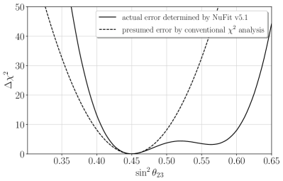
(a)

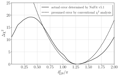
(b)

Figure 2: Comparison of the $\chi^{2}$ profile determined by the global analysis NuFIT v5.1 [72] and the presumed profile computed with eq. (74) in a conventional $\chi^{2}$ analysis for (a) $\sin^{2}\theta_{23}$ and (b) $\delta^{\ell}_{\mathcal{CP}}$.

As a quantitative measurement for the goodness of our fit, we perform a $\chi^{2}$ analysis. We define a $\chi^{2}$ function

$$\chi^{2}(x)~{}=~{}\sum_{i}\Delta\chi^{2}_{i}(x)\;,$$ (73)

where we sum over charged-lepton mass ratios and all observables listed in table 3. For the charged-lepton mass ratios we use

$$\Delta\chi_{i}(x)~{}=~{}\dfrac{\mu_{i,\mathrm{exp}}-\mu_{i,\mathrm{model}}(x)}{\sigma_{i}}\;,$$ (74)

where $\mu_{\mathrm{model}}$ is the prediction of the model and $\mu_{\mathrm{exp}}$ and $\sigma$ are its corresponding experimental best-fit value and the size of its $1\sigma$ error, respectively. For the neutrino-oscillation parameters, we use the profiles of the one dimensional $\Delta\chi^{2}$ projections obtained by the global analysis NuFIT v5.1. This makes a difference especially for $\sin^{2}\theta_{23}$ and $\delta^{\ell}_{\mathcal{CP}}$, as can be directly appreciated from figure 2. For instance, by using a conventional $\Delta\chi^{2}$ obtained from eq. (74), one would underestimate the goodness of the fit by multiple sigma ranges for the second octant of $\theta_{23}$ and also for small values of $\delta^{\ell}_{\mathcal{CP}}$. For $\sin^{2}\theta_{23}<0.45$ the goodness of the fit would be overestimated. We included $\delta^{\ell}_{\mathcal{CP}}$ when calculating $\chi^{2}$ because, even though no values could be excluded with $5\sigma$ by now, experiments do seem to favor some values of $\delta^{\ell}_{\mathcal{CP}}$ over others. We numerically minimize the function $\chi^{2}(x)$ as described in appendix B.

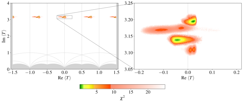
Figure 3: Regions in the fundamental domain of $\Gamma(3)$ that yield fits with $\chi^{2}\leq 25$. Note that a mapping into the fundamental domain of $\mathrm{SL}(2,\mathbbm{Z})$ with a modular transformation $\gamma\in T^{\prime}$ is not possible for this model, since we require the flavon VEVs to be real, i.e. to respect the $\mathcal{CP}$-like symmetry. The analogous flavon VEVs after performing a $T^{\prime}$ transformation would in general be complex. The colors green, yellow, and orange may be interpreted as the $1\sigma$, $2\sigma$, and $3\sigma$ confidence levels, while the opaque red fades out to white until the $5\sigma$ barrier is reached. Note that there are two disconnected $1\sigma$ regions on the right-hand side plot. In the right green region, the best point is $\langle{T}\rangle=0.02279+3.195\,\mathrm{i}$, which yields $\chi^{2}=0.08$. In the left green region, $\langle{T}\rangle=-0.04283+3.139\,\mathrm{i}$ yields $\chi^{2}=0.45$. Therefore, the best-fit value of the model lies in the right green region.

This numerical scan yields a successful fit to current experimental data with an overall $\chi^{2}=0.08$. The regions in moduli space that yield good fits, with $\chi^{2}\leq 25$, are depicted in figure 3. As we see, there are multiple clusters that yield good fits. Interestingly, they have roughly the same shape but are shifted by $T\rightarrow T+\nicefrac{{3}}{{4}}$ while also $\langle{\tilde{\varphi}_{\mathrm{e},1}}\rangle\rightarrow-\langle{\tilde{\varphi}_{\mathrm{e},1}}\rangle$, $\langle{\tilde{\varphi}_{\nu,1}}\rangle\rightarrow-\langle{\tilde{\varphi}_{\nu,1}}\rangle$. Note that this transformation is not part of the eclectic flavor group. It therefore turns out to be an accidental approximate symmetry of the model. This symmetry originates from the properties under modulus shifts of the modular forms of weight 1 that appear in our model. Namely, $T\rightarrow T+\nicefrac{{3}}{{4}}$ results in $\hat{Y}_{1}(T)\rightarrow-\mathrm{i}\,\hat{Y}_{1}(T)$, up to $\mathcal{O}(q)$ corrections, as shown in eq. (13). Moreover, every cluster has two $1\sigma$ (green) regions. As we shall shortly see, this bimodality is inherited by most observables. For the two green regions of the cluster in the fundamental domain of $\mathrm{SL}(2,\mathbbm{Z})$, the best-fit values and $1\sigma$ intervals for the parameters $x$ of the model are listed in table 4. Note that the best-fit values are very close to the predictions from the analytical approximate analysis for the mass ratios given in eqs. (62) and (63).

	right green region		left green region
parameter	best-fit value	$1\sigma$ interval	best-fit value	$1\sigma$ interval
$\operatorname{Re}\,\langle{T}\rangle$	$\phantom{-}0.02279$	$0.01345\rightarrow 0.03087$	$-0.04283$	$-0.05416\rightarrow-0.02926$
$\operatorname{Im}\,\langle{T}\rangle$	$\phantom{-}3.195$	$3.191\rightarrow 3.199$	$\phantom{-}3.139$	$3.135\rightarrow 3.142$
$\langle{\tilde{\varphi}_{\mathrm{e,1}}}\rangle$	$-4.069\cdot 10^{-5}$	$-4.321\cdot 10^{-5}\rightarrow-3.947\cdot 10^{-5}$	$\phantom{-}2.311\cdot 10^{-5}$	$2.196\cdot 10^{-5}\rightarrow 2.414\cdot 10^{-5}$
$\langle{\tilde{\varphi}_{\mathrm{e,2}}}\rangle$	$\phantom{-}0.05833$	$0.05793\rightarrow 0.05876$	$\phantom{-}0.05826$	$0.05792\rightarrow 0.05863$
$\langle{\tilde{\varphi}_{\mathrm{\nu,1}}}\rangle$	$\phantom{-}0.001224$	$0.001201\rightarrow 0.001248$	$-0.001274$	$-0.001304\rightarrow-0.001248$
$\langle{\tilde{\varphi}_{\mathrm{\nu,2}}}\rangle$	$-0.9857$	$-1.0128\rightarrow-0.9408$	$\phantom{-}0.9829$	$0.9433\rightarrow 1.0122$
$\Lambda_{\nu}~{}[\mathrm{eV}]$	$\phantom{-}0.05629$	$0.05442\rightarrow 0.05888$	$\phantom{-}0.05591$	$0.05408\rightarrow 0.05850$
$\,\chi^{2}$	$\phantom{-}0.08$		$\phantom{-}0.45$

Table 4: Best-fit values and their corresponding $1\sigma$ intervals for the two green regions displayed in the plot on the right-hand side of figure 3.

	model			experiment
observable	best fit	$1\sigma$ interval	$3\sigma$ interval	best fit	$1\sigma$ interval	$3\sigma$ interval
$m_{\mathrm{e}}/m_{\mu}$	$0.00473$	$0.00470\rightarrow 0.00477$	$0.00462\rightarrow 0.00485$	$0.00474$	$0.00470\rightarrow 0.00478$	$0.00462\rightarrow 0.00486$
$m_{\mu}/m_{\tau}$	$0.0586$	$0.0581\rightarrow 0.0590$	$0.0572\rightarrow 0.0600$	$0.0586$	$0.0581\rightarrow 0.0590$	$0.0572\rightarrow 0.0600$
$\sin^{2}\theta_{12}$	$0.303$	$0.294\rightarrow 0.315$	$0.275\rightarrow 0.335$	$0.304$	$0.292\rightarrow 0.316$	$0.269\rightarrow 0.343$
$\sin^{2}\theta_{13}$	$0.02254$	$0.02189\rightarrow 0.02304$	$0.02065\rightarrow 0.02424$	$0.02246$	$0.02184\rightarrow 0.02308$	$0.02060\rightarrow 0.02435$
$\sin^{2}\theta_{23}$	$0.449$	$0.436\rightarrow 0.468$	$0.414\rightarrow 0.593$	$0.450$	$0.434\rightarrow 0.469$	$0.408\rightarrow 0.603$
$\delta^{\ell}_{\mathcal{CP}}/\pi$	$1.28$	$1.15\rightarrow 1.47$	$0.81\rightarrow 1.94$	$1.28$	$1.14\rightarrow 1.48$	$0.80\rightarrow 1.94$
$\eta_{1}/\pi\mod 1$	$0.029$	$0.018\rightarrow 0.048$	$-0.031\rightarrow 0.090$	-	-	-
$\eta_{2}/\pi\mod 1$	$0.994$	$0.992\rightarrow 0.998$	$0.935\rightarrow 1.004$	-	-	-
$J_{\mathcal{CP}}$	$-0.026$	$-0.033\rightarrow-0.015$	$-0.035\rightarrow 0.019$	$-0.026$	$-0.033\rightarrow-0.016$	$-0.033\rightarrow 0.000$
$J_{\mathcal{CP}}^{\mathrm{max}}$	$0.0335$	$0.0330\rightarrow 0.0341$	$0.0318\rightarrow 0.0352$	$0.0336$	$0.0329\rightarrow 0.0341$	$0.0317\rightarrow 0.0353$
$\Delta m_{21}^{2}/10^{-5}~{}[\mathrm{eV}^{2}]$	$7.39$	$7.35\rightarrow 7.49$	$7.21\rightarrow 7.65$	$7.42$	$7.22\rightarrow 7.63$	$6.82\rightarrow 8.04$
$\Delta m_{31}^{2}/10^{-3}~{}[\mathrm{eV}^{2}]$	$2.508$	$2.488\rightarrow 2.534$	$2.437\rightarrow 2.587$	$2.521$	$2.483\rightarrow 2.537$	$2.430\rightarrow 2.593$
$m_{1}~{}[\mathrm{eV}]$	$0.0042$	$0.0039\rightarrow 0.0049$	$0.0034\rightarrow 0.0131$	$<0.037$	-	-
$m_{2}~{}[\mathrm{eV}]$	$0.0095$	$0.0095\rightarrow 0.0099$	$0.0092\rightarrow 0.0157$	-	-	-
$m_{3}~{}[\mathrm{eV}]$	$0.0504$	$0.0501\rightarrow 0.0505$	$0.0496\rightarrow 0.0519$	-	-	-
$\sum_{i}m_{i}~{}[\mathrm{eV}]$	$0.0641$	$0.0636\rightarrow 0.0652$	$0.0628\rightarrow 0.0806$	$<0.120$	-	-
$m_{\beta\beta}~{}[\mathrm{eV}]$	$0.0055$	$0.0045\rightarrow 0.0064$	$0.0040\rightarrow 0.0145$	$<0.036$	-	-
$m_{\beta}~{}[\mathrm{eV}]$	$0.0099$	$0.0097\rightarrow 0.0102$	$0.0094\rightarrow 0.0159$	$<0.8$	-	-
$\chi^{2}$	$0.08$

Table 5: Comparison of the best-fit values in the lepton sector of our model against the experimental data. In the columns 2–4 we present the best values from our fit with their $1\sigma$ and $3\sigma$-error intervals. We have added $\mod 1$ for $\eta_{1,2}$ because there are two disconnected $1\sigma$ regions shifted by $\pi$, cf. figure 6. In the last three columns, we include the experimental best fit and $1\sigma$ ranges for the charged-lepton mass ratios at the GUT scale, assuming $\tan\beta=10$, $M_{\mathrm{SUSY}}=10$ TeV, and $\bar{\eta}_{b}=0.09375$, taken from [71]. In addition, we give the best-fit values and error intervals for the neutrino-oscillation parameters as obtained by the global analysis NuFIT v5.1 [72] with Super-Kamiokande data for normal ordering.

In table 5, we summarize the best-fit values for the observables resulting from our numerical scan. At the best-fit point, all observables (i.e. the charged lepton mass ratios, the neutrino mass-squared differences, and the four lepton mixing matrix parameters) are within the $1\sigma$ interval of the current experimental data. In addition, even though we did not demand it in our fit, it turns out that the results of the fit are in agreement with the experimental bounds for the lightest neutrino mass $m_{1}$, the sum of neutrino masses $\sum_{i}m_{i}$, the effective mass for neutrino-less double beta decay $m_{\beta\beta}$, and the neutrino mass observable in ${}^{3}\mathrm{H}$ beta decay $m_{\beta}$, cf. [75], [76], [77], and [78], respectively.

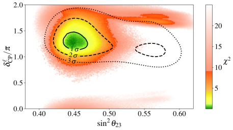
Figure 4: Fitted regions with $\chi^{2}\leq 25$ in the space of $\sin^{2}\theta_{23}$ and $\delta^{\ell}_{\mathcal{CP}}$ achieved in our model. The black lines delimit the experimental $1$, $2$, and $3\sigma$ regions as determined by the global analysis NuFIT. The bimodality appearing in moduli space, cf. figure 3, seems to be absent in the $\theta_{23}-\delta^{\ell}_{\mathcal{CP}}$ plane, as the two green regions overlap and therefore appear as only one green region here.

For observables whose values have not yet been determined by experiment, our model has the following predictions:

• As shown in figure 4, in our model $\theta_{23}$ is preferably found in the first octant, i.e. $\theta_{23}<45^{\circ}$. Taking the atmospheric data provided by Super-Kamiokande into account, this octant is currently also preferred by experiment in the case of normal ordering. Unfortunately, for this octant, the model does not provide a prediction for the $\mathcal{CP}$ violating phase $\delta_{\mathrm{\mathcal{CP}}}^{\ell}$.

• The model has a rather precise prediction for the neutrino masses, especially for the heaviest neutrino mass, cf. figure 5. At $1\sigma$, the neutrino masses are predicted to be $3.9~{}\mathrm{meV}<m_{1}<4.9~{}\mathrm{meV}$, $9.5~{}\mathrm{meV}<m_{2}<9.9~{}\mathrm{meV}$, and $50.1~{}\mathrm{meV}<m_{3}<50.5~{}\mathrm{meV}$.

• Only Majorana phases that are close to $\mathcal{CP}$-conserving values are compatible with the fit of our model. For more details, see figure 6.

• The prediction for the effective neutrino mass $m_{\beta\beta}$ is, unfortunately, not reachable by the next-generation experiments for neutrinoless double beta decay. However, potential next-to-next generation experiments, e.g. CUPID-1T [79], aim at covering the predicted region, see figure 7.

• We have performed a wide numerical scan and did not find any successful fit that accepts inverted ordered neutrino masses. Hence, we observe that our model clearly prefers normal ordering.

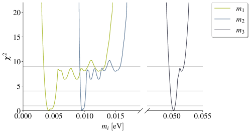
Figure 5: Projections of $\chi^{2}$ on the neutrino masses, which are clearly normal ordered.

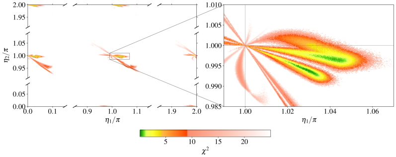
Figure 6: Majorana phases predicted by our model. Note that the Majorana phases are found to be in general near $\mathcal{CP}$-conserving values. The appearance of two $1\sigma$ (green) regions in this plot stems from the bimodality found in moduli space: each green region in the plot on the right-hand side arises from a different $1\sigma$ region of the fundamental domain of $\mathrm{SL}(2,\mathbbm{Z})$ in figure 3.

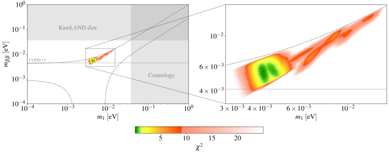
Figure 7: Effective neutrino mass for $0\nu\beta\beta$ as a function of the lightest neutrino mass. The dashed lines delimit the experimentally admissible region within $3\sigma$ for normal ordering. Gray-shaded areas are excluded by KamLAND-Zen [77] or cosmological bounds [75, 76]. The $1\sigma$ and $2\sigma$ (green and yellow) regions are within the bounds that next-to-next generation experiments are aiming at. For example, the stated preliminary exclusion sensitivity of the CUPID-1T experiment goes down to $4.1~{}\mathrm{meV}$ [79], which is indicated in the plot by a thin gray line. As for Majorana phases, cf. figure 6, the appearance of two $1\sigma$ (green) regions in this plot is related to the bimodality in moduli space, cf. figure 3.

5 Simultaneous fit of quark and lepton sectors

So far, we have discussed only the lepton sector. It has been fitted by choosing appropriate VEVs for the modulus $T$ and the flavon triplets $\varphi_{\mathrm{e}}$ and $\varphi_{\nu}$. Let us now include in our analysis the masses and mixings of quarks. Inspecting the superpotential (15), we realize that up-type quark Yukawa couplings include an additional flavon triplet $\varphi_{\mathrm{u}}$ while down-type Yukawas share the flavon triplet $\varphi_{\mathrm{e}}$. Consequently, at leading order i) the structure of the mass matrices of up and down-type quarks are equal, and ii) the masses of charged leptons and down-type quarks differ only by their overall scale. The latter contradicts experimental observations, but it can be amended by taking into account contributions from the Kähler potential. As discussed in section 2.5, if flavons develop VEVs, there can be considerable off-diagonal corrections to the Kähler metric already at next-to-leading order.

In principle, Kähler corrections can affect both leptons and quarks. However, for simplicity, we assume that the parameters in the lepton sector yield negligible contributions to additional terms in the Kähler potential. That is, only the quark sector will be influenced by Kähler corrections. According to our previous discussion in section 2.5, the next-to-leading order corrections to the Kähler metric of quark fields $\Psi\in\{\bar{u},\bar{d},q\}$ take the form (see eq. (44))

$$K_{ij}^{f}\supset\lambda_{\varphi_{\mathrm{eff}}}^{f}\,\left(A_{ij}^{f}+\kappa_{\varphi_{\mathrm{eff}}}^{f}\,B_{ij}^{f}\right)\;,$$ (75)

where $f\in\{\mathrm{u,d,q}\}$ labels the effective flavons and Kähler parameters associated with each quark field, explicitly defined in eqs. (44)–(49). To simplify our notation, we have suppressed the arguments of the Kähler matrix elements, such that

$$A_{ij}^{f}:=A_{ij}(\tilde{\varphi}_{\mathrm{eff}}^{(A),f})\qquad\text{and}\qquad B_{ij}^{f}:=B_{ij}(\tilde{\varphi}_{\mathrm{eff}}^{(B),f})\;.$$ (76)

These matrix elements are quadratic in the VEVs of the components of the effective flavon triplets. However, since these VEVs appear in the Kähler metric always accompanied by the coefficients $\lambda_{\varphi_{\mathrm{eff}}}^{f}$, it is convenient to use instead the parameters

$$\alpha_{i}^{f}:=\sqrt{\lambda_{\varphi_{\mathrm{eff}}}^{f}}\,\langle{\tilde{\varphi}_{\mathrm{eff},i}^{(A),f}}\rangle\qquad\text{and}\qquad\beta_{i}^{f}:=\sqrt{\lambda_{\varphi_{\mathrm{eff}}}^{f}}\,\langle{\tilde{\varphi}_{\mathrm{eff},i}^{(B),f}}\rangle\;,$$ (77)

such that

$$\lambda_{\varphi_{\mathrm{eff}}}^{f}A_{ij}^{f}=\alpha_{i}^{f}\,\alpha_{j}^{f}\;,$$ (78)

and $\lambda_{\varphi_{\mathrm{eff}}}^{f}B_{ij}^{f}$ is quadratic in $\beta^{f}$ up to $\mathcal{O}(1)$ factors. Note that the parameters $\alpha_{i}^{f}$ and $\beta_{i}^{f}$ represent a good measure of the size of the Kähler corrections.

parameter		best-fit value
	$\operatorname{Im}\,\langle{T}\rangle$	$\phantom{-}3.195$
	$\operatorname{Re}\,\langle{T}\rangle$	$\phantom{-}0.02279$
	$\langle{\tilde{\varphi}_{\mathrm{u},1}}\rangle$	$\phantom{-}2.0332\cdot 10^{-4}$
	$\langle{\vartheta_{\mathrm{u},1}}\rangle$	$\phantom{-}1.6481$
	$\langle{\tilde{\varphi}_{\mathrm{u},2}}\rangle$	$\phantom{-}6.3011\cdot 10^{-2}$
	$\langle{\vartheta_{\mathrm{u},2}}\rangle$	$-1.5983$
	$\langle{\tilde{\varphi}_{\mathrm{e},1}}\rangle$	$-4.069\cdot 10^{-5}$
	$\langle{\tilde{\varphi}_{\mathrm{e},2}}\rangle$	$\phantom{-}5.833\cdot 10^{-2}$
	$\langle{\tilde{\varphi}_{\nu,1}}\rangle$	$\phantom{-}1.224\cdot 10^{-3}$
	$\langle{\tilde{\varphi}_{\nu,2}}\rangle$	$-0.9857$
superpotential	$\Lambda_{\nu}~{}[\mathrm{eV}]$	$\phantom{-}0.05629$
	$\alpha_{1}^{\mathrm{u}}$	$-0.94917$
	$\alpha_{2}^{\mathrm{u}}$	$\phantom{-}0.0016906$
	$\alpha_{3}^{\mathrm{u}}$	$\phantom{-}0.31472$
	$\alpha_{1}^{\mathrm{d}}$	$\phantom{-}0.95067$
	$\alpha_{2}^{\mathrm{d}}$	$\phantom{-}0.0077533$
	$\alpha_{3}^{\mathrm{d}}$	$\phantom{-}0.30283$
	$\alpha_{1}^{\mathrm{q}}$	$-0.96952$
	$\alpha_{2}^{\mathrm{q}}$	$-0.20501$
Kähler potential	$\alpha_{3}^{\mathrm{q}}$	$\phantom{-}0.041643$

(a) (a)

observable		model best fit	exp. best fit	exp. $1\sigma$ interval
	$m_{\mathrm{u}}/m_{\mathrm{c}}$	$\phantom{-}0.00193$	$\phantom{-}0.00193$	$0.00133\rightarrow 0.00253$
	$m_{\mathrm{c}}/m_{\mathrm{t}}$	$\phantom{-}0.00280$	$\phantom{-}0.00282$	$0.00270\rightarrow 0.00294$
	$m_{\mathrm{d}}/m_{\mathrm{s}}$	$\phantom{-}0.0505$	$\phantom{-}0.0505$	$0.0443\rightarrow 0.0567$
	$m_{\mathrm{s}}/m_{\mathrm{b}}$	$\phantom{-}0.0182$	$\phantom{-}0.0182$	$0.0172\rightarrow 0.0192$
	$\vartheta_{12}~{}[\mathrm{deg}]$	$\,\;\!13.03$	$\,\;\!13.03$	$12.98\rightarrow 13.07$
	$\vartheta_{13}~{}[\mathrm{deg}]$	$\phantom{-}0.200$	$\phantom{-}0.200$	$0.193\rightarrow 0.207$
	$\vartheta_{23}~{}[\mathrm{deg}]$	$\phantom{-}2.30$	$\phantom{-}2.30$	$2.26\rightarrow 2.34$
quark sector	$\delta_{\mathcal{CP}}^{\mathrm{q}}~{}[\mathrm{deg}]$	$\,\;\!69.2$	$\,\;\!69.2$	$66.1\rightarrow 72.3$
	$m_{\mathrm{e}}/m_{\mu}$	$\phantom{-}0.00473$	$\phantom{-}0.00474$	$0.00470\rightarrow 0.00478$
	$m_{\mu}/m_{\tau}$	$\phantom{-}0.0586$	$\phantom{-}0.0586$	$0.0581\rightarrow 0.0590$
	$\sin^{2}\theta_{12}$	$\phantom{-}0.303$	$\phantom{-}0.304$	$0.292\rightarrow 0.316$
	$\sin^{2}\theta_{13}$	$\phantom{-}0.0225$	$\phantom{-}0.0225$	$0.0218\rightarrow 0.0231$
	$\sin^{2}\theta_{23}$	$\phantom{-}0.449$	$\phantom{-}0.450$	$0.434\rightarrow 0.469$
	$\delta_{\mathcal{CP}}^{\ell}/\pi$	$\phantom{-}1.28$	$\phantom{-}1.28$	$1.14\rightarrow 1.48$
	$\eta_{1}/\pi$	$\phantom{-}0.029$	-	-
	$\eta_{2}/\pi$	$\phantom{-}0.994$	-	-
	$J_{\mathcal{CP}}$	$-0.026$	$-0.026$	$-0.033\rightarrow-0.016$
	$J_{\mathcal{CP}}^{\mathrm{max}}$	$\phantom{-}0.0335$	$\phantom{-}0.0336$	$0.0329\rightarrow 0.0341$
	$\Delta m_{21}^{2}/10^{-5}~{}[\mathrm{eV}^{2}]$	$\phantom{-}7.39$	$\phantom{-}7.42$	$7.22\rightarrow 7.63$
	$\Delta m_{31}^{2}/10^{-3}~{}[\mathrm{eV}^{2}]$	$\phantom{-}2.521$	$\phantom{-}2.510$	$2.483\rightarrow 2.537$
	$m_{1}~{}[\mathrm{eV}]$	$\phantom{-}0.0042$	$\!<\!0.037$	-
	$m_{2}~{}[\mathrm{eV}]$	$\phantom{-}0.0095$	-	-
	$m_{3}~{}[\mathrm{eV}]$	$\phantom{-}0.0504$	-	-
	$\sum_{i}m_{i}~{}[\mathrm{eV}]$	$\phantom{-}0.0641$	$\!<\!0.120$	-
	$m_{\beta\beta}~{}[\mathrm{eV}]$	$\phantom{-}0.0055$	$\!<\!0.036$	-
lepton sector	$m_{\beta}~{}[\mathrm{eV}]$	$\phantom{-}0.0099$	$\!<\!0.8$	-
	$\chi^{2}$	$\phantom{-}0.11$

(b) (b)

Table 6: Results of a simultaneous fit of the quark and lepton sectors with $\chi^{2}=0.11$. (a) Values of the model parameters at the best-fit point. The parameter values in the lepton sector coincide with the modulus and flavon VEVs showed in table 4. In addition, for the quark sector we provide the (complex) components of the flavon VEV $\langle{\tilde{\varphi}_{\mathrm{u}}}\rangle$ appearing in the superpotential, along with the effective Kähler parameters $\alpha_{i}^{f}$, $f\in\{\mathrm{u,d,q}\}$ and $i\in\{1,2,3\}$, defined in eq. (77). (b) Best-fit values of flavor observables obtained from our model. We compare them with the corresponding experimental best-fit value; we include the experimental $1\sigma$ error. The quark-sector observables are successfully fitted while keeping untouched the lepton-sector fit presented in table 5.

The additional parameters of the quark sector include first the complex components of the normalized up-type flavon triplet

$$\langle{\tilde{\varphi}_{\mathrm{u}}}\rangle~{}=~{}\Big{(}\langle{\tilde{\varphi}_{\mathrm{u},1}}\rangle\,\exp\;\!\!\left(\mathrm{i}\langle{\vartheta_{\mathrm{u},1}}\rangle\right),\langle{\tilde{\varphi}_{\mathrm{u},2}}\rangle\,\exp\;\!\!\left(\mathrm{i}\langle{\vartheta_{\mathrm{u},2}}\rangle\right),1\Big{)}\;.$$ (79)

Furthermore, the Kähler corrections introduce 9 parameters $\alpha_{i}^{f}$, 9 $\beta_{i}^{f}$ and 3 $\kappa_{\varphi_{\mathrm{eff}}}^{f}$. In order to simplify somewhat our fit, we impose the following constraints:

• $\kappa_{\varphi_{\mathrm{eff}}}^{f}=1$ for all $f\in\{\mathrm{u,d,q}\}$,

• $\alpha_{i}^{f}=\beta_{i}^{f}$ for all $f$ and $i\in\{1,2,3\}$, and

• all $\alpha_{i}^{f}$ are real.

While these constraints may appear ad-hoc, we stress that the philosophy here is not to scan the full parameter space but to demonstrate, in the first place, that there is a region in the parameter space that indeed agrees with a realistic low energy phenomenology. Taking the constraints into account, we arrive at a remaining set of 13 quark parameters that we include in our numerical scan, aiming at a global fit of both leptons and quarks. The numerical procedure to achieve the global fit is based on a $\chi^{2}$ minimization, analogous to the one used in the lepton sector, which is discussed in detail in appendix B. As for charged leptons, the experimental data we consider for quarks are the mass ratios and mixing parameters at the GUT scale [71], assuming a running with $\tan\beta=10$, $M_{\mathrm{SUSY}}=10$ TeV, and $\bar{\eta}_{b}=0.09375$, as in refs. [33, 73]. These experimental best-fit values together with their respective errors are presented in the last two columns of table 6b.

The resulting best-fit values are displayed in table 6. The modulus and flavon VEVs of the model have the values shown in table 6a. We point out that the magnitude of the Kähler corrections needed to arrive at a successful global fit all satisfy $\alpha^{f}_{i}<1$. Also, the VEVs of the modulus $\langle{T}\rangle$ and the lepton flavons $\langle{\tilde{\varphi}_{\mathrm{e},i}}\rangle$ and $\langle{\tilde{\varphi}_{\nu,i}}\rangle$ preserve the values obtained in the lepton fit, cf. table 5. In table 6b we compare our best fit against the experimental values of quark and lepton observables. Our global fit of all fermion mass ratios, mixing angles and $\mathcal{CP}$ phases exhibits $\chi^{2}=0.11$. Although we do not provide any prediction in the quark sector, it is remarkable that the eclectic scenario arising from a string compactification can fit the observed data so well.

Before concluding, let us mention some caveats of our model. First, the VEV parameters of the model included in eqs. (72) and (79) as well as the Kähler parameters of eqs. (77) have been considered here to be free. However, in a full string model the computation of the couplings and the dynamic stabilization of the VEVs are in principle achievable. Unfortunately, these tasks have not been solved so far, remaining as open questions for our model. Secondly, notice that the values of the Kähler parameters in our fit, displayed in table 6a, are all controllable in the sense that they arise in a Kähler potential that is explicitly constrained by the eclectic flavor group and, moreover, their magnitudes turn out to be smaller than unity ensuring the perturbativity of our model. Yet, because of its complexity, the rigorous string computation of these parameters lies still beyond the scope of our study. Finally, our focus is the flavor puzzle only, assuming that all other phenomenological questions of particle physics and cosmology can be solved by some methods introduced in many earlier influential works. For example, we have assumed that all exotic matter states appearing in table 2 can acquire masses much larger than the physical scale of the flavor sector in supersymmetric vacua [80, 60, 81, 82]. One might then argue that only the physical right-handed neutrinos and Higgs doublets are left massless as a result of the existence of some unbroken ($R$-)symmetries either beyond the flavor sector [83, 84, 85] or intimately linked with it [86]. As shown in those works, such symmetries could also be relevant for proton stability and the suppression of the $\mu$-term. In addition, relaxing our assumption on the decoupling of the extra right-handed neutrinos in table 2 might be instrumental to arrive at a better understanding of the relation between the Majorana and the observable neutrino mass scales [87]. Our scheme also admits proposals to solve the discrepancy between the GUT and string scale in heterotic models [88, 89] since it can be embedded in anisotropic compactifications. Furthermore, heterotic orbifolds seem to be equipped with useful properties to achieve supersymmetry breakdown [90]. All these aspects should be studied elsewhere in detail to complete our construction and extend it to other relevant phenomenological questions, such as identifying the cause of inflation, the origin of dark matter and the baryon asymmetry of the Universe.

6 Conclusions and Outlook

We have studied the flavor phenomenology of the lepton and quark sectors emerging from a specific $\mathbbm{T}^{6}/\mathbbm{Z}_{3}\times\mathbbm{Z}_{3}$ heterotic orbifold model that gives rise to the eclectic flavor group $\Omega(2)$. This TD scenario combines the virtues of a modular $T^{\prime}$ and a traditional $\Delta(54)$ flavor symmetry, while avoiding the arbitrariness in the choice of quantum numbers of matter fields inherent to BU constructions. The (traditional, modular and gauge symmetry) representations of matter fields as well as their modular weights are entirely fixed by the compactification. In our example model, SM fermions and flavons form identical flavor triplets and exhibit equal (fractional) modular weights, cf. table 1. Hence, the structure of the superpotential and Kähler potential are determined by the theory, guaranteeing, in particular, a canonical leading-order Kähler potential, as is most frequently assumed in the BU approach. However, in addition, our setup also allows us to control non-canonical, higher-order, Planck-suppressed corrections to the Kähler potential that arise after the traditional flavor symmetry is spontaneously broken by flavons. We computed these corrections (to next-to-leading order), which turn out to be instrumental for a successful phenomenological fit since they contribute to the structure of mass matrices. Both, the modulus and some of the flavons inherent to the construction must attain non-trivial VEVs in order to break the modular and traditional components of the eclectic symmetry, as required by phenomenology. Special values of these VEVs lead to discrete remnants of the flavor group that can appear as approximate discrete symmetries at low energies [7].

In our string-derived example model, we have explicitly computed the leading-order superpotential (15) and confirmed the canonical leading-order structure of the Kähler potential (39). These results reveal that our model accommodates naturally a type-I see-saw mechanism as explanation for the neutrino masses. We have shown that points in moduli space perturbatively close to the symmetry-enhanced point $\langle{T}\rangle=\mathrm{i}\infty$ enjoy various approximate symmetries as remnants of the eclectic group. Their successive spontaneous breaking through the misaligned VEVs of the modulus and flavon fields can account for technically natural (symmetry-protected) correct hierarchies. The tight, symmetry-based constraints allow us to derive approximate analytical expressions for the mass hierarchies, as explained in section 3.

In order to fully explore the phenomenology of the model, we have performed a numerical analysis of the charged-lepton and neutrino sectors. We found that the 11 independent observables listed in table 5 can be well fitted by adjusting seven free parameters corresponding to the VEVs of the modulus and flavons as well as the neutrino mass scale. Their values at the best-fit point are presented in table 4 and show that our analytical treatment is fairly accurate. The octant of $\theta_{23}$, the normal ordering of neutrino masses, the observable values of $m_{\beta\beta}$, as well as the neutrino Majorana phases are predictions of the fit. These results are illustrated in figures 4–7.

Next-to-leading-order Kähler corrections turn out to be crucial to arrive at a model of flavor that includes the quark sector in a phenomenologically viable manner. This is another consequence of the highly constrained nature of TD constructions, as our example model contains only a single non-singlet flavon field that is responsible for the structure and hierarchies of down-quark and charged-lepton Yukawa couplings, as well as of the neutrino Majorana mass term. This results in a particular kind of bottom-tau unification that must be modified in order to arrive at a realistic phenomenology. We have shown that this can be achieved thanks to the presence of next-to-leading-order Kähler corrections, which allowed us to obtain a successful numerical fit to quark phenomenology that does not change our predictions for the lepton sector.

In summary, we have presented for the first time a UV-complete, full string theory model that exhibits a flavor scheme that can accomodate the experimentally observed pattern of quark and lepton flavor phenomenology. Reducing the number of free parameters was possible by taking into account the restrictive constraints on the effective superpotential and Kähler potential arising from the entire, partly non-linearly realized, eclectic flavor symmetry. Achieving the ambitious goal of a complete fit to the low-energy flavor data was possible only as a consequence of the existence of controllable Kähler corrections.

This represents the first decisive step towards connecting the BU and TD efforts in the quest for an ultimate theory of flavor, and demonstrates the potential of this TD approach. It would be interesting to compare our results to the outcome of similar TD constructions, such as the orbifold models of type B–D classified in ref. [7], orbifold constructions endowed with a $\mathbbm{T}^{2}/\mathbbm{Z}_{2}$ sector [48, 49], or other TD scenarios that can admit three fermion generations and metaplectic flavor symmetries [42], and also exhibit eclectic features [40]. Moreover, quasi–eclectic models [91] offer another interesting possibility to explore in order to further connect the BU and TD approaches.

Future efforts should aim at further reducing the number of free parameters, either by rigorous string computations of some of the low energy parameters, or by identifying other potentially realistic string setups that are even more constrained by symmetry. Further attention should also be paid to the field-theoretical minimization of the flavon potential as well as to the longstanding question of modulus stabilization.

Appendix A Kähler potential at next-to-leading order

In order to arrive at the next-to-leading order Kähler potential, eq. (44), one must compute the tensor products of the relevant representations (by using e.g. ref. [92]). Here we discuss in detail the results of the computation.

The first tensor product in eq. (42) is given by

$$T_{1,a}~{}=~{}\left[\varphi^{*}\otimes\varphi\otimes\Psi^{*}\otimes\Psi\right]_{\boldsymbol{1},a}\;.$$ (80)

This product has two invariant singlet contractions, i.e. $a\in\{1,2\}$. For $a=1$ it reads

$$T_{1,a=1}~{}=~{}\Psi^{\dagger}\begin{pmatrix}|\varphi_{1}|^{2}&\varphi_{1}\,\varphi_{2}^{*}&\varphi_{1}\,\varphi_{3}^{*}\\ \varphi_{2}\,\varphi_{1}^{*}&|\varphi_{2}|^{2}&\varphi_{2}\,\varphi_{3}^{*}\\ \varphi_{3}\,\varphi_{1}^{*}&\varphi_{3}\,\varphi_{2}^{*}&|\varphi_{3}|^{2}\end{pmatrix}\Psi\;.$$ (81)

Here $\varphi_{i}$ corresponds to the $i$-th component of the flavor triplet $\varphi$, or equivalently

$$T_{1,a=1}~{}=~{}\Psi^{*}_{i}~{}A_{ij}(\varphi)~{}\Psi_{j}\;,$$ (82)

where the components of the matrix $A$ are given by

$$A_{ij}(\varphi)~{}:=~{}\varphi_{i}\,\varphi_{j}^{*}\;,$$ (83)

and summation over repeated indices is implied. The second invariant singlet contraction, i.e. $T_{1,a=2}=\Psi^{*}_{j}~{}\varphi_{i}\,\varphi^{*}_{i}~{}\Psi_{j}$, is irrelevant because it is proportional to the identity matrix and hence its contribution to the Kähler metric can be absorbed by the symmetry-invariant constant $\chi$ of the leading-order Kähler potential (40). Thus, we shall not discuss it here.

The second tensor product in the next-to-leading order Kähler potential is given by

$$T_{2,a}~{}=~{}\left[\left(\hat{Y}^{(1)}(T)\right)^{*}\otimes\hat{Y}^{(1)}(T)\otimes\varphi^{*}\otimes\varphi\otimes\Psi^{*}\otimes\Psi\right]_{\boldsymbol{1},a}\;,\qquad a\in\{1,2,3\}\;.$$ (84)

This tensor product yields three linearly-independent invariant terms, but only two of them cannot be absorbed in (40). The first nontrivial term reads

$$T_{2,a=1}~{}=~{}\Psi^{*}_{i}~{}|\hat{Y}^{(1)}(T)|^{2}\,A_{ij}(\varphi)~{}\Psi_{j}\;.$$ (85)

Note that this term, apart from the overall factor of $|\hat{Y}^{(1)}(T)|^{2}$, structurally yields the same Kähler metric as the first tensor product (82). The second invariant singlet contraction reads

$$T_{2,a=2}~{}=~{}\Psi^{*}_{i}~{}\left(B_{ij}(\varphi)+|\hat{Y}_{2}|^{2}|\varphi|^{2}\delta_{ij}\right)\Psi_{j}\;,$$ (86)

where

$$B_{ij}(\varphi)~{}=~{}\begin{cases}\left(|\hat{Y}_{1}|^{2}-2\,|\hat{Y}_{2}|^{2}\right)\,\varphi_{i}\,\varphi_{j}^{*}\;,&\text{for\ }i=j\\ -|\hat{Y}_{1}|^{2}\,\varphi_{i}\,\varphi_{j}^{*}+\sqrt{2}\left(\hat{Y}_{1}\,\hat{Y}_{2}^{*}\,\varphi_{i}^{*}\,\varphi_{k}+\hat{Y}_{2}\,\hat{Y}_{1}^{*}\,\varphi_{k}^{*}\,\varphi_{j}\right)\;,&\text{for\ }k\neq i\neq j\neq k\;.\end{cases}$$ (87)

As before, the term proportional to $\delta_{ij}$ in (86) can be absorbed in (40) and will thus be ignored.

Using eqs. (82) and (86), we find that the next-to-leading order contributions to the Kähler metric (42) that are not proportional to $\delta_{ij}$, are given by

$$K_{ij}^{(\mathrm{non-id})}~{}\supset ~{}\sum_{\varphi}\left[\left(\left(-\mathrm{i}T+\mathrm{i}\bar{T}\right)^{\nicefrac{{-4}}{{3}}}\,\zeta_{1}^{(\varphi)}+\left(-\mathrm{i}T+\mathrm{i}\bar{T}\right)^{\nicefrac{{-1}}{{3}}}\,\zeta_{1}^{(Y\varphi)}|\hat{Y}^{(1)}(T)|^{2}\right)\,A_{ij}(\varphi)\right.$$ (88)

$$\qquad~{}+\left.\left(-\mathrm{i}T+\mathrm{i}\bar{T}\right)^{\nicefrac{{-1}}{{3}}}\,\zeta_{2}^{(Y\varphi)}~{}B_{ij}(\varphi)\right]\;,$$

where we sum over all flavon triplets $\varphi$ (with all possible modular weights) that develop VEVs. We stress that the noncanonical contributions (88) arise only as a result of the breaking of the traditional flavor symmetry by flavon VEVs, and that they are clearly Planck suppressed.

Appendix B Numerical procedure

Let us describe here in detail the numerical procedure we follow to arrive at the fit of the lepton sector. The goal of the numerical procedure is to explore the parameter space of the model parameters $x$ defined in eq. (72) in order to find the regions that yield values of lepton masses and mixings that are in agreement with experimental observations. In detail, we search for parameters that yield $\chi^{2}\leq 25$ corresponding to a compatibility with $5\sigma$. Moreover, we also want to identify the point in parameter space that yields the best match to the experimental data. We therefore split the numerical analysis in two steps: i) First, we find all minima with $\chi^{2}\leq 25$; and ii) then we explore the regions around these minima.

The first step is a typical optimization problem that can be conveniently approached by using the non-linear optimization interface lmfit [93]. We start by picking a random start-point in the parameter space, whose boundaries we set to

$$0~{}<~{}\left|\langle{\tilde{\varphi}_{\mathrm{e},1}}\rangle\right|,~{}\left|\langle{\tilde{\varphi}_{\mathrm{e},2}}\rangle\right|~{}<~{}1\;, \quad 0~{}<~{}\left|\langle{\tilde{\varphi}_{\nu,1}}\rangle\right|,~{}\left|\langle{\tilde{\varphi}_{\nu,2}}\rangle\right|~{}<~{}2\;,$$ (89a)

$$0~{}<~{}\left|\operatorname{Re}\,\langle{T}\rangle\right|~{}<~{}1.5\;, \quad 0~{}<~{}\operatorname{Im}\,\langle{T}\rangle~{}<~{}5\;.$$ (89b)

As we expect the flavon VEVs to be hierarchically ordered, we sample them with a blend of a uniform and a logarithmic distribution. Moreover, we use the analytical result $|\langle{\tilde{\varphi}_{\mathrm{e,2}}}\rangle|~{}\approx~{}\frac{m_{\mu}}{m_{\tau}}~{}=~{}0.0586$ obtained in section 3.2.1 and sample $|\langle{\tilde{\varphi}_{\mathrm{e,2}}}\rangle|$ only in the vicinity of this value. To the chosen start-point, we then consecutively apply five randomly chosen minimization algorithms included in the lmfit interface. For our setup, especially the algorithms ‘Constrained trust-region’ and ‘L-BFGS-B’ deliver good results. We repeat this procedure until roughly 1000 points with $\chi^{2}\leq 25$ and no new minima are found by the algorithms.

Finally, we explore the neighborhood of each minimum using the Markov Chain Monte Carlo (MCMC) sampler emcee [94], which is also supported by lmfit. The MCMC sampler chooses random points with a probability function that it tries to couple to $\chi^{2}$. They are therefore well suited to provide information on the vicinity of the minima and hence the boundaries of the respective confidence levels.

Although similar methods have been thoroughly explained in other works, see e.g. [95], we make our python code available upon request to be applied both in BU and TD constructions. Please, send your inquiries preferably to alexander.baur@tum.de.

Appendix C Complete spectrum of a model with $\Omega(2)$ eclectic flavor symmetry

We provide all quantum numbers of the massless spectrum of our example $\mathbbm{T}^{6}/\mathbbm{Z}_{3}\times\mathbbm{Z}_{3}$ heterotic orbifold model, including the representations under $G_{SM}=\mathrm{SU}(3)_{c}\times\mathrm{SU}(2)_{L}\times\mathrm{U}(1)_{Y}$, the eclectic flavor group $\Omega(2)=\Delta(54)\cup T^{\prime}\cup\mathbbm{Z}_{9}^{R}$ (along with the associated modular weights $n$), and the extra $\mathbbm{Z}_{3}{}^{3}$ flavor and ‘hidden’ $\mathrm{SU}(4)\times\mathrm{U}(1)_{\textrm{anom}}\times\mathrm{U}(1)^{8}$ gauge factors.

		Flavor charges							‘Hidden’ gauge charges
sector	$G_{SM}^{\phantom{A^{A}}}$	$\Delta(54)$	$T^{\prime}$	$\mathbbm{Z}_{9}^{R}$	$n$	$\mathbbm{Z}_{3}$	$\mathbbm{Z}_{3}$	$\mathbbm{Z}_{3}$	$\mathrm{SU}(4)$	$q_{\text{anom}}$	$q_{2}$	$q_{3}$	$q_{4}$	$q_{5}$	$q_{6}$	$q_{7}$	$q_{8}$	$q_{9}$	labels
$U_{1}^{\phantom{A^{A^{A}}}}$	$(\boldsymbol{1},\boldsymbol{2})_{\frac{1}{2}}$	$\boldsymbol{1}$	$\boldsymbol{1}$	$0$	$0$	$1$	$1$	$1$	$\boldsymbol{1}$	$0$	$1$	$0$	$0$	$0$	$0$	$-59$	$32$	$-124$	$H_{u}$
	$(\boldsymbol{1},\boldsymbol{2})_{-\frac{1}{2}}$	$\boldsymbol{1}$	$\boldsymbol{1}$	$0$	$0$	$1$	$1$	$1$	$\boldsymbol{1}$	$0$	$1$	$0$	$0$	$0$	$0$	$59$	$-32$	$124$	$H_{d}$
	$(\boldsymbol{1},\boldsymbol{1})_{0}$	$\boldsymbol{1}$	$\boldsymbol{1}$	$0$	$0$	$1$	$1$	$1$	$\boldsymbol{1}$	$0$	$-2$	$0$	$0$	$0$	$0$	$0$	$0$	$0$	$\phi^{0}$
	$(\boldsymbol{3},\boldsymbol{1})_{\frac{2}{3}}$	$\boldsymbol{1}$	$\boldsymbol{1}$	$0$	$0$	$1$	$1$	$1$	$\boldsymbol{1}$	$0$	$0$	$0$	$0$	$0$	$-73$	$-90$	$-24$	$93$	$U_{1}$
$U_{2}^{\phantom{A^{A}}}$	$(\boldsymbol{1},\boldsymbol{1})_{0}$	$\boldsymbol{1}$	$\boldsymbol{1}$	$0$	$0$	$1$	$1$	$1$	$\boldsymbol{1}$	$-2$	$-1$	$0$	$0$	$0$	$73$	$149$	$-8$	$-125$	$\phi^{0}_{\mathrm{M}}$
	$(\boldsymbol{1},\boldsymbol{1})_{0}$	$\boldsymbol{1}$	$\boldsymbol{1}$	$0$	$0$	$1$	$1$	$1$	$\boldsymbol{1}$	$-2$	$0$	$2$	$-38$	$32$	$42$	$-84$	$264$	$30$	$s_{1}$
	$(\boldsymbol{1},\boldsymbol{1})_{0}$	$\boldsymbol{1}$	$\boldsymbol{1}$	$0$	$0$	$1$	$1$	$1$	$\boldsymbol{1}$	$0$	$0$	$-7$	$16$	$-73$	$0$	$0$	$0$	$0$	$s_{2}$
	$(\boldsymbol{1},\boldsymbol{1})_{0}$	$\boldsymbol{1}$	$\boldsymbol{1}$	$0$	$0$	$1$	$1$	$1$	$\boldsymbol{1}$	$4$	$-1$	$0$	$0$	$0$	$73$	$31$	$56$	$95$	$s_{3}$
	$(\boldsymbol{1},\boldsymbol{1})_{0}$	$\boldsymbol{1}$	$\boldsymbol{1}$	$0$	$0$	$1$	$1$	$1$	$\boldsymbol{1}$	$2$	$0$	$5$	$22$	$41$	$-42$	$84$	$-264$	$-30$	$s_{5}$
	$(\boldsymbol{3},\boldsymbol{1})_{\frac{2}{3}}$	$\boldsymbol{1}$	$\boldsymbol{1}$	$0$	$0$	$1$	$1$	$1$	$\boldsymbol{1}$	$-2$	$1$	$0$	$0$	$0$	$0$	$59$	$-32$	$-32$	$U_{2}$
	$(\bar{\boldsymbol{3}},\boldsymbol{1})_{-\frac{2}{3}}$	$\boldsymbol{1}$	$\boldsymbol{1}$	$0$	$0$	$1$	$1$	$1$	$\boldsymbol{1}$	$-2$	$0$	$0$	$0$	$0$	$-73$	$-90$	$-24$	$-63$	$\bar{U}_{1}$
$U_{3}^{\phantom{A^{A}}}$	$(\boldsymbol{1},\boldsymbol{1})_{0}$	$\boldsymbol{1}^{\prime}$	$\boldsymbol{1}$	$3$	$-1$	$1$	$1$	$1$	$\boldsymbol{1}$	$2$	$0$	$0$	$0$	$0$	$146$	$180$	$48$	$-30$	$s_{7}$
	$(\bar{\boldsymbol{3}},\boldsymbol{1})_{-\frac{2}{3}}$	$\boldsymbol{1}^{\prime}$	$\boldsymbol{1}$	$3$	$-1$	$1$	$1$	$1$	$\boldsymbol{1}$	$2$	$1$	$0$	$0$	$0$	$0$	$-59$	$32$	$32$	$\bar{U}_{2}$
	$(\boldsymbol{1},\boldsymbol{2})_{-\frac{1}{2}}$	$\boldsymbol{1}^{\prime}$	$\boldsymbol{1}$	$3$	$-1$	$1$	$1$	$1$	$\boldsymbol{1}$	$-4$	$0$	$0$	$0$	$0$	$-73$	$28$	$-88$	$29$	$L_{1}$
	$(\boldsymbol{1},\boldsymbol{2})_{\frac{1}{2}}$	$\boldsymbol{1}^{\prime}$	$\boldsymbol{1}$	$3$	$-1$	$1$	$1$	$1$	$\boldsymbol{1}$	$2$	$0$	$0$	$0$	$0$	$-73$	$-208$	$40$	$1$	$\bar{L}_{1}$
$T_{(0,1)}^{\phantom{A^{A}}}$	$(\boldsymbol{3},\boldsymbol{2})_{\frac{1}{6}}$	$\boldsymbol{3}_{2}$	$\boldsymbol{2}^{\prime}\oplus\boldsymbol{1}$	$1$	$\nicefrac{{-2}}{{3}}$	$1$	$\omega^{2}$	$1$	$\boldsymbol{1}$	$\tfrac{2}{3}$	$\tfrac{1}{3}$	$-\tfrac{2}{3}$	$-\tfrac{40}{3}$	$-2$	$-\tfrac{17}{3}$	$\tfrac{329}{3}$	$\tfrac{40}{3}$	$\tfrac{1}{3}$	$(q_{1},q_{2},q_{3})$
	$(\bar{\boldsymbol{3}},\boldsymbol{1})_{-\frac{2}{3}}$	$\boldsymbol{3}_{2}$	$\boldsymbol{2}^{\prime}\oplus\boldsymbol{1}$	$1$	$\nicefrac{{-2}}{{3}}$	$1$	$\omega^{2}$	$1$	$\boldsymbol{1}$	$\tfrac{2}{3}$	$\tfrac{1}{3}$	$-\tfrac{2}{3}$	$-\tfrac{40}{3}$	$-2$	$-\tfrac{17}{3}$	$\tfrac{329}{3}$	$\tfrac{40}{3}$	$\tfrac{1}{3}$	$(\bar{u}_{1},\bar{u}_{2},\bar{u}_{3})$
	$(\boldsymbol{1},\boldsymbol{1})_{1}$	$\boldsymbol{3}_{2}$	$\boldsymbol{2}^{\prime}\oplus\boldsymbol{1}$	$1$	$\nicefrac{{-2}}{{3}}$	$1$	$\omega^{2}$	$1$	$\boldsymbol{1}$	$\tfrac{2}{3}$	$\tfrac{1}{3}$	$-\tfrac{2}{3}$	$-\tfrac{40}{3}$	$-2$	$-\tfrac{17}{3}$	$\tfrac{329}{3}$	$\tfrac{40}{3}$	$\tfrac{1}{3}$	$(\bar{e}_{1},\bar{e}_{2},\bar{e}_{3})$
	$(\boldsymbol{1},\boldsymbol{1})_{0}$	$\boldsymbol{3}_{2}$	$\boldsymbol{2}^{\prime}\oplus\boldsymbol{1}$	$1$	$\nicefrac{{-2}}{{3}}$	$1$	$\omega^{2}$	$1$	$\boldsymbol{1}$	$\tfrac{2}{3}$	$\tfrac{1}{3}$	$-\tfrac{2}{3}$	$-\tfrac{40}{3}$	$-2$	$-\tfrac{236}{3}$	$\tfrac{59}{3}$	$-\tfrac{32}{3}$	$\tfrac{280}{3}$	$(\bar{\nu}_{1},\bar{\nu}_{2},\bar{\nu}_{3})$
	$(\boldsymbol{1},\boldsymbol{1})_{0}$	$\boldsymbol{3}_{2}$	$\boldsymbol{2}^{\prime}\oplus\boldsymbol{1}$	$1$	$\nicefrac{{-2}}{{3}}$	$1$	$\omega^{2}$	$1$	$\boldsymbol{1}$	$-\tfrac{4}{3}$	$-\tfrac{2}{3}$	$-\tfrac{2}{3}$	$-\tfrac{40}{3}$	$-2$	$-\tfrac{17}{3}$	$\tfrac{506}{3}$	$-\tfrac{56}{3}$	$-\tfrac{95}{3}$	$(s_{10},s_{13},s_{16})$
	$(\boldsymbol{1},\boldsymbol{1})_{0}$	$\boldsymbol{3}_{2}$	$\boldsymbol{2}^{\prime}\oplus\boldsymbol{1}$	$1$	$\nicefrac{{-2}}{{3}}$	$1$	$\omega^{2}$	$1$	$\boldsymbol{1}$	$\tfrac{2}{3}$	$\tfrac{1}{3}$	$\tfrac{4}{3}$	$\tfrac{80}{3}$	$4$	$\tfrac{253}{3}$	$-\tfrac{565}{3}$	$\tfrac{88}{3}$	$-\tfrac{185}{3}$	$(\varphi_{\mathrm{e},1},\varphi_{\mathrm{e},2},\varphi_{\mathrm{e},3})$
	$(\boldsymbol{3},\boldsymbol{1})_{-\frac{1}{3}}$	$\boldsymbol{3}_{2}$	$\boldsymbol{2}^{\prime}\oplus\boldsymbol{1}$	$1$	$\nicefrac{{-2}}{{3}}$	$1$	$\omega^{2}$	$1$	$\boldsymbol{1}$	$\tfrac{2}{3}$	$-\tfrac{2}{3}$	$-\tfrac{2}{3}$	$-\tfrac{40}{3}$	$-2$	$-\tfrac{236}{3}$	$-\tfrac{118}{3}$	$\tfrac{64}{3}$	$-\tfrac{92}{3}$	$(D_{1},D_{2},D_{3})$
	$(\boldsymbol{1},\boldsymbol{2})_{\frac{1}{2}}$	$\boldsymbol{3}_{2}$	$\boldsymbol{2}^{\prime}\oplus\boldsymbol{1}$	$1$	$\nicefrac{{-2}}{{3}}$	$1$	$\omega^{2}$	$1$	$\boldsymbol{1}$	$\tfrac{2}{3}$	$-\tfrac{2}{3}$	$-\tfrac{2}{3}$	$-\tfrac{40}{3}$	$-2$	$-\tfrac{236}{3}$	$-\tfrac{118}{3}$	$\tfrac{64}{3}$	$-\tfrac{92}{3}$	$(\bar{L}_{2},\bar{L}_{3},\bar{L}_{4})$
	$(\boldsymbol{1},\boldsymbol{1})_{-\frac{1}{3}}$	$\boldsymbol{3}_{2}$	$\boldsymbol{2}^{\prime}\oplus\boldsymbol{1}$	$1$	$\nicefrac{{-2}}{{3}}$	$1$	$1$	$1$	$\boldsymbol{1}$	$0$	$\tfrac{1}{3}$	$\tfrac{7}{3}$	$\tfrac{62}{3}$	$-\tfrac{11}{3}$	$\tfrac{127}{3}$	$53$	$-320$	$31$	$(V_{1},V_{2},V_{3})$
	$(\boldsymbol{1},\boldsymbol{1})_{\frac{1}{3}}$	$\boldsymbol{3}_{2}$	$\boldsymbol{2}^{\prime}\oplus\boldsymbol{1}$	$1$	$\nicefrac{{-2}}{{3}}$	$1$	$\omega$	$1$	$\boldsymbol{1}$	$-\tfrac{2}{3}$	$-\tfrac{2}{3}$	$\tfrac{10}{3}$	$\tfrac{44}{3}$	$\tfrac{140}{3}$	$-\tfrac{236}{3}$	$\tfrac{118}{3}$	$-\tfrac{64}{3}$	$\tfrac{92}{3}$	$(\bar{V}_{1},\bar{V}_{2},\bar{V}_{3})$
	$(\boldsymbol{1},\boldsymbol{2})_{-\frac{1}{6}}$	$\boldsymbol{3}_{2}$	$\boldsymbol{2}^{\prime}\oplus\boldsymbol{1}$	$1$	$\nicefrac{{-2}}{{3}}$	$1$	$\omega$	$1$	$\boldsymbol{1}$	$\tfrac{4}{3}$	$\tfrac{1}{3}$	$-\tfrac{11}{3}$	$\tfrac{92}{3}$	$-\tfrac{79}{3}$	$-\tfrac{17}{3}$	$\tfrac{211}{3}$	$\tfrac{104}{3}$	$-\tfrac{91}{3}$	$(W_{1},W_{2},W_{3})$
$T_{(0,2)}^{\phantom{A^{A}}}$	$(\boldsymbol{1},\boldsymbol{1})_{0}$	$\bar{\boldsymbol{3}}_{1}$	$\boldsymbol{2}^{\prime\prime}\oplus\boldsymbol{1}$	$2$	$\nicefrac{{-1}}{{3}}$	$1$	$\omega$	$1$	$\boldsymbol{1}$	$\tfrac{4}{3}$	$-\tfrac{1}{3}$	$-\tfrac{4}{3}$	$-\tfrac{80}{3}$	$-4$	$-\tfrac{34}{3}$	$\tfrac{481}{3}$	$\tfrac{176}{3}$	$-\tfrac{370}{3}$	$(s_{17},s_{21},s_{25})$
	$(\boldsymbol{1},\boldsymbol{1})_{0}$	$\bar{\boldsymbol{3}}_{1}$	$\boldsymbol{2}^{\prime\prime}\oplus\boldsymbol{1}$	$2$	$\nicefrac{{-1}}{{3}}$	$1$	$\omega$	$1$	$\boldsymbol{1}$	$\tfrac{4}{3}$	$-\tfrac{4}{3}$	$\tfrac{2}{3}$	$\tfrac{40}{3}$	$2$	$\tfrac{17}{3}$	$-\tfrac{506}{3}$	$\tfrac{56}{3}$	$\tfrac{95}{3}$	$(s_{18},s_{22},s_{26})$
	$(\boldsymbol{1},\boldsymbol{1})_{0}$	$\bar{\boldsymbol{3}}_{1}$	$\boldsymbol{2}^{\prime\prime}\oplus\boldsymbol{1}$	$2$	$\nicefrac{{-1}}{{3}}$	$1$	$\omega$	$1$	$\boldsymbol{1}$	$\tfrac{4}{3}$	$\tfrac{2}{3}$	$\tfrac{2}{3}$	$\tfrac{40}{3}$	$2$	$\tfrac{17}{3}$	$-\tfrac{506}{3}$	$\tfrac{56}{3}$	$\tfrac{95}{3}$	$(s_{19},s_{23},s_{27})$
	$(\boldsymbol{1},\boldsymbol{1})_{0}$	$\bar{\boldsymbol{3}}_{2}$	$\boldsymbol{2}^{\prime\prime}\oplus\boldsymbol{1}$	$5$	$\nicefrac{{2}}{{3}}$	$1$	$\omega$	$1$	$\boldsymbol{1}$	$-\tfrac{8}{3}$	$-\tfrac{1}{3}$	$\tfrac{2}{3}$	$\tfrac{40}{3}$	$2$	$\tfrac{17}{3}$	$\tfrac{25}{3}$	$-\tfrac{232}{3}$	$\tfrac{275}{3}$	$(s_{20},s_{24},s_{28})$
	$(\boldsymbol{3},\boldsymbol{1})_{-\frac{1}{3}}$	$\bar{\boldsymbol{3}}_{1}$	$\boldsymbol{2}^{\prime\prime}\oplus\boldsymbol{1}$	$2$	$\nicefrac{{-1}}{{3}}$	$1$	$\omega$	$1$	$\boldsymbol{1}$	$\tfrac{4}{3}$	$-\tfrac{1}{3}$	$\tfrac{2}{3}$	$\tfrac{40}{3}$	$2$	$\tfrac{236}{3}$	$-\tfrac{59}{3}$	$\tfrac{32}{3}$	$\tfrac{188}{3}$	$(D_{4},D_{5},D_{6})$
	$(\boldsymbol{1},\boldsymbol{2})_{\frac{1}{2}}$	$\bar{\boldsymbol{3}}_{1}$	$\boldsymbol{2}^{\prime\prime}\oplus\boldsymbol{1}$	$2$	$\nicefrac{{-1}}{{3}}$	$1$	$\omega$	$1$	$\boldsymbol{1}$	$\tfrac{4}{3}$	$-\tfrac{1}{3}$	$\tfrac{2}{3}$	$\tfrac{40}{3}$	$2$	$\tfrac{236}{3}$	$-\tfrac{59}{3}$	$\tfrac{32}{3}$	$\tfrac{188}{3}$	$(\bar{L}_{5},\bar{L}_{6},\bar{L}_{7})$
	$(\boldsymbol{1},\boldsymbol{1})_{-\frac{1}{3}}$	$\bar{\boldsymbol{3}}_{1}$	$\boldsymbol{2}^{\prime\prime}\oplus\boldsymbol{1}$	$2$	$\nicefrac{{-1}}{{3}}$	$1$	$\omega^{2}$	$1$	$\boldsymbol{1}$	$\tfrac{2}{3}$	$\tfrac{2}{3}$	$\tfrac{11}{3}$	$-\tfrac{92}{3}$	$\tfrac{79}{3}$	$\tfrac{236}{3}$	$-\tfrac{118}{3}$	$\tfrac{64}{3}$	$-\tfrac{92}{3}$	$(V_{4},V_{5},V_{6})$
	$(\boldsymbol{1},\boldsymbol{1})_{\frac{1}{3}}$	$\bar{\boldsymbol{3}}_{1}$	$\boldsymbol{2}^{\prime\prime}\oplus\boldsymbol{1}$	$2$	$\nicefrac{{-1}}{{3}}$	$1$	$1$	$1$	$\boldsymbol{1}$	$2$	$-\tfrac{1}{3}$	$-\tfrac{13}{3}$	$\tfrac{52}{3}$	$-\tfrac{85}{3}$	$-\tfrac{253}{3}$	$31$	$56$	$-61$	$(\bar{V}_{4},\bar{V}_{5},\bar{V}_{6})$
	$(\boldsymbol{1},\boldsymbol{2})_{\frac{1}{6}}$	$\bar{\boldsymbol{3}}_{1}$	$\boldsymbol{2}^{\prime\prime}\oplus\boldsymbol{1}$	$2$	$\nicefrac{{-1}}{{3}}$	$1$	$\omega^{2}$	$1$	$\boldsymbol{1}$	$\tfrac{2}{3}$	$-\tfrac{1}{3}$	$\tfrac{5}{3}$	$\tfrac{22}{3}$	$-\tfrac{17}{3}$	$-\tfrac{109}{3}$	$\tfrac{41}{3}$	$-\tfrac{896}{3}$	$\tfrac{1}{3}$	$(\overline{W}_{1},\overline{W}_{2},\overline{W}_{3})$
$T_{(1,0)}^{\phantom{A^{A}}}$	$(\bar{\boldsymbol{3}},\boldsymbol{1})_{\frac{1}{3}}$	$\boldsymbol{3}_{2}$	$\boldsymbol{2}^{\prime}\oplus\boldsymbol{1}$	$1$	$\nicefrac{{-2}}{{3}}$	$\omega$	$1$	$\omega$	$\boldsymbol{1}$	$-2$	$0$	$-\tfrac{5}{3}$	$\tfrac{56}{3}$	$-\tfrac{67}{3}$	$-\tfrac{56}{3}$	$-\tfrac{242}{3}$	$-\tfrac{160}{3}$	$\tfrac{152}{3}$	$(\bar{d}_{1},\bar{d}_{2},\bar{d}_{3})$
	$(\boldsymbol{1},\boldsymbol{2})_{-\frac{1}{2}}$	$\boldsymbol{3}_{2}$	$\boldsymbol{2}^{\prime}\oplus\boldsymbol{1}$	$1$	$\nicefrac{{-2}}{{3}}$	$\omega$	$1$	$1$	$\boldsymbol{1}$	$-\tfrac{8}{3}$	$0$	$\tfrac{4}{3}$	$\tfrac{2}{3}$	$\tfrac{38}{3}$	$-\tfrac{14}{3}$	$-\tfrac{326}{3}$	$\tfrac{104}{3}$	$\tfrac{182}{3}$	$(\ell_{1},\ell_{2},\ell_{3})$
	$(\boldsymbol{1},\boldsymbol{1})_{0}$	$\boldsymbol{3}_{2}$	$\boldsymbol{2}^{\prime}\oplus\boldsymbol{1}$	$1$	$\nicefrac{{-2}}{{3}}$	$\omega$	$1$	$\omega^{2}$	$\boldsymbol{1}$	$-\tfrac{4}{3}$	$1$	$\tfrac{7}{3}$	$\tfrac{62}{3}$	$\tfrac{47}{3}$	$\tfrac{121}{3}$	$\tfrac{289}{3}$	$-\tfrac{448}{3}$	$\tfrac{215}{3}$	$(\varphi_{\mathrm{u},1},\varphi_{\mathrm{u},2},\varphi_{\mathrm{u},3})$
	$(\boldsymbol{1},\boldsymbol{1})_{0}$	$\boldsymbol{3}_{2}$	$\boldsymbol{2}^{\prime}\oplus\boldsymbol{1}$	$1$	$\nicefrac{{-2}}{{3}}$	$\omega$	$1$	$1$	$\boldsymbol{4}$	$\tfrac{11}{3}$	$0$	$-\tfrac{2}{3}$	$-\tfrac{1}{3}$	$\tfrac{68}{3}$	$-\tfrac{2}{3}$	$\tfrac{4}{3}$	$-\tfrac{166}{3}$	$-\tfrac{10}{3}$	$(s_{29},s_{37},s_{45})$
	$(\boldsymbol{1},\boldsymbol{1})_{0}$	$\boldsymbol{3}_{2}$	$\boldsymbol{2}^{\prime}\oplus\boldsymbol{1}$	$1$	$\nicefrac{{-2}}{{3}}$	$\omega$	$1$	$1$	$\boldsymbol{1}$	$3$	$0$	$-\tfrac{17}{3}$	$-\tfrac{67}{3}$	$-\tfrac{55}{3}$	$\tfrac{124}{3}$	$-\tfrac{248}{3}$	$-\tfrac{448}{3}$	$\tfrac{20}{3}$	$(s_{30},s_{38},s_{46})$
	$(\boldsymbol{1},\boldsymbol{1})_{0}$	$\boldsymbol{3}_{1}$	$\boldsymbol{2}^{\prime}\oplus\boldsymbol{1}$	$-2$	$\nicefrac{{-5}}{{3}}$	$\omega$	$1$	$1$	$\boldsymbol{1}$	$\tfrac{4}{3}$	$0$	$\tfrac{4}{3}$	$\tfrac{2}{3}$	$\tfrac{38}{3}$	$\tfrac{205}{3}$	$-\tfrac{410}{3}$	$\tfrac{368}{3}$	$\tfrac{95}{3}$	$(s_{31},s_{39},s_{47})$
	$(\boldsymbol{1},\boldsymbol{1})_{0}$	$\boldsymbol{3}_{2}$	$\boldsymbol{2}^{\prime}\oplus\boldsymbol{1}$	$1$	$\nicefrac{{-2}}{{3}}$	$\omega$	$1$	$\omega$	$\bar{\boldsymbol{4}}$	$\tfrac{11}{3}$	$0$	$\tfrac{10}{3}$	$\tfrac{5}{3}$	$\tfrac{8}{3}$	$-\tfrac{26}{3}$	$\tfrac{52}{3}$	$-\tfrac{10}{3}$	$-\tfrac{10}{3}$	$(s_{32},s_{40},s_{48})$
	$(\boldsymbol{1},\boldsymbol{1})_{0}$	$\boldsymbol{3}_{2}$	$\boldsymbol{2}^{\prime}\oplus\boldsymbol{1}$	$1$	$\nicefrac{{-2}}{{3}}$	$\omega$	$1$	$\omega$	$\boldsymbol{1}$	$\tfrac{7}{3}$	$0$	$\tfrac{10}{3}$	$\tfrac{5}{3}$	$\tfrac{8}{3}$	$-\tfrac{26}{3}$	$\tfrac{52}{3}$	$\tfrac{1064}{3}$	$\tfrac{50}{3}$	$(s_{33},s_{41},s_{49})$
	$(\boldsymbol{1},\boldsymbol{1})_{0}$	$\boldsymbol{3}_{2}$	$\boldsymbol{2}^{\prime}\oplus\boldsymbol{1}$	$1$	$\nicefrac{{-2}}{{3}}$	$\omega$	$1$	$\omega^{2}$	$\boldsymbol{1}$	$3$	$0$	$\tfrac{7}{3}$	$-\tfrac{55}{3}$	$-\tfrac{175}{3}$	$\tfrac{76}{3}$	$-\tfrac{152}{3}$	$-\tfrac{136}{3}$	$\tfrac{20}{3}$	$(s_{34},s_{42},s_{50})$
	$(\boldsymbol{1},\boldsymbol{1})_{0}$	$\boldsymbol{3}_{2}$	$\boldsymbol{2}^{\prime}\oplus\boldsymbol{1}$	$1$	$\nicefrac{{-2}}{{3}}$	$\omega$	$1$	$\omega^{2}$	$\boldsymbol{1}$	$\tfrac{7}{3}$	$0$	$-\tfrac{14}{3}$	$-\tfrac{7}{3}$	$\tfrac{128}{3}$	$\tfrac{22}{3}$	$-\tfrac{44}{3}$	$\tfrac{752}{3}$	$\tfrac{50}{3}$	$(s_{36},s_{44},s_{52})$
$T_{(1,2)}^{\phantom{A^{A}}}$	$(\boldsymbol{1},\boldsymbol{1})_{0}$	$\boldsymbol{1}$	$\boldsymbol{1}$	$0$	$0$	$\omega$	$\omega$	$1$	$\boldsymbol{1}$	$\tfrac{8}{3}$	$-\tfrac{1}{3}$	$0$	$-26$	$\tfrac{26}{3}$	$57$	$\tfrac{71}{3}$	$\tfrac{544}{3}$	$-\tfrac{275}{3}$	$s_{53}$
	$(\boldsymbol{1},\boldsymbol{1})_{0}$	$\boldsymbol{1}$	$\boldsymbol{1}$	$0$	$0$	$\omega$	$\omega$	$1$	$\boldsymbol{1}$	$-\tfrac{10}{3}$	$\tfrac{2}{3}$	$0$	$-26$	$\tfrac{26}{3}$	$-89$	$\tfrac{62}{3}$	$\tfrac{112}{3}$	$-\tfrac{5}{3}$	$s_{54}$
	$(\boldsymbol{1},\boldsymbol{1})_{0}$	$\boldsymbol{1}$	$\boldsymbol{1}$	$0$	$0$	$\omega$	$\omega$	$1$	$\boldsymbol{1}$	$\tfrac{8}{3}$	$-\tfrac{1}{3}$	$-2$	$12$	$-\tfrac{70}{3}$	$-58$	$\tfrac{407}{3}$	$-\tfrac{512}{3}$	$\tfrac{190}{3}$	$s_{55}$
	$(\boldsymbol{1},\boldsymbol{1})_{0}$	$\boldsymbol{1}$	$\boldsymbol{1}$	$0$	$0$	$\omega$	$\omega$	$1$	$\boldsymbol{1}$	$\tfrac{2}{3}$	$-\tfrac{1}{3}$	$0$	$-26$	$\tfrac{26}{3}$	$-16$	$\tfrac{155}{3}$	$\tfrac{280}{3}$	$\tfrac{280}{3}$	$s_{56}$
	$(\boldsymbol{1},\boldsymbol{1})_{0}$	$\boldsymbol{1}$	$\boldsymbol{1}$	$0$	$0$	$\omega$	$\omega$	$\omega$	$\boldsymbol{1}$	$\tfrac{10}{3}$	$-\tfrac{1}{3}$	$-3$	$-8$	$-\tfrac{79}{3}$	$43$	$\tfrac{155}{3}$	$\tfrac{280}{3}$	$-\tfrac{305}{3}$	$s_{57}$
	$(\boldsymbol{1},\boldsymbol{1})_{0}$	$\boldsymbol{1}$	$\boldsymbol{1}$	$0$	$0$	$\omega$	$\omega$	$\omega$	$\boldsymbol{1}$	$-\tfrac{8}{3}$	$\tfrac{2}{3}$	$-3$	$-8$	$-\tfrac{79}{3}$	$-103$	$\tfrac{146}{3}$	$-\tfrac{152}{3}$	$-\tfrac{35}{3}$	$s_{58}$
	$(\boldsymbol{1},\boldsymbol{1})_{0}$	$\boldsymbol{1}$	$\boldsymbol{1}$	$0$	$0$	$\omega$	$\omega$	$\omega$	$\boldsymbol{1}$	$\tfrac{4}{3}$	$-\tfrac{1}{3}$	$4$	$-24$	$\tfrac{140}{3}$	$-30$	$\tfrac{239}{3}$	$\tfrac{16}{3}$	$\tfrac{250}{3}$	$s_{59}$
	$(\boldsymbol{1},\boldsymbol{1})_{0}$	$\boldsymbol{1}$	$\boldsymbol{1}$	$0$	$0$	$\omega$	$\omega$	$\omega$	$\boldsymbol{1}$	$\tfrac{4}{3}$	$-\tfrac{1}{3}$	$-3$	$-8$	$-\tfrac{79}{3}$	$-30$	$\tfrac{239}{3}$	$\tfrac{16}{3}$	$\tfrac{250}{3}$	$s_{60}$
	$(\boldsymbol{1},\boldsymbol{1})_{0}$	$\boldsymbol{1}$	$\boldsymbol{1}$	$0$	$0$	$\omega$	$\omega$	$\omega^{2}$	$\boldsymbol{1}$	$0$	$-\tfrac{1}{3}$	$-4$	$-28$	$-\tfrac{88}{3}$	$-2$	$\tfrac{71}{3}$	$\tfrac{544}{3}$	$\tfrac{310}{3}$	$s_{61}$
	$(\boldsymbol{1},\boldsymbol{1})_{0}$	$\boldsymbol{1}$	$\boldsymbol{1}$	$0$	$0$	$\omega$	$\omega$	$\omega^{2}$	$\boldsymbol{1}$	$-2$	$\tfrac{2}{3}$	$1$	$-6$	$\tfrac{35}{3}$	$-117$	$\tfrac{230}{3}$	$-\tfrac{416}{3}$	$-\tfrac{65}{3}$	$s_{62}$
	$(\boldsymbol{1},\boldsymbol{1})_{0}$	$\boldsymbol{1}$	$\boldsymbol{1}$	$0$	$0$	$\omega$	$\omega$	$\omega^{2}$	$\boldsymbol{1}$	$4$	$-\tfrac{1}{3}$	$1$	$-6$	$\tfrac{35}{3}$	$29$	$\tfrac{239}{3}$	$\tfrac{16}{3}$	$-\tfrac{335}{3}$	$s_{63}$
	$(\boldsymbol{1},\boldsymbol{1})_{0}$	$\boldsymbol{1}$	$\boldsymbol{1}$	$0$	$0$	$\omega$	$\omega$	$\omega^{2}$	$\boldsymbol{1}$	$2$	$-\tfrac{1}{3}$	$1$	$-6$	$\tfrac{35}{3}$	$-44$	$\tfrac{323}{3}$	$-\tfrac{248}{3}$	$\tfrac{220}{3}$	$s_{64}$
	$(\boldsymbol{1},\boldsymbol{1})_{-\frac{1}{3}}$	$\boldsymbol{1}$	$\boldsymbol{1}$	$0$	$0$	$\omega$	$\omega^{2}$	$1$	$\boldsymbol{1}$	$-\tfrac{5}{3}$	$-\tfrac{1}{3}$	$1$	$7$	$-41$	$-104$	$31$	$56$	$56$	$V_{7}$
	$(\boldsymbol{1},\boldsymbol{1})_{-\frac{1}{3}}$	$\boldsymbol{1}$	$\boldsymbol{1}$	$0$	$0$	$\omega$	$\omega^{2}$	$\omega$	$\boldsymbol{1}$	$-\tfrac{10}{3}$	$-\tfrac{1}{3}$	$2$	$-12$	$4$	$-13$	$-151$	$-88$	$81$	$V_{8}$
	$(\boldsymbol{1},\boldsymbol{1})_{-\frac{1}{3}}$	$\boldsymbol{1}$	$\boldsymbol{1}$	$0$	$0$	$\omega$	$\omega^{2}$	$\omega$	$\boldsymbol{1}$	$1$	$-\tfrac{1}{3}$	$5$	$9$	$-3$	$28$	$239$	$16$	$16$	$V_{9}$
	$(\boldsymbol{1},\boldsymbol{1})_{-\frac{1}{3}}$	$\boldsymbol{1}$	$\boldsymbol{1}$	$0$	$0$	$\omega$	$\omega^{2}$	$\omega$	$\boldsymbol{1}$	$1$	$-\tfrac{1}{3}$	$5$	$9$	$-3$	$-45$	$31$	$56$	$-139$	$V_{10}$
	$(\boldsymbol{1},\boldsymbol{1})_{-\frac{1}{3}}$	$\boldsymbol{1}$	$\boldsymbol{1}$	$0$	$0$	$\omega$	$\omega^{2}$	$\omega$	$\boldsymbol{1}$	$-\tfrac{5}{3}$	$-\tfrac{1}{3}$	$-7$	$3$	$-1$	$-88$	$-1$	$-48$	$56$	$V_{11}$
	$(\boldsymbol{1},\boldsymbol{1})_{-\frac{1}{3}}$	$\boldsymbol{1}$	$\boldsymbol{1}$	$0$	$0$	$\omega$	$\omega^{2}$	$\omega^{2}$	$\boldsymbol{1}$	$-\tfrac{2}{3}$	$-\tfrac{1}{3}$	$-1$	$6$	$-31$	$119$	$57$	$-128$	$41$	$V_{12}$
	$(\boldsymbol{1},\boldsymbol{1})_{-\frac{1}{3}}$	$\boldsymbol{1}$	$\boldsymbol{1}$	$0$	$0$	$\omega$	$\omega^{2}$	$\omega^{2}$	$\boldsymbol{1}$	$-\tfrac{2}{3}$	$-\tfrac{1}{3}$	$-1$	$6$	$-31$	$46$	$-151$	$-88$	$-114$	$V_{13}$
	$(\boldsymbol{1},\boldsymbol{1})_{-\frac{1}{3}}$	$\boldsymbol{1}$	$\boldsymbol{1}$	$0$	$0$	$\omega$	$\omega^{2}$	$\omega^{2}$	$\boldsymbol{1}$	$1$	$-\tfrac{1}{3}$	$-3$	$5$	$37$	$44$	$207$	$-88$	$16$	$V_{14}$
	$(\boldsymbol{1},\boldsymbol{1})_{-\frac{1}{3}}$	$\boldsymbol{1}$	$\boldsymbol{1}$	$0$	$0$	$\omega$	$\omega^{2}$	$\omega^{2}$	$\boldsymbol{1}$	$1$	$-\tfrac{1}{3}$	$-3$	$5$	$37$	$-29$	$-1$	$-48$	$-139$	$V_{15}$
	$(\boldsymbol{1},\boldsymbol{1})_{\frac{1}{3}}$	$\boldsymbol{1}$	$\boldsymbol{1}$	$0$	$0$	$\omega$	$1$	$1$	$\boldsymbol{1}$	$-\tfrac{7}{3}$	$\tfrac{2}{3}$	$6$	$3$	$-\tfrac{32}{3}$	$59$	$-\tfrac{236}{3}$	$\tfrac{128}{3}$	$\tfrac{167}{3}$	$\bar{V}_{7}$
	$(\boldsymbol{1},\boldsymbol{1})_{\frac{1}{3}}$	$\boldsymbol{1}$	$\boldsymbol{1}$	$0$	$0$	$\omega$	$1$	$1$	$\boldsymbol{1}$	$\tfrac{10}{3}$	$-\tfrac{1}{3}$	$-3$	$18$	$-\tfrac{47}{3}$	$-16$	$-\tfrac{317}{3}$	$\tfrac{536}{3}$	$-\tfrac{88}{3}$	$\bar{V}_{8}$
	$(\boldsymbol{1},\boldsymbol{1})_{\frac{1}{3}}$	$\boldsymbol{1}$	$\boldsymbol{1}$	$0$	$0$	$\omega$	$1$	$1$	$\boldsymbol{1}$	$1$	$\tfrac{2}{3}$	$-3$	$-21$	$\tfrac{79}{3}$	$-43$	$\tfrac{376}{3}$	$-\tfrac{568}{3}$	$\tfrac{17}{3}$	$\bar{V}_{9}$
	$(\boldsymbol{1},\boldsymbol{1})_{\frac{1}{3}}$	$\boldsymbol{1}$	$\boldsymbol{1}$	$0$	$0$	$\omega$	$1$	$\omega$	$\boldsymbol{1}$	$-\tfrac{7}{3}$	$\tfrac{2}{3}$	$-2$	$-1$	$\tfrac{88}{3}$	$75$	$-\tfrac{332}{3}$	$-\tfrac{184}{3}$	$\tfrac{167}{3}$	$\bar{V}_{10}$
	$(\boldsymbol{1},\boldsymbol{1})_{\frac{1}{3}}$	$\boldsymbol{1}$	$\boldsymbol{1}$	$0$	$0$	$\omega$	$1$	$\omega$	$\bar{\boldsymbol{4}}$	$-\tfrac{2}{3}$	$\tfrac{2}{3}$	$-4$	$-2$	$-\tfrac{56}{3}$	$12$	$\tfrac{46}{3}$	$-\tfrac{298}{3}$	$\tfrac{92}{3}$	$\bar{V}_{11}$
	$(\boldsymbol{1},\boldsymbol{1})_{\frac{1}{3}}$	$\boldsymbol{1}$	$\boldsymbol{1}$	$0$	$0$	$\omega$	$1$	$\omega$	$\boldsymbol{1}$	$-2$	$\tfrac{2}{3}$	$-4$	$-2$	$-\tfrac{56}{3}$	$12$	$\tfrac{46}{3}$	$\tfrac{776}{3}$	$\tfrac{152}{3}$	$\bar{V}_{12}$
	$(\boldsymbol{1},\boldsymbol{1})_{\frac{1}{3}}$	$\boldsymbol{1}$	$\boldsymbol{1}$	$0$	$0$	$\omega$	$1$	$\omega$	$\boldsymbol{1}$	$0$	$\tfrac{2}{3}$	$1$	$20$	$\tfrac{67}{3}$	$-30$	$\tfrac{298}{3}$	$-\tfrac{16}{3}$	$\tfrac{62}{3}$	$\bar{V}_{13}$
	$(\boldsymbol{1},\boldsymbol{1})_{\frac{1}{3}}$	$\boldsymbol{1}$	$\boldsymbol{1}$	$0$	$0$	$\omega$	$1$	$\omega^{2}$	$\boldsymbol{4}$	$-\tfrac{2}{3}$	$\tfrac{2}{3}$	$0$	$0$	$-\tfrac{116}{3}$	$4$	$\tfrac{94}{3}$	$-\tfrac{142}{3}$	$\tfrac{92}{3}$	$\bar{V}_{14}$
	$(\boldsymbol{1},\boldsymbol{1})_{\frac{1}{3}}$	$\boldsymbol{1}$	$\boldsymbol{1}$	$0$	$0$	$\omega$	$1$	$\omega^{2}$	$\boldsymbol{1}$	$-\tfrac{4}{3}$	$\tfrac{2}{3}$	$2$	$-38$	$-\tfrac{20}{3}$	$46$	$-\tfrac{158}{3}$	$-\tfrac{424}{3}$	$\tfrac{122}{3}$	$\bar{V}_{15}$
	$(\boldsymbol{1},\boldsymbol{1})_{\frac{1}{3}}$	$\boldsymbol{1}$	$\boldsymbol{1}$	$0$	$0$	$\omega$	$1$	$\omega^{2}$	$\boldsymbol{1}$	$-\tfrac{4}{3}$	$-\tfrac{4}{3}$	$0$	$0$	$\tfrac{58}{3}$	$-2$	$\tfrac{130}{3}$	$\tfrac{512}{3}$	$\tfrac{122}{3}$	$\bar{V}_{16}$
	$(\boldsymbol{1},\boldsymbol{1})_{\frac{1}{3}}$	$\boldsymbol{1}$	$\boldsymbol{1}$	$0$	$0$	$\omega$	$1$	$\omega^{2}$	$\boldsymbol{1}$	$1$	$\tfrac{2}{3}$	$5$	$-17$	$-\tfrac{41}{3}$	$-59$	$\tfrac{472}{3}$	$-\tfrac{256}{3}$	$\tfrac{17}{3}$	$\bar{V}_{17}$
	$(\boldsymbol{1},\boldsymbol{1})_{\frac{1}{3}}$	$\boldsymbol{1}$	$\boldsymbol{1}$	$0$	$0$	$\omega$	$1$	$\omega^{2}$	$\boldsymbol{1}$	$-\tfrac{4}{3}$	$\tfrac{2}{3}$	$0$	$0$	$\tfrac{58}{3}$	$-2$	$\tfrac{130}{3}$	$\tfrac{512}{3}$	$\tfrac{122}{3}$	$\bar{V}_{18}$
	$(\boldsymbol{1},\boldsymbol{2})_{-\frac{1}{6}}$	$\boldsymbol{1}$	$\boldsymbol{1}$	$0$	$0$	$\omega$	$1$	$\omega$	$\boldsymbol{1}$	$2$	$-\tfrac{1}{3}$	$1$	$20$	$\tfrac{67}{3}$	$43$	$\tfrac{391}{3}$	$\tfrac{152}{3}$	$-\tfrac{121}{3}$	$W_{4}$
	$(\boldsymbol{1},\boldsymbol{2})_{\frac{1}{6}}$	$\boldsymbol{1}$	$\boldsymbol{1}$	$0$	$0$	$\omega$	$\omega^{2}$	$1$	$\boldsymbol{1}$	$2$	$-\tfrac{1}{3}$	$3$	$8$	$7$	$32$	$-123$	$-176$	$32$	$\overline{W}_{4}$
	$(\boldsymbol{1},\boldsymbol{2})_{\frac{1}{6}}$	$\boldsymbol{1}$	$\boldsymbol{1}$	$0$	$0$	$\omega$	$\omega^{2}$	$1$	$\boldsymbol{1}$	$\tfrac{5}{3}$	$-\tfrac{1}{3}$	$-4$	$-15$	$34$	$-1$	$-57$	$128$	$37$	$\overline{W}_{5}$
	$(\boldsymbol{1},\boldsymbol{2})_{\frac{1}{6}}$	$\boldsymbol{1}$	$\boldsymbol{1}$	$0$	$0$	$\omega$	$\omega^{2}$	$\omega^{2}$	$\boldsymbol{1}$	$\tfrac{5}{3}$	$-\tfrac{1}{3}$	$4$	$-11$	$-6$	$-17$	$-25$	$232$	$37$	$\overline{W}_{6}$
	$(\boldsymbol{1},\boldsymbol{1})_{-\frac{2}{3}}$	$\boldsymbol{1}$	$\boldsymbol{1}$	$0$	$0$	$\omega$	$1$	$1$	$\boldsymbol{1}$	$-\tfrac{8}{3}$	$-\tfrac{1}{3}$	$-3$	$18$	$-\tfrac{47}{3}$	$-16$	$\tfrac{391}{3}$	$\tfrac{152}{3}$	$-\tfrac{4}{3}$	$X_{1}$
	$(\boldsymbol{1},\boldsymbol{1})_{-\frac{2}{3}}$	$\boldsymbol{1}$	$\boldsymbol{1}$	$0$	$0$	$\omega$	$1$	$\omega$	$\boldsymbol{1}$	$2$	$\tfrac{2}{3}$	$1$	$20$	$\tfrac{67}{3}$	$-30$	$-\tfrac{56}{3}$	$\tfrac{176}{3}$	$-\tfrac{214}{3}$	$X_{2}$
	$(\boldsymbol{1},\boldsymbol{1})_{\frac{2}{3}}$	$\boldsymbol{1}$	$\boldsymbol{1}$	$0$	$0$	$\omega$	$\omega^{2}$	$1$	$\boldsymbol{1}$	$-\tfrac{5}{3}$	$-\tfrac{1}{3}$	$1$	$7$	$-41$	$-31$	$121$	$80$	$-37$	$\bar{X}_{1}$
	$(\boldsymbol{1},\boldsymbol{1})_{\frac{2}{3}}$	$\boldsymbol{1}$	$\boldsymbol{1}$	$0$	$0$	$\omega$	$\omega^{2}$	$\omega$	$\boldsymbol{1}$	$-\tfrac{10}{3}$	$-\tfrac{1}{3}$	$2$	$-12$	$4$	$60$	$-61$	$-64$	$-12$	$\bar{X}_{2}$
	$(\boldsymbol{1},\boldsymbol{1})_{\frac{2}{3}}$	$\boldsymbol{1}$	$\boldsymbol{1}$	$0$	$0$	$\omega$	$\omega^{2}$	$\omega$	$\boldsymbol{1}$	$-\tfrac{5}{3}$	$-\tfrac{1}{3}$	$-7$	$3$	$-1$	$-15$	$89$	$-24$	$-37$	$\bar{X}_{3}$
	$(\bar{\boldsymbol{3}},\boldsymbol{1})_{-\frac{1}{3}}$	$\boldsymbol{1}$	$\boldsymbol{1}$	$0$	$0$	$\omega$	$1$	$\omega$	$\boldsymbol{1}$	$2$	$-\tfrac{1}{3}$	$1$	$20$	$\tfrac{67}{3}$	$-30$	$\tfrac{121}{3}$	$\tfrac{80}{3}$	$\tfrac{158}{3}$	$Y$
	$(\bar{\boldsymbol{3}},\boldsymbol{1})_{0}$	$\boldsymbol{1}$	$\boldsymbol{1}$	$0$	$0$	$\omega$	$\omega^{2}$	$\omega$	$\boldsymbol{1}$	$1$	$\tfrac{2}{3}$	$5$	$9$	$-3$	$-45$	$90$	$24$	$-15$	$Z_{1}$
	$(\bar{\boldsymbol{3}},\boldsymbol{1})_{0}$	$\boldsymbol{1}$	$\boldsymbol{1}$	$0$	$0$	$\omega$	$\omega^{2}$	$\omega^{2}$	$\boldsymbol{1}$	$-\tfrac{2}{3}$	$\tfrac{2}{3}$	$-1$	$6$	$-31$	$46$	$-92$	$-120$	$10$	$Z_{2}$
	$(\bar{\boldsymbol{3}},\boldsymbol{1})_{0}$	$\boldsymbol{1}$	$\boldsymbol{1}$	$0$	$0$	$\omega$	$\omega^{2}$	$\omega^{2}$	$\boldsymbol{1}$	$1$	$\tfrac{2}{3}$	$-3$	$5$	$37$	$-29$	$58$	$-80$	$-15$	$Z_{3}$
	$(\boldsymbol{3},\boldsymbol{1})_{0}$	$\boldsymbol{1}$	$\boldsymbol{1}$	$0$	$0$	$\omega$	$1$	$\omega^{2}$	$\boldsymbol{1}$	$-\tfrac{4}{3}$	$-\tfrac{1}{3}$	$0$	$0$	$\tfrac{58}{3}$	$-2$	$-\tfrac{47}{3}$	$\tfrac{608}{3}$	$-\tfrac{250}{3}$	$\bar{Z}_{1}$
$T_{(2,0)}^{\phantom{A^{A}}}$	$(\boldsymbol{1},\boldsymbol{1})_{0}$	$\bar{\boldsymbol{3}}_{1}$	$\boldsymbol{2}^{\prime\prime}\oplus\boldsymbol{1}$	$2$	$\nicefrac{{-1}}{{3}}$	$\omega^{2}$	$1$	$1$	$\boldsymbol{1}$	$-\tfrac{10}{3}$	$0$	$\tfrac{2}{3}$	$-\tfrac{116}{3}$	$\tfrac{58}{3}$	$-\tfrac{79}{3}$	$\tfrac{158}{3}$	$\tfrac{424}{3}$	$-\tfrac{5}{3}$	$(s_{65},s_{69},s_{73})$
	$(\boldsymbol{1},\boldsymbol{1})_{0}$	$\bar{\boldsymbol{3}}_{1}$	$\boldsymbol{2}^{\prime\prime}\oplus\boldsymbol{1}$	$2$	$\nicefrac{{-1}}{{3}}$	$\omega^{2}$	$1$	$1$	$\boldsymbol{1}$	$\tfrac{8}{3}$	$-1$	$-\tfrac{4}{3}$	$-\tfrac{2}{3}$	$-\tfrac{38}{3}$	$\tfrac{14}{3}$	$\tfrac{503}{3}$	$-\tfrac{200}{3}$	$\tfrac{190}{3}$	$(s_{66},s_{70},s_{74})$
	$(\boldsymbol{1},\boldsymbol{1})_{0}$	$\bar{\boldsymbol{3}}_{1}$	$\boldsymbol{2}^{\prime\prime}\oplus\boldsymbol{1}$	$2$	$\nicefrac{{-1}}{{3}}$	$\omega^{2}$	$1$	$1$	$\boldsymbol{1}$	$-\tfrac{4}{3}$	$0$	$-\tfrac{4}{3}$	$-\tfrac{2}{3}$	$-\tfrac{38}{3}$	$-\tfrac{205}{3}$	$\tfrac{410}{3}$	$-\tfrac{368}{3}$	$-\tfrac{95}{3}$	$(s_{67},s_{71},s_{75})$
	$(\boldsymbol{1},\boldsymbol{1})_{0}$	$\bar{\boldsymbol{3}}_{1}$	$\boldsymbol{2}^{\prime\prime}\oplus\boldsymbol{1}$	$2$	$\nicefrac{{-1}}{{3}}$	$\omega^{2}$	$1$	$\omega$	$\boldsymbol{1}$	$\tfrac{4}{3}$	$1$	$-\tfrac{7}{3}$	$-\tfrac{62}{3}$	$-\tfrac{47}{3}$	$-\tfrac{121}{3}$	$-\tfrac{289}{3}$	$\tfrac{448}{3}$	$-\tfrac{215}{3}$	$(s_{68},s_{72},s_{76})$
$T_{(2,1)}^{\phantom{A^{A}}}$	$(\boldsymbol{1},\boldsymbol{1})_{0}$	$\boldsymbol{1}$	$\boldsymbol{1}$	$0$	$0$	$\omega^{2}$	$\omega^{2}$	$\omega$	$\boldsymbol{1}$	$0$	$-\tfrac{2}{3}$	$-1$	$6$	$-\tfrac{35}{3}$	$-29$	$-\tfrac{770}{3}$	$\tfrac{272}{3}$	$\tfrac{155}{3}$	$\phi^{0}_{\mathrm{u}}$
	$(\boldsymbol{1},\boldsymbol{1})_{0}$	$\boldsymbol{1}$	$\boldsymbol{1}$	$0$	$0$	$\omega^{2}$	$\omega^{2}$	$\omega^{2}$	$\boldsymbol{1}$	$\tfrac{2}{3}$	$\tfrac{1}{3}$	$1$	$-32$	$\tfrac{61}{3}$	$-60$	$\tfrac{301}{3}$	$\tfrac{128}{3}$	$-\tfrac{340}{3}$	$\phi^{0}_{\mathrm{d}}$
	$(\boldsymbol{1},\boldsymbol{1})_{0}$	$\boldsymbol{1}$	$\boldsymbol{1}$	$0$	$0$	$\omega^{2}$	$\omega^{2}$	$1$	$\boldsymbol{1}$	$\tfrac{4}{3}$	$\tfrac{1}{3}$	$-2$	$-14$	$-\tfrac{44}{3}$	$-74$	$\tfrac{385}{3}$	$-\tfrac{136}{3}$	$-\tfrac{370}{3}$	$\phi^{0}_{\mathrm{e}}$
	$(\boldsymbol{1},\boldsymbol{1})_{0}$	$\boldsymbol{1}$	$\boldsymbol{1}$	$0$	$0$	$\omega^{2}$	$\omega^{2}$	$1$	$\boldsymbol{1}$	$\tfrac{4}{3}$	$-\tfrac{2}{3}$	$0$	$26$	$-\tfrac{26}{3}$	$-57$	$-\tfrac{602}{3}$	$-\tfrac{256}{3}$	$\tfrac{95}{3}$	$s_{78}$
	$(\boldsymbol{1},\boldsymbol{1})_{0}$	$\boldsymbol{1}$	$\boldsymbol{1}$	$0$	$0$	$\omega^{2}$	$\omega^{2}$	$\omega$	$\boldsymbol{1}$	$0$	$\tfrac{1}{3}$	$-3$	$-34$	$-\tfrac{53}{3}$	$-46$	$\tfrac{217}{3}$	$\tfrac{392}{3}$	$-\tfrac{310}{3}$	$s_{79}$
	$(\boldsymbol{1},\boldsymbol{1})_{0}$	$\boldsymbol{1}$	$\boldsymbol{1}$	$0$	$0$	$\omega^{2}$	$\omega^{2}$	$\omega^{2}$	$\boldsymbol{1}$	$\tfrac{2}{3}$	$-\tfrac{2}{3}$	$3$	$8$	$\tfrac{79}{3}$	$-43$	$-\tfrac{686}{3}$	$\tfrac{8}{3}$	$\tfrac{125}{3}$	$s_{82}$
	$(\boldsymbol{3},\boldsymbol{1})_{-\frac{1}{3}}$	$\boldsymbol{1}$	$\boldsymbol{1}$	$0$	$0$	$\omega^{2}$	$\omega^{2}$	$1$	$\boldsymbol{1}$	$\tfrac{4}{3}$	$\tfrac{1}{3}$	$0$	$26$	$-\tfrac{26}{3}$	$16$	$-\tfrac{155}{3}$	$-\tfrac{280}{3}$	$\tfrac{188}{3}$	$D_{7}$
	$(\boldsymbol{3},\boldsymbol{1})_{-\frac{1}{3}}$	$\boldsymbol{1}$	$\boldsymbol{1}$	$0$	$0$	$\omega^{2}$	$\omega^{2}$	$\omega$	$\boldsymbol{1}$	$0$	$\tfrac{1}{3}$	$-1$	$6$	$-\tfrac{35}{3}$	$44$	$-\tfrac{323}{3}$	$\tfrac{248}{3}$	$\tfrac{248}{3}$	$D_{8}$
	$(\boldsymbol{3},\boldsymbol{1})_{-\frac{1}{3}}$	$\boldsymbol{1}$	$\boldsymbol{1}$	$0$	$0$	$\omega^{2}$	$\omega^{2}$	$\omega^{2}$	$\boldsymbol{1}$	$\tfrac{2}{3}$	$\tfrac{1}{3}$	$3$	$8$	$\tfrac{79}{3}$	$30$	$-\tfrac{239}{3}$	$-\tfrac{16}{3}$	$\tfrac{218}{3}$	$D_{9}$
	$(\boldsymbol{1},\boldsymbol{2})_{\frac{1}{2}}$	$\boldsymbol{1}$	$\boldsymbol{1}$	$0$	$0$	$\omega^{2}$	$\omega^{2}$	$1$	$\boldsymbol{1}$	$\tfrac{4}{3}$	$\tfrac{1}{3}$	$0$	$26$	$-\tfrac{26}{3}$	$16$	$-\tfrac{155}{3}$	$-\tfrac{280}{3}$	$\tfrac{188}{3}$	$\bar{L}_{8}$
	$(\boldsymbol{1},\boldsymbol{2})_{\frac{1}{2}}$	$\boldsymbol{1}$	$\boldsymbol{1}$	$0$	$0$	$\omega^{2}$	$\omega^{2}$	$\omega$	$\boldsymbol{1}$	$0$	$\tfrac{1}{3}$	$-1$	$6$	$-\tfrac{35}{3}$	$44$	$-\tfrac{323}{3}$	$\tfrac{248}{3}$	$\tfrac{248}{3}$	$\bar{L}_{9}$
	$(\boldsymbol{1},\boldsymbol{2})_{\frac{1}{2}}$	$\boldsymbol{1}$	$\boldsymbol{1}$	$0$	$0$	$\omega^{2}$	$\omega^{2}$	$\omega^{2}$	$\boldsymbol{1}$	$\tfrac{2}{3}$	$\tfrac{1}{3}$	$3$	$8$	$\tfrac{79}{3}$	$30$	$-\tfrac{239}{3}$	$-\tfrac{16}{3}$	$\tfrac{218}{3}$	$\bar{L}_{10}$
	$(\boldsymbol{1},\boldsymbol{1})_{-\frac{1}{3}}$	$\boldsymbol{1}$	$\boldsymbol{1}$	$0$	$0$	$\omega^{2}$	$1$	$1$	$\boldsymbol{1}$	$\tfrac{1}{3}$	$-\tfrac{2}{3}$	$-4$	$37$	$\tfrac{50}{3}$	$31$	$-\tfrac{304}{3}$	$-\tfrac{272}{3}$	$-\tfrac{77}{3}$	$V_{16}$
	$(\boldsymbol{1},\boldsymbol{1})_{-\frac{1}{3}}$	$\boldsymbol{1}$	$\boldsymbol{1}$	$0$	$0$	$\omega^{2}$	$1$	$1$	$\bar{\boldsymbol{4}}$	$0$	$-\tfrac{2}{3}$	$-4$	$-2$	$\tfrac{2}{3}$	$10$	$-\tfrac{178}{3}$	$\tfrac{406}{3}$	$-\tfrac{62}{3}$	$V_{17}$
	$(\boldsymbol{1},\boldsymbol{1})_{-\frac{1}{3}}$	$\boldsymbol{1}$	$\boldsymbol{1}$	$0$	$0$	$\omega^{2}$	$1$	$1$	$\boldsymbol{1}$	$\tfrac{2}{3}$	$-\tfrac{2}{3}$	$1$	$20$	$\tfrac{125}{3}$	$-32$	$\tfrac{74}{3}$	$\tfrac{688}{3}$	$-\tfrac{92}{3}$	$V_{18}$
	$(\boldsymbol{1},\boldsymbol{1})_{-\frac{1}{3}}$	$\boldsymbol{1}$	$\boldsymbol{1}$	$0$	$0$	$\omega^{2}$	$1$	$1$	$\boldsymbol{1}$	$\tfrac{2}{3}$	$\tfrac{4}{3}$	$3$	$-18$	$\tfrac{47}{3}$	$16$	$-\tfrac{214}{3}$	$-\tfrac{248}{3}$	$-\tfrac{92}{3}$	$V_{19}$
	$(\boldsymbol{1},\boldsymbol{1})_{-\frac{1}{3}}$	$\boldsymbol{1}$	$\boldsymbol{1}$	$0$	$0$	$\omega^{2}$	$1$	$1$	$\boldsymbol{1}$	$\tfrac{2}{3}$	$-\tfrac{2}{3}$	$3$	$-18$	$\tfrac{47}{3}$	$16$	$-\tfrac{214}{3}$	$-\tfrac{248}{3}$	$-\tfrac{92}{3}$	$V_{20}$
	$(\boldsymbol{1},\boldsymbol{1})_{-\frac{1}{3}}$	$\boldsymbol{1}$	$\boldsymbol{1}$	$0$	$0$	$\omega^{2}$	$1$	$\omega$	$\boldsymbol{4}$	$0$	$-\tfrac{2}{3}$	$0$	$0$	$-\tfrac{58}{3}$	$2$	$-\tfrac{130}{3}$	$\tfrac{562}{3}$	$-\tfrac{62}{3}$	$V_{21}$
	$(\boldsymbol{1},\boldsymbol{1})_{-\frac{1}{3}}$	$\boldsymbol{1}$	$\boldsymbol{1}$	$0$	$0$	$\omega^{2}$	$1$	$\omega$	$\boldsymbol{1}$	$-\tfrac{2}{3}$	$-\tfrac{2}{3}$	$2$	$-38$	$\tfrac{38}{3}$	$44$	$-\tfrac{382}{3}$	$\tfrac{280}{3}$	$-\tfrac{32}{3}$	$V_{22}$
	$(\boldsymbol{1},\boldsymbol{1})_{-\frac{1}{3}}$	$\boldsymbol{1}$	$\boldsymbol{1}$	$0$	$0$	$\omega^{2}$	$1$	$\omega$	$\boldsymbol{1}$	$\tfrac{5}{3}$	$-\tfrac{2}{3}$	$5$	$-17$	$\tfrac{17}{3}$	$-61$	$\tfrac{248}{3}$	$\tfrac{448}{3}$	$-\tfrac{137}{3}$	$V_{23}$
	$(\boldsymbol{1},\boldsymbol{1})_{-\frac{1}{3}}$	$\boldsymbol{1}$	$\boldsymbol{1}$	$0$	$0$	$\omega^{2}$	$1$	$\omega$	$\boldsymbol{1}$	$\tfrac{4}{3}$	$-\tfrac{2}{3}$	$0$	$0$	$-\tfrac{58}{3}$	$2$	$-\tfrac{130}{3}$	$-\tfrac{512}{3}$	$-\tfrac{122}{3}$	$V_{24}$
	$(\boldsymbol{1},\boldsymbol{1})_{-\frac{1}{3}}$	$\boldsymbol{1}$	$\boldsymbol{1}$	$0$	$0$	$\omega^{2}$	$1$	$\omega^{2}$	$\boldsymbol{1}$	$\tfrac{1}{3}$	$-\tfrac{2}{3}$	$4$	$41$	$-\tfrac{70}{3}$	$15$	$-\tfrac{208}{3}$	$\tfrac{40}{3}$	$-\tfrac{77}{3}$	$V_{25}$
	$(\boldsymbol{1},\boldsymbol{1})_{-\frac{1}{3}}$	$\boldsymbol{1}$	$\boldsymbol{1}$	$0$	$0$	$\omega^{2}$	$1$	$\omega^{2}$	$\boldsymbol{1}$	$-4$	$\tfrac{1}{3}$	$-1$	$-20$	$-\tfrac{67}{3}$	$30$	$\tfrac{233}{3}$	$-\tfrac{272}{3}$	$\tfrac{118}{3}$	$V_{26}$
	$(\boldsymbol{1},\boldsymbol{1})_{-\frac{1}{3}}$	$\boldsymbol{1}$	$\boldsymbol{1}$	$0$	$0$	$\omega^{2}$	$1$	$\omega^{2}$	$\boldsymbol{1}$	$\tfrac{5}{3}$	$-\tfrac{2}{3}$	$-3$	$-21$	$\tfrac{137}{3}$	$-45$	$\tfrac{152}{3}$	$\tfrac{136}{3}$	$-\tfrac{137}{3}$	$V_{27}$
	$(\boldsymbol{1},\boldsymbol{1})_{\frac{1}{3}}$	$\boldsymbol{1}$	$\boldsymbol{1}$	$0$	$0$	$\omega^{2}$	$\omega$	$1$	$\boldsymbol{1}$	$\tfrac{7}{3}$	$\tfrac{1}{3}$	$4$	$15$	$-34$	$74$	$29$	$-40$	$-66$	$\bar{V}_{19}$
	$(\boldsymbol{1},\boldsymbol{1})_{\frac{1}{3}}$	$\boldsymbol{1}$	$\boldsymbol{1}$	$0$	$0$	$\omega^{2}$	$\omega$	$1$	$\boldsymbol{1}$	$-\tfrac{1}{3}$	$\tfrac{1}{3}$	$-1$	$-7$	$41$	$31$	$-3$	$-144$	$129$	$\bar{V}_{20}$
	$(\boldsymbol{1},\boldsymbol{1})_{\frac{1}{3}}$	$\boldsymbol{1}$	$\boldsymbol{1}$	$0$	$0$	$\omega^{2}$	$\omega$	$1$	$\boldsymbol{1}$	$-\tfrac{1}{3}$	$\tfrac{1}{3}$	$-1$	$-7$	$41$	$-42$	$-211$	$-104$	$-26$	$\bar{V}_{21}$
	$(\boldsymbol{1},\boldsymbol{1})_{\frac{1}{3}}$	$\boldsymbol{1}$	$\boldsymbol{1}$	$0$	$0$	$\omega^{2}$	$\omega$	$1$	$\boldsymbol{1}$	$2$	$\tfrac{1}{3}$	$-3$	$-8$	$-7$	$41$	$95$	$264$	$-61$	$\bar{V}_{22}$
	$(\boldsymbol{1},\boldsymbol{1})_{\frac{1}{3}}$	$\boldsymbol{1}$	$\boldsymbol{1}$	$0$	$0$	$\omega^{2}$	$\omega$	$\omega$	$\boldsymbol{1}$	$\tfrac{7}{3}$	$\tfrac{1}{3}$	$-4$	$11$	$6$	$90$	$-3$	$-144$	$-66$	$\bar{V}_{23}$
	$(\boldsymbol{1},\boldsymbol{1})_{\frac{1}{3}}$	$\boldsymbol{1}$	$\boldsymbol{1}$	$0$	$0$	$\omega^{2}$	$\omega$	$\omega^{2}$	$\boldsymbol{1}$	$-\tfrac{1}{3}$	$\tfrac{1}{3}$	$7$	$-3$	$1$	$15$	$29$	$-40$	$129$	$\bar{V}_{24}$
	$(\boldsymbol{1},\boldsymbol{1})_{\frac{1}{3}}$	$\boldsymbol{1}$	$\boldsymbol{1}$	$0$	$0$	$\omega^{2}$	$\omega$	$\omega^{2}$	$\boldsymbol{1}$	$-\tfrac{1}{3}$	$\tfrac{1}{3}$	$7$	$-3$	$1$	$-58$	$-179$	$0$	$-26$	$\bar{V}_{25}$
	$(\boldsymbol{1},\boldsymbol{1})_{\frac{1}{3}}$	$\boldsymbol{1}$	$\boldsymbol{1}$	$0$	$0$	$\omega^{2}$	$\omega$	$\omega^{2}$	$\boldsymbol{1}$	$\tfrac{4}{3}$	$\tfrac{1}{3}$	$-2$	$12$	$-4$	$-60$	$179$	$0$	$104$	$\bar{V}_{26}$
	$(\boldsymbol{1},\boldsymbol{1})_{\frac{1}{3}}$	$\boldsymbol{1}$	$\boldsymbol{1}$	$0$	$0$	$\omega^{2}$	$\omega$	$\omega^{2}$	$\boldsymbol{1}$	$\tfrac{4}{3}$	$\tfrac{1}{3}$	$-2$	$12$	$-4$	$-133$	$-29$	$40$	$-51$	$\bar{V}_{27}$
	$(\boldsymbol{1},\boldsymbol{2})_{-\frac{1}{6}}$	$\boldsymbol{1}$	$\boldsymbol{1}$	$0$	$0$	$\omega^{2}$	$\omega$	$\omega$	$\boldsymbol{1}$	$-3$	$\tfrac{1}{3}$	$3$	$-5$	$-37$	$29$	$1$	$48$	$-17$	$W_{6}$
	$(\boldsymbol{1},\boldsymbol{2})_{-\frac{1}{6}}$	$\boldsymbol{1}$	$\boldsymbol{1}$	$0$	$0$	$\omega^{2}$	$\omega$	$\omega$	$\boldsymbol{1}$	$-\tfrac{4}{3}$	$\tfrac{1}{3}$	$1$	$-6$	$31$	$-46$	$151$	$88$	$-42$	$W_{7}$
	$(\boldsymbol{1},\boldsymbol{2})_{-\frac{1}{6}}$	$\boldsymbol{1}$	$\boldsymbol{1}$	$0$	$0$	$\omega^{2}$	$\omega$	$\omega^{2}$	$\boldsymbol{1}$	$-3$	$\tfrac{1}{3}$	$-5$	$-9$	$3$	$45$	$-31$	$-56$	$-17$	$W_{8}$
	$(\boldsymbol{1},\boldsymbol{2})_{\frac{1}{6}}$	$\boldsymbol{1}$	$\boldsymbol{1}$	$0$	$0$	$\omega^{2}$	$1$	$1$	$\boldsymbol{1}$	$\tfrac{2}{3}$	$\tfrac{1}{3}$	$3$	$-18$	$\tfrac{47}{3}$	$89$	$\tfrac{233}{3}$	$-\tfrac{272}{3}$	$\tfrac{1}{3}$	$\overline{W}_{7}$
	$(\boldsymbol{1},\boldsymbol{2})_{\frac{1}{6}}$	$\boldsymbol{1}$	$\boldsymbol{1}$	$0$	$0$	$\omega^{2}$	$1$	$\omega$	$\boldsymbol{1}$	$-\tfrac{2}{3}$	$\tfrac{1}{3}$	$0$	$0$	$-\tfrac{58}{3}$	$-71$	$-\tfrac{223}{3}$	$-\tfrac{680}{3}$	$\tfrac{61}{3}$	$\overline{W}_{8}$
	$(\boldsymbol{1},\boldsymbol{1})_{-\frac{2}{3}}$	$\boldsymbol{1}$	$\boldsymbol{1}$	$0$	$0$	$\omega^{2}$	$\omega$	$1$	$\boldsymbol{1}$	$\tfrac{7}{3}$	$\tfrac{1}{3}$	$4$	$15$	$-34$	$1$	$-61$	$-64$	$27$	$X_{3}$
	$(\boldsymbol{1},\boldsymbol{1})_{-\frac{2}{3}}$	$\boldsymbol{1}$	$\boldsymbol{1}$	$0$	$0$	$\omega^{2}$	$\omega$	$1$	$\boldsymbol{1}$	$2$	$\tfrac{1}{3}$	$-3$	$-8$	$-7$	$-32$	$5$	$240$	$32$	$X_{4}$
	$(\boldsymbol{1},\boldsymbol{1})_{-\frac{2}{3}}$	$\boldsymbol{1}$	$\boldsymbol{1}$	$0$	$0$	$\omega^{2}$	$\omega$	$\omega$	$\boldsymbol{1}$	$\tfrac{7}{3}$	$\tfrac{1}{3}$	$-4$	$11$	$6$	$17$	$-93$	$-168$	$27$	$X_{5}$
	$(\boldsymbol{1},\boldsymbol{1})_{\frac{2}{3}}$	$\boldsymbol{1}$	$\boldsymbol{1}$	$0$	$0$	$\omega^{2}$	$1$	$\omega$	$\boldsymbol{1}$	$-\tfrac{2}{3}$	$-\tfrac{2}{3}$	$0$	$0$	$-\tfrac{58}{3}$	$2$	$\tfrac{224}{3}$	$-\tfrac{704}{3}$	$\tfrac{154}{3}$	$\bar{X}_{4}$
	$(\boldsymbol{1},\boldsymbol{1})_{\frac{2}{3}}$	$\boldsymbol{1}$	$\boldsymbol{1}$	$0$	$0$	$\omega^{2}$	$1$	$\omega^{2}$	$\boldsymbol{1}$	$2$	$\tfrac{1}{3}$	$-1$	$-20$	$-\tfrac{67}{3}$	$30$	$-\tfrac{475}{3}$	$\tfrac{112}{3}$	$\tfrac{34}{3}$	$\bar{X}_{5}$
	$(\boldsymbol{3},\boldsymbol{1})_{\frac{1}{3}}$	$\boldsymbol{1}$	$\boldsymbol{1}$	$0$	$0$	$\omega^{2}$	$1$	$\omega$	$\boldsymbol{1}$	$-\tfrac{2}{3}$	$\tfrac{1}{3}$	$0$	$0$	$-\tfrac{58}{3}$	$2$	$\tfrac{47}{3}$	$-\tfrac{608}{3}$	$-\tfrac{218}{3}$	$\bar{Y}$
	$(\bar{\boldsymbol{3}},\boldsymbol{1})_{0}$	$\boldsymbol{1}$	$\boldsymbol{1}$	$0$	$0$	$\omega^{2}$	$1$	$1$	$\boldsymbol{1}$	$\tfrac{2}{3}$	$\tfrac{1}{3}$	$3$	$-18$	$\tfrac{47}{3}$	$16$	$-\tfrac{37}{3}$	$-\tfrac{344}{3}$	$\tfrac{280}{3}$	$Z_{4}$
	$(\boldsymbol{3},\boldsymbol{1})_{0}$	$\boldsymbol{1}$	$\boldsymbol{1}$	$0$	$0$	$\omega^{2}$	$\omega$	$1$	$\boldsymbol{1}$	$-\tfrac{1}{3}$	$-\tfrac{2}{3}$	$-1$	$-7$	$41$	$31$	$-62$	$-112$	$5$	$\bar{Z}_{2}$
	$(\boldsymbol{3},\boldsymbol{1})_{0}$	$\boldsymbol{1}$	$\boldsymbol{1}$	$0$	$0$	$\omega^{2}$	$\omega$	$\omega^{2}$	$\boldsymbol{1}$	$-\tfrac{1}{3}$	$-\tfrac{2}{3}$	$7$	$-3$	$1$	$15$	$-30$	$-8$	$5$	$\bar{Z}_{3}$
	$(\boldsymbol{3},\boldsymbol{1})_{0}$	$\boldsymbol{1}$	$\boldsymbol{1}$	$0$	$0$	$\omega^{2}$	$\omega$	$\omega^{2}$	$\boldsymbol{1}$	$\tfrac{4}{3}$	$-\tfrac{2}{3}$	$-2$	$12$	$-4$	$-60$	$120$	$32$	$-20$	$\bar{Z}_{4}$
$T_{(2,2)}^{\phantom{A^{A}}}$	$(\boldsymbol{1},\boldsymbol{1})_{0}$	$\boldsymbol{3}_{2}$	$\boldsymbol{2}^{\prime}\oplus\boldsymbol{1}$	$1$	$\nicefrac{{-2}}{{3}}$	$\omega^{2}$	$\omega$	$1$	$\boldsymbol{1}$	$2$	$\tfrac{2}{3}$	$-\tfrac{2}{3}$	$\tfrac{38}{3}$	$-\tfrac{32}{3}$	$\tfrac{250}{3}$	$148$	$-56$	$-30$	$(\varphi_{\nu,1},\varphi_{\nu,2},\varphi_{\nu,3})$
	$(\boldsymbol{1},\boldsymbol{1})_{0}$	$\boldsymbol{3}_{1}$	$\boldsymbol{2}^{\prime}\oplus\boldsymbol{1}$	$1$	$\nicefrac{{-5}}{{3}}$	$\omega^{2}$	$\omega$	$1$	$\boldsymbol{1}$	$0$	$\tfrac{2}{3}$	$-\tfrac{2}{3}$	$\tfrac{38}{3}$	$-\tfrac{32}{3}$	$-\tfrac{188}{3}$	$-32$	$-104$	$0$	$(s_{84},s_{90},s_{96})$
	$(\boldsymbol{1},\boldsymbol{1})_{0}$	$\boldsymbol{3}_{2}$	$\boldsymbol{2}^{\prime}\oplus\boldsymbol{1}$	$1$	$\nicefrac{{-2}}{{3}}$	$\omega^{2}$	$\omega$	$\omega$	$\boldsymbol{1}$	$\tfrac{2}{3}$	$\tfrac{2}{3}$	$-\tfrac{5}{3}$	$-\tfrac{22}{3}$	$-\tfrac{41}{3}$	$\tfrac{334}{3}$	$92$	$120$	$-10$	$(s_{85},s_{91},s_{97})$
	$(\boldsymbol{1},\boldsymbol{1})_{0}$	$\boldsymbol{3}_{1}$	$\boldsymbol{2}^{\prime}\oplus\boldsymbol{1}$	$1$	$\nicefrac{{-5}}{{3}}$	$\omega^{2}$	$\omega$	$\omega$	$\boldsymbol{1}$	$-\tfrac{4}{3}$	$\tfrac{2}{3}$	$-\tfrac{5}{3}$	$-\tfrac{22}{3}$	$-\tfrac{41}{3}$	$-\tfrac{104}{3}$	$-88$	$72$	$20$	$(s_{86},s_{92},s_{98})$
	$(\boldsymbol{1},\boldsymbol{1})_{0}$	$\boldsymbol{3}_{2}$	$\boldsymbol{2}^{\prime}\oplus\boldsymbol{1}$	$1$	$\nicefrac{{-2}}{{3}}$	$\omega^{2}$	$\omega$	$\omega^{2}$	$\boldsymbol{1}$	$\tfrac{4}{3}$	$\tfrac{2}{3}$	$\tfrac{7}{3}$	$-\tfrac{16}{3}$	$\tfrac{73}{3}$	$\tfrac{292}{3}$	$120$	$32$	$-20$	$(s_{87},s_{93},s_{99})$
	$(\boldsymbol{1},\boldsymbol{1})_{0}$	$\boldsymbol{3}_{1}$	$\boldsymbol{2}^{\prime}\oplus\boldsymbol{1}$	$1$	$\nicefrac{{-5}}{{3}}$	$\omega^{2}$	$\omega$	$\omega^{2}$	$\boldsymbol{1}$	$-\tfrac{2}{3}$	$\tfrac{2}{3}$	$\tfrac{7}{3}$	$-\tfrac{16}{3}$	$\tfrac{73}{3}$	$-\tfrac{146}{3}$	$-60$	$-16$	$10$	$(s_{88},s_{94},s_{100})$
	$(\bar{\boldsymbol{3}},\boldsymbol{1})_{\frac{1}{3}}$	$\boldsymbol{3}_{2}$	$\boldsymbol{2}^{\prime}\oplus\boldsymbol{1}$	$1$	$\nicefrac{{-2}}{{3}}$	$\omega^{2}$	$\omega$	$1$	$\boldsymbol{1}$	$2$	$-\tfrac{1}{3}$	$-\tfrac{2}{3}$	$\tfrac{38}{3}$	$-\tfrac{32}{3}$	$\tfrac{31}{3}$	$-1$	$-48$	$-61$	$(\bar{D}_{1},\bar{D}_{4},\bar{D}_{7})$
	$(\bar{\boldsymbol{3}},\boldsymbol{1})_{\frac{1}{3}}$	$\boldsymbol{3}_{2}$	$\boldsymbol{2}^{\prime}\oplus\boldsymbol{1}$	$1$	$\nicefrac{{-2}}{{3}}$	$\omega^{2}$	$\omega$	$\omega$	$\boldsymbol{1}$	$\tfrac{2}{3}$	$-\tfrac{1}{3}$	$-\tfrac{5}{3}$	$-\tfrac{22}{3}$	$-\tfrac{41}{3}$	$\tfrac{115}{3}$	$-57$	$128$	$-41$	$(\bar{D}_{2},\bar{D}_{5},\bar{D}_{8})$
	$(\bar{\boldsymbol{3}},\boldsymbol{1})_{\frac{1}{3}}$	$\boldsymbol{3}_{2}$	$\boldsymbol{2}^{\prime}\oplus\boldsymbol{1}$	$1$	$\nicefrac{{-2}}{{3}}$	$\omega^{2}$	$\omega$	$\omega^{2}$	$\boldsymbol{1}$	$\tfrac{4}{3}$	$-\tfrac{1}{3}$	$\tfrac{7}{3}$	$-\tfrac{16}{3}$	$\tfrac{73}{3}$	$\tfrac{73}{3}$	$-29$	$40$	$-51$	$(\bar{D}_{3},\bar{D}_{6},\bar{D}_{9})$
	$(\boldsymbol{1},\boldsymbol{2})_{-\frac{1}{2}}$	$\boldsymbol{3}_{2}$	$\boldsymbol{2}^{\prime}\oplus\boldsymbol{1}$	$1$	$\nicefrac{{-2}}{{3}}$	$\omega^{2}$	$\omega$	$1$	$\boldsymbol{1}$	$2$	$-\tfrac{1}{3}$	$-\tfrac{2}{3}$	$\tfrac{38}{3}$	$-\tfrac{32}{3}$	$\tfrac{31}{3}$	$-1$	$-48$	$-61$	$(L_{2},L_{5},L_{8})$
	$(\boldsymbol{1},\boldsymbol{2})_{-\frac{1}{2}}$	$\boldsymbol{3}_{2}$	$\boldsymbol{2}^{\prime}\oplus\boldsymbol{1}$	$1$	$\nicefrac{{-2}}{{3}}$	$\omega^{2}$	$\omega$	$\omega$	$\boldsymbol{1}$	$\tfrac{2}{3}$	$-\tfrac{1}{3}$	$-\tfrac{5}{3}$	$-\tfrac{22}{3}$	$-\tfrac{41}{3}$	$\tfrac{115}{3}$	$-57$	$128$	$-41$	$(L_{3},L_{6},L_{9})$
	$(\boldsymbol{1},\boldsymbol{2})_{-\frac{1}{2}}$	$\boldsymbol{3}_{2}$	$\boldsymbol{2}^{\prime}\oplus\boldsymbol{1}$	$1$	$\nicefrac{{-2}}{{3}}$	$\omega^{2}$	$\omega$	$\omega^{2}$	$\boldsymbol{1}$	$\tfrac{4}{3}$	$-\tfrac{1}{3}$	$\tfrac{7}{3}$	$-\tfrac{16}{3}$	$\tfrac{73}{3}$	$\tfrac{73}{3}$	$-29$	$40$	$-51$	$(L_{4},L_{7},L_{10})$
	$(\boldsymbol{1},\boldsymbol{1})_{-\frac{1}{3}}$	$\boldsymbol{3}_{2}$	$\boldsymbol{2}^{\prime}\oplus\boldsymbol{1}$	$1$	$\nicefrac{{-2}}{{3}}$	$\omega^{2}$	$\omega^{2}$	$1$	$\boldsymbol{1}$	$-\tfrac{7}{3}$	$\tfrac{2}{3}$	$\tfrac{7}{3}$	$\tfrac{23}{3}$	$-\tfrac{85}{3}$	$\tfrac{112}{3}$	$\tfrac{130}{3}$	$\tfrac{512}{3}$	$-\tfrac{112}{3}$	$(V_{28},V_{34},V_{40})$
	$(\boldsymbol{1},\boldsymbol{1})_{-\frac{1}{3}}$	$\boldsymbol{3}_{2}$	$\boldsymbol{2}^{\prime}\oplus\boldsymbol{1}$	$1$	$\nicefrac{{-2}}{{3}}$	$\omega^{2}$	$\omega^{2}$	$1$	$\boldsymbol{1}$	$1$	$-\tfrac{1}{3}$	$-\tfrac{14}{3}$	$\tfrac{71}{3}$	$\tfrac{44}{3}$	$-\tfrac{143}{3}$	$-\tfrac{245}{3}$	$-\tfrac{304}{3}$	$\tfrac{203}{3}$	$(V_{29},V_{35},V_{41})$
	$(\boldsymbol{1},\boldsymbol{1})_{-\frac{1}{3}}$	$\boldsymbol{3}_{2}$	$\boldsymbol{2}^{\prime}\oplus\boldsymbol{1}$	$1$	$\nicefrac{{-2}}{{3}}$	$\omega^{2}$	$\omega^{2}$	$1$	$\boldsymbol{1}$	$\tfrac{4}{3}$	$-\tfrac{1}{3}$	$\tfrac{7}{3}$	$-\tfrac{94}{3}$	$\tfrac{41}{3}$	$-\tfrac{188}{3}$	$-\tfrac{155}{3}$	$-\tfrac{280}{3}$	$\tfrac{188}{3}$	$(V_{30},V_{36},V_{42})$
	$(\boldsymbol{1},\boldsymbol{1})_{-\frac{1}{3}}$	$\boldsymbol{3}_{2}$	$\boldsymbol{2}^{\prime}\oplus\boldsymbol{1}$	$1$	$\nicefrac{{-2}}{{3}}$	$\omega^{2}$	$\omega^{2}$	$\omega$	$\boldsymbol{1}$	$-\tfrac{7}{3}$	$\tfrac{2}{3}$	$-\tfrac{17}{3}$	$\tfrac{11}{3}$	$\tfrac{35}{3}$	$\tfrac{160}{3}$	$\tfrac{34}{3}$	$\tfrac{200}{3}$	$-\tfrac{112}{3}$	$(V_{31},V_{37},V_{43})$
	$(\boldsymbol{1},\boldsymbol{1})_{-\frac{1}{3}}$	$\boldsymbol{3}_{2}$	$\boldsymbol{2}^{\prime}\oplus\boldsymbol{1}$	$1$	$\nicefrac{{-2}}{{3}}$	$\omega^{2}$	$\omega^{2}$	$\omega$	$\boldsymbol{1}$	$0$	$\tfrac{2}{3}$	$-\tfrac{2}{3}$	$-\tfrac{40}{3}$	$-\tfrac{64}{3}$	$-\tfrac{11}{3}$	$\tfrac{376}{3}$	$-\tfrac{568}{3}$	$-\tfrac{217}{3}$	$(V_{32},V_{38},V_{44})$
	$(\boldsymbol{1},\boldsymbol{1})_{-\frac{1}{3}}$	$\boldsymbol{3}_{2}$	$\boldsymbol{2}^{\prime}\oplus\boldsymbol{1}$	$1$	$\nicefrac{{-2}}{{3}}$	$\omega^{2}$	$\omega^{2}$	$\omega^{2}$	$\boldsymbol{1}$	$1$	$-\tfrac{1}{3}$	$\tfrac{10}{3}$	$\tfrac{83}{3}$	$-\tfrac{76}{3}$	$-\tfrac{191}{3}$	$-\tfrac{149}{3}$	$\tfrac{8}{3}$	$\tfrac{203}{3}$	$(V_{33},V_{39},V_{45})$
	$(\boldsymbol{1},\boldsymbol{1})_{\frac{1}{3}}$	$\boldsymbol{3}_{2}$	$\boldsymbol{2}^{\prime}\oplus\boldsymbol{1}$	$1$	$\nicefrac{{-2}}{{3}}$	$\omega^{2}$	$1$	$1$	$\boldsymbol{1}$	$-\tfrac{10}{3}$	$-\tfrac{1}{3}$	$-\tfrac{5}{3}$	$\tfrac{56}{3}$	$-3$	$-\tfrac{62}{3}$	$-\tfrac{289}{3}$	$\tfrac{448}{3}$	$-\tfrac{98}{3}$	$(\bar{V}_{28},\bar{V}_{34},\bar{V}_{40})$
	$(\boldsymbol{1},\boldsymbol{1})_{\frac{1}{3}}$	$\boldsymbol{3}_{2}$	$\boldsymbol{2}^{\prime}\oplus\boldsymbol{1}$	$1$	$\nicefrac{{-2}}{{3}}$	$\omega^{2}$	$1$	$1$	$\boldsymbol{1}$	$3$	$\tfrac{2}{3}$	$\tfrac{10}{3}$	$\tfrac{5}{3}$	$-36$	$-\tfrac{14}{3}$	$\tfrac{146}{3}$	$-\tfrac{152}{3}$	$\tfrac{82}{3}$	$(\bar{V}_{29},\bar{V}_{35},\bar{V}_{41})$
	$(\boldsymbol{1},\boldsymbol{1})_{\frac{1}{3}}$	$\boldsymbol{3}_{2}$	$\boldsymbol{2}^{\prime}\oplus\boldsymbol{1}$	$1$	$\nicefrac{{-2}}{{3}}$	$\omega^{2}$	$1$	$\omega$	$\boldsymbol{1}$	$-\tfrac{7}{3}$	$-\tfrac{1}{3}$	$\tfrac{7}{3}$	$-\tfrac{55}{3}$	$-39$	$-\tfrac{149}{3}$	$-\tfrac{115}{3}$	$\tfrac{208}{3}$	$-\tfrac{143}{3}$	$(\bar{V}_{30},\bar{V}_{36},\bar{V}_{42})$
	$(\boldsymbol{1},\boldsymbol{1})_{\frac{1}{3}}$	$\boldsymbol{3}_{2}$	$\boldsymbol{2}^{\prime}\oplus\boldsymbol{1}$	$1$	$\nicefrac{{-2}}{{3}}$	$\omega^{2}$	$1$	$\omega$	$\boldsymbol{1}$	$3$	$\tfrac{2}{3}$	$-\tfrac{14}{3}$	$-\tfrac{7}{3}$	$4$	$\tfrac{34}{3}$	$\tfrac{50}{3}$	$-\tfrac{464}{3}$	$\tfrac{82}{3}$	$(\bar{V}_{31},\bar{V}_{37},\bar{V}_{43})$
	$(\boldsymbol{1},\boldsymbol{1})_{\frac{1}{3}}$	$\boldsymbol{3}_{2}$	$\boldsymbol{2}^{\prime}\oplus\boldsymbol{1}$	$1$	$\nicefrac{{-2}}{{3}}$	$\omega^{2}$	$1$	$\omega^{2}$	$\boldsymbol{1}$	$2$	$\tfrac{2}{3}$	$-\tfrac{2}{3}$	$\tfrac{116}{3}$	$0$	$\tfrac{73}{3}$	$-\tfrac{28}{3}$	$\tfrac{88}{3}$	$\tfrac{127}{3}$	$(\bar{V}_{32},\bar{V}_{38},\bar{V}_{44})$
	$(\boldsymbol{1},\boldsymbol{1})_{\frac{1}{3}}$	$\boldsymbol{3}_{2}$	$\boldsymbol{2}^{\prime}\oplus\boldsymbol{1}$	$1$	$\nicefrac{{-2}}{{3}}$	$\omega^{2}$	$1$	$\omega^{2}$	$\boldsymbol{1}$	$-\tfrac{7}{3}$	$-\tfrac{1}{3}$	$-\tfrac{17}{3}$	$-\tfrac{67}{3}$	$1$	$-\tfrac{101}{3}$	$-\tfrac{211}{3}$	$-\tfrac{104}{3}$	$-\tfrac{143}{3}$	$(\bar{V}_{33},\bar{V}_{39},\bar{V}_{45})$
	$(\boldsymbol{1},\boldsymbol{1})_{-\frac{2}{3}}$	$\boldsymbol{3}_{2}$	$\boldsymbol{2}^{\prime}\oplus\boldsymbol{1}$	$1$	$\nicefrac{{-2}}{{3}}$	$\omega^{2}$	$1$	$1$	$\boldsymbol{1}$	$\tfrac{1}{3}$	$-\tfrac{1}{3}$	$-\tfrac{5}{3}$	$-\tfrac{61}{3}$	$39$	$\tfrac{76}{3}$	$\tfrac{143}{3}$	$-\tfrac{296}{3}$	$\tfrac{16}{3}$	$(X_{6},X_{9},X_{12})$
	$(\boldsymbol{1},\boldsymbol{1})_{-\frac{2}{3}}$	$\boldsymbol{3}_{2}$	$\boldsymbol{2}^{\prime}\oplus\boldsymbol{1}$	$1$	$\nicefrac{{-2}}{{3}}$	$\omega^{2}$	$1$	$\omega$	$\boldsymbol{1}$	$-\tfrac{2}{3}$	$-\tfrac{1}{3}$	$\tfrac{7}{3}$	$\tfrac{62}{3}$	$35$	$\tfrac{115}{3}$	$\tfrac{65}{3}$	$\tfrac{256}{3}$	$\tfrac{61}{3}$	$(X_{7},X_{10},X_{13})$
	$(\boldsymbol{1},\boldsymbol{1})_{-\frac{2}{3}}$	$\boldsymbol{3}_{2}$	$\boldsymbol{2}^{\prime}\oplus\boldsymbol{1}$	$1$	$\nicefrac{{-2}}{{3}}$	$\omega^{2}$	$1$	$\omega^{2}$	$\boldsymbol{1}$	$\tfrac{1}{3}$	$-\tfrac{1}{3}$	$\tfrac{19}{3}$	$-\tfrac{49}{3}$	$-1$	$\tfrac{28}{3}$	$\tfrac{239}{3}$	$\tfrac{16}{3}$	$\tfrac{16}{3}$	$(X_{8},X_{11},X_{14})$
	$(\boldsymbol{1},\boldsymbol{1})_{\frac{2}{3}}$	$\boldsymbol{3}_{2}$	$\boldsymbol{2}^{\prime}\oplus\boldsymbol{1}$	$1$	$\nicefrac{{-2}}{{3}}$	$\omega^{2}$	$\omega^{2}$	$1$	$\boldsymbol{1}$	$1$	$-\tfrac{1}{3}$	$-\tfrac{14}{3}$	$\tfrac{71}{3}$	$\tfrac{44}{3}$	$\tfrac{76}{3}$	$\tfrac{25}{3}$	$-\tfrac{232}{3}$	$-\tfrac{76}{3}$	$(\bar{X}_{6},\bar{X}_{9},\bar{X}_{12})$
	$(\boldsymbol{1},\boldsymbol{1})_{\frac{2}{3}}$	$\boldsymbol{3}_{2}$	$\boldsymbol{2}^{\prime}\oplus\boldsymbol{1}$	$1$	$\nicefrac{{-2}}{{3}}$	$\omega^{2}$	$\omega^{2}$	$1$	$\boldsymbol{1}$	$\tfrac{4}{3}$	$-\tfrac{1}{3}$	$\tfrac{7}{3}$	$-\tfrac{94}{3}$	$\tfrac{41}{3}$	$\tfrac{31}{3}$	$\tfrac{115}{3}$	$-\tfrac{208}{3}$	$-\tfrac{91}{3}$	$(\bar{X}_{7},\bar{X}_{10},\bar{X}_{13})$
	$(\boldsymbol{1},\boldsymbol{1})_{\frac{2}{3}}$	$\boldsymbol{3}_{2}$	$\boldsymbol{2}^{\prime}\oplus\boldsymbol{1}$	$1$	$\nicefrac{{-2}}{{3}}$	$\omega^{2}$	$\omega^{2}$	$\omega^{2}$	$\boldsymbol{1}$	$1$	$-\tfrac{1}{3}$	$\tfrac{10}{3}$	$\tfrac{83}{3}$	$-\tfrac{76}{3}$	$\tfrac{28}{3}$	$\tfrac{121}{3}$	$\tfrac{80}{3}$	$-\tfrac{76}{3}$	$(\bar{X}_{8},\bar{X}_{11},\bar{X}_{14})$

References

- [1] H. P. Nilles, S. Ramos-Sánchez, and P. K. S. Vaudrevange, Eclectic Flavor Groups, JHEP 02 (2020), 045, arXiv:2001.01736 [hep-ph].
- [2] H. P. Nilles, S. Ramos-Sánchez, and P. K. S. Vaudrevange, Lessons from eclectic flavor symmetries, Nucl. Phys. B 957 (2020), 115098, arXiv:2004.05200 [hep-ph].
- [3] H. P. Nilles, S. Ramos-Sánchez, and P. K. S. Vaudrevange, Eclectic flavor scheme from ten-dimensional string theory -- I. Basic results, Phys. Lett. B 808 (2020), 135615, arXiv:2006.03059 [hep-th].
- [4] H. P. Nilles, S. Ramos-Sánchez, and P. K. S. Vaudrevange, Eclectic flavor scheme from ten-dimensional string theory - II. Detailed technical analysis, Nucl. Phys. B 966 (2021), 115367, arXiv:2010.13798 [hep-th].
- [5] A. Baur, H. P. Nilles, A. Trautner, and P. K. S. Vaudrevange, A String Theory of Flavor and , Nucl. Phys. B 947 (2019), 114737, arXiv:1908.00805 [hep-th].
- [6] A. Baur, H. P. Nilles, A. Trautner, and P. K. S. Vaudrevange, Unification of Flavor, CP, and Modular Symmetries, Phys. Lett. B 795 (2019), 7--14, arXiv:1901.03251 [hep-th].
- [7] A. Baur, H. P. Nilles, S. Ramos-Sánchez, A. Trautner, and P. K. S. Vaudrevange, Top-down anatomy of flavor symmetry breakdown, Phys. Rev. D 105 (2022), no. 5, 055018, arXiv:2112.06940 [hep-th].
- [8] F. Feruglio, Are neutrino masses modular forms?, From My Vast Repertoire ...: Guido Altarelli’s Legacy (A. Levy, S. Forte, and G. Ridolfi, eds.), 2019, arXiv:1706.08749 [hep-ph], pp. 227--266.
- [9] T. Kobayashi, K. Tanaka, and T. H. Tatsuishi, Neutrino mixing from finite modular groups, Phys. Rev. D98 (2018), no. 1, 016004, arXiv:1803.10391 [hep-ph].
- [10] J. T. Penedo and S. T. Petcov, Lepton Masses and Mixing from Modular Symmetry, Nucl. Phys. B939 (2019), 292--307, arXiv:1806.11040 [hep-ph].
- [11] J. C. Criado and F. Feruglio, Modular Invariance Faces Precision Neutrino Data, SciPost Phys. 5 (2018), no. 5, 042, arXiv:1807.01125 [hep-ph].
- [12] T. Kobayashi, N. Omoto, Y. Shimizu, K. Takagi, M. Tanimoto, and T. H. Tatsuishi, Modular A4 invariance and neutrino mixing, JHEP 11 (2018), 196, arXiv:1808.03012 [hep-ph].
- [13] P. P. Novichkov, S. T. Petcov, and M. Tanimoto, Trimaximal Neutrino Mixing from Modular Invariance with Residual Symmetries, Phys. Lett. B793 (2019), 247--258, arXiv:1812.11289 [hep-ph].
- [14] G.-J. Ding, S. F. King, and X.-G. Liu, Neutrino mass and mixing with modular symmetry, Phys. Rev. D100 (2019), no. 11, 115005, arXiv:1903.12588 [hep-ph].
- [15] X.-G. Liu and G.-J. Ding, Neutrino Masses and Mixing from Double Covering of Finite Modular Groups, JHEP 08 (2019), 134, arXiv:1907.01488 [hep-ph].
- [16] I. de Medeiros Varzielas, S. F. King, and Y.-L. Zhou, Multiple modular symmetries as the origin of flavor, Phys. Rev. D 101 (2020), no. 5, 055033, arXiv:1906.02208 [hep-ph].
- [17] F. Feruglio and A. Romanino, Lepton flavor symmetries, Rev. Mod. Phys. 93 (2021), no. 1, 015007, arXiv:1912.06028 [hep-ph].
- [18] G.-J. Ding, S. F. King, and X.-G. Liu, Modular A4 symmetry models of neutrinos and charged leptons, JHEP 09 (2019), 074, arXiv:1907.11714 [hep-ph].
- [19] P. P. Novichkov, J. T. Penedo, and S. T. Petcov, Double cover of modular for flavour model building, Nucl. Phys. B 963 (2021), 115301, arXiv:2006.03058 [hep-ph].
- [20] X.-G. Liu, C.-Y. Yao, B.-Y. Qu, and G.-J. Ding, Half-integral weight modular forms and application to neutrino mass models, Phys. Rev. D 102 (2020), no. 11, 115035, arXiv:2007.13706 [hep-ph].
- [21] C.-Y. Yao, X.-G. Liu, and G.-J. Ding, Fermion masses and mixing from the double cover and metaplectic cover of the modular group, Phys. Rev. D 103 (2021), no. 9, 095013, arXiv:2011.03501 [hep-ph].
- [22] X.-G. Liu and G.-J. Ding, Modular flavor symmetry and vector-valued modular forms, JHEP 03 (2022), 123, arXiv:2112.14761 [hep-ph].
- [23] M. K. Behera, S. Mishra, S. Singirala, and R. Mohanta, Implications of modular symmetry on neutrino mass, mixing and leptogenesis with linear seesaw, Phys. Dark Univ. 36 (2022), 101027, arXiv:2007.00545 [hep-ph].
- [24] F. J. de Anda, S. F. King, and E. Perdomo, grand unified theory with modular symmetry, Phys. Rev. D101 (2020), no. 1, 015028, arXiv:1812.05620 [hep-ph].
- [25] H. Okada and M. Tanimoto, CP violation of quarks in modular invariance, Phys. Lett. B791 (2019), 54--61, arXiv:1812.09677 [hep-ph].
- [26] T. Kobayashi, Y. Shimizu, K. Takagi, M. Tanimoto, and T. H. Tatsuishi, Modular -invariant flavor model in SU(5) grand unified theory, PTEP 2020 (2020), no. 5, 053B05, arXiv:1906.10341 [hep-ph].
- [27] J.-N. Lu, X.-G. Liu, and G.-J. Ding, Modular symmetry origin of texture zeros and quark lepton unification, Phys. Rev. D 101 (2020), no. 11, 115020, arXiv:1912.07573 [hep-ph].
- [28] S. J. D. King and S. F. King, Fermion mass hierarchies from modular symmetry, JHEP 09 (2020), 043, arXiv:2002.00969 [hep-ph].
- [29] H. Okada and M. Tanimoto, Modular invariant flavor model of and hierarchical structures at nearby fixed points, Phys. Rev. D 103 (2021), no. 1, 015005, arXiv:2009.14242 [hep-ph].
- [30] G.-J. Ding, F. Feruglio, and X.-G. Liu, Automorphic Forms and Fermion Masses, JHEP 01 (2021), 037, arXiv:2010.07952 [hep-th].
- [31] M. Abbas, Fermion masses and mixing in modular symmetry, Phys. Rev. D 103 (2021), no. 5, 056016, arXiv:2002.01929 [hep-ph].
- [32] Y. Zhao and H.-H. Zhang, Adjoint SU(5) GUT model with modular symmetry, JHEP 03 (2021), 002, arXiv:2101.02266 [hep-ph].
- [33] P. Chen, G.-J. Ding, and S. F. King, SU(5) GUTs with A4 modular symmetry, JHEP 04 (2021), 239, arXiv:2101.12724 [hep-ph].
- [34] S. F. King and Y.-L. Zhou, Twin modular S4 with SU(5) GUT, JHEP 04 (2021), 291, arXiv:2103.02633 [hep-ph].
- [35] H. Kuranaga, H. Ohki, and S. Uemura, Modular origin of mass hierarchy: Froggatt-Nielsen like mechanism, JHEP 07 (2021), 068, arXiv:2105.06237 [hep-ph].
- [36] G.-J. Ding, S. F. King, and J.-N. Lu, SO(10) models with A4 modular symmetry, JHEP 11 (2021), 007, arXiv:2108.09655 [hep-ph].
- [37] T. Nomura, H. Okada, and Y. Shoji, models with modular symmetry, (2022), arXiv:2206.04466 [hep-ph].
- [38] M.-C. Chen, S. Ramos-Sánchez, and M. Ratz, A note on the predictions of models with modular flavor symmetries, Phys. Lett. B801 (2020), 135153, arXiv:1909.06910 [hep-ph].
- [39] T. Kobayashi, S. Nagamoto, S. Takada, S. Tamba, and T. H. Tatsuishi, Modular symmetry and non-Abelian discrete flavor symmetries in string compactification, Phys. Rev. D97 (2018), no. 11, 116002, arXiv:1804.06644 [hep-th].
- [40] H. Ohki, S. Uemura, and R. Watanabe, Modular flavor symmetry on a magnetized torus, Phys. Rev. D 102 (2020), no. 8, 085008, arXiv:2003.04174 [hep-th].
- [41] S. Kikuchi, T. Kobayashi, S. Takada, T. H. Tatsuishi, and H. Uchida, Revisiting modular symmetry in magnetized torus and orbifold compactifications, Phys. Rev. D 102 (2020), no. 10, 105010, arXiv:2005.12642 [hep-th].
- [42] Y. Almumin, M.-C. Chen, V. Knapp-Pérez, S. Ramos-Sánchez, M. Ratz, and S. Shukla, Metaplectic Flavor Symmetries from Magnetized Tori, JHEP 05 (2021), 078, arXiv:2102.11286 [hep-th].
- [43] B. Carballo-Pérez, E. Peinado, and S. Ramos-Sánchez, flavor phenomenology and strings, JHEP 12 (2016), 131, arXiv:1607.06812 [hep-ph].
- [44] Y. Olguín-Trejo, R. Pérez-Martínez, and S. Ramos-Sánchez, Charting the flavor landscape of MSSM-like Abelian heterotic orbifolds, Phys. Rev. D98 (2018), no. 10, 106020, arXiv:1808.06622 [hep-th].
- [45] M. Fischer, M. Ratz, J. Torrado, and P. K. S. Vaudrevange, Classification of symmetric toroidal orbifolds, JHEP 01 (2013), 084, arXiv:1209.3906 [hep-th].
- [46] T. Kobayashi, H. P. Nilles, F. Plöger, S. Raby, and M. Ratz, Stringy origin of non-Abelian discrete flavor symmetries, Nucl. Phys. B 768 (2007), 135--156, hep-ph/0611020.
- [47] H. P. Nilles, S. Ramos-Sánchez, P. K. S. Vaudrevange, and A. Wingerter, The Orbifolder: A Tool to study the Low Energy Effective Theory of Heterotic Orbifolds, Comput. Phys. Commun. 183 (2012), 1363--1380, arXiv:1110.5229 [hep-th].
- [48] A. Baur, M. Kade, H. P. Nilles, S. Ramos-Sánchez, and P. K. S. Vaudrevange, The eclectic flavor symmetry of the orbifold, JHEP 02 (2021), 018, arXiv:2008.07534 [hep-th].
- [49] A. Baur, M. Kade, H. P. Nilles, S. Ramos-Sánchez, and P. K. S. Vaudrevange, Completing the eclectic flavor scheme of the orbifold, JHEP 06 (2021), 110, arXiv:2104.03981 [hep-th].
- [50] S. Kikuchi, T. Kobayashi, and H. Uchida, Modular flavor symmetries of three-generation modes on magnetized toroidal orbifolds, Phys. Rev. D 104 (2021), no. 6, 065008, arXiv:2101.00826 [hep-th].
- [51] K. Ishiguro, T. Kobayashi, and H. Otsuka, Symplectic modular symmetry in heterotic string vacua: flavor, CP, and R-symmetries, JHEP 01 (2022), 020, arXiv:2107.00487 [hep-th].
- [52] S. Kikuchi, T. Kobayashi, H. Otsuka, M. Tanimoto, H. Uchida, and K. Yamamoto, 4D modular flavor symmetric models inspired by higher dimensional theory, (2022), arXiv:2201.04505 [hep-ph].
- [53] P. P. Novichkov, J. T. Penedo, S. T. Petcov, and A. V. Titov, Generalised CP Symmetry in Modular-Invariant Models of Flavour, JHEP 07 (2019), 165, arXiv:1905.11970 [hep-ph].
- [54] S. Hamidi and C. Vafa, Interactions on Orbifolds, Nucl. Phys. B 279 (1987), 465--513.
- [55] L. J. Dixon, D. Friedan, E. J. Martinec, and S. H. Shenker, The Conformal Field Theory of Orbifolds, Nucl. Phys. B282 (1987), 13--73.
- [56] A. Font, L. E. Ibáñez, H. P. Nilles, and F. Quevedo, Degenerate Orbifolds, Nucl. Phys. B 307 (1988), 109--129, [Erratum: Nucl.Phys.B 310, 764--764 (1988)].
- [57] J. Lauer, J. Mas, and H. P. Nilles, Duality and the Role of Nonperturbative Effects on the World Sheet, Phys. Lett. B226 (1989), 251--256.
- [58] J. Lauer, J. Mas, and H. P. Nilles, Twisted sector representations of discrete background symmetries for two-dimensional orbifolds, Nucl. Phys. B351 (1991), 353--424.
- [59] T. Kobayashi, S. Raby, and R.-J. Zhang, Searching for realistic 4d string models with a Pati-Salam symmetry: Orbifold grand unified theories from heterotic string compactification on a Z(6) orbifold, Nucl. Phys. B 704 (2005), 3--55, hep-ph/0409098.
- [60] W. Buchmüller, K. Hamaguchi, O. Lebedev, and M. Ratz, Supersymmetric Standard Model from the Heterotic String (II), Nucl. Phys. B785 (2007), 149--209, arXiv:hep-th/0606187 [hep-th].
- [61] T. Kobayashi, S. L. Parameswaran, S. Ramos-Sánchez, and I. Zavala, Revisiting Coupling Selection Rules in Heterotic Orbifold Models, JHEP 05 (2012), 008, arXiv:1107.2137 [hep-th], [Erratum: JHEP12,049(2012)].
- [62] H. P. Nilles, S. Ramos-Sánchez, M. Ratz, and P. K. S. Vaudrevange, A note on discrete symmetries in - orbifolds with Wilson lines, Phys. Lett. B726 (2013), 876--881, arXiv:1308.3435 [hep-th].
- [63] N. G. Cabo Bizet, T. Kobayashi, D. K. Mayorga Peña, S. L. Parameswaran, M. Schmitz, and I. Zavala, Discrete R-symmetries and Anomaly Universality in Heterotic Orbifolds, JHEP 02 (2014), 098, arXiv:1308.5669 [hep-th].
- [64] S. Antusch, S. F. King, and M. Malinsky, Third Family Corrections to Tri-bimaximal Lepton Mixing and a New Sum Rule, Phys. Lett. B 671 (2009), 263--266, arXiv:0711.4727 [hep-ph].
- [65] S. Antusch, S. F. King, and M. Malinsky, Third Family Corrections to Quark and Lepton Mixing in SUSY Models with non-Abelian Family Symmetry, JHEP 05 (2008), 066, arXiv:0712.3759 [hep-ph].
- [66] M.-C. Chen, M. Fallbacher, M. Ratz, and C. Staudt, On predictions from spontaneously broken flavor symmetries, Phys. Lett. B 718 (2012), 516--521, arXiv:1208.2947 [hep-ph].
- [67] M.-C. Chen, M. Fallbacher, Y. Omura, M. Ratz, and C. Staudt, Predictivity of models with spontaneously broken non-Abelian discrete flavor symmetries, Nucl. Phys. B 873 (2013), 343--371, arXiv:1302.5576 [hep-ph].
- [68] D. Marzocca and A. Romanino, Stable fermion mass matrices and the charged lepton contribution to neutrino mixing, JHEP 11 (2014), 159, arXiv:1409.3760 [hep-ph].
- [69] P. P. Novichkov, J. T. Penedo, and S. T. Petcov, Fermion mass hierarchies, large lepton mixing and residual modular symmetries, JHEP 04 (2021), 206, arXiv:2102.07488 [hep-ph].
- [70] F. Feruglio, V. Gherardi, A. Romanino, and A. Titov, Modular invariant dynamics and fermion mass hierarchies around , JHEP 05 (2021), 242, arXiv:2101.08718 [hep-ph].
- [71] S. Antusch and V. Maurer, Running quark and lepton parameters at various scales, JHEP 11 (2013), 115, arXiv:1306.6879 [hep-ph].
- [72] I. Esteban, M. C. González-García, M. Maltoni, T. Schwetz, and A. Zhou, The fate of hints: updated global analysis of three-flavor neutrino oscillations, JHEP 09 (2020), 178, arXiv:2007.14792 [hep-ph], https://www.nu-fit.org.
- [73] G.-J. Ding, S. F. King, and C.-Y. Yao, Modular GUT, Phys. Rev. D 104 (2021), no. 5, 055034, arXiv:2103.16311 [hep-ph].
- [74] Particle Data Group, P. A. Zyla et al., Review of Particle Physics, PTEP 2020 (2020), no. 8, 083C01.
- [75] GAMBIT Cosmology Workgroup, P. Stöcker et al., Strengthening the bound on the mass of the lightest neutrino with terrestrial and cosmological experiments, Phys. Rev. D 103 (2021), no. 12, 123508, arXiv:2009.03287 [astro-ph.CO].
- [76] Planck, N. Aghanim et al., Planck 2018 results. VI. Cosmological parameters, Astron. Astrophys. 641 (2020), A6, arXiv:1807.06209 [astro-ph.CO], [Erratum: Astron.Astrophys. 652, C4 (2021)].
- [77] KamLAND-Zen, S. Abe et al., First Search for the Majorana Nature of Neutrinos in the Inverted Mass Ordering Region with KamLAND-Zen, (2022), arXiv:2203.02139 [hep-ex].
- [78] KATRIN, M. Aker et al., Direct neutrino-mass measurement with sub-electronvolt sensitivity, Nature Phys. 18 (2022), no. 2, 160--166, arXiv:2105.08533 [hep-ex].
- [79] CUPID, A. Armatol et al., Toward CUPID-1T, (2022), arXiv:2203.08386 [nucl-ex].
- [80] W. Buchmüller, K. Hamaguchi, O. Lebedev, and M. Ratz, Supersymmetric standard model from the heterotic string, Phys. Rev. Lett. 96 (2006), 121602, hep-ph/0511035.
- [81] O. Lebedev, H. P. Nilles, S. Raby, S. Ramos-Sánchez, M. Ratz, P. K. S. Vaudrevange, and A. Wingerter, The heterotic road to the MSSM with R parity, Phys. Rev. D77 (2007), 046013, arXiv:0708.2691 [hep-th].
- [82] O. Lebedev, H. P. Nilles, S. Ramos-Sánchez, M. Ratz, and P. K. S. Vaudrevange, Heterotic mini-landscape (II): completing the search for MSSM vacua in a orbifold, Phys. Lett. B668 (2008), 331--335, arXiv:0807.4384 [hep-th].
- [83] R. Kappl, H. P. Nilles, S. Ramos-Sánchez, M. Ratz, K. Schmidt-Hoberg, and P. K. S. Vaudrevange, Large hierarchies from approximate R symmetries, Phys. Rev. Lett. 102 (2009), 121602, arXiv:0812.2120 [hep-th].
- [84] F. Brümmer, R. Kappl, M. Ratz, and K. Schmidt-Hoberg, Approximate R-symmetries and the mu term, JHEP 04 (2010), 006, arXiv:1003.0084 [hep-ph].
- [85] R. Kappl, B. Petersen, S. Raby, M. Ratz, R. Schieren, and P. K. Vaudrevange, String-derived MSSM vacua with residual R symmetries, Nucl.Phys. B847 (2011), 325--349, arXiv:1012.4574 [hep-th].
- [86] M.-C. Chen, M. Ratz, and A. Trautner, Non-Abelian discrete R symmetries, JHEP 09 (2013), 096, arXiv:1306.5112 [hep-ph].
- [87] W. Buchmüller, K. Hamaguchi, O. Lebedev, S. Ramos-Sánchez, and M. Ratz, Seesaw neutrinos from the heterotic string, Phys. Rev. Lett. 99 (2007), 021601, hep-ph/0703078.
- [88] E. Witten, Strong coupling expansion of Calabi-Yau compactification, Nucl. Phys. B 471 (1996), 135--158, hep-th/9602070.
- [89] W. Buchmüller, K. Hamaguchi, O. Lebedev, and M. Ratz, Local grand unification, in GUSTAVOFEST: Symposium in Honor of Gustavo C. Branco: CP Violation and the Flavor Puzzle, 12 2005, pp. 143--156.
- [90] O. Lebedev, H.-P. Nilles, S. Raby, S. Ramos-Sánchez, M. Ratz, P. K. S. Vaudrevange, and A. Wingerter, Low Energy Supersymmetry from the Heterotic Landscape, Phys. Rev. Lett. 98 (2007), 181602, hep-th/0611203.
- [91] M.-C. Chen, V. Knapp-Pérez, M. Ramos-Hamud, S. Ramos-Sánchez, M. Ratz, and S. Shukla, Quasi-eclectic modular flavor symmetries, Phys. Lett. B 824 (2022), 136843, arXiv:2108.02240 [hep-ph].
- [92] H. Ishimori, T. Kobayashi, H. Ohki, Y. Shimizu, H. Okada, and M. Tanimoto, Non-Abelian Discrete Symmetries in Particle Physics, Prog. Theor. Phys. Suppl. 183 (2010), 1--163, arXiv:1003.3552 [hep-th].
- [93] M. Newville, R. Otten, A. Nelson, A. Ingargiola, T. Stensitzki, D. Allan, A. Fox, F. Carter, Michał, D. Pustakhod, lneuhaus, S. Weigand, R. Osborn, Glenn, C. Deil, Mark, A. L. R. Hansen, G. Pasquevich, L. Foks, N. Zobrist, O. Frost, A. Beelen, Stuermer, kwertyops, A. Polloreno, S. Caldwell, A. Almarza, A. Persaud, B. Gamari, and B. F. Maier, lmfit/lmfit-py 1.0.2, February 2021, https://doi.org/10.5281/zenodo.4516651.
- [94] D. Foreman-Mackey, D. W. Hogg, D. Lang, and J. Goodman, emcee: The MCMC Hammer, PASP 125 (2013), no. 925, 306, arXiv:1202.3665 [astro-ph.IM].
- [95] P. P. Novichkov, J. T. Penedo, S. T. Petcov, and A. V. Titov, Modular S4 models of lepton masses and mixing, JHEP 04 (2019), 005, arXiv:1811.04933 [hep-ph].