Online Domain Adaptation for Semantic Segmentation in Ever-Changing Conditions

Abstract

Unsupervised Domain Adaptation (UDA) aims at reducing the domain gap between training and testing data and is, in most cases, carried out in offline manner. However, domain changes may occur continuously and unpredictably during deployment (e.g. sudden weather changes). In such conditions, deep neural networks witness dramatic drops in accuracy and offline adaptation may not be enough to contrast it. In this paper, we tackle Online Domain Adaptation (OnDA) for semantic segmentation. We design a pipeline that is robust to continuous domain shifts, either gradual or sudden, and we evaluate it in the case of rainy and foggy scenarios. Our experiments show that our framework can effectively adapt to new domains during deployment, while not being affected by catastrophic forgetting of the previous domains.

Figure 1. OnDA framework in action. We show images with varying intensity of rain (from 0 to $200$mm). When dealing with such complicated domain shifts, both pretrained networks and offline adaptations struggle, whereas our online framework is able to adapt, without forgetting.

1 Introduction

The task of semantic segmentation consist of assigning each pixel of an image to a specific class. With the spread of deep learning, Convolutional Neural Networks (CNNs) have been established as the state-of-the-art for tackling this kind of problem [7, 54, 6]. However, despite training on a large quantity of annotated images, the network predictions can often be unreliable when deployed on new scenarios, because of the domain shift occurring between training and deployment. For example, the shift can be due to the images being collected in very different environments (e.g., urban versus rural roads) or lighting conditions (e.g., day versus night).

Consequently, Unsupervised Domain Adaptation (UDA) arose as a popular research trend to overcome the domain shift problem. It aims at shrinking the gap between a labeled set of images – the source domain, over which supervised training is possible – and an unlabeled one – the target domain, for which ground truth annotations are not available. This is performed in several ways, such as transferring the image style across the two [59, 49, 16], or either conditioning or normalizing the feature space [14, 47]. Techniques for UDA have been extensively studied in the offline setting, thus assuming to have availability of both the source and the target domain images in advance, then proceeding by adapting a model, trained with ground truth supervision on source, to the target. However, such an assumption is often too strong to hold in the context of an actual application. We argue that domain shifts are likely to continuously arise during deployment. Some examples can be related to different cities or weather conditions, or even, at a lower level, involving different camera positioning and intrinsics.

While some domain shifts come in predictable ways (e.g., day-night cycle), some others can occur unpredictably – such as weather changes, either in a slow (e.g., rain, fog) or sudden way (e.g., storms). Leveraging the fact that environmental changes may often happen gradually, we propose an online adaptation pipeline that exploits progressive adaptation. Inspired by recent progress in Curriculum Learning applied to UDA, we expand the paradigm beyond the adaptation to an intermediate domain by designing a framework able to autonomously identify domain changes and adapt its self-training policy accordingly. In online settings, we seek to seamlessly find the optimal response to the current deployment domain while, crucially, we would like to proactively prepare for future scenarios. We argue that online settings need to break the dichotomy between Source and Target domain, where the Target has now to be modeled as a “domain sequence”. Extensive empirical studies will highlight how the good modeling of the domain sequence is paramount for this purpose. Indeed, most of the improvements observed in specific target domains are gained “in advance”, i.e. before the model has ever been exposed to that specific distribution.

To perform online adaptation, we benchmark our model on increasing intensities of rain ($25$, $50$, $75$, $100$, and $200$mm of rain) and fog ($750$, $375$, $150$, and $75$m of visibility). We demonstrate that deep learning models aware of domain shift intensity and direction can exploit intermediate domains substantially better. We achieve this by introducing an active teacher-model switching mechanism that allows for higher adaptation flexibility, hence reaching farther target domains, as visible in Figure Online Domain Adaptation for Semantic Segmentation in Ever-Changing Conditions. Additionally, when needed, the switching mechanism can revert the adaptation process allowing adapting back to source domain without experiencing catastrophic forgetting. Our main contributions are:

• We introduce an online progressive adaptation benchmark for UDA methods.

• We propose an approach that leverages progressive adaptation to increase performance on distant domains in an online manner.

• We demonstrate that catastrophic forgetting can be avoided by actively updating the self-training policy during adaptation and using a Replay Buffer.

• We run experiments on various simulated scenarios and, crucially, we show that models that have been previously exposed to gradual domain adaptation can acquire the ability to cope with sharp changes as well.

2 Related Work

Online Domain Adaptation is directly connected to many fields of Machine Learning, such as Transfer Learning and Continuous Learning. We now review methods that focus on reducing the domain gap, lessening the effect of catastrophic forgetting, and continuously adapting to upcoming domains.

Unsupervised Domain Adaptation. Unsupervised Domain Adaptation (UDA), is a relatively new field that has gained interest due to the rising amount of data and the limited and expensive resources needed to annotate them. Early UDA approaches focus on constructing domain invariant feature representations [14] or transferring the “style” from one domain to another, for instance, by means of the CycleGAN [59] framework. First attempts [49, 16] learned this transfer in an offline manner before training, then translating images during training itself. More modern approaches [27, 12, 52] combine the two phases in one in an end-to-end framework. This strategy has been extended by LTIR [22], in order to learn texture-invariant features by training on source images augmented with textures coming from other real images. Often, adversarial learning has been deployed for UDA aiming at obtaining better alignment of the source and target distributions, either in features [14, 47, 9, 17] or output [42] spaces. Later works [10, 9] highlight the use of class information in adversarial learning, while Advent [44] introduces an adversarial approach to perform entropy minimization.

Self-training. Recent trends concerning UDA leverage the idea of producing pseudo-labels [26] for self-training over the target domain, inspired by the recent success in semi-supervised tasks [55, 36]. Since these labels are noisy, designing robust strategies to reduce the effect of wrong labels is of paramount importance for this family of approaches. [61] implements this by means of a confidence-based thresholding algorithm, [32] extends this approach with an instance adaptive variant, further improving the quality of the produced pseudo-labels. Nevertheless, naive pseudo-labeling can produce unreliable confidence estimates and an increased bias towards the most common classes. To contrast this [60, 18] propose approaches that balances class predictions, while [62] regularizes the model confidence. On this same track, [58] uses pseudo-labels to minimize the discrepancy between two classifiers, while [33] aims at inter-domain and intra-domain gap minimization, supported by pseudo-labels, and [3] uses shallow features to improve class boundaries. Finally, newer approaches [5, 57, 56] leverage prototypes, defined as feature-space class centroids, to produce unbiased pseudo-labels.

Source-free UDA or “model adaptation”, is a topic that was introduced to assist continual learning [37]. In contrast to traditional unsupervised domain adaptation, the use of source and target samples happens separately. Therefore, the learning approach consists of two separate steps, the task learning step using the source data and the adaptation step using the target. Several approaches have been explored: [29] tries to solve the lack of source samples by deploying a generator that produces samples that resemble the source data. In contrast, [28] freezes the final layers of the network and performs self-training. Similarly [46] retrains Batch-Normalization layers through entropy minimization. To avoid forgetting source during adaptation, [30] introduces a feature alignment during adaptation. Finally, [21] uses the distance between embeddings and test-time adapting prototypes to compute the predictions. Notably, these latter [30, 21] have been proposed and tested for classification tasks on toy datasets.

Curriculum Learning is a training strategy that focuses on the order in which information is exploited. As described by [1], machine learning models can learn much better when information is presented in a meaningful order. [31] developed a domain encoder to express domain distance. The target domains were then ordered based on their similarity to the source domain. Adaptation was then performed from the closest to the furthest from the source domain. [35] propose using generated foggy images as an intermediate step to adapting to real weather scenarios.

Continuous UDA. Some works tried to integrate UDA with continual learning, tackling the problem of “adapting without forgetting”. Several methods employ Replay Buffers [2, 25, 24], ACE [50] leverages AdaIN [19] to perform style transfer while retaining previous knowledge through a task memory. [38] adapts through Contrastive Learning while constraining the gradient to reduce forgetting, and [51] uses a generator to produce the necessary data to perform adversarial training.

Despite the large body of existing literature, as raised by a contemporary work [39], current datasets and UDA methods fall short of representing and testing on realistic online scenarios, i.e. with incremental domain-shifts occurring continuously with the flowing of input images.

3 Online Domain Adaptation

This section introduces our framework for Online Domain Adaptation (OnDA) specific to face ever-changing environments. While adopting state-of-the-art UDA strategies for prototypical self-training [56, 62, 48], we design a novel strategy to address online settings. We present a student-teacher approach [13] which allows for dynamic teachers orchestration by both actively updating the teacher according to the domain change and by strategically choosing the best teacher to employ to train the student model. Furthermore, we propose to exploit feature variance for better prototype predictions, we investigate the impact of BatchNorm during adaptation and we assess the importance of a Replay Buffer to prevent catastrophic forgetting. We present an overview of OnDA in Figure 2.

3.1 Online Prototypical Self-Training

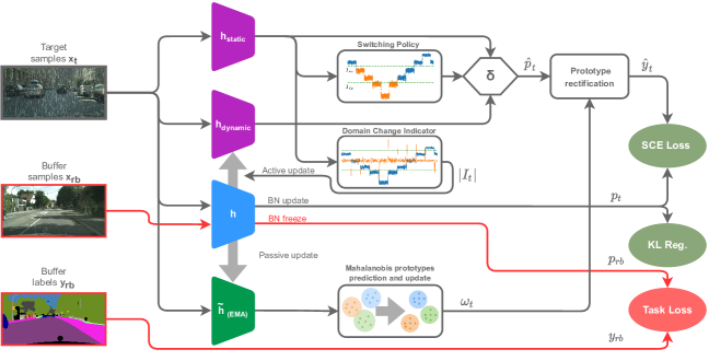
Figure 2: Overview of our OnDA framework. It comprises Switching Policy, Domain Change Indicator, Mahalanobis prototypes prediction, and BN freezing.

We now introduce the design of a prototypical framework for the online setting.

Replay Buffer. First of all, in order to simulate a realistic deployment, where storing the full source dataset $D_{S}$ might be infeasible, we sample a subset $D_{RB}\subseteq D_{S}$ as a Replay Buffer. The buffer is used for training with segmentation loss during adaptation and prevents the network from forgetting the original domain. As we will show in Section 4.3, even a small buffer is very helpful in the mitigation of catastrophic forgetting.

Problem formulation. We define our network as $h=g\circ f$, where $f$ is the feature encoder mapping images into a space of dimension $K$ and $g$ maps features into class labels. We denote sample-label pair from the source and Replay Buffer as ($x_{s},y_{s}$) and ($x_{rb},y_{rb}$) respectively. We model the target domain $D_{T}$ as a sequence of $\Theta$ sub-domains, such that $D_{T}=(D_{T_{1}},D_{T_{2}},...,D_{T_{\Theta}})$.

Prototypes initialization. In online scenarios target samples appear sequentially ($x_{t}^{(1)},x_{t}^{(2)},...,x_{t}^{(N)}$) and it is unknown from which $D_{T_{\theta}}$ they have been sampled. Therefore, target samples can not be used to initialize the class prototypes before the adaptation process takes place. To address this limitation, we initialize the prototypes using the source dataset and update them on the fly using target samples. Letting $h_{\text{static}}=g_{\text{static}}\circ f_{\text{static}}$ be the network fully trained on $D_{S}$ before adaptation, the prototype initialization $\eta^{c}\in\mathbb{R}^{K}$ for each class $c$ is given by:

$$\eta^{c}=\frac{1}{\left|\Lambda_{\mathbf{S}}^{c}\right|}\sum_{i=1}^{N_{S}}\sum_{j}^{H\times W}\left(y_{s}^{(i)}|_{j}=c\right)\left.f_{\text{static}}\left(x^{(i)}_{s}\right)\right|_{j}$$ (1)

where $N_{S}$, $H$, $W$ are the number of source samples, image height and image width respectively. $\left|\Lambda_{\mathbf{S}}^{c}\right|$ denotes the number of pixels that belong to class $c$ from set S, and $\left|\Lambda_{\mathbf{S}}\right|=\sum_{c}\left|\Lambda^{c}_{\mathbf{S}}\right|$. The variance $\sigma\in\mathbb{R}^{K}$ of each dimension $k$ of the prototype space is then obtained through:

$$\sigma^{2}=\frac{1}{\left|\Lambda_{\mathbf{S}}\right|}\sum_{i=1}^{N_{S}}\sum_{j}^{H\times W}\left.{f_{\text{static}}\left(x^{(i)}_{s}\right)}^{2}\right|_{j}-\left(\frac{1}{\left|\Lambda_{\mathbf{S}}\right|}\sum_{i=1}^{N_{S}}\sum_{j}^{H\times W}\left.f_{\text{static}}\left(x^{(i)}_{s}\right)\right|_{j}\right)^{2}$$ . (2)

Hence, given a target sample $x_{t}$, we obtain the prediction $\omega_{t}^{c}$ as the softmax of the variance-normalized proximity between prototypes $\eta$ and the momentum encoder prediction $\tilde{f}\left(x_{t}\right)$,

$$\omega_{t}^{c}=\frac{\exp\left(-\left\|\left(\tilde{f}\left(x_{t}\right)-\eta^{c}\right)/\sigma\right\|\right)}{\sum_{c^{\prime}}\exp\left(-\left\|\left(\tilde{f}\left(x_{t}\right)-\eta^{c^{\prime}}\right)/\sigma\right\|\right)}$$ (3)

where $\tilde{h}=\tilde{g}\circ\tilde{f}$ is the momentum model of the network $h$. The momentum encoder $\tilde{f}$ is used to produce stable predictions compared to using the main encoder $f$ directly and it is created by exponentially averaging the parameters of $f$ over time. In Eq. 3, we employ a form of Mahalanobis distance, including the variances in each dimension of the feature vector. Compared to the Euclidean distance, this leads to a more accurate measure of the distance and higher overall metrics (+4.5% mIoU in the hardest target domain).

Prototypes update. During the adaptation, the prototypes are updated online through target samples pseudo-labeling. Given a batch of $N$ target samples $B$, the batch prototypes are defined as follows:

$$\hat{\eta}^{c}=\frac{1}{\left|\Lambda_{\mathbf{B}}^{c}\right|}\sum_{i=1}^{N}\sum_{j}^{H\times W}\left(\tilde{h}(x_{t}^{(i)})=c\right)\left.\tilde{f}\left(x^{(i)}_{t}\right)\right|_{j}.$$ (4)

Then for all classes $c$ where $\left|\Lambda_{\mathbf{B}}^{c}\right|>0$ we update the corresponding prototype using $\eta^{c}\longleftarrow\lambda\eta^{c}+(1-\lambda)\hat{\eta}^{c}$. Prototypes are used to lessen the reliance on the source label distribution. Naive pseudo-labeling will produce models that are highly biased towards the most popular and easier classes. In domain adaptation, source and target label distributions do not necessarily align. Feature distance through prototypes, on the other hand, removes class biases and produces unbiased predictions. Finally, the pseudo-label $\hat{y}_{t}$ for a sample $x_{t}$ is computed by rectifying the model prediction using the prototype softmax output $\omega_{t}$ as follows:

$$\hat{y}_{t}=\xi(\hat{p}_{t}\cdot\omega_{t})$$ (5)

where $\xi$ is a function that transforms soft-labels to one-hot encoded hard labels. Moreover, instead of directly using the model prediction $p_{t}=h(x_{t})$, checkpoints of the $h$ model are used. In particular, we define:

$$\hat{p}_{t}=\delta h_{\text{static}}(x_{t})+(1-\delta)h_{\text{dynamic}}(x_{t})$$ (6)

Where $h_{\text{dynamic}}$ is the last adapted model on the previous deployment domain, and $\delta\in[0,1]$ determines the contribution of each model. In Section 3.3 we will describe how to guide the adaptation process by dynamically updating $\delta$.

Overconfidence handling. Self-training is a form of entropy minimization which means that the network will tend to become overconfident. Pseudo-labeling with thresholding strategies alone fail since confidence is no longer a reliable guideline. We utilize loss functions that can withstand overfitting to noisy labels. For this reason, two key techniques are used: confidence regularization and Symmetrical cross-entropy [48]. Given the model prediction $p_{t}=h(x_{t})$ we apply a KL divergence regularizer [62]

$$\mathcal{L}_{\text{reg}}=-\gamma\sum_{k=1}^{K}\frac{1}{K}\log p_{t}.$$ (7)

Moreover, to mitigate the impact of noisy labels we employ Symmetrical Cross-Entropy (SCE). The pseudo-label loss is then described as follows:

$$\mathcal{L}_{\text{pseudo}}=\alpha\ell_{\text{ce}}\left(p_{t},\hat{y}_{t}\right)+\beta\ell_{\text{ce}}\left(\hat{y}_{t},p_{t}\right).$$ (8)

Where $\ell_{\text{ce}}$ is the Cross-Entropy loss, and $\alpha$ and $\beta$ are two weighting hyper-parameters. The complete loss function to perform learning using source and target samples is defined as follows:

$$\mathcal{L}_{\text{total}}=\mathcal{L}_{\text{task}}(x_{rb},y_{rb})+\mathcal{L}_{\text{pseudo}}(x_{t},\hat{y}_{t})+\mathcal{L}_{\text{reg}}(x_{t}).$$ (9)

Batch normalization switching. Batch Normalization (BN) layers [20] are employed to normalize features so as to obtain zero-mean and unit standard deviation distributions by iteratively accumulating statistics after processing any batch. Given features $x_{i}$ for the $i$-th element of the batch, the output $y_{i}$ of any BN layer is computed as $y_{i}=\frac{x_{i}-\mu_{\text{B}}}{\sigma_{\text{B}}}$ with $\mu_{\text{B}},\sigma_{\text{B}}$ being the exponential moving average of the mean and variance of features $x$ respectively. During online adaptation, our network processes data from two different distributions; the samples in the Replay Buffer ($\mathcal{D}_{\text{RB}}$) and those belonging to the target domain distribution ($\mathcal{D}_{T_{\theta}}$). This leads to cumulative statistics not being meaningful as an actual distribution, as already observed in [4, 23]. Hence, we investigate two approaches to batch normalization: i) freezing BN layers when processing samples from $\mathcal{D}_{\text{RB}}$ or ii) swapping BN statistics between $\mathcal{D}_{\text{RB}}$ and $\mathcal{D}_{T_{x}}$. Both turn out to be beneficial in our online settings, thus we selected i) for simplicity. We provide a comparison between the BN approaches in the supplementary material.

3.2 Domain Shift Detection

An essential part of online adaptation is being able to detect the domain shifts and act accordingly. Inspired by the key role of the model confidence as a mean for measuring and minimizing domain shift [45, 43], we use the confidence of $h_{\text{static}}$ to identify domain changes as well as the “direction” of such a change. In online settings, it is indeed crucial to both recognize whether the deployment domain is changing and if the transition is leading towards a more distant domain (forward) or a closer domain (backwards), relatively to the source. Defining $z_{t}$ as the confidence of $h_{\text{static}}$ over the $t$-th batch, expressed as

$$z_{t}=\frac{1}{\left|\Lambda_{\mathbf{B}}\right|}\sum_{i=1}^{N}\sum_{j}^{H\times W}\max_{c}\left.h_{\text{static}}\left(x^{(i)}\right)\right|_{j,c}$$ (10)

we notice clear changes while transitioning between domains (see Figure 2, the Domain Change Indicator, and Sec. 3 of the supplementary material). Therefore, the confidence derivative can be leveraged as an indicator of domain changes and computed using the difference between consecutive values. In order to reduce noise and have a robust representation, a shifting window of length $n$ is used. On each new batch $t$, confidence values ($z_{t}$) are appended to the window, while old ones are removed ($z_{t-n}$). At any given time we compute the weighted average confidence of the window as $\mu_{t}=\frac{1}{n}\sum_{i=0}^{n}w[i]z_{t-i}$, where $w$ is the discrete Hamming window [34] of length $n$. The switching indicator function can then be defined as:

$$I_{t}=\left\{\begin{matrix}[l]\;\;\;1,\;\;\;\;\;\mu_{t}-\mu_{t-1}>T_{\text{cd}}\\ -1,\;\;\;\;\;\mu_{t}-\mu_{t-1}<-T_{\text{cd}}\\ \;\;\;0,\;\;\;\;\;\text{otherwise}\end{matrix}\right.,\;\forall\;t>n+1.$$ (11)

When the window has not been filled yet ($t\leq n+1$), we set $I_{t}=0$. $T_{\text{cd}}$ is a hyperparameter that controls model sensitivity to domain changes. We then detect domain changes by examining the absolute value $|I_{t}|>0$ and their direction studying its sign. In the supplementary material video, we present the behavior of the Domain Change Indicator for much more challenging scenarios, which led us to introduce a simple debouncing window to ensure robust switching.

3.3 Prior model Switching techniques

In this section we will focus on the prior predictions $\hat{p}$ introduced in Eq. 6. In particular, two models are used to acquire the prior: $h_{\text{static}}$ and $h_{\text{dynamic}}$. $h_{\text{static}}$ is the initial model, before any adaptation, while $h_{\text{dynamic}}$ is the model before the adaptation to the current domain takes place. For example, in an adaptation sequence over domains $D_{T_{1}},D_{T_{2}},D_{T_{3}}$, during the first adaptation ($D_{T_{1}}$) the dynamic and static models coincide. As the switching indicator $I_{t}$ perceives that we are moving to the second domain ($D_{T_{2}}$), $h_{\text{dynamic}}$ is updated becoming the model right after the adaptation on $D_{T_{1}}$. Similarly, for the third adaptation (on $D_{T_{3}}$), $h_{\text{dynamic}}$ will become the model after the adaptation on $D_{T_{2}}$ and before $D_{T_{3}}$. The choice of which teacher model is going to be used for the prototypes rectification heavily influence the adaptation capabilities.

In the experimental section, we will show that employing $h_{\text{dynamic}}$ ($\delta=0$) grants extra flexibility, allowing adaptation to harder (i.e. more distant) domains. On one hand, as a drawback, it performs sub-optimally while “adapting back” to previous domains and even $D_{S}$. On the other hand, $h_{\text{static}}$ ($\delta=1$) intrinsically limits adaptation due to its predictions guiding the self-training towards the original model. Nonetheless, it allows for better adaptation in domains closer to $D_{S}$, preventing catastrophic forgetting. We thus identify the need for a mechanism that allows for an effective switching between the two prior models, hence making $\delta$ function of $\mu_{t}$, i.e. $\delta_{t}=Switch(\mu_{t},t)$. We introduce the following policies, summarized in Figure 3:

• Confidence Switch (CS): Applies simple thresholding on the static model confidence $z_{t}$.

  $$\delta^{\text{\text{CS}}}_{t}=\left\{\begin{matrix}[l]1,\;\;\;\;\;\;\;\mu_{t}>T_{c}\\ 0,\;\;\;\;\;\;\;\mu_{t}\leq T_{c}\end{matrix}\right.,\;\;\;\;t\geq 0$$ (12)

• Soft-Confidence Switch (SCS): Performs a Confidence Switch with a smooth transition through a weighted average of the models. By moving farther from the source, i.e. lower confidence, $h_{\text{dynamic}}$ is weighted more, while, when coming back to the source, increases $h_{\text{static}}$ contribution. We define two thresholds $T_{\text{s}}$, $T_{\text{d}}$ with $T_{\text{s}}>T_{\text{d}}$ which indicate the $\mu_{t}$ values where $h_{\text{static}}$ and $h_{\text{dynamic}}$ will be solely used respectively, and we linearly interpolate between the two models when $\mu_{t}$ is in-between the two thresholds. That is:

  $$\delta^{\text{SCS}}_{t}=\max\{\min\{\frac{1}{T_{\text{s}}-T_{\text{d}}}\mu_{t}-\frac{T_{\text{d}}}{T_{\text{s}}-T_{\text{d}}},1\},0\}$$ (13)

• Confidence Derivative Switch (CDS): Uses the indicator function previously described in Section 3.2 to understand if the new domain is farther or closer from the source and selects $h_{\text{dynamic}}$ or $h_{\text{static}}$ accordingly.

  $$\delta^{\text{\text{CDS}}}_{t}=\left\{\begin{matrix}[l]1,\;\;\;\;\;\;\;I_{t}>0\\ 0,\;\;\;\;\;\;\;I_{t}<0\\ \delta^{\text{CDS}}_{t-1},\;\;I_{t}=0\end{matrix}\right.,\;\;\;\;t>0,\;\;\delta_{0}^{\text{CDS}}=1$$ (14)

• Hybrid Switch (HS): Sets two thresholds $T_{c_{A}}$, $T_{c_{B}}$ with $T_{c_{A}}>T_{c_{B}}$ and acts based on confidence values $\mu_{t}$

  $$\delta^{\text{HS}}_{t}=\left\{\begin{matrix}[l]1,\;\;\;\;\;\;\;\;\;\;\;\;\;\;\;\;\;\;\mu_{t}>T_{c_{A}}\\ \delta_{t}^{\text{CDS}},\;\;T_{c_{B}}\leq\mu_{t}\leq T_{c_{A}}\\ 0,\;\;\;\;\;\;\;\;\;\;\;\;\;\;\;\;\;\;\mu_{t}<T_{c_{B}}\end{matrix}\right.,\;\;\;\;t\geq 0$$ (15)

  The Hybrid Switch therefore combines Confidence Switch and Confidence Derivative Switch: it follows the former for high/low $\mu_{t}$, the latter otherwise.

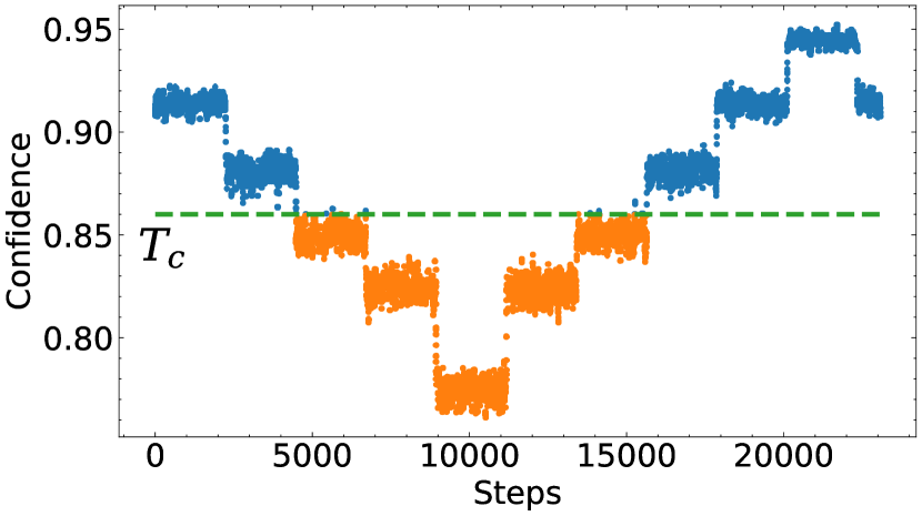
Confidence Switch

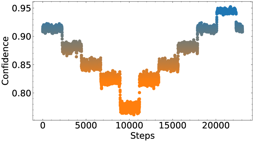
Soft-Confidence Switch

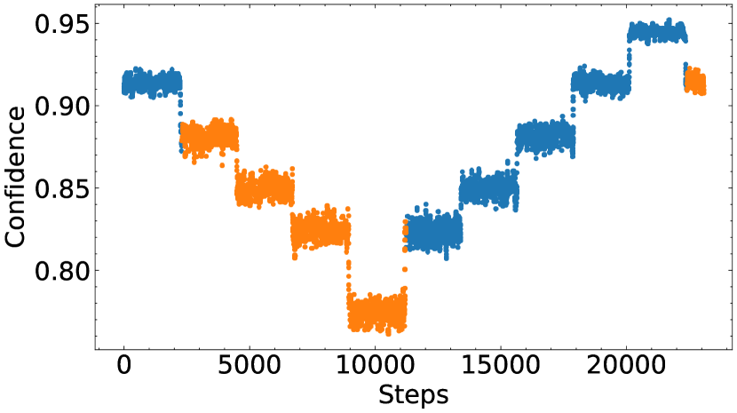
Confidence Derivative Switch

Hybrid Switch

Figure 3: Visualization of the switching policies. The dots show the static models confidence values over time and their color represents $\delta$ values: blue corresponds to $\delta=1$, i.e. $h_{\text{static}}$, while orange $\delta=0$, i.e. $h_{\text{dynamic}}$. The Soft-Confidence Switch performs a linear transition from one prior to the other and it is represented through a color gradient.

4 Experimental Results

The experiments are carried out on the Cityscapes [11] dataset by generating realistic synthetic rain [41]. In particular, we generate a new training set ($2975$ samples) and validation set ($500$ samples) for each rain intensity. Given a pre-trained model on the original dataset, the online adaptation process takes place by training (without labels) on the rain intensities sequentially. After each pass, the model is validated on all rain intensity validation sets. The experiments include severe rain conditions and show how gradual adaptation compares to direct – offline – adaptation.

4.1 Baseline Scenario: Increasing Storm

As baseline scenario, we use rain intensities of $25$, $50$, $75$, $100$ and $200$. Adaptation happens gradually, from low to high intensities, and then backward until clear weather domain, $D_{S}$, is reached again. We will refer to this adaptation sequence, where we move from source to a sequence of targets and eventually return to the source, as an adaptation cycle. Each domain counts about 9K frames – or 5min at 30fps. Harder scenarios will be studied in the remainder.

Experiment Parameters. We use DeepLabv2 [8], which is a common baseline when dealing with domain adaptation on semantic segmentation. The network is although modified to use the ResNet50 [15] feature extractor instead of the DeepLabv2’s default ResNet101 to make training and inference faster. The parameters $\alpha$ and $\beta$ of the SCE are set to $0.1$ and $1$, respectively, while the regularizer parameter $\gamma$ is set to $0.1$. To measure the accuracy of any model, we compute the mIoU metric. Moreover, on the right most column of each table we report the harmonic mean of the overall adaptation process to ease comparison. Our source code is available at https://github.com/theo2021/OnDA.

(a)

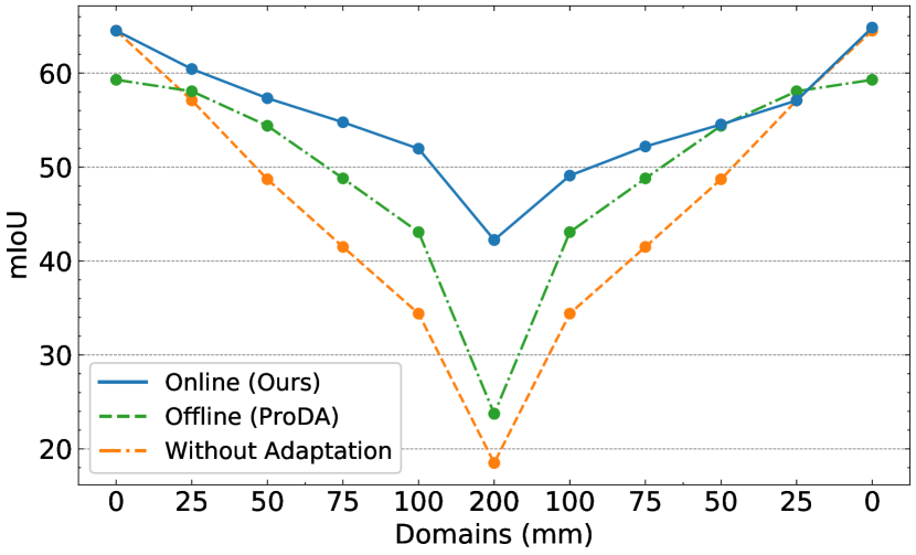
(b)

(c)

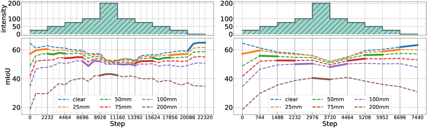
Figure 4: Performance comparison and learning process on Increasing Storm. (a) We plot the mIoU achieved by OnDA using Hybrid Switch (blue), the offline adaptation (green) and the source model (orange), trained on clear weather. The offline model is trained using the source domain, and then adapted to all the rainy domains shown in the $x$ axis at once. In (b), (c) we show for OnDA, at any given time, mIoU of the model in the currently deployed domain with bold segments. The dashed lines show mIoU over past or future domains.

4.2 Results on Increasing Storm

Figure 4, on the left, resumes a direct comparison on the Increasing Storm scenario, between the Source model and those adapted either Offline or Online (with the Hybrid Switch). We can notice a higher mIoU achieved by our framework on any domain. Table 1 showcases more in detail all the major experiments performed, comparing Test-Time/Online Adaptation, Supervised and Offline Adaptation models in the Increasing Storm scenario. In the Offline experiments, we employ a modified version of [56] (Stage 1) which is obtained by adopting the Mahalanobis distance (Eq. 3) and active BN statistics selection 3.1, as these improvements result beneficial also in the traditional offline UDA settings. Training is performed until convergence (10 epochs) with decaying learning rate in a standard setup for both Offline and Supervised models, i.e. they have access – in advance – to the complete data, hence prototypes can be initialized using the target samples. The key comparisons are between adaptations methods, either online or offline and how adaptation compares to the fully supervised, ideal case (oracle). In sum, progressive adaptation sees a significant performance gain compared to directly adapting to a domain offline, as evident by comparing best values (in bold) achieved on each domain. We will now discuss in detail the behavior of the different methods involved in our experiments.

(a) Domain: clear 25mm 50mm 75mm 100mm 200mm h-mean Source Model 64.5 57.1 48.7 41.5 34.4 18.5 37.3 Online (A) BN adaptation 64.5 58.2 51.1 44.8 39.7 27.9 44.3 (B) TENT [46] 64.5 57.1 48.1 41.3 33.6 15.8 35.1 (C) TENT + Replay Buffer 64.5 57.6 50.0 43.8 37.4 20.5 39.7 (D) Online Advent 64.5 58.7 53.5 47.6 43.0 31.1 47.0 (E) OnDA - Static Model 64.5 60.4 57.5 53.5 48.2 37.8 52.0 (F) OnDA - Dynamic Model 64.5 60.4 57.8 54.7 52.7 41.2 54.1 (G) OnDA - Confidence Switch 64.5 60.4 57.5 55.1 51.3 42.1 54.1 (H) OnDA - Confidence Derivative Switch 64.5 60.4 57.1 54.3 52.0 42.4 54.2 (I) OnDA - Soft-Confidence Switch 64.5 60.4 57.4 54.7 52.1 42.3 54.3 (J) OnDA - Hybrid Switch 64.5 60.4 57.3 54.8 52.0 42.2 54.2 (K) OnDA - Hybrid Switch One Pass 64.5 59.5 55.3 52.5 50.3 39.3 52.2		(b) Domain: 100mm 75mm 50mm 25mm clear h-mean Source Model 34.4 41.5 48.7 57.1 64.5 37.3 (A) BN adaptation 39.5 45.1 51.2 58.1 64.4 50.1 (B) TENT [46] 28.5 35.7 43.6 52.7 60.5 41.1 (C) TENT + Replay Buffer 37.3 44.1 50.3 57.7 64.3 48.9 (D) Online Advent 43.3 48.5 54.2 58.9 64.3 52.8 (E) OnDA - Static Model 47.1 50.5 52.3 56.4 64.8 53.6 (F) OnDA - Dynamic Model 49.8 50.1 49.9 50.3 53.3 50.6 (G) OnDA - Confidence Switch 48.3 48.8 52.7 56.0 64.6 53.5 (H) OnDA - Confidence Derivative Switch 50.1 52.5 54.4 56.6 64.7 55.2 (I) OnDA - Soft-Confidence Switch 49.3 49.7 50.1 51.8 64.2 52.5 (J) OnDA - Hybrid Switch 49.1 52.2 54.5 57.1 64.8 55.1 (K) OnDA - Hybrid Switch One Pass 50.2 53.8 56.5 60.1 63.2 56.3
(c) Domain: clear 25mm 50mm 75mm 100mm 200mm h-mean Offline Offline 25mm 62.8 60.2 56.6 51.1 45.7 26.4 46.3 Offline 50mm 60.9 59.0 55.9 51.3 46.4 28.9 47.3 Offline 75mm 58.8 57.2 53.6 48.5 43.8 27.2 45.0 Offline 100mm 55.9 54.6 51.1 46.2 41.8 26.7 43.2 Offline 200mm 49.2 50.7 49.7 47.6 45.0 35.9 45.7 Offline All 59.3 58.1 54.4 48.8 43.1 23.7 43.4 Offline All - Advent 50.8 51.7 49.1 45.9 41.9 30.9 43.6		(d) Domain: clear 25mm 50mm 75mm 100mm 200mm h-mean Supervised Supervised 25mm 63.0 62.4 61.1 58.3 56.7 44.1 56.7 Supervised 50mm 60.4 60.6 60.4 58.2 56.9 47.4 56.9 Supervised 75mm 56.7 58.8 58.6 57.1 56.0 48.4 55.7 Supervised 100mm 56.5 59.0 59.9 58.3 58.0 51.8 57.1 Supervised 200mm 48.9 52.6 54.3 54.5 54.5 51.3 52.6 Supervised All 64.5 64.1 63.7 63.0 62.4 58.2 62.6

Table 1: Domain adaptation main results. Online forward (a), backward (b), Offline (c) and Supervised (d) models are compared. Adaptation happens gradually from low ($25$mm) to high ($200$mm) intensities (a) and backward (b).

Online Adaptation. The simplest way to perform adaptation, is by adjusting the BatchNorm statistics (A) in an online manner. Although simple, it manages to yields significant improvements over the source model. Adaptation using TENT [46] (B) results less effective compared to simply updating BatchNorm statistics, both in forward (a) and backward (b) adaptation. Introducing the Replay Buffer (C) partially improves the results, yet not surpassing (A). Online Advent model (D), which is obtained through the use of the Replay Buffer, increases performance even further, yet resulting less performant than self-training approaches. The Static Model (obtained by fixing $\delta_{t}=1$) (E) is capable of adapting and reverting to the original domain. Nevertheless, we notice that performance in adaptation can be further increased using a dynamic prior ($\delta_{t}=0$) (F) – introduced in Sec. 3.3. Compared to the Static Model (E), the Dynamic Model better adapts to the most challenging domains ($100$ and $200$mm), motivating the need for updating the prior during adaptation. However, the Dynamic Model is more prone to forgetting: Table 1 (b), shows performance while gradually returning to the source domain, i.e. retracing domains in reverse order. The Dynamic Model (F) achieves the worst performance once returned to source domain (clear). This issue is solved by switching between the two priors (G-J). Among the switching policies, the Confidence Derivative (H) and Hybrid (J) perform the best, increasing adaptation performance substantially ($\sim 24\%$mIoU on the hardest domain). Furthermore, all policies managed to regain the initial performance before adaptation – see Table 1 (b). Finally (K) presents the adaptation capabilities of the Hybrid Switch over a 3 times faster Increasing Storm (i.e., happening within fewer frames, as shown in Fig. 4 (c)): while the forward adaptation achieves marginally lower metrics compared to (J), backward adaptation results more effective on average.

Online vs Offline Adaptation. From Table 1 (c), it is evident that Offline methods fall short against Online ones (a), proving that it is harder to adapt to the most challenging domains without intermediate adaptations. We have some evidence of this among the entries in the table. Indeed, the best Offline model results on $75$ and $100$mm domains are achieved by the model adapted on $50$mm, suggesting that, sometimes, adapting to an easier domain can be even preferable compared to direct adaptation to the hardest one. Figure 4 (b, c), outlines the mIoU scores while adapting in an Online manner, on the Increasing Storm setting described so far (b) or by shortening each domain to one third of their length (c). At any time, we also plot the performance for past/future domains (dashed lines). This allows to denote that adapting to close domains (e.g. 50mm) already increases performance to the next to come (75mm, as we can notice from the red dashed line on the left of the bold segment), without yet observing it. Furthermore, the experiment on shorter domains yields similar performance demonstrating, the fast adaptation capabilities of the approach.

Adaptation vs Supervised learning. Although adaptation managed to improve performance, a significant gap between adaptation and supervised learning still exists. Not surprisingly, supervised models perform quite well when fully labelled data is provided, but are always constrained to the source domain, while online adaptation methods can adjust models to new domains on-the-fly.

4.3 Experiments under additional settings

In this section, we extend our evaluation by considering different rainy sequences, by studying the impact of the Replay Buffer and by generalizing our framework to different domain changes, such as increasing fog.

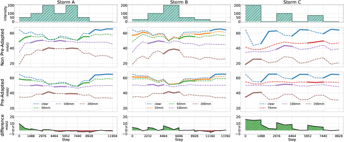
Figure 5: Model performance during adaptation. Experiments on storms A, B & C. Comparison between starting adaptation from source (Non Pre-Adapted) and after a full adaptation cycle on the Increasing Storm (Pre-Adapted).

Evaluation on different Storms. We now run experiments on different rainy scenarios to confirm our previous findings. In particular, we evaluate over three adaptation sequences. In all of them, we use the Hybrid Switch, and we compare two models. The first model is pre-trained on source (clean images), while the second model has already experienced a full adaptation cycle over the Increasing Storm (Section 4.1). Results are collected in Figure 5. On top, we plot histograms describing the three storm intensities, labeled A, B and C and being respectively an oscillatory storm (to evaluate OnDA capability of going back and forth in harder domains), a sudden storm (with a more aggressive intensity growth) and a instantaneous storm (starting with the hardest domain and oscillating significantly). The plots below show the performance of the two models exposed to the same storm. The last row instead shows the mIoU difference between the two. Starting from storm A, we can notice how both models perform similarly and quickly adapt to each domain change. At bootstrap, the pre-adapted model results better, anyway, the non pre-adapted one quickly catches up, eventually closing the gap between the two. The same trend occurs on storm B, although the pre-adapted model results more effective during the whole “forward” pass. By looking at storm C, instead, we witness an interesting behavior. Storm C is by far the most challenging in our benchmark due to its abrupt first intensity. The non pre-adapted model fails to adapt to the $200$mm domain encountered at the very beginning, hinting once again that gradual adaptation is preferable. Indeed, the pre-adapted model can instead easily reach the same performance achieved during the Increasing Storm on just a single pass. This result proves that after an adaptation cycle, the model is not only able to reach again the source domain with no catastrophic forgetting, but, crucially, it also maintains a memory of the previously experienced domains. Hence, it acquires the ability to cope with more challenging and sudden domain shifts. Finally, our supplementary material contains qualitative results and refers to a video, showing OnDA in action on the Increasing Storm scenario.

(a)
		clear		25mm		50mm		75mm		100mm		200mm
Buffer		F	B	F	B	F	B	F	B	F	B	F	B
(A)	0	64.5	57.5	60.5	55.0	57.6	53.5	54.0	50.9	50.1	49.1	41.0	-
(B)	100	64.5	63.0	60.3	56.9	56.2	54.1	54.2	51.6	51.5	49.3	42.9	-
(C)	1000	64.5	64.8	60.4	57.1	57.3	54.5	54.8	52.2	52.0	49.1	42.2	-
(D)	All	64.5	65.4	61.0	55.9	58.1	54.4	53.5	51.1	51.8	49.2	41.4	-

(b)
	Domain (visibility):	clear		750m		375m		150m		75m		h-mean
		F	B	F	B	F	B	F	B	F	B	F	B
	Source	64.9	-	60.9	-	54.7	-	39.8	-	25.2	-	43.5	-
	Offline All	62.4	-	62.3	-	59.6	-	46.8	-	31.9	-	49.2	-
	OnDA - Hybrid Switch	64.9	65.8	63.3	62.3	60.7	58.8	51.6	49.1	42.1	42.1	55.1	54.1

Table 2: Additional experiments. (a): impact of the Replay Buffer on the Increasing Storm cycle using the Hybrid Switch. (b): comparison between Offline and Online adaptation on foggy domains. F: adaptation from clear to the hardest domain, B: backward adaptation (from the hardest domain back to clear).

Ablation Study - Replay Buffer size. We now study the impact of the Replay Buffer size, so far set to $1000$ source samples. Table 2 (a) shows a comparison between different Replay Buffer sizes. The model manages to adapt to hard domains even in the absence of a Replay Buffer (A), this although results to a considerable drop in accuracy in the backward phase (about 10%). With a buffer of $100$ (B) or $1000$ images (C) catastrophic forgetting is solved, while (C) allows for going back to the source with even increased performance. Keeping the whole dataset in the buffer (D) further increases accuracy once back to source, yet not improving adaptation.

Additional Case Study - Fog. Finally, we test the proposed framework on artificially generated fog [41] on the Cityscapes training set. The dataset is randomly split into 2475 training and 500 validation samples and we adopted the same experimental set-up presented in the rain scenario. Table 2 (b) shows a comparison between Source, Offline All and OnDA. Again, our model achieves +10% mIoU on the hardest domain compared to the one adapted offline, confirming that OnDA can be successfully applied to various domain changes.

Limitations. Online training requires significant computational resources, which heavily hinder deployment in real-time applications. We believe that lighter backbones [53], efficient training paradigms [40] or selective adaptation can improve this aspect. From an experimental standpoint, we analyse domain shifts which only affects the input distribution. A larger body of test scenarios, with real data and additional gradual domain shifts would be the ideal stage to assess the performance of OnDA frameworks.

5 Summary & Conclusion

In this paper, we have presented a novel framework for Online Domain Adaptation (OnDA). While state-of-the-art offline adaptation and continuous adaptation methods can successfully tackle limited domain shift, they fall short on cases where there is a significant gap between the source and the deployment domain. In contrast, we have empirically shown that casting adaptation as an online task and gradually adapting to evolving domains are beneficial for reaching high accuracy on distant domains. We exhaustively evaluated our framework on simulated weather conditions with increasing intensity and in four different kinds of storms, highlighting the robustness of our method in comparison to offline techniques. We believe that our framework will pave the way towards tackling UDA in online manner in the real world.

Acknowledgement. The authors thank Hossein Azizpour, Hedvig Kjellström and Raoul de Charette for the helpful discussions and guidance.

Supplementary See pages 1 of onda_supplementary.pdf See pages 2 of onda_supplementary.pdf See pages 3 of onda_supplementary.pdf See pages 4 of onda_supplementary.pdf See pages 5 of onda_supplementary.pdf See pages 6 of onda_supplementary.pdf See pages 7 of onda_supplementary.pdf See pages 8 of onda_supplementary.pdf See pages 9 of onda_supplementary.pdf

References

- [1] Bengio, Y., Louradour, J., Collobert, R., Weston, J.: Curriculum learning. In: Proceedings of the 26th Annual International Conference on Machine Learning. p. 41–48. ICML ’09, Association for Computing Machinery, New York, NY, USA (2009). 10.1145/1553374.1553380, https://doi.org/10.1145/1553374.1553380
- [2] Bobu, A., Hoffman, J., Tzeng, E., Darrell, T.: Adapting to continuously shifting domains. In: ICLR 2018 Workshop Program Chairs (2018), https://openreview.net/forum?id=BJsBjPJvf, 00000
- [3] Cardace, A., Zama Ramirez, P., Salti, S., Di Stefano, L.: Shallow features guide unsupervised domain adaptation for semantic segmentation at class boundaries. In: Proceedings of the IEEE/CVF Winter Conference on Applications of Computer Vision (WACV). pp. 1160–1170 (January 2022)
- [4] Chang, W.G., You, T., Seo, S., Kwak, S., Han, B.: Domain-specific batch normalization for unsupervised domain adaptation. CoRR (2019), http://arxiv.org/abs/1906.03950
- [5] Chen, C., Xie, W., Huang, W., Rong, Y., Ding, X., Huang, Y., Xu, T., Huang, J.: Progressive feature alignment for unsupervised domain adaptation. In: Proceedings of the IEEE/CVF Conference on Computer Vision and Pattern Recognition. pp. 627–636 (2019)
- [6] Chen, L.C., Lopes, R.G., Cheng, B., Collins, M.D., Cubuk, E.D., Zoph, B., Adam, H., Shlens, J.: Naive-student: Leveraging semi-supervised learning in video sequences for urban scene segmentation. In: European Conference on Computer Vision. pp. 695–714. Springer (2020)
- [7] Chen, L.C., Papandreou, G., Kokkinos, I., Murphy, K., Yuille, A.L.: Deeplab: Semantic image segmentation with deep convolutional nets, atrous convolution, and fully connected crfs. IEEE transactions on pattern analysis and machine intelligence 40(4), 834–848 (2017)
- [8] Chen, L.C., Papandreou, G., Kokkinos, I., Murphy, K., Yuille, A.L.: Deeplab: Semantic image segmentation with deep convolutional nets, atrous convolution, and fully connected crfs. IEEE Transactions on Pattern Analysis and Machine Intelligence 40(4), 834–848 (Apr 2018). 10.1109/tpami.2017.2699184, http://dx.doi.org/10.1109/TPAMI.2017.2699184
- [9] Chen, Y.H., Chen, W.Y., Chen, Y.T., Tsai, B.C., Wang, Y.C.F., Sun, M.: No more discrimination: Cross city adaptation of road scene segmenters. In: 2017 IEEE International Conference on Computer Vision (ICCV). pp. 2011–2020. IEEE (2017). 10.1109/ICCV.2017.220, http://ieeexplore.ieee.org/document/8237482/, 00000
- [10] Cicek, S., Soatto, S.: Unsupervised domain adaptation via regularized conditional alignment. CoRR (2019), http://arxiv.org/abs/1905.10885, 00000
- [11] Cordts, M., Omran, M., Ramos, S., Rehfeld, T., Enzweiler, M., Benenson, R., Franke, U., Roth, S., Schiele, B.: The cityscapes dataset for semantic urban scene understanding (2016)
- [12] Dundar, A., Liu, M.Y., Yu, Z., Wang, T.C., Zedlewski, J., Kautz, J.: Domain stylization: A fast covariance matching framework towards domain adaptation. IEEE Transactions on Pattern Analysis and Machine Intelligence pp. 1–1 (2020). 10.1109/TPAMI.2020.2969421
- [13] Furlanello, T., Lipton, Z., Tschannen, M., Itti, L., Anandkumar, A.: Born again neural networks. In: International Conference on Machine Learning. pp. 1607–1616. PMLR (2018)
- [14] Ganin, Y., Ustinova, E., Ajakan, H., Germain, P., Larochelle, H., Laviolette, F., Marchand, M., Lempitsky, V.: Domain-adversarial training of neural networks. The journal of machine learning research 17(1), 2096–2030 (Jan 2016)
- [15] He, K., Zhang, X., Ren, S., Sun, J.: Deep residual learning for image recognition. CoRR abs/1512.03385 (2015), http://arxiv.org/abs/1512.03385
- [16] Hoffman, J., Tzeng, E., Park, T., Zhu, J.Y., Isola, P., Saenko, K., Efros, A., Darrell, T.: CyCADA: Cycle-consistent adversarial domain adaptation. In: Dy, J., Krause, A. (eds.) Proceedings of the 35th International Conference on Machine Learning. Proceedings of Machine Learning Research, vol. 80, pp. 1989–1998. PMLR, Stockholmsmässan, Stockholm Sweden (10–15 Jul 2018)
- [17] Hoffman, J., Wang, D., Yu, F., Darrell, T.: FCNs in the wild: Pixel-level adversarial and constraint-based adaptation. CoRR (2016), http://arxiv.org/abs/1612.02649, 00000
- [18] Hoyer, L., Dai, D., Van Gool, L.: Daformer: Improving network architectures and training strategies for domain-adaptive semantic segmentation. arXiv preprint arXiv:2111.14887 (2021)
- [19] Huang, X., Belongie, S.: Arbitrary style transfer in real-time with adaptive instance normalization. In: Proceedings of the IEEE International Conference on Computer Vision. pp. 1501–1510 (2017)
- [20] Ioffe, S., Szegedy, C.: Batch normalization: Accelerating deep network training by reducing internal covariate shift. In: International conference on machine learning. pp. 448–456. PMLR (2015)
- [21] Iwasawa, Y., Matsuo, Y.: Test-time classifier adjustment module for model-agnostic domain generalization. In: Beygelzimer, A., Dauphin, Y., Liang, P., Vaughan, J.W. (eds.) Advances in Neural Information Processing Systems (2021)
- [22] Kim, M., Byun, H.: Learning texture invariant representation for domain adaptation of semantic segmentation. 2020 IEEE/CVF Conference on Computer Vision and Pattern Recognition (CVPR) (Jun 2020). 10.1109/cvpr42600.2020.01299, http://dx.doi.org/10.1109/cvpr42600.2020.01299
- [23] Klingner, M., Termöhlen, J.A., Ritterbach, J., Fingscheidt, T.: Unsupervised batchnorm adaptation (ubna): A domain adaptation method for semantic segmentation without using source domain representations. In: Proceedings of the IEEE/CVF Winter Conference on Applications of Computer Vision. pp. 210–220 (2022)
- [24] Kuznietsov, Y., Proesmans, M., Van Gool, L.: Towards unsupervised online domain adaptation for semantic segmentation. In: Proceedings of the IEEE/CVF Winter Conference on Applications of Computer Vision. pp. 261–271 (2022)
- [25] Lao, Q., Jiang, X., Havaei, M., Bengio, Y.: Continuous domain adaptation with variational domain-agnostic feature replay. arXiv preprint arXiv:2003.04382 (2020)
- [26] Lee, D.: Pseudo-label : The simple and efficient semi-supervised learning method for deep neural networks. In: Workshop on challenges in representation learning, ICML (2013)
- [27] Li, Y., Yuan, L., Vasconcelos, N.: Bidirectional learning for domain adaptation of semantic segmentation. 2019 IEEE/CVF Conference on Computer Vision and Pattern Recognition (CVPR) (Jun 2019). 10.1109/cvpr.2019.00710, http://dx.doi.org/10.1109/CVPR.2019.00710
- [28] Liang, J., Hu, D., Feng, J.: Do we really need to access the source data? source hypothesis transfer for unsupervised domain adaptation. CoRR (2020), http://arxiv.org/abs/2002.08546
- [29] Liu, Y., Zhang, W., Wang, J.: Source-free domain adaptation for semantic segmentation (2021), http://arxiv.org/abs/2103.16372
- [30] Liu, Y., Kothari, P., van Delft, B.G., Bellot-Gurlet, B., Mordan, T., Alahi, A.: TTT++: When does self-supervised test-time training fail or thrive? In: Beygelzimer, A., Dauphin, Y., Liang, P., Vaughan, J.W. (eds.) Advances in Neural Information Processing Systems (2021)
- [31] Liu, Z., Miao, Z., Pan, X., Zhan, X., Lin, D., Yu, S.X., Gong, B.: Open compound domain adaptation. In: 2020 IEEE/CVF Conference on Computer Vision and Pattern Recognition (CVPR). pp. 12403–12412. IEEE (2020). 10.1109/CVPR42600.2020.01242, https://ieeexplore.ieee.org/document/9157145/
- [32] Mei, K., Zhu, C., Zou, J., Zhang, S.: Instance adaptive self-training for unsupervised domain adaptation. Lecture Notes in Computer Science p. 415–430 (2020)
- [33] Pan, F., Shin, I., Rameau, F., Lee, S., Kweon, I.S.: Unsupervised intra-domain adaptation for semantic segmentation through self-supervision. 2020 IEEE/CVF Conference on Computer Vision and Pattern Recognition (CVPR) (Jun 2020). 10.1109/cvpr42600.2020.00382, http://dx.doi.org/10.1109/cvpr42600.2020.00382
- [34] Poularikas, A.D.: The handbook of formulas and tables for signal processing. The electrical engineering handbook series, CRC Press ; Springer : IEEE Press (1999)
- [35] Sakaridis, C., Dai, D., Hecker, S., Van Gool, L.: Model adaptation with synthetic and real data for semantic dense foggy scene understanding (2018), http://arxiv.org/abs/1808.01265
- [36] Sohn, K., Berthelot, D., Li, C., Zhang, Z., Carlini, N., Cubuk, E.D., Kurakin, A., Zhang, H., Raffel, C.: Fixmatch: Simplifying semi-supervised learning with consistency and confidence. CoRR abs/2001.07685 (2020), https://arxiv.org/abs/2001.07685
- [37] Stan, S., Rostami, M.: Unsupervised model adaptation for continual semantic segmentation. In: AAAI (2021)
- [38] Su, P., Tang, S., Gao, P., Qiu, D., Zhao, N., Wang, X.: Gradient regularized contrastive learning for continual domain adaptation (2020), http://arxiv.org/abs/2007.12942, 00000
- [39] Sun, T., Segu, M., Postels, J., Wang, Y., Van Gool, L., Schiele, B., Tombari, F., Yu, F.: SHIFT: a synthetic driving dataset for continuous multi-task domain adaptation. In: Computer Vision and Pattern Recognition (2022)
- [40] Tonioni, A., Tosi, F., Poggi, M., Mattoccia, S., Stefano, L.D.: Real-time self-adaptive deep stereo. In: Proceedings of the IEEE/CVF Conference on Computer Vision and Pattern Recognition. pp. 195–204 (2019)
- [41] Tremblay, M., Halder, S.S., de Charette, R., Lalonde, J.F.: Rain rendering for evaluating and improving robustness to bad weather. International Journal of Computer Vision (2020)
- [42] Tsai, Y.H., Hung, W.C., Schulter, S., Sohn, K., Yang, M.H., Chandraker, M.: Learning to adapt structured output space for semantic segmentation. 2018 IEEE/CVF Conference on Computer Vision and Pattern Recognition (Jun 2018). 10.1109/cvpr.2018.00780, http://dx.doi.org/10.1109/CVPR.2018.00780
- [43] Vu, T.H., Jain, H., Bucher, M., Cord, M., Pérez, P.: Dada: Depth-aware domain adaptation in semantic segmentation. In: ICCV (2019)
- [44] Vu, T.H., Jain, H., Bucher, M., Cord, M., Perez, P.: Advent: Adversarial entropy minimization for domain adaptation in semantic segmentation. 2019 IEEE/CVF Conference on Computer Vision and Pattern Recognition (CVPR) (Jun 2019). 10.1109/cvpr.2019.00262, http://dx.doi.org/10.1109/CVPR.2019.00262
- [45] Vu, T.H., Jain, H., Bucher, M., Cord, M., Pérez, P.: ADVENT: Adversarial entropy minimization for domain adaptation in semantic segmentation (2019), http://arxiv.org/abs/1811.12833, 00000
- [46] Wang, D., Shelhamer, E., Liu, S., Olshausen, B., Darrell, T.: Tent: Fully test-time adaptation by entropy minimization. In: International Conference on Learning Representations (2021)
- [47] Wang, H., Shen, T., Zhang, W., Duan, L., Mei, T.: Classes matter: A fine-grained adversarial approach to cross-domain semantic segmentation. In: The European Conference on Computer Vision (ECCV) (August 2020)
- [48] Wang, Y., Ma, X., Chen, Z., Luo, Y., Yi, J., Bailey, J.: Symmetric cross entropy for robust learning with noisy labels (2019), http://arxiv.org/abs/1908.06112
- [49] Wu, Z., Han, X., Lin, Y.L., Uzunbas, M.G., Goldstein, T., Lim, S.N., Davis, L.S.: Dcan: Dual channel-wise alignment networks for unsupervised scene adaptation. Lecture Notes in Computer Science p. 535–552 (2018)
- [50] Wu, Z., Wang, X., Gonzalez, J., Goldstein, T., Davis, L.: ACE: Adapting to changing environments for semantic segmentation. In: 2019 IEEE/CVF International Conference on Computer Vision (ICCV). pp. 2121–2130. IEEE (2019). 10.1109/ICCV.2019.00221, https://ieeexplore.ieee.org/document/9009823/
- [51] Wulfmeier, M., Bewley, A., Posner, I.: Incremental adversarial domain adaptation for continually changing environments (2018), http://arxiv.org/abs/1712.07436, 00000
- [52] Yang, Y., Soatto, S.: FDA: Fourier domain adaptation for semantic segmentation. In: 2020 IEEE/CVF Conference on Computer Vision and Pattern Recognition (CVPR). pp. 4084–4094. IEEE (2020). 10.1109/CVPR42600.2020.00414, https://ieeexplore.ieee.org/document/9157228/
- [53] Yu, C., Wang, J., Peng, C., Gao, C., Yu, G., Sang, N.: Bisenet: Bilateral segmentation network for real-time semantic segmentation. In: Proceedings of the European conference on computer vision (ECCV). pp. 325–341 (2018)
- [54] Yuan, Y., Chen, X., Chen, X., Wang, J.: Segmentation transformer: Object-contextual representations for semantic segmentation. In: European Conference on Computer Vision (ECCV). vol. 1 (2021)
- [55] Zhai, X., Oliver, A., Kolesnikov, A., Beyer, L.: S4L: Self-Supervised Semi-Supervised Learning. arXiv e-prints arXiv:1905.03670 (May 2019)
- [56] Zhang, P., Zhang, B., Zhang, T., Chen, D., Wang, Y., Wen, F.: Prototypical pseudo label denoising and target structure learning for domain adaptive semantic segmentation (2021), http://arxiv.org/abs/2101.10979
- [57] Zhang, Q., Zhang, J., Liu, W., Tao, D.: Category anchor-guided unsupervised domain adaptation for semantic segmentation. Advances in Neural Information Processing Systems (2019), http://arxiv.org/abs/1910.13049
- [58] Zheng, Z., Yang, Y.: Unsupervised scene adaptation with memory regularization in vivo. Proceedings of the Twenty-Ninth International Joint Conference on Artificial Intelligence (Jul 2020). 10.24963/ijcai.2020/150, http://dx.doi.org/10.24963/ijcai.2020/150
- [59] Zhu, J.Y., Park, T., Isola, P., Efros, A.A.: Unpaired image-to-image translation using cycle-consistent adversarial networks. 2017 IEEE International Conference on Computer Vision (ICCV) (Oct 2017). 10.1109/iccv.2017.244, http://dx.doi.org/10.1109/ICCV.2017.244
- [60] Zou, Y., Yu, Z., Kumar, B., Wang, J.: Unsupervised domain adaptation for semantic segmentation via class-balanced self-training. In: Proceedings of the European conference on computer vision (ECCV). pp. 289–305 (2018)
- [61] Zou, Y., Yu, Z., Liu, X., Kumar, B.V.K.V., Wang, J.: Confidence regularized self-training. 2019 IEEE/CVF International Conference on Computer Vision (ICCV) (Oct 2019). 10.1109/iccv.2019.00608, http://dx.doi.org/10.1109/ICCV.2019.00608
- [62] Zou, Y., Yu, Z., Liu, X., Kumar, B., Wang, J.: Confidence regularized self-training. In: Proceedings of the IEEE/CVF International Conference on Computer Vision. pp. 5982–5991 (2019)
See pages 1 of onda_supplementary.pdf See pages 2 of onda_supplementary.pdf See pages 3 of onda_supplementary.pdf See pages 4 of onda_supplementary.pdf See pages 5 of onda_supplementary.pdf See pages 6 of onda_supplementary.pdf See pages 7 of onda_supplementary.pdf See pages 8 of onda_supplementary.pdf See pages 9 of onda_supplementary.pdf