Generalizable Patch-Based Neural Rendering
Supplementary Material

A Additional Experiments and Results

A.1 Fine-tuning

While our model is focused at generalizing to unseen scenes, for a thorough comparison against previous methods, we follow the protocol from IBRNet [wang2021ibrnet] and fine-tune our model (for setting 1) on each of the RFF test scenes for 10k iterations. We report the average metrics across all scenes in Table A.1.

Method	PSNR	SSIM	LPIPS
IBRNet [wang2021ibrnet]	26.73	0.851	0.175
GeoNeRF [johari2021geonerf]	26.58	0.856	0.162
Ours	27.66	0.924	0.138

Table A.1: Fine-tuning results on the RFF dataset, setting 1. Our approach not only improves over the baselines on unseen scenes with no re-training as shown in the main paper, but also when allowed to fine-tune for a few iterations on new scenes.

A.2 Number of Reference Views

We train our model with $3,5,7,10$ and $12$ reference images to investigate the effect of number of reference views available to view synthesis. The models are trained on forward-facing scenes from LLFF [mildenhall2019local] and IBRNet [wang2021ibrnet]. We summarize the average performance of each variant on the real-forward-facing dataset in Table A.2. Our model benefits from having access to a large number (up to 10) of reference images.

Number of Reference Views	Real-Forward-Facing
	PSNR	SSIM	LPIPS
3	22.36	0.800	0.286
5	24.33	0.850	0.216
7	25.05	0.860	0.195
10	25.72	0.880	0.175
12	25.69	0.881	0.178

Table A.2: Effect of varying the number of reference view on view-synthesis.

A.3 RGB Prediction

To synthesize a novel view, our model predicts the weights of a linear combination of reference image pixel colors. A common alternative is to combine learned visual features, followed by a learned mapping to color values [suhail21_light_field_neural_render]. To substantiate our argument of better generalization from combining colors instead of features, we train a variant of our model where the output color is predicted from the aggregated features as

$$\mathfrak{c}=\texttt{MLP}\left(\sum\limits_{k=1}^{K}\beta_{k}f_{3}^{k}\right).$$ (1)

We evaluate this approach in setting 1 and show that our model, which combines pixels, is indeed superior. Table A.3 shows the results.

Interpolation Method	Real-Forward-Facing
	PSNR	SSIM	LPIPS
Features	25.08	0.86	0.199
Colors (ours)	25.72	0.88	0.175

Table A.3: Comparison of average performance when using feature versus color interpolation for view-synthesis. Results show that combining the colors of reference views generalizes better than combining visual features.

A.4 DTU to RFF Generalization

We present results on generalization to scenes in the real-forward-facing (RFF) dataset for a model trained only on DTU in Table A.4. While MVSNeRF [Chen_2021_ICCV] has a better PSNR and LPIPS performance our method achieves better SSIM scores on average across all scenes in RFF.

Method	Real-Forward-Facing
	PSNR	SSIM	LPIPS
MVSNeRF	21.93	0.795	0.252
Ours	20.69	0.808	0.281

Table A.4: Generalization results on RFF for a model trained on DTU.

A.5 Timing Statistics

On average, our model trains at around $3.2$ steps per second on $32$ TPUs with a batch size of $4096$. A prior transformer-based neural rendering work, LFNR [suhail21_light_field_neural_render], is slightly faster at $4.2$ steps per second on the same hardware with the same batch size. Rendering one image with our model takes around $15$ seconds whereas LFNR takes around $10$ seconds on the same hardware. While LFNR takes around $16$ hours to train, it can only be trained on single scene. Thus, to render the novel views for the $8$ scenes in the RFF dataset, it would take at least $128$ hours of training plus the inference time. Our model just trains for approximately $24$ hours and can be used for inference directly on all the scenes, albeit with a small drop in rendering quality.

B Quatlitative Results

B.1 DTU Comparison

We compare renderings on the DTU test set against MSVNeRF in Fig. B.1. Compared to MVSNeRF, our model produces renderings with sharper boundaries and textures.

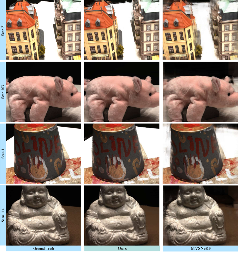
Figure B.1: Qualitative Results on DTU.