MARS : a Method for the Adaptive Removal of Stiffness in PDEs

Abstract

The E(xplicit)I(implicit)N(null) method was developed recently to remove numerical instability from PDEs, adding and subtracting an operator $\mathcal{D}$ of arbitrary structure, treating the operator implicitly in one case, and explicitly in the other. Here we extend this idea by devising an adaptive procedure to find an optimal approximation for $\mathcal{D}$. We propose a measure of the numerical error which detects numerical instabilities across all wavelengths, and adjust each Fourier component of $\mathcal{D}$ to the smallest value such that numerical instability is suppressed. We show that for a number of nonlinear and non-local PDEs, in one and two dimensions, the spectrum of $\mathcal{D}$ adapts automatically and dynamically to the theoretical result for marginal stability. Our method thus has the same stability properties as a fully implicit method, while only requiring the computational cost comparable to an explicit solver. The adaptive implicit part is diagonal in Fourier space, and thus leads to minimal overhead compared to the explicit method.

1 Introduction

Our ability to model many key physical processes is limited by the stability of the numerical schemes we use to simulate the partial differential equations (PDEs) describing them. The reason is that the maximal stable time step of an explicit numerical integration scheme is of the order of the shortest time-scale in the system. In a stable physical system these are typically exponentially damped modes which relax back to equilibrium; the smaller the length scale, the faster the relaxation. This makes it particularly hard to simulate systems at large values of the viscosity or of the surface tension. For instance, surface tension driven flows in the open source fluid dynamics code Gerris [1] (followed by Basilisk :

ttp://basilisk.fr )
require a time step proportional to
$\Delta^{3/2}$\cite{Brackbill1992}, w

ere $\Delta$ is the grid spacing, which this program adapts dynamically in order to ensure a sufficient spatial accuracy [3]. As a result, for small geometries $\Delta$ can be very small, resulting in time steps which are prohibitively small. This constraint is more restrictive than the CFL constraint, related to advection, for which the time step depends on scale like $\Delta$. Another example is the numerical computation of solidification/fusion fronts, which uses a non-linear heat equation [4] : the corresponding time step constraint is $\Delta^{2}$.

If for example relaxation toward equilibrium is controlled by a differential operator of order $m$ ($m=2$ for ordinary diffusion, $m=3$ for the Hele-Shaw flow to be described below), then the required maximum time step $\delta t$ scales as $\delta t=C\delta x^{m}$, where $\delta x$ is the smallest grid spacing or the size of the smallest sub-division. In a well-resolved numerical simulation, this should be considerably smaller than the smallest relevant physical feature. Rapid exponential decay implies that the amplitude of perturbations on the grid scale is very small, and contributes negligible to the numerical solution. Thus one arrives at the paradoxical situation that the stability of the numerical scheme is controlled by a part of the solution which contributes negligibly, and which is actually the most stable from a physical perspective. This property is sometimes referred to as the stiffness of the PDE [5], which becomes worse with increasing spatial order $m$ of the operator.

To deal with this constraint on the time step, which often is so severe that it makes the exploration of important physical parameter regimes impractical, one has to resort to implicit methods. This means that the right hand side of the equation (or at least the stiffest parts of it) has to be evaluated at a future time step, making it necessary to solve an implicit equation at each time step [6, 7]. This makes the numerical code both complicated to write and time-consuming to solve. This is true in particular if the operator is non-local (as is the case for example of integral operators, as they appear in boundary integral type codes [8, 9]). Indeed, in this particular case, when writing an implicit scheme, each element of the discretized solution depends on all the others, requiring a large number of operations to solve the implicit equation.

To address this problem, it has long been realized that not the whole of the right hand side of an equation has to be treated implicitly, as long as the “stiffest” part of the operator is dealt with implicitly. This gives rise to the so-called “implicit-explicit methods” [10, 11], which divide up the problem between explicit and implicit parts, such that hopefully the implicit contribution is sufficiently simple to invert. If this is not clear, as is typically the case for an integral operator, the problem can be solved by judiciously slicing off the stiffest part, which can be local [9]). However, this has to be done on a case-by-case basis, and will not always be possible. Recently, we have presented a much more general method to stabilize stiff equations, which makes use of the arbitrariness in which splitting between explicit and implicit parts can take place [12, 13]. We consider a partial differential equation of the form

$$\frac{\partial u}{\partial t}=f(u,t),$$ (1)

where $u(x,t)$ is a function of space and time or a vector of functions of space and time, and $f(u,t)$ generally is a non-linear operator involving spatial derivatives of $u(x,t)$. In the present article, after explaining the adaptive stabilization procedure in section 2, we shall treat the following three examples :

• A non-linear operator with a fourth-order spatial derivative, related to the thin film flow equation (section 3) :

  $$f(u,t)=-\frac{\partial}{\partial x}\left(u^{3}\frac{\partial^{3}u}{\partial x^{3}}+\frac{1}{u}\frac{\partial u}{\partial x}\right),$$

• A two-dimensional example with a fourth-order derivative (section 4) :

  $$f(u,t)=-\mathcal{N}(u)-\Delta u-\nu\Delta^{2}u,$$

  where $u(x,y,t)$, $\mathcal{N}(u)$ is a non-linear operator, $\Delta$ the Laplacian, and $\nu$ a constant,

• A boundary integral equation (section 5) :

  $$f(u,t)=\int{g(v)K(u,v)}dv,$$

  where $u$ and $v$ are a two-dimensional vectors, $g(v)$ is a function of $v$ involving second-order derivatives in space, $K(u,v)$ is a singular kernel, and the integral is performed along a curve.

As explained in our previous article [13], in order to stabilize the stiff terms in $f(u,t)$, we add two terms on the right-hand-side of the discretized version of equation (1) :

$$\frac{u_{j}^{n+1}-u_{j}^{n}}{\delta t}=f_{j}(u^{n},t^{n})-\mathcal{D}_{j}[u^{n}]+\mathcal{D}_{j}[u^{n+1}],$$ (2)

where $n$ denotes the time variable ($t^{n}=n\delta t$) and $\mathcal{D}$ is an arbitrary operator. The variable $u$ as well as $f$ are defined on a spatial grid $x_{j}=j\delta x$, where $\delta x$ is the grid spacing. Clearly, the added terms are effectively zero apart from the first-order error that comes from the fact that $\mathcal{D}$ is evaluated at different time levels, which motivates the name “Explicit-Implicit-Null” method or “EIN”. If $\mathcal{D}$ is the same as the original operator $f(u,t)$, this is a purely implicit method, if $\mathcal{D}=0$, it is explicit. Similar ideas have been implemented to stabilize the motion of a surface in the diffuse interface and level-set methods [14, 15, 16], and for the solution of PDEs on surfaces [17]. We also show that by a simple step-halving procedure [18], (2) can always be turned into a scheme which is second order accurate in time [13].

When applying (2), we want $\mathcal{D}$ to be a reasonable approximation to the stiff part of $f$. If $\mathcal{D}$ were much larger, it would stabilize the scheme, but would introduce an additional time truncation error. We thus want to choose $\mathcal{D}$ for optimal effectiveness, in the sense that it adds the perfect amount of damping, without adding a supplementary error to the numerical scheme.

This paper presents a numerical scheme to achieve this goal automatically, adjusting $\mathcal{D}$ to the threshold value. Restricting ourselves to periodic boundary conditions, we choose $\mathcal{D}$ to be diagonal in Fourier space, which renders it both simple to handle and sufficiently flexible. Indeed, the implicit step becomes almost trivial to perform:

$$\frac{\hat{u}^{n+1}_{k}-\hat{u}^{n}_{k}}{\delta t}=\hat{f}_{k}(u^{n},t^{n})+\lambda(k)\hat{u}^{n}_{k}-\lambda(k)\hat{u}^{n+1}_{k},$$ (3)

where  $\hat{}$  denotes the Fourier transform and the damping spectrum $\lambda(k)\geq 0$ is an arbitrary function. Adjustment of $\mathcal{D}$ is now down to finding the scalar damping spectrum $\lambda(k)$ for a discrete sequence of $k$’s.

The Fourier transform $\hat{f}_{k}$ can be calculated effectively from the spatial discretization $f_{j}$ using the fast Fourier transform (FFT) [19]. From (3), we find

$$\hat{u}^{n+1}_{k}=\hat{u}^{n}_{k}+\frac{\hat{f}_{k}(u^{n},t^{n})}{\delta t^{-1}+\lambda(k)},$$ (4)

so we obtain the desired solution ${u_{j}}^{n+1}$ at the new time step from the inverse transform. The scheme (4) (as well as any other first order scheme) can be turned into a second order scheme by Richardson extrapolation [18]. Namely, let $u^{1,n+1}$ be the solution for one step $\delta t$, $u^{2,n+1}$ the solution for two half steps $\delta t/2$. Then

$$u^{n+1}=2u^{2,n+1}-u^{1,n+1}+\mathcal{O}(\delta t^{3}),$$ (5)

is second order accurate in time, and

$$E=u^{1,n+1}-u^{2,n+1}$$ (6)

can be used as an error estimator [20].

To analyze (3) further, we adopt a “frozen-coefficient” hypothesis, that the solution is essentially constant over the time scale on which numerical instability is developing. Then assuming small perturbations $\delta\hat{u}_{k}^{n}$, the problem is turned into a linear equation for $\delta\hat{u}_{k}^{n}$, with constant coefficients. At least on a small scale (i.e. in the large $k$ limit), much smaller than any externally imposed scale, $\hat{f}_{k}(u^{n},t^{n})$ is expected to be translationally invariant, making the operator diagonal in Fourier space. Namely, let us assume a more general non-local operator

$$f(x)=\int_{-\infty}^{\infty}D(x,y)u(y)dy.$$

Translational invariance implies that $D(x,y)=D(x-y)$; taking the Fourier transform, we arrive at $\hat{f}(k)=\hat{D}(k)\hat{u}(k)$. This means in the large $k$ limit we expect

$$\hat{f}_{k}(u^{n}+\delta u,t^{n})\sim-e(k)\delta\hat{u}^{n}_{k},$$ (7)

where $\delta u$ is a small perturbation around the solution at $t^{n}$. Here we assume that the eigenvalues $e(k)$ are real, as it is typically the case for physical problems, where the dominant process on a small scale is dissipative.

We have shown in [13] that, as long as $\lambda(k)>e(k)/2$, the system (3) with the approximation (7) is unconditionally stable. This is a generalization of a method first presented, for the case of the diffusion equation in two dimensions, in [21]. If (4) is turned into a second order scheme using (5), this condition is [22] :

$$\lambda(k)>\lambda_{c}(k)=\frac{2}{3}e(k),$$ (8)

with $\lambda_{c}(k)$ the theoretical stability limit. Thus for sufficiently large values of $\lambda(k)$, there is always stability; however, the time truncation error of the second order scheme is $O(\lambda\delta t^{2})$. This is to be compared to the time truncation error $O(e\delta t^{2})$ of the original scheme, and should therefore be kept as small as possible, consistent with the stability constraint. There is a certain similarity here with the preconditioning of matrices, where a matrix is approximated by a simple diagonal matrix [23, 24].

We also showed in [13] that the explicit scheme (i.e. for which $\lambda(k)=0$) is stable as long as :

$$e(k)<\frac{2}{\delta t}.$$ (9)

Equation (9) defines a threshold value of wave numbers $k_{e}$, below which the scheme is stable even without stabilization. As a result, for $k<k_{e}$, $\lambda(k)$ can be chosen to vanish, without affecting stability.

In [13] we have tested the ideas underlying the EIN method, calculating the spectrum $e(k)$ for a variety of operators, including nonlocal operators treated previously in [9]. We approximated $\lambda(k)$ as a power law, derived from the low wavenumber limit of the exact discrete spectrum. As predicted by the above analysis, we find the scheme (3) unconditionally stable, and performing with the same accuracy as that proposed in [9]. Obviously, this still requires one to obtain a good estimate for the spectrum.

In the present paper, we aim to remove this analytical step, and to make the calculation of $\lambda(k)$ self-consistent. The idea is to determine $\lambda(k)$ iteratively, by detecting numerical instability. If, for a given wave number $k$, random perturbations due to numerical instability of the time-stepping grow in time, then the damping is increased, while $\lambda(k)$ can be reduced if the code is stable. In the simplest version of our procedure, we focus on the high wave number limit, where most of the stiffness is coming from, and approximate $\lambda(k)$ by a power law, determined by one or two parameters, depending on whether the exponent is to be prescribed. While we found this approach to work, it introduces arbitrary assumptions into the procedure, and assumes a separation between a high and low wave number regimes. Instead, here we present the results of a scheme which adjusts each Fourier mode individually, based on noise detected in the same Fourier mode. This models the original operator in much greater detail, and leads to a spectrum $\lambda(k)$ which corresponds closely to the theoretical stability limit.

In the next section we develop and describe our procedure for automatic stabilization. The following three sections are each dedicated to a particular example, to illustrate how the method is implemented, and to demonstrate its effectiveness.

2 Adaptive stabilization

Our method is based on the formulation (3), which together with (5) is an unconditionally stable second order scheme, as long as $\lambda(k)$ is sufficiently large. We would like to find an adaptive procedure which refines $\lambda(k)$ at each time step, so as to keep it as small as possible, consistent with stability. To achieve this, we have to address two issues: (i) find a measure $\epsilon(k)$ of the noise, or of numerical instability, for each Fourier mode $k$; (ii) specify the evolution of $\lambda(k)$ for a given noise.

Finding a suitable measure of the error is the crucial question, to be discussed in more detail below. As for (ii), we aim to adjust each Fourier component $\lambda(k)$ individually, although we have also explored representing $\lambda(k)$ by a finite number of parameters. We adopt a simple approach, taking a local relation between $\epsilon(k)$ and $\lambda(k)$, which is shown to be sufficient for the examples to be presented below. For each Fourier mode, if $\epsilon(k)$ is larger than an upper bound $\epsilon_{u}$, the corresponding $\lambda(k)$ is increased by a factor of 1.2. If on the other hand $\epsilon(k)<\epsilon_{u}$, $\lambda(k)$ is decreased slowly by a factor of $1/1.02$ at each time step, in order to avoid a sudden onset of instability. We have used the same rates in all examples, but confirmed that the method is robust against change of parameters.

As to a measure of noise, a first guess might be to take $\epsilon(k)$ as the Fourier transform of the error estimator (6) $\hat{E}_{k}$. We tested this idea using the interface dynamics discussed in more detail in section 5, and illustrated in Fig. 6. Figure 1 shows the evolution of the Fourier transform $\hat{E}_{k}$ of this error estimator, for the first four time steps, without using the EIN method. The time step is chosen to be $\delta t=3.125\times 10^{-5}$, the number of points $N=1024$, and we use a purely explicit scheme (no stabilization), so that the modes with the largest wavenumbers are unstable.

Indeed, as explained in the next sections, there exists a region $k>k_{e}$ in $k$-space which is stable with an explicit scheme (on the left of the vertical dashed line), and an unstable region (on the right), where we would like to detect numerical instability. As a result, the noise level grows very rapidly for the right-hand side of the spectrum, and for the first two time steps there is little power in the $k<k_{e}$ modes. Thus $\hat{E}_{k}$ could be used to detect correctly the numerical instability for large $k$.

However, the left part of the spectrum is soon invaded through non-linear mode-coupling, and there grows a considerable component of the error at small $k$ (corresponding to large scales), which would not be damped away if $\lambda(k)$ was increased. The problem is clear: in the proposed scheme, there is no clean distinction between noise resulting from numerical instability, and the broad spectrum of unstable modes which is part of the physical solution. The crucial problem of defining the numerical noise $\epsilon$ lies in this distinction.

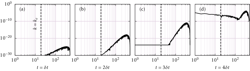
Figure 1: The evolution of the error estimator $\hat{E}_{k}$ (black curve) for the Hele-Shaw flow (27), (28), discussed in more detail in Sect. 5. Initially the error is uniformly small for a flat interface with a white noise. The vertical dashed line is the stability boundary $k=k_{e}$.

A successful procedure came from the idea of spatial smoothing, taking the truncation error as the starting point. To compute $\epsilon$ at the j’th gridpoint, we consider the error estimator $E_{j}$, and compare it to a smoothed version $\bar{E}_{j}$ at the same point. The reasoning is that $\bar{E}_{j}$ contains the full spectrum coming from the deterministic nonlinear dynamics, so $E_{j}-\bar{E}_{j}$ only contains the random noise produced by numerical instability. There are many possible choices for the smoothed-out error. We chose a polynomial approximation over $2n$ gridpoints, but excluding $j$ itself, otherwise $\epsilon$ would be identically zero. In other words,

$$\bar{E}_{j}={\cal P}\left(E_{j-n},\dots,E_{j-1},E_{j+1},\dots,E_{j+n}\right),$$ (10)

where ${\cal P}$ is the $(2n-1)$ degree polynomial, passing through $\left(E_{j-n},\dots,E_{j-1},E_{j+1},\dots,E_{j+n}\right)$. Taking the Fourier transform of the difference between $E_{j}$ and $\bar{E}_{j}$, we define the noise measure $\epsilon(k)$ as

$$\epsilon(k)=\hat{E}_{k}-\hat{\bar{E}}_{k}.$$ (11)

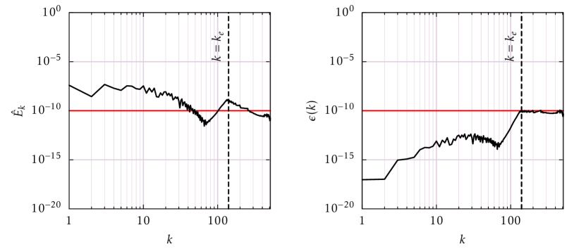
Figure 2: The effect of smoothing on the solution of the Hele-Shaw flow (27),(28) at $t=0.04$, as shown in the third panel of Fig. 6 below. On the left, we show the spectrum of the error estimator $\hat{E}_{k}$, which is broad in the nonlinear regime. On the right, we show the noise measure $\epsilon(k)$ as defined by (11), which is substantial only in a high wave number region where noise is detected. The vertical dashed line is $k=k_{e}$. The horizontal red line is the threshold $\epsilon_{u}$ used to adapt $\lambda(k)$.

The difference between the naive error measure $\hat{E}_{k}$ and $\epsilon(k)$ based on smoothing is illustrated in Fig. 2. We ran the same computation as in figure 1, but using our adaptive procedure. Equation (11) is used as a measure of the noise (with $n=2$) to adapt $\lambda(k)$ at each time step, with the threshold $\epsilon_{u}=10^{-10}$. The left curve shows the Fourier transform $\hat{E}_{k}$ as a function of $k$ : clearly, this error alone is ill-suited to detect instability, since it has significant components for $k<k_{e}$, where the explicit scheme is stable, i.e. where there is no instability even for $\lambda(k)=0$. The right curve shows the noise measure $\epsilon(k)$ given by (11) used to adapt $\lambda(k)$ as a function of $k$ : the instability is correctly detected at large values of $k$ and this error remains low for $k<k_{e}$, i.e. does not require any damping, in the region where an explicit scheme is stable.

3 Example: thin film flow with van der Waals forces

3.1 Equation of motion

As an example of a non-linear equation in one dimension, we first consider a thin liquid film on a horizontal solid substrate. Assuming lubrication theory and taking into account van der Waals forces, which can destabilize the film, the 1D evolution equation for the height of the film $h(x,t)$ reads [25, 26] :

$$\frac{\partial h}{\partial t}=-\frac{\partial}{\partial x}\left(\frac{h^{3}}{3\eta}\frac{\partial}{\partial x}\left[\gamma\frac{\partial^{2}h}{\partial x^{2}}-\frac{A}{6\pi h^{3}}\right]\right),$$ (12)

where $\eta$ is the dynamic viscosity of the fluid, $\gamma$ its surface tension coefficient and $A$ the Hamaker constant. Using $L=\sqrt{A/2\pi\gamma}$ as the lengthscale and $T=3\eta L/\gamma$ as the timescale, the dimensionless equation reads :

$$\frac{\partial h}{\partial t}=-\frac{\partial}{\partial x}\left(h^{3}\frac{\partial^{3}h}{\partial x^{3}}+\frac{1}{h}\frac{\partial h}{\partial x}\right).$$ (13)

Considering the linear stability of (13), we study the growth of a small-amplitude single mode added to an initially flat interface :

$$h(x,t)=h_{0}+\varepsilon e^{ikx+\omega t},$$ (14)

where $x\in[0,1]$. Linearizing equation (13) for $\varepsilon\ll 1$ gives the dispersion relation :

$$\omega=-h_{0}^{3}k^{4}+\frac{k^{2}}{h_{0}}.$$ (15)

As the initial condition, we start from a flat film with a sinusoidal perturbation added to it, corresponding to the most unstable (or Rayleigh) mode. In order to initiate an instability on the scale of the entire computational domain, we fix $k=2\pi$ and set the initial height $h_{0}$ that corresponds to the maximum growth rate :

$$\left.\frac{d\omega}{dk}\right|_{k=2\pi}=0\iff h_{0}=\frac{1}{2^{1/4}(2\pi)^{1/2}}\simeq 0.34$$

Using this initial thickness, we choose as the initial condition :

$$h(x,0)=h_{0}+A\cos(2\pi x),$$ (16)

where $A=0.01$.

In order to compute the right-hand-side $f_{j}(h^{n},t^{n})$ of equation (13), we use second-order centered finite differences on a regular grid $x_{j}=j/N$, where $j\in[0,N]$ and $N=128$ is the number of grid points :

$$f_{j}(h^{n},t^{n})=-h_{j}^{3}\frac{h_{j-2}-4h_{j-1}+6h_{j}-4h_{j+1}+h_{j+2}}{\delta x^{4}}-3h_{j}^{2}\frac{h_{j+1}-h_{j-1}}{2\delta x}\frac{-h_{j-2}+2h_{j-1}-2h_{j+1}+h_{j+2}}{2\delta x^{3}}\\ -\frac{1}{h_{j}}\frac{h_{j+1}-2h_{j}+h_{j-1}}{\delta x^{2}}+\frac{1}{h_{j}^{2}}\left(\frac{h_{j+1}-h_{j-1}}{2\delta x}\right)^{2}.$$ (17)

Using the Fourier transform of (17) in (4), we obtain $\hat{h}^{n+1}_{k}$, from which the new points $h_{j}^{n+1}$ are obtained from the inverse Fourier transform. The Richardson scheme (5), based on each grid point, then leads to a second-order accurate result for $h_{j}^{n+1}$.

3.2 Stabilization

Before proceeding to the automatic stabilization of the numerical scheme, we adopt a von Neumann stability analysis, in order to predict the theoretical value of $\lambda(k)$ for the scheme to be stable. For this purpose, we only need to consider the fourth-order derivative in equation (13), which is the stiff term to be stabilized. Using a “frozen coefficient” hypothesis, we look for perturbations to the mean profile $\overline{h}$ in the form of a single Fourier mode:

$$h_{j}^{n}=\overline{h}(j/N,n\delta t)+\delta\hat{h}_{k}^{n}=\overline{h}(j/N,n\delta t)+\xi^{n}e^{ikj\delta\alpha},$$ (18)

where $\xi(\delta t,k)$ is the amplification factor [27], $\bar{h}$ is assumed constant over the time step, $\delta\alpha=2\pi\delta x=2\pi/N$, and $k\in[0,N-1]$. Inserting this expression into (17), retaining only $-h^{3}h_{xxxx}$ in the original equation, the linearization (7) of the right-hand-side of (13) gives :

$$e(k)=2\frac{\overline{h}^{3}}{\delta x^{4}}\left(\cos(2k\delta\alpha)-4\cos(k\delta\alpha)+3\right).$$ (19)

The modified numerical scheme (4) will be stable as long as $\lambda(k)$ meets the stability criterion (8) with $e(k)$ given by (19). Instead of this $\lambda(k)$, for simplicity we initialize $\lambda(k)$ with an expression of the form $\lambda_{0}k^{4}$, where $\lambda_{0}$ must be chosen as the maximum of $2e(k)/3k^{4}$ over all $k$, in order to satisfy the stability criterion everywhere. It is easily seen that this maximum is attained in the limit $k\rightarrow 0$, from which we obtain

$$\lambda_{0}\geq\frac{32}{3}\pi^{4}\overline{h}^{3}.$$ (20)

Note that (20) depends on the local height $\overline{h}$, which varies slightly for the initial condition; we choose it to correspond to the maximum of the surface elevation, for which the stability requirement is most stringent. In addition, the condition (9) defines a threshold value $k_{e}$, below which the explicit time step is stable’:

$$\frac{2}{\delta t}=e(k)\simeq\overline{h}^{3}(2\pi k_{e})^{4}\Rightarrow k_{e}\simeq\frac{1}{2\pi}\left(\frac{2}{\delta t\;\overline{h}^{3}}\right)^{1/4}\simeq 4.25,$$ (21)

where we have used $\overline{h}=h_{0}=0.34$ and $\delta t=10^{-4}$.

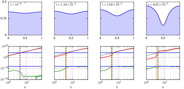
Figure 3: A simulation of the thin film equation with van der Waals forces (13), with the interface shown on the top row. On the lower row, the corresponding spectrum of $\epsilon(k)$ defined by equation (11) (green), as well as $\lambda(k)$ (red). The dotted line is the stability limit $\lambda_{c}(k)=2e(k)/3$, with $e(k)$ given by (19) and $\overline{h}\approx h_{0}$, the top horizontal blue line the explicit stability boundary $2/\delta t$. The vertical dashed line is $k=k_{e}$ given by equation (21), with $\overline{h}=h_{0}$, whereas the vertical orange line is $k=k_{e}$ computed for $\overline{h}=h_{max}$.

Using the procedure described in Sec. 2, for each Fourier mode $\epsilon(k)$ we adjust $\lambda(k)$ depending on whether it is larger or smaller than an upper bound $\epsilon_{u}=10^{-8}$. The value of this bound is subject to some experimentation to make the scheme work, but can be varied by several orders of magnitude without affecting the functioning of the scheme. However, $\epsilon_{u}$ must be chosen in accordance with the typical value of $\epsilon(k)$. Indeed, in the current case, the absolute error (6) is $\mathcal{O}(\delta t^{2})$, and the noise measure (11) introduces a spatial error $\mathcal{O}(\delta x^{2})$, leading to a global absolute error $\mathcal{O}(\delta x^{2}\delta t^{2})\approx 6\times 10^{-13}$, consistent with the green curve in the first panel of figure 3. As a consequence $\epsilon_{u}$ has to be larger than this value for the adaptive procedure to work.

Figure 3 shows our adaptive scheme at work, as the interface (shown on the top row) deforms; the noise measure $\epsilon(k)$ is defined as in (11) (See supplementary movie TF_movie.mpeg). We initialized $\lambda(k)$ to the asymptotic power-law $\lambda_{0}k^{4}$, which is seen as the red line in the lower panel of the first row (which shows the system after the first time step). The true stability boundary, based on the full expression (19), is shown as the dotted line; for small $k$, it is slightly lower than the more stringent power law approximation chosen as the initial condition. The noise measure $\epsilon(k)$ after the first time step is very small as expected.

As seen in the second panel, after some time $\lambda(k)$ has converged onto the theoretical stability limit (8) for small $k$, with $e(k)$ given by (19). Here we have assumed $\overline{h}\approx h_{0}$ for the initial stages of the dynamics, an approximation that will no longer be valid near the end of the computation (fourth row of Figure 3), where $h$ varies considerably in space, and (18) can only be applied locally. However, adjustment of $\lambda(k)$ toward the stability boundary only occurs for $k>k_{e}$, since there is no numerical instability below $k=k_{e}$. As a result, for $k<k_{e}$ the stabilizing spectrum $\lambda(k)$ is reduced at every time step, and in the second panel has already fallen by orders of magnitude below the stability limit of the EIN scheme.

The only source for concern is seen in the 4th panel, when the film thickness has become very non-uniform. In that case there is a region just above $k_{e}$ where $\lambda(k)$ is quite elevated relative to the theoretical limit (but which is based on the assumption of a uniform thickness), as well as noisy. This comes from the fact that the explicit stability boundary $k=k_{e}$ given by (19) moves to the left when values of $h$ in space become significantly higher than $h_{0}$. The vertical orange line in figure 3 corresponds to $k=k_{e}$ computed using the maximum height of the interface $h_{max}$ instead of $h_{0}$. As long as this value does not reach the next smaller integer value of $k$, $\lambda(k)$ is progressively decreased on the left of this boundary. As soon as $k_{e}$ crosses an integer value $k^{\prime}$, exponential growth is observed for $k^{\prime}$ and $\lambda(k^{\prime})$ cannot be adapted quickly enough, resulting in increasing values of $\lambda$ for the adjacent values of $k$. This problem could probably be solved by changing the way $\lambda(k)$ is adapted at each timestep, by testing the stability of each mode and rejecting the timestep in case of instability.

4 Example: 2D Kuramoto–Sivashinsky equation

4.1 Equation of motion

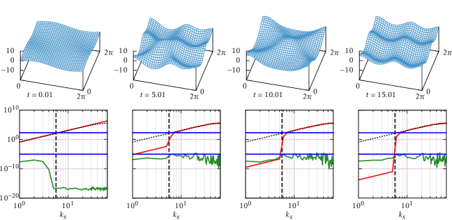
Figure 4: A simulation of the Kuramoto–Sivashinsky equation (22) for $\nu=0.2$, with the interface shown on the top row. $N_{x}=N_{y}=128$ points are used to discretize (22) in both directions, and the time step is $\delta t=0.01$. On the lower row, the corresponding spectrum of $\epsilon(k_{x},0)$ defined by equation (11) (green), as well as $\lambda(k_{x},0)$ (red). The dotted line is the stability limit $\lambda_{c}(k_{x},0)=2e(k_{x},0)/3$ (cf. (24)); the top horizontal blue line the explicit stability boundary $2/\delta t$. The vertical dashed line is $k=k_{e}$ given by $2/\delta t=e_{s}(k_{x},0)$ (cf. (25)); $\lambda(k_{x},k_{y})$ is initialized using $2e_{s}(k_{x},k_{y})/3$. Half of the spectrum in $k_{x}$ is shown, since it is symmetric around $N_{x}/2$ (the other half corresponding to negative wave-numbers $k_{x}\in[-N_{x}/2+1:-1]$).

To demonstrate that our method works in higher dimensions, we consider the example of the 2D Kuramoto–Sivashinsky equation [28], which is known to exhibit spatio-temporal chaos [28, 29] :

$$\frac{\partial u}{\partial t}=-\mathcal{N}(u)-\Delta u-\nu\Delta^{2}u.$$ (22)

The single Laplacian on the right has a minus sign in front of it, leading to instability on the smallest scale; this is stabilized by the last term, which is of forth order, making the problem very stiff. Nonlinearity is introduced through the term

$$\mathcal{N}(u)=\frac{1}{2}\left(|\nabla u|^{2}-\frac{1}{4\pi^{2}}\int_{0}^{2\pi}\int_{0}^{2\pi}|\nabla u|^{2}dxdy\right);$$ (23)

following [29], the spatially constant integral term has been introduced for convenience only, to make sure that $u$ always has zero spatial mean. The variable $u(x,y,t)$ is defined on a two-dimensional square domain, which we can rescale to ensure that $(x,y)\in[0,2\pi]$.

Equation (22) is discretized on a regular grid using centered finite differences in order to find $f_{j_{x},j_{y}}(u^{n},t^{n})$, whose two-dimensional Fourier transform is $\hat{f}_{k_{x},k_{y}}(u^{n},t^{n})$. We can then use the modified time step (4) to find $\hat{u}^{n+1}_{k_{x},k_{y}}$ and thus $u_{j_{x},j_{y}}^{n+1}$. As usual, the scheme is then turned into a second order method using Richardson extrapolation (5). In [29], (22) is treated implicitly using a Fourier pseudospectral method. The purpose of our treatment is to demonstrate the effectiveness of our general scheme, which does not pay attention to the specifics of the operator, in spatial dimensions greater than one.

4.2 Stabilization

In order to study the numerical stability, we only consider the bi-Laplacian, which is the stiffest term to be stabilized. Inserting the single Fourier mode

$$u_{j_{x},j_{y}}^{n}=\xi^{n}e^{i(k_{x}j_{x}\delta x+k_{y}j_{y}\delta y)}$$

into the discretized version of equation (22), and retaining only the bi-Laplacian term, we obtain :

$$e(k_{x},k_{y}) = \nu\left\{\frac{2\cos 2k_{x}\delta x-8\cos k_{x}\delta x+6}{\delta x^{4}}+\frac{2\cos 2k_{y}\delta y-8\cos k_{y}\delta y+6}{\delta y^{4}}\right.$$ (24)

$$+\left.2\frac{2\cos(k_{x}\delta x+k_{y}\delta y)-4\cos k_{y}\delta y+2\cos(k_{x}\delta x-k_{y}\delta y)-4\cos k_{x}\delta x+4}{\delta x^{2}\delta y^{2}}\right\}.$$

The modified numerical scheme (4) will be stable as long as $\lambda(k_{x},k_{y})$ meets the stability criterion (8) : $\lambda(k_{x},k_{y})>2e(k_{x},k_{y})/3$, and the stability of the explicit scheme is given by (9): $e(k_{x},k_{y})<2/\delta t$. For the explicit stability boundary, one can take the small-$k$ limit of (24):

$$e_{s}(k_{x},k_{y})\sim\nu\left(k_{x}^{2}+k_{y}^{2}\right)^{2}.$$ (25)

As in the previous example, this approximation overpredicts the true value of $e(k_{x},k_{y})$ for large wavenumbers. For simplicity, we will use this conservative approximation to set the initial value of $\lambda(k_{x},k_{y})$. The adjustment of $\lambda$ is based on an upper bound $\epsilon_{u}=10^{-5}$ for $\epsilon$. This value is significantly higher than in the previous example, since the typical absolute error in the present case is $\mathcal{O}(\delta x^{2}\delta t^{2})\approx 2\times 10^{-7}$, as seen on the green curve in the first panel of figure 4.

In the definition (6) of $\epsilon(k_{x},k_{y})$, we now have to interpolate the error estimator $E(j_{x},j_{y})$ on a two-dimensional grid; we find $\bar{E}(j_{x},j_{y})$ using a bilinear interpolation of the error estimator :

$$\bar{E}(j_{x},j_{y})=\frac{1}{4}\left[E(j_{x},j_{y}-1)+E(j_{x}+1,j_{y})+E(j_{x},j_{y}+1)+E(j_{x}-1,j_{y})\right]$$ (26)

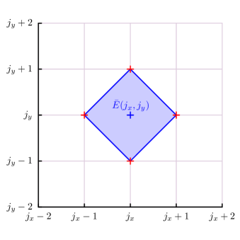
Figure 5: Bilinear interpolation $\bar{E}(j_{x},j_{y})$ using the four neighboring points in red.

Our first attempt was to use $E(j_{x}+1,j_{y}-1)$, $E(j_{x}+1,j_{y}+1)$, $E(j_{x}-1,j_{y}+1)$ and $E(j_{x}-1,j_{y}-1)$ to interpolate $E$ in $(j_{x},j_{y})$, but it turned out that the interpolation values for two adjacent nodes where decoupled, making the process of estimating the error unstable. This issue is addressed by using the four neighbors $E(j_{x},j_{y}-1)$, $E(j_{x}+1,j_{y})$, $E(j_{x},j_{y}+1)$, and $E(j_{x}-1,j_{y})$, as seen in figure 5.

Fig. 4 shows a computation of the Kuramoto–Sivashinsky equation (22), for $\nu=0.2$, in the chaotic regime (See supplementary movie KS_movie.mpeg). Thus the interface $u(x,y)$ deforms in an irregular, unpredictable fashion on many scales. On the lower row we show the corresponding spectrum of $\epsilon(k_{x},0)$ (green), as well as $\lambda(k_{x},0)$ (red). For plotting purpose, we chose to show only a slice of the spectrum ($k_{y}=0$), but the adaption procedure works for the whole 2D spectrum.

We have initialized $\lambda(k_{x},k_{y})$ to $2e_{s}(k_{x},k_{y})/3$ (see (25)). As in the previous example, the initial condition for $\lambda$ (red line) is slightly above the theoretical stability limit (dotted line) for $k$ values corresponding to small scales. This is still true after the first time step, while $\epsilon(k_{x},0)$ is very small as expected. As seen in the second panel, $\lambda(k_{x},0)$ has converged onto the theoretical stability limit $\lambda_{c}(k_{x},0)=2e(k_{x},0)/3$, with $e(k_{x},0)$ given by (24), since the initial condition overpredicts the stability boundary.

However, convergence only occurs for $k>k_{e}$, since below $k=k_{e}$ no numerical instability occurs. As a result, for $k<k_{e}$ the stabilizing spectrum $\lambda(k_{x},0)$ is reduced at every time step, and has already fallen by orders of magnitude below the stability limit of the EIN scheme. Correspondingly, by adjusting $\lambda(k_{x},0)$ the error $\epsilon(k_{x},0)$ is kept close to the threshold $\epsilon_{u}=10^{-5}$ for $k>k_{e}$.

5 Example: Hele–Shaw flow

5.1 Equations of motion

As an example of a non-local, but stiff operator, we consider an interface in a vertical Hele-Shaw cell, separating two viscous fluids with the same dynamic viscosity, with the heavier fluid on top [9]. As heavy fluid falls, small perturbations on the interface grow exponentially: this is known as the Rayleigh-Taylor instability [30]. However, surface tension assures regularity on small scales. For simplicity, we assume the flow to be periodic in the horizontal direction. We briefly recall the dynamics of the interface here; for more details, see [9, 13].

The interface is discretized using marker points labeled with $\alpha$, which represents the motion of a fluid particle. They are advected according to :

$$\frac{\partial{\bf X}(\alpha)}{\partial t}=U{\bf n}+T{\bf s}.$$ (27)

Here ${\bf X}(\alpha)=(x,y)$ is the position vector, ${\bf n}=(-y_{\alpha}/s_{\alpha},x_{\alpha}/s_{\alpha})$ and ${\bf s}=(x_{\alpha}/s_{\alpha},y_{\alpha}/s_{\alpha})$ are the normal and tangential unit vectors, respectively, and $s_{\alpha}=(x_{\alpha}^{2}+y_{\alpha}^{2})^{1/2}$. Hence $U=(u,v)\cdot{\bf n}$ and $T=(u,v)\cdot{\bf s}$ are the normal and tangential velocities, respectively. The tangential velocity does not affect the motion, but is chosen so as to maintain a reasonably uniform distribution of points [9, 13]. If $z(\alpha,t)=x+iy$ is the complex position of the interface, which is assumed periodic with period $1$ ($z(\alpha+2\pi)=z(\alpha)+1$), the complex velocity becomes :

$$u(\alpha)-iv(\alpha)=\frac{1}{2i}PV\int_{0}^{2\pi}{\gamma(\alpha^{\prime},t)\cot\left[\pi(z(\alpha,t)-z(\alpha^{\prime},t))\right]d\alpha^{\prime}},$$ (28)

where $\gamma$ is the vortex sheet strength. For two fluids of equal viscosities [31],

$$\gamma=S\kappa_{\alpha}-Ry_{\alpha},$$ (29)

where $\kappa$ is the mean curvature of the interface :

$$\kappa(\alpha)=\frac{x_{\alpha}y_{\alpha\alpha}-y_{\alpha}x_{\alpha\alpha}}{s_{\alpha}^{3}},\qquad\mathrm{recalling\,\,\,\,that}\qquad s_{\alpha}=(x_{\alpha}^{2}+y_{\alpha}^{2})^{1/2}.$$ (30)

Here $S$ is the non-dimensional surface tension coefficient and $R$ is the non-dimensional gravity force, chosen to be $0.1$ and $50$, respectively, in the following example. To compute the complex Lagrangian velocity of the interface (28), we use the spectrally accurate alternate point discretization [32] :

$$u_{j}-iv_{j}\simeq-\frac{2\pi i}{N}\sum_{{l=0}\atop{j+l\;odd}}^{N-1}{\gamma_{l}\cot\left[\pi(z_{j}-z_{l})\right]}.$$ (31)

Derivatives $\kappa_{\alpha}$ and $y_{\alpha}$ are computed at each time step using second-order centered finite differences, and $\alpha$ is defined by $\alpha(j)=2\pi j/N$, where $j\in[0,N]$ and $N=1024$ is the number of points describing the periodic surface. Note that the numerical effort of evaluating (31) requires $\mathcal{O}(N^{2})$ operations, and thus will be the limiting factor of our algorithm.

5.2 Stabilization

Although the character of the non-local operator in this example is very different from previous equations, our numerical stabilization works in a fashion that is remarkably similar. The modified scheme (4) now becomes

$$\hat{x}^{n+1}_{k}=\hat{x}^{n}_{k}+\frac{\hat{u}_{k}^{n}}{\delta t^{-1}+\lambda(k)},\quad\hat{y}^{n+1}_{k}=\hat{y}^{n}_{k}+\frac{\hat{v}_{k}^{n}}{\delta t^{-1}+\lambda(k)},$$ (32)

where $\hat{u}_{k}^{n}$ and $\hat{v}_{k}^{n}$ are calculated from the Fourier transform of (31). The new grid points $x_{j}^{n+1},y_{j}^{n+1}$ are obtained from the inverse Fourier transform of $\hat{x}^{n+1}_{j},\hat{y}^{n+1}_{j}$, and for each component (32) is turned into a second-order scheme using (5).

In [13], we performed a linear analysis (7) of the discrete modes of (31) about a flat interface. We found that

$$e(k)=\frac{SN^{3}}{L^{3}}\left(1-\cos\frac{2\pi k}{N}\right)\sin\frac{2\pi k}{N}\equiv\tilde{e}(x)=\left(1-\cos x\right)\sin x,\quad x=\frac{2\pi k}{N},$$ (33)

where $L$ is the length of the interface, and $N$ the number of gridpoints. As before, we use the long-wavelength approximation to $e(k)$:

$$e(k)\approx\frac{S}{2L^{3}}(2\pi k)^{3}\equiv e_{s}(x)=\frac{x^{3}}{2},$$ (34)

to find the explicit stability boundary (9) as

$$k_{e}\approx\frac{L}{2\pi}\left(\frac{4}{S\delta t}\right)^{1/3}.$$ (35)

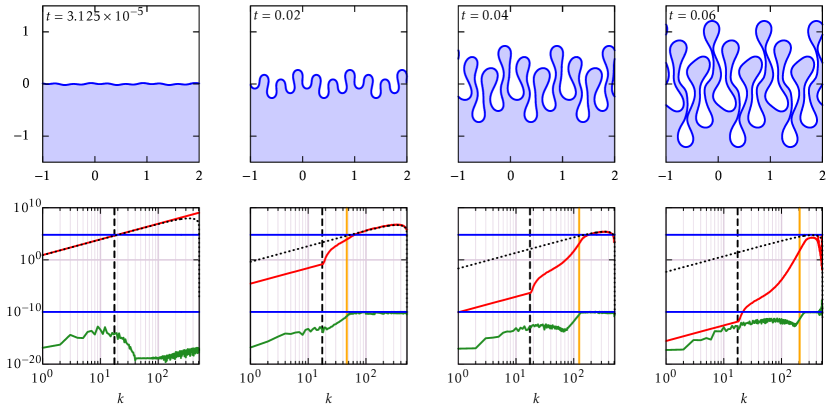
Figure 6: A simulation of the Hele-Shaw problem (27), (28) shown on the top row. On the lower row, the corresponding spectrum of $\epsilon(k)$ defined by equation (37) (green), as well as $\lambda(k)$ (red). The dotted line is the stability limit $\lambda_{c}(k)=2e(k)/3$, with $e(k)$ given by (33), the top horizontal blue line the explicit stability boundary $2/\delta t$. The vertical orange line is $k=k_{e}$ given by equation (35), and the vertical dashed line its initial position.

Using the same approximation (34), which overpredicts the critical value $\lambda(k)$, one finds

$$\lambda_{c}(k)=\frac{S}{3}\left(\frac{2\pi k}{L}\right)^{3}$$ (36)

as a sufficient condition for stability. In [13], we used a fixed spectrum $\lambda(k)$, slightly larger than (36), to stabilize the Hele-Shaw dynamics.

We now use the same procedure as before, with the upper bound $\epsilon_{u}=10^{-10}$ for $\epsilon(k)$. Figure 6 shows our adaptive scheme at work, as the interface (shown on the top row) deforms, and the length $L$ of the interface increases (See supplementary movie HS_movie.mpeg). The error $\epsilon(k)$ is defined as the maximum of (11) over the two components:

$$\epsilon(k)=MAX(\hat{E}^{x}_{k}-\hat{\bar{E}}^{x}_{k},\hat{E}^{y}_{k}-\hat{\bar{E}}^{y}_{k}).$$ (37)

Initializing $\lambda(k)$ to the approximation (36) (red line), we observe the same convergence toward the theoretical stability boundary as before (dotted line). A new feature is that on account of the length $L$ of the boundary increasing in time, the explicit stability boundary $k_{e}$ (vertical dashed and orange lines) increases in time, and the theoretical stability boundary for $\lambda(k)$ (dotted line) comes down. As seen in the second panel of Fig. 6, our adaptive scheme for $k>k_{e}$ has converged toward the theoretical prediction, and then continues to trace it as $L$ increases. The region where no stabilization is required increases as well, and $\lambda(k)$ decreases to very low values on an increasingly large domain. The results described above are not changed significantly as $\epsilon_{u}$ is varied over several orders of magnitude up or down from $10^{-10}$, but of course the value must be significantly over the rounding error, and below the expected truncation error.

In our earlier EIN scheme [13], we used $\lambda(k)$ based on the simplified stability boundary (36) to stabilize the Hele-Shaw interface motion shown in Fig. 6. However, this overpredicts the necessary damping for large $k$. In addition, for $k<k_{e}$, no damping is necessary, and our adaptive scheme reflects that by decreasing $\lambda(k)$ more and more. As a result, the damping in the adaptive scheme is significantly smaller than in our previous EIN scheme. In Fig. 7 we show a comparison of the numerical results to those of the earlier scheme, and find very good agreement. The major advance is of course that $\lambda(k)$ no longer needs to be prescribed, but is found self-consistently as part of the algorithm which ensures stability. Only in the last panel is there a significant discrepancy between the two results. This occurs in places where two sides of the interface have come in close proximity, comparable to the spacing between grid points. But this means our evaluation of the velocity integral is no longer sufficiently accurate to be reliable.

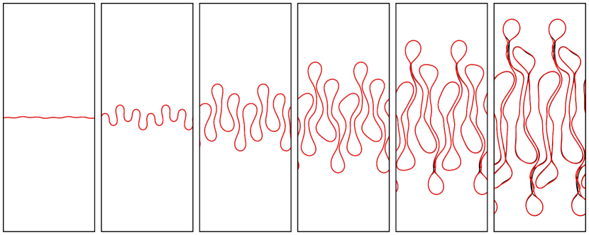
Figure 7: A comparison of the interface as obtained from our current adaptive scheme (red curves) and our earlier EIN scheme (black curves) [13], which used the theoretical stability boundary (36).

6 Outlook and conclusions

We have demonstrated the feasibility of our method using three different model problems, highlighting different aspects of physical problems containing a wide spectrum of time scales, making them stiff. Clearly, there are many ways in which to extend and improve the present approach. Firstly, we estimated the damping spectrum by analyzing the current solution in Fourier space, which is particularly easy for the periodic domain considered by us. However, this may be circumvented by periodically continuing a solution defined over a finite domain only. In addition, one could formulate the entire method in real space, as done in some cases described in [13].

A second, more important issue is our assumption of the spectrum $e(k)$ in (7) being real. This assumption is well founded, since the ultimate physical damping process is dissipative, leading to real eigenvalues. However, as demonstrated by the example of an inertial vortex sheet considered in [9], even problems lacking dissipation can display significant stiffness. This case leads to a system of PDEs, with pairs of complex eigenvalues $e(k)$ on the right-hand-size of (7), corresponding to traveling waves. In that case the damping spectrum $\lambda(k)$ would also have to be complex to ensure stability [13], a case we have not yet considered.

Finally, a problem we still need to address is how to choose an initial condition for the damping spectrum $\lambda(k)$. In the present work we choose a power-law spectrum which can be inferred from a simple analysis of the continuum version of the equations of motion, which then adapts to an optimal spectrum. It would be ideal if no input whatsoever was necessary, choosing for example $\lambda(k)=0$ initially. At present, this is not possible, as the quality of the numerical solution deteriorates before $\lambda(k)$ can adapt. We suspect that in order for such a scheme to be successful, one needs to implement a variable time step, such that initial steps during which $\lambda(k)$ is found are very small.

In conclusion, following our previous study on this subject, we propose a new method to remove the stiffness of PDEs containing non-linear stiff terms, i.e. high spatial derivatives embedded into non-linear terms. This method allows for the self-consistent estimation of a stabilizing term on the right-hand-side of the PDE, that ensures absolute stability for the numerical scheme. Analyzing the spectrum of the solution at each time step, we adapt automatically the stabilizing term such that each unstable Fourier mode is damped optimally. The computational cost of this method is essentially the same as that of the explicit method.

References

- Popinet [2009] S. Popinet, An accurate adaptive solver for surface-tension-driven interfacial flows, J. Comp. Phys. 228 (2009) 5838–5866.
- Brackbill et al. [1992] J. Brackbill, D. B. Kothe, C. Zemach, A continuum method for modeling surface tension, Journal of computational physics 100 (1992) 335–354.
- Popinet [2018] S. Popinet, Numerical models of surface tension, Annual Review of Fluid Mechanics 50 (2018) 49–75.
- Ulvrová et al. [2012] M. Ulvrová, S. Labrosse, N. Coltice, P. Raback, P. Tackley, Numerical modelling of convection interacting with a melting and solidification front: Application to the thermal evolution of the basal magma ocean, Physics of the Earth and Planetary Interiors 206–207 (2012) 51 – 66.
- Kassam and Trefethen [2005] A.-K. Kassam, L. Trefethen, Fourth-order time-stepping for stiff pdes, SIAM J. Sci. Comput. 26 (2005) 1214–1233.
- Iserles [2009] A. Iserles, A first course in the numerical analysis of differential equations, 44, Cambridge university press, 2009.
- Ames [2014] W. F. Ames, Numerical methods for partial differential equations, Academic press, 2014.
- Pozrikidis [1992] C. Pozrikidis, Boundary Integral and singularity methods for linearized flow, Cambridge University Press, Cambridge, 1992.
- Hou et al. [1994] T. Hou, J. Lowengrub, M. Shelley, Removing the stiffness from interfacial flows with surface tension, J. Comp. Physics 114 (1994) 312–338.
- Ascher et al. [1995] U. M. Ascher, S. J. Ruuth, B. T. R. Wetton, Implicit-explicit methods for time-dependent partial differential equations, SIAM J. Numer. Amal. 32 (1995) 797.
- Durran and Blossey [2012] D. R. Durran, P. N. Blossey, Implicit-explicit multistep methods for fast-wave-slow-wave problems, Monthly Weather Rev. 140 (2012) 1307.
- Eggers et al. [1999] J. Eggers, J. R. Lister, H. A. Stone, Coalescence of liquid drops, J. Fluid Mech. 401 (1999) 293–310.
- Duchemin and Eggers [2014] L. Duchemin, J. Eggers, The explicit-implicit-null method: removing the numerical instability of pdes, Journal of Computational Physics 263 (2014) 37–52.
- Smereka [2002] P. Smereka, Semi-implicit level set methods for curvature and surface diffusion motion, J. Sci. Comput. 19 (2002) 439–456.
- Glasner [2003] K. Glasner, A diffuse interface approach to hele-shaw flow, Nonlinearity 16 (2003) 49–66.
- Salac and Lu [2008] D. Salac, W. Lu, A local semi-implicit level-set method for interface motion, J. Sci. Comput. 35 (2008) 330–349.
- Macdonald and Ruuth [2009] C. B. Macdonald, S. J. Ruuth, The implicit closest point method for the numerical solution of partial differential equations on surfaces, SIAM J. Sci. Comput. 31 (2009) 4330–4350.
- Ayati and Dupont [2004] B. P. Ayati, T. F. Dupont, Convergence of a step-doubling galerkin method for parabolic problems, Math. Comput. 74 (2004) 1053–1065.
- Frigo and Johnson [2005] M. Frigo, S. G. Johnson, The design and implementation of FFTW3, Proceedings of the IEEE 93 (2005) 216–231. Special issue on “Program Generation, Optimization, and Platform Adaptation”.
- Hairer et al. [2008] E. Hairer, S. P. Nørsett, G. Wanner, Solving ordinary differential equations I: nonstiff problems, volume 8, Springer Science & Business Media, 2008.
- Douglas Jr. and Dupont [1971] J. Douglas Jr., T. F. Dupont, Alternating-direction Galerkin methods on rectangles, in: B. Hubbard (Ed.), Numerical Solution of Partial Differential Equations II, Academic Press, 1971, pp. 133–214.
- Concus and Golub [1973] P. Concus, G. H. Golub, Use of fast direct methods for the efficient numerical solution of nonseparable elliptic equations, SIAM J. Numer. Anal. 10 (1973) 1103–1120.
- Wathen and Silvester [1993] A. Wathen, D. Silvester, Fast iterative solution of stabilised stokes systems. part i: Using simple diagonal preconditioners, SIAM Journal on Numerical Analysis 30 (1993) 630–649.
- Elman et al. [2014] H. C. Elman, D. J. Silvester, A. J. Wathen, Finite elements and fast iterative solvers: with applications in incompressible fluid dynamics, Numerical Mathematics and Scientific Computation, 2014.
- Williams and Davis [1982] M. B. Williams, S. H. Davis, Nonlinear theory of film rupture, Journal of Colloid and Interface Science 90 (1982) 220–228.
- Zhang and Lister [1999] W. W. Zhang, J. R. Lister, Similarity solutions for van der waals rupture of a thin film on a solid substrate, Physics of Fluids 11 (1999) 2454–2462.
- Press [2007] W. Press, Numerical recipes : the art of scientific computing, Cambridge University Press, Cambridge, UK New York, 2007.
- Cross and Hohenberg [1993] M. C. Cross, P. C. Hohenberg, Pattern formation outside of equilibrium, Rev. Mod. Phys. 65 (1993) 851–1112.
- Kalogirou et al. [2015] A. Kalogirou, E. E. Keaveny, D. T. Papageorgiou, An in-depth numerical study of the two-dimensional kuramoto–sivashinsky equation, Proceedings of the Royal Society A: Mathematical, Physical and Engineering Sciences 471 (2015) 20140932.
- Drazin and Reid [1981] P. G. Drazin, W. H. Reid, Hydrodynamic stability, Cambridge University Press, Cambridge, 1981.
- Majda and Bertozzi [2002] A. J. Majda, A. L. Bertozzi, Vorticity and Incompressible Flow, Cambridge University Press, Cambridge, 2002.
- Shelley [1992] M. Shelley, A study of singularity formation in vortex sheet motion by a spectrally accurate vortex method, J. Fluid Mech. 244 (1992) 493.