Inferring eccentricity evolution from observations of coalescing binary black holes

Abstract

The origin and formation of stellar-mass binary black holes remains an open question that can be addressed by precise measurements of the binary and orbital parameters from their gravitational-wave signal. Such binaries are expected to circularize due to the emission of gravitational waves as they approach merger. However, depending on their formation channel, some binaries could retain a non-negligible eccentricity when entering the frequency band of current gravitational-wave detectors, which will decay as the binary inspirals. In order to meaningfully measure the eccentricity in an observed gravitational-wave signal, two main ingredients are then necessary: an accurate waveform model that describes binaries on eccentric orbits, and an estimator to measure the non-circularity of the orbit as a function of frequency. In this work we first demonstrate the efficacy of the improved TEOBResumS waveform model for eccentric coalescing binaries with aligned spins. We validate the model against mock signals of aligned-spin binary black hole mergers and quantify the impact of eccentricity on the estimation of other intrinsic binary parameters. We then perform a fully Bayesian reanalysis of GW150914 with the eccentric waveform model. We find (i) that the model is reliable for aligned-spin binary black holes and (ii) that GW150914 is consistent with a non-eccentric merger although we cannot rule out small values of initial eccentricity at a reference frequency of $20$ Hz. Secondly, we present a systematic, model-agnostic method to measure the orbital eccentricity and its evolution directly from the gravitational-wave posterior samples. This method mitigates against the contamination of eccentricity measurements through the use of gauge-dependent quantities and has the advantage of allowing for the direct comparison between different analyses, as the definition of eccentricity may differ between models. Our scheme can be applied even in the case of small eccentricities and can be adopted straightforwardly in post-processing to allow for direct comparison between analyses.

I Introduction

Compact binary black holes (BBHs) emit gravitational waves (GWs) during the last stages of their coalescence. During this process the system loses energy and angular momentum, causing the orbit to both shrink and progressively circularize Peters and Mathews (1963). This motivates the analysis of gravitational-wave signals with theoretical templates that are generated by waveform models using the quasi-circular approximation. However, recent studies highlight how accurate measurements of eccentricity can provide vital astrophysical information that could, for example, help discriminate between different binary formation channels Samsing (2018); Rodriguez et al. (2018); Fragione et al. (2019); Samsing et al. (2020); Zevin et al. (2021); Tagawa et al. (2021). Consequently, there has been a growing interest in analyzing the GW events detected by LIGO and Virgo with inspiral-merger-ringdown (IMR) waveform models that include eccentricity  Gayathri et al. (2022); Romero-Shaw et al. (2022); Clarke et al. (2022); Romero-Shaw et al. (2021). For example, the GW transient GW190521 Abbott et al. (2020) has recently been analyzed under the hypothesis that it originated from a hyperbolic capture that resulted in a highly eccentric merger Gamba et al. (2021); other studies claim moderate eccentricity and spin-induced precession as evidence for dynamical formation Romero-Shaw et al. (2020), a possible head-on collision Bustillo et al. (2021) or large eccentricity and strong spin-induced precession Gayathri et al. (2022).

One of the most promising approaches towards modelling the full GW signal emitted by compact binaries on arbitrarily eccentric orbits is the effective-one-body framework (EOB) Buonanno and Damour (1999, 2000); Damour et al. (2000); Damour (2001). Early attempts at incorporating eccentricity within the EOB framework were presented in Hinderer and Babak (2017); Cao and Han (2017); Liu et al. (2019) but have seen numerous improvements over recent years Chiaramello and Nagar (2020); Nagar et al. (2021); Placidi et al. (2021); Albertini et al. (2021); Albanesi et al. (2022a, b); Ramos-Buades et al. (2022); Liu et al. (2021); Yun et al. (2021). In addition to EOB, there have also been numerous developments using alternative approaches towards modelling the complete IMR signal from eccentric binaries, including Numerical Relativity (NR) surrogates Islam et al. (2021); Huerta et al. (2018) and hybrid models that blend post-Newtonian (PN) evolutions with NR simulations Ramos-Buades et al. (2020); Tiwari and Gopakumar (2020); Cho et al. (2021); Chattaraj et al. (2022). A key limitation of these approaches, however, is that they are often constrained by the availability of accurate numerical relativity simulations that span the full parameter space and – in the case of surrogates – by the length of the simulations themselves, which often do not cover the early inspiral of the system. Conversely, models based on analytical PN and scattering calculations Loutrel and Yunes (2017); Loutrel et al. (2019); Moore and Yunes (2019); Boetzel et al. (2019); Klein (2021); Tucker and Will (2021) can deliver representations of signals from long lasting inspirals, but they lack a description of the strong-field merger and are only valid for moderate eccentricities.

We are particularly interested in the TEOBResumS model Nagar et al. (2018, 2020); Riemenschneider et al. (2021) and the extension to eccentricity Chiaramello and Nagar (2020); Nagar et al. (2021); Nagar and Rettegno (2021) that is built on the idea of dressing the circular azimuthal component of radiation reaction with the leading-order (Newtonian) non-circular correction Chiaramello and Nagar (2020). This approach has been subsequently extended to each multipole in the waveform and was further improved by incorporating higher order post-Newtonian information in an appropriately factorized and resummed form Placidi et al. (2021). In particular, Placidi et al. (2021) extended the noncircular waveform up to 2PN using results that partially build on Khalil et al. (2021). Whilst several proposals exist for incorporating radiation reaction, a detailed survey of these schemes was conducted in Albanesi et al. (2022a) concluding that the Newtonian factorization complete with 2PN corrections demonstrated the best agreement with results in the test-mass limit. This paradigm was further extended in Albanesi et al. (2022b).

In this work we focus on TEOBResumS and study the performance of its circular and eccentric versions (TEOBResumS-GIOTTO and TEOBResumS-Dalí, respectively) when applied to GW parameter estimation. We do so with the aim of validating the model and gauging possible biases due to eccentricity (or lack thereof). We dedicate special attention to the study of the quasi circular limit of TEOBResumS-Dalí, and investigate how its structural differences with respect to TEOBResumS-GIOTTO – quantified in terms of unfaithfulness against numerical relativity waveforms – reflect on GW data analysis of synthetic signals and GW150914. We then introduce a method to estimate the eccentricity directly from GW observations and determine its evolution as a function of frequency. This procedure is efficient and suitable to be applied to any eccentric waveform model in post-processing. Furthermore it is advantageous for comparing different eccentric analysis of GW events.

The paper is organized as follows: In Sec. II we summarize the main elements of the EOB waveform model used here. In Sec. III we present a brief review of the elements of Bayesian inference needed for our analysis. Section IV is devoted to the validation of the waveform model via specific injection and recovery analyses. The model is then used to analyze GW150914 data in Sec. V and Sec. VI is dedicated to presenting our method to estimate the eccentricity evolution of a coalescing BBHs system in post-processing. Concluding remarks are reported in Sec. VII. Throughout we use $G=c=1$ unless stated otherwise.

II Quasi-circular and eccentric waveform model: TEOBResumS

All analyses presented in this paper are performed with TEOBResumS, either in its native quasi-circular version, TEOBResumS-GIOTTO Riemenschneider et al. (2021), or in its eccentric version, TEOBResumS-Dalí Nagar et al. (2021). In this section we describe in some detail the features of the two models, highlighting their structural differences and quantifying their (dis-)agreement as measured by the unfaithfulness (or mismatch) defined as:

$$\bar{F}=1-F=1-\underset{t_{0},\phi_{0}}{\rm max}\frac{\langle h_{1}|h_{2}\rangle}{\sqrt{\langle h_{1}|h_{1}\rangle\langle h_{2}|h_{2}\rangle}},$$ (1)

where $(t_{0},\phi_{0})$ are the initial time and phase of coalescence, and $\langle h_{1}|h_{2}\rangle$ is the noise weighted inner product between two waveforms

$$\langle h_{1}|h_{2}\rangle=4\Re\displaystyle\int_{f_{\rm min}}^{f_{\rm max}}\frac{\tilde{h}_{1}(f)\tilde{h}^{*}_{2}(f)}{S_{n}(f)}df,$$ (2)

where $S_{n}(f)$ denotes the power spectral density (PSD) of the detector strain noise and $\tilde{h}_{1}(f)$ and $\tilde{h}_{2}$ are the Fourier transforms of the time domain waveforms $h_{1}$ and $h_{2}$.

II.1 Quasi-circular model: TEOBResumS-GIOTTO

TEOBResumS-GIOTTO is a semi-analytical state-of-the-art EOB model for spinning coalescing compact binaries Damour and Nagar (2014); Nagar et al. (2016, 2018, 2019, 2020); Riemenschneider et al. (2021). The conservative sector of the model includes analytical Post-Newtonian (PN) information, resummed via Padé approximants. Spin-orbit effects are included in the EOB Hamiltonian via two gyro-gravitomagnetic terms Damour and Nagar (2014), while even-in-spin effects are accounted for through the centrifugal radius Damour and Nagar (2014). Numerical Relativity (NR) data is used to inform the model through an effective 5PN orbital parameter, $a_{6}^{c}$, and a next-to-next-to-next-to leading order (NNNLO) spin-orbit parameter, $c_{3}$ Nagar et al. (2018). In the dissipative sector, waveform multipoles up to $\ell=8$ are factorized and resummed according to the prescription of Nagar et al. (2020). Next-to-quasicircular (NQC) corrections ensure a robust transition from plunge to merger, and a phenomenological NR-informed ringdown model completes the model for multipoles up to $\ell\leq 5$. Although we focus here on BBH systems, we note that TEOBResumS-GIOTTO can also generate waveforms for binary neutron star coalescences, see Nagar et al. (2018) and references therein.

Waveforms built from TEOBResumS-GIOTTO employing only the dominant multipole $\ell=|m|=2$ have been tested against the entire catalog of spin-aligned waveforms from the Simulating-eXtreme-Spacetimes (SXS) collaboration SXS , and were shown to be consistently more than $99\%$ faithful to NR Riemenschneider et al. (2021). When higher modes are included in the dissipative sector of the model, the EOB/NR unfaithfulness always lies below the $0.3\%$ threshold when considering waveforms constructed only with the $\ell=|m|=2$ mode, and below $3\%$ for waveforms with modes up to $\ell=4$ if the system has total mass smaller than $120M_{\odot}$ Nagar et al. (2020).

II.2 Eccentric model: TEOBResumS-Dalí

The eccentric generalization of $\tt TEOBResumS$, TEOBResumS-Dalí Chiaramello and Nagar (2020); Nagar et al. (2021), builds on the features of the quasi-circular model detailed above but differs in few key aspects. First, the quasi-circular Newtonian prefactor that enters the factorized waveform multipoles is replaced by a general expression obtained by computing the time-derivatives of the Newtonian mass and current multipoles, as described in Nagar et al. (2021). The same approach is implemented for the azimuthal radiation reaction force. Second, for eccentric binaries, the radial radiation reaction force $\mathcal{F}_{r}$ that contributes to the time evolution of the radial EOB momentum can no longer be neglected Chiaramello and Nagar (2020). Third, the initial conditions must be specified in a different manner with respect to the quasi-circular case: instead of employing the post-adiabatic procedure of Damour et al. (2013), TEOBResumS-Dalí computes adiabatic initial conditions and always starts the evolution of the system at the apastron, see Appendix A for further details. These conservative eccentric initial conditions, however, do not reduce to the quasi-circular initial conditions in the limit of small eccentricity. To partially correct for this issue, the quasi-circular initial conditions are manually imposed for $e_{0}<10^{-3}$. Finally, the values of $a_{6}$ and $c_{3}$ were modified in order to ensure that the model remains faithful to its quasi-circular limit Nagar et al. (2021).

II.2.1 Quasi-circular limit of TEOBResumS-Dalí

All of the modifications above allow TEOBResumS-Dalí to provide waveforms and dynamics that are faithful to mildly eccentric SXS simulations Chiaramello and Nagar (2020); Nagar et al. (2021), scattering angle calculations Nagar et al. (2021) and highly eccentric test-mass waveforms Albanesi et al. (2021). At the same time, however, because of these structural differences, the quasi-circular limit of the eccentric model TEOBResumS-Dalí does not exactly reduce to the TEOBResumS-GIOTTO model. In order to quantify the agreement of TEOBResumS-Dalí with NR simulations and TEOBResumS-GIOTTO, respectively, we calculate the unfaithfulness defined in Eq. (1).

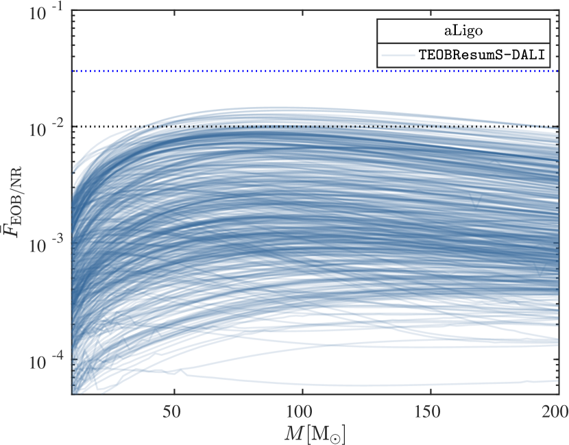
Figure 1: EOB/NR unfaithfulness using TEOBResumS-Dalí with $e_{0}^{\rm inj}=10^{-8}$ over the non-precessing and non-eccentric SXS catalog. See text for more details.

In Fig. 1 we show the unfaithfulness of TEOBResumS-Dalí against almost all. non-eccentric, spin-aligned NR simulations in the SXS catalogue Boyle et al. (2019) using the designed power spectral density (PSD) of Advanced LIGO Buikema et al. (2020). This figure complements, with many more simulations, Fig. 3 of Nagar et al. (2021). Let us remind the reader that the corresponding plot for TEOBResumS-GIOTTO is centered around $10^{-3}$ with $\max(\bar{F}_{\rm EOBNR})\leq 9\times 10^{-3}$ with only a few outliers above $3\times 10^{-3}$ (see Fig. 4 of Riemenschneider et al. (2021)). We thus see here that TEOBResumS-Dalí and TEOBResumS-GIOTTO are two EOB models, similarly informed by NR simulations, that perform differently with respect to quasi-circular NR simulations, though both are clearly below the usual threshold of $3\%$ unfaithfulness. It is therefore interesting to understand how this difference translates in terms of biases on parameters. This will be discussed in Sec. IV.

III Methods

III.1 Bayesian inference

The measurement of the parameters that describe the GW emitting binary is carried out within the framework of Bayesian inference, which relies on Bayes’ theorem Bayes (1764)

$$p(\bm{\theta}|\textbf{d},H)=\frac{p(d|\bm{\theta},H)\,p(\bm{\theta}|H)}{p(\textbf{d}|H)},$$ (3)

where $p(\bm{\theta}|\textbf{d},H)$ is the posterior probability of a set of parameters $\bm{\theta}$ given the data d assuming a specific model $H$, $p(\bm{\theta}|H)$ is the prior, $p(\textbf{d}|\bm{\theta},H)$ is the likelihood and $p(\textbf{d}|H)$ is the evidence or marginalized likelihood. The evidence can be expressed as:

$$Z=p(\textbf{d}|H)=\int\,p(d|\bm{\theta},H)\,p(\bm{\theta}|H)\textbf{d}\bm{\theta},$$ (4)

where the integral extends over the entire parameters space. The evidence assumes the role of an overall normalization constant but plays an important role in Bayesian model selection. Given two competing hypotheses $H_{A}$ and $H_{B}$, the Bayes’ factor is defined as the ratio of evidences

$$\mathcal{B}_{A}^{B}=\frac{p(\textbf{d}|H_{B})}{p(\textbf{d}|H_{A})}\,,$$ (5)

where the hypothesis $H_{B}$ is favoured by the data over $H_{A}$ if $\mathcal{B}_{A}^{B}>1$. The expectation value of a parameter $\theta_{i}\in\bm{\theta}$ can be estimated through the likelihood as

$$E[\theta_{i}]=\int\theta_{i}\,p(\theta_{i}|\textbf{d},H)d\theta_{i},$$ (6)

where $p(\theta_{i}|\textbf{d},H)$ is the marginalized posterior distribution for the parameter $\theta_{i}$.

III.2 Gravitational Wave Parameter Estimation

The GW signal emitted by an eccentric coalescing binary black hole system is fully described by $17$ parameters:

$$\bm{\theta}_{\rm CBC}=\{m_{1},m_{2},\bm{\chi_{1}},\bm{\chi_{2}},D_{L},\iota,\alpha,\delta,\psi,t_{0},\phi_{0},e_{0},f_{0}\},$$ (7)

where $m_{1,2}$ denotes the (detector-frame) masses of the two black holes such that $m_{1}\geq m_{2}$, $\bm{\chi}_{1,2}$ are the dimensionless spin angular momenta vectors with three spatial components, $D_{L}$ is the luminosity distance to the source, $\iota$ is the inclination angle, $\{\alpha,\delta\}$ are the right ascension and declination and define the sky location of the source, $\psi$ is the polarization angle, $\{t_{0},\phi_{0}\}$ are the reference time and phase, and $\{e_{0},f_{0}\}$ are the initial eccentricity magnitude and the average frequency between the apastron and periastron respectively.

In this work we utilize the bajes package for Bayesian inference Breschi et al. (2021) employing the nested sampling Skilling (2006) algorithm dynesty Speagle (2020) in order to extract the posterior probability density functions (PDFs) and to estimate the evidence.

III.2.1 Likelihood

We are interested in the joint likelihood between $N$ detectors in a GW detector network

$$p(\textbf{d}|\bm{\theta},H_{S})=\prod_{i=1}^{N}p(\textbf{d}_{i}|\bm{\theta},H_{S}),$$ (8)

where $H_{S}$ denotes the hypothesis that the data contains a GW signal. Under the assumption of Gaussian, stationary noise that is uncorrelated between each detector, and assuming a time domain signal model $h\equiv h(t,\bm{\theta}_{\rm CBC})$ and data set $d\equiv d(t)$, the likelihood is given by

$$p(\textbf{d}|\bm{\theta}_{\rm CBC},H_{S})\propto e^{-\frac{1}{2}\sum_{i=1}^{N}\langle h-d_{i}|h-d_{i}\rangle},$$ (9)

where $\langle\cdot|\cdot\rangle$ is the noise-weighted inner product as defined in Eq. (2),

$$\langle h-d_{i}|h-d_{i}\rangle=4Re\int_{0}^{\infty}\frac{|\tilde{h}(f)-\tilde{d}_{i}(f)|^{2}}{S_{n}(f)}df,$$ (10)

where $S_{n}(f)$ is the PSD of the detector strain noise, and $\tilde{h}(f)$ and $\tilde{d}$ denote the Fourier transform of $h$ and $d$ respectively.

III.2.2 Priors

For the analyses presented in Sec. IV we adopt priors that broadly follow Abbott et al. (2019); Breschi et al. (2021) and are given as follows:

• The prior distribution for the masses is chosen to be flat in the components masses $\{m_{1},m_{2}\}$ and can be written in terms of the chirp mass $M_{c}=(m_{1}m_{2})^{3/5}/(m_{1}+m_{2})^{1/5}$ and the mass ratio $q={m_{1}}/{m_{2}}\geq 1$ as

  $$p(M_{c},q|H_{S})=\frac{M_{c}}{\Pi_{M_{c}}{\Pi_{q}}}\left(\frac{1+q}{q^{3}}\right)^{2/5},$$ (11)

  where $\Pi_{M_{c}}$ and $\Pi_{q}$ are the prior volumes, as defined in Sec.V B of Breschi et al. (2021) delimited by the prior bounds of $M_{c}$ and $q$.

• To aid the comparison with results from analyses that allow for precessing spins, we assume priors that correspond to the projection of a uniform and isotropic spin distribution along the $\hat{z}$-direction as proposed by Veitch Lange et al. (2018); Breschi et al. (2021):

  $$p(\chi_{i}|H_{S})=\frac{1}{2\chi_{\rm max}}\ln{\Bigg{|}\frac{\chi_{\rm max}}{\chi_{i}}\Bigg{|}},$$ (12)

  where $\chi_{i}$ is the magnitude of each black hole spin and $\chi_{\rm max}$ is the maximum spin magnitude.

• The prior distribution for the luminosity distance $D_{L}$ is specified by a lower and an upper bound and its analytic form is defined by a uniform distribution over the sphere centred around the detectors:

  $$p(D_{L}|H_{S})=\frac{3D_{L}^{2}}{D^{3}_{\rm max}-D^{3}_{\rm min}}$$ (13)

• The prior distributions for $\alpha$ and $\delta$, defining the sky location, are taken to be isotropic over the sky with $\alpha\in[0,2\pi]$, $\delta\in[-\pi/2,+\pi/2]$ and

  $$p(\alpha,\delta|H_{S})=\frac{\cos{\delta}}{4\pi}.$$ (14)

• Analogously, for the inclination we have

  $$p(\iota,H_{S})=\frac{\sin{\iota}}{2},$$ (15)

  where $\iota\in[0,\pi]$.

• For $\{\psi,t_{0},\psi_{0}\}$, the prior distributions are taken to be uniform within the given bounds.

• The prior on $\{e_{0},f_{0}\}$ are taken to be uniform or logarithmic-uniform within the provided bounds that are [0.001, 0.2] and [18, 20.5], respectively.

IV Validation of the waveform model

In this section, we test the consistency of TEOBResumS-Dalí with TEOBResumS-GIOTTO (and vice-versa) by performing Bayesian inference on simulated GW signals (injections). The aim of this analysis is to give a more quantitative meaning to the standard EOB/NR unfaithfulness figures of merit discussed above. To do so, we inject mock signals into a zero noise realization with a signal-to-noise ratio (SNR) of $\sim 42$ in the Advanced LIGO and Advanced Virgo network. We employ the Advanced LIGO and Advanced Virgo design sensitivity PSDs Abbott et al. (2016); Buikema et al. (2020); Acernese et al. (2015). All injections are performed at the same GPS time, $\rm t_{GPS}=1126259462.4$s. We analyze segments of $8$s in duration with a sampling rate of $4096$Hz. We use dynesty to sample the posterior distributions, using the following setting: 3000 live points to initialise the MCMC chains, a maximum of $10^{4}$ MCMC steps, a stopping criterion on the evidence of $\Delta\ln Z=0.1$, and we require five autocorrelation times before accepting a point. For all our analyses, we restrict the waveform model to only the $(2,|2|)$-mode, allowing us to analytically marginalize over the phase.

IV.1 Quasi-circular limit of the eccentric model

As mentioned above, TEOBResumS-Dalí is structurally different to the quasi-circular TEOBResumS-GIOTTO model. Moreover, despite having been informed by the same NR simulations, its unfaithfulness to NR is larger than that of TEOBResumS-GIOTTO. To better understand how this difference in the unfaithfulness translates into parameter biases, we perform an unequal mass injection in the quasi-circular limit, as detailed in Table LABEL:tab:circinj. More precisely, the injected waveform is generated with TEOBResumS-GIOTTO from a fixed initial frequency of 20 Hz, and it is recovered with either the same model (Prior 1) or with TEOBResumS-Dalí assuming a fixed initial eccentricity of $e_{0}=10^{-8}$ at 20 Hz (Prior 2). In Fig. 2 we show the one-dimensional and joint posterior distributions for $M_{c}$, $q$ and the effective spin

$$\chi_{\rm eff}=\frac{m_{1}\chi_{1z}+m_{2}\chi_{2z}}{m_{1}+m_{2}},$$ (16)

where the two spins are taken to be aligned along the $\hat{z}$-direction: $\chi_{1z}=\chi_{1}$ and $\chi_{2z}=\chi_{2}$. The median values of $M_{c}$, $\chi_{\rm eff}$ and $q$ recovered with TEOBResumS-GIOTTO and TEOBResumS-Dalí are shown, with their 90$\%$ credibility interval, respectively in the first and second column of Table 6 in Appendix B. Comparing the results, we notice that the median values of the parameters recovered with TEOBResumS-GIOTTO are in good agreement with the injected ones, while those recovered with the quasi-circular limit of TEOBResumS-Dalí are slightly biased towards higher values. This is not surprising given the different analytical structures (dissipative sectors and NR-informed parameters) of the two models and the fact that TEOBResumS-Dalí is less NR-faithful than TEOBResumS-GIOTTO by, on average, one order of magnitude ($\sim 10^{-2}$ vs. $10^{-3}$) (see Fig. 1 and Fig. 4 of Riemenschneider et al. (2021)). Moreover, when comparing the two models with each other, we also find an average unfaithfulness of $2-3\%$, which increases slightly with the total mass of the binary.

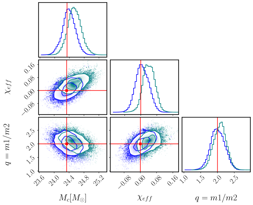
Figure 2: Testing the quasi-circular limit of TEOBResumS-Dalí. We inject a quasi-circular waveform generated with TEOBResumS-GIOTTO and recover it with either TEOBResumS-GIOTTO (blue) or with TEOBResumS-Dalí with fixed initial eccentricity at $e_{0}=10^{-8}$ (teal). The injected values are indicated by the solid lines. We find that the parameters recovered with TEOBResumS-Dalí are slightly biased. See text for discussion.

IV.2 Testing the eccentric model

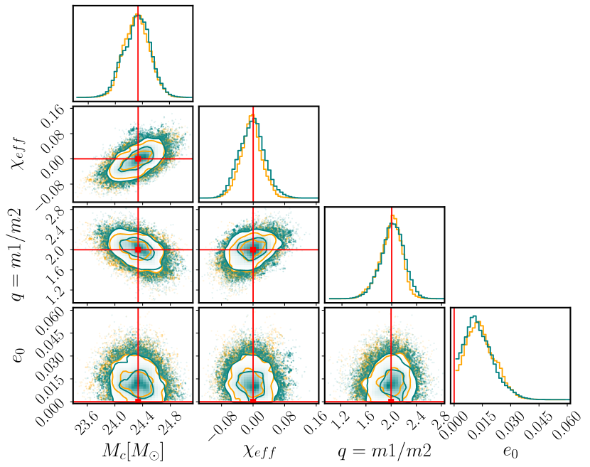
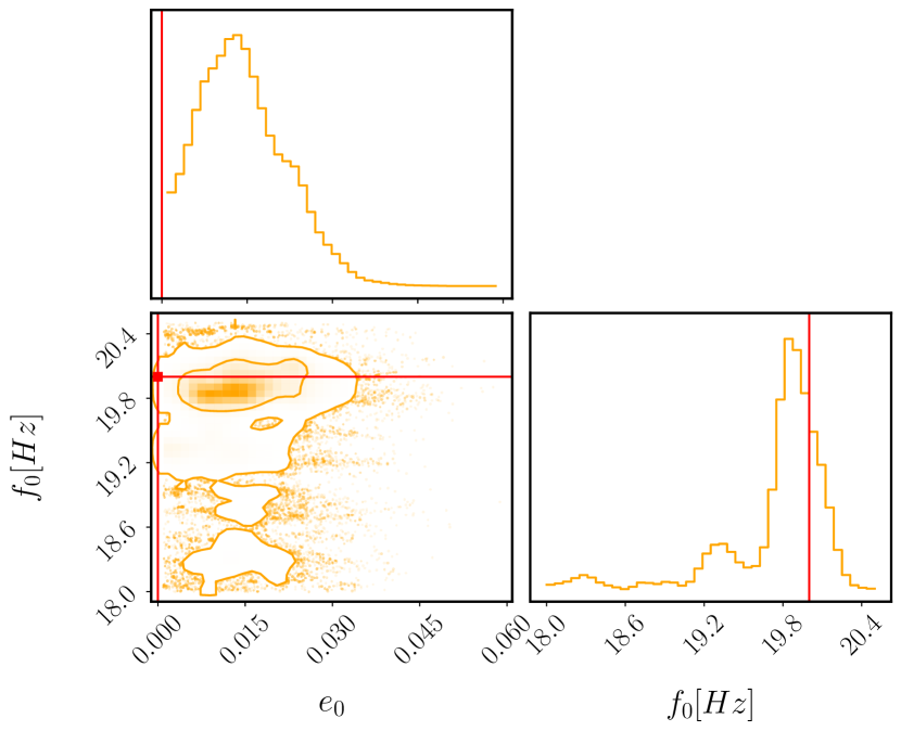
Figure 3: Injection with TEOBResumS-GIOTTO and recovery with TEOBResumS-Dalí. The posterior distributions are obtained by sampling in $(e_{0},f_{0})$ (orange) or by sampling only in $e_{0}$ while keeping $f_{0}$ fixed (teal). The injected values are represented by the solid lines. We do not find appreciable biases in the reconstructed parameters when sampling only in $e_{0}$.

Figure 4: Two-dimensional eccentricity and frequency posterior distributions for the same TEOBResumS-GIOTTO injection and recovery with TEOBResumS-Dalí as in Fig. 4. We do not observe any significant correlation between $e_{0}$ and $f_{0}$.

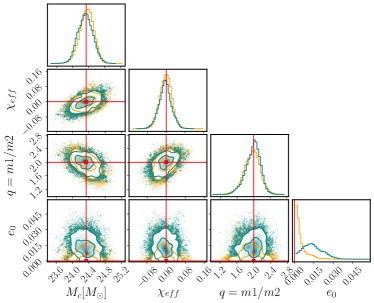
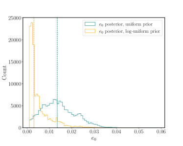
Figure 5: Injection with TEOBResumS-GIOTTO and recovery with TEOBResumS-Dalí. Left: the posterior distribution for the $(M_{c},q,\chi_{\rm eff})$. Right: the posterior distribution for the initial eccentricity using two different choices of priors: uniform (teal) and logarithmic-uniform (orange).

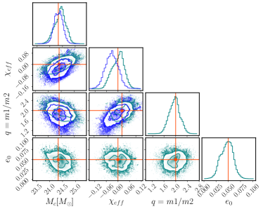
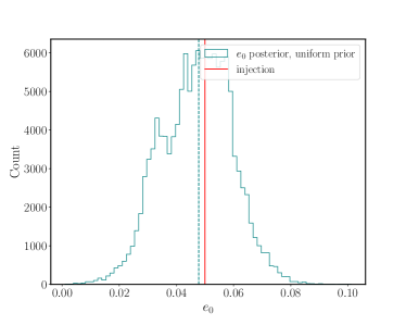
Figure 6: Injection with TEOBResumS-Dalí with fixed EOB eccentricity $e_{0}=0.05$ at $20$ Hz and recovery with TEOBResumS-GIOTTO (blue) or TEOBResumS-Dalí (teal). When the analysis is performed with the latter, all recovered parameters look consistent with the injected ones. Conversely, neglecting eccentricity leads to biases in the mass ratio and effective spin posterior distributions.

In the EOB framework, the dynamics of a system of coalescing binaries is evolved from initial conditions. For the TEOBResumS-Dalí model, this is done by defining an initial eccentricity $e_{0}$ and an initial frequency $f_{0}$ and, through Eq. (19)-(23), determining ($r_{0}$, $p_{\varphi}^{0}$, $p^{0}_{r*}$). The degree to which the initial frequency $f_{0}$ has an impact on Bayesian inference and our ability to constrain this parameter from the observations is poorly understood. In previous similar analyses, comparable quantities, such as the argument of the periapsis or mean anomaly, have typically been ignored. However, recent studies Islam et al. (2021); Romero-Shaw et al. (2022) suggest that the mismatches can degrade as we vary these parameters for a given eccentricity. It is therefore useful to quantify the impact of $f_{0}$ on Bayesian inference. To do so we perform a non-eccentric injection with $e_{0}=0$ and $f_{0}=20$ Hz and recover with TEOBResumS-Dalí either sampling on $e_{0}$ and $f_{0}$ (Prior 1) or only on $e_{0}$ (Prior 2). The details of the injection and the priors are listed in Table LABEL:tab:eccfreq. For the other parameters, the injected values and prior ranges are the same as in Table LABEL:tab:circinj.

Figures 4 and  4 show the one-dimensional and joint posterior distributions obtained with the two different priors. In Fig. 4, we show the posterior distributions for $M_{c}$, $\chi_{\rm eff}$, $q$ and $e_{0}$ obtained using the first prior choice (orange) and the second prior choice (teal). The median values, at $90\%$ credibility, are shown in the third (Prior 1) and fourth (Prior 2) columns of Tab. 6 in App. B. We do not observe any significant differences between the two analyses and we find that the posterior on $f_{0}$ is weakly correlated with $e_{0}$ about its true value as can be seen from Fig. 4. This is in broad agreement with the conclusions of Clarke et al. (2022), who found that the argument of periapsis is only likely to be resolvable for the loudest events. However, as also discussed in Refs. Clarke et al. (2022); Romero-Shaw et al. (2021); O’Shea and Kumar (2021), we could potentially see biases if we fix $f_{0}$ to a frequency that effectively corresponds to the argument of the periapsis being out of phase with the true value. In the $e_{0}\rightarrow 0$ limit, however, one may expect $f_{0}$ to become increasingly degenerate with the coalescence phase.

We note that although the injected value for $e_{0}$ is not contained within the priors, we do not see evidence that this impacts the inferred results. But we find a prior- dependence in the posterior of $e_{0}$ (see Fig. 5 and the discussion below), in addition to the systematic differences between the two models in the circular limit already highlighted in Fig. 2.

We next inject mock signals with two different values of $e_{0}$ and recover them using TEOBResumS-GIOTTO and TEOBResumS-Dalí respectively. The details of the injected values for $e_{0}$ and $f_{0}$ and their priors are described in Table 3. The injected values and priors for the other parameters are the same as before as given in Table LABEL:tab:circinj. Figure 5 shows the one- and two-dimensional posterior distributions for $M_{c}$, $\chi_{\rm eff}$ and $q$ (left) and the one-dimensional posterior distribution for $e_{0}$ (right) for a non-eccentric injection recovered with TEOBResumS-Dalí with two different choices of prior distributions: logarithmic-uniform (teal), uniform (orange). The recovered median values corresponding to the Prior 1 (orange) are shown in the third column while the one corresponding to the Prior 2 (teal) are shown in the fifth column of Tab. 6 in App. B. We observe that for eccentricities comparable to zero, the mass and spin measurements are robust and independent of the choice of eccentricity prior. In the right panel of Fig. 5, we observe that when using a logarithmic-uniform prior for the eccentricity, the recovered median value of the eccentricity is pushed to smaller values as a result of the priors.

In Fig. 6, instead, we show the posterior distributions for an injection with $e_{0}=0.05$ (TEOBResumS-Dalí) and recovered with both the models, TEOBResumS-GIOTTO and TEOBResumS-Dalí. The median values of the parameters recovered with TEOBResumS-GIOTTO (orange) are indicated in the first column of Tab. 7 in App. B, while the ones recovered with TEOBResumS-Dalí (teal) are indicated in the second column of the same Table. In the left figure, we observe a stronger correlation between mass and spin parameters when we recover with TEOBResumS-GIOTTO. Previous studies have pointed out correlations between the chirp mass, the effective inspiral spin and the eccentricity Ramos-Buades et al. (2020); O’Shea and Kumar (2021); Romero-Shaw et al. (2021). As our recovery model neglects eccentricity, biases in the mass and spin parameters are anticipated to compensate for this. Lastly, we draw our attention on the right figure of the bottom panel, where it is shown how excellently the recovery of the eccentricity is accomplished pointing out the robustness and accuracy of the model.

In terms of model selection, we find that for the non-eccentric injection, the recovery with TEOBResumS-GIOTTO is preferred with respect to the one with TEOBResumS-Dalí with an estimated logarithmic Bayes’ factor of $\ln\mathcal{B}_{\rm circ}^{\rm ecc}\sim 9$. Similarly, for the eccentric injection, the eccentric model TEOBResumS-Dalí is preferred with respect to the quasi-circular model TEOBResumS-GIOTTO with an estimated logarithmic Bayes’ factor of $\ln\mathcal{B}_{\rm ecc}^{\rm circ}\sim 5$ in the case of the uniform eccentricity prior, and $\ln\mathcal{B}_{\rm ecc}^{\rm circ}\sim 10$ when using the log-uniform prior. The difference in Bayes’ factor between the two priors can be attributed to the $1/e_{0}$-scaling for the log-uniform prior, which a priori favours smaller values of eccentricity. The investigations presented in this section demonstrate that TEOBResumS-Dalí is a reliable waveform model to analyze spin-aligned, eccentric binaries.

Parameter	Injection 1	Prior 1	Prior 2	Injection 2	Prior 1	Prior 2
$e_{0}$	$0$	$\mathcal{U}(0.001,0.2)$	Log-uniform$(0.001,0.2)$	0.05	$\mathcal{U}(0.001,0.2)$	0 (fixed)
$f_{0}(Hz)$	20	$\mathcal{U}(18,20.5)$	$\mathcal{U}(18,20.5)$	20	$\mathcal{U}(18,20.5)$	20 (fixed)
Model	–	DALI	DALI	DALI	DALI	GIOTTO

Table 3: Second test of TEOBResumS-Dalí with an eccentric recovery. First column: injected values for $e_{0}$ and $f_{0}$ and their prior limits for an injection with $e_{0}=0$ injection recovered with TEOBResumS-Dalí with two different prior choices. Second column: injected values for $e_{0}$ and $f_{0}$ and their prior limits for an injection with $e_{0}=0.05$ recovered with TEOBResumS-Dalí and TEOBResumS-GIOTTO.

V Analysis of GW150914

In this section, we reanalyse GW150914 with the TEOBResumS-Dalí and TEOBResumS-GIOTTO waveform models. The strain data and PSDs are obtained from the GW Open Science Center Trovato (2020). We analyse an $8s$-long data stretch centered around the GPS time of the event $\rm t_{GPS}=1126259462.4\,s$ sampled at a sampling rate of $\rm 4096\,Hz$. For the inference, we use dynesty choosing the same settings discussed in Sec. IV.

V.1 Quasi-circular analysis of GW150914

First, we analyse GW150914 under the assumption of a quasi-circular binary black holes system. To do so, we perform two analyses, either using TEOBResumS-GIOTTO or TEOBResumS-Dalí, fixing initial EOB eccentricity to $e_{0}=10^{-8}$, as described in Table LABEL:tab:circGW150914. In both cases we recover a maximum likelihood SNR of $\sim 26$ corresponding to $\sim 20$ in LIGO-Hanford and $\sim 18$ in LIGO-Livingston. In Fig. 7 we show the marginalized one-dimensional and two-dimensional posterior distributions for $(M_{c},\chi_{\rm eff},q)$ obtained with TEOBResumS-Dalí (teal) and TEOBResumS-GIOTTO (blue). The recovered median values are reported in the second and third column of Table 5. We observe that the values recovered with TEOBResumS-GIOTTO are consistent with the values for GW150914 reported in GWTC-1 Abbott et al. (2019), while the median values for the chirp mass and effective inspiral spin found with TEOBResumS-Dalí with fixed $e_{0}=10^{-8}$ are slightly higher in comparison to GWTC-1, but still consistent at the 90% credible level. In terms of Bayes’ factors we find that the analysis with TEOBResumS-GIOTTO is favored with a $\ln\mathcal{B}_{\rm ecc,10^{-8}}^{\rm circ}\sim 1$. Based on the results for mock signals presented in Sec. II.2.1, this is not surprising because of the structural difference between the two models and the influence of initial conditions on the quasi-circular limit as discussed extensively in Sec. II.2.

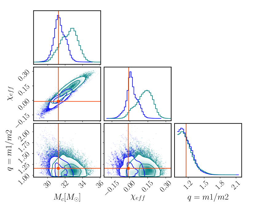
Figure 7: One-dimensional and two-dimensional posterior distributions for $M_{c}$, $q$ and $\chi_{\rm eff}$ obtained with the quasi-circular model TEOBResumS-GIOTTO (blue) and the eccentric TEOBResumS-Dalí in the quasi-circular limit (i.e. $e_{0}$ fixed to $10^{-8}$ (teal)). The solid lines indicate the values from the quasi-circular analysis presented in GWTC-1 Abbott et al. (2019).

	GW150914 Analysis
Model	TEOBResumS-GIOTTO	TEOBResumS-Dalí	TEOBResumS-Dalí	TEOBResumS-Dalí	$\rm GWTC$-$1$
$e_{0}$-prior	$e_{0}=0$(fixed)	$e_{0}=10^{-8}$ (fixed)	$\mathcal{U}$(0.001,0.2)	Log-uniform(0.001, 0.2)	–
$f_{0}$-prior	$f_{0}=$ 20 Hz (fixed)	$f_{0}=$ 20 Hz (fixed)	$\mathcal{U}$(18, 20.5)	$\mathcal{U}$(18, 20.5)	–
$M_{c}(M_{\rm\odot})$	$31.33^{+0.75}_{-0.52}$	$32.53^{+0.84}_{-1.08}$	$31.54^{+0.92}_{-1.19}$	$31.79^{+1.12}_{-0.94}$	$31.23^{+1.08}_{-0.96}$
$\chi_{\rm eff}$	$0.01^{+0.05}_{-0.03}$	$0.13^{+0.06}_{-0.08}$	$0.06^{+0.06}_{-0.10}$	$0.08^{+0.08}_{-0.07}$	$-0.01^{+0.12}_{-0.11}$
$q$	$1.14^{+0.14}_{-0.10}$	$1.15^{+0.15}_{-0.10}$	$1.18^{+0.17}_{-0.11}$	$1.21^{+0.19}_{-0.14}$	$1.16^{+0.19}_{-0.11}$
$e_{0}$	–	–	$0.05^{+0.03}_{-0.02}$	$0.02^{+0.03}_{-0.01}$	–

Table 5: Results for the different analysis of GW150914 with TEOBResumS-GIOTTO or TEOBResumS-Dalí. The prior ranges for $e_{0}$ and $f_{0}$ for each analysis are indicated. We give the median values and symmetric 90% credible interval for $M_{c}$, $\chi_{\rm eff}$ and $q$. Our results are contrasted by the values obtained from the non-eccentric, precessing analysis presented in GWTC-1 Abbott et al. (2019) shown in the last column.

V.2 Eccentric analysis of GW150914

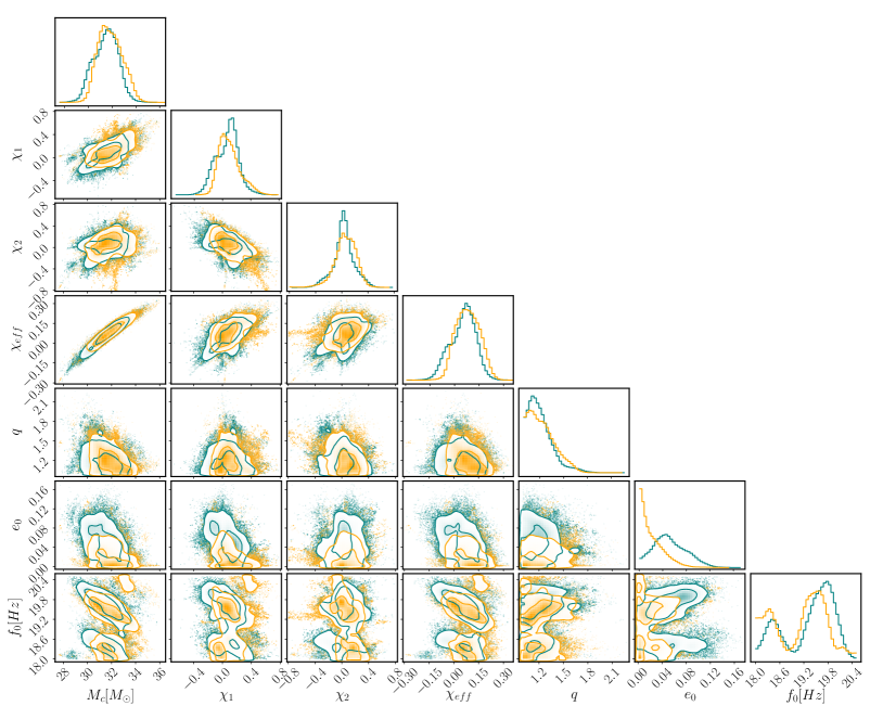
Figure 12: One dimensional and join posterior distributions for the intrinsic parameters in addition with $e_{0}$ and $f_{0}$ recovered with the two eccentric analyses of GW150914. The analysis using a uniform eccentricity prior is represented in teal, the one utilizing a logarithmic-uniform prior for the eccentricity is shown in orange.

Finally, we reanalyse GW150914 with the eccentric model TEOBResumS-Dalí sampling in both the initial eccentricity $e_{0}$ and $f_{0}$ (see Table 5 for prior details). For the eccentricity we use two different priors: one uniform in $e_{0}$ and the other one logarithmic-uniform which occupies a larger prior volume at low eccentricities. All other priors and settings are identical to the quasi-circular analysis of Sec. V.1. Consistently with this, we estimate a network SNR of $\sim 26$ with $\sim 20$ in LIGO-Hanford and $\sim 18$ in LIGO-Livingston for the maximum likelihood parameters. In Fig. 8 we show the one-dimensional and joint posterior distributions together with the median values reported in GWTC-1 Abbott et al. (2019) or calculated from PE_ (solid lines). The median values for $(M_{c},\chi_{\rm eff},q)$ are given in Table 5. The two eccentric analyses give consistent results for the mass and spin parameters, i.e. we do not find any appreciable difference between the results for the two different choices of the eccentricity prior. We do, however, find differences in the $e_{0}$ posterior under the two different prior assumptions as shown in the bottom panel of Fig. 8. While both posteriors are consistent with small values of initial eccentricity, we find that the $e_{0}$-posterior peaks at $\sim 0.05$ for the uniform $e_{0}$-prior, which is in mild tension with other results Romero-Shaw et al. (2019); Iglesias et al. (2022). However, we note that this may be due to the uniform prior, which may not sufficiently explore low values of eccentricity. By contrast, when choosing the logarithmic-uniform prior, lower values of $e_{0}$ are preferred in full agreement with other analyses. We find that the maximum 90% upper limit is $e_{0}\lesssim 0.08$, which is consistent with the results based on NR simulations presented in Abbott et al. (2017), where it was shown that the log-likelihood drops sharply as the eccentricity grows beyond $\sim 0.05$ at about $20$ Hz. For the other parameters (see Figs. 12 and 13 in Appendix C) we find broad agreement with the exception of the right ascension, where a different mode is preferred. In comparison to the quasi-circular analysis, the eccentric analyses give slightly higher median values for $M_{c}$ and $\chi_{\rm eff}$ in agreement with Romero-Shaw et al. (2019); Iglesias et al. (2022).

In terms of model selection we find that TEOBResumS-GIOTTO is favoured over TEOBResumS-Dalí with an estimated Bayes’ factor of $\ln\mathcal{B}^{\rm circ}_{\rm ecc}\sim 2$ irrespective of the prior. This is in agreement with the results reported in Romero-Shaw et al. (2019), but differs from the ones in Iglesias et al. (2022). However we note that Ref. Iglesias et al. (2022) uses higher order modes while in our analysis we only employ the dominant multipole $\ell=|m|=2$ in the waveform. We conclude that, while the hypothesis of a quasi-circular BBH merger is preferred for GW150914, we cannot exclude a small value of eccentricity at $20$ Hz. All three analyses, however, give consistent results for the intrinsic parameters at 90$\%$ confidence. Our results are in agreement with previous analyses  Abbott et al. (2019); Romero-Shaw et al. (2019, 2021).

VI Model-agnostic estimate of the Eccentricity Evolution

Bayesian inference allows us to determine the posterior distributions of binary parameters at a certain reference frequency. Certain parameters are, however, frequency dependent and hence change over time. One of these parameters is the eccentricity of the orbit, which decays due to the emission of GWs. In Sec. V.2 we determined the posterior distribution of the initial eccentricity $e_{0}$ of the EOB model measured at a (varying) reference average frequency $f_{0}$. We now devise a scheme to determine the evolution of the eccentricity as a function of frequency using a previously introduced eccentricity estimator Mora and Will (2002). Gravitational radiation at future null infinity is expected to be manifestly gauge invariant, motivating the use of an estimator based on the relative oscillations in the gravitational-wave frequency. This mitigates against the contamination of eccentricity measurements through the use of gauge dependent quantities Mora and Will (2004). This has the additional advantage of allowing for the direct comparison between different eccentric analyses, which often use different definitions of eccentricity M. Knee et al. (2022). Our scheme is computationally efficient and applicable to any eccentric waveform model in post-processing. A benefit of this way of estimating the eccentricity in post-processing is that it can be calculated directly from the GW signal in contrast to definitions inferred from the dynamics . In addition, it also reduces to the Newtonian definition of eccentricity, even in the high eccentricity limit  Mora and Will (2002); Ramos-Buades et al. (2020).

To calculate the eccentricity evolution, we employ the eccentricity estimator first introduced by Mora et al. Mora and Will (2002):

$$e_{\omega}(t)=\frac{\omega_{p}(t)^{1/2}-\omega_{a}(t)^{1/2}}{\omega_{p}(t)^{1/2}+\omega_{a}(t)^{1/2}},$$ (17)

where $\omega_{p}(t)$ and $\omega_{a}(t)$ are fits to the GW frequency of the $(2,2)$-mode at the periastron and the apastron, respectively. We note that this eccentricity estimator is also used in other works, e.g. either based on the orbital Lewis et al. (2017); Ramos-Buades et al. (2020); Islam et al. (2021) or the GW frequency Chiaramello and Nagar (2020); Nagar et al. (2021).

To calculate $\omega_{p}(t)$ and $\omega_{a}(t)$, we first generate the TEOBResumS-Dalí waveform for each posterior sample and compute the GW frequency as $\omega(t)=\dot{\phi}(t)$, where $\phi(t)$ is the phase of the $(2,2)$-mode defined as $h_{22}=A(t)e^{-i\phi(t)}$ with $A(t)$ being the amplitude of the waveform. We then identify the maxima (periastron) and the minima (apastron) of the second time-derivative of the GW frequency. We use the second derivative in order to amplify the peaks such that the identification of the maxima and minima is more robust for small eccentricities.

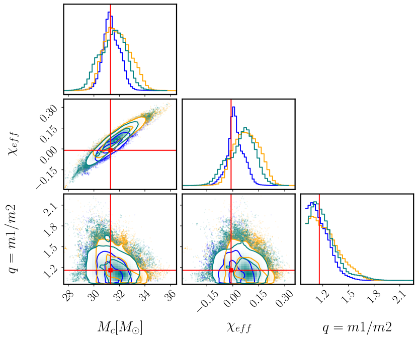
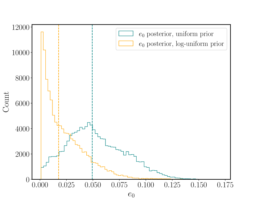
Figure 8: Analyses of GW150914 with TEOBResumS-GIOTTO (blue) and TEOBResumS-Dalí with a uniform $e_{0}$-prior (teal) and a logarithmic-uniform $e_{0}$-prior (orange). Upper panel: Joint posterior distributions with 90$\%$ and 50$\%$ credibility interval and median values reported in GWTC-1  Abbott et al. (2019) (solid lines). Bottom panel: Marginalised one-dimensional posterior distributions and median values of $e_{0}$ (dashed lines) for the two eccentric analyses.

Figure 9: Upper panel: Illustration of the fitting procedure to determine the maxima (teal) and minima (orange) of the GW frequency (red). Bottom panel: Evolution of the eccentricity $e_{\omega}(t)$ calculated using the method described in the text for a BBH with $M_{c}=24.74$, $\chi_{\rm eff}=0$ and $q=1.5$.

Once the minima and maxima are identified, we fit $f(t)=\omega(t)/(2\pi)$ using cubic spline interpolation. An example of this is shown in the upper panel of Fig. 9, where the red curve shows the GW frequency with clearly visible eccentricity-induced oscillations and the green and orange curves show the fits to the maxima and minima respectively. From Eq. (17) we calculate $e_{\omega}(t)$ for each posterior sample to find the corresponding eccentricity evolution, as shown in the bottom panel of Fig. 9. We note that the eccentricity estimated at the initial time $e_{\omega}(t=0)$ can differ from the initial EOB eccentricity $e_{0}$ defined by the EOB dynamics as the eccentricity at the average frequency between apastron and periastron, as explained by Eq. (21).

Since we are interested in determining how the eccentricity decays as the GW frequency increases towards merger, we need to map $t\rightarrow f$. Due to the non-monotonic behavior of the GW frequency, such a mapping is not unique and hence we introduce the average GW frequency $\bar{f}(t)$ instead:

$$\bar{f}(t)=\frac{1}{2}\left(f_{p}(t)+f_{a}(t)\right),$$ (18)

where $f_{p}(t)=\omega_{p}(t)/(2\pi)$ and $f_{a}(t)=\omega_{a}(t)/(2\pi)$, and use linear interpolation to infer the eccentricity as a function of $\bar{f}$ throughout the inspiral.

As we mentioned before, this method benefits of the fact that it allows the eccentricity to be calculated directly from the GW signal and it reduces to the Newtonian definition of eccentricity, even in the high eccentricity limit, however, the method also has some limitations. A caveat to the correct calculation of $e_{\omega}(t)$ is, in fact, that it requires the inspiral to be sufficiently long such that many periastron and apastron peaks can be resolved. In particular, for short waveforms where we only have one or two maxima and minima available, this method is expected to become inefficient and inaccurate Ramos-Buades et al. (2020). A way to circumvent this situation is to generate the EOB waveforms from a lower starting frequency but at the cost of increasing the waveform generation time and hence the time taken for a Bayesian inference run to complete. Similarly, in the low-eccentricity limit, we may also expect peak-finding algorithms to become numerically unstable. While strategies to amplify the peaks, such as the use of the second derivative of the frequency, help to isolate the stationary points, in practice we found that the peaks can still be poorly resolved for a small subset of the samples. However, by cutting the frequencies at sufficiently small times ($t=0.4$ s), we found the eccentricity estimator to be numerically robust with only a small percentage of samples $(\lesssim 0.03\%)$ potentially suffering from pathologies. For those samples, we can adjust the cutoff time/frequency to produce an estimate of the eccentricity.

In Fig. 10 we show the 90% upper limit of the eccentricity evolution $e_{\omega}(\bar{f})$ as a function of the average frequency for the simulated eccentric signal with $e_{0}=0.05$ and $f_{0}=20$Hz, as discussed in Sec. IV.2. In addition, we also show the eccentricity evolution for the injected waveform itself (black triangles). We see that it is always contained within the $90\%$ upper limit.

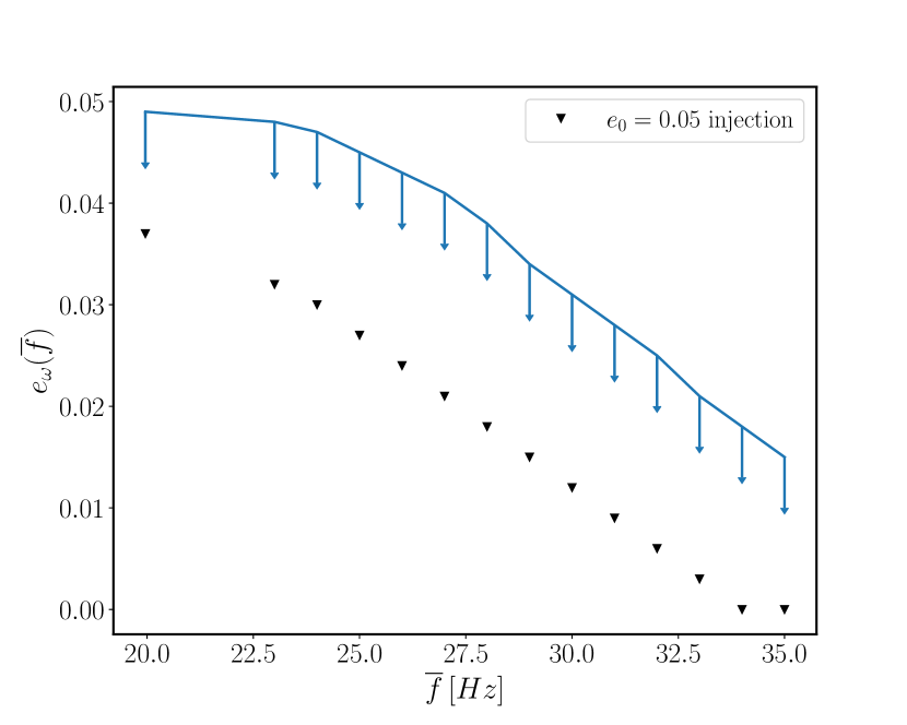
Figure 10: Upper limit of the 90$\%$ credibility interval for the estimated eccentricity evolution $e_{\omega}(\bar{f})$ for an injection with $e_{0}=0.05$. The upper limit is calculated estimating $e_{\omega}(\bar{f})$ for all the posterior samples, interpolating it at different values of $\bar{f}$ and then taking the 90 $\%$ credibility interval of the of the data. The black triangles represent the injection. We note that the estimated initial eccentricity is slightly lower than $e_{0}=0.05$, where $e_{0}$ is defined from the EOB dynamics.

Finally, we apply the same method to calculate the eccentricity evolution for GW150914 from the posterior samples obtained using the eccentric TEOBResumS-Dalí model as outlined in Sec. V.2. Figure 11 shows the $90\%$ upper limit of $e_{\omega}(\bar{f})$ obtained for the uniform $e_{0}$-prior distribution (blue) as well as for the log-uniform $e_{0}$-prior distribution (orange). We obtain an upper limit of $e_{\omega}(\bar{f})$ at $\sim$ 20 Hz of $\sim 0.075$ for the analysis with the uniform $e_{0}$-prior and $\sim 0.055$ for the analysis with the logarithmic-uniform $e_{0}$-prior. This is comparable with Fig. 7 of Abbott et al. (2017) where it was found that GW150914 is unlikely to have an eccentricity higher than $\sim$ 0.05 at about 20 Hz at $90\%$ credibility. We also see that while we cannot exclude small values of eccentricities at low frequencies, once an average frequency of $\sim 30$ Hz is reached, any residual eccentricity $e_{\omega}(\bar{f})$ can no longer be distinguished from zero.

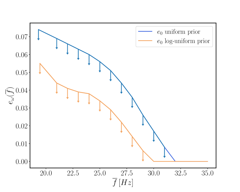
Figure 11: Upper limit of the 90$\%$ credibility interval for the estimated eccentricity evolution $e_{\omega}(\bar{f})$ for the two eccentric analyses of GW150914 with TEOBResumS-Dalí. The upper limit is calculated estimating $e_{\omega}(\bar{f})$ for all the posterior samples, interpolating it at different values of $\bar{f}$ and then taking the 90 $\%$ credible interval of the data. This result is agreement with previous results Abbott et al. (2017).

VII Discussion

In this work we present a Bayesian validation of the TEOBResumS-Dalí waveform model Nagar et al. (2021) for eccentric coalescing binary black holes with aligned spins, a fully Bayesian reanalysis of GW150914 and a systematic method to estimate the eccentricity in post-processing. Our study explores the potential of TEOBResumS-Dalí and allows us to test its reliability. Our work is an extension of our previous study Nagar et al. (2021) and demonstrates the efficacy of the model in distinguishing between circular and eccentric GW signals. In particular, we find that the differences between the quasi-circular limit of TEOBResumS-Dalí and its quasi-circular companion TEOBResumS-GIOTTO are relevant, and lead to clear (though small) biases in the recovered parameters. We attribute these biases to differences between the two models in both the dynamics (and especially in the radiative sector) and the waveform itself. When performing parameter estimation with small fixed eccentricity this results in appreciable differences in the posteriors of numerous parameters. This indicates that the original TEOBResumS-Dalí model needs improvements, notably to recover a quasi-circular limit that is as accurate as the one of TEOBResumS-GIOTTO. Some work in this direction has been done Nagar and Rettegno (2021) (see in particular Fig. 8 therein) but more investigations are needed to improve the model in the nearly equal-mass regime.

After testing TEOBResumS-Dalí for quasi-circular binaries, we validate the model on injections with nonzero initial eccentricity. In particular we find that TEOBResumS-Dalí excellently recovers the injected value of eccentricity. In addition, we quantify the impact of eccentricity on the estimation of the intrinsic parameters of the binary: notably, we observe that the correlations between parameters became less strong when introducing eccentricity. If neglecting eccentricity, however, we see biases in the mass and spin parameters to compensate for it.

We then perform Bayesian inference with TEOBResumS-Dalí on the first GW event, GW150914. We find that the circular analysis is preferred with respect to the eccentric ones with $\ln\mathcal{B}^{\rm circ}_{\rm ecc}\sim 2$. However, we also find that we cannot exclude small values of eccentricities at low frequencies, and that once an average frequency of $\sim 30$ Hz is reached, any residual eccentricity becomes indistinguishable from zero.

Lastly we perform the calculation of the eccentricity evolution using an eccentricity estimator deduced from the instantaneous GW frequency. After testing the calculation on mock signals, we apply the method to the data of GW150914 finding that, at about 20 Hz, the maximum eccentricity allows for the system is $\sim 0.075$ for a uniform prior and $\sim 0.055$ for a logarithmic-uniform prior on the initial eccentricity. This is quantitatively comparable with the findings of Abbott et al. (2017). In the late stages of the preparation of this manuscript we became aware of related but independent work on eccentricity definitions Shaikh et al. (2022).

Given current BBH merger rate estimates Abbott et al. (2021) and the sensitivity of the LIGO-Virgo-KAGRA detector network LVK , future detections of eccentric binaries will significantly constrain the lower limit of mergers that result from clusters and other dynamical channels Zevin et al. (2021). The possibility of several eccentric BBH candidates Romero-Shaw et al. (2022); Iglesias et al. (2022) makes it crucial to have a reliable method to infer the eccentricity directly from observations. For the first time we present a systematic method to infer the eccentricity evolution directly from observations of GWs from coalescing BBHs that can be used in the future to robustly measure the eccentricity and make meaningful comparisons between different models.

Appendix A Quasi-circular and eccentric initial conditions

For quasi-circular binaries, TEOBResumS applies Kepler’s law to the initial frequency of the orbit to compute the initial separation $r$. Then, the initial values of the EOB angular and radial momenta $p_{\varphi},p_{r_{*}}$ are estimated via an iterative process (known as post-adiabatic expansion, “PA” henceforth) in which the right-hand side of the Hamilton equations is solved analytically under the assumption that $p_{r_{*}}\sim 0$ Damour et al. (2013); Nagar and Rettegno (2019). At zeroth PA order, one assumes that $p_{r_{*}}=0$ exactly. Then, by evaluating $\partial_{r}\hat{H}_{\rm EOB}=0$ one can analytically find the circular angular momentum $j_{0}(r)$ at the requested initial separation. Neglecting terms of $O(p_{r_{*}}^{2})$, one can then use $dp_{\varphi}/dr=\hat{\mathcal{F}}_{\varphi}\dot{r}^{-1}$ to compute $p_{r_{*}}$ at the first PA order. This procedure can then be repeated any number of times, with even (odd) PA orders providing corrections to $p_{\varphi}$ ($p_{r_{*}}$). Correctly computing the initial conditions of the systems and having $p_{r_{*}}$ different from zero at the initial separation is crucial to avoid effects due to spurious eccentricity.

For eccentric binaries, initial conditions necessarily need to be specified in a different manner. Let us denote with $e$ the eccentricity of the ellipse that the system would orbit along assuming no GW emission. Similarly, let us denote with $p$ its semilatus rectum and with $\xi$ its anomaly. A generic point on the ellipse has radial coordinate $r=p/(1+e\cos\xi)$. To find adiabatic initial conditions for our EOB dynamics we need to find a way to map $(f_{0},e,\xi)$ into $(r_{0},p_{\varphi}^{0},p_{r_{*}}^{0})$. In practice, for convenience, the initial orbital frequency $\Omega_{0}$ is always assumed to correspond either to the apastron ($r_{0}=p_{0}/(1-e)$), periastron ($r_{0}=p_{0}/(1+e)$) or to the average frequency between the two points. We then solve numerically

$$\partial_{p_{\varphi}}H(r_{0}(p_{0}),j_{0}(p_{0}),p_{r_{*}}=0)=\Omega_{0}$$ (19)

where $j_{0}$ is the adiabatic angular momentum computed using energy conservation

$$\hat{H}_{\rm eff}^{0}(p_{0},j_{0},\xi=0)=\hat{H}_{\rm eff}^{0}(p_{0},j_{0},\xi=\pi),$$ (20)

and estimate the semilatus rectum of the obit $p_{0}$. The evolution of the system is then always started at the apastron, so that

$$r_{0} =\frac{p_{0}}{(1-e)},$$ (21)

$$p_{\varphi}^{0} =j_{0},$$ (22)

$$p_{r_{*}}^{0} =0.$$ (23)

This adiabatic procedure can be generalized to higher PA orders. We leave a discussion of such initial conditions to future work.

Appendix B Tables

In this section we report the posteriors for $M_{c}$, $\chi_{\rm eff}$ and $q$ for two injections and different recoveries performed.

	Circular injection
Model	TEOBResumS-GIOTTO	TEOBResumS-Dalí	TEOBResumS-Dalí	TEOBResumS-Dalí	TEOBResumS-Dalí
$e_{0}$-prior	$e_{0}=0$ (fixed)	$e_{0}=10^{-8}$ (fixed)	$\mathcal{U}$(0.001,0.2)	$\mathcal{U}$(0.001,0.2)	Log-uniform(0.001, 0.2)
$f_{0}$-prior	$f_{0}=$ 20 Hz (fixed)	$f_{0}=$ 20 Hz (fixed)	$\mathcal{U}$(18, 20.5)	$f_{0}=$ 20 Hz	$\mathcal{U}$(18, 20.5)
$M_{c}(M_{\rm\odot})$	$24.38_{-0.16}^{+0.17}$	$24.53_{-0.17}^{+0.18}$	$24.32_{-0.19}^{+0.18}$	$24.33_{-0.21}^{+0.18}$	$24.35_{-0.16}^{+0.17}$
$\chi_{\rm eff}$	$0.01_{-0.03}^{0.03}$	$0.04_{-0.03}^{+0.03}$	$0.00_{-0.03}^{+0.03}$	$0.00_{-0.03}^{+0.03}$	$0.00_{-0.02}^{+0.02}$
$q$	$2.00_{-0.19}^{+0.22}$	$2.08_{-0.20}^{+0.18}$	$2.00_{-0.19}^{+0.14}$	$2.02_{-0.18}^{+0.17}$	$1.97_{-0.20}^{+0.17}$
$e_{0}$	–	–	$0.01_{-0.01}^{+0.01}$	$0.01_{-0.01}^{+0.01}$	$0.00_{-0.01}^{+0.01}$

Table 6: Posterior distribution functions for $M_{c}$, $\chi_{\rm eff}$ and $q$ for a circular injection ($e^{\rm inj}_{\omega}=0$ and $f_{0}=20$Hz) with different recoveries using TEOBResumS-GIOTTO and TEOBResumS-Dalí.

	Eccentric injection
Model	TEOBResumS-GIOTTO	TEOBResumS-Dalí
$e_{0}$-prior	$e_{0}=0$ (fixed)	$\mathcal{U}$(0.001,0.2)
$f_{0}$-prior	$f_{0}=$ 20 Hz (fixed)	$\mathcal{U}$(18, 20.5)
$M_{c}(M_{\rm\odot})$	$24.34_{-0.17}^{+0.17}$	$24.43_{-0.24}^{+0.19}$
$\chi_{\rm eff}$	$-0.03_{-0.03}^{+0.03}$	$-0.03_{-0.03}^{+0.03}$
$q$	$1.84_{-0.21}^{+0.19}$	$1.97_{-0.20}^{+0.17}$
$e_{0}$	–	$0.05_{-0.01}^{+0.01}$

Table 7: Posterior distribution functions for $M_{c}$, $\chi_{\rm eff}$ and $q$ for an eccentric injection ($e^{\rm inj}_{\omega}=0.05$ and $f_{0}=20$Hz) with different recoveries using TEOBResumS-GIOTTO and TEOBResumS-Dalí.

Appendix C Full corner plots for the GW150914 eccentric analysis

In this section we report the full corner plots showing the posterior distributions of the intrinsic and extrinsic parameters relative to the eccentric analysis of GW150914.

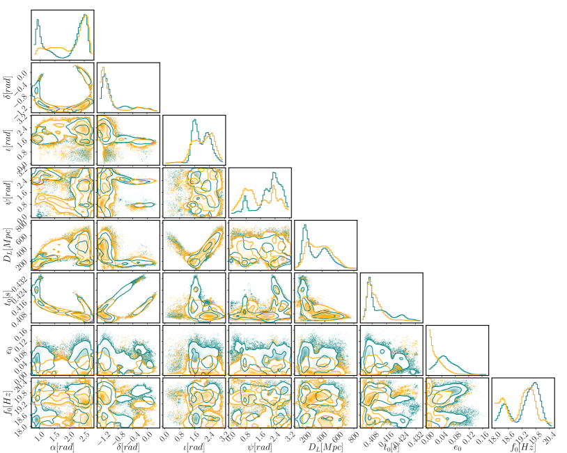
Figure 13: One dimensional and join posterior distributions for the extrinsic parameters in addition with $e_{0}$ and $f_{0}$ recovered with the two eccentric analyses of GW150914. The analysis using a uniform eccentricity prior is represented in teal, the one utilizing a logarithmic-uniform prior for the eccentricity is shown in orange.

References

- Peters and Mathews (1963) P. C. Peters and J. Mathews, “Gravitational radiation from point masses in a Keplerian orbit,” Phys. Rev. 131, 435–439 (1963).
- Samsing (2018) Johan Samsing, “Eccentric Black Hole Mergers Forming in Globular Clusters,” Phys. Rev. D97, 103014 (2018), arXiv:1711.07452 [astro-ph.HE] .
- Rodriguez et al. (2018) Carl L. Rodriguez, Pau Amaro-Seoane, Sourav Chatterjee, and Frederic A. Rasio, “Post-Newtonian Dynamics in Dense Star Clusters: Highly-Eccentric, Highly-Spinning, and Repeated Binary Black Hole Mergers,” Phys. Rev. Lett. 120, 151101 (2018), arXiv:1712.04937 [astro-ph.HE] .
- Fragione et al. (2019) Giacomo Fragione, Evgeni Grishin, Nathan W. C. Leigh, Hagai. B. Perets, and Rosalba Perna, “Black hole and neutron star mergers in galactic nuclei,” Mon. Not. Roy. Astron. Soc. 488, 47–63 (2019), arXiv:1811.10627 [astro-ph.GA] .
- Samsing et al. (2020) J. Samsing, I. Bartos, D. J. D’Orazio, Z. Haiman, B. Kocsis, N. W. C. Leigh, B. Liu, M. E. Pessah, and H. Tagawa, “Active Galactic Nuclei as Factories for Eccentric Black Hole Mergers,” (2020), arXiv:2010.09765 [astro-ph.HE] .
- Zevin et al. (2021) Michael Zevin, Isobel M. Romero-Shaw, Kyle Kremer, Eric Thrane, and Paul D. Lasky, “Implications of Eccentric Observations on Binary Black Hole Formation Channels,” Astrophys. J. Lett. 921, L43 (2021), arXiv:2106.09042 [astro-ph.HE] .
- Tagawa et al. (2021) Hiromichi Tagawa, Bence Kocsis, Zoltan Haiman, Imre Bartos, Kazuyuki Omukai, and Johan Samsing, “Eccentric Black Hole Mergers in Active Galactic Nuclei,” Astrophys. J. Lett. 907, L20 (2021), arXiv:2010.10526 [astro-ph.HE] .
- Gayathri et al. (2022) V. Gayathri, J. Healy, J. Lange, B. O’Brien, M. Szczepanczyk, Imre Bartos, M. Campanelli, S. Klimenko, C. O. Lousto, and R. O’Shaughnessy, “Eccentricity estimate for black hole mergers with numerical relativity simulations,” Nature Astron. 6, 344–349 (2022), arXiv:2009.05461 [astro-ph.HE] .
- Romero-Shaw et al. (2022) Isobel M. Romero-Shaw, Paul D. Lasky, and Eric Thrane, “Four eccentric mergers increase the evidence that LIGO–Virgo–KAGRA’s binary black holes form dynamically,” (2022), arXiv:2206.14695 [astro-ph.HE] .
- Clarke et al. (2022) Teagan A. Clarke, Isobel M. Romero-Shaw, Paul D. Lasky, and Eric Thrane, “Gravitational-wave inference for eccentric binaries: the argument of periapsis,” (2022), arXiv:2206.14006 [gr-qc] .
- Romero-Shaw et al. (2021) Isobel M. Romero-Shaw, Paul D. Lasky, and Eric Thrane, “Signs of Eccentricity in Two Gravitational-wave Signals May Indicate a Subpopulation of Dynamically Assembled Binary Black Holes,” Astrophys. J. Lett. 921, L31 (2021), arXiv:2108.01284 [astro-ph.HE] .
- Abbott et al. (2020) R. Abbott et al. (LIGO Scientific, Virgo), “GW190521: A Binary Black Hole Merger with a Total Mass of ,” Phys. Rev. Lett. 125, 101102 (2020), arXiv:2009.01075 [gr-qc] .
- Gamba et al. (2021) Rossella Gamba, Matteo Breschi, Gregorio Carullo, Piero Rettegno, Simone Albanesi, Sebastiano Bernuzzi, and Alessandro Nagar, “GW190521: A dynamical capture of two black holes,” Submitted to Nature Astronomy (2021), arXiv:2106.05575 [gr-qc] .
- Romero-Shaw et al. (2020) Isobel M. Romero-Shaw, Paul D. Lasky, Eric Thrane, and Juan Calderon Bustillo, “GW190521: orbital eccentricity and signatures of dynamical formation in a binary black hole merger signal,” Astrophys. J. Lett. 903, L5 (2020), arXiv:2009.04771 [astro-ph.HE] .
- Bustillo et al. (2021) Juan Calderón Bustillo, Nicolas Sanchis-Gual, Alejandro Torres-Forné, José A. Font, Avi Vajpeyi, Rory Smith, Carlos Herdeiro, Eugen Radu, and Samson H. W. Leong, “GW190521 as a Merger of Proca Stars: A Potential New Vector Boson of eV,” Phys. Rev. Lett. 126, 081101 (2021), arXiv:2009.05376 [gr-qc] .
- Buonanno and Damour (1999) A. Buonanno and T. Damour, “Effective one-body approach to general relativistic two-body dynamics,” Phys. Rev. D59, 084006 (1999), arXiv:gr-qc/9811091 .
- Buonanno and Damour (2000) Alessandra Buonanno and Thibault Damour, “Transition from inspiral to plunge in binary black hole coalescences,” Phys. Rev. D62, 064015 (2000), arXiv:gr-qc/0001013 .
- Damour et al. (2000) Thibault Damour, Piotr Jaranowski, and Gerhard Schaefer, “On the determination of the last stable orbit for circular general relativistic binaries at the third postNewtonian approximation,” Phys. Rev. D62, 084011 (2000), arXiv:gr-qc/0005034 [gr-qc] .
- Damour (2001) Thibault Damour, “Coalescence of two spinning black holes: An effective one- body approach,” Phys. Rev. D64, 124013 (2001), arXiv:gr-qc/0103018 .
- Hinderer and Babak (2017) Tanja Hinderer and Stanislav Babak, “Foundations of an effective-one-body model for coalescing binaries on eccentric orbits,” Phys. Rev. D96, 104048 (2017), arXiv:1707.08426 [gr-qc] .
- Cao and Han (2017) Zhoujian Cao and Wen-Biao Han, “Waveform model for an eccentric binary black hole based on the effective-one-body-numerical-relativity formalism,” Phys. Rev. D96, 044028 (2017), arXiv:1708.00166 [gr-qc] .
- Liu et al. (2019) Xiaolin Liu, Zhoujian Cao, and Lijing Shao, “Validating the Effective-One-Body Numerical-Relativity Waveform Models for Spin-aligned Binary Black Holes along Eccentric Orbits,” (2019), arXiv:1910.00784 [gr-qc] .
- Chiaramello and Nagar (2020) Danilo Chiaramello and Alessandro Nagar, “Faithful analytical effective-one-body waveform model for spin-aligned, moderately eccentric, coalescing black hole binaries,” Phys. Rev. D 101, 101501 (2020), arXiv:2001.11736 [gr-qc] .
- Nagar et al. (2021) Alessandro Nagar, Alice Bonino, and Piero Rettegno, “Effective one-body multipolar waveform model for spin-aligned, quasicircular, eccentric, hyperbolic black hole binaries,” Phys. Rev. D 103, 104021 (2021), arXiv:2101.08624 [gr-qc] .
- Placidi et al. (2021) Andrea Placidi, Simone Albanesi, Alessandro Nagar, Marta Orselli, Sebastiano Bernuzzi, and Gianluca Grignani, “Exploiting Newton-factorized, 2PN-accurate, waveform multipoles in effective-one-body models for spin-aligned noncircularized binaries,” (2021), arXiv:2112.05448 [gr-qc] .
- Albertini et al. (2021) Angelica Albertini, Alessandro Nagar, Piero Rettegno, Simone Albanesi, and Rossella Gamba, “Waveforms and fluxes: Towards a self-consistent effective one body waveform model for nonprecessing, coalescing black-hole binaries for third generation detectors,” (2021), arXiv:2111.14149 [gr-qc] .
- Albanesi et al. (2022a) Simone Albanesi, Alessandro Nagar, Sebastiano Bernuzzi, Andrea Placidi, and Marta Orselli, “Assessment of Effective-One-Body Radiation Reactions for Generic Planar Orbits,” (2022a), arXiv:2202.10063 [gr-qc] .
- Albanesi et al. (2022b) Simone Albanesi, Andrea Placidi, Alessandro Nagar, Marta Orselli, and Sebastiano Bernuzzi, “New avenue for accurate analytical waveforms and fluxes for eccentric compact binaries,” Phys. Rev. D 105, L121503 (2022b), arXiv:2203.16286 [gr-qc] .
- Ramos-Buades et al. (2022) Antoni Ramos-Buades, Alessandra Buonanno, Mohammed Khalil, and Serguei Ossokine, “Effective-one-body multipolar waveforms for eccentric binary black holes with nonprecessing spins,” Phys. Rev. D 105, 044035 (2022), arXiv:2112.06952 [gr-qc] .
- Liu et al. (2021) Xiaolin Liu, Zhoujian Cao, and Zong-Hong Zhu, “A higher-multipole gravitational waveform model for an eccentric binary black holes based on the effective-one-body-numerical-relativity formalism,” (2021), arXiv:2102.08614 [gr-qc] .
- Yun et al. (2021) Qianyun Yun, Wen-Biao Han, Xingyu Zhong, and Carlos A. Benavides-Gallego, “Surrogate model for gravitational waveforms of spin-aligned binary black holes with eccentricities,” Phys. Rev. D 103, 124053 (2021), arXiv:2104.03789 [gr-qc] .
- Islam et al. (2021) Tousif Islam, Vijay Varma, Jackie Lodman, Scott E. Field, Gaurav Khanna, Mark A. Scheel, Harald P. Pfeiffer, Davide Gerosa, and Lawrence E. Kidder, “Eccentric binary black hole surrogate models for the gravitational waveform and remnant properties: comparable mass, nonspinning case,” (2021), arXiv:2101.11798 [gr-qc] .
- Huerta et al. (2018) E. A. Huerta et al., “Eccentric, nonspinning, inspiral, Gaussian-process merger approximant for the detection and characterization of eccentric binary black hole mergers,” Phys. Rev. D97, 024031 (2018), arXiv:1711.06276 [gr-qc] .
- Ramos-Buades et al. (2020) Antoni Ramos-Buades, Sascha Husa, Geraint Pratten, Héctor Estellés, Cecilio García-Quirós, Maite Mateu-Lucena, Marta Colleoni, and Rafel Jaume, “First survey of spinning eccentric black hole mergers: Numerical relativity simulations, hybrid waveforms, and parameter estimation,” Phys. Rev. D 101, 083015 (2020), arXiv:1909.11011 [gr-qc] .
- Tiwari and Gopakumar (2020) Srishti Tiwari and Achamveedu Gopakumar, “Combining post-circular and Padé approximations to compute Fourier domain templates for eccentric inspirals,” Phys. Rev. D 102, 084042 (2020), arXiv:2009.11333 [gr-qc] .
- Cho et al. (2021) Gihyuk Cho, Sashwat Tanay, Achamveedu Gopakumar, and Hyung Mok Lee, “Generalized quasi-Keplerian solution for eccentric, non-spinning compact binaries at 4PN order and the associated IMR waveform,” (2021), arXiv:2110.09608 [gr-qc] .
- Chattaraj et al. (2022) Abhishek Chattaraj, Tamal RoyChowdhury, Divyajyoti, Chandra Kant Mishra, and Anshu Gupta, “High accuracy PN and NR comparisons involving higher modes for eccentric BBHs and a dominant mode eccentric IMR model,” (2022), arXiv:2204.02377 [gr-qc] .
- Loutrel and Yunes (2017) Nicholas Loutrel and Nicolas Yunes, “Hereditary Effects in Eccentric Compact Binary Inspirals to Third Post-Newtonian Order,” Class. Quant. Grav. 34, 044003 (2017), arXiv:1607.05409 [gr-qc] .
- Loutrel et al. (2019) Nicholas Loutrel, Samuel Liebersbach, Nicolás Yunes, and Neil Cornish, “The eccentric behavior of inspiralling compact binaries,” Class. Quant. Grav. 36, 025004 (2019), arXiv:1810.03521 [gr-qc] .
- Moore and Yunes (2019) Blake Moore and Nicolás Yunes, “A 3PN Fourier Domain Waveform for Non-Spinning Binaries with Moderate Eccentricity,” Class. Quant. Grav. 36, 185003 (2019), arXiv:1903.05203 [gr-qc] .
- Boetzel et al. (2019) Yannick Boetzel, Chandra Kant Mishra, Guillaume Faye, Achamveedu Gopakumar, and Bala R. Iyer, “Gravitational-wave amplitudes for compact binaries in eccentric orbits at the third post-Newtonian order: Tail contributions and postadiabatic corrections,” Phys. Rev. D 100, 044018 (2019), arXiv:1904.11814 [gr-qc] .
- Klein (2021) Antoine Klein, “EFPE: Efficient fully precessing eccentric gravitational waveforms for binaries with long inspirals,” (2021), arXiv:2106.10291 [gr-qc] .
- Tucker and Will (2021) Alexandria Tucker and Clifford M. Will, “Residual eccentricity of inspiralling orbits at the gravitational-wave detection threshold: Accurate estimates using post-Newtonian theory,” Phys. Rev. D 104, 104023 (2021), arXiv:2108.12210 [gr-qc] .
- Nagar et al. (2018) Alessandro Nagar et al., “Time-domain effective-one-body gravitational waveforms for coalescing compact binaries with nonprecessing spins, tides and self-spin effects,” Phys. Rev. D98, 104052 (2018), arXiv:1806.01772 [gr-qc] .
- Nagar et al. (2020) Alessandro Nagar, Gunnar Riemenschneider, Geraint Pratten, Piero Rettegno, and Francesco Messina, “Multipolar effective one body waveform model for spin-aligned black hole binaries,” Phys. Rev. D 102, 024077 (2020), arXiv:2001.09082 [gr-qc] .
- Riemenschneider et al. (2021) Gunnar Riemenschneider, Piero Rettegno, Matteo Breschi, Angelica Albertini, Rossella Gamba, Sebastiano Bernuzzi, and Alessandro Nagar, “Assessment of consistent next-to-quasicircular corrections and postadiabatic approximation in effective-one-body multipolar waveforms for binary black hole coalescences,” Phys. Rev. D 104, 104045 (2021), arXiv:2104.07533 [gr-qc] .
- Nagar and Rettegno (2021) Alessandro Nagar and Piero Rettegno, “The next generation: Impact of high-order analytical information on effective one body waveform models for noncircularized, spin-aligned black hole binaries,” (2021), arXiv:2108.02043 [gr-qc] .
- Khalil et al. (2021) Mohammed Khalil, Alessandra Buonanno, Jan Steinhoff, and Justin Vines, “Radiation-reaction force and multipolar waveforms for eccentric, spin-aligned binaries in the effective-one-body formalism,” Phys. Rev. D 104, 024046 (2021), arXiv:2104.11705 [gr-qc] .
- Damour and Nagar (2014) Thibault Damour and Alessandro Nagar, “New effective-one-body description of coalescing nonprecessing spinning black-hole binaries,” Phys.Rev. D90, 044018 (2014), arXiv:1406.6913 [gr-qc] .
- Nagar et al. (2016) Alessandro Nagar, Thibault Damour, Christian Reisswig, and Denis Pollney, “Energetics and phasing of nonprecessing spinning coalescing black hole binaries,” Phys. Rev. D93, 044046 (2016), arXiv:1506.08457 [gr-qc] .
- Nagar et al. (2019) Alessandro Nagar, Geraint Pratten, Gunnar Riemenschneider, and Rossella Gamba, “A Multipolar Effective One Body Model for Non-Spinning Black Hole Binaries,” (2019), arXiv:1904.09550 [gr-qc] .
- (52) “SXS Gravitational Waveform Database,” https://data.black-holes.org/waveforms/index.html.
- Damour et al. (2013) Thibault Damour, Alessandro Nagar, and Sebastiano Bernuzzi, “Improved effective-one-body description of coalescing nonspinning black-hole binaries and its numerical-relativity completion,” Phys.Rev. D87, 084035 (2013), arXiv:1212.4357 [gr-qc] .
- Albanesi et al. (2021) Simone Albanesi, Alessandro Nagar, and Sebastiano Bernuzzi, “Effective one-body model for extreme-mass-ratio spinning binaries on eccentric equatorial orbits: Testing radiation reaction and waveform,” Phys. Rev. D 104, 024067 (2021), arXiv:2104.10559 [gr-qc] .
- Boyle et al. (2019) Michael Boyle et al., “The SXS Collaboration catalog of binary black hole simulations,” Class. Quant. Grav. 36, 195006 (2019), arXiv:1904.04831 [gr-qc] .
- Buikema et al. (2020) Aaron Buikema et al. (aLIGO), “Sensitivity and performance of the Advanced LIGO detectors in the third observing run,” Phys. Rev. D 102, 062003 (2020), arXiv:2008.01301 [astro-ph.IM] .
- Bayes (1764) Thomas Bayes, Rev., “An essay toward solving a problem in the doctrine of chances,” Phil. Trans. Roy. Soc. Lond. 53, 370–418 (1764).
- Breschi et al. (2021) Matteo Breschi, Rossella Gamba, and Sebastiano Bernuzzi, “Bayesian inference of multimessenger astrophysical data: Methods and applications to gravitational waves,” Phys. Rev. D 104, 042001 (2021), arXiv:2102.00017 [gr-qc] .
- Skilling (2006) John Skilling, “Nested sampling for general bayesian computation,” Bayesian Anal. 1, 833–859 (2006).
- Speagle (2020) Joshua S Speagle, “dynesty: a dynamic nested sampling package for estimating bayesian posteriors and evidences,” Monthly Notices of the Royal Astronomical Society 493, 3132?3158 (2020).
- Abbott et al. (2019) B. P. Abbott et al. (LIGO Scientific, Virgo), “GWTC-1: A Gravitational-Wave Transient Catalog of Compact Binary Mergers Observed by LIGO and Virgo during the First and Second Observing Runs,” Phys. Rev. X9, 031040 (2019), arXiv:1811.12907 [astro-ph.HE] .
- Lange et al. (2018) Jacob Lange, Richard O’Shaughnessy, and Monica Rizzo, “Rapid and accurate parameter inference for coalescing, precessing compact binaries,” (2018), arXiv:1805.10457 [gr-qc] .
- Abbott et al. (2016) Benjamin P. Abbott et al., “Sensitivity of the Advanced LIGO detectors at the beginning of gravitational wave astronomy,” Phys. Rev. D 93, 112004 (2016), [Addendum: Phys.Rev.D 97, 059901 (2018)], arXiv:1604.00439 [astro-ph.IM] .
- Acernese et al. (2015) F. Acernese et al. (VIRGO), “Advanced Virgo: a second-generation interferometric gravitational wave detector,” Class. Quant. Grav. 32, 024001 (2015), arXiv:1408.3978 [gr-qc] .
- O’Shea and Kumar (2021) Eamonn O’Shea and Prayush Kumar, “Correlations in parameter estimation of low-mass eccentric binaries: GW151226 & GW170608,” (2021), arXiv:2107.07981 [astro-ph.HE] .
- Trovato (2020) Agata Trovato (Ligo Scientific, Virgo), “GWOSC: Gravitational Wave Open Science Center,” PoS Asterics2019, 082 (2020).
- (67) “Parameter estimation sample release for GWTC-1,” https://doi.org/10.7935/KSX7-QQ51.
- Romero-Shaw et al. (2019) Isobel M. Romero-Shaw, Paul D. Lasky, and Eric Thrane, “Searching for Eccentricity: Signatures of Dynamical Formation in the First Gravitational-Wave Transient Catalogue of LIGO and Virgo,” Mon. Not. Roy. Astron. Soc. 490, 5210–5216 (2019), arXiv:1909.05466 [astro-ph.HE] .
- Iglesias et al. (2022) H. L. Iglesias, J. Lange, I. Bartos, S. Bhaumik, R. Gamba, V. Gayathri, A. Jan, R. Nowicki, R. O’Shaughnessy, D. Shoemaker, R. Venkataramanan, and K. Wagner, (2022), arXiv:2208.01766 [gr-qc] .
- Abbott et al. (2017) Benjamin P. Abbott et al. (LIGO Scientific, Virgo), “Effects of waveform model systematics on the interpretation of GW150914,” Class. Quant. Grav. 34, 104002 (2017), arXiv:1611.07531 [gr-qc] .
- Mora and Will (2002) Thierry Mora and Clifford M. Will, “Numerically generated quasiequilibrium orbits of black holes: Circular or eccentric?” Phys. Rev. D 66, 101501 (2002), arXiv:gr-qc/0208089 .
- Mora and Will (2004) Thierry Mora and Clifford M. Will, “A PostNewtonian diagnostic of quasiequilibrium binary configurations of compact objects,” Phys. Rev. D69, 104021 (2004), [Erratum: Phys. Rev.D71,129901(2005)], arXiv:gr-qc/0312082 [gr-qc] .
- M. Knee et al. (2022) A. M. Knee, I. M. Romero-Shaw, P. D. Lasky, J. McIver, and E. Thrane, (2022), arXiv:2207.14346 [gr-qc] .
- Lewis et al. (2017) Adam G. M. Lewis, Aaron Zimmerman, and Harald P. Pfeiffer, “Fundamental frequencies and resonances from eccentric and precessing binary black hole inspirals,” Class. Quant. Grav. 34, 124001 (2017), arXiv:1611.03418 [gr-qc] .
- Shaikh et al. (2022) M. A. Shaikh et al., “In Prep.” (2022).
- Abbott et al. (2021) R. Abbott et al. (LIGO Scientific, VIRGO, KAGRA), “The population of merging compact binaries inferred using gravitational waves through GWTC-3,” (2021), arXiv:2111.03634 [astro-ph.HE] .
- (77) “Prospects for Observing and Localizing Gravitational-Wave Transients with Advanced LIGO, Advanced Virgo and KAGRA,” https://dcc.ligo.org/LIGO-P1200087/public.
- Nagar and Rettegno (2019) Alessandro Nagar and Piero Rettegno, “Efficient effective one body time-domain gravitational waveforms,” Phys. Rev. D99, 021501 (2019), arXiv:1805.03891 [gr-qc] .