Multiparticle production in proton-nucleus collisions beyond eikonal accuracy

Abstract

We study the effects on multigluon production at mid-rapidity in the Color Glass Condensate of the non-eikonal corrections that stem from relaxing the shockwave approximation and giving the target a finite size. We extend previous works performed in the dilute-dilute approximation suitable for proton-proton collisions, to the dilute-dense one applicable to proton-nucleus. We employ the McLerran-Venugopalan model for the projectile averages. For the target averages, we use the Golec-Biernat–Wüsthoff model and restrict to the leading contributions in overlap area that allow a factorization of ensembles of Wilson lines into products of dipoles. We make the connection with the jet quenching formalism and compare with previous results in the literature, providing a parametrization of the so-called decorated dipoles. We show that the non-eikonal effects on single inclusive particle production, contrary to what happens in jet quenching, are only sizable, of a few percent, for modest energies $\sqrt{s_{NN}}\leq 100$ GeV and central rapidities. On the other hand, we find that the effects on double inclusive gluon production are larger for the same kinematics. We show that, as found previously in the dilute-dilute situation, non-eikonal corrections break the accidental symmetry in the CGC, allowing for the existence of non-vanishing odd azimuthal harmonics.

1 Introduction

The understanding of multiparticle production is a central issue in high energy physics. Multiparticle production is a direct consequence of the interaction and also acts as background for new phenomena that may eventually appear. It is of particular interest in collisions at high energies or involving extended objects like nuclei. There, the number of produced particles is so large that a microscopic treatment is defying and investigating the possibilities of simplified treatments becomes compulsory.

In heavy ion collisions evidence for the creation of a new state of matter, the Quark Gluon Plasma (QGP), is found. After an initial short time, smaller than 1 fm/c, such state is amenable to a macroscopic description in terms of relativistic hydrodynamics (see e.g. Jeon:2016uym ; Romatschke:2017ejr ). One of the key findings at the Large Hadron Collider (LHC) at CERN is the observation that many of the behaviors of observables that in heavy ion collisions are considered as evidence of QGP formation and as tools to analyse its properties, have also been observed in collisions of smaller systems, proton-proton ($pp$) and proton-nucleus ($pA$) Schlichting:2016sqo ; Schenke:2017bog ; Loizides:2016tew ; Citron:2018lsq ; Nagle:2018nvi . In these small collision systems the success of the hydrodynamic explanation based on final state interactions seems difficult to justify and alternatives based on the dynamics in the initial state have also been essayed.

In $pA$ collisions at high energies, particle production is commonly studied under the approximations that consider the projectile as a dilute probe which scatters off a dense target described by an intense color field. This process can be computed within the Color Glass Condensate (CGC) effective theory Gelis:2010nm ; Kovchegov:2012mbw where the dilute projectile probes the small-$x$ glue inside the target. This framework relies on the eikonal approximation where the collision is described by infinitely boosted partons in the projectile that traverse a medium in the target with infinitesimal width – a situation referred to as the shock-wave approximation. In this approximation, fluctuations in the projectile wave function are long-lived and can be considered as frozen throughout the interaction time with the target. Indeed, the eikonal approximation amounts to considering the target field of a left-moving nucleus $A^{\mu}(x^{+},x^{-},\mathbf{x})\propto\delta^{\mu-}\delta(x^{+})A^{-}(\mathbf{x})$, where light-cone coordinates $x^{\pm}=(x^{0}\pm x^{3})/\sqrt{2}$ are used and transverse coordinates are denoted by boldface letters $\mathbf{x}=(x^{1},x^{2})$. The infinite boost is then present in three different ways in the expression for the target field: the $\delta$-function in $x^{+}$ which sets the target width to zero, the independence of $x^{-}$ which is equivalent to having recoilless interactions, and keeping only the minus component which is enhanced by the boost. Each of these features can be relaxed separately, thus leading to sub-eikonal corrections.

The CGC offers a framework where particle production at the very early phases of the collision Gelis:2010nm ; Kovchegov:2012mbw ; Lappi:2006fp and initial state correlations (see the review Altinoluk:2020wpf ) can be analysed. The origin of such initial state correlations lies in the quantum effects (Bose enhancement in the case of gluons) in the wave function of the colliding hadrons Dumitru:2008wn ; Dumitru:2010iy ; Kovchegov:2012nd ; Kovchegov:2013ewa ; Altinoluk:2015uaa ; Altinoluk:2015eka ; Altinoluk:2016vax , but problems still exist to include subleading density effects (see recent efforts in Li:2021zmf ; Li:2021yiv ; Li:2021ntt ), and to understand the behaviour of correlations with centrality or multiplicity in the event Kovner:2018fxj ; Altinoluk:2020psk . Furthermore, odd coefficients of the azimuthal Fourier decomposition of the distribution of produced particles are absent in standard CGC calculations, and can only be generated by including density corrections Kovner:2016jfp ; Kovchegov:2018jun , or a modification of the usual isotropic field ensembles in the target Dumitru:2014vka ; Dumitru:2014dra , or non-eikonal corrections.

Sub-eikonal effects scale with the inverse of the beam energy. Therefore, the eikonal approximation is well justified at the kinematics of the Large Hadron Collider (LHC) at CERN where $pA$ collisions are performed at centre-of-mass energies per nucleon, $\sqrt{s_{\rm NN}}$, of order $10^{3}$ GeV. It is only approximate, with the corrections being around a few percent Agostini:2019avp ; Agostini:2019hkj , at the top energies, $\sqrt{s_{\rm NN}}=200$ GeV, of the Relativistic Heavy Ion Collider (RHIC). Therefore, with the upcoming Electron-Ion Collider (EIC) Accardi:2012qut ; AbdulKhalek:2021gbh where electron-nucleus collisions will be performed at $\sqrt{s_{\rm NN}}\sim 20\div 100$ GeV, these sub-eikonal contributions will become relevant, as they already are for RHIC energies. For this reason studies aimed at including non-eikonal corrections, such as finite width effects, have experienced an intense growth in recent years.

Further, spin physics requires going beyond the eikonal approximation where spin-flip terms and sub-leading exchanges in the $t$-channel are absent. Sub-eikonal corrections are introduced in the quark and gluon propagators by first assuming a target with finite width and then relaxing the other mentioned approximations Altinoluk:2014oxa ; Altinoluk:2015gia ; Altinoluk:2015xuy ; Chirilli:2018kkw ; Chirilli:2021lif ; Altinoluk:2020oyd ; Altinoluk:2021lvu . In order to compute quark and anti-quark helicity transverse momentum distributions and parton distribution functions, modifications to the JIMWLK evolution equations to include helicity-dependent effects are introduced through polarized Wilson lines Kovchegov:2018znm ; Cougoulic:2019aja ; Kovchegov:2015pbl ; Kovchegov:2016zex ; Kovchegov:2021iyc ; Cougoulic:2020tbc ; Cougoulic:2022gbk , with several numerical analyses of the impact of small-$x$ evolution on the comparison with experimental data done recently Adamiak:2021ppq ; Kovchegov:2017jxc . A different method in order to study the effects of the non-eikonal corrections was pursued in Jalilian-Marian:2017ttv ; Jalilian-Marian:2018iui ; Jalilian-Marian:2019kaf by including the longitudinal momentum exchange between the projectile and the target during the interaction. Moreover, studies including the effects of an $x^{-}$-dependent, i.e., dynamical, target field in the quark propagator are being carried out Sadofyev:2021ohn ; Altinoluk:2021lvu ; Andres:2022ndd .

As mentioned before, it has been shown by the inclusion of finite width effects in double gluon production that the so-called accidental symmetry, i.e., an artificial azimuthal symmetry that appears in the leading order multigluon spectrum within the CGC and results in vanishing odd azimuthal harmonics Altinoluk:2020wpf , is broken Agostini:2019avp ; Agostini:2019hkj . Thus, finite width effects open a new window for explaining, within the initial state framework provided by the CGC, the away- and near-side asymmetry seen in small collision systems at RHIC where non-eikonal corrections are sizeable.

Finite width effects appear naturally in jet quenching where, in order to study the modification of jets traversing the QGP, one assumes that a high-energy parton traverses a finite colored medium and loses its energy through the induced emission of gluons Casalderrey-Solana:2007knd ; Mehtar-Tani:2013pia ; Blaizot:2015lma . One is usually interested in hard partons created in the initial collision which have not had time to radiate before interacting with the medium and therefore would not have any modification if one keeps the strict shock-wave approximation. In order to have non-trivial contributions from medium effects it is necessary to consider a finite longitudinal extent of the target, thus including sub-eikonal corrections which are resummed through in-medium propagators of gluons and quarks in a background field. Thus, inspired by jet quenching calculations, the approach of this manuscript will be to include the non-eikonal effects to the multigluon spectrum coming from considering a target with finite width through a modification of the eikonal gluon propagator. It is worth noting that, even though the techniques are the same and the calculations resemble each other to some degree, we are indeed calculating very different things in the jet quenching case from particle production in $pA$. What appears as the main contribution for in-medium emission (transverse motion along a finite longitudinal extent) is only a subleading correction when the incoming particles are allowed to develop long-lived fluctuations before scattering with a background medium.

The main goal of this work is to generalize the results of Agostini:2019avp ; Agostini:2019hkj , where some of us have relaxed the shock-wave approximation and analysed the effects of including such non-eikonal corrections in multigluon production in $pp$ collisions, to the case in which one of the participants is dense. We study the finite width effects in multigluon production in the dilute-dense limit of the Color Glass Condensate framework which is suitable for $pA$ collisions, while still assuming that all momentum exchanges are only transverse and the only non-zero component of the background field is the minus component. We note that we work at a semiclassical level, and no rapidity evolution is considered. This manuscript is organised as follows. In Sec. 2 we present a short introduction of the framework, similar to that employed for jet quenching, which will be used along this manuscript. In Sec. 3 we generalize the results of Agostini:2021xca , where we have computed the target averages of Wilson lines within a model Kovner:2017ssr ; Kovner:2018vec ; Altinoluk:2018ogz – named the area enhancement model – that keeps those contributions that are leading in the product overlap area of the collision times the squared saturation momentum of the target, to the non-eikonal case in which the Wilson line has to be substituted by the scalar gluon propagator. In Sec. 4 we compute the single gluon spectrum beyond the eikonal accuracy – in the sense of finite width effects. We analyze the effects of the non-eikonal corrections in Subsec. 4.2. In Subsec. 4.3 we compare our results with the next-to-next-to-eikonal expansion performed in Altinoluk:2014oxa ; Altinoluk:2015gia obtaining a parameterisation, within the Gaussian approximation for target averages, for the decorated dipole functions defined in those works. In Sec. 5 we introduce a general framework for computing the multigluon spectrum for any number of gluons. In Subsec. 5.1 we apply this framework to double inclusive gluon production and we analyse the dependence of the double gluon spectrum on the non-eikonal effects. Finally, in Sec. 6 we conclude with a summary and outlook. Technical details are provided in Appendices A and B.

2 Brief review of the theoretical framework

In this section, we briefly summarize the theoretical framework that we adopt to study multigluon production in $pA$ collisions beyond eikonal accuracy. In this framework, the dilute projectile, which is a highly boosted right-moving proton, is composed of large-$x$ partons that act as a color source with color charge $\rho_{p}^{a}({\mathbf{x}})$, with index $a$ denoting color and ${\mathbf{x}}$ being transverse position. The left-moving dense target is defined through the target field $A^{-}(x^{+},\mathbf{x})$ which has a finite support from $0$ to $L^{+}$ along the $+$ direction, and thus goes beyond the eikonal description of the target where the target fields are localized around $x^{+}=0$ – the shockwave limit. In this setup, by restricting ourselves to the light-cone gauge ${A^{+}=0}$, the production amplitude of a gluon with transverse momenta ${\mathbf{k}}$, longitudinal (plus) momentum $k^{+}$, color $a$ and polarization $\lambda$ can be obtained by using the LSZ reduction formula and reads

$$\mathcal{M}^{a}_{\lambda}(k^{+},\mathbf{k})=g\int\frac{d^{2}\textbf{q}}{(2\pi)^{2}}\overline{\mathcal{M}}^{ab}_{\lambda}(k^{+},\mathbf{k},\textbf{q})\rho_{p}^{b}(\textbf{q}),$$ (1)

where $\rho^{b}_{p}(\mathbf{q})$ is the Fourier transform of the projectile color charge density and the reduced matrix amplitude is given by

$$\overline{\mathcal{M}}^{ab}_{\lambda}(k^{+},\mathbf{k},\textbf{q}) =\epsilon_{\perp}^{\lambda i*}ie^{ik^{-}L^{+}}\Bigg{\{}2\frac{\textbf{k}^{i}}{\textbf{k}^{2}}\int_{\mathbf{y}}e^{-i(\textbf{k}-\textbf{q})\cdot\textbf{y}}U^{ab}(L^{+},0,\mathbf{y})\Bigg{.}$$

. $$\hskip 14.22636pt-2\frac{\textbf{q}^{i}}{\textbf{q}^{2}}\int_{\textbf{x},\textbf{y}}e^{i\textbf{q}\cdot\textbf{y}-i\textbf{k}\cdot\textbf{x}}\mathcal{G}^{ab}_{k^{+}}(L^{+},\textbf{x};0,\textbf{y})\Bigg{.}$$

. $$\hskip 14.22636pt+\int_{\textbf{x},\textbf{y}}e^{i\textbf{q}\cdot\textbf{y}-i\textbf{k}\cdot\textbf{x}}\frac{1}{k^{+}}\int_{0}^{L^{+}}dy^{+}[\partial_{\textbf{y}^{i}}\mathcal{G}^{ac}_{k^{+}}(L^{+},\textbf{x};y^{+},\textbf{y})]U^{cb}(y^{+},0,\mathbf{y})\Bigg{\}}.$$ (2)

The three terms in the reduced matrix amplitude, Eq. (2), describe emission of the gluon from the projectile color charges after, before or inside the medium respectively and are illustrated in Fig. 1.

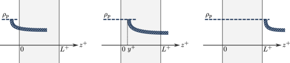
Figure 1: Diagrammatic representation of the three terms appearing in Eq. (2) where the gluon is emitted before, inside or after the medium.

The propagation of the gluon inside the medium is described by the scalar retarded propagator

$$\mathcal{G}^{ab}_{k^{+}}(x^{+},\mathbf{x};y^{+},\mathbf{y})=\int_{\mathbf{z}(y^{+})=\mathbf{y}}^{\mathbf{z}(x^{+})=\mathbf{x}}[\mathcal{D}\mathbf{z}(z^{+})]\text{exp}\left\{\frac{ik^{+}}{2}\int_{y^{+}}^{x^{+}}dz^{+}\dot{\mathbf{z}}^{2}(z^{+})\right\}U^{ab}(x^{+},y^{+};\mathbf{z}(z^{+})).$$ (3)

This path integral, from transverse position $\mathbf{y}$ at $y^{+}$ to $\mathbf{x}$ at $x^{+}$ along trajectory $\mathbf{z}(z^{+})$, encodes both the color rotation and the motion of the gluon in the transverse plane while traversing the medium. The propagation of the gluon outside the medium is given by the free scalar propagator

$$\mathcal{G}^{ab}_{0,k^{+}}(x^{+},\mathbf{x};y^{+},\mathbf{y})=\frac{-ik^{+}\delta^{ab}}{2\pi}\frac{\theta(x^{+}-y^{+})}{x^{+}-y^{+}}{\rm exp}\bigg{\{}\frac{ik^{+}}{2(x^{+}-y^{+})}({\mathbf{x}}-{\mathbf{y}})^{2}\bigg{\}}$$ (4)

(which can be obtained by setting $U^{ab}$ to $\delta^{ab}$ and computing the remaining integral). Finally, $U^{ab}(x^{+},y^{+};{\mathbf{x}})$ is the Wilson line which accounts for multiple gluon exchanges between the projectile and the target and it is given by the path-ordered exponential

$$U^{ab}(x^{+},y^{+};{\mathbf{x}})={\cal P}_{+}{\rm exp}\bigg{\{}ig\int_{y^{+}}^{x^{+}}dz^{+}A^{-}(z^{+},{\mathbf{x}})\bigg{\}}^{ab}\,.$$ (5)

In this approach the single inclusive gluon spectrum is given by

$$2k^{+}(2\pi)^{3}\frac{dN}{dk^{+}d^{2}\mathbf{k}}=\Big{\langle}\mathcal{M}^{a}_{\lambda}(k^{+},\mathbf{k})\mathcal{M}^{a\dagger}_{\lambda}(k^{+},\mathbf{k})\Big{\rangle}_{p,T}\ ,$$ (6)

where $\langle\cdots\rangle_{p,T}$ accounts for the average over the color configurations of the projectile and the target respectively. The explicit expression of this function is derived later in this manuscript and can be found in (27) and (4.1).

Within the same setup, single inclusive gluon production was studied in Refs. Altinoluk:2014oxa ; Altinoluk:2015gia by developing a systematic method to compute higher order corrections to the eikonal approximation (or equivalently to the shockwave approximation) that are due to the non-zero longitudinal width of the target. Specifically, the method was developed to expand the scalar retarded propagator given in Eq. (3). The expansion was performed at next-to-next-to-eikonal accuracy and the result was applied to the single inclusive gluon production process in $pA$ collisions. In the present work, we follow a different approach to account for the non-eikonal effects that stem from the finite longitudinal thickness of the target. Contrary to the studies performed in Refs. Altinoluk:2014oxa ; Altinoluk:2015gia , in the present work we discuss how to perform target averaging of non-eikonal objects that appear at the level of the squared amplitude without adopting the aforementioned eikonal expansion.

As mentioned briefly in Section 1, inclusive multigluon spectra is an essential observable for the study of particle correlations from the initial state point of view for small size systems such as $pp$ or $pA$ collisions. Within the CGC framework, these studies are usually performed in the “glasma graph approximation” Armesto:2006bv ; Dumitru:2008wn ; Dumitru:2010iy ; Ozonder:2014sra ; Ozonder:2017wmh which amounts to allowing the emission of a gluon from a single color source in the projectile and neglecting the contributions where more than one gluon is emitted from the same color source in the projectile. One important aspect of the glasma graph calculations is that it is only valid for dilute-dilute scattering processes, i.e., $pp$ collisions, because it only considers two gluon exchanges with the target. However, its extension that accounts for the multiple interactions with the target which corresponds to dilute-dense scatterings, or equivalently $pA$ collisions, was performed in Altinoluk:2018hcu ; Altinoluk:2018ogz . In a recent study Agostini:2021xca , the extension of the glasma graph calculations to compute $n$-gluon production in $pA$ collisions was developed and the four-gluon production spectrum was explicitly computed in the strict eikonal limit.

Here, we extend the eikonal calculation of the $n$-gluon spectrum to the non-eikonal case where the effects of the finite longitudinal width of the target are accounted for. The non-eikonal generalization of the eikonal $n$-gluon spectrum computed in Agostini:2021xca can be written as

$$2^{n}(2\pi)^{3n}\frac{d^{n}N}{\prod_{i=1}^{n}dk_{i}^{+}/k_{i}^{+}d^{2}\textbf{k}_{i}}= \,g^{2n}\int_{\textbf{q}_{1},\dots,\textbf{q}_{2n}}\Big{\langle}\rho_{p}^{b_{1}}(\textbf{q}_{1})\rho_{p}^{*b_{2}}(\textbf{q}_{2})\cdots\rho_{p}^{*b_{2n}}(\textbf{q}_{2n})\Big{\rangle}_{p}$$

$$\hskip-142.26378pt\times\Big{\langle}\overline{\mathcal{M}}^{a_{1}b_{1}}_{\lambda_{1}}(\underline{k}_{1},\textbf{q}_{1})\overline{\mathcal{M}}^{\dagger b_{2}a_{1}}_{\lambda_{1}}(\underline{k}_{1},\textbf{q}_{2})\cdots\overline{\mathcal{M}}^{a_{n}b_{2n-1}}_{\lambda_{n}}(\underline{k}_{n},\textbf{q}_{2n-1})\overline{\mathcal{M}}^{\dagger b_{2n}a_{n}}_{\lambda_{n}}(\underline{k}_{n},\textbf{q}_{2n})\Big{\rangle}_{T},$$ (7)

where a shorthand notation $\underline{k}\equiv(k^{+},\mathbf{k})$ is introduced. Due to the finite longitudinal extend of the target, the reduced matrix amplitude is a more complicated object compared to its eikonal limit. It includes not only the standard Wilson lines as in the case of strict eikonal limit but also the retarded scalar propagator $\mathcal{G}_{k^{+}}(x^{+},\mathbf{x};y^{+},\mathbf{y})$ (see Eq. (2)). Therefore, at the squared amplitude level one gets not only eikonal multipoles (dipoles, quadrupoles, etc.) but their non-eikonal generalizations which include scalar propagators. In the next section, we discuss how to evaluate the target averaging of such new objects that appear beyond eikonal accuracy.

3 Non-eikonal target averaging

In order to obtain an analytical result for the inclusive $n$-gluon spectra given in Eq. (2), the target average of the $2n$ reduced matrix amplitudes has to be computed. It is well known that in the strict eikonal limit of the single inclusive gluon spectrum, one ends up with the eikonal dipole function which is usually evaluated by using some model like McLerran-Venugopalan (MV) McLerran:1993ni ; McLerran:1994vd or Golec-Biernat–Wüsthoff (GBW) GolecBiernat:1998js ; GolecBiernat:1999qd . However, for two or more gluons multipole functions such as quadrupoles, sextuples, etc., appear. In order to easily compute the target averaging of these multipole functions, the Area Enhancement (AE) model is introduced in Refs. Kovner:2017ssr ; Kovner:2018vec ; Altinoluk:2018ogz . This model is based on the following ansatz: Any multipole can be written in terms of dipole functions through a Wick expansion for those configurations of multipole functions that maximize the phase space integration, up to terms that are suppressed by the collision area. In other words, in the AE model, after the integration over the phase space, the Wilson lines can approximately be described by a Gaussian distribution up to the corrections that are of the order of the inverse of the phase space area. In this section, we will generalize the target averaging of eikonal two point functions (eikonal dipole functions) to compute the non-eikonal two point functions (i.e., non-eikonal dipole functions) that appear in the single inclusive gluon production when one includes the target finite longitudinal width effects. Then, these results will be used together with the AE argument to study the non-eikonal multigluon spectra.

Non-eikonal single inclusive gluon spectrum is given by setting $n=1$ in Eq. (2), which requires the evaluation of the following three objects:

$$\frac{1}{N_{c}^{2}-1}\Big{\langle}\text{Tr}\left[U_{\mathbf{y}}(x^{+},y^{+})U^{\dagger}_{\bar{\mathbf{y}}}(x^{+},y^{+})\right]\Big{\rangle}_{T} \equiv d^{(0)}(x^{+},y^{+}|{\mathbf{y}},\bar{\mathbf{y}}),$$ (8)

$$\frac{1}{N_{c}^{2}-1}\Big{\langle}\text{Tr}\left[\mathcal{G}_{k^{+}}(x^{+},\textbf{x};y^{+},\textbf{y})U_{\bar{\textbf{y}}}^{\dagger}(x^{+},y^{+})\right]\Big{\rangle}_{T} \equiv d^{(1)}(x^{+},y^{+}|{\mathbf{x}},{\mathbf{y}},k^{+};\bar{\mathbf{y}}),$$ (9)

$$\frac{1}{N_{c}^{2}-1}\Big{\langle}\text{Tr}\left[{\cal G}_{k_{1}^{+}}(x^{+},{\mathbf{x}};y^{+},{\mathbf{y}}){\cal G}_{k_{2}^{+}}^{\dagger}(x^{+},\bar{\mathbf{x}};y^{+},\bar{\mathbf{y}})\right]\Big{\rangle}_{T} \equiv d^{(2)}(x^{+},y^{+}|{\mathbf{x}},{\mathbf{y}},k_{1}^{+};\bar{\mathbf{x}},\bar{\mathbf{y}},k_{2}^{+}),$$ (10)

where we have written $U_{\mathbf{x}}(x^{+},y^{+})\equiv U(x^{+},y^{+};\mathbf{x})$ for simplicity. It is straightforward to note that $d^{(0)}(x^{+},y^{+}|{\mathbf{y}},\bar{\mathbf{y}})$ given in Eq. (8) can be identified with the eikonal dipole function evaluated over a finite longitudinal extent $z^{+}\in[y^{+},x^{+}]$ of the target. The functions defined in Eqs. (9) and (10) are non-eikonal generalizations of the dipole function.

For simplicity, we assume that the eikonal dipole function is described by the GBW model which is valid as long as the dipole size is much smaller than $\Lambda_{\rm QCD}^{-1}$. In this case, the eikonal dipole function reads

$$d^{(0)}(x^{+},y^{+}|{\mathbf{y}},\bar{\mathbf{y}})=\text{exp}\left\{-\frac{q_{s}^{2}(x^{+},y^{+})}{4}(\mathbf{x}-\mathbf{y})^{2}\right\},$$ (11)

where $q_{s}(x^{+},y^{+})$ can be identified as the effective saturation momentum in a longitudinal slice $[y^{+},x^{+}]$ of the target. Within the MV model, saturation momentum can be defined as

$$Q_{s}^{2}=\frac{g^{4}\,C_{R}\,\mu^{2}}{4\pi}\ ,$$ (12)

with $\mu^{2}$ the color density of the target and $C_{R}$ the Casimir of the projectile parton interacting with the target. With this definition of the saturation momentum, the effective saturation momentum $q_{s}(x^{+},y^{+})$ can be defined as

$$q_{s}^{2}(x^{+},y^{+})=\frac{g^{4}C_{R}}{4\pi}\int_{y^{+}}^{x^{+}}dz^{+}\tilde{\mu}^{2}(z^{+}).$$ (13)

Thus, assuming that the color density $\tilde{\mu}^{2}(z^{+})$ is constant along the target longitudinal extent, i.e., $\tilde{\mu}^{2}(z^{+})=\mu^{2}/L^{+}$, the effective saturation momentum takes the following form:

$$q_{s}^{2}(x^{+},y^{+})=\frac{x^{+}-y^{+}}{L^{+}}Q_{s}^{2}.$$ (14)

The object defined in Eq. (9) is one of the generalizations of the eikonal dipole function which stems from the finite longitudinal extent of the target and we refer to it as the $1^{\rm st}$ order NE dipole function. It requires averaging over the scalar propagator $\mathcal{G}_{k^{+}}(x^{+},\mathbf{x};y^{+},\mathbf{y})$ defined in Eq. (3) and therefore implies solving a path integral. In order to do so, we discretize the longitudinal space into $N$ slices where each discretized point is labeled as $z_{i}^{+}$. In this case, the scalar propagator can be written as Altinoluk:2014oxa ; Altinoluk:2015gia ; Mehtar-Tani:2006vpj

$$\mathcal{G}^{ab}_{k^{+}}(\underline{x},\underline{y})=\lim_{N\rightarrow\infty}\Theta(x^{+}-y^{+})\int\left(\prod_{n=1}^{N-1}d^{2}\textbf{z}_{n}\right)\left(\frac{-ik^{+}N}{2(x^{+}-y^{+})}\right)^{N}$$

$$\hskip 113.81102pt\times\text{exp}\left\{\frac{ik^{+}N}{2(x^{+}-y^{+})}\sum_{n=1}^{N}(\textbf{z}_{n}-\textbf{z}_{n-1})^{2}\right\}\prod_{n=1}^{N}U^{ab}_{\mathbf{z}_{n}}(z_{n-1}^{+},z_{n}^{+}),$$ (15)

where we have defined ${\underline{x}}\equiv(x^{+},\mathbf{x})$. This equation describes the discrete random walk of the emitted gluon through the transverse points $\mathbf{z}_{n}(z_{n}^{+})$ inside the target. The emitted gluon is propagated from $\mathbf{z}_{0}(z_{0}^{+})=\mathbf{y}$ with $z_{0}^{+}=y^{+}$ to $\mathbf{z}_{N}(z_{N}^{+})=\mathbf{x}$ with $z_{N}^{+}=x^{+}$. The only dependence on the target configuration in Eq. (3) appears through the discretized Wilson lines, $U^{ab}_{\mathbf{z}_{n}}(z_{n-1}^{+},z_{n}^{+})$, that account for the eikonal propagation of the gluon in each longitudinal slice. Thus, the $1^{\rm st}$ order NE dipole function defined in Eq. (9) can be written as

$$d^{(1)}(x^{+},y^{+}|{\mathbf{x}},{\mathbf{y}},k^{+};\bar{\mathbf{y}})=\lim_{N\rightarrow\infty}\int\left(\prod_{n=1}^{N-1}d^{2}\textbf{z}_{n}\right)\text{exp}\left\{\frac{ik^{+}N}{2(x^{+}-y^{+})}\sum_{n=1}^{N}(\textbf{z}_{n}-\textbf{z}_{n-1})^{2}\right\}$$

$$\hskip 85.35826pt\times\left(\frac{-ik^{+}N}{2(x^{+}-y^{+})}\right)^{N}\Bigg{\langle}\text{Tr}\left[\left(\prod_{n=1}^{N}U_{\mathbf{z}_{n}}(z_{n-1}^{+},z_{n}^{+})\right)U^{\dagger}_{\mathbf{\bar{y}}}(x^{+},y^{+})\right]\Bigg{\rangle}_{T}.$$ (16)

This expression can be further simplified by realizing that, due to the properties of path-ordered exponentials, the Wilson line evaluated over some longitudinal extent $[y^{+},x^{+}]$ can be factorized into a product of independent contributions at each slice of the discretized axis:

$$U_{\mathbf{x}}(x^{+},y^{+})=\prod_{i=1}^{n}U_{\mathbf{x}}(x_{i-1}^{+},x_{i}^{+}),$$ (17)

where $x_{0}^{+}=y^{+}$ and $x_{n}^{+}=x^{+}$. Moreover, noting that the MV model is local in the longitudinal direction which implies that the average of Wilson lines evaluated at different points on the longitudinal axis factorizes into independent averages, we simplify the target average in Eq. (3) to

$$\Bigg{\langle}\text{Tr}\left[\left(\prod_{n=1}^{N}U_{\mathbf{z}_{n}}(z_{n-1}^{+},z_{n}^{+})\right)U^{\dagger}_{\mathbf{\bar{y}}}(x^{+},y^{+})\right]\Bigg{\rangle}_{T}$$

$$= \prod_{n=1}^{N}\Bigg{\langle}\text{Tr}\left[U_{\mathbf{z}_{n}}(z_{n-1}^{+},z_{n}^{+})U^{\dagger}_{\mathbf{\bar{y}}}(z_{n-1}^{+},z_{n}^{+})\right]\Bigg{\rangle}_{T}.$$ (18)

Finally, by using the local GBW model given in Eq. (11) and noting that $z_{i}^{+}-z_{i-1}^{+}=L^{+}/N$, the $1^{\rm st}$ order NE dipole function takes the following form:

$$d^{(1)}(x^{+},y^{+}|{\mathbf{x}},{\mathbf{y}},k^{+};\bar{\mathbf{y}})=\lim_{N\rightarrow\infty}\int\left(\prod_{n=1}^{N-1}d^{2}\textbf{z}_{n}\right)\left(\frac{-ik^{+}N}{2(x^{+}-y^{+})}\right)^{N}$$

$$\hskip 85.35826pt\times\text{exp}\left\{\frac{ik^{+}N}{2(x^{+}-y^{+})}\sum_{n=1}^{N}(\textbf{z}_{n}-\textbf{z}_{n-1})^{2}-\frac{Q_{s}^{2}}{4N}\sum_{n=1}^{N}(\mathbf{z}_{n}-\mathbf{\bar{y}})^{2}\right\}.$$ (19)

In the continuum limit, by defining $\mathbf{r}=\mathbf{z}-\mathbf{\bar{y}}$, Eq. (3) can be written as

$$d^{(1)}(x^{+},y^{+}|{\mathbf{x}},{\mathbf{y}},k^{+};\bar{\mathbf{y}})=\int[\mathcal{D}\mathbf{r}]\text{exp}\left\{\int_{y^{+}}^{x^{+}}dz^{+}\left[\frac{ik^{+}}{2}\dot{\mathbf{r}}^{2}-\frac{Q_{s}^{2}}{4L^{+}}\mathbf{r}^{2}\right]\right\}.$$ (20)

Two comments are in order here. First, the result given in Eq. (20) can be obtained in a straightforward manner by using the expression for the scalar propagator $\mathcal{G}_{k^{+}}(x^{+},\mathbf{x};y^{+},\mathbf{y})$ given in Eq. (3) in the definition of the $1^{\rm st}$ order NE dipole function and adopting the GBW model directly without introducing the discretization along the longitudinal axis. However, the way that Eq. (20) is obtained above justifies the use of the locality argument which plays a crucial role in our discussion. Second, Eq. (20) is the well known path integral of the harmonic oscillator with “mass” $k^{+}/2$ and imaginary “frequency” $\sqrt{-iQ_{s}^{2}/2L^{+}k^{+}}$ that is frequently used in jet quenching calculations (see for example Mehtar-Tani:2013pia ). For completeness, we compute this integral in Appendix A with the result given in (A). Thus, after performing the path integral, the $1^{\rm st}$ order NE dipole function reads

$$d^{(1)}(x^{+},y^{+}|{\mathbf{x}},{\mathbf{y}},k_{i}^{+};\bar{\mathbf{y}})=\frac{-Q_{s}^{2}}{4\pi\epsilon_{i}\sin\frac{\epsilon_{i}\Delta^{+}}{L^{+}}}\text{exp}\left\{\frac{Q_{s}^{2}}{4\epsilon_{i}}\left[\frac{\mathbf{a}_{0}^{2}+\mathbf{a}_{N}^{2}}{\tan\frac{\epsilon_{i}\Delta^{+}}{L^{+}}}-2\frac{\mathbf{a}_{0}\cdot\mathbf{a}_{N}}{\sin\frac{\epsilon_{i}\Delta^{+}}{L^{+}}}\right]\right\},$$ (21)

where we have defined $\Delta^{+}=x^{+}-y^{+}$, $\mathbf{a}_{0}=\mathbf{y}-\mathbf{\bar{y}}$, $\mathbf{a}_{N}=\mathbf{x}-\mathbf{\bar{y}}$ and

$$\epsilon_{i}^{2}=\frac{Q_{s}^{2}L^{+}}{2ik_{i}^{+}}.$$ (22)

Note that $\epsilon_{i}^{2}$ is a dimensionless parameter that vanishes in the eikonal limit ($k_{i}^{+}\to\infty$ and $L^{+}\to 0$). Its role is to weight the strength of the finite longitudinal width effects and we will refer to it as the non-eikonal parameter.

The next two-point function that we consider is defined in Eq. (10). It is referred to as the $2^{\rm nd}$ order NE dipole function which can be computed in the same manner as the $1^{\rm st}$ order one. By using the GBW model and the locality of the MV model we can write it as

$$d^{(2)}(x^{+},y^{+}|{\mathbf{x}},{\mathbf{y}},k_{1}^{+};\bar{\mathbf{x}},\bar{\mathbf{y}},k_{2}^{+})$$

$$\hskip 85.35826pt=\int[\mathcal{D}\mathbf{r}][\mathcal{D}\mathbf{\bar{r}}]\text{exp}\left\{\int_{y^{+}}^{x^{+}}dz^{+}\left[\frac{ik_{1}^{+}}{2}\mathbf{\dot{r}}^{2}-\frac{ik_{2}^{+}}{2}\mathbf{\dot{\bar{r}}}^{2}-\frac{Q_{s}^{2}}{4L^{+}}(\mathbf{r}-\mathbf{\bar{r}})^{2}\right]\right\},$$ (23)

where $\mathbf{r}(y^{+})=\mathbf{y}$, $\mathbf{r}(x^{+})=\mathbf{x}$, $\mathbf{\bar{r}}(y^{+})=\mathbf{\bar{y}}$ and $\mathbf{\bar{r}}(x^{+})=\mathbf{\bar{x}}$. This equation can be identified with the path integral of two coupled harmonic oscillators which can be decoupled. The solution is also derived in Appendix A and the final result is given in Eq. (A). Thus, the $2^{\rm nd}$ order NE dipole function reads

$$d^{(2)}(x^{+},y^{+}|{\mathbf{x}},{\mathbf{y}},k_{1}^{+};\bar{\mathbf{x}},\bar{\mathbf{y}},k_{2}^{+})=\frac{-Q_{s}^{4}}{(4\pi)^{2}}\frac{\epsilon_{-}L^{+}}{\Delta^{+}\epsilon_{1}^{2}\epsilon_{2}^{2}\sin\frac{\Delta^{+}\epsilon_{-}}{L^{+}}}{\rm exp}\Bigg{\{}\frac{Q_{s}^{2}}{4\epsilon_{-}^{2}}\Bigg{(}\frac{\epsilon_{-}(\mathbf{r}_{0}^{2}+\mathbf{r}_{N}^{2})}{\tan\frac{\Delta^{+}\epsilon_{-}}{L^{+}}}$$

$$\hskip 71.13188pt-2\frac{\epsilon_{-}\mathbf{r}_{0}\cdot\mathbf{r_{N}}}{\sin\frac{\Delta^{+}\epsilon_{-}}{L^{+}}}-\frac{L^{+}}{\Delta^{+}\epsilon_{1}^{2}\epsilon_{2}^{2}\epsilon_{+}^{4}}\left[2\epsilon_{1}^{2}\epsilon_{2}^{2}(\mathbf{r}_{N}-\mathbf{r}_{0})-\epsilon_{+}^{2}\epsilon_{-}^{2}(\mathbf{b}_{N}-\mathbf{b}_{0})\right]^{2}\Bigg{)}\Bigg{\}},$$ (24)

where we have defined for simplicity $\epsilon_{\pm}^{2}=\epsilon_{1}^{2}\pm\epsilon_{2}^{2}$, $\mathbf{r}_{0}=\mathbf{y}-\mathbf{\bar{y}}$, $\mathbf{r}_{N}=\mathbf{x}-\mathbf{\bar{x}}$, $\mathbf{b}_{0}=(k_{1}^{+}\mathbf{y}+k_{2}^{+}\mathbf{\bar{y}})/(k_{1}^{+}+k_{2}^{+})$ and $\mathbf{b}_{N}=(k_{1}^{+}\mathbf{x}+k_{2}^{+}\mathbf{\bar{x}})/(k_{1}^{+}+k_{2}^{+})$.

We would like to emphasize that this solution is novel and only in the limit $k_{2}^{+}=k_{1}^{+}$ it simplifies and leads to the known results Casalderrey-Solana:2007knd ; Zakharov:1998sv ; Blaizot:2012fh ; Apolinario:2014csa .

$$d^{(2)}(x^{+},y^{+}|{\mathbf{x}},{\mathbf{y}},k_{1}^{+};\bar{\mathbf{x}},\bar{\mathbf{y}},k_{1}^{+})=-\left(\frac{L^{+}Q_{s}^{2}}{4\pi\Delta^{+}\epsilon_{1}^{2}}\right)^{2}$$

$$\hskip 28.45274pt\times{\rm exp}\Bigg{\{}-\frac{Q_{s}^{2}}{12\epsilon_{1}^{2}}\Bigg{[}\epsilon_{1}^{2}\frac{\Delta^{+}}{L^{+}}(\mathbf{r}_{0}^{2}+\mathbf{r}_{N}^{2}+\mathbf{r}_{0}\cdot\mathbf{r}_{N})-6\frac{L^{+}}{\Delta^{+}}(\mathbf{r}_{N}-\mathbf{r}_{0})\cdot(\mathbf{b}_{N}-\mathbf{b}_{0})\Bigg{]}\Bigg{\}}$$ (25)

which is required for single inclusive gluon production or medium-induced gluon radiation. But the more general result for $k_{2}^{+}\neq k_{1}^{+}$ is required for double inclusive gluon production, that we analyse below (see also Appendix B).

With Eqs. (11), (21) and (3) we have determined the non-eikonal dipole functions evaluated within a longitudinal extent $\Delta^{+}$ of the target medium. We note that these functions are extensively used by the jet quenching community where the effects of the parton propagation within a dense medium is computed. In that case, the GBW model is usually referred to as the harmonic oscillator approximation and the effective saturation scale defined in Eq. (11) is written

$$q_{s}^{2}(x^{+},y^{+})=\int_{y^{+}}^{x^{+}}\hat{q}(z^{+})dz^{+},$$ (26)

where $\hat{q}(z^{+})$ is the medium transport coefficient. For a static homogeneous medium in which $\hat{q}(z^{+})$ is constant, we get $\hat{q}=Q_{s}^{2}/L^{+}$.

Before we conclude this section, we would like to comment on the computation of the higher order functions, i.e., multipoles, where one has to evaluate the non-eikonal target average of multiple Wilson lines and scalar propagators. As stated shortly at the beginning of this section, in order to compute the NE multipoles we use the AE model. This model is based on the chromo-electric domain structure in the target transverse plane and leads to a similar result when compared with the MV model. The advantage of this approach is that, upon integration over the transverse phase space, the Wilson lines follow approximately a Gaussian distribution – with the non-Gaussian corrections suppressed by the collision area – and therefore allows one to adopt Wick’s theorem. However, in the case of a target with a finite longitudinal extent, one should be more careful since the chromo-electric domains may decohere in the longitudinal direction.

To justify the application of the AE model in target ensembles with non-zero width, $L^{+}$, we examine the space-time kinematics of the interaction in the center-of-mass (CoM) frame. In this frame the Lorentz contracted target width is $L^{+}\sim A^{1/3}/\sqrt{s_{\rm NN}}$. On the other hand, the chromo-electric fields are defined by the low-$x$ gluons which have the following spread in the longitudinal direction: $\Delta x^{+}\sim 1/q^{-}=A/(xQ_{T}^{-})$, where $Q_{T}^{-}=A\sqrt{s_{\rm NN}}/\sqrt{2}$ and $q^{-}$ are the longitudinal momentum (in the CoM frame) of the target and the gluon respectively. Thus, as long as $\Delta x^{+}\gg L^{+}$ the domain structure of the target will not decohere within its extent and the AE model is justified. Therefore, for $L^{+}/\Delta x^{+}\sim xA^{1/3}\ll 1$ the Area Enhancement model should be a good approximation in the non-eikonal case.

4 Non-Eikonal single inclusive gluon production

Before computing the non-eikonal multi gluon production, we first consider the single inclusive case as a warm up. In this section, we first derive the analytical solutions of the non-eikonal single inclusive spectrum, then perform the numerical analysis of these results and finally compare our results with the ones that exist in the literature (specifically with the results of Ref. Altinoluk:2014oxa ; Altinoluk:2015gia ).

4.1 Analytical results

The non-eikonal single inclusive gluon spectrum is given by Eq. (2) for $n=1$, which reads

$$(2\pi)^{3}(2k^{+})\frac{dN}{dk^{+}d^{2}\textbf{k}}=g^{2}\int_{\textbf{q}_{1},\textbf{q}_{2}}\big{\langle}\rho^{b_{1}}(\textbf{q}_{1})\rho^{*b_{2}}(\textbf{q}_{2})\big{\rangle}_{p}\big{\langle}\overline{\mathcal{M}}^{b_{1}a_{1}}_{\lambda}(\underline{k},\textbf{q}_{1})\overline{\mathcal{M}}^{\dagger a_{1}b_{2}}_{\lambda}(\underline{k},\textbf{q}_{2})\big{\rangle}_{T}.$$ (27)

We employ the MV model to compute the averaging over the projectile color sources:

$$\big{\langle}\rho^{b_{1}}(\textbf{q}_{1})\rho^{*b_{2}}(\textbf{q}_{2})\big{\rangle}_{p}=\frac{\delta^{b_{1}b_{2}}}{N_{c}^{2}-1}\mu^{2}(\mathbf{q}_{1},-\mathbf{q}_{2}),$$ (28)

where the factor $1/(N_{c}^{2}-1)$ is introduced by convenience but will not be relevant in the analysis performed in this manuscript. Since this contribution is proportional to $\delta^{b_{1}b_{2}}$, it leads to a color trace of the reduced amplitudes in Eq. (27). By using the expression for the reduced amplitude given in Eq. (2), the target average of the reduced amplitudes for single inclusive gluon spectrum can be written as

$$\frac{1}{N_{c}^{2}-1}\Big{\langle}\text{Tr}\left[\overline{\mathcal{M}}_{\lambda}(\underline{k},\textbf{q}_{1})\overline{\mathcal{M}}^{\dagger}_{\lambda}(\underline{k},\textbf{q}_{2})\right]\Big{\rangle}_{T}=\int_{\textbf{y},\bar{\textbf{y}}}e^{i{\mathbf{q}}_{1}\cdot{\mathbf{y}}-i{\mathbf{q}}_{2}\cdot\bar{\mathbf{y}}}\bigg{\{}\frac{2}{{\mathbf{k}}^{2}}e^{-i{\mathbf{k}}\cdot({\mathbf{y}}-\bar{\mathbf{y}})}d^{(0)}(L^{+},0|{\mathbf{y}};\bar{\mathbf{y}})$$

$$\hskip 170.71652pt+2\frac{{\mathbf{q}}_{1}\cdot{\mathbf{q}}_{2}}{{\mathbf{q}}_{1}^{2}{\mathbf{q}}_{2}^{2}}\int_{{\mathbf{x}},\bar{\mathbf{x}}}e^{-i{\mathbf{k}}\cdot({\mathbf{x}}-\bar{\mathbf{x}})}d^{(2)}(L^{+},0|,{\mathbf{x}},{\mathbf{y}},k^{+};\bar{\mathbf{x}},\bar{\mathbf{y}},k^{+})$$

$$-4\frac{{\mathbf{k}}\cdot{\mathbf{q}}_{1}}{{\mathbf{k}}^{2}{\mathbf{q}}_{1}^{2}}\int_{\mathbf{x}}e^{-i{\mathbf{k}}\cdot({\mathbf{x}}-\bar{\mathbf{y}})}d^{(1)}(L^{+},0|{\mathbf{x}},{\mathbf{y}},k^{+};\bar{\mathbf{y}})$$

$$+2\frac{{\mathbf{k}}^{i}}{{\mathbf{k}}^{2}}\frac{1}{k^{+}}\int_{0}^{L^{+}}dy^{+}\int_{{\mathbf{x}}}e^{-i{\mathbf{k}}\cdot({\mathbf{x}}-\bar{\mathbf{y}})}d^{(0)}(y^{+},0|{\mathbf{y}};\bar{\mathbf{y}})\big{[}\partial_{{\mathbf{y}}^{i}}d^{(1)}(L^{+},0|{\mathbf{x}},{\mathbf{y}},k^{+};\bar{\mathbf{y}})\big{]}$$

$$-2\frac{{\mathbf{q}}_{1}^{i}}{{\mathbf{q}}_{1}^{2}}\frac{1}{k^{+}}\int_{0}^{L^{+}}dy^{+}\int_{{\mathbf{x}},\bar{\mathbf{x}},{\mathbf{u}}}e^{-i{\mathbf{k}}\cdot({\mathbf{x}}-\bar{\mathbf{x}})}\big{[}\partial_{\bar{\mathbf{y}}^{i}}d^{(2)}(L^{+},0|,{\mathbf{x}},{\mathbf{y}},k^{+};\bar{\mathbf{x}},\bar{\mathbf{y}},k^{+})\big{]}$$

$$\hskip 256.0748pt\times d^{(1)}(L^{+},0|{\mathbf{x}},{\mathbf{y}},k^{+};\bar{\mathbf{y}})$$

$$+\frac{1}{(k^{+})^{2}}\int_{0}^{L^{+}}dy^{+}\int_{y^{+}}^{L^{+}}d\bar{y}^{+}\int_{{\mathbf{x}},\bar{\mathbf{x}},{\mathbf{u}}}e^{-{\mathbf{k}}\cdot({\mathbf{x}}-\bar{\mathbf{x}})}\big{[}\partial_{\bar{\mathbf{y}}^{i}}d^{(2)}(L^{+},0|,{\mathbf{x}},{\mathbf{y}},k^{+};\bar{\mathbf{x}},\bar{\mathbf{y}},k^{+})\big{]}$$

$$\hskip 142.26378pt\times\big{[}\partial_{{\mathbf{y}}^{i}}d^{(1)}(L^{+},0|{\mathbf{x}},{\mathbf{y}},k^{+};\bar{\mathbf{y}})\big{]}d^{(0)}(y^{+},0|{\mathbf{y}};\bar{\mathbf{y}})\bigg{\}}+\mathbf{c.c.},$$ (29)

where we have used the convolution property of the scalar propagator

$${\cal G}_{k^{+}}(x^{+},\mathbf{x};y^{+},\mathbf{y})=\int_{\mathbf{u}}{\cal G}_{k^{+}}(x^{+},\mathbf{x};z^{+},\mathbf{u}){\cal G}_{k^{+}}(z^{+},\mathbf{u};y^{+},\mathbf{y}),\ \ y^{+}<z^{+}<x^{+},$$ (30)

in order to break the target average of the scalar propagator into its local pieces where the number of objects is fixed.

It is worth mentioning that since we are using the GBW model (i.e., a Gaussian form) for the non-eikonal dipole functions, all the integrals over the transverse coordinates or transverse momenta appearing in Eq. (4.1), or in general in this manuscript, are of the form

$$\int_{\mathbf{x}}(a+\mathbf{b}^{i}\mathbf{x}^{i}+\mathbf{c}^{i}\mathbf{d}^{j}\mathbf{x}^{i}\mathbf{x}^{j})e^{-A\mathbf{x}^{2}+\mathbf{B}\cdot\mathbf{x}}=\frac{\pi}{A}e^{\frac{\mathbf{B}^{2}}{4A}}\Bigg{[}a+\mathbf{b}^{i}\frac{\mathbf{B}^{i}}{2A}+\frac{\mathbf{c}^{i}\mathbf{d}^{j}}{2A}\left(\delta^{ij}+\frac{\mathbf{B}^{i}\mathbf{B}^{j}}{2A}\right)\Bigg{]},$$ (31)

and, therefore, although very tedious in some cases, it is straightforward to compute them. Moreover, the argument of the integrals over $\mathbf{y}$ and $\mathbf{\bar{y}}$ is translational invariant under these coordinates and thus the integral is proportional to $\delta^{(2)}(\mathbf{q}_{1}-\mathbf{q}_{2})$. Then, the single inclusive gluon spectrum given in Eq. (27) can explicitly be written as

$$\frac{dN}{d\eta d^{2}\textbf{k}}=\frac{g^{2}\pi B_{p}}{(2\pi)^{3}}\int_{\textbf{q}}\operatorname{Re}\Big{\{}\mathcal{I}_{\text{aft-aft}}+\mathcal{I}_{\text{bef-bef}}+\mathcal{I}_{\text{aft-bef}}+\mathcal{I}_{\text{aft-in}}+\mathcal{I}_{\text{in-bef}}+\mathcal{I}_{\text{in-in}}\Big{\}},$$ (32)

where we have used the fact that $\mu^{2}(\mathbf{q},-\mathbf{q})=\pi B_{p}$, with $B_{p}$ the gluonic transverse area of the projectile. We have also changed our notation from the longitudinal momentum to rapidty: $dk^{+}/k^{+}=d\eta$. The terms that appear in the argument of the integral in Eq. (32) result from squaring the contributions in Eq. (2) where the gluon is emitted before, after or inside the target medium (see Fig. 2).

Figure 2: All possible contributions to the single gluon spectrum given in Eq. (32), which result from squaring the amplitude of a gluon being emitted before, during (inside) or after the interaction of the source with the target.

By using the expressions for the eikonal dipole function and the two non-eikonal dipole functions, explicit expressions of each contribution in Eq. (32) can be computed. Let us start with the $\mathcal{I}_{\text{aft-aft}}$ term. This term is the contribution where the gluon is emitted after the interaction of the source with the target on both sides of the cut. It reads

$$\mathcal{I}_{\text{aft-aft}}=\frac{2}{{\mathbf{k}}^{2}}\int_{\mathbf{r}}e^{-i(\mathbf{k}-\mathbf{q})\cdot\mathbf{r}}d^{(0)}\left(L^{+},0\Big{|}\frac{{\mathbf{r}}}{2};-\frac{{\mathbf{r}}}{2}\right)=\frac{8\pi}{Q_{s}^{2}}\frac{1}{\textbf{k}^{2}}\text{exp}\left\{-\frac{(\textbf{k}-\textbf{q})^{2}}{Q_{s}^{2}}\right\}.$$ (33)

Note that we have dropped the dependence on the impact parameter $\mathbf{b}$ because the eikonal dipole function is translational invariant.

The next contribution in Eq. (32) is the $\mathcal{I}_{\text{bef-bef}}$ term which corresponds to the emission of the gluon before the interaction of the source with the target on both sides of the cut. It reads

$$\mathcal{I}_{\text{bef-bef}}=\frac{2}{\mathbf{q}^{2}}\int_{{\mathbf{r}}}e^{-i\mathbf{q}\cdot\mathbf{r}}\int_{{\mathbf{x}},\bar{\mathbf{x}}}e^{-i{\mathbf{k}}\cdot({\mathbf{x}}-\bar{\mathbf{x}})}d^{(2)}\left(L^{+},0\Big{|},{\mathbf{x}},\mathbf{b}+\frac{{\mathbf{r}}}{2},k^{+};\bar{\mathbf{x}},\mathbf{b}-\frac{{\mathbf{r}}}{2},k^{+}\right).$$ (34)

We would like to mention that we keep the impact parameter $\mathbf{b}$ dependence in Eq. (34) for consistency of the notation but, after performing the Fourier transforms, the final result is translationally invariant, i.e., independent of $\mathbf{b}$ (see also the comment before Eq. (32)). Moreover, the Fourier transform of the $2^{\rm nd}$ order NE dipole when the two longitudinal momenta are equal (as in the case of Eq. (3)) reads

$$\hskip-14.22636pt\int_{\textbf{x},\bar{\textbf{x}}}e^{-i\textbf{k}(\textbf{x}-\bar{\textbf{x}})}d^{(2)}(x^{+},y^{+}|{\mathbf{x}},{\mathbf{y}},k^{+};\bar{\mathbf{x}},\bar{\mathbf{y}},k^{+})=\text{exp}\left\{-\frac{\Delta^{+}Q_{s}^{2}}{4L^{+}}(\mathbf{y}-\mathbf{\bar{y}})^{2}-i\mathbf{k}\cdot(\mathbf{y}-\mathbf{\bar{y}})\right\},$$ (35)

which shows that in this case the $2^{\rm nd}$ order NE dipole function does not provide any non-eikonal correction. As we shall see later, this is not the case when the two longitudinal momenta are different. Thus, the result for the $\mathcal{I}_{\text{bef-bef}}$ contribution reads

$$\mathcal{I}_{\text{bef-bef}}=\frac{8\pi}{Q_{s}^{2}}\frac{1}{\textbf{q}^{2}}\text{exp}\left\{-\frac{(\textbf{k}-\textbf{q})^{2}}{Q_{s}^{2}}\right\}.$$ (36)

The $\mathcal{I}_{\text{aft-bef}}$ term corresponds to the case where the gluon is emitted before the interaction of the source with target on one side of the cut and after on the other side. This term can be written as

$$\mathcal{I}_{\text{aft-bef}}=-4\frac{{\mathbf{k}}\cdot{\mathbf{q}}}{{\mathbf{k}}^{2}{\mathbf{q}}^{2}}\int_{{\mathbf{r}}}e^{-i\mathbf{q}\cdot\mathbf{r}}\int_{\mathbf{x}}e^{-i{\mathbf{k}}\cdot({\mathbf{x}}-\mathbf{b}+\mathbf{r}/2)}d^{(1)}\left(L^{+},0\Big{|}{\mathbf{x}},\mathbf{b}+\frac{{\mathbf{r}}}{2},k^{+};\mathbf{b}-\frac{{\mathbf{r}}}{2}\right).$$ (37)

Noting that the Fourier transform of the $1^{\rm st}$ order NE dipole given in Eq. (21) reads

$$\int_{\textbf{x}}e^{-i\textbf{k}\textbf{x}}d_{k^{+}}^{(1)}(x^{+},y^{+}|{\mathbf{x}},{\mathbf{y}};\bar{\mathbf{y}})$$

$$\hskip 28.45274pt=\frac{1}{\sin\frac{\Delta^{+}\epsilon}{L^{+}}}e^{-i\mathbf{k}\cdot\mathbf{\bar{y}}}\text{exp}\left\{\left(-\frac{Q_{s}^{2}}{4\epsilon}(\mathbf{y}-\mathbf{\bar{y}})^{2}+\epsilon\frac{\mathbf{k}^{2}}{Q_{s}^{2}}\right)\tan\frac{\Delta^{+}\epsilon}{L^{+}}+i\frac{\mathbf{k}\cdot(\mathbf{y}-\mathbf{\bar{y}})}{\sin\frac{\Delta^{+}\epsilon}{L^{+}}}\right\},$$ (38)

$\mathcal{I}_{\text{aft-bef}}$ takes the following form:

$$\mathcal{I}_{\text{aft-bef}}=-\frac{16\pi\epsilon}{Q_{s}^{2}\sin\epsilon}\frac{\textbf{k}\cdot\textbf{q}}{\textbf{k}^{2}\textbf{q}^{2}}\text{exp}\left\{-\frac{\epsilon}{Q_{s}^{2}}\left[\frac{\textbf{k}^{2}+\textbf{q}^{2}}{\tan\epsilon}-2\frac{\textbf{k}\cdot\textbf{q}}{\sin\epsilon}\right]\right\}.$$ (39)

It is straightforward to realize that from this equation one can recover the results coming from the GBW model by considering the eikonal limit $|\epsilon^{2}|\to 0$ (see the dependence on k and q in Eq. (33)).

$\mathcal{I}_{\text{aft-in}}$ corresponds to the case where the gluon is emitted after the interaction of the source with the target on one side of the cut and inside the target on the other side. This contribution can be written

$$\mathcal{I}_{\text{aft-in}}=\frac{{\mathbf{k}}^{i}}{{\mathbf{k}}^{2}}\frac{2}{k^{+}}\int_{0}^{L^{+}}dy^{+}\int_{{\mathbf{x}},\mathbf{r}}e^{-i\mathbf{q}\cdot\mathbf{r}-i{\mathbf{k}}\cdot({\mathbf{x}}-\bar{\mathbf{y}})}d^{(0)}(y^{+},0|{\mathbf{y}};\bar{\mathbf{y}})\big{[}\partial_{{\mathbf{y}}^{i}}d^{(1)}(L^{+},y^{+}|{\mathbf{x}},{\mathbf{y}},k^{+};\bar{\mathbf{y}})\big{]},$$ (40)

where $\mathbf{y}=\mathbf{b}+\frac{\mathbf{r}}{2}$, $\mathbf{\bar{y}}=\mathbf{b}-\frac{\mathbf{r}}{2}$ and $y^{+}$ is the longitudinal coordinate where the gluon is emitted inside the target. Using Eq. (4.1) and defining $\alpha=\frac{L^{+}-y^{+}}{L^{+}}$ as the fraction of the target that the gluon traverses, we can write this contribution as

$$\mathcal{I}_{\text{aft-in}}=\frac{16\pi\epsilon^{3}}{Q_{s}^{4}}\int_{0}^{1}d\alpha\frac{\sec^{2}(\alpha\epsilon)}{(\epsilon\tilde{\alpha}+\tan(\alpha\epsilon))^{2}}\frac{\textbf{k}^{2}\tilde{\alpha}\epsilon+\textbf{k}\cdot\textbf{q}\sin(\alpha\epsilon)}{\textbf{k}^{2}}$$

$$\hskip 28.45274pt\times\text{exp}\left\{-\frac{\epsilon}{Q_{s}^{2}(\epsilon\tilde{\alpha}+\tan(\alpha\epsilon))}\Big{[}\textbf{k}^{2}\big{(}1-\tilde{\alpha}\epsilon\tan(\alpha\epsilon)\big{)}+\textbf{q}^{2}-2\textbf{k}\cdot\textbf{q}\sec(\alpha\epsilon)\Big{]}\right\}.$$ (41)

Here, we also introduced the notation $\tilde{\alpha}=1-\alpha$ that corresponds to the longitudinal extent of the target traversed by the source before emitting the gluon. It is worth mentioning that when the trigonometric functions are expanded to the leading order in $\epsilon$, $\mathcal{I}_{\text{aft-in}}$ is $\mathcal{O}(\epsilon^{2})$ while the first three contributions ($\mathcal{I}_{\text{aft-aft}}$, $\mathcal{I}_{\text{bef-bef}}$, $\mathcal{I}_{\text{aft-bef}}$) are $\mathcal{O}(\epsilon^{0})$. This implies that $\mathcal{I}_{\text{aft-in}}$ term is the first genuine non-eikonal contribution which is absent in the shockwave approximation.

$\mathcal{I}_{\text{in-bef}}$ term is another interference contribution that corresponds to emission of the gluon inside the target on one side of the cut and before on the other side and it can be written

$$\mathcal{I}_{\text{in-bef}}=-\frac{{\mathbf{q}}^{i}}{{\mathbf{q}}^{2}}\frac{2}{k^{+}}\int_{0}^{L^{+}}dy^{+}\int_{{\mathbf{x}},\bar{\mathbf{x}},{\mathbf{u}},\mathbf{r}}e^{-i\mathbf{q}\cdot\mathbf{r}-i{\mathbf{k}}\cdot({\mathbf{x}}-\bar{\mathbf{x}})}\big{[}\partial_{\bar{\mathbf{y}}^{i}}d^{(2)}(L^{+},y^{+}|{\mathbf{x}},{\mathbf{u}},k^{+};\bar{\mathbf{x}},\bar{\mathbf{y}},k^{+})\big{]}$$

$$\hskip 256.0748pt\times d^{(1)}(y^{+},0|{\mathbf{u}},{\mathbf{y}},k^{+};\bar{\mathbf{y}}).$$ (42)

This integral can be performed in the same manner as before, using Eq. (35) and the same definition of $\alpha$. The result reads

$$\mathcal{I}_{\text{in-bef}}=-\frac{16\pi\epsilon^{3}}{Q_{s}^{4}}\int_{0}^{1}d\alpha\frac{\sec^{2}(\alpha\epsilon)}{(\epsilon\tilde{\alpha}+\tan(\alpha\epsilon))^{2}}\frac{\textbf{q}^{2}\tilde{\alpha}\epsilon+\textbf{k}\cdot\textbf{q}\sin(\alpha\epsilon)}{\textbf{q}^{2}}$$

$$\hskip 28.45274pt\times\text{exp}\left\{-\frac{\epsilon}{Q_{s}^{2}(\epsilon\tilde{\alpha}+\tan(\alpha\epsilon))}\Big{[}\textbf{k}^{2}+\textbf{q}^{2}\left[1-\tilde{\alpha}\epsilon\tan(\alpha\epsilon)\right]-2\textbf{k}\cdot\textbf{q}\sec(\alpha\epsilon)\Big{]}\right\}.$$ (43)

Finally, $\mathcal{I}_{\text{in-in}}$ is the last contribution to the single inclusive gluon spectrum given in Eq. (32) and it accounts for the case in which the gluon is emitted inside the target on both sides of the cut. This contribution can be written

$$\mathcal{I}_{\text{in-in}}=\frac{1}{(k^{+})^{2}}\int_{0}^{L^{+}}dy^{+}\int_{y^{+}}^{L^{+}}d\bar{y}^{+}\int_{{\mathbf{x}},\bar{\mathbf{x}},{\mathbf{u}},\mathbf{r}}e^{-i\mathbf{q}\cdot\mathbf{r}-{\mathbf{k}}\cdot({\mathbf{x}}-\bar{\mathbf{x}})}\big{[}\partial_{\bar{\mathbf{y}}^{i}}d^{(2)}(L^{+},\bar{y}^{+}|{\mathbf{x}},{\mathbf{u}},k^{+};\bar{\mathbf{x}},\bar{\mathbf{y}},k^{+})\big{]}$$

$$\hskip 170.71652pt\times\big{[}\partial_{{\mathbf{y}}^{i}}d^{(1)}(\bar{y}^{+},y^{+}|{\mathbf{u}},{\mathbf{y}},k^{+};\bar{\mathbf{y}})\big{]}d^{(0)}(y^{+},0|{\mathbf{y}};\bar{\mathbf{y}}).$$ (44)

Here the gluon on the left side of the cut is emitted at longitudinal position $y^{+}$ while the one on the right side of the cut is emitted at position $\bar{y}^{+}>y^{+}$. By defining $\xi=(\bar{y}^{+}-y^{+})/L^{+}$ as the fractional longitudinal length traveled by the first gluon before the second one is emitted, $\tilde{\alpha}=y^{+}/L^{+}$ and using Eqs. (35), (21) and (11), we can write

$$\mathcal{I}_{\text{in-in}}=-\frac{16\pi\epsilon^{5}}{Q_{s}^{6}}\int_{0}^{1}d\tilde{\alpha}\int_{0}^{1-\tilde{\alpha}}d\xi\frac{\csc^{2}(\xi\epsilon)}{\left[1-\epsilon^{2}\tilde{\alpha}\gamma+(1-\xi)\epsilon\cot(\xi\epsilon)\right]^{3}}$$

$$\hskip 0.0pt\times\Bigg{[}\epsilon\tilde{\alpha}\gamma Q_{s}^{2}\left(1-\epsilon^{2}\tilde{\alpha}\gamma+(1-\xi)\epsilon\cot(\xi\epsilon)\right)+\epsilon\tilde{\alpha}\textbf{k}^{2}\Big{(}1+\epsilon\tilde{\alpha}\cot(\xi\epsilon)\Big{)}$$

$$\hskip 0.0pt+\epsilon\gamma\textbf{q}^{2}\Big{(}1+\epsilon\gamma\cot(\xi\epsilon)\Big{)}+\frac{\epsilon^{2}\tilde{\alpha}\gamma+\sin^{2}(\xi\epsilon)\Big{(}1+\epsilon\tilde{\alpha}\cot(\xi\epsilon)\Big{)}\Big{(}1+\epsilon\gamma\cot(\xi\epsilon)\Big{)}}{\sin(\xi\epsilon)}\textbf{k}\cdot\textbf{q}\Bigg{]}$$

$$\hskip 56.9055pt\times\text{exp}\left\{-\frac{\epsilon\Big{(}\epsilon\tilde{\alpha}-\cot(\xi\epsilon)\Big{)}\textbf{k}^{2}+\Big{(}\epsilon\gamma-\cot(\xi\epsilon)\Big{)}\textbf{q}^{2}+2\csc(\xi\epsilon)\textbf{k}\cdot\textbf{q}}{Q_{s}^{2}\left[1-\epsilon^{2}\tilde{\alpha}\gamma+(1-\xi)\epsilon\cot(\xi\epsilon)\right]}\right\}.$$ (45)

In Eq. (4.1) we introduced a new variable $\gamma=1-\xi-\tilde{\alpha}$ that corresponds to the longitudinal fraction of the target which the two gluons traverse at the same time. We would also like to mention that by expanding the trigonometric functions at leading order in powers of $\epsilon$, $\mathcal{I}_{\text{in-in}}$ term is ${\cal O}(\epsilon^{4})$ and therefore this non-eikonal correction is sub-leading with respect to the other contributions.

Summing up, the non-eikonal single inclusive gluon spectrum is given by Eq. (32), with the explicit expressions for the contributions inside the integral provided in Eqs. (33), (36), (39) (4.1), (4.1) and (4.1) respectively. In the two following subsections, we investigate these results further.

4.2 Numerical results

This subsection is devoted to a numerical analysis of the results derived in Subsection 4.1 to illustrate the effects of the non-eikonal corrections on single inclusive gluon production in $pA$ collisions. These non-eikonal effects, that stem from the finite longitudinal width of the target, are encoded in the so-called non-eikonal parameter $\epsilon$ defined in Eq. (22). This non-eikonal parameter depends on the saturation momentum $Q_{s}$, the gluon longitudinal momentum $k^{+}$ and the longitudinal width of the target $L^{+}$. For convenience of the analysis, the longitudinal momentum of the gluon $k^{+}$ and the width of the target $L^{+}$ can be written as (see Ref. Agostini:2019hkj for a detailed discussion)

$$k^{+}=\frac{1}{\sqrt{2}}|\mathbf{k}|e^{\eta},$$ (46)

$$L^{+}=\frac{20A^{1/3}}{\sqrt{s_{\rm NN}}}\ .$$ (47)

Thus, non-eikonal corrections depend on the values of the mass number $A$ of the target, pseudorapidity $\eta$ and transverse momentum $p_{\perp}\equiv|\mathbf{k}|$ of the produced gluon, and center of mass energy $\sqrt{s_{\rm NN}}$. We analyze the dependence of the single inclusive gluon spectrum on these variables.

In our analysis, in order to regulate the infrared divergences that appear, we introduce a mass in the denominators that lead to these divergences, i.e., $1/\mathbf{q}^{2}\to 1/(\mathbf{q}^{2}+m^{2})$ in Eqs.  (36),(39) and (4.1). We fix the value of the regulator to $m=0.6$ GeV and check the dependence of our results on this value. Our analysis shows a mild dependence on the value of the regulator: non-eikonal corrections become slightly smaller for smaller values of the infrared regulator. Moreover, we fix the value of the saturation scale to $Q_{s}=\sqrt{2}$ GeV and take $A=197$ (gold nucleus as target). Note that the non-eikonal parameter depends mildly, $\propto A^{1/3}$, on $A$.

In Fig. 3, the ratio of the non-eikonal yield given in Eq. (32) to the strict eikonal result (where $\epsilon=0$) is plotted as a function of transverse momentum, $p_{\perp}$, for three values of the center-of-mass energy per nucleon and for $\eta=0$. The results show that while non-eikonal corrections decrease the yield at low $p_{\perp}$, they cause an enhancement at $p_{\perp}\gtrsim 1$ GeV. Moreover, the effect of non-eikonal contributions are about $\sim 10$ % when $\sqrt{s_{\rm NN}}=50$ GeV and $p_{\perp}\sim 3$ GeV, but they are almost negligible for the highest center-of-mass energy $\sqrt{s_{\rm NN}}=200$ GeV at RHIC. The results suggest that the impact of the finite width effects on phenomenology studies in single inclusive gluon production at relatively high energies is almost negligible.

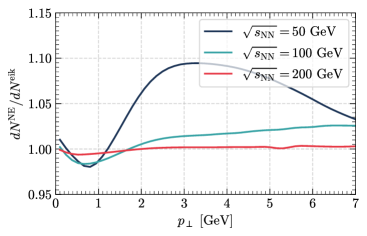
Figure 3: Ratio of the non-eikonal single inclusive gluon spectrum, Eq. (32), to the eikonal result ($\epsilon=0$) as a function of gluon transverse momentum, $p_{\perp}$, for three values of the center-of-mass energy per nucleon and for $\eta=0$.

In Fig. 4, we plot the same ratio as a function of the center-of-mass energy per nucleon for three values of pseudorapidity and for $p_{\perp}=2$ GeV. The results indicate that for $\eta=0$ the finite width effects are changing roughly between $10$ % to $3$ % up to between $\sqrt{s_{\rm NN}}\sim 40$ GeV to $\sqrt{s_{\rm NN}}\sim 100$ GeV, for $\eta=0.5$ they lead to up to $4$ % effect between $\sqrt{s_{\rm NN}}\sim 40$ GeV and $\sqrt{s_{\rm NN}}\sim 50$ GeV and for $\eta=1$ they are almost negligible. Note that even though the results are plotted starting from $\sqrt{s_{\rm NN}}=20$ GeV, at this low energy Bjorken-$x$ of the target parton probed by the projectile is $x\sim\frac{1\ {\rm GeV}}{\sqrt{s_{\rm NN}}}e^{-\eta}$, i.e., not small, and therefore our approach cannot not be considered reliable. Therefore, we consider our results starting from $\sqrt{s_{\rm NN}}\sim 40$ GeV where our approach is still valid.

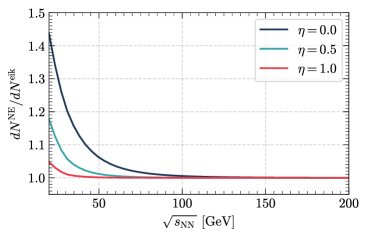
Figure 4: Ratio of the non-eikonal single gluon spectrum, given in Eq. (32), with respect to the eikonal one as a function of the center-of-mass energy per nucleon for three values of pseudorapidity and for $p_{\perp}=2$ GeV.

Finally, in Fig. 5, we plot the ratio as a function of the pseudorapidity of the produced gluon for three values of $\sqrt{s_{\rm NN}}$ and for $p_{\perp}=2$ GeV. The conclusions are analogous to the ones extracted from previous figures: the non-eikonal corrections yield to up to $\sim 6$ % effect for $\eta<1$ and when $\sqrt{s_{\rm NN}}=50$ GeV but it is almost negligible at higher energies at all values of the pseudorapidity.

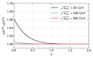
Figure 5: Ratio of the non-eikonal single gluon spectrum, given in Eq. (32), with respect to the eikonal one as a function of the pseudorapidity of the produced gluon for three values of $\sqrt{s_{\rm NN}}$ and for $p_{\perp}=2$ GeV.

4.3 Connection with earlier results in the literature

To finalize our study on the non-eikonal single inclusive gluon production, we make the explicit connection between our results and the ones obtained in Refs. Altinoluk:2014oxa ; Altinoluk:2015gia . We would like to emphasize that the results derived in this manuscript do not adopt any kind of expansion in the non-eikonal parameter $\epsilon^{2}$, and are therefore valid to all orders. On the other hand, in Refs. Altinoluk:2014oxa ; Altinoluk:2015gia a systematic expansion of the scalar propagator is proposed and the corrections are obtained up to next-to-next-to-eikonal accuracy. The expansion proposed in Refs. Altinoluk:2014oxa ; Altinoluk:2015gia for the scalar propagator is performed in two steps. First, an expansion of the scalar propagator around its classical trajectory, i.e., the one that minimizes the path integral and leads to a linear path instead of the Brownian motion. Then, a second geometric expansion by assuming that the angle between the classical trajectory and the longitudinal axis with constant transverse coordinate is small since it is proportional to $L^{+}/k^{+}$, and that the target field is weak far away from the classical solution. The corresponding result is an expansion in powers of $\frac{L^{+}}{k^{+}}=\frac{2i\epsilon^{2}}{Q_{s}^{2}}$. It is effectively performed for the function $\mathcal{R}_{\underline{k}}(L^{+},0;\textbf{y})$ which encodes the finite width target effects and is related to the scalar propagator via

$$\int_{\textbf{x}}e^{-i\textbf{k}\textbf{x}}\mathcal{G}_{k^{+}}(L^{+},\textbf{x};0,\textbf{y})=e^{-ik^{-}L^{+}}e^{-i\textbf{k}\textbf{y}}\mathcal{R}_{\underline{k}}(L^{+},0;\textbf{y}).$$ (48)

The result of the expansion at next-to-next-to-eikonal accuracy reads Altinoluk:2015gia

$$\mathcal{R}_{\underline{k}}(L^{+},0;\textbf{y})=U+\frac{2i\epsilon^{2}}{Q_{s}^{2}}\left[\textbf{k}^{i}U_{[0,1]}^{i}+\frac{i}{2}U_{[1,0]}\right]$$

$$\hskip 113.81102pt+\left(\frac{2i\epsilon^{2}}{Q_{s}^{2}}\right)^{2}\left[\textbf{k}^{i}\textbf{k}^{j}U_{[0,2]}^{ij}+\frac{i}{2}\textbf{k}^{i}U_{[1,1]}^{i}-\frac{1}{4}U_{[2,0]}\right]+\mathcal{O}\left(\epsilon^{6}\right),$$ (49)

where the color objects $U^{i\cdots j}_{[\alpha,\beta]}(L^{+},0;\textbf{y})$ are referred to as decorated Wilson lines. They can be identified with the non-eikonal partners of the standard Wilson lines.

In order to make the connection between the two results, one can immediately realize that the Fourier transform of the non-eikonal dipole functions that we have introduced in Eqs. (10) and (9) can be written in terms of $\mathcal{R}_{\underline{k}}(L^{+},0;\textbf{y})$ as

$$\int_{\textbf{x}}e^{-i\textbf{k}\cdot\textbf{x}}d^{(1)}(L^{+},0|{\mathbf{x}},{\mathbf{y}},k^{+};\bar{\mathbf{y}})=\frac{e^{-ik^{-}L^{+}}e^{-i\textbf{k}\cdot\mathbf{y}}}{(N_{c}^{2}-1)}\Big{\langle}{\rm Tr}\left[\mathcal{R}_{\underline{k}}(L^{+},0;\textbf{y})U_{\bar{\textbf{y}}}^{\dagger}(L^{+},0)\right]\Big{\rangle}_{T},$$ (50)

$$\int_{\textbf{x},\bar{\textbf{x}}}e^{-i\textbf{k}\cdot(\textbf{x}-\bar{\textbf{x}})}d^{(2)}(L^{+},0|{\mathbf{x}},{\mathbf{y}},k^{+};\bar{\mathbf{x}},\bar{\mathbf{y}},k^{+})$$

$$\hskip 142.26378pt=\frac{e^{-i\textbf{k}\cdot(\mathbf{y}-\mathbf{\bar{y}})}}{(N_{c}^{2}-1)}\Big{\langle}{\rm Tr}\left[\mathcal{R}_{\underline{k}}(L^{+},0;\textbf{y})\mathcal{R}^{\dagger}_{\underline{k}}(L^{+},0;\bar{\textbf{y}})\right]\Big{\rangle}_{T}.$$ (51)

Therefore, by using the non-eikonal expansion given in Eq. (4.3) we can write the Fourier transform of the $1^{\rm st}$ order NE dipole function as

$$e^{ik^{-}L^{+}+i\textbf{k}\cdot\mathbf{y}}\int_{\textbf{x}}e^{-i\textbf{k}\cdot\textbf{x}}d^{(1)}(L^{+},0|{\mathbf{x}},{\mathbf{y}},k^{+};\bar{\mathbf{y}})=\mathcal{O}(\textbf{r})+\frac{2i\epsilon^{2}}{Q_{s}^{2}}\left[\textbf{k}^{i}\mathcal{O}_{[0,1]}^{i}(\textbf{r})+\frac{i}{2}\mathcal{O}_{[1,0]}(\textbf{r})\right]$$

$$\hskip 85.35826pt+\left(\frac{2i\epsilon^{2}}{Q_{s}^{2}}\right)^{2}\left[\textbf{k}^{i}\textbf{k}^{j}\mathcal{O}_{[0,2]}^{ij}(\textbf{r})+\frac{i}{2}\textbf{k}^{i}\mathcal{O}_{[1,1]}^{i}(\textbf{r})-\frac{1}{4}\mathcal{O}_{[2,0]}(\textbf{r})\right]+\mathcal{O}\left(\epsilon^{6}\right),$$ (52)

where the tensors $\mathcal{O}^{i\cdots j;l\cdots m}_{[\alpha,\beta];[\gamma,\delta]}(\textbf{r})$ are referred to as decorated dipoles and are the leading eikonal corrections to the eikonal dipole function $\mathcal{O}(\textbf{r})=d^{(0)}(\mathbf{r})$. Furthermore, we note that in order to write Eq. (4.3), we assume translational invariance of the decorated dipoles and write $\mathbf{r}=\mathbf{y}-\mathbf{\bar{y}}$. The definitions of these dipole functions are:

$$\mathcal{O}(\textbf{r}) =\frac{1}{N_{c}^{2}-1}\Big{\langle}{\rm Tr}\left[U_{{\textbf{y}}}(L^{+},0)U_{\bar{\textbf{y}}}^{\dagger}(L^{+},0)\right]\Big{\rangle}_{T},$$ (53)

$$\mathcal{O}^{i\cdots j}_{[\alpha,\beta]}(\textbf{r}) =\frac{1}{N_{c}^{2}-1}\Big{\langle}{\rm Tr}\left[U^{i\cdots j}_{[\alpha,\beta]}(L^{+},0;\textbf{y})U_{\bar{\textbf{y}}}^{\dagger}(L^{+},0)\right]\Big{\rangle}_{T},$$ (54)

$$\mathcal{O}^{i\cdots j;l\cdots m}_{[\alpha,\beta];[\gamma,\delta]}(\textbf{r}) =\frac{1}{N_{c}^{2}-1}\Big{\langle}{\rm Tr}\left[U^{i\cdots j}_{[\alpha,\beta]}(L^{+},0;\textbf{y})U^{l\cdots m\dagger}_{[\gamma,\delta]}(L^{+},0;\bar{\textbf{y}})\right]\Big{\rangle}_{T}.$$ (55)

On the other hand, the Fourier transform of the $2^{\rm nd}$ order NE dipole function can be written in the same fashion, reading

$$e^{i\textbf{k}\cdot(\mathbf{y}-\mathbf{\bar{y}})}\int_{\textbf{x},\bar{\textbf{x}}}e^{-i\textbf{k}\cdot(\textbf{x}-\bar{\textbf{x}})}d^{(2)}(L^{+},0|{\mathbf{x}},{\mathbf{y}},k^{+};\bar{\mathbf{x}},\bar{\mathbf{y}},k^{+})$$

$$\hskip 28.45274pt=\mathcal{O}(\textbf{r})+\frac{2i\epsilon^{2}}{Q_{s}^{2}}\left[\textbf{k}^{i}\left(\mathcal{O}^{i}_{[0,1]}(\textbf{r})+\mathcal{O}^{i}_{[0,1]}(-\textbf{r})\right)+\frac{i}{2}\left(\mathcal{O}_{[1,0]}(\textbf{r})-\mathcal{O}_{[1,0]}(-\textbf{r})\right)\right]$$

$$\hskip 28.45274pt+\left(\frac{2i\epsilon^{2}}{Q_{s}^{2}}\right)^{2}\Bigg{[}\textbf{k}^{i}\textbf{k}^{j}\Big{(}\mathcal{O}^{ij}_{[0,2]}(\textbf{r})+\mathcal{O}^{ij}_{[0,2]}(-\textbf{r})+\mathcal{O}^{ij}_{[0,1];[0,1]}(\textbf{r})\Big{)}$$

$$\hskip 85.35826pt+\textbf{k}^{i}\frac{i}{2}\Big{(}\mathcal{O}^{i}_{[1,1]}(\textbf{r})-\mathcal{O}^{i}_{[1,1]}(-\textbf{r})+\mathcal{O}^{i}_{[1,0];[0,1]}(\textbf{r})-\mathcal{O}^{i}_{[1,0];[0,1]}(-\textbf{r})\Big{)}$$

$$\hskip 128.0374pt-\frac{1}{4}\Big{(}\mathcal{O}_{[2,0]}(\textbf{r})-\mathcal{O}_{[2,0]}(-\textbf{r})+\mathcal{O}_{[1,0];[1,0]}(\textbf{r})\Big{)}\Bigg{]}+\mathcal{O}\left(\epsilon^{6}\right).$$ (56)

We can now make a one-to-one comparison between our result Eqs.  (4.1) and (4.3) (and also between Eqs. (35) and (4.3)) by expanding our results to the appropriate order in order to obtain a parametrization of the decorated dipoles within the GBW model, i.e., assuming a Gaussian form. Expanding the Fourier transform of the $1^{\rm st}$ order NE dipole function given in Eq. (4.1) at next-to-next-to-eikonal accuracy, i.e., in terms of $\epsilon^{2}$ up to order $\epsilon^{4}$, we get

$$e^{ik^{-}L^{+}+i\textbf{k}\cdot\mathbf{y}}\int_{\textbf{x}}e^{-i\textbf{k}\cdot\textbf{x}}d^{(1)}(L^{+},0|{\mathbf{x}},{\mathbf{y}},k^{+};\bar{\mathbf{y}})$$

$$\hskip-14.22636pt=e^{-\frac{Q_{s}^{2}}{4}\mathbf{r}^{2}}\Bigg{\{}1-\frac{2i\epsilon^{2}}{Q_{s}^{2}}\frac{Q_{s}^{2}}{4}\Bigg{[}\mathbf{k}^{i}\mathbf{r}^{i}-i\left(\frac{Q_{s}^{2}}{6}\mathbf{r}^{2}-1\right)\Bigg{]}+\left(\frac{2i\epsilon^{2}}{Q_{s}^{2}}\right)^{2}\Bigg{[}\textbf{k}^{i}\textbf{k}^{j}\left(\frac{Q_{s}^{4}}{32}\textbf{r}^{i}\textbf{r}^{j}-\frac{Q_{s}^{2}}{12}\delta^{ij}\right)$$

$$\hskip 28.45274pt-i\textbf{k}^{i}\textbf{r}^{i}Q_{s}^{4}\left(\frac{11}{96}+\frac{Q_{s}^{2}}{96}\textbf{r}^{2}\right)+Q_{s}^{4}\left(-\frac{5}{96}+\frac{3}{160}Q_{s}^{2}\textbf{r}^{2}-\frac{Q_{s}^{4}}{1152}\textbf{r}^{4}\right)\Bigg{]}\Bigg{\}}+{\cal O}(\epsilon^{6}).$$ (57)

A term by term comparison of Eqs. (4.3) and (4.3) leads to the following parametrization of the decorated dipoles in our Gaussian ansatz:

$$\mathcal{O}(\textbf{r}) =e^{-\frac{Q_{s}^{2}}{4}\textbf{r}^{2}},$$ (58)

$$\mathcal{O}_{[0,1]}^{i}(\textbf{r}) =-\frac{Q_{s}^{2}}{4}\textbf{r}^{i}e^{-\frac{Q_{s}^{2}}{4}\textbf{r}^{2}},$$ (59)

$$\mathcal{O}_{[1,0]}(\textbf{r}) =\frac{Q_{s}^{2}}{12}\left(-6+Q_{s}^{2}\textbf{r}^{2}\right)e^{-\frac{Q_{s}^{2}}{4}\textbf{r}^{2}},$$ (60)

$$\mathcal{O}_{[0,2]}^{ij}(\textbf{r}) =\frac{Q_{s}^{2}}{4}\left(-\frac{1}{3}\delta^{ij}+\frac{Q_{s}^{2}}{8}\textbf{r}^{i}\textbf{r}^{j}\right)e^{-\frac{Q_{s}^{2}}{4}\textbf{r}^{2}},$$ (61)

$$\mathcal{O}_{[1,1]}^{i}(\textbf{r}) =-\frac{Q_{s}^{4}}{48}\textbf{r}^{i}\left(11+Q_{s}^{2}\textbf{r}^{2}\right)e^{-\frac{Q_{s}^{2}}{4}\textbf{r}^{2}},$$ (62)

$$\mathcal{O}_{[2,0]}(\textbf{r}) =\frac{Q_{s}^{4}}{8}\left(\frac{5}{3}-\frac{3}{5}Q_{s}^{2}\textbf{r}^{2}+\frac{1}{36}Q_{s}^{4}\textbf{r}^{4}\right)e^{-\frac{Q_{s}^{2}}{4}\textbf{r}^{2}}.$$ (63)

On the other hand, by using Eq. (35), the Fourier transform of the $2^{\rm nd}$ order NE dipole function can be written as

$$e^{i\textbf{k}\cdot(\mathbf{y}-\mathbf{\bar{y}})}\int_{\textbf{x},\bar{\textbf{x}}}e^{-i\textbf{k}\cdot(\textbf{x}-\bar{\textbf{x}})}d^{(2)}(L^{+},0|{\mathbf{x}},{\mathbf{y}},k^{+};\bar{\mathbf{x}},\bar{\mathbf{y}},k^{+})=e^{-\frac{1}{4}Q_{s}^{2}\textbf{r}^{2}}.$$ (64)

As mentioned earlier, the $2^{\rm nd}$ order NE dipole function does not encode any finite width effect in the case in where both longitudinal momenta are equal and therefore it is of $\mathcal{O}(\epsilon^{0})$. Thus, comparing Eqs. (4.3) and (64) and keeping in mind that the non-eikonal corrections in Eq. (4.3) vanish in the Gaussian approximation, we obtain the following constraints for the decorated dipoles:

$$\mathcal{O}^{ij}_{[0,1];[0,1]}(\textbf{r}) =-2\mathcal{O}^{ij}_{[0,2]}(\textbf{r}),$$ (65)

$$\mathcal{O}^{i}_{[1,0];[0,1]}(\textbf{r})-\mathcal{O}^{i}_{[1,0];[0,1]}(-\textbf{r}) =-2\mathcal{O}^{i}_{[1,1]}(\textbf{r}),$$ (66)

$$\mathcal{O}_{[1,0];[1,0]}(\textbf{r}) =2\mathcal{O}_{[2,0]}(\textbf{r}).$$ (67)

We conclude that by comparing the model independent non-eikonal expansion given in Refs. Altinoluk:2014oxa ; Altinoluk:2015gia with our approach, which relies on the Gaussian form of the dipole functions, we are able to obtain a parameterization of the decorated dipoles in the Gaussian ansatz that is valid for small size dipoles. This parameterization may be useful for including finite target width effects in future phenomenological studies.

5 Non-eikonal multigluon production

In this section we study the general case that corresponds to the non-eikonal $n$-gluon production whose generic expression is given in Eq. (2). Throughout this study, we adopt the Area Enhancement approximation in order to write the multipoles as non-eikonal two point functions (or dipoles). The validity of the AE argument when the finite width target effects are included in the computation is discussed at the end of Section 3. We would like to also mention that in Ref. Agostini:2021xca we investigated multigluon production in the strict eikonal limit where we introduced a diagramatic approach to study the $2n$-point correlators within the AE argument. Our aim, in this section, is to generalize that approach to the non-eikonal case where the finite longitudinal width of the target is accounted for.

Let us start by writing the $n$-gluon spectrum given in Eq. (2) in terms of the simplified notations introduced in Ref. Agostini:2021xca . Within the AE model, the non-eikonal $n$-gluon spectra can be written as

$$\frac{d^{n}N}{\prod_{i=1}^{n}d\eta_{2i-1}d^{2}\textbf{k}_{2i-1}}=\frac{1}{2^{n}(2\pi)^{3n}} \int\left(\prod_{i=1}^{2n}\frac{d^{2}\textbf{q}_{i}}{(2\pi)^{2}}\right)\left(\sum_{\sigma\in\Pi(\chi)}\prod_{\{i,j\}\in\sigma}\Big{\langle}\Omega_{i}\Omega_{j}\Big{\rangle}_{p}\right)$$

$$\hskip 85.35826pt\times\left(\sum_{\omega\in\Pi(\chi)}\prod_{\{\alpha,\beta\}\in\omega}\Big{\langle}\Lambda_{\alpha}\Lambda_{\beta}\Big{\rangle}_{T}\right),$$ (68)

where $\chi=\{1,2,\dots,2n\}$ represents the total number of color charges in the amplitude and in the complex conjugate amplitude (i.e., on both sides of the cut) and $\Pi(\chi)$ represents the set of partitions of $\chi$ with disjoint pairs. The projectile is represented by function $\Omega_{i}$ which is given by

$$\Omega_{i}=g\rho^{b_{i}}(\mathbf{q}_{i}),$$ (69)

with the property that for odd $i$ the color source sits on the left side of the cut and for even $i$ it sits on the right side. The two point correlator of the function $\Omega_{i}$ is defined as

$$\Big{\langle}\Omega_{i}\Omega_{j}\Big{\rangle}_{p}=\frac{\delta^{b_{i}b_{j}}}{N_{c}^{2}-1}\mu_{p}^{2}\big{(}(-1)^{i+1}\textbf{q}_{i},(-1)^{j+1}\textbf{q}_{j}\big{)},\quad\mu_{p}^{2}(\mathbf{k},\mathbf{q})=\pi B_{p}e^{-\frac{(\mathbf{k}+\mathbf{q})^{2}}{4}B_{p}}.$$ (70)

On the other hand, the object $\Lambda_{\alpha}$ represents the target and its interaction with the projectile. It is defined as

$$\Lambda_{\alpha}=\overline{{\cal M}}^{a_{\alpha}b_{\alpha}}_{\lambda_{\alpha}}({\underline{k}}_{\alpha},\mathbf{q}_{\alpha}),$$ (71)

with odd values of $\alpha$ corresponding to the left side of the cut and even values of $\alpha$ to the right side of the cut. Therefore, for even values of $\alpha$ one takes the complex conjugate of the reduced amplitude.

Similar to the strict eikonal case, we impose the following constraints on the produced gluons:

$${\underline{k}}_{2n} ={\underline{k}}_{2n-1},$$ (72)

$$a_{2n} =a_{2n-1},$$ (73)

$$\lambda_{2n} =\lambda_{2n-1},$$ (74)

namely the color, polarization and both transverse and longitudinal momenta of the produced gluons have to be the same on both sides of the cut. We would like to remind that the arguments introduced at the end of Section 3 to justify the use of AE model in the non-eikonal case where the finite longitudinal width effects are accounted for, are based on the fact that the fluctuation time of the target fields is much larger than its longitudinal extent. This implies that that chromo-electric domains do not decohere during the interaction of the projectile and the target. Moreover, it also allows one to argue that each domain has to be color neutral and the target average has to be a singlet. Therefore, we can write the two point correlators of functions $\Lambda_{\alpha}$ as

$$\Big{\langle}\Lambda_{\alpha}\Lambda_{\beta}\Big{\rangle}_{T}=\frac{\delta^{a_{\alpha}a_{\beta}}\delta^{b_{\alpha}b_{\beta}}}{(N_{c}^{2}-1)^{2}}\Big{\langle}\text{Tr}\left[\overline{{\cal M}}_{\lambda_{\alpha}}({\underline{k}}_{\alpha},\mathbf{q}_{\alpha})\overline{{\cal M}}_{\lambda_{\beta}}({\underline{k}}_{\beta},\mathbf{q}_{\beta})\right]\Big{\rangle}_{T}.$$ (75)

Using the definition of the reduced amplitude given in Eq. (2), and the definitions of the eikonal and non-eikonal dipole functions introduced in Eqs. (10), (9) and (8), the 2-point correlator becomes

$$\Big{\langle}\Lambda_{\alpha}\Lambda_{\beta}\Big{\rangle}_{T}=\frac{\delta^{a_{\alpha}a_{\beta}}\delta^{b_{\alpha}b_{\beta}}}{N_{c}^{2}-1}(2\pi)^{2}\delta^{(2)}\big{[}\pm(\mathbf{k}_{\alpha}-\mathbf{q}_{\alpha})+\pm(\mathbf{k}_{\beta}-\mathbf{q}_{\beta})\big{]}$$

$$\hskip 0.0pt\times\Bigg{\{}2\frac{\mathbf{k}_{\alpha}^{\lambda_{\alpha}}\mathbf{k}_{\beta}^{\lambda_{\beta}}}{\mathbf{k}_{\alpha}^{2}\mathbf{k}_{\beta}^{2}}I_{\rm aft-aft}\big{(}\mathbf{k}_{\beta},\mathbf{q}_{\beta}\big{)}-4\frac{\mathbf{k}_{\alpha}^{\lambda_{\alpha}}\mathbf{q}_{\beta}^{\lambda_{\beta}}}{\mathbf{k}_{\alpha}^{2}\mathbf{q}_{\beta}^{2}}I_{\rm aft-bef}\Big{(}\mathbf{k}_{\beta},\mathbf{q}_{\beta},\pm k_{\beta}^{+}\Big{)}$$

$$\hskip 0.0pt+2\frac{\mathbf{q}_{\alpha}^{\lambda_{\alpha}}\mathbf{q}_{\beta}^{\lambda_{\beta}}}{\mathbf{q}_{\alpha}^{2}\mathbf{q}_{\beta}^{2}}I_{\rm bef-bef}\Big{(}\pm\mathbf{k}_{\alpha},\pm\mathbf{q}_{\alpha},\pm\mathbf{k}_{\beta},\pm\mathbf{q}_{\beta};\pm k_{\alpha}^{+},\pm k_{\beta}^{+}\Big{)}$$

$$\hskip 0.0pt+2\frac{L^{+}}{k_{\beta}^{+}}\frac{\mathbf{k}_{\alpha}^{\lambda_{\alpha}}}{\mathbf{k}_{\alpha}^{2}}\int_{0}^{1}df_{\beta}I^{\lambda_{\beta}}_{\rm aft-in}\Big{(}\pm\mathbf{k}_{\beta},\pm\mathbf{q}_{\beta},\pm k_{\beta}^{+};f_{\beta}\Big{)}$$

$$\hskip 0.0pt-2\frac{L^{+}}{k_{\beta}^{+}}\frac{\mathbf{q}_{\alpha}^{\lambda_{\alpha}}}{\mathbf{q}_{\alpha}^{2}}\int_{0}^{1}df_{\beta}I^{\lambda_{\beta}}_{\rm in-bef}\Big{(}\pm\mathbf{k}_{\alpha},\pm\mathbf{q}_{\alpha},\pm\mathbf{k}_{\beta},\pm\mathbf{q}_{\beta};\pm k_{\alpha}^{+},\pm k_{\beta}^{+};f_{\beta}\Big{)}$$

$$\hskip 0.0pt+\frac{L^{+}}{k_{\alpha}^{+}}\frac{L^{+}}{k_{\beta}^{+}}\int_{0}^{1}df_{\beta}\int_{0}^{f_{\beta}}df_{\alpha}I^{\lambda_{\alpha}\lambda_{\beta}}_{\rm in-in}\Big{(}\pm\mathbf{k}_{\alpha},\pm\mathbf{k}_{\beta},\pm\mathbf{q}_{\beta};\pm k_{\alpha}^{+},\pm k_{\beta}^{+};f_{\alpha},f_{\beta}\Big{)}$$

$$\hskip 0.0pt+(\alpha\leftrightarrow\beta)\Bigg{\}},$$ (76)

where we have introduced the notation $\pm k_{a}\equiv(-1)^{a+1}k_{a}$. It corresponds to stating that when the respective momentum (either longitudinal or transverse) is on the left side of the cut, i.e., with $a$ odd, it is multiplied by $(+1)$ and when it is on the right side it is multiplied by $(-1)$, changing its sign due to the Fourier transform. The explicit expressions for the functions $I$ are given in Appendix B.

Thus, in order to compute the $n$-gluon spectra, one needs to evaluate the Wick expansions given in Eq. (5). On the projectile side, since we are adopting the MV model for the projectile configurations, projectile averages factorize into 2-point correlators defined in Eq. (70). On the target side, we are using the AE model to perform the averages over the target fields which also factorize into 2-point correlators of the reduced matrix amplitudes, given in Eq. (5). Expanding the $\left(\frac{(2n)!}{2^{n}n!}\right)^{2}$ terms in Eq. (5) and evaluating the 2-point correlators (on both the projectile and the target sides), we are able to compute the $n$-gluon spectra for any value of $n$ neglecting, of course, contributions that are subleading in powers of $\rho_{p}$. Since multigluon spectra contain a very large number of terms, it is convenient to use the diagrammatic approach introduced in Ref. Agostini:2021xca .

Finally, let us note that the single inclusive gluon spectrum can be computed in the approach presented in this section by just writing

$$\frac{dN}{d\eta d^{2}\mathbf{k}}=\frac{g^{2}}{2(2\pi)^{3}}\int_{\mathbf{q}_{1},\mathbf{q}_{2}}\Big{\langle}\Omega_{1}\Omega_{2}\Big{\rangle}_{p}\Big{\langle}\Lambda_{1}\Lambda_{2}\Big{\rangle}_{T}.$$ (77)

It is straightforward to see that if we use Eqs. (70) and (5), this equation reduces to Eq. (32). In the next subsection, we study the double inclusive gluon production by using the setup introduced here.

5.1 Non-eikonal double inclusive gluon production

Now we focus on the non-eikonal double inclusive gluon production – the $n=2$ case in the multigluon spectrum in Eq. (5). In our set up, the double inclusive spectrum reads

$$\frac{d^{2}N}{d\eta_{1}d^{2}\mathbf{k}_{1}d\eta_{3}d^{2}\mathbf{k}_{3}}=\frac{g^{4}}{4(2\pi)^{6}}\int_{\mathbf{q}_{1},\mathbf{q}_{2},\mathbf{q}_{3},\mathbf{q}_{4}}$$

$$\hskip 56.9055pt\times\Bigg{(}\Big{\langle}\Omega_{1}\Omega_{2}\Big{\rangle}_{p}\Big{\langle}\Omega_{3}\Omega_{4}\Big{\rangle}_{p}+\Big{\langle}\Omega_{1}\Omega_{3}\Big{\rangle}_{p}\Big{\langle}\Omega_{2}\Omega_{4}\Big{\rangle}_{p}+\Big{\langle}\Omega_{1}\Omega_{4}\Big{\rangle}_{p}\Big{\langle}\Omega_{2}\Omega_{3}\Big{\rangle}_{p}\Bigg{)}$$

$$\hskip 56.9055pt\times\Bigg{(}\Big{\langle}\Lambda_{1}\Lambda_{2}\Big{\rangle}_{T}\Big{\langle}\Lambda_{3}\Lambda_{4}\Big{\rangle}_{T}+\Big{\langle}\Lambda_{1}\Lambda_{3}\Big{\rangle}_{T}\Big{\langle}\Lambda_{2}\Lambda_{4}\Big{\rangle}_{T}+\Big{\langle}\Lambda_{1}\Lambda_{4}\Big{\rangle}_{T}\Big{\langle}\Lambda_{2}\Lambda_{3}\Big{\rangle}_{T}\Bigg{)},$$ (78)

where the 2-point functions for the projectile and the target sides are given by Eqs. (70) and (5) respectively.

Double inclusive gluon production has been studied extensively in the eikonal approximation (see Refs. Dumitru:2008wn ; Dumitru:2010iy ; Kovchegov:2012nd ; Kovchegov:2013ewa ; Altinoluk:2015uaa ; Altinoluk:2015eka ; Altinoluk:2016vax ). In the eikonal limit, double inclusive gluon production spectrum contains not only a fully uncorrelated piece, but also Bose Enhancement and Hanbury-Brown-Twiss-like (HBT) correlations encoded in the terms that are suppressed by powers of $(N_{c}^{2}-1)$ with respect to the fully uncorrelated one. Moreover, it has been shown that the eikonal results give non-zero even harmonics but vanishing odd harmonics. This is due to an accidental symmetry of the CGC which is encoded in the double inclusive spectrum through its $\mathbf{k}_{3}\to-\mathbf{k}_{3}$ symmetry, with ${\mathbf{k}}_{3}$ being the transverse momenta of the second gluon. Over the last decade, there have been many suggested ways to break this symmetry (see Ref. Altinoluk:2020wpf for a review). One of the ways to break this symmetry and generate non-zero odd harmonics through CGC calculations is to include non-eikonal corrections, as has been shown in Refs. Agostini:2019avp ; Agostini:2019hkj for proton-proton collisions.

The non-eikonal double inclusive spectrum given in Eq. (5.1) resembles its eikonal limit in many features. First, the term proportional to $\big{\langle}\Omega_{1}\Omega_{2}\big{\rangle}_{p}\big{\langle}\Omega_{3}\Omega_{4}\big{\rangle}_{p}\big{\langle}\Lambda_{1}\Lambda_{2}\big{\rangle}_{T}\big{\langle}\Lambda_{3}\Lambda_{4}\big{\rangle}_{T}$ is the fully uncorrelated piece and it is the leading term in the $N_{c}$ counting. Bose Enhancement and HBT-like correlations are encoded in the other terms in Eq. (5.1) and they are subleading in powers of $(N_{c}^{2}-1)$ and collision area (actually in $B_{p}Q_{s}^{2}$) just as in its eikonal limit. The main difference between the non-eikonal double inclusive spectrum given in Eq. (5.1) and its eikonal limit is that the non-eikonal corrections break the accidental symmetry of the CGC. Note that Eq. (5.1) is symmetric under the exchange of $({\underline{k}}_{3}\to-{\underline{k}}_{3})$ where ${\underline{k}}_{3}\equiv(k_{3}^{+},{\mathbf{k}}_{3})$, but not under $\mathbf{k}_{3}\to-\mathbf{k}_{3}$. Therefore, non-eikonal corrections introduce an asymmetry in the spectrum with respect to the azimuthal angle.

In order to see this asymmetry explicitly, we compute the non-eikonal double inclusive gluon spectrum given in Eq. (5.1) numerically. For that purpose, we need to expand the terms inside the parenthesis in Eq. (5.1) and use Eqs. (70) and (5) as the definitions of the 2-point correlators for the projectile and the target averages respectively. Similar to the treatment in the single inclusive case, the infrared divergences that appear in the limit $\mathbf{q}_{i}\to 0$ in Eq. (5) are regulated by introducing a mass term $m^{2}$ in the denominators, i.e., we perform the change $1/\mathbf{q}_{i}^{2}\to 1/(\mathbf{q}_{i}^{2}+m^{2})$, where the value of the regulator is fixed to $m=0.4$ GeV. We also fix in the numerical evaluations $N_{c}=3$, $A^{1/3}=6$, $B_{p}=6$ GeV^-2 and $Q_{s}^{2}=2$ GeV².

The results are presented in Fig. 6, where we plot the solution of Eq. (5.1) and its respective eikonal limit as a function of the azimuthal angle $\Delta\phi=\arccos\frac{\mathbf{k}_{1}\cdot\mathbf{k}_{3}}{|\mathbf{k}_{1}||\mathbf{k}_{3}|}$. In this plot, we used $\sqrt{s_{\rm NN}}=100$ GeV, $\eta_{1}=\eta_{3}=0.2$ and $|\mathbf{k}_{1}|=|\mathbf{k}_{3}|=1$ GeV. As discussed above, a clear asymmetry between the near- and away-side peaks appears in the non-eikonal double gluon spectrum. This observation confirms the breaking of the accidental symmetry of the CGC by introducing the non-eikonal corrections that here we check in the dilute-dense ($pA$) situation. Moreover, Fig. 6 shows that the non-eikonal spectrum differs from the eikonal one by $4\%$ in the near-side and $8\%$ in the away-side peak. In this kinematics, this is a slightly larger correction than the one in the single inclusive spectrum discussed in Section 4.2.

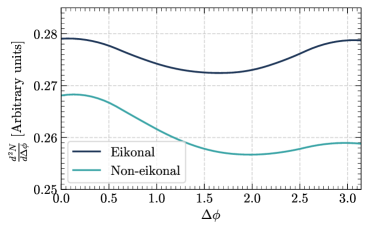
Figure 6: The double inclusive gluon spectrum given in Eq. (5.1) and its eikonal limit as a function of the azimuthal angle $\Delta\phi$. In this plot, we have fixed $\sqrt{s_{\rm NN}}=100$ GeV, $\eta_{1}=\eta_{3}=0.2$ and $|\mathbf{k}_{1}|=|\mathbf{k}_{3}|=1$ GeV.

These results clearly indicate that non-eikonal corrections provide non-vanishing odd harmonics since the accidental symmetry of the CGC is broken by their inclusion. We leave a detailed analysis of the azimuthal harmonics for a future work.

6 Conclusions and Outlook

In this work we generalized to proton-nucleus collisions the framework proposed in Refs. Agostini:2019avp ; Agostini:2019hkj for proton-proton collisions. We computed multigluon spectra including the non-eikonal corrections that stem from the finite longitudinal width of the target. We use the Area Enhancement model that allows for an expansion of multipoles in terms of dipoles by neglecting contributions suppressed by powers of the overlap area of projectile and target. The formalism adopted in this work is inspired by the one used in jet quenching studies Casalderrey-Solana:2007knd ; Mehtar-Tani:2013pia ; Blaizot:2015lma where a non-zero longitudinal extent of the dense medium is essential to study parton propagation in the Quark Gluon Plasma. We adopt and extend such formalism to compute particle production and correlations in the Color Glass Condensate for the first time, where the effect of considering a finite medium width is small as compared to the jet quenching case where this is the main contribution to emission processes.

We have shown that the non-eikonal corrections in the target 2-point correlators can be computed analytically using the GBW approximation that assumes that the eikonal dipole function has a Gaussian form. This approximation is justified as long as the dipole size is $\ll\Lambda_{\rm QCD}^{-1}$. The results for the non-eikonal dipole functions are given in Eqs. (11), (21) and (3), where the finite width target effects are accounted for, encoded in the dimensionless non-eikonal parameter $\epsilon^{2}=\frac{Q_{s}^{2}L^{+}}{2ik^{+}}$. Using these results, we computed the single inclusive gluon spectrum beyond eikonal accuracy. The results of the single inclusive gluon production are summarized in Figs. 3, 4 and 5. They show that including the non-eikonal corrections to the single inclusive gluon spectrum results in between $2$ % to $10$ % effect for center-of-mass energies per nucleon smaller than 100 GeV and for pseudorapidities of the produced particle smaller than 1. Thus, we conclude that the non-eikonal corrections are not sizable for phenomenological studies in single inclusive gluon production at top RHIC or LHC energies. In Section 4.3, we compare the next-to-next-to-eikonal approximation of our results, i.e., an expansion up to order $\epsilon^{4}$, with the one presented in Altinoluk:2014oxa ; Altinoluk:2015gia . We obtained a parameterization of the so-called decorated dipoles within the Gaussian ansatz that we have used here.

In Section 5 we generalize the framework introduced in Agostini:2021xca to compute multigluon production, to the non-eikonal case where the corrections to the eikonal approximation stem from the finite longitudinal with of the target. Like in its eikonal limit, our framework is based on the Area Enhancement model that we argue should be valid for a target with finite longitudinal size since the coherence length of the chromo-electric domains is much larger than the longitudinal extent of the target. We then focused on double inclusive gluon production and performed its numerical analysis (see Fig. 6). The results suggest two important outcomes. First, for not very high energies and rapidities, the non-eikonal corrections to the double inclusive gluon spectrum are slightly larger than those to the single inclusive case. Second, the non-eikonal corrections induce an azimuthal asymmetry in the double inclusive spectrum which demonstrates that the inclusion of such corrections breaks the accidental symmetry of the CGC, as in $pp$ Agostini:2019avp ; Agostini:2019hkj . Therefore, we expect to obtain non-vanishing odd harmonics from the non-eikonal double inclusive gluon spectrum in $pA$ collisions. A detailed study of the effects of non-eikonal corrections to both even and odd azimuthal harmonics demands a dedicated numerical effort that we leave for the future.

Appendix A Harmonic oscillator path integrals

In this section we compute solve the path integrals that appear in Section 3. Before starting our discussion we define the following matrix:

$$[F_{N}(x)]_{ij}=\begin{cases}x&\text{if $i=j$},\\ -1&\text{if $|i-j|=1$},\\ 0&\text{otherwise},\end{cases}$$ (79)

with $x$ a positive real scalar and $i,j=1,\dots,N$. Therefore $F_{N}$ is a $N\times N$ tridiagonal matrix with $x$ in the main diagonal and $-1$ in the neighbour diagonals. Since this matrix will be a key ingredient in the calculation of this section we will study some of its properties.

By performing the Laplace expansion of this matrix it is easy to see that it follows the following recursive equation:

$$\det F_{N}(x)=x\det F_{N-1}(x)-\det F_{N-2}(x).$$ (80)

The solution of this equation is

$$\det F_{N}(x)=\frac{2^{-(N+1)}}{\sqrt{x^{2}-4}}\left(x_{+}^{N+1}-x_{-}^{N+1}\right),$$ (81)

where $x_{\pm}=x\pm\sqrt{x^{2}-4}$.

The inverse of $F_{N}(x)$ can be computed by using the expression of the inverse of a block matrix:

$$\begin{pmatrix}\mathbf{A}&\mathbf{B}\\ \mathbf{C}&\mathbf{D}\end{pmatrix}^{-1} =\begin{pmatrix}\left(\mathbf{A}-\mathbf{BD}^{-1}\mathbf{C}\right)^{-1}&-\left(\mathbf{A}-\mathbf{BD}^{-1}\mathbf{C}\right)^{-1}\mathbf{BD}^{-1}\\ -\mathbf{D}^{-1}\mathbf{C}\left(\mathbf{A}-\mathbf{BD}^{-1}\mathbf{C}\right)^{-1}&\quad\mathbf{D}^{-1}+\mathbf{D}^{-1}\mathbf{C}\left(\mathbf{A}-\mathbf{BD}^{-1}\mathbf{C}\right)^{-1}\mathbf{BD}^{-1}\end{pmatrix}$$

$$\hskip-28.45274pt=\begin{pmatrix}\mathbf{A}^{-1}+\mathbf{A}^{-1}\mathbf{B}\left(\mathbf{D}-\mathbf{CA}^{-1}\mathbf{B}\right)^{-1}\mathbf{CA}^{-1}&-\mathbf{A}^{-1}\mathbf{B}\left(\mathbf{D}-\mathbf{CA}^{-1}\mathbf{B}\right)^{-1}\\ -\left(\mathbf{D}-\mathbf{CA}^{-1}\mathbf{B}\right)^{-1}\mathbf{CA}^{-1}&\left(\mathbf{D}-\mathbf{CA}^{-1}\mathbf{B}\right)^{-1}\end{pmatrix}.$$ (82)

Noting that $F_{N}(x)$ can be written as a block matrix with $\mathbf{A}=x$, $\mathbf{D}=F_{N-1}(x)$, $\mathbf{C}_{i}=-\delta_{i,2}$ and $\mathbf{B}_{j}=-\delta_{j,2}$, we can compute the inverse of its component $(1,1)$ by using the first equality of (A):

$$[F^{-1}_{N}(x)]_{1,1}=\Big{(}x-[F^{-1}_{N-1}(x)]_{1,1}\Big{)}^{-1}.$$ (83)

Analogously, we could use the second equality of (A) with $\mathbf{A}=F_{N-1}(x)$, $\mathbf{D}=x$, $\mathbf{C}_{j}=-\delta_{j,N-1}$ and $\mathbf{B}_{i}=-\delta_{i,N-1}$ to obtain the same recursive equation for $[F_{N}(x)^{-1}]_{N,N}$. Solving (83) we obtain

$$[F_{N}^{-1}(x)]_{1,1}=[F_{N}^{-1}(x)]_{N,N}=\frac{2^{-N}}{\sqrt{x^{2}-4}\det F_{N}(x)}\left(x_{+}^{N}-x_{-}^{N}\right).$$ (84)

Inspecting (A), we realize that the rest of the components of $F_{N}^{-1}(x)$ can be computed just as a function of its $(1,1)$ and $(N,N)$ components. In this manuscript we will only need the $(1,N)$ and $(N,1)$ components of this matrix which can be written

$$[F_{N}^{-1}(x)]_{1,N}=[F_{N}^{-1}(x)]_{N,1}=\frac{1}{\det F_{N}(x)}\ .$$ (85)

We now proceed to solve the path integrals. The first path integral that we encounter in Section 3 is the one of a single harmonic oscillator of mass $m$ and coupling $\kappa$:

$$\int_{\textbf{y}}^{\textbf{x}}\left[\mathcal{D}\textbf{z}\right]{\rm exp}\left\{\int_{y^{+}}^{x^{+}}dz^{+}\left[m\dot{\textbf{z}}^{2}-\kappa\textbf{z}^{2}\right]\right\},$$ (86)

where, from (20), $m=\frac{ik^{+}}{2}$ and $\kappa=\frac{Q_{s}^{2}}{4L^{+}}$. By discretizing the longitudinal direction into $N$ slices we can write this equation as

$$\lim_{N\rightarrow\infty}\int\left(\prod_{n=1}^{N-1}d^{2}\textbf{z}_{n}\right)\left(\frac{-mN}{\pi\Delta^{+}}\right)^{N}{\rm exp}\left\{\sum_{n=1}^{N}\left[\frac{mN}{\Delta^{+}}(\textbf{z}_{n}-\textbf{z}_{n-1})^{2}-\frac{\kappa\Delta^{+}}{N}\textbf{z}_{n}^{2}\right]\right\}$$

$$\hskip 0.0pt=\lim_{N\rightarrow\infty}\int\left(\prod_{n=1}^{N-1}d^{2}\textbf{z}_{n}\right)\left(\frac{a}{2\pi}\right)^{N}{\rm exp}\left\{\sum_{n=1}^{N}\left[-\frac{a}{2}(\textbf{z}_{n}-\textbf{z}_{n-1})^{2}-b\textbf{z}_{n}^{2}\right]\right\},$$ (87)

where we have defined $\Delta^{+}=x^{+}-y^{+}$ and

$$a=-\frac{2mN}{\Delta^{+}}\ ,\qquad b=\frac{\kappa\Delta^{+}}{N}\ .$$ (88)

In order to solve this integral it is convenient to write it in a matrix form. In order to do so we define the vector $\vec{x}=(\textbf{z}_{1},\dots,\textbf{z}_{N-1})$ and we can make the following simplifications:

$$\sum_{n=1}^{N}(\textbf{z}_{n}-\textbf{z}_{n-1})^{2}=\textbf{z}_{0}^{2}+\textbf{z}_{N}^{2}-2\textbf{z}_{0}\cdot\textbf{z}_{1}-2\textbf{z}_{N-1}\cdot\textbf{z}_{N}+\vec{x}^{T}F_{N-1}(2)\vec{x}$$ (89)

and

$$\sum_{n=1}^{N}\textbf{z}_{n}^{2}=\textbf{z}_{N}^{2}+\vec{x}^{T}\mathbb{I}\vec{x},$$ (90)

where the matrix $F_{N}(x)$ is defined in (79).

Thus, by introducing the vector $\vec{x}$, we can write (A) as a multidimensional Gaussian integral:

$$\lim_{N\rightarrow\infty}\int d^{2(N-1)}\vec{x}\left(\frac{a}{2\pi}\right)^{N}{\rm exp}\left\{-\frac{a}{2}(\textbf{z}_{0}^{2}+\textbf{z}_{N}^{2})-\frac{a}{2}\vec{x}^{T}F_{N-1}\left(2+\frac{2b}{a}\right)\vec{x}+\vec{J}\cdot\vec{x}\right\},$$ (91)

where we have defined the vector

$$J^{i}=a\textbf{z}_{0}\delta^{1,i}+a\textbf{z}_{N}\delta^{N-1,i}.$$ (92)

Since the solution of a multidimensional Gaussian integral is

$$\int d^{D}x\,\text{exp}\left\{-\frac{a}{2}x^{T}Mx+B\cdot x\right\}=\frac{(2\pi)^{D/2}}{\det M}\text{exp}\left\{\frac{1}{2}B^{T}M^{-1}B\right\},$$ (93)

where $M$ is a constant matrix $D\times D$ and $B$ is a constant $D$-dimensional vector, we can write (91) as

$$\hskip-17.07182pt\lim_{N\rightarrow\infty}\left(\frac{a}{2\pi}\right)^{N}\frac{(2\pi)^{N-1}}{a^{N-1}\det F_{N-1}\left(2+\frac{2b}{a}\right)}{\rm exp}\left\{-\frac{a}{2}(\textbf{z}_{0}^{2}+\textbf{z}_{N}^{2})+\frac{1}{2a}\vec{J}^{T}F_{N-1}^{-1}\left(2+\frac{2b}{a}\right)\vec{J}\right\}.$$ (94)

Using (81) and taking the $N\to\infty$ limit we obtain

$$\lim_{N\rightarrow\infty}\left(\frac{a}{2\pi}\right)^{N}\frac{(2\pi)^{N-1}}{a^{N-1}\det F_{N-1}\left(2+\frac{2b}{a}\right)}=\frac{-m\omega}{\pi}\frac{1}{\sin\omega\Delta^{+}}\ ,$$ (95)

where we define

$$\omega^{2}=-\frac{2b}{a}\frac{N^{2}}{(\Delta^{+})^{2}}=\frac{\kappa}{m}$$ (96)

and we have used the fact that

$$\lim_{N\to\infty}\frac{N}{\det F_{N-1}\left(2-\frac{x^{2}}{N^{2}}\right)}=\frac{x}{\sin x}\ .$$ (97)

On the other hand, using (84) and (85) and taking the $N\to\infty$ limit we get

$$\lim_{N\rightarrow\infty}\left[-\frac{a}{2}(\textbf{z}_{0}^{2}+\textbf{z}_{N}^{2})+\frac{1}{2a}\vec{J}^{T}F_{N-1}^{-1}\left(2+\frac{2b}{a}\right)\vec{J}\right]$$

$$\hskip 0.0pt=\lim_{N\rightarrow\infty}\left[-\frac{a}{2}(\textbf{z}_{0}^{2}+\textbf{z}_{N}^{2})\left(1-\left[F_{N-1}^{-1}\left(2+\frac{2b}{a}\right)\right]_{1,1}\right)+a\textbf{z}_{0}\textbf{z}_{N}\left[F_{N-1}^{-1}\left(2+\frac{2b}{a}\right)\right]_{1,N-1}\right]$$

$$\hskip 0.0pt=m\omega\left[\frac{\textbf{z}_{0}^{2}+\textbf{z}_{N}^{2}}{\tan\omega\Delta^{+}}-2\frac{\textbf{z}_{0}\textbf{z}_{N}}{\sin\omega\Delta^{+}}\right],$$ (98)

where we have used that

$$\lim_{N\to\infty}N\left(1-\left[F_{N-1}\left(2-\frac{x^{2}}{N^{2}}\right)\right]_{1,1}\right)=\frac{x}{\tan x}\ .$$ (99)

Therefore we obtain the well known solution of the harmonic oscillator path integral Grosche:1998yu :

$$\int_{\textbf{y}}^{\textbf{x}}\left[\mathcal{D}\textbf{z}\right]{\rm exp}\left\{\int_{y^{+}}^{x^{+}}dz^{+}\left[m\dot{\textbf{z}}^{2}-\kappa\textbf{z}^{2}\right]\right\}$$

$$\hskip 113.81102pt=\frac{-m\omega}{\pi}\frac{1}{\sin\omega\Delta^{+}}{\rm exp}\left\{m\omega\left[\frac{\textbf{z}_{0}^{2}+\textbf{z}_{N}^{2}}{\tan\omega\Delta^{+}}-2\frac{\textbf{z}_{0}\textbf{z}_{N}}{\sin\omega\Delta^{+}}\right]\right\}.$$ (100)

The second path integral that appears in Section 3 is the one analogous to the one for two coupled harmonic oscillators of masses $m_{1}$ and $-m_{2}$ and coupling $\kappa$:

$$\int_{\textbf{y}}^{\textbf{x}}\left[\mathcal{D}\textbf{z}_{1}\right]\left[\mathcal{D}\textbf{z}_{2}\right]{\rm exp}\left\{\int_{y^{+}}^{x^{+}}dz^{+}\left[m_{1}\dot{\textbf{z}}_{1}^{2}-m_{2}\dot{\textbf{z}}_{2}^{2}-\kappa(\textbf{z}_{1}-\textbf{z}_{2})^{2}\right]\right\}.$$ (101)

In order to solve this integral it is convenient to make the change of variables

$$\textbf{B}=\frac{m_{1}\textbf{z}_{1}+m_{2}\textbf{z}_{2}}{m_{1}+m_{2}},\qquad\textbf{R}=\textbf{z}_{1}-\textbf{z}_{2},$$ (102)

in such a way that the integral can be rewritten as

$$\int_{\textbf{y}}^{\textbf{x}}\left[\mathcal{D}\textbf{B}\right]\left[\mathcal{D}\textbf{R}\right]{\rm exp}\left\{\int_{y^{+}}^{x^{+}}dz^{+}\left[\Delta m\mathbf{\dot{B}}^{2}-\frac{\Delta m\mu}{M}\mathbf{\dot{R}}^{2}+4\mu\mathbf{\dot{B}}\cdot\mathbf{\dot{R}}-\kappa\textbf{R}^{2}\right]\right\},$$ (103)

where we have introduced

$$\Delta m=m_{1}-m_{2},\quad\mu=\frac{m_{1}m_{2}}{m_{1}+m_{2}}\quad{\rm and}\quad M=m_{1}+m_{2}.$$ (104)

In the discrete limit we can write the path integral as

$$\lim_{N\rightarrow\infty}\int\left(\prod_{n=1}^{N-1}d^{2}\textbf{r}_{n}d^{2}\textbf{b}_{n}\right)\left(\frac{-m_{1}N}{\pi\Delta^{+}}\right)^{N}\left(\frac{m_{2}N}{\pi\Delta^{+}}\right)^{N}$$ (105)

$$\hskip 0.0pt\times{\rm exp}\left\{\sum_{n=1}^{N}\left[-\frac{a_{1}}{2}(\textbf{r}_{n}-\textbf{r}_{n-1})^{2}-\frac{a_{2}}{2}(\textbf{b}_{n}-\textbf{b}_{n-1})^{2}-\frac{a_{3}}{2}(\textbf{r}_{n}-\textbf{r}_{n-1})\cdot(\textbf{b}_{n}-\textbf{b}_{n-1})-b\textbf{r}_{n}^{2}\right]\right\},$$

with

$$a_{1}=\frac{2\Delta m\mu N}{M\Delta^{+}}\ ,\quad a_{2}=-\frac{2\Delta mN}{\Delta^{+}}\quad{\rm and}\quad a_{3}=-\frac{8\mu N}{\Delta^{+}}\ .$$ (106)

The next step is to write, again, the path integral in a matrix form, i.e., as a multidimensional Gaussian integral. We therefore define $\vec{x}_{\mathbf{r}}=(\textbf{r}_{1},\dots,\textbf{r}_{N-1})$ and $\vec{x}_{\mathbf{b}}=(\textbf{b}_{1},\dots,\textbf{b}_{N-1})$ in order to make the following simplification:

$$\sum_{n=1}^{N}\left[-\frac{a_{1}}{2}(\textbf{r}_{n}-\textbf{r}_{n-1})^{2}-\frac{a_{2}}{2}(\textbf{b}_{n}-\textbf{b}_{n-1})^{2}-\frac{a_{3}}{2}(\textbf{r}_{n}-\textbf{r}_{n-1})(\textbf{b}_{n}-\textbf{b}_{n-1})-b\textbf{r}_{n}^{2}\right]$$

$$\hskip 0.0pt=-\frac{a_{1}}{2}\vec{x}_{\mathbf{r}}^{T}\left(F_{N-1}(2)+\frac{2b}{a_{1}}\mathbb{I}\right)\vec{x}_{\mathbf{r}}-\frac{a_{2}}{2}\textbf{x}_{b}^{T}F_{N-1}(2)\vec{x}_{\mathbf{b}}$$

$$\hskip 170.71652pt-\frac{a_{3}}{2}\left(\frac{1}{2}\vec{x}_{\mathbf{r}}^{T}F_{N-1}(2)\vec{x}_{\mathbf{b}}+\frac{1}{2}\vec{x}_{\mathbf{b}}^{T}F_{N-1}(2)\vec{x}_{\mathbf{r}}\right)$$

$$\hskip 0.0pt-\frac{a_{1}}{2}\left[\textbf{r}_{0}^{2}+\textbf{r}_{N}^{2}-2\textbf{r}_{0}\textbf{r}_{1}-2\textbf{r}_{N-1}\textbf{r}_{N}\right]-\frac{a_{2}}{2}\left[\textbf{b}_{0}^{2}+\textbf{b}_{N}^{2}-2\textbf{b}_{0}\textbf{b}_{1}-2\textbf{b}_{N-1}\textbf{b}_{N}\right]$$

$$\hskip 0.0pt-\frac{a_{3}}{2}\left[\textbf{r}_{0}\textbf{b}_{0}+\textbf{r}_{N}\textbf{b}_{N}-\textbf{r}_{0}\textbf{b}_{1}-\textbf{r}_{1}\textbf{b}_{0}-\textbf{r}_{N-1}\textbf{b}_{N}-\textbf{b}_{N-1}\textbf{r}_{N}\right]-b\textbf{r}_{N}^{2}.$$ (107)

Then the path integral can be simplified further by defining the matrix

$$\mathcal{A}_{2(N-1)}=\begin{pmatrix}a_{1}F_{N-1}\left(2+\frac{2b}{a_{1}}\right)&\frac{a_{3}}{2}F_{N-1}(2)\\ \frac{a_{3}}{2}F_{N-1}(2)&a_{2}F_{N-1}(2)\end{pmatrix},$$ (108)

the vector

$$J^{i}= \left(a_{1}\textbf{r}_{0}+\frac{a_{3}}{2}\textbf{b}_{0}\right)\delta^{i,1}+\left(a_{1}\textbf{r}_{N}+\frac{a_{3}}{2}\textbf{b}_{N}\right)\delta^{i,N-1}$$

$$+ \left(a_{2}\textbf{b}_{0}+\frac{a_{3}}{2}\textbf{r}_{0}\right)\delta^{i,N}+\left(a_{2}\textbf{b}_{N}+\frac{a_{3}}{2}\textbf{r}_{N}\right)\delta^{i,2(N-1)},$$ (109)

and $\vec{x}=(\textbf{r}_{1},\dots,\textbf{r}_{N},\textbf{b}_{0},\dots,\textbf{b}_{N})$. Thus we can write it as

$$\lim_{N\rightarrow\infty}\int d^{4(N-1)}\vec{x}\left(\frac{-m_{1}N}{\pi\Delta^{+}}\right)^{N}\left(\frac{m_{2}N}{\pi\Delta^{+}}\right)^{N}{\rm exp}\left\{-\frac{1}{2}\vec{x}^{T}\mathcal{A}_{2(N-1)}\vec{x}+\vec{J}\cdot\vec{x}\right\}$$

$$\hskip 56.9055pt\times{\rm exp}\left\{-\frac{a_{1}}{2}[\textbf{r}_{0}^{2}+\textbf{r}_{N}^{2}]-\frac{a_{2}}{2}[\textbf{b}_{0}^{2}+\textbf{b}_{N}^{2}]-\frac{a_{3}}{2}[\textbf{r}_{0}\textbf{b}_{0}+\textbf{r}_{N}\textbf{b}_{N}]-b\textbf{r}_{N}^{2}\right\}$$

$$\hskip 0.0pt=\lim_{N\rightarrow\infty}\left(\frac{-m_{1}N}{\pi\Delta^{+}}\right)^{N}\left(\frac{m_{2}N}{\pi\Delta^{+}}\right)^{N}\frac{(2\pi)^{2(N-1)}}{\det\mathcal{A}_{2(N-1)}}{\rm exp}\left\{\frac{1}{2}\vec{J}^{T}\mathcal{A}_{2(N-1)}^{-1}\vec{J}\right\}$$

$$\hskip 56.9055pt\times{\rm exp}\left\{-\frac{a_{1}}{2}[\textbf{r}_{0}^{2}+\textbf{r}_{N}^{2}]-\frac{a_{2}}{2}[\textbf{b}_{0}^{2}+\textbf{b}_{N}^{2}]-\frac{a_{3}}{2}[\textbf{r}_{0}\textbf{b}_{0}+\textbf{r}_{N}\textbf{b}_{N}]-b\textbf{r}_{N}^{2}\right\},$$ (110)

where we have used (93) in order to solve the integral over $\vec{x}$.

The determinant of the matrix ${\cal A}$ can be evaluated by using the following property of block matrices:

$$\det\begin{pmatrix}A&B\\ C&D\end{pmatrix}=\det(A-BD^{-1}C)\det D.$$ (111)

By using this property we can write

$$\det\mathcal{A}_{2(N-1)}=a_{1}^{N-1}a_{2}^{N-1}f^{N-1}\det F_{N-1}\left(2+\frac{2b}{fa_{1}}\right)\det F_{N-1}\left(2\right),$$ (112)

where we have used the fact that $F_{N}(x)+bF_{N}(y)=(1+b)F_{N}\left(\frac{x+by}{1+b}\right)$ and defined

$$f=1-\frac{a_{3}^{2}}{4a_{1}a_{2}}=\frac{M^{2}}{\Delta m^{2}}\ .$$ (113)

Therefore, using (97) we can compute the limit $N\to\infty$ in the prefactor in (A) to read

$$\lim_{N\rightarrow\infty}\left(\frac{-m_{1}N}{\pi\Delta^{+}}\right)^{N}\left(\frac{m_{2}N}{\pi\Delta^{+}}\right)^{N}\frac{(2\pi)^{2(N-1)}}{\det\mathcal{A}_{2(N-1)}}$$

$$\hskip 0.0pt=-\frac{m_{1}m_{2}}{\pi^{2}(\Delta^{+})^{2}}\lim_{N\rightarrow\infty}\frac{N}{\det F_{N-1}\left(2+\frac{2b}{fa_{1}}\right)}\frac{N}{\det F_{N-1}\left(2\right)}=-\frac{-m_{1}m_{2}}{\pi^{2}{\Delta^{+}}}\frac{\omega_{-}}{\sin\omega_{-}\Delta^{+}}\ ,$$ (114)

where

$$\omega_{-}^{2}=\frac{\kappa}{m_{1}}-\frac{\kappa}{m_{2}}=\omega_{1}^{2}-\omega_{2}^{2}.$$ (115)

On the other hand, the limit $N\to\infty$ of the argument of the exponential in (A) can be evaluated by using (A) and writing the inverse of the matrix ${\cal A}$ as

$$\mathcal{A}_{2(N-1)}^{-1}=\begin{pmatrix}\frac{1}{fa_{1}}F_{N-1}\left(2+\frac{2b}{fa_{1}}\right)^{-1}&\frac{-a_{3}}{2fa_{1}a_{2}}F_{N-1}\left(2+\frac{2b}{fa_{1}}\right)^{-1}\\ \frac{-a_{3}}{2fa_{1}a_{2}}F_{N-1}\left(2+\frac{2b}{fa_{1}}\right)^{-1}&\frac{1}{a_{2}}F_{N-1}\left(2\right)^{-1}+\frac{a_{3}^{2}}{4fa_{1}a_{2}^{2}}F_{N-1}\left(2+\frac{2b}{fa_{1}}\right)^{-1}\end{pmatrix}.$$ (116)

Therefore we can write

$$\frac{1}{2}\vec{J}^{T}\mathcal{A}_{2(N-1)}^{-1}\vec{J}-\frac{a_{1}}{2}[\textbf{r}_{0}^{2}+\textbf{r}_{N}^{2}]-\frac{a_{2}}{2}[\textbf{b}_{0}^{2}+\textbf{b}_{N}^{2}]-\frac{a_{3}}{2}[\textbf{r}_{0}\textbf{b}_{0}+\textbf{r}_{N}\textbf{b}_{N}]-b\textbf{r}_{N}^{2}$$

$$\hskip 0.0pt=(\mathbf{r}_{0}^{2}+\mathbf{r}_{N}^{2})\left[-\frac{a_{1}}{2}\left(1-A_{1}\right)+\frac{a_{3}^{2}}{8a_{2}}\left[\left(1-A_{1}\right)-\left(1-A_{2}\right)\right]\right]$$

$$\hskip 0.0pt-\frac{a_{2}}{2}(\mathbf{b}_{0}^{2}+\mathbf{b}_{N}^{2})\left(1-A_{2}\right)-\frac{a_{3}}{2}(\mathbf{r}_{0}\cdot\mathbf{b}_{0}+\mathbf{r}_{N}\cdot\mathbf{b}_{N})\left(1-A_{2}\right)$$ (117)

$$\hskip 0.0pt+\mathbf{r}_{0}\cdot\mathbf{r}_{N}\left[a_{1}B_{1}+\frac{a_{3}^{2}}{4a_{2}}\left(B_{2}-B_{1}\right)\right]+\frac{a_{3}}{2}B_{2}(\mathbf{r}_{0}\cdot\mathbf{b}_{N}+\mathbf{r}_{N}\cdot\mathbf{b}_{0})+a_{2}B_{2}\mathbf{b}_{0}\cdot\mathbf{b}_{N}-b\textbf{r}_{N}^{2},$$

where we have introduced for simplicity

$$A_{1} \equiv\left[F_{N-1}\left(2+\frac{2b}{fa_{1}}\right)^{-1}\right]_{1,N-1},\qquad A_{2}\equiv\left[F_{N-1}\left(2\right)^{-1}\right]_{1,N-1},$$ (118)

$$B_{1} \equiv\left[F_{N-1}\left(2+\frac{2b}{fa_{1}}\right)^{-1}\right]_{1,1},\qquad B_{2}\equiv\left[F_{N-1}\left(2\right)^{-1}\right]_{1,1}.$$ (119)

Finally, using (97) and (99) and the definitions of the coefficients $a_{i}$ it is straightforward to see that

$$\lim_{N\rightarrow\infty}\left[\frac{1}{2}\textbf{J}^{T}\mathcal{A}_{2(N-1)}^{-1}\textbf{J}-\frac{a_{1}}{2}[\textbf{r}_{0}^{2}+\textbf{r}_{N}^{2}]-\frac{a_{2}}{2}[\textbf{b}_{0}^{2}+\textbf{b}_{N}^{2}]-\frac{a_{3}}{2}[\textbf{r}_{0}\textbf{b}_{0}+\textbf{r}_{N}\textbf{b}_{N}]-b\textbf{r}_{N}^{2}\right]$$

$$=(\textbf{r}_{0}^{2}+\textbf{r}_{N}^{2})\frac{\mu}{\Delta^{+}}\left[\frac{4\mu}{\Delta m}-\frac{M\omega_{-}\Delta^{+}}{\Delta m}\frac{1}{\tan\omega_{-}\Delta^{+}}\right]-2\textbf{r}_{0}\textbf{r}_{N}\frac{\mu}{\Delta^{+}}\left[\frac{4\mu}{\Delta m}-\frac{M\omega_{-}\Delta^{+}}{\Delta m}\frac{1}{\sin\omega_{-}\Delta^{+}}\right]$$

$$\hskip 0.0pt+\frac{\Delta m}{\Delta^{+}}(\textbf{b}_{0}-\textbf{b}_{N})^{2}+\frac{4\mu}{\Delta^{+}}(\textbf{r}_{0}-\textbf{r}_{N})(\textbf{b}_{0}-\textbf{b}_{N}).$$ (120)

Thus we can write the solution of the double harmonic oscillator as

$$\int_{\textbf{y}}^{\textbf{x}}\mathcal{D}\textbf{z}_{1}\mathcal{D}\textbf{z}_{2}{\rm exp}\left\{\int_{y^{+}}^{x^{+}}dz^{+}\left[m_{1}\dot{\textbf{z}}_{1}^{2}-m_{2}\dot{\textbf{z}}_{2}^{2}-\kappa(\textbf{z}_{1}-\textbf{z}_{2})^{2}\right]\right\}$$ (121)

$$\hskip 0.0pt=-\frac{-m_{1}m_{2}\omega_{-}}{\pi^{2}{\Delta^{+}}}\frac{1}{\sin\omega_{-}\Delta^{+}}{\rm exp}\Bigg{\{}(\textbf{r}_{0}^{2}+\textbf{r}_{N}^{2})\frac{\mu}{\Delta^{+}}\left[\frac{4\mu}{\Delta m}-\frac{M\omega_{-}\Delta^{+}}{\Delta m}\frac{1}{\tan\omega_{-}\Delta^{+}}\right]$$

$$\hskip-28.45274pt-2\textbf{r}_{0}\textbf{r}_{N}\frac{\mu}{\Delta^{+}}\left[\frac{4\mu}{\Delta m}-\frac{M\omega_{-}\Delta^{+}}{\Delta m}\frac{1}{\sin\omega_{-}\Delta^{+}}\right]+\frac{\Delta m}{\Delta^{+}}(\textbf{b}_{0}-\textbf{b}_{N})^{2}+\frac{4\mu}{\Delta^{+}}(\textbf{r}_{0}-\textbf{r}_{N})(\textbf{b}_{0}-\textbf{b}_{N})\Bigg{\}}$$

or, equivalently,

$$\int_{\textbf{y}}^{\textbf{x}}\mathcal{D}\textbf{z}_{1}\mathcal{D}\textbf{z}_{2}{\rm exp}\left\{\int_{y^{+}}^{x^{+}}dz^{+}\left[\frac{\kappa}{\omega_{1}^{2}}\dot{\textbf{z}}_{1}^{2}-\frac{\kappa}{\omega_{2}^{2}}\dot{\textbf{z}}_{2}^{2}-\kappa(\textbf{z}_{1}-\textbf{z}_{2})^{2}\right]\right\}$$

$$\hskip 0.0pt=-\frac{\kappa^{2}}{\pi^{2}{\Delta^{+}}\omega_{1}^{2}\omega_{2}^{2}}\frac{\omega_{-}}{\sin\omega_{-}\Delta^{+}}{\rm exp}\Bigg{\{}\frac{\kappa}{\omega_{-}^{2}}\Bigg{[}(\textbf{r}_{0}^{2}+\textbf{r}_{N}^{2})\frac{\omega_{-}}{\tan\omega_{-}\Delta^{+}}-2\mathbf{r}_{0}\cdot\mathbf{r}_{N}\frac{\omega_{-}}{\sin\omega_{-}\Delta^{+}}$$

$$\hskip 113.81102pt-\frac{1}{\Delta^{+}\omega_{1}^{2}\omega_{2}^{2}\omega_{+}^{4}}\Bigg{(}2\omega_{1}^{2}\omega_{2}^{2}(\mathbf{r}_{N}-\mathbf{r}_{0})+\omega_{+}^{2}\omega_{-}^{2}(\mathbf{b}_{0}-\mathbf{b}_{N})\Bigg{)}^{2}\Bigg{]}\Bigg{\}},$$ (122)

where $\omega_{\pm}^{2}=\omega_{1}^{2}\pm\omega_{2}^{2}$. Note that this equation provides a well-defined limit for $m_{1}\to m_{2}\equiv\omega_{1}\to\omega_{2}$.

Appendix B Derivation of the terms in the target 2-point function

In this section we derive the explicit expressions of the functions appearing in Eq. (5). We start by using the definition of the reduced amplitude given in Eq. (2) and the definitions of the eikonal and non-eikonal dipole functions introduced in Eqs. (10), (9) and (8). Thus, the 2-point correlator given in Eq. (75) reads

$$\Big{\langle}\Lambda_{\alpha}\Lambda_{\beta}\Big{\rangle}_{T}=\frac{\delta^{a_{\alpha}a_{\beta}}\delta^{b_{\alpha}b_{\beta}}}{N_{c}^{2}-1}\int_{\textbf{y}_{\alpha},\textbf{y}_{\beta},\textbf{x}_{\alpha},\textbf{x}_{\beta}}e^{i(-1)^{\alpha+1}(\textbf{q}_{\alpha}\cdot\textbf{y}_{\alpha}-\textbf{k}_{\alpha}\cdot\textbf{x}_{\alpha})+i(-1)^{\beta+1}(\textbf{q}_{\beta}\cdot\textbf{y}_{\beta}-\textbf{k}_{\beta}\cdot\textbf{x}_{\beta})}$$

$$\hskip 28.45274pt\times\Bigg{\{}2\frac{\mathbf{k}_{\alpha}^{\lambda_{\alpha}}\mathbf{k}_{\beta}^{\lambda_{\beta}}}{\mathbf{k}_{\alpha}^{2}\mathbf{k}_{\beta}^{2}}\delta^{(2)}(\mathbf{x}_{\alpha}-\mathbf{y}_{\alpha})\delta^{(2)}(\mathbf{x}_{\beta}-\mathbf{y}_{\beta})d^{(0)}(L^{+},0|\mathbf{y}_{\alpha},\mathbf{y}_{\beta})$$

$$\hskip 28.45274pt-4\frac{\mathbf{k}_{\alpha}^{\lambda_{\alpha}}\mathbf{q}_{\beta}^{\lambda_{\beta}}}{\mathbf{k}_{\alpha}^{2}\mathbf{q}_{\beta}^{2}}\delta^{(2)}(\mathbf{x}_{\alpha}-\mathbf{y}_{\alpha})d^{(1)}(L^{+},0|\mathbf{y}_{\alpha};\mathbf{x}_{\beta},\mathbf{y}_{\beta},(-1)^{\beta+1}k_{\beta}^{+})$$

$$\hskip 28.45274pt+2\frac{\mathbf{q}_{\alpha}^{\lambda_{\alpha}}\mathbf{q}_{\beta}^{\lambda_{\beta}}}{\mathbf{q}_{\alpha}^{2}\mathbf{q}_{\beta}^{2}}d^{(2)}(L^{+},0|\mathbf{x}_{\alpha},\mathbf{y}_{\alpha},(-1)^{\alpha+1}k_{\alpha}^{+};\mathbf{x}_{\beta},\mathbf{y}_{\beta},(-1)^{\beta}k_{\beta}^{+})$$

$$\hskip 28.45274pt+2\frac{L^{+}}{k_{\beta}^{+}}\frac{\mathbf{k}_{\alpha}^{\lambda_{\alpha}}}{\mathbf{k}_{\alpha}^{2}}\delta^{(2)}(\mathbf{x}_{\alpha}-\mathbf{y}_{\alpha})\int_{0}^{1}df_{\beta}\Big{[}\partial_{\mathbf{y}_{\alpha}^{\lambda_{\alpha}}}d^{(1)}(L^{+},f_{\beta}L^{+}|\mathbf{y}_{\alpha};\mathbf{x}_{\beta},\mathbf{y}_{\beta},(-1)^{\beta+1}k_{\beta}^{+})\Big{]}$$

$$\hskip 284.52756pt\times d^{(0)}(f_{\beta}L^{+},0|\mathbf{y}_{\alpha},\mathbf{y}_{\beta})$$

$$\hskip 14.22636pt-2\frac{L^{+}}{k_{\beta}^{+}}\frac{\mathbf{q}_{\alpha}^{\lambda_{\alpha}}}{\mathbf{q}_{\alpha}^{2}}\int_{0}^{1}df_{\beta}\int_{\mathbf{u}}\Big{[}\partial_{\mathbf{y}_{\beta}^{\lambda_{\beta}}}d^{(2)}(L^{+},f_{\beta}L^{+}|\mathbf{x}_{\alpha},\mathbf{u},(-1)^{\alpha+1}k_{\alpha}^{+};\mathbf{x}_{\beta},\mathbf{y}_{\beta},(-1)^{\beta}k_{\beta}^{+})\Big{]}$$

$$\hskip 227.62204pt\times d^{(1)}(f_{\beta}L^{+},0|\mathbf{y}_{\beta};\mathbf{u},\mathbf{y}_{\alpha},(-1)^{\alpha+1}k_{\alpha}^{+})$$

$$\hskip 14.22636pt+\frac{L^{+}}{k_{\alpha}^{+}}\frac{L^{+}}{k_{\beta}^{+}}\int_{0}^{1}df_{\beta}\int_{0}^{f_{\beta}}df_{\alpha}\int_{\mathbf{u}}\Big{[}\partial_{\mathbf{y}_{\beta}^{\lambda_{\beta}}}d^{(2)}(L^{+},f_{\beta}L^{+}|\mathbf{x}_{\alpha},\mathbf{u},(-1)^{\alpha+1}k_{\alpha}^{+};\mathbf{x}_{\beta},\mathbf{y}_{\beta},(-1)^{\beta}k_{\beta}^{+})\Big{]}$$

$$\hskip 85.35826pt\times\Big{[}\partial_{\mathbf{y}_{\alpha}^{\lambda_{\alpha}}}d^{(1)}(f_{\beta}L^{+},f_{\alpha}L^{+}|\mathbf{y}_{\beta};\mathbf{u},\mathbf{y}_{\alpha},(-1)^{\alpha+1}k_{\alpha}^{+})\Big{]}d^{(0)}(f_{\alpha}L^{+},0|\mathbf{y}_{\alpha},\mathbf{y}_{\beta})$$

$$\hskip 284.52756pt+(\alpha\leftrightarrow\beta)\Bigg{\}},$$ (123)

where we have introduced the notation $f_{\alpha}=y_{\alpha}^{+}/L^{+}$ (and analogous expression for $f_{\beta}$) for convenience. Note that the factors $(-1)^{\alpha}$ account for whether the object $\Lambda_{\alpha}$ is sitting on the right or on the left side of the cut. It is also straightforward to realize that after setting $\alpha=1$ and $\beta=2$, this equation reduces to the single inclusive case computed in Eq. (4.1).

In Eq. (B), integrals over the transverse coordinates can be performed using the definitions of the non-eikonal dipole functions given in Eqs. (11), (21) and (3), and also the solution of the Gaussian-like integral given in Eq. (31). In order to shorten the expressions, we use the notation $\pm k_{a}\equiv(-1)^{a+1}k_{a}$ introduced in Section 5. Thus, upon performing the integrations over the transverse coordinates and introducing this notation we arrive at Eq. (5).

The first term in Eq. (5) corresponds to the case where both gluons are emitted after the interaction of the source with the target and it reads

$$I_{\rm aft-aft}\big{(}\mathbf{k}_{\beta},\mathbf{q}_{\beta}\big{)}=\frac{4\pi}{Q_{s}^{2}}\text{exp}\left\{-\frac{(\mathbf{k}_{\beta}-\mathbf{q}_{\beta})^{2}}{Q_{s}^{2}}\right\}.$$ (124)

Note that this term is independent of the sign of the transverse momenta since its argument does not carry the $\pm$ notation introduced in Eq. (5). Moreover, due to the appearance of the $\delta$-function in the first line of Eq. (5), this term is invariant under the change $\alpha\leftrightarrow\beta$.

The second contribution in Eq. (5) corresponds to the case where the gluon represented by the index $\alpha$, which we refer to as gluon $\alpha$, is emitted after the interaction of the source with the target and the gluon $\beta$ is emitted before. On the other hand, the inverse situation is given by the mirror term $\alpha\leftrightarrow\beta$. Upon the performing the integrations, this term can be written as

$$I_{\rm aft-bef}\Big{(}\mathbf{k}_{\beta},\mathbf{q}_{\beta},k_{\beta}^{+}\Big{)}=\frac{4\pi}{Q_{s}^{2}}\frac{\epsilon_{\beta}}{\sin\epsilon_{\beta}}\text{exp}\left\{-\frac{\epsilon_{\beta}}{Q_{s}^{2}\sin\epsilon_{\beta}}\Big{[}(\mathbf{k}_{\beta}^{2}+\mathbf{q}_{\beta}^{2})\cos\epsilon_{\beta}-2\mathbf{k}_{\beta}\cdot\mathbf{q}_{\beta}\Big{]}\right\},$$ (125)

where the $k^{+}$ dependence is given implicitly in the definition of $\epsilon$ (see Eq.  (22)). This contribution carries dependence only on $k_{\beta}^{+}$ (and not on $k_{\alpha}^{+}$) due to the fact that only the gluon $\beta$ traverses the target.

The third contribution in Eq. (5) corresponds to the case in which both gluons are emitted before the target and it can be written as

$$I_{\rm bef-bef}\Big{(}\mathbf{k}_{\alpha},\mathbf{q}_{\alpha},\mathbf{k}_{\beta},\mathbf{q}_{\beta};k_{\alpha}^{+},k_{\beta}^{+}\Big{)}=\frac{4\pi}{Q_{s}^{2}}\frac{\epsilon_{+}}{\sin\epsilon_{+}}$$

$$\hskip 28.45274pt\times\text{exp}\left\{-\frac{1}{Q_{s}^{2}}\left[\frac{\epsilon_{\alpha}^{2}\epsilon_{\beta}^{2}}{\epsilon_{+}^{2}}(\mathbf{k}_{\alpha}+\mathbf{k}_{\beta})^{2}+\frac{\epsilon_{+}}{\tan\epsilon_{+}}(\mathbf{K^{2}}+\mathbf{Q}^{2})-2\frac{\epsilon_{+}}{\sin\epsilon_{+}}\mathbf{K}\cdot\mathbf{Q}\right]\right\},$$ (126)

where we have introduced the following notations for convenience:

$$\epsilon_{+}^{2}=\epsilon_{\alpha}^{2}+\epsilon_{\beta}^{2}$$ (127)

and

$$\mathbf{K}=\frac{k_{\beta}^{+}\mathbf{k}_{\alpha}-k_{\alpha}^{+}\mathbf{k}_{\beta}}{k_{\alpha}^{+}+k_{\beta}^{+}},\qquad\mathbf{Q}=\frac{k_{\beta}^{+}\mathbf{q}_{\alpha}-k_{\alpha}^{+}\mathbf{q}_{\beta}}{k_{\alpha}^{+}+k_{\beta}^{+}}.$$ (128)

This contribution to the non-eikonal multigluon spectra is somewhat peculiar. In a situation where the gluons have the same momenta but are sitting at different sides of the cut, which in our notation corresponds to $\alpha=2m-1$ and $\beta=2m$ (or vice-versa) for any integer $m$, but $k_{\beta}^{+}=k_{\alpha}^{+}$ and $\mathbf{k}_{\beta}=\mathbf{k}_{\alpha}$ due to the constraint introduced in Eq. (72). However, since the momenta on the right side of the cut are evaluated with a different sign in Eq. (5), one would have $\epsilon_{+}\to 0$, $\mathbf{K}\to\mathbf{k}_{\alpha}$ and $\mathbf{Q}\to\mathbf{q}_{\alpha}$, so that the non-eikonal corrections vanish and it leads to the same contribution as in the case of single inclusive production given in Eq. (36). On the other hand, Eq. (B) is symmetric under the exchange $\alpha\leftrightarrow\beta$ as expected.

The fourth contribution in Eq. (5) corresponds to the case where the gluon $\alpha$ is emitted after the interaction of the source with the target and the gluon $\beta$ is emitted inside the target, with the opposite situation given by the mirror term $\alpha\leftrightarrow\beta$. The expression of this contribution reads

$$I^{\lambda_{\beta}}_{\rm aft-in}\Big{(}\mathbf{k}_{\beta},\mathbf{q}_{\beta},k_{\beta}^{+};f_{\beta}\Big{)}=-\frac{4\pi i}{Q_{s}^{2}\left[1+\epsilon_{\beta}f_{\beta}\cot(\tilde{f}_{\beta}\epsilon_{\beta})\right]^{2}}\frac{\epsilon_{\beta}}{\sin(\tilde{f}_{\beta}\epsilon_{\beta})}\left[\mathbf{q}_{\beta}^{\lambda_{\beta}}+\frac{f_{\beta}\epsilon_{\beta}}{\sin(\tilde{f}_{\beta}\epsilon_{\beta})}\mathbf{k}_{\beta}^{\lambda_{\beta}}\right]$$

$$\hskip 28.45274pt\times\text{exp}\left\{-\frac{\epsilon_{\beta}}{Q_{s}^{2}\left[1+f_{\beta}\epsilon_{\beta}\cot(\tilde{f}_{\beta}\epsilon_{\beta})\right]}\left[\frac{\mathbf{k}_{\beta}^{2}+\mathbf{q}_{\beta}^{2}}{\tan(\tilde{f}_{\beta}\epsilon_{\beta})}-2\frac{\mathbf{k}_{\beta}\cdot\mathbf{q}_{\beta}}{\sin(\tilde{f}_{\beta}\epsilon_{\beta})}-\epsilon_{\beta}f_{\beta}\mathbf{k}_{\beta}^{2}\right]\right\},$$ (129)

where we have defined $\tilde{f}_{\beta}=1-f_{\beta}=\frac{L^{+}-y_{\beta}^{+}}{L^{+}}$ that corresponds to the fraction of the medium traversed by gluon $\beta$. This result is identical to the one evaluated for the single inclusive case given in Eq. (4.1), which can be explained as follows. The main difference between the multigluon and single gluon calculations relies on the form of the $2^{\rm nd}$ order NE dipole function. For the multigluon production presented in this section, the $2^{\rm nd}$ order NE dipole functions, in general, are evaluated at different longitudinal momenta whereas in the single inclusive case they are evaluated at the same longitudinal momenta. However, some of the contributions to the multigluon production, namely aft-aft, aft-bef and aft-in contributions (given in Eqs. (124), (125) and (B) respectively), contain only one longitudinal momentum and therefore their expressions are almost the same as the ones in the single inclusive case up to some overall factors.

The fifth contribution in Eq. (5) corresponds to the case where the gluon $\alpha$ is emitted before the interaction of the source with the target and the gluon $\beta$ is emitted inside the target, with the opposite situation given by its mirror term $\alpha\leftrightarrow\beta$. We can write this contribution as

$$I^{\lambda_{\beta}}_{\rm in-bef}\Big{(}\mathbf{k}_{\alpha},\mathbf{q}_{\alpha},\mathbf{k}_{\beta},\mathbf{q}_{\beta};k_{\alpha}^{+},k_{\beta}^{+};f_{\beta}\Big{)}=-\frac{4\pi i\epsilon_{\alpha}\csc(\tilde{f}_{\beta}\epsilon_{+})\csc(f_{\beta}\epsilon_{\alpha})}{\epsilon_{+}Q_{s}^{2}\left[\epsilon_{\alpha}\cot(f_{\beta}\epsilon_{\alpha})+\epsilon_{+}\cot(\tilde{f}_{\beta}\epsilon_{+})\right]^{2}}$$

$$\hskip 0.0pt\times\Bigg{[}\Bigg{(}\epsilon_{+}^{2}+\frac{\epsilon_{\beta}^{2}}{\cos(f_{\beta}\epsilon_{\alpha})}+\frac{\epsilon_{\alpha}\epsilon_{+}\tan(f_{\beta}\epsilon_{\alpha})}{\tan(\tilde{f}_{\beta}\epsilon_{+})}\Bigg{)}\epsilon_{\alpha}\Delta\mathbf{k}^{\lambda_{\beta}}-\frac{\epsilon_{\alpha}\epsilon_{+}^{2}}{\cos(f_{\beta}\epsilon_{\alpha})}\mathbf{Q}^{\lambda_{\beta}}-\frac{\epsilon_{+}^{3}\tan(f_{\beta}\epsilon_{\alpha})}{\sin(\tilde{f}_{\beta}\epsilon_{+})}\mathbf{K}^{\lambda_{\beta}}\Bigg{]}$$

$$\hskip 0.0pt\times{\rm exp}\Bigg{\{}-\frac{\cot(\tilde{f}_{\beta}\epsilon_{+})}{\epsilon_{+}Q_{s}^{2}\left[\epsilon_{\alpha}\cot(f_{\beta}\epsilon_{\alpha})+\epsilon_{+}\cot(\tilde{f}_{\beta}\epsilon_{+})\right]}\Bigg{[}\epsilon_{+}^{2}\left(\frac{\epsilon_{\alpha}}{\tan(f_{\beta}\epsilon_{\alpha})}-\epsilon_{+}\tan(\tilde{f}_{\beta}\epsilon_{+})\right)\mathbf{K}^{2}$$

$$\hskip-28.45274pt-\epsilon_{\alpha}^{2}\epsilon_{+}^{2}\left(\frac{\cot(f_{\beta}\epsilon_{\alpha})}{\epsilon_{\alpha}}-\frac{\tan(\tilde{f}_{\beta}\epsilon_{+})}{\epsilon_{+}}\right)\mathbf{q}_{\alpha}^{2}+\frac{\epsilon_{\alpha}\epsilon_{\beta}^{2}}{\epsilon_{+}^{2}}\left(\left(\frac{\epsilon_{\beta}^{2}}{\tan(f_{\beta}\epsilon_{\alpha})}+\epsilon_{\alpha}\epsilon_{+}^{2}\tilde{f}_{\beta}\right)+\frac{\epsilon_{\alpha}^{2}\epsilon_{+}\tilde{f}_{\beta}\tan(\tilde{f}_{\beta}\epsilon_{+})}{\tan(f_{\beta}\epsilon_{\alpha})}\right)\Delta\mathbf{k}^{2}$$

$$\hskip 28.45274pt+2\frac{\epsilon_{\alpha}\epsilon_{\beta}^{2}}{\sin(f_{\beta}\epsilon_{\alpha})}\Delta\mathbf{k}\cdot\mathbf{q}_{\alpha}-2\frac{\epsilon_{\alpha}\epsilon_{+}^{2}\sec(\tilde{f}_{\beta}\epsilon_{+})}{\sin(f_{\beta}\epsilon_{\alpha})}\mathbf{K}\cdot\mathbf{q}_{\alpha}-2\frac{\epsilon_{\alpha}\epsilon_{\beta}^{2}\sec(\tilde{f}_{\beta}\epsilon_{+})}{\tan(f_{\beta}\epsilon_{\alpha})}\Delta\mathbf{k}\cdot\mathbf{K}\Bigg{]}\Bigg{\}},$$ (130)

where we have introduced $\Delta\mathbf{k}=\mathbf{k}_{\alpha}+\mathbf{k}_{\beta}$. Since in this contribution we are including the non-eikonal effects that stem from the difference between the two longitudinal momenta, in the fifth term of Eq. (B) we performed the derivative with respect to $\mathbf{y}^{\lambda_{\beta}}$ and integrated over an extra transverse position $\mathbf{u}$. We would like to note that in the case of having the two momenta equal, i.e., when $\Delta\mathbf{k}\to 0$, $\epsilon_{+}\to 0$, $\mathbf{K}\to\mathbf{k}_{\alpha}$ and $\mathbf{Q}\to\mathbf{q}_{\alpha}$, this expression simplifies to the one presented for the single inclusive case, Eq. (4.1), up to some prefactors.

Finally, the last contribution to Eq. (5), $I^{\lambda_{\alpha}\lambda_{\beta}}_{\rm in-in}\Big{(}\mathbf{k}_{\alpha},\mathbf{k}_{\beta},\mathbf{q}_{\beta};k_{\alpha}^{+},k_{\beta}^{+};f_{\alpha},f_{\beta}\Big{)}$ corresponds to the case when both gluons are emitted inside the target. This expression involves an extra derivative with respect to $\mathbf{y}^{\lambda_{\alpha}}$ compared to the in-bef contribution given in Eq. (B). It can be written as

$$(2\pi)^{2}\delta^{(2)}[(\mathbf{k}_{\alpha}-\mathbf{q}_{\alpha})+(\mathbf{k}_{\beta}-\mathbf{q}_{\beta})]I^{\lambda_{\alpha}\lambda_{\beta}}_{\rm in-in}\Big{(}\mathbf{k}_{\alpha},\mathbf{k}_{\beta},\mathbf{q}_{\beta};k_{\alpha}^{+},k_{\beta}^{+};f_{\alpha},f_{\beta}\Big{)}$$

$$\hskip 28.45274pt=\frac{Q_{s}^{6}}{(4\pi)^{3}\epsilon_{\alpha}\sin(\epsilon_{\alpha}(f_{\beta}-f_{\alpha}))}\frac{\epsilon_{-}}{(1-f_{\beta})\epsilon_{\alpha}^{2}\epsilon_{\beta}^{2}\sin(\epsilon_{-}(1-f_{\beta}))}$$

$$\hskip 28.45274pt\times\int_{\mathbf{y}_{\alpha},\mathbf{y}_{\beta},\mathbf{x}_{\alpha},\mathbf{x}_{\beta},\mathbf{u}}e^{i(\mathbf{q}_{\alpha}\cdot\mathbf{y}_{\alpha}-\mathbf{k}_{\alpha}\cdot\mathbf{x}_{\alpha})+i(\mathbf{q}_{\beta}\cdot\mathbf{y}_{\beta}-\mathbf{k}_{\beta}\cdot\mathbf{x}_{\beta})}e^{-f_{\alpha}\frac{Q_{s}^{2}}{4}(\mathbf{y}_{\alpha}-\mathbf{y}_{\beta})^{2}}$$

$$\hskip 28.45274pt\times\frac{\partial}{\partial\mathbf{y}_{\alpha}^{\lambda_{\alpha}}}\Bigg{[}\text{exp}\left\{\frac{Q_{s}^{2}}{4\epsilon_{\alpha}}\left[\frac{(\mathbf{y}_{\alpha}-\mathbf{y}_{\beta})^{2}+(\mathbf{u}-\mathbf{y}_{\beta})^{2}}{\tan(\epsilon_{\alpha}(f_{\beta}-f_{\alpha}))}-2\frac{(\mathbf{y}_{\alpha}-\mathbf{y}_{\beta})\cdot(\mathbf{u}-\mathbf{y}_{\beta})}{\sin(\epsilon_{\alpha}(f_{\beta}-f_{\alpha}))}\right]\right\}\Bigg{]}$$

$$\hskip 28.45274pt\times\frac{\partial}{\partial\mathbf{y}_{\beta}^{\lambda_{\beta}}}\Bigg{[}{\rm exp}\Bigg{\{}\frac{Q_{s}^{2}}{4\epsilon_{-}^{2}}\Bigg{(}\frac{\epsilon_{-}[(\mathbf{u}-\mathbf{y}_{\beta})^{2}+(\mathbf{x}_{\alpha}-\mathbf{x}_{\beta})^{2}]}{\tan(\epsilon_{-}(1-f_{\beta}))}-2\frac{\epsilon_{-}(\mathbf{u}-\mathbf{y}_{\beta})\cdot(\mathbf{x}_{\alpha}-\mathbf{x}_{\beta})}{\sin(\epsilon_{-}(1-f_{\beta}))}$$

$$\hskip 85.35826pt+\frac{1}{(1-f_{\beta})\epsilon_{\alpha}^{2}\epsilon_{\beta}^{2}\epsilon_{+}^{4}}\Big{[}2\epsilon_{\alpha}^{2}\epsilon_{\beta}^{2}(\mathbf{x}_{\alpha}+\mathbf{y}_{\beta}-\mathbf{x}_{\beta}-\mathbf{u})$$

$$\hskip 113.81102pt-\epsilon_{+}^{2}\epsilon_{-}^{2}\left(\frac{k_{\alpha}^{+}(\mathbf{x}_{\alpha}-\mathbf{u})+k_{\beta}^{+}(\mathbf{x}_{\beta}-\mathbf{y}_{\beta})}{k_{\alpha}^{+}+k_{\beta}^{+}}\right)(\mathbf{b}_{N}-\mathbf{b}_{0})\Big{]}^{2}\Bigg{)}\Bigg{\}}\Bigg{]},$$ (131)

where $\epsilon_{\pm}=\epsilon_{\alpha}^{2}\pm\epsilon_{\beta}^{2}$. The five 2-dimensional integrals in this expression are of the form given in Eq. (31) and therefore they can be solved analytically. However, since its final form is too long we do not write it explicitly in this manuscript.