Estimation of Non-Crossing Quantile Regression Process with Deep ReQU Neural Networks

Abstract

We propose a penalized nonparametric approach to estimating the quantile regression process (QRP) in a nonseparable model using rectifier quadratic unit (ReQU) activated deep neural networks and introduce a novel penalty function to enforce non-crossing of quantile regression curves. We establish the non-asymptotic excess risk bounds for the estimated QRP and derive the mean integrated squared error for the estimated QRP under mild smoothness and regularity conditions. To establish these non-asymptotic risk and estimation error bounds, we also develop a new error bound for approximating $C^{s}$ smooth functions with $s>0$ and their derivatives using ReQU activated neural networks. This is a new approximation result for ReQU networks and is of independent interest and may be useful in other problems. Our numerical experiments demonstrate that the proposed method is competitive with or outperforms two existing methods, including methods using reproducing kernels and random forests, for nonparametric quantile regression.

and

1 Introduction

Consider a nonparametric regression model

$$Y=f_{0}(X,U),$$ (1.1)

where $Y\in\mathbb{R}$ is a response variable, $X\in\mathcal{X}\subset\mathbb{R}^{d}$ is a $d$-dimensional vector of predictors, $U$ is an unobservable random variable following the uniform distribution on $(0,1)$ and independent of $X$. The function $f_{0}:\mathcal{X}\times(0,1)\to\mathbb{R}$ is an unknown regression function, and $f_{0}$ is increasing in its second argument. This is a non-separable quantile regression model, in which the specification $U\sim{\rm Unif}(0,1)$ is a normalization but not a restrictive assumption (Chernozhukov, Imbens and Newey, 2007; Horowitz and Lee, 2007). Nonseparable quantile regression models are important in empirical economics (see, e.g., Blundell, Horowitz and Parey (2017)). Based on (1.1), it can be seen that for any $\tau\in(0,1)$, the conditional $\tau$-th quantile $Q_{Y|x}(\tau)$ of $Y$ given $X=x$ is

$$Q_{Y|x}(\tau)=f_{0}(x,\tau).$$ (1.2)

We refer to $f_{0}=\{f_{0}(x,\tau):(x,\tau)\in\mathcal{X}\times(0,1)\}$ as a quantile regression process (QRP). A basic property of QRP is that it is nondecreasing with respect to $\tau$ for any given $x$, often referred to as the non-crossing property. We propose a novel penalized nonparametric method for estimating $f_{0}$ on a random discrete grid of quantile levels in $(0,1)$ simultaneously, with the penalty designed to ensure the non-crossing property.

Quantile regression (Koenker and Bassett, 1978) is an important method for modeling the relationship between a response $Y$ and a predictor $X$. Different from least squares regression that estimates the conditional mean of $Y$ given $X$, quantile regression models the conditional quantiles of $Y$ given $X$, so it fully describes the conditional distribution of $Y$ given $X.$ The non-separable model (1.1) can be transformed into a familiar quantile regression model with an additive error. For any $\tau\in(0,1)$, we have $P\{Y-f_{0}(X,\tau)\leq 0\}=\tau$ under (1.1). If we define $\epsilon=Y-f_{0}(X,\tau)$, then model (1.1) becomes

$$Y=g_{0}(X)+\epsilon,$$ (1.3)

where $g_{0}(X)=f_{0}(X,\tau)$ and $P(\epsilon\leq 0\mid X=x)=\tau$ for any $x\in\mathcal{X}$. An attractive feature of the nonseparable model (1.1) is that it explicitly includes the quantile level as a second argument of $f_{0}$, which makes it possible to construct a single objective function for estimating the whole quantile process simultaneously.

A general nonseparable quantile regression model that allows a vector random disturbance $U$ was proposed by Chernozhukov and Hansen (2005). The model (1.1) in the presence of endogeneity was considered by Chernozhukov, Imbens and Newey (2007), who gave local identification conditions for the quantile regression function $f_{0}$ and provided sufficient condition under which a series estimator is consistent. The convergence rate of the series estimator is unknown. The relationship between the nonseparable quantile regression model (1.1) and the usual separable quantile regression model was discussed in Horowitz and Lee (2007). A study of nonseparable bivariate quantile regression for nonparametric demand estimation using splines under shape constraints was given in Blundell, Horowitz and Parey (2017).

There is a large body of literature on separable linear quantile regression in the fixed-dimension setting (Koenker and Bassett, 1978; Koenker, 2005) and in the high-dimensional settings (Belloni et al., 2011; Wang, Wu and Li, 2012; Zheng, Peng and He, 2015). Nonparametric estimation of separable quantile regressions has also been considered. Examples include the methods using shallow neural networks (White, 1992), smoothing splines (Koenker, Ng and Portnoy, 1994; He and Shi, 1994; He and Ng, 1999) and reproducing kernels (Takeuchi et al., 2006; Sangnier, Fercoq and d’Alché Buc, 2016). Semiparametric quantile regression has also been considered in the literature (Chao, Volgushev and Cheng, 2016; Belloni et al., 2019). A popular semiparametric quantile regression model is

$$Q_{Y|x}(\tau)=Z(x)^{\top}\beta(\tau).$$ (1.4)

where $Q_{Y|x}(\tau)$ is defined in (1.2) and $Z(x)\in\mathbb{R}^{m}$ is usually a series representation of the predictor $x$. The goal is to estimate the coefficient process $\{\beta(\tau):\tau\in(0,1)\}$ and derive the asymptotic distribution of the estimators. Such results can be used for conducting statistical inference about $\beta(\tau)$. However, they hinge on the model assumption (1.4). If this assumption is not satisfied, estimation and inference results based on a misspecified model can be misleading.

Quantile regression curves satisfy a monotonicity condition. At the population level, it holds that $f_{0}(x,\tau_{2})\geq f_{0}(x;\tau_{1})$ for any $0<\tau_{1}<\tau_{2}<1$ and every $x\in\mathcal{X}$. However, for an estimator $\hat{f}$ of $f_{0}$, there can be values of $x$ for which the quantile curves cross, that is, $\hat{f}(x,\tau_{2})<\hat{f}(x;\tau_{1})$ due to finite sample size and sampling variation. Quantile crossing makes it challenging to interpret the estimated quantile curves (He, 1997). Therefore, it is desirable to avoid it in practice. Constrained optimization methods have been used to obtain non-crossing conditional quantile estimates in linear quantile regression and nonparametric quantile regression with a scalar covariate (He, 1997; Bondell, Reich and Wang, 2010). A method proposed by Chernozhukov, Fernández-Val and Galichon (2010) uses sorting to rearrange the original estimated non-monotone quantile curves into monotone curves without crossing. It is also possible to apply the isotonization method for qualitative constraints (Mammen, 1991) to the original estimated quantile curves to obtain quantile curves without crossing. Brando et al. (2022) proposed a deep learning algorithm for estimating conditional quantile functions that ensures quantile monotonicity. They first restrict the output of a deep neural network to be positive as the estimator of the derivative of the conditional quantile function, then by using truncated Chebyshev polynomial expansion, the estimated derivative is integrated and the estimator of conditional quantile function is obtained.

Recently, there has been active research on nonparametric least squares regression using deep neural networks (Bauer and Kohler, 2019; Schmidt-Hieber et al., 2020; Chen et al., 2019; Kohler, Krzyzak and Langer, 2019; Nakada and Imaizumi, 2020; Farrell, Liang and Misra, 2021; Jiao et al., 2021). These studies show that, under appropriate conditions, least squares regression with neural networks can achieve the optimal rate of convergence up to a logarithmic factor for estimating a conditional mean regression function. Since the quantile regression problem considered in this work is quite different from the least squares regression, different treatments are needed in the present setting.

We propose a penalized nonparametric approach for estimating the nonseparable quantile regression model (1.1) using rectified quadratic unit (ReQU) activated deep neural networks. We introduce a penalty function for the derivative of the QRP with respect to the quantile level to avoid quantile crossing, which does not require numerical integration as in Brando et al. (2022).

Our main contributions are as follows.

1. We propose a novel loss function that is the expected quantile loss function with respect to a distribution over $(0,1)$ for the quantile level, instead of the quantile loss function at a single quantile level as in the usual quantile regression. An appealing feature of the proposed loss function is that it can be used to estimate quantile regression functions at an arbitrary number of quantile levels simultaneously.

2. We propose a new penalty function to enforce the non-crossing property for quantile curves at different quantile levels. This is achieved by encouraging the derivative of the quantile regression function $f(x,\tau)$ with respect to $\tau$ to be positive. The use of ReQU activation ensures that the derivative exists. This penalty is easy to implement and computationally feasible for high-dimensional predictors.

3. We establish non-asymptotic excess risk bounds for the estimated QRP and derive the mean integrated squared error for the estimated QRP under the assumption that the underlying quantile regression process belongs to the $C^{s}$ class of functions on $\mathcal{X}\times(0,1).$ .

4. We derive novel approximation error bounds for $C^{s}$ smooth functions with a positive smoothness index $s$ and their derivatives using ReQU activated deep neural networks. The error bounds hold not only for the target function, but also its derivatives. This is a new approximation result for ReQU networks and is of independent interest and may be useful in other problems.

5. We conduct simulation studies to evaluate the finite sample performance of the proposed QRP estimation method and demonstrate that it is competitive or outperforms two existing nonparametric quantile regression methods, including kernel based quantile regression and quantile regression forests.

The remainder of the paper is organized as follows. In Section 2 we describe the proposed method for nonparametric estimation of QRP with a novel penalty function for avoiding quantile crossing. In Section 3 we state the main results of the paper, including bounds for the non-asymptotic excess risk and the mean integrated squared error for the proposed QRP estimator. In Section 4 we derive the stochastic error for the QRP estimator. In Section 5 we establish a novel approximation error bound for approximating $C^{s}$ smooth functions and their derivatives using ReQU activated neural networks. Section 6 describes computational implementation of the proposed method. In Section 7 we conduct numerical studies to evaluate the performance of the QRP estimator. Conclusion remarks are given Section 8. Proofs and technical details are provided in the Appendix.

2 Deep quantile regression process estimation with non-crossing constraints

In this section, we describe the proposed approach for estimating the quantile regression process using deep neural networks with a novel penalty for avoiding non-crossing.

2.1 The standard quantile regression

We first recall the standard quantile regression method with the check loss function (Koenker and Bassett, 1978). For a given quantile level $\tau\in(0,1)$, the quantile check loss function is defined by

$$\rho_{\tau}(x)=x\{\tau-I(x\leq 0)\},\ x\in\mathbb{R}.$$

For any $f:\mathcal{X}\times(0,1)\to\mathbb{R}$ and $\tau\in(0,1)$, the $\tau$-risk of $f$ is defined by

$$\mathcal{R}^{\tau}(f)=\mathbb{E}_{X,Y}\{\rho_{\tau}(Y-f(X,\tau))\}.$$ (2.1)

Clearly, by the model assumption in (1.2), for each given $\tau\in(0,1)$, the function $f_{0}(\cdot,\tau)$ is the minimizer of $\mathcal{R}^{\tau}(f)$ over all the measurable functions from $\mathcal{X}\times(0,1)\to\mathbb{R}$, i.e., for

$$f_{*}^{\tau}=\arg\min_{f}\mathcal{R}^{\tau}(f)=\arg\min_{f}\mathbb{E}_{X,Y}\{\rho_{\tau}(Y-f(X,\tau))\},$$

we have $f_{*}^{\tau}\equiv f_{0}(\cdot,\tau)$ on $\mathcal{X}\times\{\tau\}$. This is the basic identification result for the standard quantile regression, where only a single conditional quantile function $f_{0}(\cdot,\tau)$ at a given quantile level $\tau$ is estimated.

2.2 Expected check loss with non-crossing constraints

Our goal is to estimate the whole quantile regression process $\{f_{0}(\cdot,\tau):\tau\in(0,1)\}$. Of course, computationally we can only obtain an estimate of this process on a discrete grid of quantile levels. For this purpose, we propose an objective function and estimate the process $\{f_{0}(\cdot,\tau):\tau\in(0,1)\}$ on a grid of random quantile levels that are increasingly dense as the sample size $n$ increases. We will achieve this by constructing a randomized objective function as follows.

Let $\xi$ be a random variable supported on $(0,1)$ with density function $\pi_{\xi}:(0,1)\to\mathbb{R}^{+}$. Consider the following randomized version of the check loss function

$$\rho_{\xi}(x)=x\{\xi-I(x\leq 0)\},\ x\in\mathbb{R}.$$

For a measurable function $f:\mathcal{X}\times(0,1)\to\mathbb{R}$, define the risk of $f$ by

$$\mathcal{R}(f)=\mathbb{E}_{X,Y,\xi}\{\rho_{\xi}(Y-f(X,\xi))\}=\int_{0}^{1}\mathcal{R}^{t}(f)\pi_{\xi}(t)dt.$$ (2.2)

At the population level, let $f^{*}:\mathcal{X}\times(0,1)\to\mathbb{R}$ be a measurable function satisfying

$$f^{*}\in\arg\min_{f}\mathcal{R}(f)=\arg\min_{f}\int_{0}^{1}\mathcal{R}^{t}(f)\pi_{\xi}(t)dt.$$

Note that $f^{*}$ may not be uniquely defined if $(X,\xi)$ has zero density on some set $A_{0}\subseteq\mathcal{X}\times(0,1)$ with positive Lebesgue measure. In this case, $f^{*}(x,\xi)$ can take any value for $(x,\xi)\in A_{0}$ since it does not affect the risk. Importantly, since the target quantile function $f_{0}(\cdot,\tau)$ defined in (1.1) minimizes the $\tau$-risk $\mathcal{R}^{\tau}$ for each $\tau\in(0,1)$, $f_{0}$ is also the risk minimizer of $\mathcal{R}$ over all measurable functions. Then we have $f_{0}\equiv f^{*}$ on $\mathcal{X}\times(0,1)$ almost everywhere given that $(X,\xi)$ has nonzero density on $\mathcal{X}\times(0,1)$ almost everywhere.

In addition, the risk $\mathcal{R}$ depends on the distribution of $\xi$. Different distributions of $\xi$ may lead to different $\mathcal{R}$’s. However, the target quantile process $f_{0}$ is still the risk minimizer of $\mathcal{R}$ over all measurable functions, regardless of the distribution of $\xi$. We state this property in the following proposition, whose proof is given in the Appendix.

Proposition 1.

For any random variable $\xi$ supported on $(0,1)$, the target function $f_{0}$ minimizes the risk $\mathcal{R}(\cdot)$ defined in (2.2) over all measurable functions, i.e.,

$$f_{0}\in\arg\min_{f}\mathcal{R}(f)=\arg\min_{f}\mathbb{E}_{X,Y,\xi}\{\rho_{\xi}(Y-f(X,\xi))\}.$$

Furthermore, if $(X,\xi)$ has non zero density almost everywhere on $\mathcal{X}\times(0,1)$ and the probability measure of $(X,\xi)$ is absolutely continuous with respect to Lebesgue measure, then $f_{0}$ is the unique minimizer of $\mathcal{R}(\cdot)$ over all measurable functions in the sense of almost everywhere(almost surely), i.e.,

$$f_{0}=\arg\min_{f}\mathcal{R}(f)=\arg\min_{f}\mathbb{E}_{X,Y,\xi}\{\rho_{\xi}(Y-f(X,\xi))\},$$

up to a negligible set with respect to the probability measure of $(X,\eta)$ on $\mathcal{X}\times(0,1)$.

The loss function in (2.2) can be viewed as a weighted quantile check loss function, where the distribution of $\xi$ weights the importance of different quantile levels in the estimation. Proposition 1 implies that, though different distributions of $\xi$ may result in different estimators with finite samples, these estimators can be shown to be consistent for the target function $f_{0}$ under mild conditions.

A natural and simple choice of the distribution of $\xi$ is the uniform distribution over $(0,1)$ with density function $\pi_{\xi}(t)\equiv 1$ for all $t\in(0,1)$. In this paper we focus on the case that $\xi$ is uniformly distributed on $(0,1)$, but we emphasize that the theoretical results presented in Section 5 hold for different choices of the distribution of $\xi$.

In applications, only a random sample $\{(X_{i},Y_{i})\}_{i=1}^{n}$ is available. Also, the integral with respect to $\pi_{\xi}$ in (2.2) does not have an explicit expression. We can approximate it using a random sample $\{\xi_{i}\}_{i=1}^{n}$ from the uniform distribution on $(0,1).$ The empirical risk corresponding to the population risk $R(f)$ in (2.2) is

$$\mathcal{R}_{n}(f)=\frac{1}{n}\sum_{i=1}^{n}\rho_{\xi_{i}}(Y_{i}-f(X_{i},\xi_{i})).$$ (2.3)

Let $\mathcal{F}_{n}$ be a class of deep neural network (DNN) functions defined on $\mathcal{X}\times(0,1).$ We define the QRP estimator as the empirical risk minimizer

$$\hat{f}_{n}\in\arg\min_{f\in\mathcal{F}_{n}}\mathcal{R}_{n}(f).$$ (2.4)

The estimator $\hat{f}_{n}$ contains estimates of the quantile curves $\{\hat{f}_{n}(x,\xi_{1}),\ldots,\hat{f}_{n}(x,\xi_{n})\}$ at the quantile levels $\xi_{1},\ldots,\xi_{n}.$ An attractive feature of this approach is that it estimates all these quantile curves simultaneously.

By the basic properties of quantiles, the underlying quantile regression function $f_{0}(x,\tau)$ satisfies

$$f_{0}(x,\xi_{(1)})\leq\cdots\leq f_{0}(x;\xi_{(n)}),\ x\in\mathcal{X},$$

where $\xi_{(1)}<\cdots<\xi_{(n)}$ are the ordered values of $\xi_{1},\ldots,\xi_{n}.$ It is desirable that the estimated quantile function also possess this monotonicity property. However, with finite samples and due to sampling variation, the estimated quantile function $\hat{f}_{n}(x,\tau)$ may violate this monotonicity property and cross for some values of $x$, leading to an improper distribution for the predicted response. To avoid quantile crossing, constraints are required in the estimation process. However, it is not a simple matter to impose monotonicity constraints directly on regression quantiles.

We use the fact that a regression quantile function $f_{0}(x,\tau)$ is nondecreasing in its second argument $\tau$ if its partial derivative with respect to $\tau$ is non-negative. For a quantile regression function $f:\mathcal{X}\times(0,1)\to\mathbb{R}$ with first order partial derivatives, we let $\partial f/\partial\tau$ denote the partial derivative operator for $f$ with respect to its second argument. A natural way to impose the monotonicity on $f(x,\tau)$ with respect to $\tau$ is to constrain its partial derivative with respect to $\tau$ to be nonnegative. So it is natural to consider ways to constrain the derivative of $f(x;\tau)$ with respect to $\tau$ to be nonnegative.

We propose a penalty function based on the ReLU activation function, $\sigma_{1}(x)=\max\{x,0\}$ $x\in\mathbb{R}$, as follows,

$$\kappa(f)=\mathbb{E}_{X,\xi}\sigma_{1}\Big{(}-\frac{\partial}{\partial\tau}f(X,\xi)\Big{)}=\mathbb{E}_{X,\xi}\Big{[}\max\Big{\{}-\frac{\partial}{\partial\tau}f(X,\xi),0\Big{\}}\Big{]}.$$ (2.5)

Clearly, this penalty function encourages $\frac{\partial}{\partial\tau}f(x,\xi)\geq 0$. The empirical version of $\kappa$ is

$$\kappa_{n}(f):=\frac{1}{n}\sum_{i=1}^{n}\Big{[}\max\Big{\{}-\frac{\partial}{\partial\tau}f(X_{i},\xi_{i}),0\Big{\}}\Big{]}.$$ (2.6)

Based on the above discussion and combining (2.2) and (2.5), we propose the following population level penalized risk for the regression quantile functions

$$\mathcal{R}^{\lambda}(f)=\mathbb{E}_{X,Y,\xi}\Big{[}\rho_{\xi}(Y-f(X,\xi))+\lambda\max\Big{\{}-\frac{\partial}{\partial\tau}f(X,\xi),0\Big{\}}\Big{]},$$ (2.7)

where $\lambda\geq 0$ is a tuning parameter. Suppose that the partial derivative of the target quantile function $f_{0}$ with respect to its second argument exists. It then follows that $\frac{\partial}{\partial\tau}f_{0}(x,u)\geq 0$ for any $(x,u)\in\mathcal{X}\times(0,1)$, and thus $f_{0}$ is also the risk minimizer of $\mathcal{R}^{\lambda}(f)$ over all measurable functions on $\mathcal{X}\times(0,1)$.

The empirical risk corresponding to (2.7) for estimating the regression quantile functions is

$$\mathcal{R}^{\lambda}_{n}(f)=\frac{1}{n}\sum_{i=1}^{n}\Big{[}\rho_{\xi_{i}}(Y_{i}-f(X_{i},\xi_{i}))+\lambda\max\Big{\{}-\frac{\partial}{\partial\tau}f(X_{i},\xi_{i}),0\Big{\}}\Big{]}.$$ (2.8)

The penalized empirical risk minimizer over a class of functions $\mathcal{F}_{n}$ is given by

$$\hat{f}^{\lambda}_{n}\in\arg\min_{f\in\mathcal{F}_{n}}\mathcal{R}^{\lambda}_{n}(f),$$ (2.9)

We refer to $\hat{f}^{\lambda}_{n}$ as a penalized deep quantile regression process (DQRP) estimator. The function class $\mathcal{F}_{n}$ plays an important role in (2.9). Below we give a detailed description of $\mathcal{F}_{n}.$

2.3 ReQU activated neural networks

Neural networks with nonlinear activation functions have proven to be a powerful approach for approximating multi-dimensional functions. Rectified linear unit (ReLU), defined as $\sigma_{1}(x)=\max\{x,0\},x\in\mathbb{R}$, is one of the most commonly used activation functions due to its attractive properties in computation and optimization. ReLU neural networks have received much attention in statistical machine learning (Schmidt-Hieber et al., 2020; Bauer and Kohler, 2019; Jiao et al., 2021) and applied mathematics (Yarotsky, 2017, 2018; Shen, Yang and Zhang, 2020; Shen, Yang and Zhang, 2019; Lu et al., 2021). However, since partial derivatives are involved in our objective function (2.8), it is not sensible to use piecewise linear ReLU networks.

We will use the Rectified quadratic unit (ReQU) activation, which is smooth and has a continuous first derivative. The ReQU activation function, denoted as $\sigma_{2}$, is simply the squared ReLU,

$$\sigma_{2}(x)=\sigma_{1}^{2}(x)=[\max\{x,0\}]^{2},\ x\in\mathbb{R}.$$ (2.10)

With ReQU as activation function, the network will be smooth and differentiable. Thus ReQU activated networks are suitable to the case that the loss function involves derivatives of the networks as in (2.8).

We set the function class $\mathcal{F}_{n}$ in (2.9) to be $\mathcal{F}_{\mathcal{D},\mathcal{W},\mathcal{U},\mathcal{S},\mathcal{B},\mathcal{B}^{\prime}}$, a class of ReQU activated multilayer perceptrons $f:\mathbb{R}^{d+1}\to\mathbb{R}$ with depth $\mathcal{D}$, width $\mathcal{W}$, size $\mathcal{S}$, number of neurons $\mathcal{U}$ and $f$ satisfying $\|f\|_{\infty}\leq\mathcal{B}$ and $\|\frac{\partial}{\partial\tau}f\|_{\infty}\leq\mathcal{B}^{\prime}$ for some $0<\mathcal{B},\mathcal{B}^{\prime}<\infty$, where $\|f\|_{\infty}$ is the sup-norm of a function $f$. The network parameters may depend on the sample size $n$, but the dependence is omitted in the notation for simplicity. The architecture of a multilayer perceptron can be expressed as a composition of a series of functions

$$f(x)=\mathcal{L}_{\mathcal{D}}\circ\sigma_{2}\circ\mathcal{L}_{\mathcal{D}-1}\circ\sigma_{2}\circ\cdots\circ\sigma_{2}\circ\mathcal{L}_{1}\circ\sigma_{2}\circ\mathcal{L}_{0}(x),\ x\in\mathbb{R}^{p_{0}},$$

where $p_{0}=d+1$, $\sigma_{2}$ is the rectified quadratic unit (ReQU) activation function defined in (2.10) ( operating on $x$ component-wise if $x$ is a vector), and $\mathcal{L}_{i}$’s are linear functions

$$\mathcal{L}_{i}(x)=W_{i}x+b_{i},\ x\in\mathbb{R}^{p_{i}},i=0,1,\ldots,\mathcal{D},$$

with $W_{i}\in\mathbb{R}^{p_{i+1}\times p_{i}}$ a weight matrix and $b_{i}\in\mathbb{R}^{p_{i+1}}$ a bias vector. Here $p_{i}$ is the width (the number of neurons or computational units) of the $i$-th layer. The input data consisting of predictor values $X$ is the first layer and the output is the last layer. Such a network $f$ has $\mathcal{D}$ hidden layers and $(\mathcal{D}+2)$ layers in total. We use a $(\mathcal{D}+2)$-vector $(p_{0},p_{1},\ldots,p_{\mathcal{D}},p_{\mathcal{D}+1})^{\top}$ to describe the width of each layer; particularly, $p_{0}=d+1$ is the dimension of the input $(X,\xi)$ and $p_{\mathcal{D}+1}=1$ is the dimension of the response $Y$ in model (1.2). The width $\mathcal{W}$ is defined as the maximum width of hidden layers, i.e., $\mathcal{W}=\max\{p_{1},...,p_{\mathcal{D}}\}$; the size $\mathcal{S}$ is defined as the total number of parameters in the network $f_{\phi}$, i.e., $\mathcal{S}=\sum_{i=0}^{\mathcal{D}}\{p_{i+1}\times(p_{i}+1)\}$; the number of neurons $\mathcal{U}$ is defined as the number of computational units in hidden layers, i.e., $\mathcal{U}=\sum_{i=1}^{\mathcal{D}}p_{i}$. Note that the neurons in consecutive layers are connected to each other via linear transformation matrices $W_{i}$, $i=0,1,\ldots,\mathcal{D}$.

The network parameters can depend on the sample size $n$, but the dependence is suppressed for notational simplicity, that is, $\mathcal{S}=\mathcal{S}_{n}$, $\mathcal{U}=\mathcal{U}_{n}$, $\mathcal{D}=\mathcal{D}_{n}$, $\mathcal{W}=\mathcal{W}_{n}$, $\mathcal{B}=\mathcal{B}_{n}$ and $\mathcal{B}^{\prime}=\mathcal{B}_{n}^{\prime}$. This makes it possible to approximate the target regression function by neural networks as $n$ increases. The approximation and excess error rates will be determined in part by how these network parameters depend on $n$.

3 Main results

In this section, we state our main results on the bounds for the excess risk and estimation error of the penalized DQRP estimator. The excess risk of the penalized DQRP estimator is defined as

$$\mathcal{R}(\hat{f}_{n}^{\lambda})-\mathcal{R}(f_{0}) =\mathbb{E}_{X,Y,\xi}\{\rho_{\xi}(Y-\hat{f}^{\lambda}_{n}(X,\xi))-\rho_{\xi}(Y-f_{0}(X,\xi))\},$$

where $(X,Y,\xi)$ is an independent copy of the random sample $\{(X_{i},Y_{i},\xi_{i})\}_{i=1}^{n}$.

We first state the following basic lemma for bounding the excess risk.

Lemma 1 (Excess risk decomposition).

For the penalized empirical risk minimizer $\hat{f}^{\lambda}_{n}$ defined in (2.9), its excess risk can be upper bounded by

$$\mathbb{E}\Big{\{}\mathcal{R}(\hat{f}_{n}^{\lambda})-\mathcal{R}(f_{0})\Big{\}}\leq \mathbb{E}\Big{\{}\mathcal{R}^{\lambda}(\hat{f}_{n}^{\lambda})-\mathcal{R}^{\lambda}(f_{0})\Big{\}}$$

$$\leq \mathbb{E}\Big{\{}\mathcal{R}^{\lambda}(\hat{f}^{\lambda}_{n})-2\mathcal{R}^{\lambda}_{n}(\hat{f}^{\lambda}_{n})+\mathcal{R}^{\lambda}(f_{0})\Big{\}}+2\inf_{f\in\mathcal{F}_{n}}\Big{[}\mathcal{R}^{\lambda}(f)-\mathcal{R}^{\lambda}(f_{0})\Big{]}.$$

Therefore, the bound for excess risk can be decomposed into two parts: the stochastic error $\mathbb{E}\{\mathcal{R}^{\lambda}(\hat{f}^{\lambda}_{n})-2\mathcal{R}^{\lambda}_{n}(\hat{f}^{\lambda}_{n})+\mathcal{R}^{\lambda}(f_{0})\}$ and the approximation error $\inf_{f\in\mathcal{F}_{n}}[\mathcal{R}^{\lambda}(f)-\mathcal{R}^{\lambda}(f_{0})]$. Once bounds for the stochastic error and approximation error are available, we can immediately obtain an upper bound for the excess risk of the penalized DQRP estimator $\hat{f}^{\lambda}_{n}$.

3.1 Non-asymptotic excess risk bounds

We first state the conditions needed for establishing the excess risk bounds.

Definition 1 (Multivariate differentiability classes $C^{s}$).

A function $f:\mathbb{B}\subset\mathbb{R}^{d}\to\mathbb{R}$ defined on a subset $\mathbb{B}$ of $\mathbb{R}^{d}$ is said to be in class $C^{s}(\mathbb{B})$ on $\mathbb{B}$ for a positive integer $s$, if all partial derivatives

$$D^{\alpha}f:=\frac{\partial^{\alpha}}{\partial x_{1}^{\alpha_{1}}\partial x_{2}^{\alpha_{2}}\cdots\partial x_{d}^{\alpha_{d}}}f$$

exist and are continuous on $\mathbb{B}$ for all non-negative integers $\alpha_{1},\alpha_{2},\ldots,\alpha_{d}$ such that $\alpha:=\alpha_{1}+\alpha_{2}+\cdots+\alpha_{d}\leq s$. In addition, we define the norm of $f$ over $\mathbb{B}$ by

$$\|f\|_{C^{s}}:=\sum_{|\alpha|_{1}\leq s}\sup_{\mathbb{B}}|D^{\alpha}f|,$$

where $|\alpha|_{1}:=\sum_{i=1}^{d}\alpha_{i}$ for any vector $\alpha=(\alpha_{1},\alpha_{2},\ldots,\alpha_{d})\in\mathbb{R}^{d}$.

We make the following smoothness assumption on the target regression quantile function $f_{0}$.

Assumption 1.

The target quantile regression function $f_{0}:\mathcal{X}\times(0,1)\to\mathbb{R}$ defined in (1.2) belongs to $C^{s}(\mathcal{X}\times(0,1))$ for $s\in\mathbb{N}^{+}$, where $\mathbb{N}^{+}$ is the set of positive integers.

Let $\mathcal{F}_{n}^{\prime}:=\{\frac{\partial}{\partial\tau}f:f\in\mathcal{F}_{n}\}$ denote the function class induced by $\mathcal{F}_{n}$.

For a class $\mathcal{F}$ of functions: $\mathcal{X}\to\mathbb{R}$, its pseudo dimension, denoted by $\text{Pdim}(\mathcal{F}),$ is the largest integer $m$ for which there exists $(x_{1},\ldots,x_{m},y_{1},\ldots,y_{m})\in\mathcal{X}^{m}\times\mathbb{R}^{m}$ such that for any $(b_{1},\ldots,b_{m})\in\{0,1\}^{m}$ there exists $f\in\mathcal{F}$ such that $\forall i:f(x_{i})>y_{i}\iff b_{i}=1$ (Anthony and Bartlett, 1999; Bartlett et al., 2019).

Theorem 1 (Non-asymptotic excess risk bounds).

Let Assumption 1 hold. For any $N\in\mathbb{N}^{+}$, let $\mathcal{F}_{n}:=\mathcal{F}_{\mathcal{D},\mathcal{W},\mathcal{U},\mathcal{S},\mathcal{B},\mathcal{B}^{\prime}}$ be the ReQU activated neural networks $f:\mathcal{X}\times(0,1)\to\mathbb{R}$ with depth $\mathcal{D}\leq 2N-1$, width $\mathcal{W}\leq 12N^{d}$, the number of neurons $\mathcal{U}\leq 15N^{d+1}$, the number of parameters $\mathcal{S}\leq 24N^{d+1}$. Suppose that $\mathcal{B}\geq\|f_{0}\|_{C^{0}}$ and $\mathcal{B}^{\prime}\geq\|f_{0}\|_{C^{1}}$. Then for $n\geq\max\{{\rm Pdim}(\mathcal{F}_{n}),{\rm Pdim}(\mathcal{F}^{\prime}_{n})\}$, the excess risk of the penalized DQRP estimator $\hat{f}^{\lambda}_{n}$ defined in (2.9) satisfies

$$\mathbb{E}\{\mathcal{R}(\hat{f}^{\lambda}_{n})-\mathcal{R}(f_{0})\}\leq C_{0}(\mathcal{B}+\lambda\mathcal{B}^{\prime})\frac{\log n}{n}(d+1)N^{d+3}+C_{s,d,\mathcal{X}}(1+\lambda)\|f_{0}\|_{C^{s}}N^{-(s-1)},$$ (3.1)

where $C_{0}>0$ is a universal constant and $C_{s,d,\mathcal{X}}$ is a positive constant depending only on $d,s$ and the diameter of the support $\mathcal{X}\times(0,1)$.

By Theorem 1, for each fixed sample size $n$, one can choose a proper positive integer $N$ based on $n$ to construct such a ReQU network to achieve the upper bound (3.1). To achieve the optimal convergence rate with respect to the sample size $n$, we set $N=\lfloor n^{1/(d+s+2)}\rfloor$ and $\lambda=\log n.$ Then from (3.1) we obtain an upper bound

$$\mathbb{E}\{\mathcal{R}(\hat{f}^{\lambda}_{n})-\mathcal{R}(f_{0})\} \leq C(\log n)^{2}n^{-\frac{s-1}{d+s+2}},$$

where $C>0$ is a constant depending only on $\mathcal{B},\mathcal{B}^{\prime},s,d,\mathcal{X}$ and $\|f_{0}\|_{C^{s}}$. The convergence rate is $(\log n)^{2}n^{-(s-1)/(d+s+2)}.$ The term $(s-1)$ in the exponent is due to the approximation of the first-order partial derivative of the target function. Of course, the smoothness of the target function $f_{0}$ is unknown in practice and how to determine the smoothness of an unknown function is a difficult problem.

3.2 Non-asymptotic estimation error bound

The empirical risk minimization quantile estimator typically results in an estimator $\hat{f}^{\lambda}_{n}$ whose risk $\mathcal{R}(\hat{f}^{\lambda}_{n})$ is close to the optimal risk $\mathcal{R}(f_{0})$ in expectation or with high probability. However, small excess risk in general only implies in a weak sense that the penalized empirical risk minimizer $\hat{f}^{\lambda}_{n}$ is close to the target $f_{0}$ (Remark 3.18 Steinwart (2007)). We bridge the gap between the excess risk and the mean integrated error of the estimated quantile function. To this end, we need the following condition on the conditional distribution of $Y$ given $X$.

Assumption 2.

There exist constants $K>0$ and $k>0$ such that for any $|\delta|\leq K$,

$$|P_{Y|X}(f_{0}(x,\tau)+\delta\mid x)-P_{Y|X}(f_{0}(x,\tau)\mid x)|\geq k|\delta|,$$

for all $\tau\in(0,1)$ and $x\in\mathcal{X}$ up to a negligible set, where $P_{Y|X}(\cdot\mid x)$ denotes the conditional distribution function of $Y$ given $X=x$.

Assumption 2 is a mild condition on the distribution of $Y$ in the sense that, if $Y$ has a density that is bounded away from zero on any compact interval, then Assumption 2 will hold. In particular, no moment assumptions are made on the distribution of $Y$. Similar conditions are assumed by Padilla and Chatterjee (2021) in studying nonparametric quantile trend filtering for a single quantile level $\tau\in(0,1)$. This condition is weaker than Condition 2 in He and Shi (1994) where the density function of response is required to be lower bounded every where by some positive constant. Assumption 2 is also weaker than Condition D.1 in Belloni et al. (2011), which requires the conditional density of $Y$ given $X=x$ to be continuously differentiable and bounded away from zero uniformly for all quantiles in $(0,1)$ and all $x$ in the support $\mathcal{X}$.

Under Assumption 2, the following self-calibration condition can be established as stated below. This will lead to a bound on the mean integrated error of the estimated quantile process based on a bound for the excess risk.

Lemma 2 (Self-calibration).

Suppose that Assumption 2 holds. For any $f:\mathcal{X}\times(0,1)\to\mathbb{R}$, denote

$$\Delta^{2}(f,f_{0})=\mathbb{E}[\min\{|f(X,\xi)-f_{0}(X,\xi)|,|f(X,\xi)-f_{0}(X,\xi)|^{2}\}],$$

where $X$ is the predictor vector and $\xi$ is a uniform random variable on (0,1) independent of $X$. Then we have

$$\Delta^{2}(f,f_{0})\leq c_{K,k}\{\mathcal{R}(f)-\mathcal{R}(f_{0})\},$$

for any $f:\mathcal{X}\times(0,1)\to\mathbb{R}$, where $c_{K,k}=\max\{2/k,4/(Kk)\}$ and $K,k>0$ are defined in Assumption 2.

Theorem 2.

Suppose Assumptions 1 and 2 hold. For any $N\in\mathbb{N}^{+}$, let $\mathcal{F}_{n}:=\mathcal{F}_{\mathcal{D},\mathcal{W},\mathcal{U},\mathcal{S},\mathcal{B},\mathcal{B}^{\prime}}$ be the class of ReQU activated neural networks $f:\mathcal{X}\times(0,1)\to\mathbb{R}$ with depth $\mathcal{D}\leq 2N-1$, width $\mathcal{W}\leq 12N^{d}$, number of neurons $\mathcal{U}\leq 15N^{d+1}$, number of parameters $\mathcal{S}\leq 24N^{d+1}$ and satisfying $\mathcal{B}\geq\|f_{0}\|_{C^{0}}$ and $\mathcal{B}^{\prime}\geq\|f_{0}\|_{C^{1}}$. Then for $n\geq\max\{{\rm Pdim}(\mathcal{F}_{n}),{\rm Pdim}(\mathcal{F}^{\prime}_{n})\}$, the mean integrated error of the penalized DQRP estimator $\hat{f}^{\lambda}_{n}$ defined in (2.9) satisfies

$$\mathbb{E}\{\Delta^{2}(\hat{f}^{\lambda}_{n},f_{0})\}\leq c_{K,k}\Big{[}C_{0}(\mathcal{B}+\lambda\mathcal{B}^{\prime})(d+1)N^{d+3}\frac{\log n}{n}+C_{s,d,\mathcal{X}}(1+\lambda)\|f_{0}\|_{C^{s}}N^{-(s-1)}\Big{]},$$ (3.2)

where $C_{0}>0$ is a universal constant, $c_{K,k}$ is defined in Lemma 2 and $C_{s,d,\mathcal{X}}$ is a positive constant depending only on $d,s$ and the diameter of the support $\mathcal{X}\times(0,1)$.

By setting $N=\lfloor n^{1/\{(d+s+2)\}}\rfloor$ and $\lambda=\log n$ in (3.2), we obtain an upper bound

$$\mathbb{E}\{\Delta^{2}(\hat{f}^{\lambda}_{n},f_{0})\} \leq C_{1}(\log n)^{2}n^{-\frac{s-1}{d+s+2}},$$

where $C_{1}>0$ is a constant depending only on $\mathcal{B},\mathcal{B}^{\prime},s,d,K,k,\mathcal{X}$ and $\|f_{0}\|_{C^{s}}$.

Without the crossing penalty in the objective function, no estimation for the derivative function is needed, thus the convergence rate can be improved. In this case, ReLU activated or other neural networks can be used to estimate the quantile regression process. For instance, Shen et al. (2021) showed that nonparametric quantile regression based on ReLU neural networks attains a convergence rate of $n^{-s/(d+s)}$ up to a logarithmic factor. This rate is slightly faster than the rate $n^{-(s-1)/(d+s+2)}$ in Theorem 2 when estimation of the derivative function is involved.

4 Stochastic error

Now we derive non-asymptotic upper bound for the stochastic error given in Lemma 1. The main difficulty here is that the term

$$\mathcal{R}^{\lambda}(\hat{f}^{\lambda}_{n})-2\mathcal{R}^{\lambda}_{n}(\hat{f}^{\lambda}_{n})+\mathcal{R}^{\lambda}(f_{0})=\mathcal{R}(\hat{f}^{\lambda}_{n})-2\mathcal{R}_{n}(\hat{f}^{\lambda}_{n})+\mathcal{R}(f_{0})+\lambda\kappa(\hat{f}^{\lambda}_{n})-2\lambda\kappa_{n}(\hat{f}^{\lambda}_{n})$$

involves the partial derivatives of the neural network functions in $\mathcal{F}_{n}.$ Thus we also need to study the properties, especially, the complexity of the partial derivatives of the neural network functions in $\mathcal{F}_{n}$. Let

$$\mathcal{F}_{n}^{\prime}:=\Big{\{}\frac{\partial}{\partial\tau}f(x,\tau):f\in\mathcal{F}_{n},(x,\tau)\in\mathcal{X}\times(0,1)\Big{\}}.$$

Note that the partial derivative operator is not a Lipschitz contraction operator, thus Talagrand’s lemma (Ledoux and Talagrand, 1991) cannot be used to link the Rademacher complexity of $\mathcal{F}_{n}$ and $\mathcal{F}_{n}^{\prime}$, and to obtain an upper bound of the Rademacher complexity of $\mathcal{F}_{n}^{\prime}$. In view of this, we consider a new class of neural network functions whose complexity is convenient to compute. Then the complexity of $\mathcal{F}_{n}^{\prime}$ can be upper bounded by the complexity of such a class of neural network functions.

The following lemma shows that $\mathcal{F}_{n}^{\prime}$ is contained in the class of neural network functions with ReLU and ReQU mixed-activated multilayer perceptrons. In the following, we refer to the neural networks activated by the ReLU or the ReQU as ReLU-ReQU activated neural networks, i.e., the activation functions in each layer of ReLU-ReQU network can be ReLU or ReQU and the activation functions in different layers can be different.

Lemma 3 (Network for partial derivative).

Let $\mathcal{F}_{n}:=\mathcal{F}_{\mathcal{D},\mathcal{W},\mathcal{U},\mathcal{S},\mathcal{B},\mathcal{B}^{\prime}}$ be a class of ReQU activated neural networks $f:\mathcal{X}\times(0,1)\to\mathbb{R}$ with depth (number of hidden layer) $\mathcal{D}$, width (maximum width of hidden layer) $\mathcal{W}$, number of neurons $\mathcal{U}$, number of parameters (weights and bias) $\mathcal{S}$ and $f$ satisfying $\|f\|_{\infty}\leq\mathcal{B}$ and $\|\frac{\partial}{\partial\tau}f\|_{\infty}\leq\mathcal{B}^{\prime}$. Then for any $f\in\mathcal{F}_{n}$, the partial derivative $\frac{\partial}{\partial\tau}f$ can be implemented by a ReLU-ReQU activated multilayer perceptron with depth $3\mathcal{D}+3$, width $10\mathcal{W}$, number of neurons $17\mathcal{U}$, number of parameters $23\mathcal{S}$ and bound $\mathcal{B}^{\prime}$.

By Lemma 3, the partial derivative of a function in $\mathcal{F}_{n}$ can be implemented by a function in $\mathcal{F}^{\prime}_{n}$. Consequently, for $\kappa$ and $\kappa_{n}$ given in (2.5) and (2.6),

$$\sup_{f\in\mathcal{F}_{n}}|\kappa(f)-\kappa_{n}(f)|\leq \sup_{f^{\prime}\in\mathcal{F}^{\prime}_{n}}|\tilde{\kappa}(f^{\prime})-\tilde{\kappa}_{n}(f^{\prime})|,$$

where $\tilde{\kappa}(f)=\mathbb{E}[\max\{-f(X,\xi),0\}]$ and $\tilde{\kappa}_{n}(f)=\sum_{i=1}^{n}[\max\{-f(X_{i},\xi_{i}),0\}]/n$. Note that $\tilde{\kappa}$ and $\tilde{\kappa}_{n}$ are both 1-Lipschitz in $f$, thus an upper bound for $\sup_{f^{\prime}\in\mathcal{F}^{\prime}_{n}}|\tilde{\kappa}(f^{\prime})-\tilde{\kappa}_{n}(f^{\prime})|$ can be derived once the complexity of $\mathcal{F}^{\prime}_{n}$ is known. The complexity of a function class can be measured in several ways, including Rademacher complexity, covering number, VC dimension and Pseudo dimension. These measures depict the complexity of a function class differently but are closely related to each other in many ways (a brief description of these measures can be found in Appendix B). Next, we give an upper bound on the Pseudo dimension of the function class $\mathcal{F}^{\prime}_{n}$, which facilities our derivation of the upper bound for the stochastic error.

Lemma 4 (Pseudo dimension of ReLU-ReQU multilayer perceptrons).

Let $\mathcal{F}$ be a function class implemented by ReLU-ReQU activated multilayer perceptrons with depth no more than $\tilde{\mathcal{D}}$, width no more than $\tilde{\mathcal{W}}$, number of neurons (nodes) no more than $\tilde{\mathcal{U}}$ and size or number of parameters (weights and bias) no more than $\tilde{\mathcal{S}}$. Then the Pseudo dimension of $\mathcal{F}$ satisfies

$${\rm Pdim}(\mathcal{F})\leq\min\{7\tilde{\mathcal{D}}\tilde{\mathcal{S}}(\tilde{\mathcal{D}}+\log_{2}\tilde{\mathcal{U}}),22\tilde{\mathcal{U}}\tilde{\mathcal{S}}\}.$$

Theorem 3 (Stochastic error bound).

Let $\mathcal{F}_{n}=\mathcal{F}_{\mathcal{D},\mathcal{W},\mathcal{U},\mathcal{S},\mathcal{B},\mathcal{B}^{\prime}}$ be the ReQU activated multilayer perceptron and let $\mathcal{F}^{\prime}_{n}=\{\frac{\partial}{\partial\tau}f:f\in\mathcal{F}_{n}\}$ denote the class of first order partial derivatives. Then for $n\geq\max\{{\rm Pdim}(\mathcal{F}_{n}),{\rm Pdim}(\mathcal{F}^{\prime}_{n})\}$, the stochastic error satisfies

$$\mathbb{E}\{\mathcal{R}^{\lambda}(\hat{f}^{\lambda}_{n})-2\mathcal{R}^{\lambda}_{n}(\hat{f}^{\lambda}_{n})+\mathcal{R}^{\lambda}(f_{0})\}\leq c_{0}\big{\{}\mathcal{B}{\rm Pdim}(\mathcal{F}_{n})+\lambda\mathcal{B}^{\prime}{\rm Pdim}(\mathcal{F}_{n}^{\prime})\big{\}}\frac{\log(n)}{n},$$

for some universal constant $c_{0}>0$. Also,

$$\mathbb{E}\{\mathcal{R}^{\lambda}(\hat{f}^{\lambda}_{n})-2\mathcal{R}^{\lambda}_{n}(\hat{f}^{\lambda}_{n})+\mathcal{R}^{\lambda}(f_{0})\}$$

$$\qquad\qquad\leq c_{1}\big{(}\mathcal{B}+\lambda\mathcal{B}^{\prime}\big{)}\min\{5796\mathcal{D}\mathcal{S}(\mathcal{D}+\log_{2}\mathcal{U}),8602\mathcal{U}\mathcal{S}\}\frac{\log(n)}{n},$$

for some universal constant $c_{1}>0$.

The proofs of Lemma 4 and Theorem 3 are given in the Appendix.

5 Approximation error

In this section, we give an upper bound on the approximation error of the ReQU network for approximating functions in $C^{s}$ defined in Definition 1.

The ReQU activation function has a continuous first order derivative and its first order derivative is the popular ReLU function. With ReQU as the activation function, the network is smooth and differentiable. Therefore, ReQU is a suitable choice for our problem since derivatives are involved in the penalty function.

An important property of ReQU is that it can represent the square function $x^{2}$ without error. In the study of ReLU network approximation properties (Yarotsky, 2017, 2018; Shen, Yang and Zhang, 2020), the analyses rely essentially on the fact that $x^{2}$ can be approximated by deep ReLU networks to any error tolerance as long as the network is large enough. With ReQU activated networks, $x^{2}$ can be represented exactly with one hidden layer and 2 hidden neurons. ReQU can be more efficient in approximating smooth functions in the sense that it requires a smaller network size to achieve the same approximation error.

Now we state some basic approximation properties of ReQU networks. The analysis of the approximation power of ReQU networks in our work basically rests on the fact that given inputs $x,y\in\mathbb{R}$, the powers $x,x^{2}$ and the product $xy$ can be exactly computed by simple ReQU networks. Let $\sigma_{2}(x)=[\max\{x,0\}]^{2}$ denote the ReQU activation function. We first list the following basic properties of the ReQU approximation:

• For any $x\in\mathbb{R}$, the square function $x^{2}$ can be computed by a ReQU network with 1 hidden layer and 2 neurons, i.e.,

  $$x^{2}= \sigma_{2}(x)+\sigma_{2}(-x).$$

• For any $x,y\in\mathbb{R}$, the multiplication function $xy$ can be computed by a ReQU network with 1 hidden layer and 4 neurons, i.e.,

  $$xy=\frac{1}{4}\{\sigma_{2}(x+y)+\sigma_{2} (-x-y)-\sigma_{2}(x-y)-\sigma_{2}(-x+y)\}.$$

• For any $x\in\mathbb{R}$, taking $y=1$ in the above equation, then the identity map $x\mapsto x$ can be computed by a ReQU network with 1 hidden layer and 4 neurons, i.e.,

  $$x=\frac{1}{4}\{\sigma_{2}(x+1)+\sigma_{2}(-x-1)-\sigma_{2}(x-1)-\sigma_{2}(-x+1)\}.$$

• If both $x$ and $y$ are non-negative, the formulas for square function and multiplication can be simplified as follows:

  $$x^{2}=\sigma_{2}(x),\qquad xy=\frac{1}{4}\{\sigma_{2}(x+y)-\sigma_{2}(x-y)-\sigma_{2}(-x+y)\}.$$

The above equations can be verified using simple algebra. The realization of the identity map is not unique here, since for any $a\not=0$, we have $x=\{(x+a)^{2}-x^{2}-a^{2}\}/(2a)$ which can be exactly realized by ReQU networks. In addition, the constant function $1$ can be computed exactly by a 1-layer ReQU network with zero weight matrix and constant 1 bias vector. In such a case, the basis $1,x,x^{2},\ldots,x^{p}$ of the degree $p\in\mathbb{N}_{0}$ polynomials in $\mathbb{R}$ can be computed by a ReQU network with proper size. Therefore, any $p$-degree polynomial can be approximated without error.

To approximate the square function in (1) with ReLU networks on bounded regions, the idea of using “sawtooth” functions was first raised in Yarotsky (2017), and it achieves an error $\mathcal{O}(2^{-L})$ with width 6 and depth $\mathcal{O}(L)$ for positive integer $L\in\mathbb{N}^{+}$. General construction of ReLU networks for approximating a square function can achieve an error $N^{-L}$ with width $3N$ and depth $L$ for any positive integers $N,L\in\mathbb{N}^{+}$ (Lu et al., 2021). Based on this basic fact, the ReLU networks approximating multiplication and polynomials can be constructed correspondingly. However, the network complexity (cost) in terms of network size (depth and width) for a ReLU network to achieve precise approximation can be large compared to that of a ReQU network since ReQU network can compute polynomials exactly with fewer layers and neurons.

Theorem 4 (Approximation of Polynomials by ReQU networks).

For any non-negative integer $N\in\mathbb{N}_{0}$ and any positive integer $d\in\mathbb{N}^{+}$, if $f:\mathbb{R}^{d}\to\mathbb{R}$ is a polynomial of $d$ variables with total degree $N$, then there exists a ReQU activated neural network that can compute $f$ with no error. More exactly,

• if $d=1$ where $f(x)=\sum_{i=1}^{N}a_{i}x^{i}$ is a univariate polynomial with degree $N$, then there exists a ReQU neural network with $2N-1$ hidden layers , $5N-1$ number of neurons, $8N$ number of parameters (weights and bias) and network width $4$ that computes $f$ with no error.

• If $d\geq 2$ where $f(x_{1},\ldots,x_{d})=\sum_{i_{1}+\ldots+i_{d}=0}^{N}a_{i_{1},\ldots,i_{d}}x_{1}^{i_{1}}\cdots x_{d}^{i_{d}}$ is a multivariate polynomial of $d$ variables with total degree $N$, then there exists a ReQU neural network with $2N-1$ hidden layers , $2(5N-1)N^{d-1}+(5N-1)\sum_{j=1}^{d-2}N^{j}\leq 15N^{d}$ number of neurons, $16N^{d}+8N\sum_{j=1}^{d-2}N^{j}\leq 24N^{d}$ number of parameters (weights and bias) and network width $8N^{d-1}+4\sum_{j=1}^{d-2}N^{j}\leq 12N^{d-1}$ that computes $f$ with no error.

Theorem 4 shows any $d$-variate multivariate polynomial with degree $N$ on $\mathbb{R}^{d}$ can be represented with no error by a ReQU network with $2N-1$ hidden layers, no more than $15N^{d}$ neurons, no more than $24N^{d}$ parameters (weights and bias) and width less than $12N^{d-1}$. The approximation powers of ReQU networks (and RePU networks) on polynomials are studied in Li, Tang and Yu (2019a, b), in which the representation of a $d$-variate multivariate polynomials with degree $N$ on $\mathbb{R}^{d}$ needs a ReQU network with $d\lfloor\log_{2}N\rfloor+d$ hidden layers, and no more than $\mathcal{O}(\binom{N+d}{d})$ neurons and parameters. Compared to the results in Li, Tang and Yu (2019b, a), the orders of neurons and parameters for the constructed ReQU network in Theorem 4 are basically the same. The the number of hidden layers for the constructed ReQU network here is $2N-1$ depending only on the degree of the target polynomial and independent of the dimension of input $d$, which is different from the dimension depending $d\lfloor\log_{2}N\rfloor+d$ hidden layers required in Li, Tang and Yu (2019b). In addition, ReLU activated networks with width $\{9(W+1)+N-1\}N^{d}=\mathcal{O}(WN^{d})$ and depth $7N^{2}L=\mathcal{O}(LN^{2})$ can only approximate $d$-variate multivariate polynomial with degree $N$ with an accuracy $9N(W+1)^{-7NL}=\mathcal{O}(NW^{-LN})$ for any positive integers $W,L\in\mathbb{N}^{+}$. Note that the approximation results on polynomials using ReLU networks are generally on bounded regions, while ReQU can exactly compute the polynomials on $\mathbb{R}^{d}$. In this sense, the approximation power of ReQU networks is generally greater than that of ReLU networks.

Next, we leverage the approximation power of multivariate polynomials to derive error bounds of approximating general multivariate smooth functions using ReQU activated neural networks. Here we focus on the approximation of multivariate smooth functions in $C^{s}$ space for $s\in\mathbb{N}^{+}$ defined in Definition 1.

Theorem 5.

Let $f$ be a real-valued function defined on $\mathcal{X}\times(0,1)\subset\mathbb{R}^{d+1}$ belonging to class $C^{s}$ for $0\leq s<\infty$. For any $N\in\mathbb{N}^{+}$, there exists a ReQU activated neural network $\phi_{N}$ with width no more than $12N^{d}$, hidden layers no more than $2N-1$, number of neurons no more than $15N^{d+1}$ and parameters no more than $24N^{d+1}$ such that for each multi-index $\alpha\in\mathbb{N}^{d}_{0}$, we have $|\alpha|_{1}\leq\min\{s,N\}$,

$$\sup_{\mathcal{X}\times(0,1)}|D^{\alpha}(f-\phi_{N})|\leq C_{s,d,\mathcal{X}}\,N^{-(s-|\alpha|_{1})}\|f\|_{C^{s}},$$

where $C_{s,d,\mathcal{X}}$ is a positive constant depending only on $d,s$ and the diameter of $\mathcal{X}\times(0,1)$.

In Li, Tang and Yu (2019a, b), a similar rate of convergence $\mathcal{O}(N^{-(s-\alpha)})$ under the Jacobi-weighted $L^{2}$ norm was obtained for the approximation of $\alpha$-th derivative of a univariate target function, where $\alpha\leq s\leq N+1$ and $s$ denotes the smoothness of the target function belonging to Jacobi-weighted Sobolev space. The ReQU network in Li, Tang and Yu (2019b) has a different shape from ours specified in Theorem 2. The results of Li, Tang and Yu (2019b) achieved a $\mathcal{O}(N^{-(s-\alpha)})$ rate using a ReQU network with $\mathcal{O}(\log_{2}(N))$ hidden layers, $\mathcal{O}(N)$ neurons and nonzero weights and width $\mathcal{O}(N)$. Simultaneous approximation to the target function and its derivatives by a ReQU network was also considered in Duan et al. (2021) for solving partial differential equations for $d$-dimensional smooth target functions in $C^{2}$.

Now we assume that the target function $f_{0}:\mathcal{X}\times(0,1)\to\mathbb{R}$ in our QRP estimation problem belongs to the smooth function class $C^{s}$ for some $s\in\mathbb{N}^{+}$. The approximation error $\inf_{f\in\mathcal{F}_{n}}\Big{[}\mathcal{R}(f)-\mathcal{R}(f_{0})+\lambda\{\kappa(f)-\kappa(f_{0})\}\Big{]}$ given in Lemma 1 can be handled correspondingly.

Corollary 1 (Approximation error bound).

Suppose that the target function $f_{0}$ defined in (1.2) belongs to $C^{s}$ for some $s\in\mathbb{N}^{+}$. For any $N\in\mathbb{N}^{+}$, let $\mathcal{F}_{n}:=\mathcal{F}_{\mathcal{D},\mathcal{W},\mathcal{U},\mathcal{S},\mathcal{B},\mathcal{B}^{\prime}}$ be the ReQU activated neural networks $f:\mathcal{X}\times(0,1)\to\mathbb{R}$ with depth (number of hidden layer) $\mathcal{D}\leq 2N-1$, width $\mathcal{W}\leq 12N^{d}$, number of neurons $\mathcal{U}\leq 15N^{d+1}$, number of parameters (weights and bias) $\mathcal{S}\leq 24N^{d+1}$, satisfying $\mathcal{B}\geq\|f_{0}\|_{C^{0}}$ and $\mathcal{B}^{\prime}\geq\|f_{0}\|_{C^{1}}$. Then the approximation error given in Lemma 1 satisfies

$$\inf_{f\in\mathcal{F}_{n}}\Big{[}\mathcal{R}(f)-\mathcal{R}(f_{0})+\lambda\{\kappa(f)-\kappa(f_{0})\}\Big{]}\leq C_{s,d,\mathcal{X}}(1+\lambda)N^{-(s-1)}\|f_{0}\|_{C^{s}},$$

where $C_{s,d,\mathcal{X}}$ is a positive constant depending only on $d,s$ and the diameter of the support $\mathcal{X}\times(0,1)$.

6 Computation

In this section, we describe the training algorithms for the proposed penalized DQRP estimator, including a generic algorithm and an improved algorithm.

Algorithm 1 An stochastic gradient descent algorithm for the penalized DQRP estimator

Sample data $\{(X_{i},Y_{i})\}_{i=1}^{n}$ with $n\geq 1$; Minibatch size $m\leq n$.

Generate $n$ random values $\{\xi_{i}\}_{i=1}^{n}$ uniformly from $(0,1)$

for number of training iterations do

     Sample minibatch of $m$ data $\{(X^{(j)},Y^{(j)},\xi^{(j)})\}_{j=1}^{m}$ form the data $\{(X_{i},Y_{i},\xi_{i})\}_{i=1}^{n}$

     Update the ReQU network $f$ parametrized by $\theta$ by descending its stochastic gradient:

$$\nabla_{\theta}\frac{1}{m}\sum_{j=1}^{m}\Big{[}\rho_{\xi^{(j)}}(Y^{(j)}-f(X^{(j)},\xi^{(j)}))+\lambda\max\Big{\{}-\frac{\partial}{\partial\tau}f(X^{(j)},\xi^{(j)}),0\Big{\}}\Big{]}$$

end for

The gradient-based updates can use any standard gradient-based algorithm. We used Adam in our experiments.

In Algorithm 1, the number of random values $\{\xi_{i}\}_{i=1}^{n}$ is set to be the same as the sample size $n$ and each $\xi_{i}$ is coupled with the sample $(X_{i},Y_{i})$ for $i=1,\ldots,n$ during the training process. This may degrade the efficiency of the learning DQRP $\hat{f}^{\lambda}_{n}$ since each data $(X_{i},Y_{i})$ has only been used to train the ReQU network $f(\cdot,\xi_{i})$ at a single value (quantile) $\xi_{i}$. Hence, we proposed an improved algorithm.

Algorithm 2 An improved stochastic gradient descent algorithm for the penalized DQRP estimator

Sample data $\{(X_{i},Y_{i})\}_{i=1}^{n}$ with $n\geq 1$; Minibatch size $m\leq n$.

for number of training iterations do

     Sample minibatch of $m$ data $\{(X^{(j)},Y^{(j)})\}_{j=1}^{m}$ form the data $\{(X_{i},Y_{i})\}_{i=1}^{n}$

     Generate $m$ random values $\{\xi_{j}\}_{j=1}^{m}$ uniformly from $(0,1)$

     Update the ReQU network $f$ parametrized by $\theta$ by descending its stochastic gradient:

$$\nabla_{\theta}\frac{1}{m}\sum_{j=1}^{m}\Big{[}\rho_{\xi_{j}}(Y^{(j)}-f(X^{(j)},\xi_{j}))+\lambda\max\Big{\{}-\frac{\partial}{\partial\tau}f(X^{(j)},\xi_{j}),0\Big{\}}\Big{]}$$

end for

The gradient-based updates can use any standard gradient-based algorithm. We used Adam in our experiments.

In Algorithm 2, at each minibatch training iteration, $m$ random values $\{\xi_{j}\}_{j=1}^{m}$ are generated uniformly from $(0,1)$ and coupled with the minibatch sample $\{(X^{(j)},Y^{(j)})\}_{j=1}^{m}$ for the gradient-based updates. In this case, each sample $(X_{i},Y_{i})$ gets involved in the training of ReQU network $f(\cdot,\xi)$ at multiple values (quantiles) of $\xi=\xi^{(1)}_{i},\ldots,\xi^{(t)}_{i}$ where $t$ denotes the number of minibatch iterations and $\xi^{(j)}_{i},j=1,\ldots,t$ denotes the random value generated at iteration $t$ that is coupled with the sample $(X_{i},Y_{i})$. In such a way, the utilization of each sample $(X_{i},Y_{i})$ is greatly improved while the computation complexity does not increase compared to the generic Algorithm 1.

We use an example to demonstrate the advantage of Algorithm 2 over Algorithm 1. Figure 1 displays a comparison between Algorithm 1 and Algorithm 2 with the same simulated dataset generated from the “Wave” model (see section 7 for detailed introduction of the simulated model). The sample size $n=512$, and the tuning parameter is chosen as $\lambda=\log(n)$. Two ReQU neural networks with same architecture (width of hidden layers $(256,256,256)$) are trained for 200 epochs by Algorithm 1 and Algorithm 2, respectively. The example and the simulation studies in section 7 show that Algorithm 2 has a better and more stable performance than Algorithm 1 without additional computational complexity.

(a) Trained by Algorithm 1

(b) Trained by Algorithm 2

Figure 1: A comparison of Algorithms 1 and 2. The 512 training data generated from the “Wave” model are depicted as black dots. The target quantile functions at quantile levels 0.05 (blue), 0.25 (orange), 0.5 (green), 0.75 (red), 0.95 (purple) are depicted as dashed curves, and the estimated quantile functions are the solid curves with the same color. In the left panel, the estimator is trained by Algorithm 1. In the right panel, the estimator is trained by the improved Algorithm 2. Both trainings stop after 200 epochs.

7 Numerical studies

In this section, we compare the proposed penalized deep quantile regression with the following nonparametric quantile regression methods:

• Kernel-based nonparametric quantile regression (Sangnier, Fercoq and d’Alché Buc, 2016), denoted by kernel QR. This is a joint quantile regression method based on a vector-valued reproducing kernel Hilbert space (RKHS), which enjoys fewer quantile crossings and enhanced performance compared to the estimation of the quantile functions separately. In our implementation, the radial basis function (RBF) kernel is chosen and a coordinate descent primal-dual algorithm (Fercoq and Bianchi, 2019) is used via the Python package qreg.

• Quantile regression forests (Meinshausen and Ridgeway, 2006), denoted by QR Forest. Conditional quantiles can be estimated using quantile regression forests, a method based on random forests. Quantile regression forests can nonparametrically estimate quantile regression functions with high-dimensional predictor variables. This method is shown to be consistent in Meinshausen and Ridgeway (2006).

• Penalized DQRP estimator as described in Section 2, denoted by DQRP. We implement it in Python via Pytorch and use Adam (Kingma and Ba, 2014) as the optimization algorithm with default learning rate 0.01 and default $\beta=(0.9,0.99)$ (coefficients used for computing running averages of gradients and their squares).

7.1 Estimation and Evaluation

For the proposed penalized DQRP estimator, we set the tuning parameter $\lambda=\log(n)$ across the simulations. Since the Kernel QR and QR Forest can only estimate the curves at a given quantile level, we consider using Kernel QR and QR Forest to estimate the quantile curves at 5 different levels for each simulated model, i.e., we estimate quantile curves for $\tau\in\{0.05,0.25,0.5,0.75,0.95\}$. For each target $f_{0}$, according to model (1.1) we generate the training data $(X_{i}^{train},Y_{i}^{train})_{i=1}^{n}$ with sample size $n$ to train the empirical risk minimizer at $\tau\in\{0.05,0.25,0.5,0.75,0.95\}$ using Kernel QR and QR Forest, i.e.

$$\hat{f}^{\tau}_{n}\in\arg\min_{f\in\mathcal{F}}\frac{1}{n}\sum_{i=1}^{n}\rho_{\tau}(Y_{i}^{train}-f(X_{i}^{train})),$$

where $\mathcal{F}$ is the class of RKHS, the class of functions for QR forest, or the class of ReQU neural network functions.

For each $f_{0}$, we also generate the testing data $(X_{t}^{test},Y_{t}^{test})_{t=1}^{T}$ with sample size $T$ from the same distribution of the training data. For the proposed method and for each obtained estimate $\hat{f}_{n}$, we denote $\hat{f}_{n}^{\tau}(\cdot)=\hat{f}_{n}(\cdot,\tau)$ for notational simplicity. For DQRP, Kernel QR and QR Forest, we calculate the testing error on $(X_{t}^{test},Y_{t}^{test})_{t=1}^{T}$ at different quantile levels $\tau$. For quantile level $\tau\in(0,1)$, we calculate the $L_{1}$ distance between $\hat{f}_{n}^{\tau}$ and the corresponding risk minimizer $f_{0}^{\tau}(\cdot):=f_{0}(\cdot,\tau)$ by

$$\|\hat{f}_{n}^{\tau}-f_{0}^{\tau}\|_{L^{1}(\nu)}=\frac{1}{T}\sum_{t=1}^{T}\Big{|}\hat{f}_{n}(X_{t}^{test},\tau)-f_{0}^{\tau}(X_{t}^{test},\tau)\Big{|},$$

and we also calculate the $L_{2}^{2}$ distance between $\hat{f}^{\tau}_{n}$ and the $f_{0}^{\tau}$, i.e.

$$\|\hat{f}^{\tau}_{n}-f_{0}^{\tau}\|^{2}_{L^{2}(\nu)}=\frac{1}{T}\sum_{t=1}^{T}\Big{|}\hat{f}_{n}(X_{t}^{test},\tau)-f_{0}^{\tau}(X_{t}^{test},\tau)\Big{|}^{2}.$$

The specific forms of $f_{0}$ are given in the data generation models below.

In the simulation studies, the size of testing data $T=10^{5}$ for each data generation model. We report the mean and standard deviation of the $L_{1}$ and $L^{2}_{2}$ distances over $R=100$ replications under different scenarios.

7.2 Univariate models

We consider three basic univariate models, including “Linear”, “Wave” and “Triangle”, which corresponds to different specifications of the target function $f_{0}$. The formulae are given below.

1. Linear: $f_{0}(x,\tau)=2x+F_{t}^{-1}(\tau),$

2. Wave: $f_{0}(x,\tau)=2x\sin(4\pi x)+|\sin(\pi x)|\Phi^{-1}(\tau),$

3. Triangle: $f_{0}(x,\tau)=4(1-|x-0.5|)+\exp(4x-2)\Phi^{-1}(\tau),$

where where $F_{t}(\cdot)$ is the cumulative distribution function of the standard Student’s t random variable, $\Phi(\cdot)$ is the cumulative distribution function of the standard normal random variable. We use the linear model as a baseline model in our simulations and expect all the methods perform well under the linear model. The “Wave” is a nonlinear smooth model and the “Triangle” is a nonlinear, continuous but non-differentiable model. These models are chosen so that we can evaluate the performance of DQRP, kernel QR and QR Forest under different types of models.

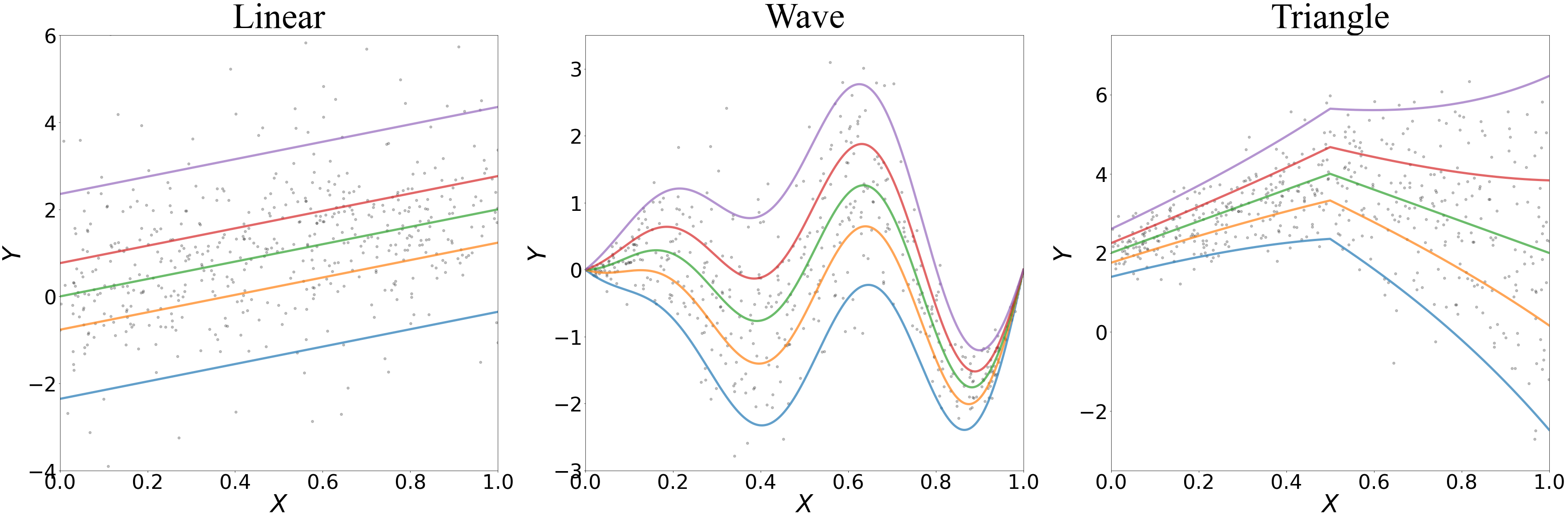
Figure 2: The target quantiles curves. From the left to the right, each column corresponds a data generation model, “Linear”, “Wave” and “Triangle”. The sample data with size $n=512$ is depicted as grey dots.The target quantile functions at the quantile levels $\tau=$0.05 (blue), 0.25 (orange), 0.5 (green), 0.75 (red), 0.95 (purple) are depicted as solid curves.

For these models, we generate $X$ uniformly from the unit interval $[0,1]$. The $\tau$-th conditional quantile of the response $Y$ given $X=x$ can be calculated directly based on the expression of $f_{0}(x,\tau)$. Figure 2 shows all these univariate data generation models and their corresponding conditional quantile curves at $\tau=0.05,0.25,0.50,0.75,0.95$.

Figures 3 to 4 show an instance of the estimated quantile curves for the “Wave” and “Triangle” models. The plot for the “Linear” model is included in the Appendix. In these plots, the training data is depicted as grey dots. The target quantile functions at the quantile levels $\tau=$0.05 (blue), 0.25 (orange), 0.5 (green), 0.75 (red), 0.95 (purple) are depicted as dashed curves, and the estimated quantile functions are represented by solid curves with the same color. For each figure, from the top to the bottom, the rows correspond to the sample size $n=512,2048$. From the left to the right, the columns correspond to the methods DQRP, kernel QR and QR Forest.

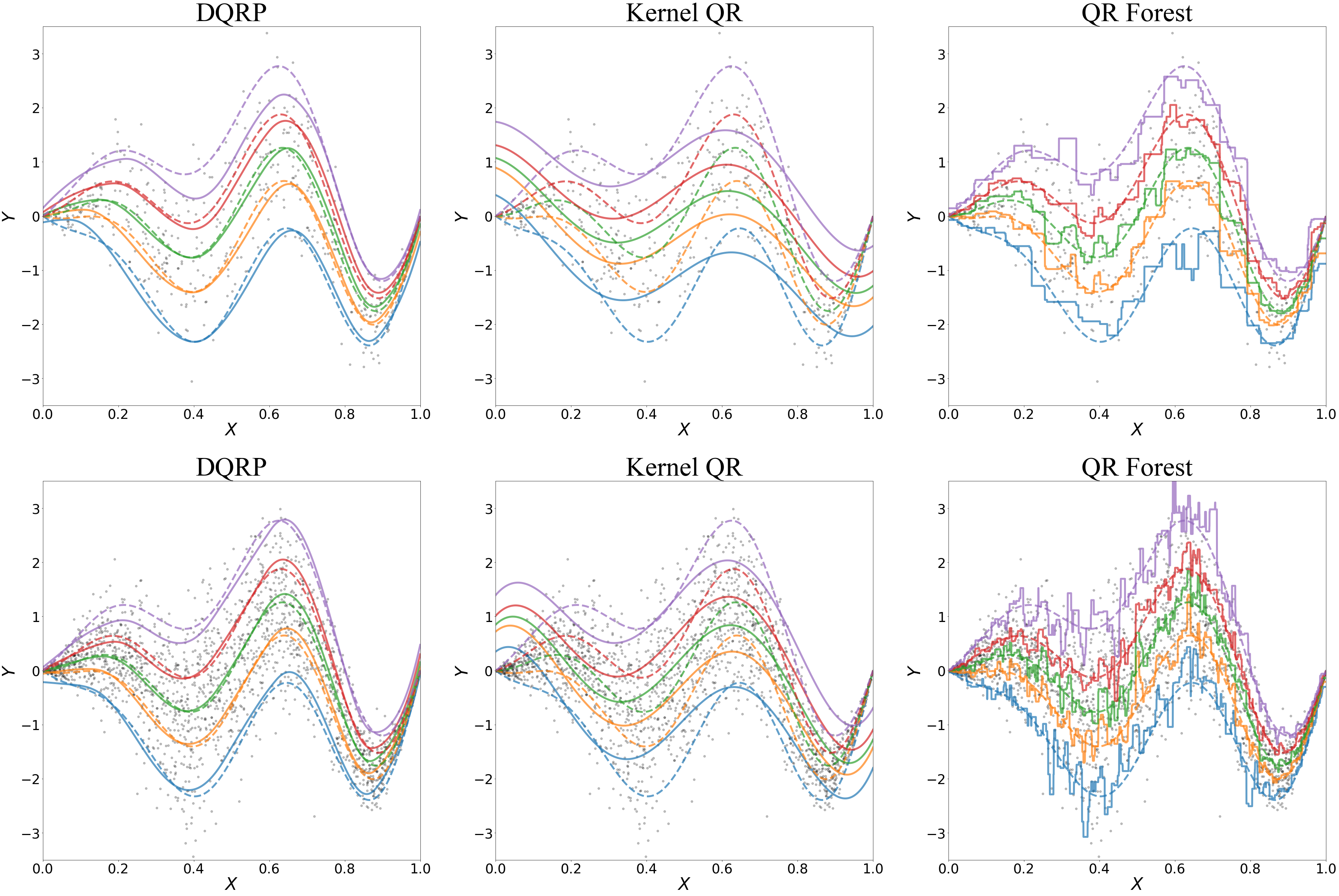
Figure 3: The fitted quantile curves under the univariate “Wave” model. The training data is depicted as grey dots.The target quantile functions at the quantile levels $\tau=$0.05 (blue), 0.25 (orange), 0.5 (green), 0.75 (red), 0.95 (purple) are depicted as dashed curves, and the estimated quantile functions are represented by solid curves with the same color. From the top to the bottom, the rows correspond to the sample size $n=512,2048$. From the left to the right, the columns correspond to the methods DQRP, kernel QR and QR Forest.

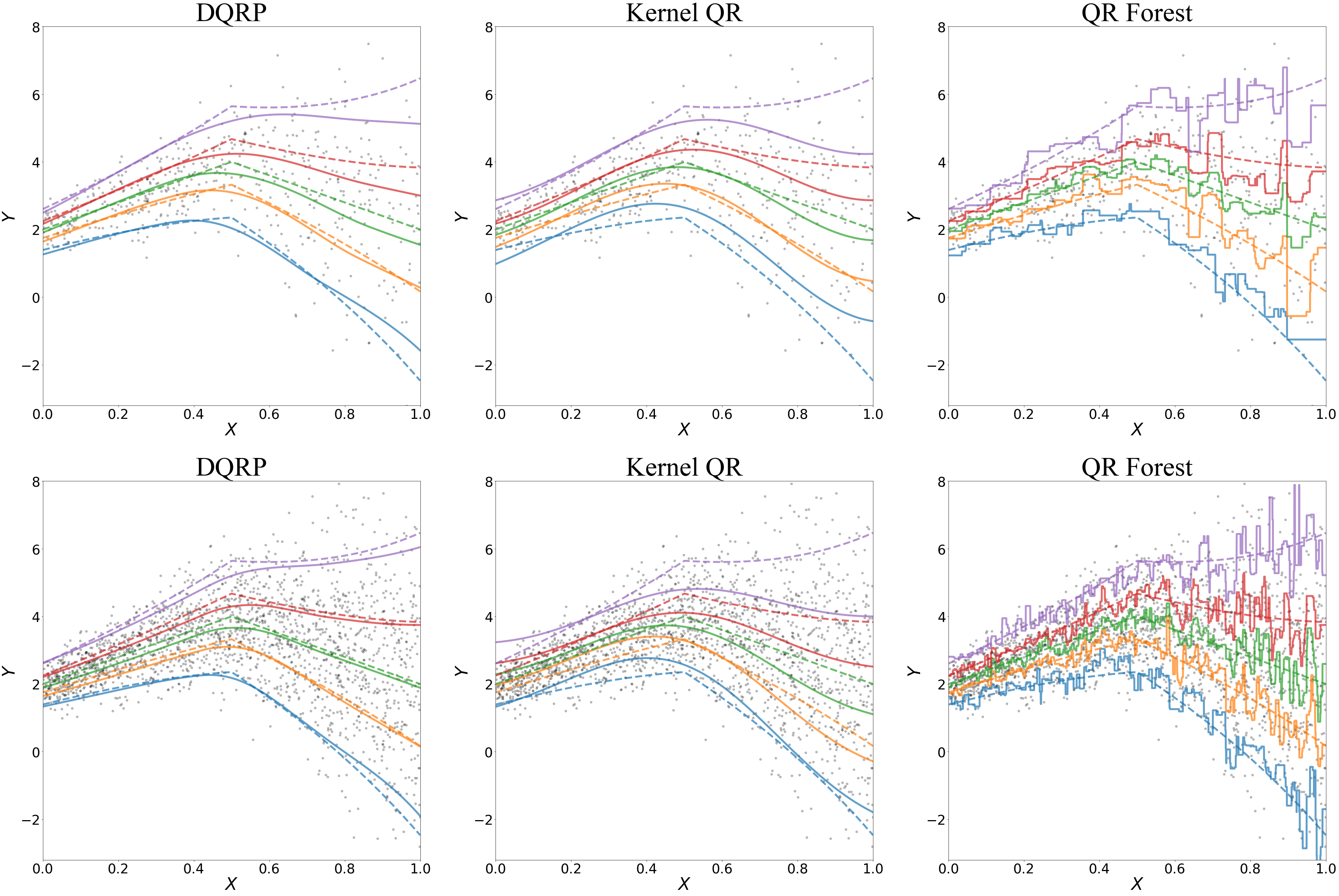
Figure 4: The fitted quantile curves under the univariate “Triangle” model. The training data is depicted as grey dots.The target quantile functions at the quantile levels $\tau=$0.05 (blue), 0.25 (orange), 0.5 (green), 0.75 (red), 0.95 (purple) are depicted as dashed curves, and the estimated quantile functions are represented by solid curves with the same color. From the top to the bottom, the rows correspond to the sample sizes $n=512,2048$. From the left to the right, the columns correspond to the methods DQRP, kernel QR and QR Forest.

Table 1: Data is generated from the “Wave” model with training sample size $n=512,2048$ and the number of replications $R=100$. The averaged $L_{1}$ and $L_{2}^{2}$ test errors with the corresponding standard deviation (in parentheses) are reported for the estimators trained by different methods.

	Sample size	$n=512$		$n=2048$
$\tau$	Method	$L_{1}$	$L_{2}^{2}$	$L_{1}$	$L_{2}^{2}$
0.05	DQRP	0.184(0.072)	0.065(0.061)	0.127(0.055)	0.029(0.026)
	Kernel QR	0.461(0.072)	0.377(0.125)	0.599(0.224)	0.600(0.470)
	QR Forest	0.228(0.030)	0.092(0.024)	0.195(0.017)	0.071(0.013)
0.25	DQRP	0.124(0.041)	0.030(0.023)	0.086(0.034)	0.013(0.011)
	Kernel QR	0.441(0.064)	0.298(0.109)	0.571(0.225)	0.545(0.460)
	QR Forest	0.166(0.024)	0.051(0.015)	0.143(0.012)	0.039(0.007)
0.5	DQRP	0.112(0.030)	0.022(0.012)	0.076(0.024)	0.010(0.006)
	Kernel QR	0.440(0.058)	0.289(0.105)	0.555(0.226)	0.530(0.461)
	QR Forest	0.157(0.024)	0.045(0.014)	0.137(0.010)	0.036(0.005)
0.75	DQRP	0.131(0.047)	0.030(0.023)	0.087(0.030)	0.013(0.009)
	Kernel QR	0.462(0.055)	0.322(0.107)	0.560(0.219)	0.546(0.462)
	QR Forest	0.168(0.022)	0.050(0.014)	0.146(0.013)	0.041(0.008)
0.95	DQRP	0.192(0.072)	0.064(0.049)	0.127(0.042)	0.027(0.018)
	Kernel QR	0.552(0.064)	0.469(0.120)	0.615(0.200)	0.648(0.462)
	QR Forest	0.224(0.030)	0.090(0.026)	0.198(0.018)	0.074(0.014)

Table 2: Data is generated from the “Triangle” model with training sample size $n=512,2048$ and the number of replications $R=100$. The averaged $L_{1}$ and $L_{2}^{2}$ test errors with the corresponding standard deviation (in parentheses) are reported for the estimators trained by different methods.

	Sample size	$n=512$		$n=2048$
$\tau$	Method	$L_{1}$	$L_{2}^{2}$	$L_{1}$	$L_{2}^{2}$
0.05	DQRP	0.263(0.103)	0.152(0.135)	0.174(0.081)	0.069(0.074)
	Kernel QR	0.533(0.147)	0.520(0.268)	0.515(0.200)	0.490(0.459)
	QR Forest	0.364(0.061)	0.282(0.115)	0.359(0.031)	0.264(0.053)
0.25	DQRP	0.181(0.079)	0.058(0.054)	0.112(0.047)	0.023(0.018)
	Kernel QR	0.249(0.084)	0.110(0.084)	0.308(0.138)	0.179(0.217)
	QR Forest	0.272(0.044)	0.155(0.061)	0.259(0.021)	0.140(0.026)
0.5	DQRP	0.187(0.078)	0.061(0.057)	0.118(0.060)	0.025(0.023)
	Kernel QR	0.164(0.063)	0.052(0.044)	0.231(0.134)	0.125(0.158)
	QR Forest	0.251(0.040)	0.131(0.053)	0.252(0.021)	0.133(0.026)
0.75	DQRP	0.238(0.110)	0.097(0.093)	0.150(0.900)	0.041(0.049)
	Kernel QR	0.252(0.087)	0.109(0.081)	0.334(0.123)	0.192(0.166)
	QR Forest	0.261(0.043)	0.142(0.059)	0.266(0.024)	0.149(0.031)
0.95	DQRP	0.343(0.197)	0.216(0.259)	0.224(0.135)	0.097(0.118)
	Kernel QR	0.540(0.123)	0.522(0.242)	0.541(0.175)	0.527(0.363)
	QR Forest	0.359(0.057)	0.256(0.090)	0.357(0.033)	0.259(0.053)

Tables 1 and 2 summarize the results for the models “Wave” and “Triangle”, respectively. For Kernel QR, QR Forest and our proposed DQRP estimator, the corresponding $L_{1}$ and $L_{2}^{2}$ errors (standard deviation in parentheses) between the estimates and the target are reported at different quantile levels $\tau=0.05,0.25,0.50,0.75,0.95$. For each column, using bold text we highlight the best method which produces the smallest risk among these three methods. For the “Wave” model, the proposed DQRP outperforms Kernel QR and QR Forest in all the scenarios. For the nonlinear “Triangle” model, DQRP also tends to perform better than Kernel QR and QR Forest. For the “Linear” model, the results from the three methods are comparable, but Kernel QR tends to have better performance. The results for the “Linear” model are given in Table 5 in the Appendix.

7.3 Multivariate models

We consider three basic multivariate models, including linear model (“Linear”), single index model (“SIM”) and additive model (“Additive”), which correspond to different specifications of the target function $f_{0}$. The formulae are given below.

1. Linear:

   $$f_{0}(x,\tau)=2A^{\top}x+F_{t}^{-1}(\tau),$$

2. Single index model:

   $$f_{0}(x,\tau)=\exp(0.1\times A^{\top}x)+|\sin(\pi B^{\top}x)|\Phi^{-1}(\tau),$$

3. Additive model:

   $$f_{0}(x,\tau)=3x_{1}+4(x_{2}-0.5)^{2}+2\sin(\pi x_{3})-5|x_{4}-0.5|+\exp\{0.1(B^{\top}x-0.5)\}\Phi^{-1}(\tau),$$

where $F_{t}(\cdot)$ denotes the cumulative distribution function of the standard Student’s t random variable, $\Phi(\cdot)$ denotes the cumulative distribution function of the standard normal random variable and the parameters ($d$-dimensional vectors)

$$A= (0.409,0.908,0,0,-2.061,0.254,3.024,1.280)^{\top},$$

$$B= (1.386,-0.902,5.437,0,0,-0.482,4.611,0)^{\top}.$$

Table 3: Data is generated from the “Single index model” with training sample size $n=512,2048$ and the number of replications $R=100$. The averaged $L_{1}$ and $L_{2}^{2}$ test errors with the corresponding standard deviation (in parentheses) are reported for the estimators trained by different methods.

	Sample size	$n=512$		$n=1024$
$\tau$	Method	$L_{1}$	$L_{2}^{2}$	$L_{1}$	$L_{2}^{2}$
0.05	DQRP	0.487(0.034)	0.422(0.065)	0.391(0.017)	0.277(0.034)
	Kernel QR	0.641(0.043)	0.596(0.078)	0.620(0.030)	0.561(0.059)
	QR Forest	0.460(0.012)	0.318(0.031)	0.450(0.004)	0.305(0.013)
0.25	DQRP	0.241(0.027)	0.126(0.034)	0.188(0.013)	0.068(0.010)
	Kernel QR	0.462(0.043)	0.330(0.054)	0.486(0.043)	0.361(0.062)
	QR Forest	0.214(0.010)	0.065(0.006)	0.207(0.005)	0.058(0.003)
0.5	DQRP	0.198(0.026)	0.096(0.029)	0.112(0.016)	0.029(0.008)
	Kernel QR	0.339(0.035)	0.188(0.036)	0.346(0.048)	0.193(0.053)
	QR Forest	0.081(0.010)	0.010(0.003)	0.058(0.005)	0.005(0.001)
0.75	DQRP	0.279(0.025)	0.168(0.036)	0.202(0.016)	0.080(0.013)
	Kernel QR	0.453(0.047)	0.317(0.059)	0.492(0.044)	0.368(0.063)
	QR Forest	0.213(0.011)	0.064(0.007)	0.207(0.005)	0.058(0.003)
0.95	DQRP	0.488(0.033)	0.443(0.057)	0.416(0.025)	0.303(0.035)
	Kernel QR	0.637(0.044)	0.589(0.080)	0.627(0.033)	0.572(0.066)
	QR Forest	0.459(0.010)	0.317(0.028)	0.451(0.005)	0.306(0.014)

Table 4: Data is generated from the “Additive” model with training sample size $n=512,2048$ and the number of replications $R=100$. The averaged $L_{1}$ and $L_{2}^{2}$ test errors with the corresponding standard deviation (in parentheses) are reported for the estimators trained by different methods.

	Sample size	$n=512$		$n=1024$
$\tau$	Method	$L_{1}$	$L_{2}^{2}$	$L_{1}$	$L_{2}^{2}$
0.05	DQRP	0.263(0.103)	0.152(0.135)	0.174(0.081)	0.069(0.074)
	Kernel QR	0.533(0.147)	0.520(0.268)	0.515(0.200)	0.490(0.459)
	QR Forest	0.364(0.061)	0.282(0.115)	0.359(0.031)	0.264(0.053)
0.25	DQRP	0.181(0.079)	0.058(0.054)	0.112(0.047)	0.023(0.018)
	Kernel QR	0.249(0.084)	0.110(0.084)	0.308(0.138)	0.179(0.217)
	QR Forest	0.272(0.044)	0.155(0.061)	0.259(0.021)	0.140(0.026)
0.5	DQRP	0.187(0.078)	0.061(0.057)	0.118(0.060)	0.025(0.023)
	Kernel QR	0.164(0.063)	0.052(0.044)	0.231(0.134)	0.125(0.158)
	QR Forest	0.251(0.040)	0.131(0.053)	0.252(0.021)	0.133(0.026)
0.75	DQRP	0.238(0.110)	0.097(0.093)	0.150(0.900)	0.041(0.049)
	Kernel QR	0.252(0.087)	0.109(0.081)	0.334(0.123)	0.192(0.166)
	QR Forest	0.261(0.043)	0.142(0.059)	0.266(0.024)	0.149(0.031)
0.95	DQRP	0.343(0.197)	0.216(0.259)	0.224(0.135)	0.097(0.118)
	Kernel QR	0.540(0.123)	0.522(0.242)	0.541(0.175)	0.527(0.363)
	QR Forest	0.359(0.057)	0.256(0.090)	0.357(0.033)	0.259(0.053)

The simulation results under multivariate “SIM” and “Additive” models are summarized in Tables 3-4 respectively. For Kernel QR, QR Forest and our proposed DQRP, the corresponding $L_{1}$ and $L_{2}^{2}$ distances (standard deviation in parentheses) between the estimates and the target are reported at different quantile levels $\tau=0.05,0.25,0.50,0.75,0.95$. For each column, using bold text we highlight the best method which produces the smallest risk among these three methods.

7.4 Tuning Parameter

In this subsection, we study the effects of the tuning parameter $\lambda$ on the proposed method. First, we demonstrate that the “quantile crossing” phenomenon can be mitigated. We apply our method to the bone mineral density (BMD) dataset. This dataset is originally reported in Bachrach et al. (1999) and analyzed in Takeuchi et al. (2006); Hastie et al. (2009). The dataset collects the bone mineral density data of 485 North American adolescents ranging from 9.4 years old to 25.55 years old. Each response value is the difference of the bone mineral density taken on two consecutive visits, divided by the average. The predictor age is the averaged age over the two visits.

In Figure 5, we present the estimated quantile regression processes with ($\lambda=\log(n)$) or without ($\lambda=0$) the proposed non-crossing penalty. With or without the penalty, we use the Adam optimizer with the same parameters (for the optimization process) to train a fixed-shape ReQU network with three hidden layers and width $(128,128,128)$. The estimated quantile curves at $\tau=0.1,0.2,\ldots,0.9$ and the observations are depicted in Figure 5. It can be seen that the proposed non-crossing penalty is effective to avoid quantile crossing, even in the area outside the range of the training data.

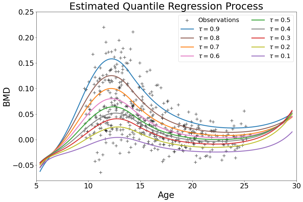
(a) Without non-crossing penalty

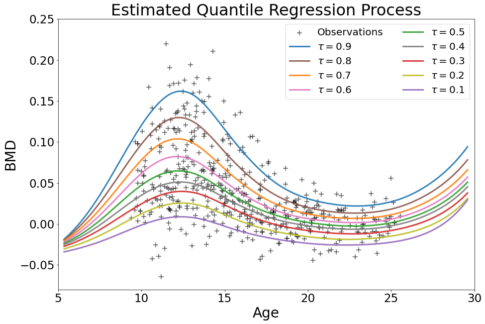
(b) With non-crossing penalty

Figure 5: An example of quantile crossing problem in BMD data set. The estimated quantile curves at $\tau=0.1,0.2,\ldots,0.9$ and the observations are depicted. In the left panel, the estimation is conducted without non-crossing penalty and there are crossings at both edges of the graph. In the right figure, the estimation is conducted with non-crossing penalty. There is no quantile crossing even in the area outside the range of the training data.

Second, we study how the value of tuning parameter $\lambda$ affects the risk of the estimated quantile regression process and how it helps avoiding crossing. Given a sample with size $n$, we train a series of the DQRP estimators at different values of the tuning parameter $\lambda$. For each DQRP estimator, we record its risk and penalty values and the track of these values are plotted in Figures 6-7. For each obtained DQRP estimator $\hat{f}^{\lambda}_{n}$, the statistics “Risk” is calculated according to the formula

$$\mathcal{R}(\hat{f}^{\lambda}_{n})=\mathbb{E}_{X,Y,\xi}\{\rho_{\xi}(Y-f(X,\xi))\},$$

and the statistics “Penalty” is calculated according to

$$\kappa(\hat{f}^{\lambda}_{n})=\mathbb{E}_{X,\xi}[\max\{-\frac{\partial}{\partial\tau}\hat{f}^{\lambda}_{n}(X,\xi),0\}].$$

In practice, we generate $T=10,000$ testing data $(X_{t}^{test},Y_{t}^{test},\xi_{t}^{tesr})_{t=1}^{T}$ to empirically calculate risks and penalty values.

In each figure, a vertical dashed line is also depicted at the value $\lambda=\log(n)$. It can be seen that crossing seldom happens when we choose a tiny value of the tuning parameter $\lambda$. And the loss caused by penalty can be negligible compared to the total risk, since the penalty values are generally of order $O(10^{-3})$ instead of $O(10^{3})$ for the total risk. For large value of tuning parameter $\lambda$, the crossing nearly disappears which is intuitive and encouraged by the formulation of our penalty. However, the risk could be very large resulting a poor estimation of the target function. As shown by the dashed vertical line in each figure, numerically the choice of $\lambda=\log(n)$ can lead to a reasonable estimation of the target function with tiny risk (blue lines) and little crossing (red lines) across different model settings. Empirically, we choose $\lambda=\log(n)$ in general for the simulations. By Theorem 1, such choice of tuning parameter can lead to a consistent estimator with reasonable fast rate of convergence.

Figure 6: The value of risks and penalties under the univariate “Triangle” model when $n=512,2048$. A vertical dashed line is depicted at the value $\lambda=\log(n)$ on x-axis in each figure.

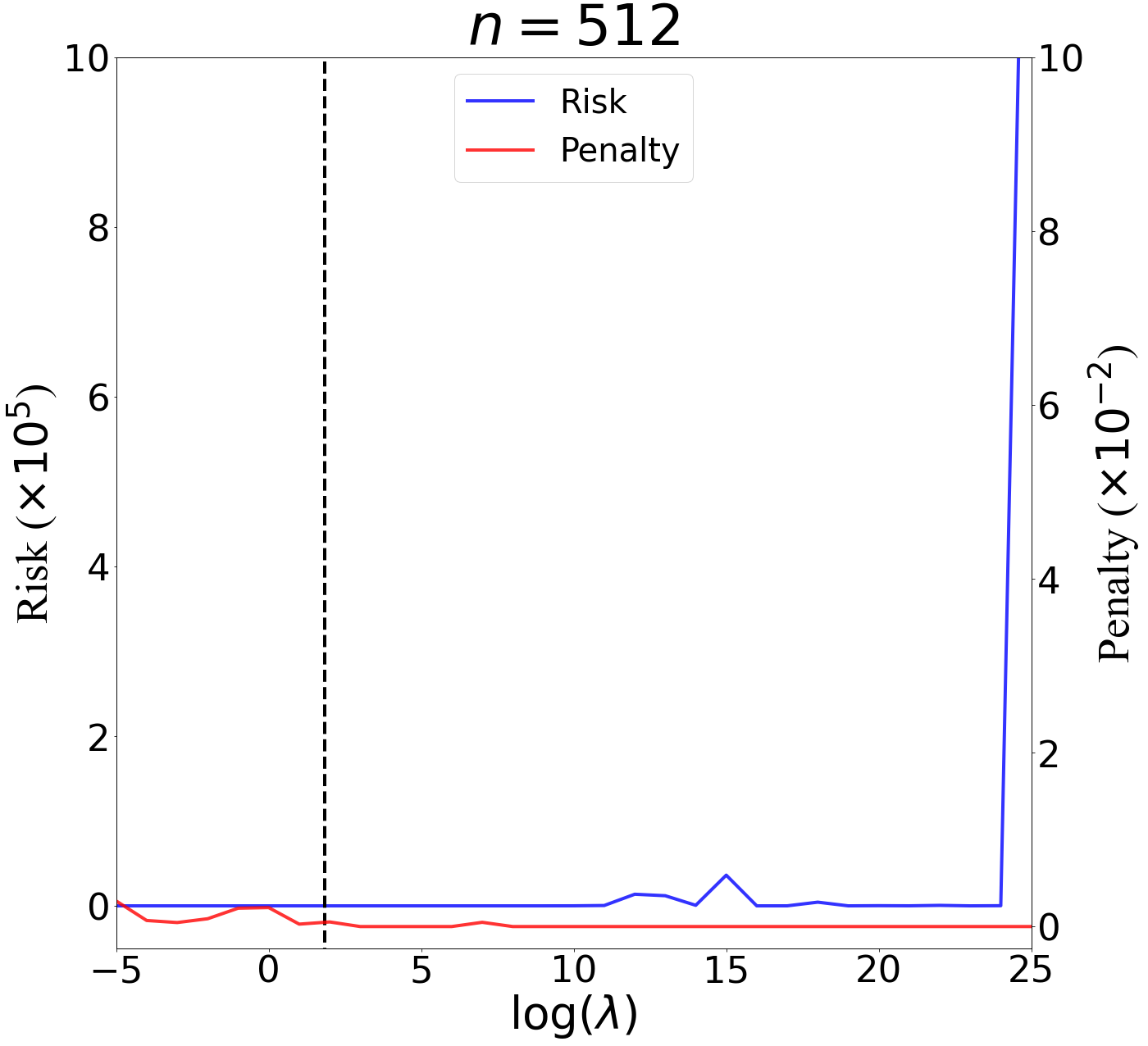
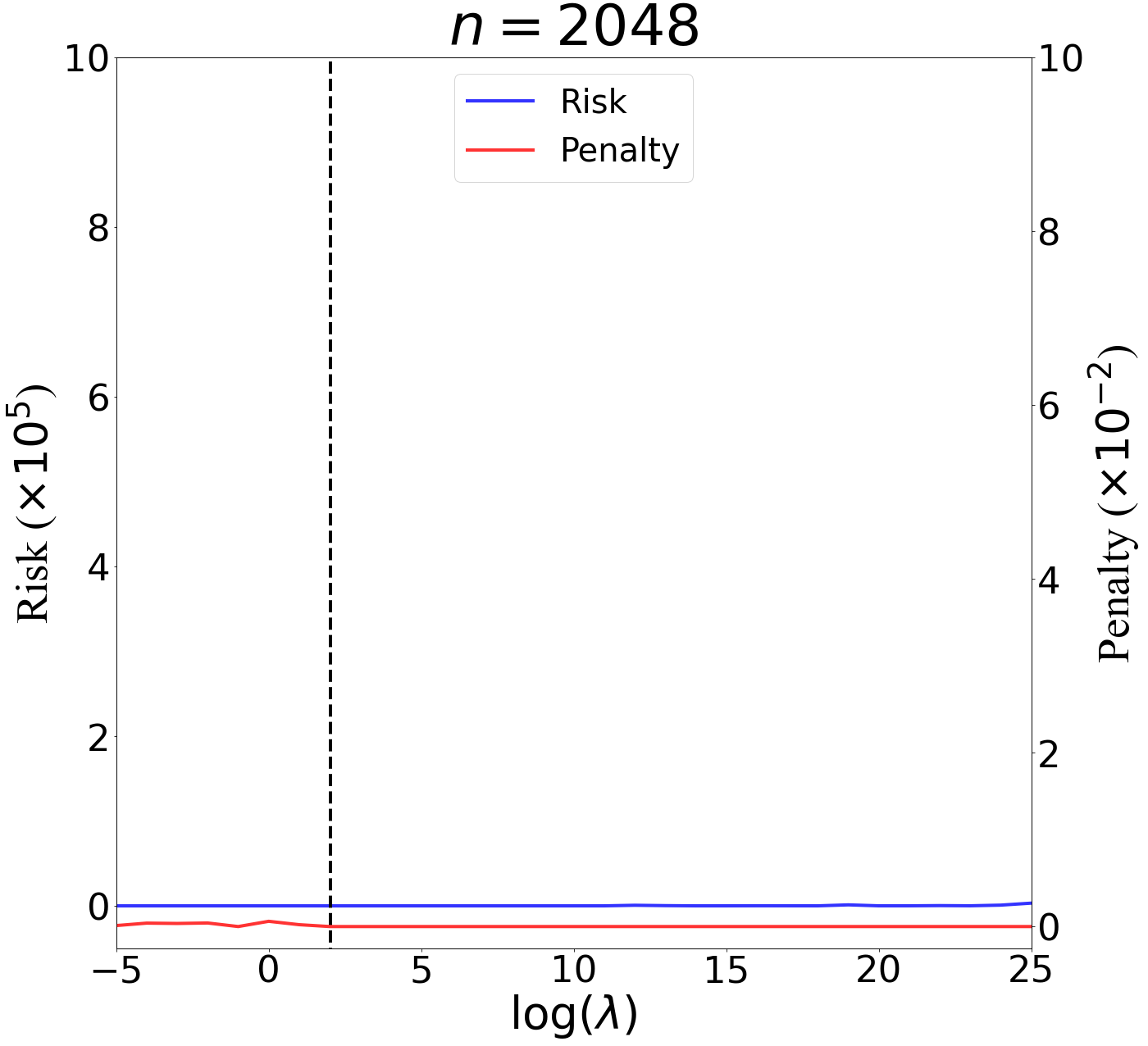
Figure 7: The value of risks and penalties under the multivariate additive model when $n=512,2048$ and $d=8$. A vertical dashed line is depicted at the value $\lambda=\log(n)$ on x-axis in each figure.

8 Conclusion

We have proposed a penalized nonparametric approach to estimating the nonseparable model (1.1) using ReQU activated deep neural networks and introduced a novel penalty function to enforcing non-crossing quantile curves. We have established non-asymptotic excess risk bounds for the estimated QRP and derived the mean integrated squared error for the estimated QRP under mild smoothness and regularity conditions. We have also developed a new approximation error bound for $C^{s}$ smooth functions with smoothness index $s>0$ using ReQU activated neural networks. Our numerical experiments demonstrate that the proposed method is competitive with or outperforms two existing methods, including methods using reproducing kernels and random forests, for nonparmetric quantile regression. Therefore, the proposed approach can be a useful addition to the methods for multivariate nonparametric regression analysis.

The results and methods of this work are expected to be useful in other settings. In particular, our approximation results on ReQU activated networks are of independent interest. It would be interesting to take advantage of the smoothness of ReQU activated networks and use them in other nonparametric estimation problems, such as the estimation of a regression function and its derivative.

Appendix A Proof of Theorems, Corollaries and Lemmas

In the appendix, we include the proofs for the results stated in Section 3 and the technical details needed in the proofs.

Proof of Proposition 1

For any random variable $\xi$ supported on $(0,1)$, the risk

$$\mathcal{R}(f)= \mathbb{E}_{X,Y,\xi}\{\rho_{\xi}(Y-f(X,\xi))\}$$

$$= \int_{0}^{1}\mathbb{E}_{X,Y}\{\rho_{\xi}(Y-f(X,\tau))\}\pi_{\xi}(\tau)d\tau$$

where $\pi_{\xi}(\cdot)\geq 0$ is the density function of $\xi$. By the definition of $f_{0}$ and the property of quantile loss function, it is known $f_{0}$ minimizes $\mathbb{E}_{X,Y}\{\rho_{\xi}(Y-f(X,\tau))\}$ as well as $\mathbb{E}_{X,Y}\{\rho_{\xi}(Y-f(X,\tau))\}\pi_{\xi}(\tau)$ for each $\tau\in(0,1)$. Thus $f_{0}$ minimizes the integral or the risk $\mathcal{R}(\cdot)$ over measurable functions.

Note that if $\pi_{\xi}(\tau)=0$ for some $\tau\in T$ where $T$ is a subset of $(0,1)$, then any function $\tilde{f}_{0}$ defined on $\mathcal{X}\times(0,1)$ that is different from $f_{0}$ only on $\mathcal{X}\times T$ will also be a minimizer of $\mathcal{R}(\cdot)$. To be exact,

$$\tilde{f}_{0}\in\arg\min_{f}\mathcal{R}(f)\qquad{\rm if\ and\ only\ if}\qquad\tilde{f}_{0}=f_{0}{\rm\ on\ }\mathcal{X}\times T.$$

Further, if $(X,\xi)$ has non zero density almost everywhere on $\mathcal{X}\times(0,1)$ and the probability measure of $(X,\xi)$ is absolutely continuous with respect to Lebesgue measure, then above defined set $\mathcal{X}\times T$ is measure-zero and $f_{0}$ is the unique minimizer of $\mathcal{R}(\cdot)$ over all measurable functions in the sense of almost everywhere(almost surely), i.e.,

$$f_{0}=\arg\min_{f}\mathcal{R}(f)=\arg\min_{f}\mathbb{E}_{X,Y,\xi}\{\rho_{\xi}(Y-f(X,\xi))\},$$

up to a negligible set with respect to the probability measure of $(X,\eta)$ on $\mathcal{X}\times(0,1)$. $\hfill\Box$

Proof of Lemma 1

Recall that $\hat{f}^{\lambda}_{n}$ is the penalized empirical risk minimizer. Then, for any $f\in\mathcal{F}_{n}$ we have

$$\mathcal{R}^{\lambda}_{n}(\hat{f}^{\lambda}_{n})\leq\mathcal{R}^{\lambda}_{n}(f).$$

Besides, for any $f\in\mathcal{F}$ we have $\kappa(f)\geq 0$ and $\kappa_{n}(f)\geq 0$ since $\kappa$ and $\kappa_{n}$ are nonnegative functions. Note that $\kappa(f_{0})=\kappa_{n}(f_{0})=0$ by the assumption that $f_{0}$ is increasing in its second argument. Then,

$$\mathcal{R}(\hat{f}^{\lambda}_{n})-\mathcal{R}(f_{0})\leq \mathcal{R}(\hat{f}^{\lambda}_{n})-\mathcal{R}(f_{0})+\lambda\{\kappa(\hat{f}^{\lambda}_{n})-\kappa(f_{0})\}=\mathcal{R}^{\lambda}(\hat{f}^{\lambda}_{n})-\mathcal{R}^{\lambda}(f_{0}).$$

We can then give upper bounds for the excess risk $\mathcal{R}(\hat{f}^{\lambda}_{n})-\mathcal{R}(f_{0})$. For any $f\in\mathcal{F}_{n}$,

$$\mathbb{E}\{\mathcal{R}(\hat{f}^{\lambda}_{n})-\mathcal{R}(f_{0})\}$$

$$\leq\mathbb{E}\{\mathcal{R}^{\lambda}(\hat{f}^{\lambda}_{n})-\mathcal{R}^{\lambda}(f_{0})\}$$

$$\leq\mathbb{E}\{\mathcal{R}^{\lambda}(\hat{f}^{\lambda}_{n})-\mathcal{R}^{\lambda}(f_{0})\}+2\mathbb{E}\{\mathcal{R}_{n}^{\lambda}(f)-\mathcal{R}_{n}^{\lambda}(\hat{f}^{\lambda}_{n})\}$$

$$=\mathbb{E}\{\mathcal{R}^{\lambda}(\hat{f}^{\lambda}_{n})-\mathcal{R}^{\lambda}(f_{0})\}+2\mathbb{E}[\{\mathcal{R}_{n}^{\lambda}(f)-\mathcal{R}_{n}^{\lambda}(f_{0})\}-\{\mathcal{R}_{n}^{\lambda}(\hat{f}^{\lambda}_{n})-\mathcal{R}_{n}^{\lambda}(f_{0})\}]$$

$$=\mathbb{E}\{\mathcal{R}^{\lambda}(\hat{f}^{\lambda}_{n})-2\mathcal{R}^{\lambda}_{n}(\hat{f}^{\lambda}_{n})+\mathcal{R}^{\lambda}(f_{0})\}+2\mathbb{E}\{\mathcal{R}_{n}^{\lambda}(f)-\mathcal{R}_{n}^{\lambda}(f_{0})\}$$

where the second inequality holds by the the fact that $\hat{f}^{\lambda}_{n}$ satisfies $\mathcal{R}_{n}^{\lambda}(f)\geq\mathcal{R}_{n}^{\lambda}(\hat{f}^{\lambda}_{n})$ for any $f\in\mathcal{F}_{n}$. Since the inequality holds for any $f\in\mathcal{F}_{n}$, we have

$$\mathbb{E}\{\mathcal{R}(\hat{f}^{\lambda}_{n})-\mathcal{R}(f_{0})\} \leq\mathbb{E}\{\mathcal{R}^{\lambda}(\hat{f}^{\lambda}_{n})-2\mathcal{R}^{\lambda}_{n}(\hat{f}^{\lambda}_{n})+\mathcal{R}^{\lambda}(f_{0})\}+2\inf_{f\in\mathcal{F}_{n}}\{\mathcal{R}^{\lambda}(f)-\mathcal{R}^{\lambda}(f_{0})\}.$$

This completes the proof. $\hfill\Box$

Proof of Theorem 1

The proof is straightforward by consequences of Theorem 3 and Corollary 1.

For any $N\in\mathbb{N}^{+}$, let $\mathcal{F}_{n}:=\mathcal{F}_{\mathcal{D},\mathcal{W},\mathcal{U},\mathcal{S},\mathcal{B},\mathcal{B}^{\prime}}$ be the ReQU activated neural networks $f:\mathcal{X}\times(0,1)\to\mathbb{R}$ with depth $\mathcal{D}\leq 2N-1$, width $\mathcal{W}\leq 12N^{d}$, number of neurons $\mathcal{U}\leq 15N^{d+1}$, number of parameters $\mathcal{S}\leq 24N^{d+1}$ and satisfying $\mathcal{B}\geq\|f_{0}\|_{C^{0}}$ and $\mathcal{B}^{\prime}\geq\|f_{0}\|_{C^{1}}$. Then we would compare the stochastic error bounds $8602{\mathcal{U}\mathcal{S}}$ and $5796{\mathcal{D}\mathcal{S}(\mathcal{D}+\log_{2}U)}$. By simple math it can be shown that ${\mathcal{D}\mathcal{S}}(\mathcal{D}+\log_{2}U)=\mathcal{O}(dN^{d+3})$ and $\mathcal{U}\mathcal{S}=\mathcal{O}(N^{2d+2})$. Since $d\geq 1$, then we choose apply the upper bound $\mathcal{D}\mathcal{S}(\mathcal{D}+\log_{2}U)$ in Theorem 3 to get a excess risk bound with lower order in terms of $N$. This completes the proof. $\hfill\Box$

Proof of Lemma 3

Let $\sigma_{1}(x)=\max\{0,x\}$ and $\sigma_{2}(x)=\max\{0,x\}^{2}$ denote the ReLU and ReQU activation functions respectively. Let $(d_{0},d_{1},\ldots,d_{\mathcal{D}+1})$ be vector of the width (number of neurons) of each layer in the original ReQU network where $d_{0}=d+1$ and $d_{\mathcal{D}+1}=1$ in our problem. We let $f^{(i)}_{j}$ be the function (subnetwork of the ReQU network) from $\mathcal{X}\times(0,1)\subset\mathbb{R}^{d+1}$ to $\mathbb{R}$ which takes $(X,\xi)=(x_{1},\ldots,x_{d},x_{d+1})$ as input and outputs the $j$-th neuron of the $i$-th layer for $j=1,\ldots,d_{i}$ and $i=1,\ldots,\mathcal{D}+1$.

We next construct iteratively ReLU-ReQU activated subnetworks to compute $(\frac{\partial}{\partial\tau}f^{(i)}_{1},\ldots,f^{(i)}_{d_{i}})$ for $i=1,\ldots,\mathcal{D}+1$, i.e., the partial derivatives of the original ReQU subnetworks step by step. We illustrate the details of the construction of the ReLU-ReQU subnetworks for the first two layers ($i=1,2$) and the last layer $(\i=\mathcal{D}+1)$ and apply induction for layers $i=3,\ldots,\mathcal{D}$. Note that the derivative of ReQU activation function is $\sigma^{\prime}_{2}(x)=2\sigma_{1}(x)$, then when $i=1$ for any $j=1,\ldots,d_{1}$,

$$\frac{\partial}{\partial\tau}f^{(1)}_{j}=\frac{\partial}{\partial\tau}\sigma_{2}\Big{(}\sum_{i=1}^{d+1}w^{(1)}_{ji}x_{i}+b_{j}^{(1)}\Big{)}=2\sigma_{1}\Big{(}\sum_{i=1}^{d+1}w^{(1)}_{ji}x_{i}+b_{j}^{(1)}\Big{)}\cdot w_{j,d+1}^{(1)},$$ (A.1)

where we denote $w^{(1)}_{ji}$ and $b_{j}^{(1)}$ by the corresponding weights and bias in $1$-th layer of the original ReQU network and with a little bit abuse of notation we view $x_{d+1}$ as the argument $\tau$ and calculate its partial derivative. Now we intend to construct a 4 layer (2 hidden layers) ReLU-ReQU network with width $(d_{0},3d_{1},10d_{1},2d_{1})$ which takes $(X,\xi)=(x_{1},\ldots,x_{d},x_{d+1})$ as input and outputs

$$(f^{(1)}_{1},\ldots,f^{(1)}_{d_{1}},\frac{\partial}{\partial\tau}f^{(1)}_{1},\ldots,\frac{\partial}{\partial\tau}f^{(1)}_{d_{1}})\in\mathbb{R}^{2d_{1}}.$$

Note that the output of such network contains all the quantities needed to calculated $(\frac{\partial}{\partial\tau}f^{(2)}_{1},\ldots,\frac{\partial}{\partial\tau}f^{(2)}_{d_{2}})$, and the process of construction can be continued iteratively and the induction proceeds. In the firstly hidden layer, we can obtain $3d_{1}$ neurons

$$(f^{(1)}_{1},\ldots,f^{(1)}_{d_{1}},|w^{(1)}_{1,d_{0}}|,\ldots,|w^{(1)}_{d_{1},d_{0}}|,\sigma_{1}(\sum_{i=1}^{d_{0}}w^{(1)}_{1i}x_{i}+b^{(1)}_{1}),\ldots,\sigma_{1}(\sum_{i=1}^{d_{0}}w^{(1)}_{d_{1}i}x_{i}+b^{(1)}_{d_{1}})),$$

with weight matrix $A^{(1)}_{1}$ having $2d_{0}d_{1}$ parameters, bias vector $B^{(1)}_{1}$ and activation function vector $\Sigma_{1}$ being

$$A^{(1)}_{1}=\left[\begin{array}[]{ccccc}w^{(1)}_{1,1}&w^{(1)}_{1,2}&\cdots&\cdots&w^{(1)}_{1,d_{0}}\\ w^{(1)}_{2,1}&w^{(1)}_{2,2}&\cdots&\cdots&w^{(1)}_{2,d_{0}}\\ \ldots&\ldots&\ldots&\ldots&\ldots\\ w^{(1)}_{d_{1},1}&w^{(1)}_{d_{1},2}&\cdots&\cdots&w^{(1)}_{d_{1},d_{0}}\\ 0&0&0&0&0\\ \ldots&\ldots&\ldots&\ldots&\ldots\\ 0&0&0&0&0\\ w^{(1)}_{1,1}&w^{(1)}_{1,2}&\cdots&\cdots&w^{(1)}_{1,d_{0}}\\ w^{(1)}_{2,1}&w^{(1)}_{2,2}&\cdots&\cdots&w^{(1)}_{2,d_{0}}\\ \ldots&\ldots&\ldots&\ldots&\ldots\\ w^{(1)}_{d_{1},1}&w^{(1)}_{d_{1},2}&\cdots&\cdots&w^{(1)}_{d_{1},d_{0}}\\ \end{array}\right]\in\mathbb{R}^{3d_{1}\times d_{0}},\quad B^{(1)}_{1}=\left[\begin{array}[]{c}b^{(1)}_{1}\\ b^{(1)}_{2}\\ \ldots\\ b^{(1)}_{d_{1}}\\ |w^{(1)}_{1,d_{0}}|\\ |w^{(1)}_{2,d_{0}}|\\ \ldots\\ |w^{(1)}_{d_{1},d_{0}}|\\ b^{(1)}_{1}\\ b^{(1)}_{2}\\ \ldots\\ b^{(1)}_{d_{1}}\\ \end{array}\right]\in\mathbb{R}^{3d_{1}},\quad\Sigma^{(1)}_{1}=\left[\begin{array}[]{c}\sigma_{2}\\ \ldots\\ \sigma_{2}\\ \sigma_{1}\\ \ldots\\ \sigma_{1}\\ \sigma_{1}\\ \ldots\\ \sigma_{1}\\ \end{array}\right],$$

where the first $d_{1}$ activation functions of $\Sigma_{1}$ are chosen to be $\sigma_{2}$ and others $\sigma_{1}$. In the second hidden layer, we can obtain $10d_{1}$ neurons. The first $2d_{1}$ neurons of the second hidden layer (or the third layer) are

$$(\sigma_{1}(f^{(1)}_{1}),\sigma_{1}(-f^{(1)}_{1})),\ldots,\sigma_{1}(f^{(1)}_{d_{1}}),\sigma_{1}(f^{(1)}_{d_{1}})),$$

which intends to implement identity map such that $(f^{(1)}_{1},\ldots,f^{(1)}_{d_{1}})$ can be kept and outputted in the next layer since identity map can be realized by $x=\sigma_{1}(x)-\sigma_{1}(-x)$. The first $8d_{1}$ neurons of the second hidden layer (or the third layer) are

$$\left[\begin{array}[]{c}\sigma_{2}(w^{(1)}_{1,d_{0}}+\sigma_{1}(\sum_{i=1}^{d_{0}}w^{(1)}_{1i}x_{i}+b^{(1)}_{1}))\\ \sigma_{2}(w^{(1)}_{1,d_{0}}-\sigma_{1}(\sum_{i=1}^{d_{0}}w^{(1)}_{1i}x_{i}+b^{(1)}_{1}))\\ \sigma_{2}(-w^{(1)}_{1,d_{0}}+\sigma_{1}(\sum_{i=1}^{d_{0}}w^{(1)}_{1i}x_{i}+b^{(1)}_{1})\\ \sigma_{2}(-w^{(1)}_{1,d_{0}}-\sigma_{1}(\sum_{i=1}^{d_{0}}w^{(1)}_{1i}x_{i}+b^{(1)}_{1}))\\ \ldots\\ \sigma_{2}(w^{(1)}_{d_{1},d_{0}}+\sigma_{1}(\sum_{i=1}^{d_{0}}w^{(1)}_{d_{1}i}x_{i}+b^{(1)}_{d_{1}}))\\ \sigma_{2}(w^{(1)}_{d_{1},d_{0}}-\sigma_{1}(\sum_{i=1}^{d_{0}}w^{(1)}_{d_{1}i}x_{i}+b^{(1)}_{d_{1}}))\\ \sigma_{2}(-w^{(1)}_{d_{1},d_{0}}+\sigma_{1}(\sum_{i=1}^{d_{0}}w^{(1)}_{d_{1}i}x_{i}+b^{(1)}_{d_{1}})\\ \sigma_{2}(-w^{(1)}_{d_{1},d_{0}}-\sigma_{1}(\sum_{i=1}^{d_{0}}w^{(1)}_{d_{1}i}x_{i}+b^{(1)}_{d_{1}}))\\ \end{array}\right]\in\mathbb{R}^{8d_{1}},$$

which is ready for implementing the multiplications in (A.1) to obtain $(\frac{\partial}{\partial\tau}f^{(1)}_{1},\ldots,\frac{\partial}{\partial\tau}f^{(1)}_{d_{1}})\in\mathbb{R}^{d_{1}}$ since

$$x\cdot y=\frac{1}{4}\{(x+y)^{2}-(x-y)^{2}\}=\frac{1}{4}\{\sigma_{2}(x+y)+\sigma_{2}(-x-y)-\sigma_{2}(x-y)-\sigma_{2}(-x+y)\}.$$

In the second hidden layer (the third layer), the bias vector is zero $B^{(1)}_{2}=(0,\ldots,0)\in\mathbb{R}^{10d_{1}}$, activation functions vector

$$\Sigma^{(1)}_{2}=(\underbrace{\sigma_{1},\ldots,\sigma_{1}}_{2d_{1}\ {\rm times}},\underbrace{\sigma_{2},\ldots,\sigma_{2}}_{8d_{1}\ {\rm times}}),$$

and the corresponding weight matrix $A^{(1)}_{2}$ can be formulated correspondingly without difficulty which contains $2d_{1}+8d_{1}=10d_{1}$ non-zero parameters. Then in the last layer, by the identity maps and multiplication operations with weight matrix $A^{(1)}_{3}$ having $2d_{1}+4d_{1}=6d_{1}$ parameters, bias vector $B^{(1)}_{3}$ being zeros, we obtain

$$(f^{(1)}_{1},\ldots,f^{(1)}_{d_{1}},\frac{\partial}{\partial\tau}f^{(1)}_{1},\ldots,\frac{\partial}{\partial\tau}f^{(1)}_{d_{1}})\in\mathbb{R}^{2d_{1}}.$$

Such ReLU-ReQU neural network has 2 hidden layers (4 layers), $15d_{1}$ hidden neurons, $2d_{0}d_{1}+3d_{1}+10d_{1}+6d_{1}=2d_{0}d_{1}+19d_{1}$ parameters and its width is $(d_{0},3d_{1},10d_{1},2d_{1})$. It worth noting that the ReLU-ReQU activation functions do not apply to the last layer since the construction here is for a single network. When we are combining two consecutive subnetworks into one long neural network, the ReLU-ReQU activation functions should apply to the last layer of the first subnetwork. Hence, in the construction of the whole big network, the last layer of the subnetwork here should output $4d_{1}$ neurons

$$(\sigma_{1}(f^{(1)}_{1}),\sigma_{1}(-f^{(1)}_{1})\ldots,\sigma_{1}(f^{(1)}_{d_{1}}),\sigma_{1}(-f^{(1)}_{d_{1}}),$$

$$\qquad\sigma_{1}(\frac{\partial}{\partial\tau}f^{(1)}_{1}),\sigma_{1}(-\frac{\partial}{\partial\tau}f^{(1)}_{1})\ldots,\sigma_{1}(\frac{\partial}{\partial\tau}f^{(1)}_{d_{1}}),\sigma_{1}(-\frac{\partial}{\partial\tau}f^{(1)}_{d_{1}}))\in\mathbb{R}^{4d_{1}},$$

to keep $(f^{(1)}_{1},\ldots,f^{(1)}_{d_{1}},\frac{\partial}{\partial\tau}f^{(1)}_{1},\ldots,\frac{\partial}{\partial\tau}f^{(1)}_{d_{1}})$ in use in the next subnetwork. Then for this ReLU-ReQU neural network, the weight matrix $A^{(1)}_{3}$ has $2d_{1}+8d_{1}=10d_{1}$ parameters, the bias vector $B^{(1)}_{3}$ is zeros and the activation functions vector $\Sigma^{(1)}_{3}$ has all $\sigma_{1}$ as elements. And such ReLU-ReQU neural network has 2 hidden layers (4 layers), $17d_{1}$ hidden neurons, $2d_{0}d_{1}+3d_{1}+10d_{1}+10d_{1}=2d_{0}d_{1}+23d_{1}$ parameters and its width is $(d_{0},3d_{1},10d_{1},4d_{1})$.

Now we consider the second step, for any $j=1,\ldots,d_{2}$,

$$\frac{\partial}{\partial\tau}f^{(2)}_{j}=\frac{\partial}{\partial\tau}\sigma_{2}\Big{(}\sum_{i=1}^{d_{1}}w^{(2)}_{ji}f^{(1)}_{i}+b_{j}^{(2)}\Big{)}=2\sigma_{1}\Big{(}\sum_{i=1}^{d_{1}}w^{(2)}_{ji}f^{(1)}_{i}+b_{j}^{(2)}\Big{)}\cdot\sum_{i=1}^{d_{1}}w_{j,i}^{(2)}\frac{\partial}{\partial\tau}f^{(1)}_{i},$$ (A.2)

where $w^{(2)}_{ji}$ and $b_{j}^{2)}$ are defined correspondingly as the weights and bias in $2$-th layer of the original ReQU network. By the previous constructed subnetwork, we can start with its outputs

$$(\sigma_{1}(f^{(1)}_{1}),\sigma_{1}(-f^{(1)}_{1})\ldots,\sigma_{1}(f^{(1)}_{d_{1}}),\sigma_{1}(-f^{(1)}_{d_{1}}),$$

$$\qquad\sigma_{1}(\frac{\partial}{\partial\tau}f^{(1)}_{1}),\sigma_{1}(-\frac{\partial}{\partial\tau}f^{(1)}_{1})\ldots,\sigma_{1}(\frac{\partial}{\partial\tau}f^{(1)}_{d_{1}}),\sigma_{1}(-\frac{\partial}{\partial\tau}f^{(1)}_{d_{1}}))\in\mathbb{R}^{4d_{1}},$$

as the inputs of the second subnetwork we are going to build. In the firstly hidden layer of the second subnetwork, we can obtain $3d_{2}$ neurons

$$\Big{(}f^{(2)}_{1},\ldots,f^{(2)}_{d_{2}},|\sum_{i=1}^{d_{1}}w_{1,i}^{(2)}\frac{\partial}{\partial\tau}f^{(1)}_{i}|,\ldots,|\sum_{i=1}^{d_{1}}w_{d_{2},i}^{(2)}\frac{\partial}{\partial\tau}f^{(1)}_{i}|,$$

$$\qquad\qquad\sigma_{1}(\sum_{i=1}^{d_{1}}w^{(2)}_{1i}f^{(1)}_{i}+b^{(1)}_{1}),\ldots,\sigma_{1}(\sum_{i=1}^{d_{1}}w^{(2)}_{d_{2}i}f^{(1)}_{i}+b^{(2)}_{d_{2}})\Big{)},$$

with weight matrix $A^{(2)}_{1}\in\mathbb{R}^{4d_{1}\times 3d_{2}}$ having $6d_{1}d_{2}$ non-zero parameters, bias vector $B^{(2)}_{1}\in\mathbb{R}^{3d_{2}}$ and activation functions vector $\Sigma^{(2)}_{1}=\Sigma^{(1)}_{1}$. Similarly, the second hidden layer can be constructed to have $10d_{2}$ neurons with weight matrix $A^{(2)}_{2}\in\mathbb{R}^{3d_{2}\times 10d_{2}}$ having $2d_{2}+8d_{2}=10d_{2}$ non-zero parameters, zero bias vector $B^{(2)}_{1}\in\mathbb{R}^{10d_{2}}$ and activation functions vector $\Sigma^{(2)}_{2}=\Sigma^{(1)}_{2}$. The second hidden layer here serves exactly the same as that in the first subnetwork, which intends to implement the identity map for

$$(f^{(2)}_{1},\ldots,f^{(2)}_{d_{2}}),$$

and implement the multiplication in (A.2). Similarly, the last layer can also be constructed as that in the first subnetwork, which outputs

$$(\sigma_{1}(f^{(2)}_{1}),\sigma_{1}(-f^{(2)}_{1})\ldots,\sigma_{1}(f^{(2)}_{d_{2}}),\sigma_{1}(-f^{(2)}_{d_{2}}),$$

$$\qquad\sigma_{1}(\frac{\partial}{\partial\tau}f^{(2)}_{1}),\sigma_{1}(-\frac{\partial}{\partial\tau}f^{(2)}_{1})\ldots,\sigma_{1}(\frac{\partial}{\partial\tau}f^{(2)}_{d_{2}}),\sigma_{1}(-\frac{\partial}{\partial\tau}f^{(2)}_{d_{2}}))\in\mathbb{R}^{4d_{2}},$$

with the weight matrix $A^{(2)}_{3}$ having $2d_{2}+8d_{2}=10d_{2}$ parameters, the bias vector $B^{(2)}_{3}$ being zeros and the activation functions vector $\Sigma^{(1)}_{3}$ with elements being $\sigma_{1}$. Then the second ReLU-ReQU subnetwork has 2 hidden layers (4 layers), $17d_{2}$ hidden neurons, $6d_{1}d_{2}+3d_{2}+10d_{2}+10d_{2}=6d_{1}d_{2}+23d_{2}$ parameters and its width is $(4d_{1},3d_{2},10d_{2},4d_{2})$.

Then we can continuing this process of construction. For integers $k=3,\ldots,\mathcal{D}$ and for any $j=1,\ldots,d_{k}$,

$$\frac{\partial}{\partial\tau}f^{(k)}_{j} =\frac{\partial}{\partial\tau}\sigma_{2}\Big{(}\sum_{i=1}^{d_{k-1}}w^{(k)}_{ji}f^{(k-1)}_{i}+b_{j}^{(k)}\Big{)}$$

$$=2\sigma_{1}\Big{(}\sum_{i=1}^{d_{k-1}}w^{(k)}_{ji}f^{(k-1)}_{i}+b_{j}^{(k)}\Big{)}\cdot\sum_{i=1}^{d_{k-1}}w_{j,i}^{(k)}\frac{\partial}{\partial\tau}f^{(k-1)}_{i},$$

where $w^{(k)}_{ji}$ and $b_{j}^{(k)}$ are defined correspondingly as the weights and bias in $k$-th layer of the original ReQU network. We can construct a ReLU-ReQU network taking

$$(\sigma_{1}(f^{(k-1)}_{1}),\sigma_{1}(-f^{(k-1)}_{1})\ldots,\sigma_{1}(f^{(k-1)}_{d_{k-1}}),\sigma_{1}(-f^{(k-1)}_{d_{k-1}}),$$

$$\qquad\sigma_{1}(\frac{\partial}{\partial\tau}f^{(k-1)}_{1}),\sigma_{1}(-\frac{\partial}{\partial\tau}f^{(k-1)}_{1})\ldots,\sigma_{1}(\frac{\partial}{\partial\tau}f^{(k-1)}_{d_{k-1}}),\sigma_{1}(-\frac{\partial}{\partial\tau}f^{(k-1)}_{d_{k-1}}))\in\mathbb{R}^{4d_{k-1}},$$

as input, and it outputs

$$(\sigma_{1}(f^{(k)}_{1}),\sigma_{1}(-f^{(k)}_{1})\ldots,\sigma_{1}(f^{(k)}_{d_{k}}),\sigma_{1}(-f^{(k)}_{d_{k}}),$$

$$\qquad\sigma_{1}(\frac{\partial}{\partial\tau}f^{(k)}_{1}),\sigma_{1}(-\frac{\partial}{\partial\tau}f^{(k)}_{1})\ldots,\sigma_{1}(\frac{\partial}{\partial\tau}f^{(k)}_{d_{k}}),\sigma_{1}(-\frac{\partial}{\partial\tau}f^{(k)}_{d_{k}}))\in\mathbb{R}^{4d_{k}},$$

with 2 hidden layers, $17d_{k}$ hidden neurons, $6d_{k-1}d_{k}+23d_{k}$ parameters and its width is $(4d_{k-1},3d_{k},10d_{k},4d_{K})$.

Iterate this process until the $k=\mathcal{D}+1$ step, where the last layer of the original ReQU network has only $1$ neurons. That is for the ReQU activated neural network $f\in\mathcal{F}_{n}=\mathcal{F}_{\mathcal{D},\mathcal{W},\mathcal{U},\mathcal{S},\mathcal{B}}$, the output of the network $f:\mathcal{X}\times(0,1)\to\mathbb{R}$ is a scalar and the partial derivative with respect to $\tau$ is

$$\frac{\partial}{\partial\tau}f=\frac{\partial}{\partial\tau}\sum_{i=1}^{d_{\mathcal{D}+1}}w^{(\mathcal{D})}_{i}f^{(\mathcal{D})}_{i}+b^{(\mathcal{D})}=\sum_{i=1}^{d_{\mathcal{D}+1}}w^{(\mathcal{D})}_{i}\frac{\partial}{\partial\tau}f^{(\mathcal{D})}_{i},$$

where $w^{(\mathcal{D})}_{i}$ and $b^{(\mathcal{D})}$ are the weights and bias parameter in the last layer of the ReQU network. The the constructed $\mathcal{D}+1$-th subnetwork taking

$$(\sigma_{1}(f^{(\mathcal{D})}_{1}),\sigma_{1}(-f^{(\mathcal{D})}_{1})\ldots,\sigma_{1}(f^{(\mathcal{D})}_{d_{\mathcal{D}}}),\sigma_{1}(-f^{(\mathcal{D})}_{d_{\mathcal{D}}}),$$

$$\qquad\sigma_{1}(\frac{\partial}{\partial\tau}f^{(\mathcal{D})}_{1}),\sigma_{1}(-\frac{\partial}{\partial\tau}f^{(\mathcal{D})}_{1})\ldots,\sigma_{1}(\frac{\partial}{\partial\tau}f^{(\mathcal{D})}_{d_{\mathcal{D}}}),\sigma_{1}(-\frac{\partial}{\partial\tau}f^{(\mathcal{D})}_{d_{\mathcal{D}}}))\in\mathbb{R}^{4d_{\mathcal{D}}},$$

as input and it outputs $\frac{\partial}{\partial\tau}f^{(\mathcal{D}+1)}=\frac{\partial}{\partial\tau}f$ which is the partial derivative of the whole ReQU network with respect to its last argument $\tau$ or $x_{d_{0}}=x_{d+1}$ here. The subnetwork should have 2 hidden layers width $(4d_{\mathcal{D}},2,8,1)$ with $11$ hidden neurons, $4d_{\mathcal{D}}+2+16=4d_{\mathcal{D}}+18$ non-zero parameters.

Lastly, we combing all the $\mathcal{D}+1$ subnetworks in order to form a big ReLU-ReQU network which takes $(X,\xi)=(x_{1},\ldots,x_{d+1})\in\mathbb{R}^{d+1}$ as input and outputs $\frac{\partial}{\partial\tau}f$ for $f\in\mathcal{F}_{n}=\mathcal{F}_{\mathcal{D},\mathcal{W},\mathcal{U},\mathcal{S},\mathcal{B},\mathcal{B}^{\prime}}$. Recall that here $\mathcal{D},\mathcal{W},\mathcal{U},\mathcal{S}$ are the depth, width, number of neurons and number of parameters of the ReQU network respectively, and we have $\mathcal{U}=\sum_{i=0}^{\mathcal{D}+1}d_{i}$ and $\mathcal{S}=\sum_{i=0}^{\mathcal{D}}d_{i}d_{i+1}+d_{i+1}.$ Then the big network has $3\mathcal{D}+3$ hidden layers (totally 3$\mathcal{D}+5$ layers), $d_{0}+\sum_{i=1}^{\mathcal{D}}17d_{i}+11\leq 17\mathcal{U}$ neurons, $2d_{0}d_{1}+23d_{1}+\sum_{i=1}^{\mathcal{D}}(6d_{i}d_{i+1}+23d_{i+1})+4d_{\mathcal{D}}+18\leq 23\mathcal{S}$ parameters and its width is $10\max\{d_{1},\ldots,d_{\mathcal{D}}\}=10\mathcal{W}$. This completes the proof. $\hfill\Box$

Proof of Lemma 4

Our proof has two parts. In the first part, we follow the idea of the proof of Theorem 6 in Bartlett et al. (2019) to prove a somewhat stronger result, where we give the upper bound of the Pseudo dimension of $\mathcal{F}$ in terms of the depth, size and number of neurons of the network. Instead of the VC dimension of ${\rm sign}(\mathcal{F})$ given in Bartlett et al. (2019), our Pseudo dimension bound is stronger since ${\rm VCdim}({\rm sign}(\mathcal{F}))\leq{\rm Pdim}(\mathcal{F})$. In the second part, based on Theorem 2.2 in Goldberg and Jerrum (1995), we also follow and improve the result in Theorem 8 of Bartlett et al. (2019) to give an upper bound of the Pseudo dimension of $\mathcal{F}$ in terms of the size and number of neurons of the network.

Part I

Let $\mathcal{Z}$ denote the domain of the functions $f\in\mathcal{F}$ and let $t\in\mathbb{R}$, we consider a new class of functions

$$\tilde{\mathcal{F}}:=\{\tilde{f}(z,t)={\rm sign}(f(z)-t):f\in\mathcal{F}\}.$$

Then it is clear that ${\rm Pdim}(\mathcal{F})\leq{\rm VCdim}(\tilde{\mathcal{F}})$ and we next bound the VC dimension of $\tilde{\mathcal{F}}$. Recall that the the total number of parameters (weights and biases) in the neural network implementing functions in $\mathcal{F}$ is $\mathcal{S}$, we let $\theta\in\mathbb{R}^{\mathcal{S}}$ denote the parameters vector of the network $f(\cdot,\theta):\mathcal{Z}\to\mathbb{R}$ implemented in $\mathcal{F}$. And here we intend to derive a bound for

$$K(m):=\Big{|}\{({\rm sign}(f(z_{1},\theta)-t_{1}),\ldots,{\rm sign}(f(z_{m},\theta)-t_{m})):\theta\in\mathbb{R}^{\mathcal{S}}\}\Big{|}$$

which uniformly hold for all choice of $\{z_{i}\}_{i=1}^{m}$ and $\{t_{i}\}_{i=1}^{m}$. Note that the maximum of $K(m)$ over all all choice of $\{z_{i}\}_{i=1}^{m}$ and $\{t_{i}\}_{i=1}^{m}$ is just the growth function of $\tilde{\mathcal{F}}$. To give a uniform bound of $K(m)$, we use the Theorem 8.3 in Anthony and Bartlett (1999) as a main tool to deal with the analysis.

Lemma 5 (Theorem 8.3 in Anthony and Bartlett (1999)).

Let $p_{1},\ldots,p_{m}$ be polynomials in $n$ variables of degree at most $d$. If $n\leq m$, define

$$K:=|\{({\rm sign}(p_{1}(x),\ldots,{\rm sign}(p_{m}(x))):x\in\mathbb{R}^{n})\}|,$$

i.e. $K$ is the number of possible sign vectors given by the polynomials. Then $K\leq 2(2emd/n)^{n}$.

Now if we can find a partition $\mathcal{P}=\{P_{1},\ldots,P_{N}\}$ of the parameter domain $\mathbb{R}^{\mathcal{S}}$ such that within each region $P_{i}$, the functions $f(z_{j},\cdot)$ are all fixed polynomials of bounded degree, then $K(m)$ can be bounded via the following sum

$$K(m)\leq\sum_{i=1}^{N}\Big{|}\{({\rm sign}(f(z_{1},\theta)-t_{1}),\ldots,{\rm sign}(f(z_{m},\theta)-t_{m})):\theta\in P_{i}\}\Big{|},$$ (A.3)

and each term in this sum can be bounded via Lemma 5. Next, we construct the partition follows the same way as in Bartlett et al. (2019) iteratively layer by layer. We define the a sequence of successive refinements $\mathcal{P}_{1},\ldots,\mathcal{P}_{\mathcal{D}}$ satisfying the following properties:

• The cardinality $|\mathcal{P}_{1}|=1$ and for each $n\in\{1,\ldots,\mathcal{D}\}$,

  $$\frac{|\mathcal{P}_{n+1}|}{|\mathcal{P}_{n}|}\leq 2\Big{(}\frac{2emk_{n}(1+(n-1)2^{n-1})}{\mathcal{S}_{n}}\Big{)}^{\mathcal{S}_{n}},$$

  where $k_{n}$ denotes the number of neurons in the $n$-th layer and $\mathcal{S}_{n}$ denotes the total number of parameters (weights and biases) at the inputs to units in all the layers up to layer $n$.

• For each $n\in\{1,\ldots,\mathcal{D}\}$, each element of $P$ of $\mathcal{P}_{n}$, each $j\in\{1,\ldots,m\}$, and each unit $u$ in the $n$-th layer, when $\theta$ varies in $P$, the net input to $u$ is a fixed polynomial function in $\mathcal{S}_{n}$ variables of $\theta$, of total degree no more than $1+(n-1)2^{n-1}$ (this polynomial may depend on $P,j$ and $u$.)

One can define $\mathcal{P}_{1}=\mathbb{R}^{\mathcal{S}}$, and it can be verified that $\mathcal{P}_{1}$ satisfies property 2 above. Note that in our case, for fixed $z_{j}$ and $t_{j}$ and any subset $P\subset\mathbb{R}^{\mathcal{S}}$, $f(z_{j},\theta)-t_{j}$ is a polynomial with respect to $\theta$ with degree the same as that of $f(z_{j},\theta)$, which is no more than $1+(\mathcal{D}-1)2^{\mathcal{D}-1}$. Then the construction of $\mathcal{P}_{1},\ldots,\mathcal{P}_{\mathcal{D}}$ and its verification for properties 1 and 2 can follow the same way in Bartlett et al. (2019). Finally we obtain a partition $\mathcal{P}_{\mathcal{D}}$ of $\mathbb{R}^{\mathcal{S}}$ such that for $P\in\mathcal{P}_{\mathcal{D}}$, the network output in response to any $z_{j}$ is a fixed polynomial of $\theta\in P$ of degree no more than $1+(\mathcal{D}-1)2^{\mathcal{D}-1}$ (since the last node just outputs its input). Then by Lemma 5

$$\Big{|}\{({\rm sign}(f(z_{1},\theta)-t_{1}),\ldots,{\rm sign}(f(z_{m},\theta)-t_{m})):\theta\in P\}\Big{|}\leq 2\Big{(}\frac{2em(1+(\mathcal{D}-1)2^{\mathcal{D}-1})}{\mathcal{S}_{\mathcal{D}}}\Big{)}^{\mathcal{S}_{\mathcal{D}}}.$$

Besides, by property 1 we have

$$|\mathcal{P}_{\mathcal{D}}| \leq\Pi_{i=1}^{\mathcal{D-1}}2\Big{(}\frac{2emk_{i}(1+(i-1)2^{i-1})}{\mathcal{S}_{i}}\Big{)}^{\mathcal{S}_{i}}.$$

Then using (A.3), and since the sample $z_{1},\ldots,Z_{m}$ are arbitrarily chosen, we have

$$K(m) \leq\Pi_{i=1}^{\mathcal{D}}2\Big{(}\frac{2emk_{i}(1+(i-1)2^{i-1})}{\mathcal{S}_{i}}\Big{)}^{\mathcal{S}_{i}}$$

$$\leq 2^{\mathcal{D}}\Big{(}\frac{2em\sum k_{i}(1+(i-1)2^{i-1})}{\sum\mathcal{S}_{i}}\Big{)}^{\sum\mathcal{S}_{i}}$$

$$\leq\Big{(}\frac{4em(1+(\mathcal{D}-1)2^{\mathcal{D}-1})\sum k_{i}}{\sum\mathcal{S}_{i}}\Big{)}^{\sum\mathcal{S}_{i}}$$

$$\leq\Big{(}4em(1+(\mathcal{D}-1)2^{\mathcal{D}-1})\Big{)}^{\sum\mathcal{S}_{i}},$$

where the second inequality follows from weighted arithmetic and geometric means inequality, the third holds since $\mathcal{D}\leq\sum\mathcal{S}_{i}$ and the last holds since $\sum k_{i}\leq\sum\mathcal{S}_{i}$. Since $K(m)$ is the growth function of $\tilde{\mathcal{F}}$, we have

$$2^{{\rm Pdim}(\mathcal{F})}\leq 2^{{\rm VCdim}(\tilde{\mathcal{F}})}\leq K({\rm VCdim}(\tilde{\mathcal{F}}))\leq 2^{\mathcal{D}}\Big{(}\frac{2emR\cdot{\rm VCdim}(\tilde{\mathcal{F}})}{\sum\mathcal{S}_{i}}\Big{)}^{\sum\mathcal{S}_{i}}$$

where $R:=\sum_{i=1}^{\mathcal{D}}k_{i}(1+(i-1)2^{i-1})\leq\mathcal{U}+\mathcal{U}(\mathcal{D}-1)2^{\mathcal{D}-1}.$ Since $\mathcal{U}>0$ and $2eR\geq 16$, then by Lemma 16 in Bartlett et al. (2019) we have

$${\rm Pdim}(\mathcal{F})\leq\mathcal{D}+(\sum_{i=1}^{n}\mathcal{S}_{i})\log_{2}(4eR\log_{2}(2eR)).$$

Note that $\sum_{i=1}^{\mathcal{D}}\mathcal{S}_{i}\leq\mathcal{D}\mathcal{S}$ and $\log_{2}(R)\leq\log_{2}(\mathcal{U}\{1+(\mathcal{D}-1)2^{\mathcal{D}-1}\})\leq\log_{2}(\mathcal{U})+2\mathcal{D}$, then we have

$${\rm Pdim}(\mathcal{F})\leq\mathcal{D}+\mathcal{D}\mathcal{S}(4\mathcal{D}+2\log_{2}\mathcal{U}+6)\leq 7\mathcal{D}\mathcal{S}(\mathcal{D}+\log_{2}\mathcal{U}))$$

for some universal constant $c>0$.

Part II

We first list Theorem 2.2 in Goldberg and Jerrum (1995).

Lemma 6 (Theorem 2.2 in Goldberg and Jerrum (1995)).

Let $k,n$ be positive integers and $f:\mathbb{R}^{n}\times\mathbb{R}^{k}\to\{0,1\}$ be a function that can be expressed as a Boolean formula containing $s$ distinct atomic predicates where each atomic predicate is a polynomial inequality or equality in $k+n$ variables of degree at most $d$. Let $\mathcal{F}=\{f(\cdot,w):w\in\mathbb{R}^{k}\}.$ Then ${\rm VCdim}(\mathcal{F})\leq 2k\log_{2}(8eds)$.

Suppose the functions in $f\in\mathcal{F}$ are implemented by ReLU-REQU neural networks with $\mathcal{S}$ parameters (weights and bias) and $\mathcal{U}$ neurons. The activation function of $f\in\mathcal{F}$ is piecewise polynomial of degree at most $2$ with $2$ pieces. As in Part I of the proof, let $\mathcal{Z}$ denote the domain of the functions $f\in\mathcal{F}$ and let $t\in\mathbb{R}$, we consider the class of functions

$$\tilde{\mathcal{F}}:=\{\tilde{f}(z,t)={\rm sign}(f(z)-t):f\in\mathcal{F}\}.$$

Since the outputs of functions in $\tilde{\mathcal{F}}$ are 0 or 1, to apply above lemma, we intend to show that the function in $\tilde{\mathcal{F}}$ as Boolean functions consisting of no more than $2\cdot 3^{\mathcal{U}}$ atomic predicates with each being a polynomial inequality of degree at most $3\cdot 2^{\mathcal{U}}$. We topologically sort the neurons of the network since the neural network graph is acyclic. Let $u_{i}$ be the $i$-th neuron in the topological ordering for $i=1,\ldots,\mathcal{U}+1$. Note that the input to each neuron $u$ comes from one of the 2 pieces of the activation function ReLU or ReQU, then we call ”$u_{i}$ is in the state $j$” if the input of $u_{i}$ lies in the $j$-th piece for $i\in\{1,\ldots,\mathcal{U}+1\}$ and $j\in\{1,2\}$. For $u_{1}$ and $j\in\{1,2\}$, the predicate “$u_{1}$ is in state$j$” is a single atomic predicate thus the state of $u_{1}$ can be expressed as a function of 2 atomic predicates. Given that $u_{1}$ is in a certain state, the state of $u_{2}$ can be decided by 2 atomic predicates, which are polynomial inequalities of degree at most $2\times 2+1$. Hence the state of $u_{2}$ can be determined using $2+2^{2}$ atomic predicates, each of which is a polynomial of degree no more than $2\times 2+1$. By induction, the state of $u_{i}$ is decided using $2(1+2)^{i-1}$ atomic predicates, each of which is a polynomial of degree at most $2^{i-1}+\sum_{j=0}^{i-1}2^{j}$. Then the state of all neurons can be decided using no more than $3^{\mathcal{U}+1}$ atomic predicates, each of which is a polynomial of degree at most $2^{\mathcal{U}}+\sum_{j=0}^{\mathcal{U}}2^{j}\leq 3\cdot 2^{\mathcal{U}}$. Then by Lemma 6, an upper bound for ${\rm VCdim}(\tilde{\mathcal{F}})$ is $2\mathcal{S}\log_{2}(8e\cdot 3^{\mathcal{U}+1}\cdot 3\cdot 2^{\mathcal{U}})=2\mathcal{S}[\log_{2}(6^{\mathcal{U}})+\log_{2}(72e)]\leq 22\mathcal{S}\mathcal{U}$. Since ${\rm Pdim}(\mathcal{F})\leq{\rm VCdim}(\tilde{\mathcal{F}})$, then the upper bounds hold also for ${\rm Pdim}(\mathcal{F})$,

$${\rm Pdim}(\mathcal{F})\leq 22\mathcal{S}\mathcal{U},$$

which completes the proof. $\hfill\Box$

Proof of Theorem 3

Recall that the stochastic error is

$$\mathbb{E}\{\mathcal{R}^{\lambda}(\hat{f}^{\lambda}_{n})-2\mathcal{R}^{\lambda}_{n}(\hat{f}^{\lambda}_{n})+\mathcal{R}^{\lambda}(f_{0})\}$$ (A.4)

Let $S=\{Z_{i}=(X_{i},Y_{i},\xi_{i})\}_{i=1}^{n}$ be the sample used to estimate $\hat{f}^{\lambda}_{n}$ from the distribution $Z=(X,Y,\xi)$. And let $S^{\prime}=\{Z^{\prime}_{i}=(X^{\prime}_{i},Y^{\prime}_{i},\xi^{\prime}_{i})\}_{i=1}^{n}$ be another sample independent of $S$. Define

$$g_{1}(f,X_{i})=\mathbb{E}\big{\{}\rho_{\xi}(Y_{i}-f(X_{i},\xi))-\rho_{\xi}(Y_{i}-f_{0}(X_{i},\xi))\mid X_{i}\big{\}}$$

$$g_{2}(f,X_{i})=\mathbb{E}\big{[}\lambda\max\{-\frac{\partial}{\partial\tau}f(X_{i},\xi),0\}-\lambda\max\{-\frac{\partial}{\partial\tau}f_{0}(X_{i},\xi),0\}\mid X_{i}\big{]}$$

$$g(f,X_{i})=g_{1}(f,X_{i})+g_{2}(f,X_{i})$$

for any $f$ and sample $X_{i}$. Note the the empirical risk minimizer $\hat{f}^{\lambda}_{n}$ depends on the sample $S$, and the stochastic error is

$$\mathbb{E}\{\mathcal{R}^{\lambda}(\hat{f}^{\lambda}_{n})-2\mathcal{R}^{\lambda}_{n}(\hat{f}^{\lambda}_{n})+\mathcal{R}^{\lambda}(f_{0})\}=\mathbb{E}_{S}\Big{(}\frac{1}{n}\sum_{i=1}^{n}\bigg{[}\mathbb{E}_{S^{\prime}}\big{\{}g(\hat{f}^{\lambda}_{n},X^{\prime}_{i})\big{\}}-2g(\hat{f}^{\lambda}_{n},X_{i})\bigg{]}\Big{)}$$

Given a positive number $\delta>0$ and a $\delta$-uniform covering of $\mathcal{F}_{n}$, we denote the centers of the balls by $f_{j},j=1,\ldots,\mathcal{N}_{2n}$, where $\mathcal{N}_{2n}=\mathcal{N}_{2n}(\delta,\mathcal{F}_{n},\|\cdot\|_{\infty})$ is the uniform covering number with radius $\delta$ ($\delta\leq\mathcal{B}$) under the norm $\|\cdot\|_{\infty}$, where the detailed definition of $\mathcal{N}_{2n}(\delta,\mathcal{F}_{n},\|\cdot\|_{\infty})$ can be found in (B.1) in Appendix B. By the definition of covering, there exists a (random) $j^{*}$ such that $\|\hat{f}^{\lambda}_{n}(x,\tau)-f_{j^{*}}(x,\tau)\|_{\infty}\leq\delta$ for all $(x,\tau)\in\{(X_{1},\xi_{1}),\ldots,(X_{n},\xi_{n}),(X^{\prime}_{1},\xi_{1}^{\prime}),\ldots,(X^{\prime}_{n},\xi_{n}^{\prime})\}$. Recall that $g_{1}(f,X_{i})=\mathbb{E}\big{\{}\rho_{\xi}(Y_{i}-f(X_{i},\xi))-\rho_{\xi}(Y_{i}-f_{0}(X_{i},\xi))\mid X_{i}\big{\}}$ and $\rho_{\tau}$ is 1-Lipschitz for any $\tau\in(0,1)$, then for $i=1,\ldots,n$ we have

$$|g_{1}(\hat{f}^{\lambda}_{n},X_{i})-g_{1}(f_{j^{*}},X_{i})|\leq\delta\quad{\rm and}\quad|\mathbb{E}_{S^{\prime}}g_{1}(\hat{f}^{\lambda}_{n},X^{\prime}_{i})-\mathbb{E}_{S^{\prime}}g_{1}(f_{j^{*}},X^{\prime}_{i})|\leq\delta.$$

Let $\mathcal{F}^{\prime}_{n}=\{\frac{\partial}{\partial\tau}f:f\in\mathcal{F}_{n}\}$ denote the class of first order partial derivatives of functions in $\mathcal{F}_{n}$. Similarly, given any positive number $\delta>0$ and a $\delta$-uniform covering of $\mathcal{F}^{\prime}_{n}$, we denote the centers of the balls by $f^{\prime}_{k},k=1,\ldots,\mathcal{N}^{\prime}_{2n}$, where $\mathcal{N}^{\prime}_{2n}=\mathcal{N}_{2n}(\delta,\mathcal{F}^{\prime}_{n},\|\cdot\|_{\infty})$. By the definition of covering, there exists a (random) $k^{*}$ such that $\|\frac{\partial}{\partial\tau}\hat{f}^{\lambda}_{n}(x,\tau)-f^{\prime}_{k^{*}}(x,\tau)\|_{\infty}\leq\delta$ for all $(x,\tau)\in\{(X_{1},\xi_{1}),\ldots,(X_{n},\xi_{n}),(X^{\prime}_{1},\xi_{1}^{\prime}),\ldots,(X^{\prime}_{n},\xi_{n}^{\prime})\}$. And recall $g_{2}(f,X_{i})=\mathbb{E}[\lambda\max\{-\frac{\partial}{\partial\tau}f(X_{i},\xi),0\}-\lambda\max\{-\frac{\partial}{\partial\tau}f_{0}(X_{i},\xi),0\}\mid X_{i}]$ and $\max$ function is 1-Lipschitz, then for $i=1,\ldots,n$ we have

$$|g_{2}(\hat{f}^{\lambda}_{n},X_{i})-g_{2}(f_{k^{*}},X_{i})|\leq\lambda\delta\quad{\rm and}\quad|\mathbb{E}_{S^{\prime}}g_{2}(\hat{f}^{\lambda}_{n},X^{\prime}_{i})-\mathbb{E}_{S^{\prime}}g_{2}(f_{k^{*}},X^{\prime}_{i})|\leq\lambda\delta.$$

Combining above inequalities, we have

$$\mathbb{E}\{\mathcal{R}^{\lambda}(\hat{f}^{\lambda}_{n})-2\mathcal{R}^{\lambda}_{n}(\hat{f}^{\lambda}_{n})+\mathcal{R}^{\lambda}(f_{0})\} \leq\mathbb{E}_{S}\Big{(}\frac{1}{n}\sum_{i=1}^{n}\big{[}\mathbb{E}_{S^{\prime}}\big{\{}g_{1}(f_{j^{*}},X^{\prime}_{i})\big{\}}-2g_{1}(f_{j^{*}},X_{i})\big{]}\Big{)}$$

$$+\mathbb{E}_{S}\Big{(}\frac{1}{n}\sum_{i=1}^{n}\big{[}\mathbb{E}_{S^{\prime}}\big{\{}g_{2}(f_{k^{*}},X^{\prime}_{i})\big{\}}-2g_{2}(f_{k^{*}},X_{i})\big{]}\Big{)}$$

$$+3(1+\lambda)\delta.$$ (A.5)

Now we consider giving upper bounds for $\mathbb{E}_{S}(\frac{1}{n}\sum_{i=1}^{n}[\mathbb{E}_{S^{\prime}}\{g_{1}(f_{j^{*}},X^{\prime}_{i})\}-2g_{1}(f_{j^{*}},X_{i})])$ and $\mathbb{E}_{S}(\frac{1}{n}\sum_{i=1}^{n}[\mathbb{E}_{S^{\prime}}\{g_{2}(f_{k^{*}},X^{\prime}_{i})\}-2g_{2}(f_{k^{*}},X_{i})])$ respectively. Recall that it is assumed $\|f_{0}\|_{\infty}\leq\mathcal{B}$ and $\|f\|_{\infty}\leq\mathcal{B}$ for any $f\in\mathcal{F}_{n}$, then $|g_{1}(f,X_{i})|\leq\|f-f_{0}\|_{\infty}\leq 2\mathcal{B}$ and $\sigma^{2}_{g_{1}}(f):={\rm Var}(g_{1}(f,X_{i}))\leq\mathbb{E}\{g_{1}(f,X_{i})^{2}\}\leq 2\mathcal{B}\mathbb{E}\{g_{1}(f,X_{i})\}$. Then for each $f_{j}$ and any $t>0$, let $u=t/2+{\sigma_{g_{1}}^{2}(f_{j})}/(4\mathcal{B})$, by applying the Bernstein inequality we have

$$P\Big{\{}\frac{1}{n}\sum_{i=1}^{n}[\mathbb{E}_{S^{\prime}}\{g_{1}(f_{j^{*}},X^{\prime}_{i})\}-2g_{1}(f_{j^{*}},X_{i})]>t\Big{\}}$$

$$= P\Big{\{}\mathbb{E}_{S^{\prime}}\{g_{1}(f_{j},X_{i}^{\prime})\}-\frac{2}{n}\sum_{i=1}^{n}g_{1}(f_{j},X_{i})>t\Big{\}}$$

$$= P\Big{\{}\mathbb{E}_{S^{\prime}}\{g_{1}(f_{j},X_{i}^{\prime})\}-\frac{1}{n}\sum_{i=1}^{n}g_{1}(f_{j},X_{i})>\frac{t}{2}+\frac{1}{2}\mathbb{E}_{S^{\prime}}\{g_{1}(f_{j},X_{i}^{\prime})\}\Big{\}}$$

$$\leq P\Big{\{}\mathbb{E}_{S^{\prime}}\{g_{1}(f_{j},X_{i}^{\prime})\}-\frac{1}{n}\sum_{i=1}^{n}g_{1}(f_{j},X_{i})>\frac{t}{2}+\frac{1}{2}\frac{\sigma_{g_{1}}^{2}(f_{j})}{4\mathcal{B}}\Big{\}}$$

$$\leq \exp\Big{(}-\frac{nu^{2}}{2\sigma_{g_{1}}^{2}(f_{j})+8u\mathcal{B}/3}\Big{)}$$

$$\leq \exp\Big{(}-\frac{nu^{2}}{8u\mathcal{B}+8u\mathcal{B}/3}\Big{)}$$

$$\leq \exp\Big{(}-\frac{1}{8+8/3}\cdot\frac{nu}{\mathcal{B}}\Big{)}$$

$$\leq \exp\Big{(}-\frac{1}{16+16/3}\cdot\frac{nt}{\mathcal{B}}\Big{)}.$$

This leads to a tail probability bound of $\sum_{i=1}^{n}[\mathbb{E}_{S^{\prime}}\{g_{1}(f_{j^{*}},X^{\prime}_{i})\}-2g_{1}(f_{j^{*}},X_{i})]/n$, which is

$$P\Big{\{}\frac{1}{n}\sum_{i=1}^{n}\big{[}\mathbb{E}_{S^{\prime}}\{g_{1}(f_{j^{*}},X^{\prime}_{i})\}-2g_{1}(f_{j^{*}},X_{i})\big{]}>t\Big{\}}\leq 2\mathcal{N}_{2n}\exp\Big{(}-\frac{1}{22}\cdot\frac{nt}{\mathcal{B}}\Big{)}.$$

Then for $a_{n}>0$,

$$\mathbb{E}_{S}\Big{[}\frac{1}{n}\sum_{i=1}^{n}G(f_{j^{*}},X_{i})\Big{]}\leq a_{n}+\int_{a_{n}}^{\infty}P\Big{\{}\frac{1}{n}\sum_{i=1}^{n}G(f_{j^{*}},X_{i})>t\Big{\}}dt$$

$$\leq a_{n}+\int_{a_{n}}^{\infty}2\mathcal{N}_{2n}\exp\Big{(}-\frac{1}{22}\cdot\frac{nt}{\mathcal{B}}\Big{)}dt$$

$$\leq a_{n}+2\mathcal{N}_{2n}\exp\Big{(}-a_{n}\cdot\frac{n}{22\mathcal{B}}\Big{)}\frac{22\mathcal{B}}{n}.$$

Choosing $a_{n}=\log(2\mathcal{N}_{2n})\cdot{22\mathcal{B}}/{n}$, we have

$$\mathbb{E}_{S}\Big{[}\frac{1}{n}\sum_{i=1}^{n}G(f_{j^{*}},X_{i})\Big{]}\leq\frac{22\mathcal{B}(\log(2\mathcal{N}_{2n})+1)}{n}.$$ (A.6)

Similarly, for the derivative of the functions in $\mathcal{F}_{n}$, it is assumed $\|\frac{\partial}{\partial\tau}f_{0}\|_{\infty}\leq\mathcal{B}^{\prime}$ and $\|f\|_{\infty}\leq\mathcal{B}^{\prime}$ for any $f\in\mathcal{F}^{\prime}_{n}$, then $|g_{2}(f,X_{i})|\leq\lambda\|f-\frac{\partial}{\partial\tau}f_{0}\|_{\infty}\leq 2\lambda\mathcal{B}^{\prime}$ and $\sigma^{2}_{g_{2}}(f):={\rm Var}(g_{2}(f,X_{i}))\leq\mathbb{E}\{g_{2}(f,X_{i})^{2}\}\leq 2\lambda\mathcal{B}^{\prime}\mathbb{E}\{g_{2}(f,X_{i})\}$. Then for each $f_{k}$ and any $t>0$, let $u=t/2+{\sigma_{g_{2}}^{2}(f_{k})}/(4\lambda\mathcal{B}^{\prime})$, by applying the Bernstein inequality we have

$$P\Big{\{}\frac{1}{n}\sum_{i=1}^{n}[\mathbb{E}_{S^{\prime}}\{g_{2}(f_{k},X^{\prime}_{i})\}-2g_{2}(f_{k},X_{i})]>t\Big{\}}\leq\exp\Big{(}-\frac{1}{22}\cdot\frac{nt}{\lambda\mathcal{B}^{\prime}}\Big{)},$$

which leads to

$$P\Big{\{}\frac{1}{n}\sum_{i=1}^{n}\big{[}\mathbb{E}_{S^{\prime}}\{g_{2}(f_{k^{*}},X^{\prime}_{i})\}-2g_{2}(f_{k^{*}},X_{i})\big{]}>t\Big{\}}\leq 2\mathcal{N}^{\prime}_{2n}\exp\Big{(}-\frac{1}{22}\cdot\frac{nt}{\lambda\mathcal{B}^{\prime}}\Big{)},$$

and

$$\mathbb{E}_{S}\Big{[}\frac{1}{n}\sum_{i=1}^{n}\big{[}\mathbb{E}_{S^{\prime}}\{g_{2}(f_{k^{*}},X^{\prime}_{i})\}-2g_{2}(f_{k^{*}},X_{i})\big{]}\Big{]}\leq\frac{22\lambda\mathcal{B}^{\prime}(\log(2\mathcal{N}^{\prime}_{2n})+1)}{n}.$$ (A.7)

Setting $\delta=1/n$ and combining (A.5), (A.6) and (A.7), we have

$$\mathbb{E}\{\mathcal{R}^{\lambda}(\hat{f}^{\lambda}_{n})-2\mathcal{R}^{\lambda}_{n}(\hat{f}^{\lambda}_{n})+\mathcal{R}^{\lambda}(f_{0})\}$$

$$\leq 69\big{[}\mathcal{B}\log(\mathcal{N}_{2n}(\frac{1}{n},\mathcal{F}_{n},\|\cdot,\|_{\infty}))+\lambda\mathcal{B}^{\prime}\log(\mathcal{N}^{\prime}_{2n}(\frac{1}{n},\mathcal{F}^{\prime}_{n},\|\cdot,\|_{\infty}))\big{]}n^{-1}.$$ (A.8)

Then by Lemma 8 in Appendix B, we can further bound the covering number by the Pseudo dimension. More exactly, for $n\geq{\rm Pdim}(\mathcal{F}_{n})$ and any $\delta>0$, we have

$$\log(\mathcal{N}_{2n}(\delta,\mathcal{F}_{n},\|\cdot\|_{\infty}))\leq{\rm Pdim}(\mathcal{F}_{n})\log\Big{(}\frac{en\mathcal{B}}{\delta{\rm Pdim}(\mathcal{F}_{n})}\Big{)},$$

and for $n\geq{\rm Pdim}(\mathcal{F}^{\prime}_{n})$ and any $\delta>0$, we have

$$\log(\mathcal{N}_{2n}(\delta,\mathcal{F}^{\prime}_{n},\|\cdot\|_{\infty}))\leq{\rm Pdim}(\mathcal{F}^{\prime}_{n})\log\Big{(}\frac{en\mathcal{B}^{\prime}}{\delta{\rm Pdim}(\mathcal{F}^{\prime}_{n})}\Big{)}.$$

Combining the upper bounds of the covering numbers, we have

$$\mathbb{E}\{\mathcal{R}^{\lambda}(\hat{f}^{\lambda}_{n})-2\mathcal{R}^{\lambda}_{n}(\hat{f}^{\lambda}_{n})+\mathcal{R}^{\lambda}(f_{0})\}\leq c_{0}\frac{\big{(}\mathcal{B}{\rm Pdim}(\mathcal{F}_{n})+\lambda\mathcal{B}^{\prime}{\rm Pdim}(\mathcal{F}_{n}^{\prime})\big{)}\log(n)}{n},$$

for $n\geq\max\{{\rm Pdim}(\mathcal{F}_{n}),{\rm Pdim}(\mathcal{F}^{\prime}_{n})\}$ and some universal constant $c_{0}>0$. By Lemma 4, for the function class $\mathcal{F}_{n}$ implemented by ReLU-ReQU activated multilayer perceptrons with depth no more than $\mathcal{D}$, width no more than $\mathcal{W}$, number of neurons (nodes) no more than $\mathcal{U}$ and size or number of parameters (weights and bias) no more than $\mathcal{S}$, we have

$${\rm Pdim}(\mathcal{F}_{n})\leq\min\{7\mathcal{D}\mathcal{S}(\mathcal{D}+\log_{2}\mathcal{U}),22\mathcal{U}\mathcal{S}\},$$

and by Lemma 3, for any function $f\in\mathcal{F}_{n}$, its partial derivative $\frac{\partial}{\partial\tau}f$ can be implemented by a ReLU-ReQU activated multilayer perceptron with depth $3\mathcal{D}+3$, width $10\mathcal{W}$, number of neurons $17\mathcal{U}$, number of parameters $23\mathcal{S}$ and bound $\mathcal{B}^{\prime}$. Then

$${\rm Pdim}(\mathcal{F}^{\prime}_{n})\leq\min\{5796\mathcal{D}\mathcal{S}(\mathcal{D}+\log_{2}\mathcal{U}),8602\mathcal{U}\mathcal{S}\}.$$

It follows that

$$\mathbb{E}\{\mathcal{R}^{\lambda}(\hat{f}^{\lambda}_{n})-2\mathcal{R}^{\lambda}_{n}(\hat{f}^{\lambda}_{n})+\mathcal{R}^{\lambda}(f_{0})\}\leq c_{1}\big{(}\mathcal{B}+\lambda\mathcal{B}^{\prime}\big{)}\frac{\min\{5796\mathcal{D}\mathcal{S}(\mathcal{D}+\log_{2}\mathcal{U}),8602\mathcal{U}\mathcal{S}\}\log(n)}{n},$$

for $n\geq\max\{{\rm Pdim}(\mathcal{F}_{n}),{\rm Pdim}(\mathcal{F}^{\prime}_{n})\}$ and some universal constant $c_{1}>0$. This completes the proof. $\hfill\Box$

Proof of Theorem 4

The idea of the proof is to construct a ReQU network that computes a multivariate polynomial with degree $N$ with no error. We begin our proof with consider the simple case, which is to construct a proper ReQU network to represent a univariate polynomial with no error. Recall that to approximate the multiplication operator is simple and straightforward, we can leverage Horner’s method or Qin Jiushao’s algorithm in China to construct such networks. Suppose $f(x)=a_{0}+a_{1}x+\cdots+a_{N}x^{N}$ is a univariate polynomial of degree $N$, then it can be written as

$$f(x)=a_{0}+x(a_{1}+x(a_{2}+x(a_{3}+\cdots+x(a_{N-1}+xa_{N})))).$$

We can illiterately calculate a sequence of intermediate variables $b_{1},\ldots,b_{N}$ by

$$b_{k}=\Big{\{}\begin{array}[]{lr}a_{N-1}+xa_{N},\qquad k=1,\\ a_{N-k}+xb_{N-1},\ \ k=2,\ldots,N.\\ \end{array}\Big{.}$$

Then we can obtain $b_{N}=f(x)$. By the basic approximation property we know that to calculate $b_{1}$ needs a ReQU network with 1 hidden layer and 4 hidden neurons, and to calculate $b_{2}$ needs a ReQU network with 3 hidden layer, $2\times 4+2-1$ hidden neurons. By induction, to calculate $b_{N}=f(x)$ needs a ReQU network with $2N-1$ hidden layer, $N\times 4+N-1=5N-1$ hidden neurons, $8N$ parameters(weights and bias), and its width equals to 4.

Apart from the construction based on the Horner’s method, another construction is shown in Theorem 2.2 of Li, Tang and Yu (2019b), where the constructed ReQU network has $\lfloor\log_{2}N\rfloor+1$ hidden layers, $8N-2$ neurons and no more than $61N$ parameters (weights and bias).

Now we consider constructing ReQU networks to compute multivariate polynomial $f$ with total degree $N$ on $\mathbb{R}^{d}$. For any $d\in\mathbb{N}^{+}$ and $N\in\mathbb{N}_{0}$, let

$$f^{d}_{N}(x_{1},\ldots,x_{d})=\sum_{i_{1}+\cdots+i_{d}=0}^{N}a_{i_{1},i_{2},\ldots,i_{d}}x_{1}^{i_{1}}x_{2}^{i_{2}}\cdots x_{d}^{i_{d}},$$

denote the polynomial with total degree $N$ of $d$ variables, where $i_{1},i_{2},\ldots,i_{d}$ are non-negative integers, $\{a_{i_{1},i_{2},\ldots,i_{d}}:i_{1}+\cdots+i_{d}\leq N\}$ are coefficients in $\mathbb{R}$. Note that the multivariate polynomial $f^{d}_{N}$ can be written as

$$f^{d}_{N}(x_{1},\ldots,x_{d})=\sum_{i_{1}=0}^{N}\Big{(}\sum_{i_{2}+\cdots+i_{d}=0}^{N-i_{1}}a_{i_{1},i_{2}\ldots,i_{d}}x_{2}^{i_{2}}\cdots x_{d}^{i_{d}}\Big{)}x_{1}^{i_{1}},$$

and we can view $f^{d}_{N}$ as a univariate polynomial of $x_{1}$ with degree $N$ if $x_{2},\ldots,x_{d}$ are given and for each $i_{1}\in\{0,\ldots,N\}$ the $(d-1)$-variate polynomial $\sum_{i_{2}+\cdots+i_{d}=0}^{N-i_{1}}a_{i_{1},i_{2}\ldots,i_{d}}x_{2}^{i_{2}}\cdots x_{d}^{i_{d}}$ with degree no more than $N$ can be computed by a proper ReQU network. This reminds us the construction of ReQU network for $f^{d}_{N}$ can be implemented iteratively via composition of $f^{1}_{N},f^{2}_{N},\ldots,f^{d}_{N}$ by induction.

By Horner’s method we have constructed a ReQU network with $2N-1$ hidden layers, $5N-1$ hidden neurons and $8N$ parameters to exactly compute $f^{1}_{N}$. Now we start to show $f^{2}_{N}$ can be computed by proper ReQU networks. We can write $f^{2}_{N}$ as

$$f^{2}_{N}(x_{1},x_{2})=\sum_{i+j=0}^{N}a_{ij}x_{1}^{i}x_{2}^{j}=\sum_{i=0}^{N}\Big{(}\sum_{j=0}^{N-i}a_{ij}x_{2}^{j}\Big{)}x_{1}^{i}.$$

Note that for $i\in\{0,\ldots,N\}$, the the degree of polynomial $\sum_{j=0}^{N-i}a_{ij}x_{2}^{j}$ is $N-i$ which is less than $N$. But we can still view it as a polynomial with degree $N$ by padding (adding zero terms) such that $\sum_{j=0}^{N-i}a_{ij}x_{2}^{j}=\sum_{j=0}^{N}a^{*}_{ij}x_{2}^{j}$ where $a^{*}_{ij}=a_{ij}$ if $i+j\leq N$ and $a^{*}_{ij}=0$ if $i+j>N$. In such a way, for each $i\in\{0,\ldots,N\}$ the polynomial $\sum_{j=0}^{N-i}a_{ij}x_{2}^{j}$ can be computed by a ReQU network with $2N-1$ hidden layers, $5N-1$ hidden neurons, $8N$ parameters and its width equal to 4. Besides, for each $i\in\{0,\ldots,N\}$, the monomial $x^{i}$ can also be computed by a ReQU network with $2N-1$ hidden layers, $5N-1$ hidden neurons, $8N$ parameters and its width equal to 4, in whose implementation the identity maps are used after the $(2i-1)$-th hidden layer. Now we parallel these two sub networks to get a ReQU network which takes $x_{1}$ and $x_{2}$ as input and outputs $(\sum_{j=0}^{N-i}a_{ij}x_{2}^{j})x^{i}$ with width $8$, hidden layers $2N-1$, number of neurons $2\times(5N-1)$ and size $2\times 8N$. Since for each $i\in\{0,\ldots,N\}$, such paralleled ReQU network can be constructed, then with straightforward paralleling of $N$ such ReQU networks, we obtain a ReQU network exactly computes $f^{2}_{N}$ with width $8N$, hidden layers $2N-1$, number of neurons $2\times(5N-1)\times N$ and number of parameters $2\times 8N\times N=16N^{2}$.

Similarly for polynomial $f^{3}_{N}$ of $3$ variables, we can write $f^{3}_{N}$ as

$$f^{3}_{N}(x_{1},x_{2},x_{3})=\sum_{i+j+k=0}^{N}a_{ijk}x_{1}^{i}x_{2}^{j}x_{3}^{k}=\sum_{i=0}^{N}\Big{(}\sum_{j+k=0}^{N-i}a_{ijk}x_{2}^{j}x_{3}^{k}\Big{)}x_{1}^{i}.$$

By our previous argument, for each $i\in\{0,\ldots,N\}$, there exists a ReQU network which takes $(x_{1},x_{2},x_{3})$ as input and outputs $\Big{(}\sum_{j+k=0}^{N-i}a_{ijk}x_{2}^{j}x_{3}^{k}\Big{)}x_{1}^{i}$ with width $8N+4$, hidden layers $2N-1$, number of neurons $2N(5N-1)+(5N-1)$ and parameters $16N^{2}+8N$. And by paralleling $N$ such subnetworks, we obtain a ReQU network that exactly computes $f^{3}_{N}$ with width $(8N+4)\times N=8N^{2}+4N$, hidden layers $2N-1$, number. of neurons $N(2N(5N-1)+(5N-1))=2N^{2}(5N-1)+N(5N-1)$ and number of parameters $16N^{3}+8N^{2}$.

Continuing this process, we can construct ReQU networks exactly compute polynomials of any $d$ variables with total degree $N$. With a little bit abuse of notations, we let $\mathcal{W}_{k}$, $\mathcal{D}_{k}$, $\mathcal{U}_{k}$ and $\mathcal{S}_{k}$ denote the width, number of hidden layers, number of neurons and number of parameters (weights and bias) respectively of the ReQU network computing $f^{k}_{N}$ for $k=1,2,3,\ldots$. We have known that

$$\mathcal{D}_{1}=2N-1\qquad\mathcal{W}_{1}=4\qquad\mathcal{U}_{1}=5N-1\qquad\mathcal{S}_{1}=8N$$

Besides, based on the iterate procedure of the network construction, by induction we can see that for $k=2,3,4,\ldots$ the following equations hold,

$$\mathcal{D}_{k}= 2N-1,$$

$$\mathcal{W}_{k}= N\times(\mathcal{W}_{k-1}+\mathcal{W}_{1}),$$

$$\mathcal{U}_{k}= N\times(\mathcal{U}_{k-1}+\mathcal{U}_{1}),$$

$$\mathcal{S}_{k}= N\times(\mathcal{S}_{k-1}+\mathcal{S}_{1}).$$

Then based on the values of $\mathcal{D}_{1},\mathcal{W}_{1},\mathcal{U}_{1},\mathcal{S}_{1}$ and the recursion formula, we have for $k=2,3,4,\ldots$

$$\mathcal{D}_{k}=2N-1,$$

$$\mathcal{W}_{k}=8N^{k-1}+4\frac{N^{k-1}-N}{N-1}\leq 12N^{k-1},$$

$$\mathcal{U}_{k}=N\times(\mathcal{U}_{k-1}+\mathcal{U}_{1})=2(5N-1)N^{k-1}+(5N-1)\frac{N^{k-1}-N}{N-1}\leq 15N^{k},$$

$$\mathcal{S}_{k}=N\times(\mathcal{S}_{k-1}+\mathcal{S}_{1})=16N^{k}+8N\frac{N^{k-1}-N}{N-1}\leq 24N^{k}.$$

This completes our proof. $\hfill\Box$

Proof of Theorem 5

The proof is straightforward by and leveraging the approximation power of multivariate polynomials since Theorem 4 told us any multivariate polynomial can be represented by proper ReQU networks. The theories for polynomial approximation have been extensively studies on various spaces of smooth functions. We refer to Bagby, Bos and Levenberg (2002) for the polynomial approximation on smooth functions in our proof.

Lemma 7 (Theorem 2 in Bagby, Bos and Levenberg (2002)).

Let $f$ be a function of compact support on $\mathbb{R}^{d}$ of class $C^{s}$ where $s\in\mathbb{N}^{+}$ and let $K$ be a compact subset of $\mathbb{R}^{d}$ which contains the support of $f$. Then for each nonnegative integer $N$ there is a polynomial $p_{N}$ of degree at most $N$ on $\mathbb{R}^{d}$ with the following property: for each multi-index $\alpha$ with $|\alpha|_{1}\leq\min\{s,N\}$ we have

$$\sup_{K}|D^{\alpha}(f-p_{N})|\leq\frac{C}{N^{s-|\alpha|_{1}}}\sum_{|\alpha|_{1}\leq s}\sup_{K}|D^{\alpha}f|,$$

where $C$ is a positive constant depending only on $d,s$ and $K$.

The proof of Lemma 7 can be found in Bagby, Bos and Levenberg (2002) based on the Whitney extension theorem (Theorem 2.3.6 in Hörmander (2015)). To use Lemma 7, we need to find a ReQU network to compute the $p_{N}$ for each $N\in\mathbb{N}^{+}$. By Theorem 4, we know that any $p_{N}$ of $d+1$ variables can be computed by a ReQU network with $2N-1$ hidden layer, no more than $15N^{d+1}$ neurons, no more than $24N^{d+1}$ parameters and width no more than $12N^{d}$. This completes the proof. By examining the proof of Theorem 1 in Bagby, Bos and Levenberg (2002), the dependence of the constant $C$ in Lemma 7 on the $d,s$ and $K$ can be detailed. $\hfill\Box$

Proof of Corollary 1

Recall that

$$\inf_{f\in\mathcal{F}_{n}}\Big{[}\mathcal{R}(f)-\mathcal{R}(f_{0})+\lambda\{\kappa(f)-\kappa(f_{0})\}\Big{]}$$

$$= \inf_{f\in\mathcal{F}_{n}}\Bigg{[}\mathbb{E}_{X,Y,\xi}\big{\{}\rho_{\xi}(Y-f(X,\xi))-\rho_{\xi}(Y-f_{0}(X,\xi))$$

$$\qquad\qquad+\lambda(\max\{-\frac{\partial}{\partial\tau}f(X,\xi),0\}-\max\{-\frac{\partial}{\partial\tau}f_{0}(X,\xi),0\})\big{\}}\Bigg{]}$$

$$\leq \inf_{f\in\mathcal{F}_{n}}\Big{[}\mathbb{E}_{X,Y,\xi}\Big{\{}|f(X,\xi)-f_{0}(X,\xi)|+\lambda|\frac{\partial}{\partial\tau}f(X,\xi)-\frac{\partial}{\partial\tau}f_{0}(X,\xi)|\Big{\}}\Big{]}.$$

By Theorem 5, for each $N\in\mathbb{N}^{+}$, there exists a ReQU network $\phi_{N}\in\mathcal{F}_{n}$ with $2N-1$ hidden layer, no more than $15N^{d+1}$ neurons, no more than $24N^{d+1}$ parameters and width no more than $12N^{d}$ such that for each multi-index $\alpha\in\mathbb{N}^{d}_{0}$ with $|\alpha|_{1}\leq\min\{s,N\}$ we have

$$\sup_{\mathcal{X}\times(0,1)}|D^{\alpha}(f-\phi_{N})|\leq C(s,d,\mathcal{X})\times N^{-(s-|\alpha|_{1})}\|f\|_{C^{s}},$$

where $C(s,d,\mathcal{X})$ is a positive constant depending only on $d,s$ and the diameter of $\mathcal{X}\times(0,1)$. This implies

$$\sup_{\mathcal{X}\times(0,1)}|f-\phi_{N}|\leq C(s,d,\mathcal{X})\times N^{-s}\|f\|_{C^{s}},$$

and

$$\sup_{\mathcal{X}\times(0,1)}\Big{|}\frac{\partial}{\partial\tau}(f-\phi_{N})\Big{|}\leq C(s,d,\mathcal{X})\times N^{-(s-1)}\|f\|_{C^{s}}.$$

Combine above two uniform bounds, we have

$$\inf_{f\in\mathcal{F}_{n}}\Big{[}\mathcal{R}(f)-\mathcal{R}(f_{0})+\lambda\{\kappa(f)-\kappa(f_{0})\}\Big{]}$$

$$\leq \Big{[}|\mathbb{E}_{X,\xi}\Big{\{}\phi_{N}(X,\xi)-f_{0}(X,\xi)|+\lambda|\frac{\partial}{\partial\tau}\phi_{N}(X,\xi)-\frac{\partial}{\partial\tau}f_{0}(X,\xi)|\Big{\}}\Big{]}$$

$$\leq C(s,d,\mathcal{X})\times N^{-s}\|f\|_{C^{s}}+\lambda C(s,d,\mathcal{X})\times N^{-(s-1)}\|f\|_{C^{s}}$$

$$\leq C(s,d,\mathcal{X})(1+\lambda)N^{-(s-1)}\|f\|_{C^{s}},$$

which completes the proof. $\hfill\Box$

Proof of Lemma 2

By equation (B.3) in Belloni et al. (2011), for any scalar $w,v\in\mathbb{R}$ and $\tau\in(0,1)$ we have

$$\rho_{\tau}(w-v)-\rho_{\tau}(w)=-v\{\tau-I(w\leq 0)\}+\int_{0}^{v}\{I(w\leq z)-I(w\leq 0)\}dz.$$

Given any quantile level $\tau\in(0,1)$, function $f$ and $X=x$, let $w=Y-f_{0}(X,\tau)$, $v=f(X,\tau)-f_{0}(X,\tau)$. Suppose $|f(x,\tau)-f_{0}(x,\tau)|\leq K$, taking conditional expectation on above equation with respect to $Y\mid X=x$, we have

$$\mathbb{E}\{\rho_{\tau}(Y-f(X,\tau))-\rho_{\tau}(Y-f_{0}(X,\tau))\mid X=x\}$$

$$= \mathbb{E}\big{[}-\{f(X,\tau)-f_{0}(X,\tau)\}\{\tau-I(Y-f_{0}(X,\tau)\leq 0)\}\mid X=x\big{]}$$

$$+\mathbb{E}\big{[}\int_{0}^{f(X,\tau)-f_{0}(X,\tau)}\{I(Y-f_{0}(X,\tau)\leq z)-I(Y-f_{0}(X,\tau)\leq 0)\}dz\mid X=x\big{]}$$

$$= 0+\mathbb{E}\big{[}\int_{0}^{f(X,\tau)-f_{0}(X,\tau)}\{I(Y-f_{0}(X,\tau)\leq z)-I(Y-f_{0}(X,\tau)\leq 0)\}dz\mid X=x\big{]}$$

$$= \int_{0}^{f(x,\tau)-f_{0}(x,\tau)}\{P_{Y|X}(f_{0}(x,\tau)+z)-P_{Y|X}(f_{0}(x,\tau))\}dz$$

$$\geq \int_{0}^{f(x,\tau)-f_{0}(x,\tau)}k|z|dz$$

$$= \frac{k}{2}|f(x,\tau)-f_{0}(x,\tau)|^{2}.$$

Suppose $f(x)-f_{0}(x)>K$, then similarly we have

$$\mathbb{E}\{\rho_{\tau}(Y-f(X,\tau))-\rho_{\tau}(Y-f_{0}(X,\tau))\mid X=x\}$$

$$= \int_{0}^{f(x,\tau)-f_{0}(x,\tau)}\{P_{Y|X}(f_{0}(x,\tau)+z)-P_{Y|X}(f_{0}(x,\tau))\}dz$$

$$\geq \int_{K/2}^{f(x,\tau)-f_{0}(x,\tau)}\{P_{Y|X}(f_{0}(x,\tau)+K/2)-P_{Y|X}(f_{0}(x,\tau))\}dz$$

$$\geq (f(x,\tau)-f_{0}(x,\tau)-K/2)(kK/2)$$

$$\geq \frac{kK}{4}|f(x,\tau)-f_{0}(x,\tau)|.$$

The case $f(x,\tau)-f_{0}(x,\tau)\leq-K$ can be handled similarly as in Padilla and Chatterjee (2021). The conclusion follows combining the three different cases and taking expectation with respect to $X$ of above obtained inequality. Finally for any function $f:\mathcal{X}\times(0,1)\to\mathbb{R}$, we have

$$\Delta^{2}(f,f_{0})= \mathbb{E}\min\{|f(X,\xi)-f_{0}(X,\xi)|,|f(X,\xi)-f_{0}(X,\xi)|^{2}\}$$

$$\leq \max\{2/k,4/(kK)\}\mathbb{E}\Big{[}\int_{0}^{1}\rho_{\tau}(Y-f(X,\tau))-\rho_{\tau}(Y-f_{0}(X,\tau))d\tau\Big{]}$$

$$= \max\{2/k,4/(kK)\}[\mathcal{R}(f)-\mathcal{R}(f_{0})].$$

This completes the proof. $\hfill\Box$

Appendix B Definitions and Supporting Lemmas

B.1 Definitions

The following definitions are used in the proofs.

Definition 2 (Covering number).

Let $\mathcal{F}$ be a class of function from $\mathcal{X}$ to $\mathbb{R}$. For a given sequence $x=(x_{1},\ldots,x_{n})\in\mathcal{X}^{n},$ let $\mathcal{F}_{n}|_{x}=\{(f(x_{1}),\ldots,f(x_{n}):f\in\mathcal{F}_{n}\}$ be the subset of $\mathbb{R}^{n}$. For a positive number $\delta$, let $\mathcal{N}(\delta,\mathcal{F}_{n}|_{x},\|\cdot\|_{\infty})$ be the covering number of $\mathcal{F}_{n}|_{x}$ under the norm $\|\cdot\|_{\infty}$ with radius $\delta$. Define the uniform covering number $\mathcal{N}_{n}(\delta,\|\cdot\|_{\infty},\mathcal{F}_{n})$ to be the maximum over all $x\in\mathcal{X}$ of the covering number $\mathcal{N}(\delta,\mathcal{F}_{n}|_{x},\|\cdot\|_{\infty})$, i.e.,

$$\mathcal{N}_{n}(\delta,\mathcal{F}_{n},\|\cdot\|_{\infty})=\max\{\mathcal{N}(\delta,\mathcal{F}_{n}|_{x},\|\cdot\|_{\infty}):x\in\mathcal{X}^{n}\}.$$ (B.1)

Definition 3 (Shattering).

Let $\mathcal{F}$ be a family of functions from a set $\mathcal{Z}$ to $\mathbb{R}$. A set $\{z_{1},\ldots,Z_{n}\}\subset\mathcal{Z}$ is said to be shattered by $\mathcal{F}$, if there exists $t_{1},\ldots,t_{n}\in\mathbb{R}$ such that

$$\Big{|}\Big{\{}\Big{[}\begin{array}[]{lr}{\rm sgn}(f(z_{1})-t_{1})\\ \ldots\\ {\rm sgn}(f(z_{n})-t_{n})\\ \end{array}\Big{]}:f\in\mathcal{F}\Big{\}}\Big{|}=2^{n},$$

where ${rmsgn}$ is the sign function returns $+1$ or $-1$ and $|\cdot|$ denotes the cardinality of a set. When they exist, the threshold values $t_{1},\ldots,t_{n}$ are said to witness the shattering.

Definition 4 (Pseudo dimension).

Let $\mathcal{F}$ be a family of functions mapping from $\mathcal{Z}$ to $\mathbb{R}$. Then, the pseudo dimension of $\mathcal{F}$, denoted by ${\rm Pdim}(\mathcal{F})$, is the size of the largest set shattered by $\mathcal{F}$.

Definition 5 (VC dimension).

Let $\mathcal{F}$ be a family of functions mapping from $\mathcal{Z}$ to $\mathbb{R}$. Then, the Vapnik–Chervonenkis (VC) dimension of $\mathcal{F}$, denoted by ${\rm VCdim}(\mathcal{F})$, is the size of the largest set shattered by $\mathcal{F}$ with all threshold values being zero, i.e., $t_{1}=\ldots,=t_{n}=0$.

B.2 Supporting Lemmas

The following lemma gives an upper bound for the covering number in terms of the pseudo-dimension.

Lemma 8 (Theorem 12.2 in Anthony and Bartlett (1999)).

Let $\mathcal{F}$ be a set of real functions from domain $\mathcal{Z}$ to the bounded interval $[0,B]$. Let $\delta>0$ and suppose that $\mathcal{F}$ has finite pseudo-dimension ${\rm Pdim}(\mathcal{F})$ then

$$\mathcal{N}_{n}(\delta,\mathcal{F},\|\cdot\|_{\infty})\leq\sum_{i=1}^{{\rm Pdim}(\mathcal{F})}\binom{n}{i}\Big{(}\frac{B}{\delta}\Big{)}^{i},$$

which is less than $\{enB/(\delta{\rm Pdim}(\mathcal{F}))\}^{{\rm Pdim}(\mathcal{F})}$ for $n\geq{\rm Pdim}(\mathcal{F})$.

Appendix C Additional simulation results

In this section, we include additional simulation results for the “Linear” model.

Table 5: Data is generated from the “Linear” model with training sample size $n=512,1024$ and the number of replications $R=100$. The averaged $L_{1}$ and $L_{2}^{2}$ test errors with the corresponding standard deviation (in parentheses) are reported for the estimators trained by different methods.

	Sample size	$n=512$		$n=1024$
$\tau$	Method	$L_{1}$	$L_{2}^{2}$	$L_{1}$	$L_{2}^{2}$
0.05	DQRP	0.395(0.219)	0.283(0.324)	0.282(0.165)	0.138(0.155)
	Kernel QR	0.277(0.213)	0.143(0.227)	0.149(0.167)	0.056(0.172)
	QR Forest	0.740(0.176)	1.479(1.828)	0.715(0.066)	1.250(1.048)
0.25	DQRP	0.126(0.051)	0.027(0.022)	0.084(0.037)	0.012(0.009)
	Kernel QR	0.149(0.058)	0.037(0.026)	0.077(0.030)	0.010(0.008)
	QR Forest	0.278(0.049)	0.125(0.043)	0.279(0.021)	0.127(0.019)
0.5	DQRP	0.118(0.054)	0.023(0.021)	0.084(0.043)	0.012(0.012)
	Kernel QR	0.131(0.042)	0.029(0.018)	0.065(0.021)	0.007(0.004)
	QR Forest	0.232(0.034)	0.087(0.025)	0.230(0.016)	0.085(0.011)
0.75	DQRP	0.179(0.099)	0.052(0.057)	0.113(0.075)	0.023(0.033)
	Kernel QR	0.146(0.044)	0.035(0.020)	0.072(0.027)	0.009(0.007)
	QR Forest	0.275(0.043)	0.124(0.041)	0.279(0.022)	0.127(0.020)
0.95	DQRP	0.386(0.211)	0.224(0.219)	0.252(0.151)	0.101(0.122)
	Kernel QR	0.272(0.200)	0.134(0.204)	0.147(0.155)	0.051(0.149)
	QR Forest	0.705(0.123)	0.997(0.500)	0.731(0.083)	1.438(1.531)

Table 6: Data is generated from the multivariate “Linear” model with training sample size $n=512,2048$ and the number of replications $R=100$. The averaged $L_{1}$ and $L_{2}^{2}$ test errors with the corresponding standard deviation (in parentheses) are reported for the estimators trained by different methods.

	Sample size	$n=512$		$n=2048$
$\tau$	Method	$L_{1}$	$L_{2}^{2}$	$L_{1}$	$L_{2}^{2}$
0.05	DQRP	0.911(0.184)	1.347(0.233)	0.681(0.148)	0.660(0.229)
	Kernel QR	1.095(0.101)	1.610(0.251)	0.908(0.065)	1.019(0.124)
	QR Forest	0.939(0.100)	1.355(0.278)	0.648(0.052)	0.679(0.112)
0.25	DQRP	0.537(0.077)	0.551(0.152)	0.328(0.047)	0.204(0.053)
	Kernel QR	0.586(0.044)	0.580(0.090)	0.367(0.023)	0.230(0.028)
	QR Forest	0.739(0.037)	0.847(0.081)	0.514(0.018)	0.413(0.028)
0.5	DQRP	0.531(0.071)	0.523(0.137)	0.309(0.044)	0.178(0.047)
	Kernel QR	0.557(0.044)	0.534(0.089)	0.350(0.022)	0.210(0.026)
	QR Forest	0.658(0.031)	0.680(0.060)	0.458(0.016)	0.331(0.022)
0.75	DQRP	0.575(0.105)	0.653(0.244)	0.382(0.089)	0.262(0.112)
	Kernel QR	0.584(0.047)	0.580(0.095)	0.366(0.021)	0.227(0.026)
	QR Forest	0.741(0.040)	0.848(0.088)	0.515(0.019)	0.414(0.029)
0.95	DQRP	0.971(0.213)	1.419(0.480)	0.635(0.163)	0.596(0.256)
	Kernel QR	1.088(0.098)	1.596(0.246)	0.883(0.073)	0.975(0.132)
	QR Forest	0.982(0.117)	1.441(0.434)	0.649(0.049)	0.683(0.109)

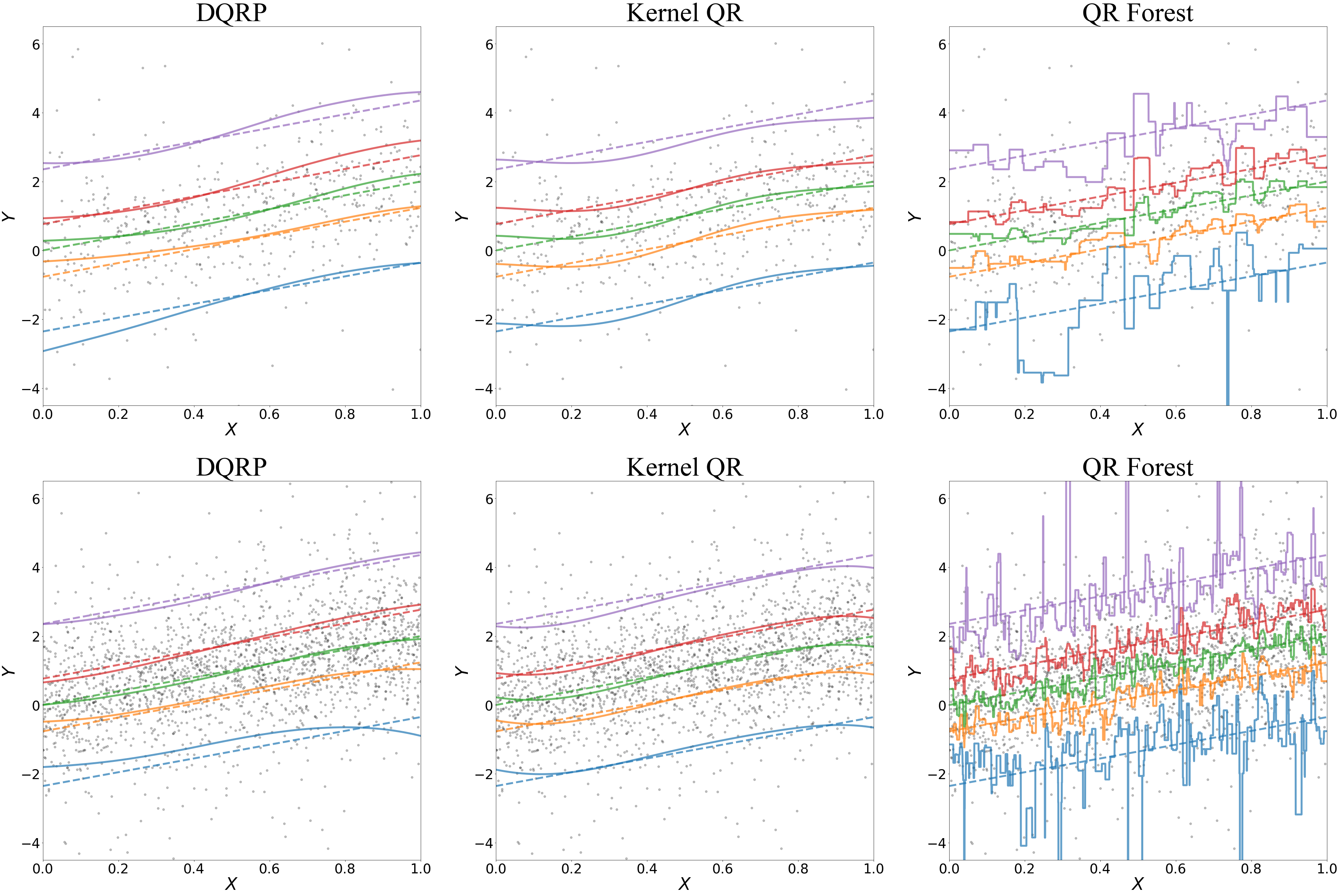
Figure 8: The fitted quantile curves by different methods under the univariate “Linear” model when $n=512,2048$. The training data is depicted as grey dots.The target quantile functions at the quantile levels $\tau=$0.05 (blue), 0.25 (orange), 0.5 (green), 0.75 (red), 0.95 (purple) are depicted as dashed curves, and the estimated quantile functions are represented by solid curves with the same color. From the top to the bottom, the rows correspond to the sample size $n=512,2048$. From the left to the right, the columns correspond to the methods DQRP, kernel QR and QR Forest.

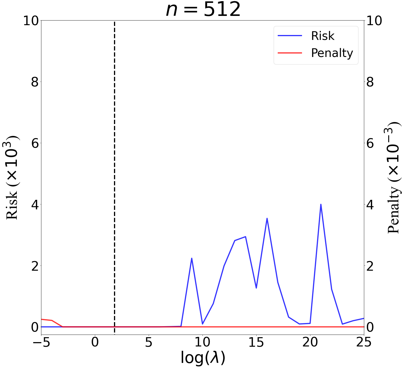
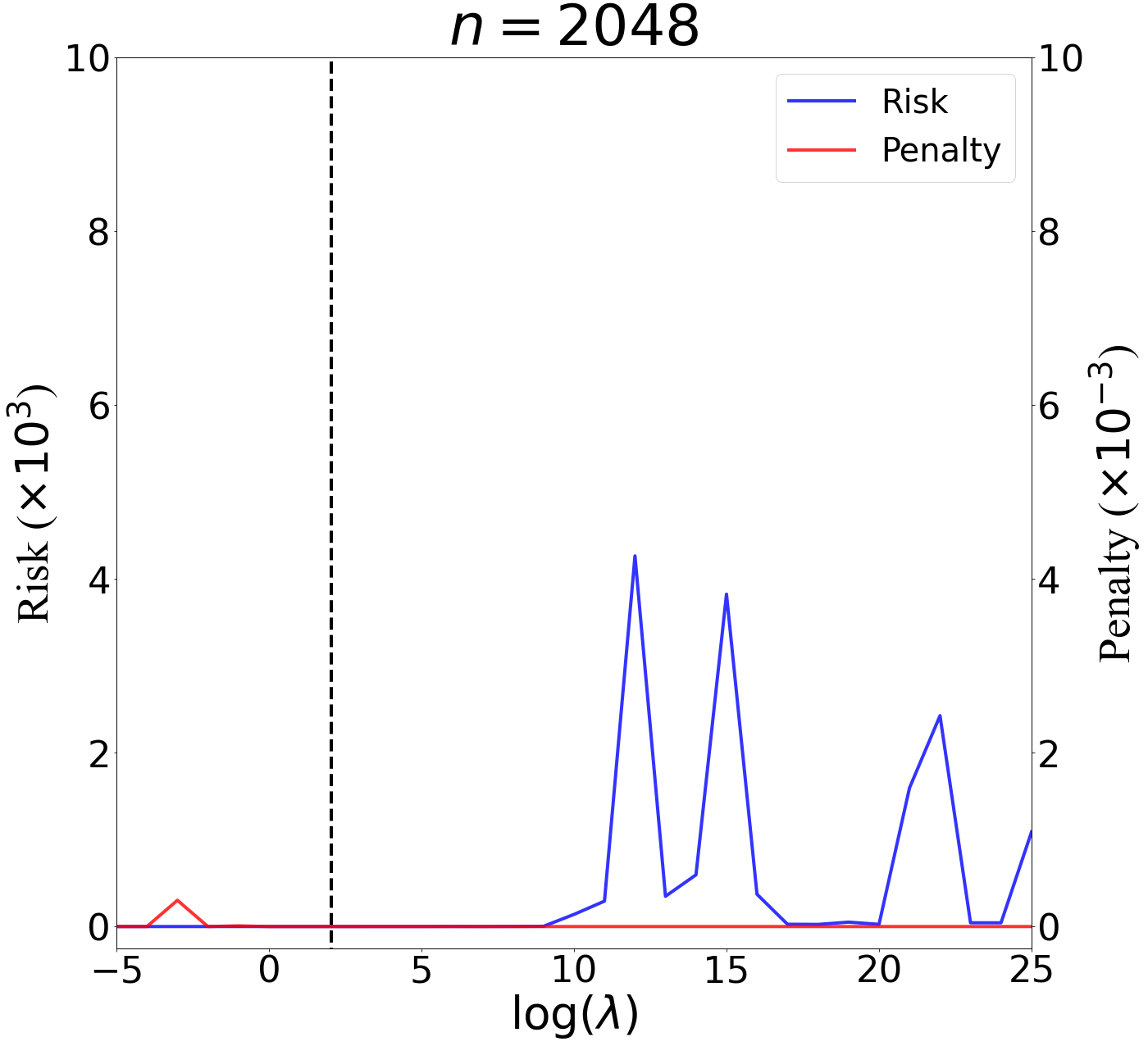
Figure 9: The value of risks and penalties under the univariate “Wave” model when $n=512,2048$. A vertical dashed line is depicted at the value $\lambda=\log(n)$ on x-axis in each figure.

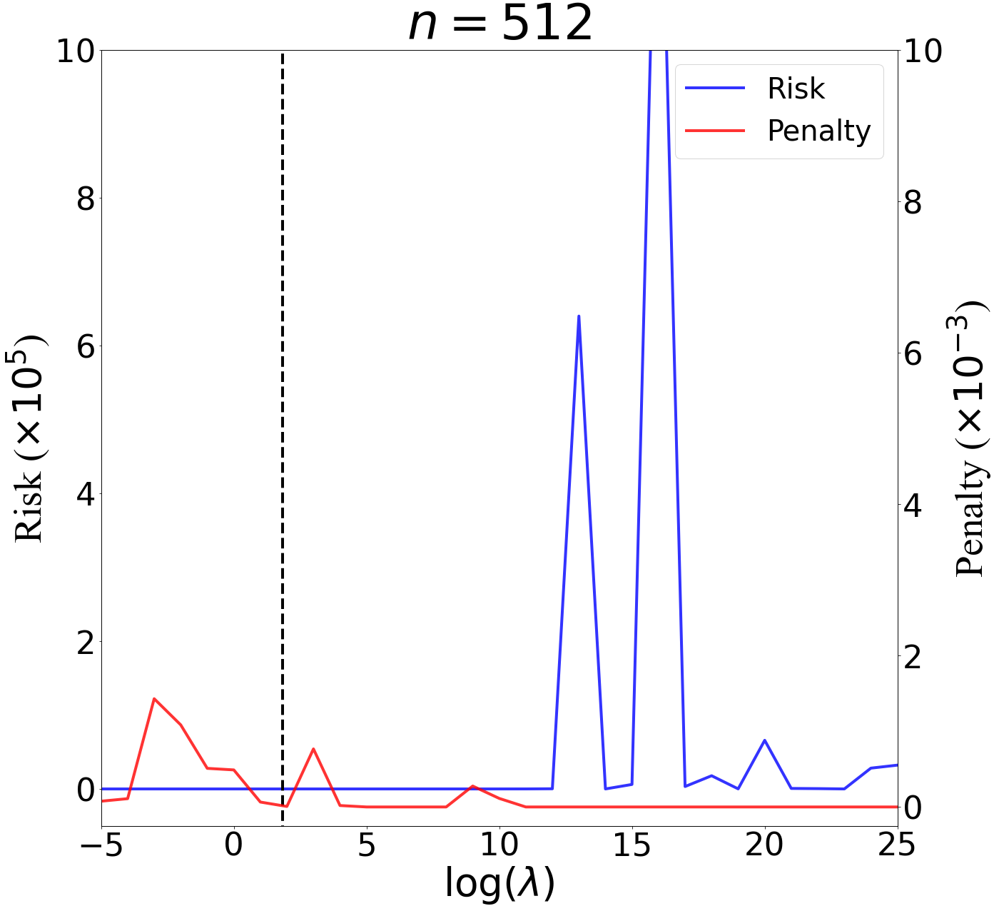
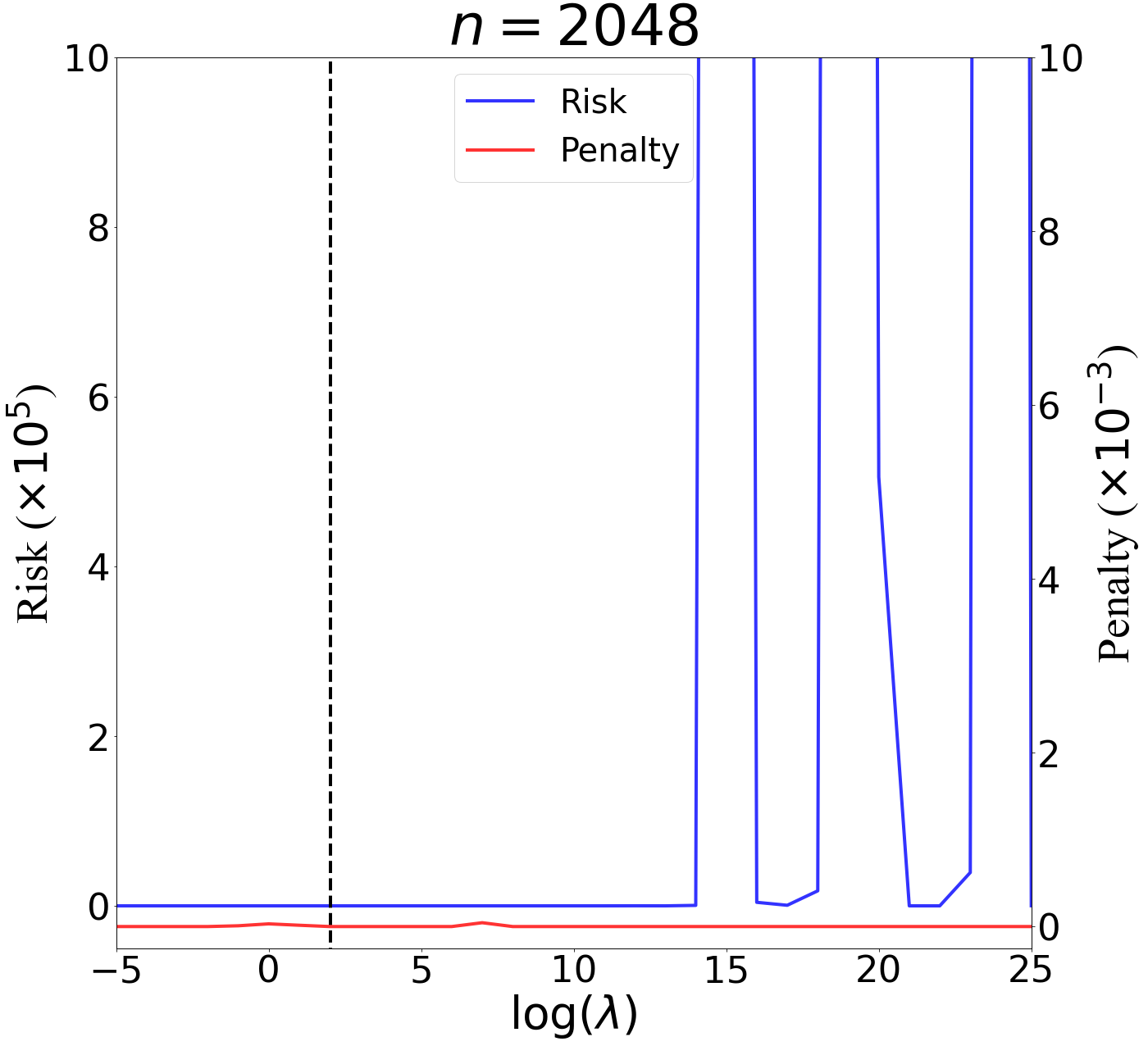
Figure 10: The value of risks and penalties under the multivariate single index model when $n=512,2048$ and $d=8$. A vertical dashed line is depicted at the value $\lambda=\log(n)$ on x-axis in each figure.

References

• Anthony and Bartlett (1999) {bbook}[author] \bauthor\bsnmAnthony, \bfnmMartin\binitsM. and \bauthor\bsnmBartlett, \bfnmPeter L.\binitsP. L. (\byear1999). \btitleNeural Network Learning: Theoretical Foundations. \bpublisherCambridge University Press, Cambridge. \bdoi10.1017/CBO9780511624216 \endbibitem
• Bachrach et al. (1999) {barticle}[author] \bauthor\bsnmBachrach, \bfnmLaura K\binitsL. K., \bauthor\bsnmHastie, \bfnmTrevor\binitsT., \bauthor\bsnmWang, \bfnmMay-Choo\binitsM.-C., \bauthor\bsnmNarasimhan, \bfnmBalasubramanian\binitsB. and \bauthor\bsnmMarcus, \bfnmRobert\binitsR. (\byear1999). \btitleBone mineral acquisition in healthy Asian, Hispanic, black, and Caucasian youth: a longitudinal study. \bjournalThe Journal of Clinical Endocrinology & Metabolism \bvolume84 \bpages4702–4712. \endbibitem
• Bagby, Bos and Levenberg (2002) {barticle}[author] \bauthor\bsnmBagby, \bfnmThomas\binitsT., \bauthor\bsnmBos, \bfnmLen\binitsL. and \bauthor\bsnmLevenberg, \bfnmNorman\binitsN. (\byear2002). \btitleMultivariate simultaneous approximation. \bjournalConstructive approximation \bvolume18 \bpages569–577. \endbibitem
• Bartlett et al. (2019) {barticle}[author] \bauthor\bsnmBartlett, \bfnmPeter L.\binitsP. L., \bauthor\bsnmHarvey, \bfnmNick\binitsN., \bauthor\bsnmLiaw, \bfnmChristopher\binitsC. and \bauthor\bsnmMehrabian, \bfnmAbbas\binitsA. (\byear2019). \btitleNearly-tight VC-dimension and pseudodimension bounds for piecewise linear neural networks. \bjournalJournal of Machine Learning Research \bvolume20 \bpagesPaper No. 63, 17. \endbibitem
• Bauer and Kohler (2019) {barticle}[author] \bauthor\bsnmBauer, \bfnmBenedikt\binitsB. and \bauthor\bsnmKohler, \bfnmMichael\binitsM. (\byear2019). \btitleOn deep learning as a remedy for the curse of dimensionality in nonparametric regression. \bjournalAnn. of Statist. \bvolume47 \bpages2261–2285. \bdoi10.1214/18-AOS1747 \endbibitem
• Belloni et al. (2011) {barticle}[author] \bauthor\bsnmBelloni, \bfnmAlexandre\binitsA., \bauthor\bsnmChernozhukov, \bfnmVictor\binitsV. \betalet al. (\byear2011). \btitle$\ell$1-penalized quantile regression in high-dimensional sparse models. \bjournalAnn. Statist. \bvolume39 \bpages82–130. \endbibitem
• Belloni et al. (2019) {barticle}[author] \bauthor\bsnmBelloni, \bfnmAlexandre\binitsA., \bauthor\bsnmChernozhukov, \bfnmVictor\binitsV., \bauthor\bsnmChetverikov, \bfnmDenis\binitsD. and \bauthor\bsnmFernandez-Val, \bfnmIvan\binitsI. (\byear2019). \btitleConditional quantile processes based on series or many regressors. \bjournalJournal of Econometrics \bvolume213 \bpages4-29. \endbibitem
• Blundell, Horowitz and Parey (2017) {barticle}[author] \bauthor\bsnmBlundell, \bfnmRichard\binitsR., \bauthor\bsnmHorowitz, \bfnmJoel\binitsJ. and \bauthor\bsnmParey, \bfnmMatthias\binitsM. (\byear2017). \btitleNonparametric estimation of a nonseparable demand function under the Slutsky inequality restriction. \bjournalThe Review of Economics and Statistics \bvolume99 \bpages291-304. \endbibitem
• Bondell, Reich and Wang (2010) {barticle}[author] \bauthor\bsnmBondell, \bfnmHoward D.\binitsH. D., \bauthor\bsnmReich, \bfnmBrian J.\binitsB. J. and \bauthor\bsnmWang, \bfnmHuixia\binitsH. (\byear2010). \btitleNoncrossing quantile regression curve estimation. \bjournalBiometrika \bvolume97 \bpages825-838. \bdoi10.1093/biomet/asq048 \endbibitem
• Brando et al. (2022) {barticle}[author] \bauthor\bsnmBrando, \bfnmAxel\binitsA., \bauthor\bsnmGimeno, \bfnmJoan\binitsJ., \bauthor\bsnmRodríguez-Serrano, \bfnmJose A\binitsJ. A. and \bauthor\bsnmVitrià, \bfnmJordi\binitsJ. (\byear2022). \btitleDeep non-crossing quantiles through the partial derivative. \bjournalarXiv preprint arXiv:2201.12848. \endbibitem
• Chao, Volgushev and Cheng (2016) {barticle}[author] \bauthor\bsnmChao, \bfnmShih-Kang\binitsS.-K., \bauthor\bsnmVolgushev, \bfnmStanislav\binitsS. and \bauthor\bsnmCheng, \bfnmGuang\binitsG. (\byear2016). \btitleQuantile Processes for Semi and Nonparametric Regression. \bjournalElectronic Journal of Statistics \bvolume11. \bdoi10.1214/17-EJS1313 \endbibitem
• Chen et al. (2019) {barticle}[author] \bauthor\bsnmChen, \bfnmMinshuo\binitsM., \bauthor\bsnmJiang, \bfnmHaoming\binitsH., \bauthor\bsnmLiao, \bfnmWenjing\binitsW. and \bauthor\bsnmZhao, \bfnmTuo\binitsT. (\byear2019). \btitleNonparametric regression on low-dimensional manifolds using deep relu networks. \bjournalarXiv preprint arXiv:1908.01842. \endbibitem
• Chernozhukov, Fernández-Val and Galichon (2010) {barticle}[author] \bauthor\bsnmChernozhukov, \bfnmVictor\binitsV., \bauthor\bsnmFernández-Val, \bfnmIván\binitsI. and \bauthor\bsnmGalichon, \bfnmAlfred\binitsA. (\byear2010). \btitleQuantile and probability curves without crossing. \bjournalEconometrica \bvolume78 \bpages1093–1125. \endbibitem
• Chernozhukov and Hansen (2005) {barticle}[author] \bauthor\bsnmChernozhukov, \bfnmVictor\binitsV. and \bauthor\bsnmHansen, \bfnmChristian\binitsC. (\byear2005). \btitleAn IV model of quantile treatment effects. \bjournalEconometrica \bvolume73 \bpages245-261. \endbibitem
• Chernozhukov, Imbens and Newey (2007) {barticle}[author] \bauthor\bsnmChernozhukov, \bfnmVictor\binitsV., \bauthor\bsnmImbens, \bfnmGuido W.\binitsG. W. and \bauthor\bsnmNewey, \bfnmWhitney K.\binitsW. K. (\byear2007). \btitleInstrumental variable estimation of nonseparable models. \bjournalJournal of Econometrics \bvolume139 \bpages4-14. \bdoi10.1016/j.jeconom.2006.06.002 \endbibitem
• Duan et al. (2021) {barticle}[author] \bauthor\bsnmDuan, \bfnmChenguang\binitsC., \bauthor\bsnmJiao, \bfnmYuling\binitsY., \bauthor\bsnmLai, \bfnmYanming\binitsY., \bauthor\bsnmLu, \bfnmXiliang\binitsX. and \bauthor\bsnmYang, \bfnmZhijian\binitsZ. (\byear2021). \btitleConvergence rate analysis for deep ritz method. \bjournalarXiv preprint arXiv:2103.13330. \endbibitem
• Farrell, Liang and Misra (2021) {barticle}[author] \bauthor\bsnmFarrell, \bfnmMax H.\binitsM. H., \bauthor\bsnmLiang, \bfnmTengyuan\binitsT. and \bauthor\bsnmMisra, \bfnmSanjog\binitsS. (\byear2021). \btitleDeep neural networks for estimation and inference. \bjournalEconometrica \bvolume89 \bpages181–213. \bdoi10.3982/ecta16901 \endbibitem
• Fercoq and Bianchi (2019) {barticle}[author] \bauthor\bsnmFercoq, \bfnmOlivier\binitsO. and \bauthor\bsnmBianchi, \bfnmPascal\binitsP. (\byear2019). \btitleA coordinate-descent primal-dual algorithm with large step size and possibly nonseparable functions. \bjournalSIAM Journal on Optimization \bvolume29 \bpages100–134. \endbibitem
• Goldberg and Jerrum (1995) {barticle}[author] \bauthor\bsnmGoldberg, \bfnmPaul W\binitsP. W. and \bauthor\bsnmJerrum, \bfnmMark R\binitsM. R. (\byear1995). \btitleBounding the Vapnik-Chervonenkis dimension of concept classes parameterized by real numbers. \bjournalMachine Learning \bvolume18 \bpages131–148. \endbibitem
• Hastie et al. (2009) {bbook}[author] \bauthor\bsnmHastie, \bfnmTrevor\binitsT., \bauthor\bsnmTibshirani, \bfnmRobert\binitsR., \bauthor\bsnmFriedman, \bfnmJerome H\binitsJ. H. and \bauthor\bsnmFriedman, \bfnmJerome H\binitsJ. H. (\byear2009). \btitleThe elements of statistical learning: data mining, inference, and prediction \bvolume2. \bpublisherSpringer. \endbibitem
• He (1997) {barticle}[author] \bauthor\bsnmHe, \bfnmXuming\binitsX. (\byear1997). \btitleQuantile curves without crossing. \bjournalThe American Statistician \bvolume51 \bpages186-192. \bdoi10.1080/00031305.1997.10473959 \endbibitem
• He and Ng (1999) {barticle}[author] \bauthor\bsnmHe, \bfnmXuming\binitsX. and \bauthor\bsnmNg, \bfnmPin\binitsP. (\byear1999). \btitleQuantile splines with several covariates. \bjournalJournal of Statistical Planning and Inference \bvolume75 \bpages343–352. \endbibitem
• He and Shi (1994) {barticle}[author] \bauthor\bsnmHe, \bfnmXuming\binitsX. and \bauthor\bsnmShi, \bfnmPeide\binitsP. (\byear1994). \btitleConvergence rate of B-spline estimators of nonparametric conditional quantile functions. \bjournalJournaltitle of Nonparametric Statistics \bvolume3 \bpages299–308. \endbibitem
• Hörmander (2015) {bbook}[author] \bauthor\bsnmHörmander, \bfnmLars\binitsL. (\byear2015). \btitleThe Analysis of Linear Partial Differential Operators I: Distribution Theory and Fourier Analysis. \bpublisherSpringer. \endbibitem
• Horowitz and Lee (2007) {barticle}[author] \bauthor\bsnmHorowitz, \bfnmJoel L.\binitsJ. L. and \bauthor\bsnmLee, \bfnmSokbae\binitsS. (\byear2007). \btitleNonparametric instrumental variables estimation of a quantile regression model. \bjournalEconometrica \bvolume75 \bpages1191-1208. \endbibitem
• Jiao et al. (2021) {barticle}[author] \bauthor\bsnmJiao, \bfnmYuling\binitsY., \bauthor\bsnmShen, \bfnmGuohao\binitsG., \bauthor\bsnmLin, \bfnmYuanyuan\binitsY. and \bauthor\bsnmHuang, \bfnmJian\binitsJ. (\byear2021). \btitleDeep nonparametric regression on approximately low-dimensional manifolds. \bjournalarXiv 2104.06708. \endbibitem
• Kingma and Ba (2014) {barticle}[author] \bauthor\bsnmKingma, \bfnmDiederik P\binitsD. P. and \bauthor\bsnmBa, \bfnmJimmy\binitsJ. (\byear2014). \btitleAdam: A method for stochastic optimization. \bjournalarXiv preprint arXiv:1412.6980. \endbibitem
• Koenker (2005) {bbook}[author] \bauthor\bsnmKoenker, \bfnmR.\binitsR. (\byear2005). \btitleQuantile Regression. \bpublisherCambridge University Press. \endbibitem
• Koenker and Bassett (1978) {barticle}[author] \bauthor\bsnmKoenker, \bfnmR.\binitsR. and \bauthor\bsnmBassett, \bfnmG.\binitsG. (\byear1978). \btitleRegression quantiles. \bjournalEconometrica \bvolume46 \bpages33–50. \endbibitem
• Koenker, Ng and Portnoy (1994) {barticle}[author] \bauthor\bsnmKoenker, \bfnmR.\binitsR., \bauthor\bsnmNg, \bfnmP.\binitsP. and \bauthor\bsnmPortnoy, \bfnmS.\binitsS. (\byear1994). \btitleQuantile smoothing splines. \bjournalBiometrica \bvolume81 \bpages673–680. \endbibitem
• Kohler, Krzyzak and Langer (2019) {barticle}[author] \bauthor\bsnmKohler, \bfnmMichael\binitsM., \bauthor\bsnmKrzyzak, \bfnmAdam\binitsA. and \bauthor\bsnmLanger, \bfnmSophie\binitsS. (\byear2019). \btitleEstimation of a function of low local dimensionality by deep neural networks. \bjournalarXiv preprint arXiv:1908.11140. \endbibitem
• Ledoux and Talagrand (1991) {bbook}[author] \bauthor\bsnmLedoux, \bfnmMichel\binitsM. and \bauthor\bsnmTalagrand, \bfnmMichel\binitsM. (\byear1991). \btitleProbability in Banach Spaces: Isoperimetry and Processes \bvolume23. \bpublisherSpringer Science & Business Media. \endbibitem
• Li, Tang and Yu (2019a) {barticle}[author] \bauthor\bsnmLi, \bfnmBo\binitsB., \bauthor\bsnmTang, \bfnmShanshan\binitsS. and \bauthor\bsnmYu, \bfnmHaijun\binitsH. (\byear2019a). \btitlePowerNet: Efficient representations of polynomials and smooth functions by deep neural networks with rectified power units. \bjournalarXiv preprint arXiv:1909.05136. \endbibitem
• Li, Tang and Yu (2019b) {barticle}[author] \bauthor\bsnmLi, \bfnmBo\binitsB., \bauthor\bsnmTang, \bfnmShanshan\binitsS. and \bauthor\bsnmYu, \bfnmHaijun\binitsH. (\byear2019b). \btitleBetter approximations of high dimensional smooth functions by deep neural networks with rectified power units. \bjournalarXiv preprint arXiv:1903.05858. \endbibitem
• Lu et al. (2021) {barticle}[author] \bauthor\bsnmLu, \bfnmJianfeng\binitsJ., \bauthor\bsnmShen, \bfnmZuowei\binitsZ., \bauthor\bsnmYang, \bfnmHaizhao\binitsH. and \bauthor\bsnmZhang, \bfnmShijun\binitsS. (\byear2021). \btitleDeep network approximation for smooth functions. \bjournalSIAM Journal on Mathematical Analysis \bvolume53 \bpages5465–5506. \endbibitem
• Mammen (1991) {barticle}[author] \bauthor\bsnmMammen, \bfnmEnno\binitsE. (\byear1991). \btitleNonparametric regression under qualitative smoothness assumptions. \bjournalThe Annals of Statistics \bvolume19 \bpages741 – 759. \bdoi10.1214/aos/1176348118 \endbibitem
• Meinshausen and Ridgeway (2006) {barticle}[author] \bauthor\bsnmMeinshausen, \bfnmNicolai\binitsN. and \bauthor\bsnmRidgeway, \bfnmGreg\binitsG. (\byear2006). \btitleQuantile regression forests. \bjournalJournal of Machine Learning Research \bvolume7. \endbibitem
• Nakada and Imaizumi (2020) {barticle}[author] \bauthor\bsnmNakada, \bfnmRyumei\binitsR. and \bauthor\bsnmImaizumi, \bfnmMasaaki\binitsM. (\byear2020). \btitleAdaptive approximation and estimation of deep neural network with intrinsic dimensionality. \bjournalJournal of Machine Learning Research \bvolume21 \bpages1–38. \endbibitem
• Padilla and Chatterjee (2021) {barticle}[author] \bauthor\bsnmPadilla, \bfnmOscar Hernan Madrid\binitsO. H. M. and \bauthor\bsnmChatterjee, \bfnmSabyasachi\binitsS. (\byear2021). \btitleRisk bounds for quantile trend filtering. \bjournalarXiv preprint arXiv:2007.07472v5. \endbibitem
• Sangnier, Fercoq and d’Alché Buc (2016) {barticle}[author] \bauthor\bsnmSangnier, \bfnmMaxime\binitsM., \bauthor\bsnmFercoq, \bfnmOlivier\binitsO. and \bauthor\bparticled’Alché \bsnmBuc, \bfnmFlorence\binitsF. (\byear2016). \btitleJoint quantile regression in vector-valued RKHSs. \bjournalAdvances in Neural Information Processing Systems \bvolume29 \bpages3693–3701. \endbibitem
• Schmidt-Hieber et al. (2020) {barticle}[author] \bauthor\bsnmSchmidt-Hieber, \bfnmJohannes\binitsJ. \betalet al. (\byear2020). \btitleNonparametric regression using deep neural networks with ReLU activation function. \bjournalAnnals of Statistics \bvolume48 \bpages1875–1897. \endbibitem
• Shen, Yang and Zhang (2019) {barticle}[author] \bauthor\bsnmShen, \bfnmZuowei\binitsZ., \bauthor\bsnmYang, \bfnmHaizhao\binitsH. and \bauthor\bsnmZhang, \bfnmShijun\binitsS. (\byear2019). \btitleNonlinear approximation via compositions. \bjournalNeural Networks \bvolume119 \bpages74–84. \endbibitem
• Shen, Yang and Zhang (2020) {barticle}[author] \bauthor\bsnmShen, \bfnmZuowei\binitsZ., \bauthor\bsnmYang, \bfnmHaizhao\binitsH. and \bauthor\bsnmZhang, \bfnmShijun\binitsS. (\byear2020). \btitleDeep network approximation characterized by number of neurons. \bjournalCommun. Comput. Phys. \bvolume28 \bpages1768–1811. \bdoi10.4208/cicp.oa-2020-0149 \endbibitem
• Shen et al. (2021) {barticle}[author] \bauthor\bsnmShen, \bfnmGuohao\binitsG., \bauthor\bsnmJiao, \bfnmYuling\binitsY., \bauthor\bsnmLin, \bfnmYuanyuan\binitsY., \bauthor\bsnmHorowitz, \bfnmJoel L\binitsJ. L. and \bauthor\bsnmHuang, \bfnmJian\binitsJ. (\byear2021). \btitleDeep quantile regression: mitigating the curse of dimensionality through composition. \bjournalarXiv preprint arXiv:2107.04907. \endbibitem
• Steinwart (2007) {barticle}[author] \bauthor\bsnmSteinwart, \bfnmIngo\binitsI. (\byear2007). \btitleHow to compare different loss functions and their risks. \bjournalConstructive Approximation \bvolume26 \bpages225–287. \endbibitem
• Takeuchi et al. (2006) {barticle}[author] \bauthor\bsnmTakeuchi, \bfnmIchiro\binitsI., \bauthor\bsnmLe, \bfnmQuoc V.\binitsQ. V., \bauthor\bsnmSears, \bfnmTimothy D.\binitsT. D. and \bauthor\bsnmSmola, \bfnmAlexander J.\binitsA. J. (\byear2006). \btitleNonparametric quantile estimation. \bjournalJournal of Machine Learning Research \bvolume7 \bpages1231-1264. \endbibitem
• Wang, Wu and Li (2012) {barticle}[author] \bauthor\bsnmWang, \bfnmLan\binitsL., \bauthor\bsnmWu, \bfnmYichao\binitsY. and \bauthor\bsnmLi, \bfnmRunze\binitsR. (\byear2012). \btitleQuantile regression for analyzing heterogeneity in ultra-high dimension. \bjournalJournal of the American Statistical Association \bvolume107 \bpages214–222. \endbibitem
• White (1992) {bincollection}[author] \bauthor\bsnmWhite, \bfnmHalbert\binitsH. (\byear1992). \btitleNonparametric estimation of conditional quantiles using neural networks. In \bbooktitleComputing Science and Statistics \bpages190–199. \bpublisherSpringer. \endbibitem
• Yarotsky (2017) {barticle}[author] \bauthor\bsnmYarotsky, \bfnmDmitry\binitsD. (\byear2017). \btitleError bounds for approximations with deep ReLU networks. \bjournalNeural Networks \bvolume94 \bpages103–114. \endbibitem
• Yarotsky (2018) {binproceedings}[author] \bauthor\bsnmYarotsky, \bfnmDmitry\binitsD. (\byear2018). \btitleOptimal approximation of continuous functions by very deep ReLU networks. In \bbooktitleConference on Learning Theory \bpages639–649. \bpublisherPMLR. \endbibitem
• Zheng, Peng and He (2015) {barticle}[author] \bauthor\bsnmZheng, \bfnmQi\binitsQ., \bauthor\bsnmPeng, \bfnmLimin\binitsL. and \bauthor\bsnmHe, \bfnmXuming\binitsX. (\byear2015). \btitleGlobally adaptive quantile regression with ultra-high dimensional data. \bjournalAnn. Statist. \bvolume43 \bpages2225–2258. \endbibitem