High-Harmonic Spectroscopy of Coherent Lattice Dynamics in Graphene

Abstract

High-harmonic spectroscopy of solids is a powerful tool, which provides access to both electronic structure and ultrafast electronic response of solids, from their band structure and density of states, to phase transitions, including the emergence of the topological edge states, to the PetaHertz electronic response. However, in spite of these successes, high harmonic spectroscopy has hardly been applied to analyse the role of coherent femtosecond lattice vibrations in the attosecond electronic response. Here we study coherent phonon excitations in monolayer graphene to show how high-harmonic spectroscopy can be used to detect the influence of coherent lattice dynamics, particularly longitudinal and transverse optical phonon modes, on the electronic response. Coherent excitation of the in-plane phonon modes results in the appearance of sidebands in the spectrum of the emitted harmonic radiation. We show that the spectral positions and the polarisation of the sideband emission offer a sensitive probe of the dynamical symmetries associated with the excited phonon modes. Our work brings the key advantage of high harmonic spectroscopy – the combination of sub-femtosecond to tens of femtoseconds temporal resolution – to the problem of probing phonon-driven electronic response and its dependence on the dynamical symmetries in solids.

I Introduction

Strong-field driven high-harmonic generation (HHG) is a nonlinear frequency up-conversion process, which emits radiation at integer multiples of the incident laser frequency Ferray et al. (1988). Taking advantage of major technical advances in mid-infrared sources, the pioneering experiments Ghimire et al. (2011) have extended HHG from gases to solids, stimulating intense research into probing electron dynamics in solids on the natural timescale. Today, high-harmonic spectroscopy has been employed to probe different static and dynamic properties of solids, such as band dispersion Vampa et al. (2015); Luu et al. (2015); Lanin et al. (2017); Mrudul et al. (2019), density of states Tancogne-Dejean et al. (2017), band defects Mrudul et al. (2020); Pattanayak et al. (2020), valley pseudospin Mrudul et al. (2021); Jiménez-Galán et al. (2020); Langer et al. (2018); Mrudul and Dixit (2021a), Bloch oscillations Schubert et al. (2014), topology and light-driven phase transitions, including strongly correlated systems  Bauer and Hansen (2018); Silva et al. (2018); Bai et al. (2020); Imai et al. (2020); Borsch et al. (2020); Baykusheva et al. (2021); Bharti et al. (2022); Pattanayak et al. (2022); Chacón et al. (2020); Shao et al. (2022), and even combine attosecond temporal with pico-meter spatial resolution of electron trajectories in lattices Lakhotia et al. (2020).

Availability of mid-infrared light sources also enables coherent excitation of a desired phonon mode by tuning the polarisation and frequency of the laser pulse  Mankowsky et al. (2016). Yet, the analysis of the effect of coherent lattice dynamics on high harmonic generation in solids appears lacking, apart from a lone experiment Hollinger et al. (2019). This situation stands in stark contrast to molecular gases, where high-harmonic spectroscopy has been extensively employed to probe nuclear motion in various molecules Patchkovskii (2009); Wagner et al. (2006); Le et al. (2012); Baker et al. (2006); Lein (2005); Wörner et al. (2011). Present work aims to fill this gap and highlight some of the capabilities offered by high harmonic spectroscopy in time-resolving the interplay of femtosecond lattice and attosecond electronic motions. Such interplay is essential for many fundamental phenomena, including thermal conductivity Niedziela et al. (2019), optical reflectivity Dove (1993); Katsuki et al. (2013), structural phase transition Bansal et al. (2020); Hase et al. (2015), heat capacity Bansal et al. (2018), and optical properties Fultz (2010); Gambetta et al. (2006).

Various spectroscopic methods have been developed to excite and probe phonons, see e.g.  Dhar et al. (1994); Debnath et al. (2021); Graf et al. (2007); Virga et al. (2019); Koivistoinen et al. (2017); Rana et al. (2021); Brown et al. (2019); Flannigan (2018); Gierz et al. (2015); Moulet et al. (2017); Géneaux et al. (2020), but their temporal resolution is limited by the length of the pulses used. Large coherent bandwidth of high harmonic signals offers sub-laser-cycle temporal resolution and the possibility to time-resolve the impact of lattice distortions on the faster electronic response.

One difficulty in tracking lattice vibrations via highly nonlinear optical response stems from their small amplitude. If the corresponding changes in both the band structure and couplings are similarly small, the high-harmonic response hardly changes. Yet, large distortions are not needed if the excited phonon mode dynamically changes the symmetry of the unit cell. Here we show how coherent phonon dynamics and the associated changes in the lattice symmetry are encoded in the electronic response and the harmonic signal, and how the sub-cycle temporal resolution inherent in the harmonic signal can be used to track the interplay of electronic and lattice dynamics.

Figure 1: Hexagonal honeycomb structure of graphene and associated in-plane phonon modes. (a) Real-space structure of graphene. (b) Brillouin zone in momentum-space with $\mathsf{\Gamma,M,}$ and $\mathsf{K}$ as the high symmetry points. (c) and (d) are the sketches of atomic vibrations associated with the degenerate E_2g phonon modes in real-space. Here, modes are labelled as (c) in-plane longitudinal optical (iLO) phonon mode and (d) in-plane transverse optical (iTO) phonon mode, respectively.

We analyse monolayer graphene, which belongs to $\textbf{D}_{6h}$ point group symmetry, see Fig. 1(a). It exhibits six phonon branches: three optical and three acoustic. Here we focus on the former. Out of the three optical phonon modes, one is out-of-plane, the two others are in-plane modes. We will consider only the in-plane modes. The lattice vibrations corresponding to the in-plane Longitudinal Optical (iLO), and the in-plane Transverse Optical (iTO) E_2g modes are shown in Fig. 1(c) and 1(d), respectively. The two modes are degenerate at the $\mathsf{\Gamma}$-point, with the phonon frequency equal to 194 meV (oscillation period $\sim$ 21 femtoseconds Kim et al. (2013)); both are Raman active and can be excited with a resonant pulse pair or impulsively by a short pulse with bandwidth covering 194 meV. Moreover, it is possible to selectively excite either iLO or iTO coherent phonon mode by tuning the polarisation of the pump pulse either along $\mathsf{\Gamma-K}$ or $\mathsf{\Gamma-M}$ direction, respectively.

Coherent lattice dynamics should in general introduce periodic modulations of the system parameters and thus of its high-harmonic response. In the frequency domain, such modulations add sidebands to the main peaks in the harmonic spectrum. We shall see that their position and polarisation encode the information about the frequency and the symmetry of the excited phonon mode, respectively.

II Theoretical Method

Carbon atoms are arranged at the corners of a hexagon in the honeycomb lattice of the graphene. The unit-cell of graphene has a two-atom basis, usually denoted as A and B atoms. The corresponding Brillouin zone in momentum space is shown in Fig. 1(b), where $\mathsf{\Gamma}$, $\mathsf{M}$, and $\mathsf{K}$ are the high-symmetry points. In our convention, the zigzag and armchair directions of graphene are along $\mathsf{X}$-axis ($\mathsf{\Gamma}-\mathsf{K}$ direction) and $\mathsf{Y}$-axis ($\mathsf{\Gamma}-\mathsf{M}$ direction), respectively.

The electronic ground-state of the graphene is described by the nearest-neighbour tight-binding approximation and the corresponding Hamiltonian is written as

$$\mathcal{\hat{H}}_{\textbf{k}}=-\gamma_{0}\sum_{i\in nn}~{}e^{i\textbf{k}\cdot\textbf{d}_{i}}\hat{a}_{\textbf{k}}^{\dagger}\hat{b}_{\textbf{k}}+\textrm{H. c.}$$ (1)

Here, the summation is over the nearest neighbour atoms. $\gamma_{0}$ is the nearest-neighbour hopping energy, which is chosen to be 2.7 eV. $\textbf{d}_{i}$ is the separation vector between an atom with its nearest neighbour, such that $|\textbf{d}_{i}|=a$ = 1.42 Å is the inter-atomic distance, for a lattice parameter $a_{0}$ of 2.46 Å. $\hat{a}_{k}^{\dagger}(\hat{b}_{k})$ is creation (annihilation) operator for atom A (B) in the unit cell. The low-energy band-structure of graphene is obtained by solving Eq. (1) and has zero band-gap and exhibits linear dispersion at $\mathsf{K}$-points in the Brillouin zone.

We treat lattice dynamics classically, and assume that atoms perform harmonic oscillations for short displacements from their equilibrium positions. The displacement vector for a particular phonon mode is expressed as

$$\textbf{q}(t)=\textrm{q}_{0}~{}\hat{\textbf{e}}~{}\rm{Re}\left(e^{i\omega_{ph}t}\right).$$ (2)

Here, $\textrm{q}_{0}$ is the maximum displacement of an atom from its equilibrium position, $\omega_{\textrm{ph}}=$ 194 meV is the energy of the E_2g phonon mode , and $\hat{\textbf{e}}$ is the normalised eigenvector for a particular phonon mode. From Figs. 1(c) and 1(d), it is clear that $\hat{\textbf{e}}_{\textsf{iLO}}$ = $[1,0,-1,0]/\sqrt{2}$ and $\hat{\textbf{e}}_{\textsf{iTO}}$ = $[0,1,0,-1]/\sqrt{2}$, in which the first (last) two elements are components of A (B) atom.

Due to coherent phonon excitations, lattice dynamics causes temporal variations in the relative distance between atoms ($\textbf{d}_{i}$). In this case, the corresponding time-dependent Hamiltonian within the tight-binding approximation can be written as Mohanty and Heller (2019); Rodriguez-Vega et al. (2021); Wang and Fischer (2014)

$$\mathcal{\hat{H}}_{\textbf{k}}(t)=-\gamma(t)\sum_{i\in nn}e^{i\textbf{k}\cdot\textbf{d}_{i}(t)}\hat{a}_{\textbf{k}}^{\dagger}\hat{b}_{\textbf{k}}+\textrm{H. c.}$$ (3)

Here, the hopping energy is modelled as an exponentially decaying function of the relative displacement between nearest-neighbour atoms as $\gamma(t)$ = $\gamma_{0}~{}e^{-(|\textbf{d}_{i}(t)|-a)/\delta}$, in which $\delta$ is the width of the decay function chosen to be 0.184$a_{0}$ Moon and Koshino (2013).

The interaction among laser, electrons and coherently excited phonon mode in graphene is modelled by solving following equations of the single-particle density matrix. By updating the modified Hamiltonian as a result of the lattice dynamics, semiconductor Bloch equations in co-moving frame $|n,\textbf{k}+\textbf{A}(t)\rangle$, is extended and equations of motion read as

$$\frac{d}{dt}\rho_{vv}^{\textbf{k}} =i\textbf{E}(t)\cdot\textbf{d}_{vc}(\textbf{k}_{t},t)\rho_{cv}^{\textbf{k}}+\textrm{c.c.}$$ (4a)

$$\frac{d}{dt}\rho_{cv}^{\textbf{k}} =\left[-i\varepsilon_{cv}(\textbf{k}_{t},t)-\frac{1}{T_{2}}\right]\rho_{cv}^{\textbf{k}}+i\textbf{E}(t)\cdot\textbf{d}_{cv}(\textbf{k}_{t},t)\left[\rho_{vv}^{\textbf{k}}-\rho_{cc}^{\textbf{k}}\right].$$ (4b)

Here, $\textbf{E}(t)$ and $\textbf{A}(t)$ are, respectively, the electric field and the vector potential corresponding to the laser field, which are related as $\textbf{E}(t)$ = $-d\textbf{A}(t)/dt$, and $\textbf{k}_{t}$ is the shorthand notation for $\textbf{k}+\textbf{A}(t)$. $\varepsilon_{cv}(\textbf{k})$ and $\textbf{d}_{cv}(\textbf{k})$ are, respectively, the band-gap energy and dipole matrix elements between valence and conduction bands at k. $\textbf{d}_{cv}(\textbf{k})$ is defined as $\textbf{d}_{cv}(\textbf{k})=i\langle c,\textbf{k}|\nabla_{\textbf{k}}|v,\textbf{k}\rangle$. Also, $\rho_{cc}^{\textbf{k}}(t)=1-\rho_{vv}^{\textbf{k}}(t)$, and $\rho^{\textbf{k}}_{vc}(t)=\rho^{\textbf{k}*}_{cv}(t)$.

A phenomenological term to take care of the interband decoherence is added with a constant dephasing time $T_{2}$. We calculate the matrix elements at each time-step during temporal evolution of the coherently excited phonon mode, which results in the additional time-dependence in the matrix elements. As long as the maximum displacement of the atoms are small and the time-step is too small compared to the phonon time-period, the matrix elements at consecutive time-steps are smoothly updated.

We solve the coupled differential equations described in Eq. (4) using the fourth-order Runge-Kutta method with a time-step of 0.01 fs. We sampled the Brillouin zone with 251$\times$251 grid. The current at any k point in the Brillouin zone is defined as

$$\textbf{J}(\textbf{k},t)=\sum_{m,n\in\{c,v\}}\rho_{mn}^{\textbf{k}}(t)\textbf{p}_{nm}(\textbf{k}_{t},t).$$ (5)

Here, $\textbf{p}_{nm}$ are the momentum matrix-elements defined as $\textbf{p}_{nm}(\textbf{k})=\langle n,\textbf{k}|\nabla_{\textbf{{k}}}\mathcal{\hat{H}}_{\textbf{k}}|m,\textbf{k}\rangle$. The total current, J(t) can be calculated by integrating $\textbf{J}(\textbf{k},t)$ over the entire Brillouin zone.

The high-harmonic spectrum is simulated as

$$\mathcal{I}(\omega)=\left|\mathcal{FT}\left(\dfrac{\rm{d}}{{\rm d}t}\textbf{J}(t)\right)\right|^{2}.$$ (6)

Here, $\mathcal{FT}$ stands for the Fourier transform.

High-order harmonics are generated from monolayer graphene, with or without coherent lattice dynamics, using a linearly polarised pulse with a wavelength of 2.0 $\mu$m and peak intensity of 1$\times 10^{11}$ W/cm². The pulse is 100 fs long and has a sin-squared envelope. The laser parameters used in this work are below the damage threshold of graphene Currie et al. (2011). Similar laser parameters have been used to investigate electron dynamics in graphene via intense laser pulse  Heide et al. (2018); Higuchi et al. (2017); Yoshikawa et al. (2017). The value of the dephasing time $T_{2}=$ 10 fs is used throughout in this work Mrudul and Dixit (2021b). The observations we made here are consistent for other values of $T_{2}$ in the range 5 - 30 fs. Both in-plane E_2g phonon modes are considered here. Results presented in this work correspond to a maximum 0.03a₀ displacement of atoms from their equilibrium positions during coherent lattice dynamics. However, our findings remain valid for displacements ranging from 0.01a₀ to 0.05a₀ with respect to the equilibrium positions.

III Results and Discussion

High-harmonic spectra for monolayer graphene, with and without coherent lattice dynamics, are presented in Fig. 2. The spectrum corresponding to the graphene, without lattice dynamics, is shown by grey shaded area as a reference. Owing to the inversion symmetry of the graphene, the reference spectrum in grey colour exhibits only odd harmonics (consistent with earlier reports, e.g. Refs. Mrudul and Dixit (2021b); Yoshikawa et al. (2017); Al-Naib et al. (2014).)

We assume that coherent phonon dynamics is excited prior to a high harmonic probe. When one of the E_2g phonon modes in graphene is coherently excited, the harmonic spectra display sidebands along with the main odd harmonic peaks as reflected from Fig. 2. The energy difference between the adjacent sidebands matches the phonon energy ($\omega_{\textrm{ph}}$). The sideband intensity is sensitive to the phonon amplitude but is clearly visible already for amplitudes above 0.01 of the lattice constant. Here we present the case of the amplitude equal to 0.03 of the lattice constant.

Figure 2: High-harmonic spectra of monolayer graphene with and without coherent lattice dynamics. (a) and (c) High-harmonic spectra corresponding to the coherent iLO E_2g phonon mode and the probe harmonic pulse is polarised along $\mathsf{\Gamma K}$ and $\mathsf{\Gamma M}$ directions, respectively. (b) and (d) Same as (a) and (c) except iTO E_2g phonon mode is coherently excited. In all the cases, sidebands corresponding to the first harmonic are marked at frequencies ($\omega_{0}\pm m\omega_{\textrm{ph}}$), where $\omega_{0}$ is the frequency of the harmonic generating probe pulse, and $\omega_{\textrm{ph}}$ is phonon frequency. The harmonics with grey shaded area are the reference spectra and represent the spectra of graphene without phonon excitation. The unit cell of the graphene with the corresponding phonon eigenvector and polarisation of the harmonic generating probe pulse are shown in the respective insets. Red (blue) colour corresponds the polarisation of emitted radiation parallel (perpendicular) to the polarisation of harmonic generating probe pulse.

As E_2g phonon modes preserve inversion centre, only odd harmonics are generated. When the coherent iLO mode and the probe harmonic pulse (along $\mathsf{\Gamma-K}$) are in the same direction, the even-oder sidebands are polarised along $\mathsf{\Gamma-K}$ (red colour), whereas the odd-order sidebands are polarised perpendicular to $\mathsf{\Gamma-K}$ (blue colour), i.e., along $\mathsf{\Gamma-M}$ direction [see Fig. 2(a)]. When the polarisation of the probe pulse changes from $\mathsf{\Gamma-K}$ to $\mathsf{\Gamma-M}$ direction, the polarisation of the sidebands remains the same with respect to the laser polarisation. In this case, the even-oder sidebands are polarised along $\mathsf{\Gamma-M}$ (blue colour), whereas odd-order sidebands are polarised along $\mathsf{\Gamma-K}$ (red colour) [see Fig. 2(c)]. In both the cases, the main harmonic peaks are always polarised along the direction of the probe pulse.

The situation is simpler in the case of coherent iTO mode excitation. Both the main harmonic peaks and the sidebands are polarised along the direction of the probe pulse [see Figs. 2(b) and (d)]. Thus, we see that the polarisation of the sidebands yields information about the symmetries of the excited phonon modes.

We now investigate how the dynamical changes in symmetries differ from similar static variation in the high-harmonic spectra. Consider the static case with the maximum displacement of atoms, along a particular phonon mode direction, 3$\%$ of the lattice parameter from their equilibrium positions. Figure 3 compares high-harmonic spectra for the statically-deformed and undeformed graphene (grey color). The probe polarisation is along $\mathsf{\Gamma-K}$ and $\mathsf{\Gamma-M}$ directions in the top and bottom panels of Fig. 3, respectively.

When the graphene is deformed along the iLO phonon mode, odd harmonics are generated along parallel and perpendicular directions with respect to the laser polarisation as shown in Figs. 3(a) and 3(c), respectively. However, only odd harmonics, parallel to the laser polarisation, are generated when graphene is deformed in accordance with iTO-mode [see Figs. 3(b) and (d)].

Figure 3: High-harmonic spectra of monolayer deformed graphene. (a) and (c) When the atoms in graphene are maximally displaced, from their equilibrium position, along iLO phonon mode. (b) and (d) Similar to (a) and (b) but atoms are displaced along iTO phonon mode. The harmonic spectrum of undeformed graphene is shown in grey shaded area for reference. The unit cell of the deformed graphene lattice and the polarisation of the harmonic generating probe pulse are shown in the respective insets. Red (blue) colour corresponds the polarisation of emitted radiation parallel (perpendicular) to the polarisation of harmonic generating probe pulse.

The emergence of parallel and the perpendicular components in the first case and the parallel component in second case can be explained as follows: the monolayer graphene has $\sigma_{x}$ and $\sigma_{y}$ symmetry planes, in addition to the inversion centre. When the polarisation of the probe laser is along the high symmetry direction ($\mathsf{\Gamma-K}$ or $\mathsf{\Gamma-M}$), there is no perpendicular component of the current. However, if the polarisation of the probe pulse is along any other than these high-symmetry directions, symmetry constraints allow the generation of odd harmonics perpendicular to the direction of the laser polarisation. Recently, same symmetry concept is employed in twisted bilayer graphene to correlate the twist angle with its high-harmonic spectrum Du et al. (2021). It is straightforward to see that the distortion due to the iLO phonon mode breaks the symmetries of the reflection planes in monolayer graphene. The absence of the reflection symmetry planes along X and Y directions guarantees the generation of harmonics in both $\mathsf{\Gamma-K}$ and $\mathsf{\Gamma-M}$ directions as shown in Figs. 3(a) and (c). On the other hand, iTO phonon mode preserves both the symmetry planes and as a results harmonics along the laser polarisation are only allowed [Figs. 3(b) and (d)].

In short, the presence or absence of the perpendicular current is a result of the transient breaking of the symmetry planes, which can be correlated to the results in Fig. 2. To understand the mechanism behind the sideband generations and associated polarisation properties during a coherent lattice dynamics, we need to consider the changes in the symmetries dynamically during the probe pulse.

To understand the symmetry constraint on the polarisation of sidebands, let us consider dynamical symmetries (DSs) of the system, accounting for the coherent lattice dynamics and the probe pulse. We apply the Floquet formalism to a periodically driven system, represented by the Hamiltonian described by Eq. (3), which satisfies $\hat{\mathcal{H}}_{\textbf{k}}$(t) = $\hat{\mathcal{H}}_{\textbf{k}}(t+\tau_{\textrm{ph}})$, where $\tau_{\textrm{ph}}$ is the time-period corresponds to $\omega_{\textrm{ph}}$. The Hamiltonian obeys the time-dependent Schrödinger equation and its solution is obtained in the basis of the Floquet states as $|\psi_{n}^{\rm F}(t)\rangle=e^{-i\epsilon_{n}^{\rm F}t}|\phi_{n}^{\rm F}(t)\rangle$. Here, $\epsilon_{n}^{\rm F}$ is the quasi-energy corresponds to the $n^{\rm th}$ Floquet state, and $|\phi_{n}^{\rm F}(t)\rangle$ is the time-periodic part of the wave function, such that $|\phi_{n}^{\rm F}(t+\tau_{\textrm{ph}})\rangle=|\phi_{n}^{\rm F}(t)\rangle$. The DSs in a Floquet system are the combined spatio-temporal symmetries, which provide different kinds of selection rules as discussed in Ref. Neufeld et al. (2019); Nagai et al. (2020).

In the presence of the probe pulse, the laser-graphene interaction within tight-binding approximation can be modelled with the Peierls substitution as $\hat{\mathcal{H}}_{\textbf{k}}(t)\rightarrow\hat{\mathcal{H}}_{\textbf{k}+\textbf{A}(t)}(t)$. For the sake of simplicity, we employ a perturbative approach to understand the polarisation of the sidebands as the strength of the sidebands is much weaker in comparison to the main harmonic peaks. Let us expand $\hat{\mathcal{H}}_{\textbf{k}+\textbf{A}(t)}(t)$ in terms of $i\textbf{A}(t)\cdot\textbf{d}_{i}(t)$ as

$$\hat{\mathcal{H}}_{\textbf{k}+\textbf{A}(t)}(t)\approx\hat{\mathcal{H}}_{\textbf{k}}(t)+\textbf{A}(t)\cdot\nabla_{\textbf{k}}\hat{\mathcal{H}}_{\textbf{k}}(t).$$ (7)

The second term in the above equation can be treated as perturbation as $\hat{\mathcal{H}}_{\textbf{k}}^{\prime}(t)=\textbf{A}(t)\cdot\hat{\textbf{J}}(t)$ with $\hat{\textbf{J}}=\nabla_{\textbf{A}(t)}\hat{\mathcal{H}}_{\textbf{k}+\textbf{A}(t)}$ is the current operator in the Bloch basis. In Eq. (7), higher-order terms are neglected.

By following Ref. Nagai et al. (2020) and assuming the electron initially is in the Floquet state $|\phi_{i}^{\rm F}\rangle$, we can solve time-dependent Schrödinger equation within first-order perturbation theory and the $\mu^{\rm th}$-component of the current can be written as

$$\begin{split}J_{\mu}(t)&=\langle\phi_{i}^{\rm F}(t)|\hat{J}_{\mu}(t)|\phi_{i}^{\rm F}(t)\rangle\\ &-\sum_{e\neq i}\int_{-\infty}^{t}idt^{\prime}e^{-i\omega_{ei}(t-t^{\prime})}\chi^{\rm F}_{\mu\nu}(t,t^{\prime})A_{\nu}(t^{\prime})+\textrm{c.c.}\end{split}$$ (8)

Here, $\chi^{\rm F}_{\mu\nu}(t,t^{\prime})=\langle\phi_{i}^{\rm F}(t)|\hat{J}_{\mu}(t)|\phi_{e}^{\rm F}(t)\rangle\langle\phi_{e}^{\rm F}(t^{\prime})|\hat{J}_{\nu}(t^{\prime})|\phi_{i}^{\rm F}(t^{\prime})\rangle$. From the above equation, it is apparent that the second term correlates to the generations of the sidebands via Raman process.

The symmetry constraint for the $m^{\rm th}$-order sideband can be written as $\hat{X}^{t}\textbf{E}_{s,m}(t)[\hat{X}^{t}\textbf{E}(t)]^{\dagger}$ = $\textbf{E}_{s,m}\textbf{E}^{\dagger}(t)$, provided spatial symmetries of $\hat{X}^{t}$ and probe-pulse are same Nagai et al. (2020). Here, $\textbf{E}_{s,m}(t)$ and $\textbf{E}(t)$ are, respectively, the electric fields associated with $m^{\rm th}$-order sideband and the probe laser; and $\hat{X}^{t}$ is the dynamical symmetry operation. The quantity $\textbf{E}_{s,m}(t)\textbf{E}(t)^{\dagger}$ is denoted by $\mathcal{R}_{m}(t)$ and known as Raman tensor  Nagai et al. (2020). Thus the selection rules for the sidebands depend on the invariance of the Raman tensor under operation with the DSs of the Floquet system.

There are two DSs corresponding to the coherent iLO phonon mode as shown in Fig. 4. We define $\tau_{n}$ as the time translation of $\tau_{\textrm{ph}}/n$, $\hat{C}_{n\mu}$ is the rotation of 2$\pi/n$ with respect to $\mu$-axis, $\hat{\sigma}_{\mu}$ is the reflection with respect to $\mu$-axis, and $\hat{\mathcal{T}}$ is the time-reversal operator. The symmetry operations $\mathcal{D}_{1}=\hat{\sigma}_{x}\cdot\tau_{2}$ [see Fig. 4(a)], and $\mathcal{D}_{2}=\hat{\sigma_{x}}$ [see Fig. 4(b)] leaves the system invariant.

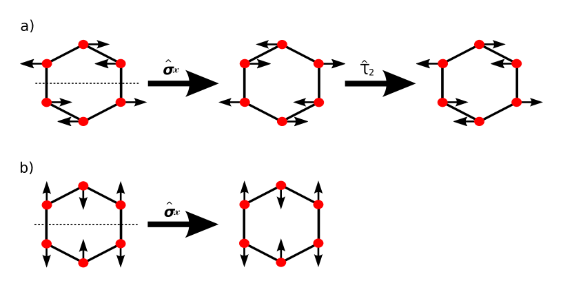
Figure 4: Schematic representations of the dynamical symmetries of the Floquet Hamiltonian (a) $\hat{\mathcal{D}}_{1}$ = $\hat{\sigma_{x}}\cdot\hat{\tau}_{2}$ (b) $\hat{\mathcal{D}}_{2}$ = $\hat{\sigma_{x}}$. The arrows show the displacements of the atom for a particular phonon mode.

The selection rules for the sidebands and its polarisation directions are obtained from the DSs as shown in Fig. 4 and requires a condition as $\hat{\mathcal{D}}\mathcal{R}_{m}(t)=\mathcal{R}_{m}(t)$. We assume that the temporal part of the $m^{\rm th}$-order sideband as $e^{i(\omega_{0}\pm m\omega_{\textrm{ph}})t+\phi_{0}}$, and of the probe laser pulse as $e^{i\omega_{0}t}$. In such situation, the Raman tensor is explicitly written as

$$\mathcal{R}_{m}(t)=e^{i(\pm m\omega_{\textrm{ph}}t+\phi_{0})}\begin{bmatrix}E_{s,m_{x}}E^{*}_{x}&E_{s,m_{x}}E^{*}_{y}\\ E_{s,m_{y}}E^{*}_{x}&E_{s,m_{y}}E^{*}_{y}\end{bmatrix}.$$ (9)

When the probe laser is polarised along X-axis, the invariance condition for the Raman tensor $\hat{\mathcal{D}_{1}}\mathcal{R}_{m}(t)=\mathcal{R}_{m}(t)$ reduces to

$$e^{i(\pm m\omega_{\textrm{ph}}t)}\begin{bmatrix}E_{s,m_{x}}\\ E_{s,m_{y}}\end{bmatrix}=e^{i[\pm m(\omega_{\textrm{ph}}t+\pi)]}\begin{bmatrix}E_{s,m_{x}}\\ -E_{s,m_{y}}\end{bmatrix}.$$ (10)

The selection rule for the $m^{\rm th}$-order sideband is as follows: when $m$ is odd (even), the polarisation of the sideband will be along the Y(X) direction. Our observations in Fig. 2(a) are consistent with Eq. (10).

When the iLO phonon mode is excited and the probe pulse is along $\mathsf{\Gamma-M}$ direction, $\hat{\sigma}_{y}\cdot\tau_{2}$, and $\hat{C}_{2Z}$ are the DSs, which leave the Raman tensor invariant. It is straightforward to see that the selection rules for the $m^{\rm th}$-order sideband are deduced as: when $m$ is odd (even), the polarisation of the sidebands will be along the X(Y) direction. On the other hand, when the iTO phonon mode is excited and the probe pulse is along $\mathsf{\Gamma-K}$ ($\mathsf{\Gamma-M}$) direction, $\hat{\sigma}_{x}$ ($\hat{\sigma}_{y}$) is the DS, which yields Raman tensor invariant [see Fig. 4(b)]. This symmetry restricts the polarisation of the sidebands to be along the direction of the probe pulse. Our results are consistent with the observation made in Fig. 2. With the increased intensity of the probe, higher-order harmonics and sidebands will appear.

To summarise, we have established that high-harmonic spectroscopy is responsive to the coherent lattice dynamics in solids. The high-harmonic spectrum is modulated by the frequency of the excited phonon mode within the solid. Both in-plane E_2g Raman-active phonon modes of the monolayer graphene lead to the generation of higher-order sidebands, along with the main harmonic peaks. In the case of iLO phonon mode excitation, the even- and odd-order sidebands are polarised parallel and perpendicular to the polarisation of probe harmonic pulse, respectively. In the case of iTO phonon mode, all sidebands are polarised along the probe harmonic pulse’s polarisation. The polarisations of the sidebands are dictated by the dynamical symmetries of the combined system, which includes the phonon modes and probe laser pulse. Therefore, the polarisation properties are a sensitive probe of these dynamical symmetries. The presence of high-harmonic signal perpendicular to the polarisation of the probe pulse is a signature of lattice excitation-driven symmetry breaking of the reflection plane. The present work is paving a way for probing phonon-driven processes in solids and non-linear phononics with sub-cycle temporal resolution.

References

- Ferray et al. (1988) M. Ferray, A. L’Huillier, X. F. Li, L. A. Lompre, G. Mainfray, and C. Manus, Journal of Physics B 21, L31 (1988).
- Ghimire et al. (2011) S. Ghimire, A. D. DiChiara, E. Sistrunk, P. Agostini, L. F. DiMauro, and D. A. Reis, Nature Physics 7, 138 (2011).
- Vampa et al. (2015) G. Vampa, T. J. Hammond, N. Thiré, B. E. Schmidt, F. Légaré, C. R. McDonald, T. Brabec, D. D. Klug, and P. B. Corkum, Physical Review Letters 115, 193603 (2015).
- Luu et al. (2015) T. T. Luu, M. Garg, S. Y. Kruchinin, A. Moulet, M. T. Hassan, and E. Goulielmakis, Nature 521, 498 (2015).
- Lanin et al. (2017) A. A. Lanin, E. A. Stepanov, A. B. Fedotov, and A. M. Zheltikov, Optica 4, 516 (2017).
- Mrudul et al. (2019) M. S. Mrudul, A. Pattanayak, M. Ivanov, and G. Dixit, Physical Review A 100, 043420 (2019).
- Tancogne-Dejean et al. (2017) N. Tancogne-Dejean, O. D. Mücke, F. X. Kärtner, and A. Rubio, Physical review letters 118, 087403 (2017).
- Mrudul et al. (2020) M. S. Mrudul, N. Tancogne-Dejean, A. Rubio, and G. Dixit, npj Computational Materials 6, 1 (2020).
- Pattanayak et al. (2020) A. Pattanayak, M. S. Mrudul, and G. Dixit, Physical Review A 101, 013404 (2020).
- Mrudul et al. (2021) M. Mrudul, Á. Jiménez-Galán, M. Ivanov, and G. Dixit, Optica 8, 422 (2021).
- Jiménez-Galán et al. (2020) Á. Jiménez-Galán, R. Silva, O. Smirnova, and M. Ivanov, Nature Photonics 14, 728 (2020).
- Langer et al. (2018) F. Langer, C. P. Schmid, S. Schlauderer, M. Gmitra, J. Fabian, P. Nagler, C. Schüller, T. Korn, P. Hawkins, J. Steiner, et al., Nature 557, 76 (2018).
- Mrudul and Dixit (2021a) M. Mrudul and G. Dixit, Journal of Physics B 54, 224001 (2021a).
- Schubert et al. (2014) O. Schubert, M. Hohenleutner, F. Langer, B. Urbanek, C. Lange, U. Huttner, D. Golde, T. Meier, M. Kira, S. W. Koch, and R. Huber, Nature Photonics 8, 119 (2014).
- Bauer and Hansen (2018) D. Bauer and K. K. Hansen, Physical Review Letters 120, 177401 (2018).
- Silva et al. (2018) R. E. F. Silva, I. V. Blinov, A. N. Rubtsov, O. Smirnova, and M. Ivanov, Nature Photonics 12, 266 (2018).
- Bai et al. (2020) Y. Bai, F. Fei, S. Wang, N. Li, X. Li, F. Song, R. Li, Z. Xu, and P. Liu, Nature Physics , 1 (2020).
- Imai et al. (2020) S. Imai, A. Ono, and S. Ishihara, Physical Review Letters 124, 157404 (2020).
- Borsch et al. (2020) M. Borsch, C. P. Schmid, L. Weigl, S. Schlauderer, N. Hofmann, C. Lange, J. T. Steiner, S. W. Koch, R. Huber, and M. Kira, Science 370, 1204 (2020).
- Baykusheva et al. (2021) D. Baykusheva, A. Chacón, J. Lu, T. P. Bailey, J. A. Sobota, H. Soifer, P. S. Kirchmann, C. Rotundu, C. Uher, T. F. Heinz, et al., Nano Letters 21, 8970 (2021).
- Bharti et al. (2022) A. Bharti, M. Mrudul, and G. Dixit, Physical Review B 105, 155140 (2022).
- Pattanayak et al. (2022) A. Pattanayak, S. Pujari, and G. Dixit, Scientific Reports 12, 1 (2022).
- Chacón et al. (2020) A. Chacón, D. Kim, W. Zhu, S. P. Kelly, A. Dauphin, E. Pisanty, A. S. Maxwell, A. Picón, M. F. Ciappina, D. E. Kim, et al., Physical Review B 102, 134115 (2020).
- Shao et al. (2022) C. Shao, H. Lu, X. Zhang, C. Yu, T. Tohyama, and R. Lu, Physical Review Letters 128, 047401 (2022).
- Lakhotia et al. (2020) H. Lakhotia, H. Y. Kim, M. Zhan, S. Hu, S. Meng, and E. Goulielmakis, Nature 583, 55 (2020).
- Mankowsky et al. (2016) R. Mankowsky, M. Först, and A. Cavalleri, Reports on Progress in Physics 79, 064503 (2016).
- Hollinger et al. (2019) R. Hollinger, V. Shumakova, A. Pugžlys, A. Baltuška, S. Khujanov, C. Spielmann, and D. Kartashov, in EPJ Web of Conferences, Vol. 205 (EDP Sciences, 2019) p. 02025.
- Patchkovskii (2009) S. Patchkovskii, Physical Review Letters 102, 253602 (2009).
- Wagner et al. (2006) N. L. Wagner, A. Wüest, I. P. Christov, T. Popmintchev, X. Zhou, M. M. Murnane, and H. C. Kapteyn, Proceedings of the National Academy of Sciences 103, 13279 (2006).
- Le et al. (2012) A.-T. Le, T. Morishita, R. Lucchese, and C. D. Lin, Physical Review Letters 109, 203004 (2012).
- Baker et al. (2006) S. Baker, J. S. Robinson, C. Haworth, H. Teng, R. Smith, C. C. Chirila?, M. Lein, J. Tisch, and J. P. Marangos, Science 312, 424 (2006).
- Lein (2005) M. Lein, Physical review letters 94, 053004 (2005).
- Wörner et al. (2011) H. J. Wörner, J. B. Bertrand, B. Fabre, J. Higuet, H. Ruf, A. Dubrouil, S. Patchkovskii, M. Spanner, Y. Mairesse, V. Blanchet, et al., Science 334, 208 (2011).
- Niedziela et al. (2019) J. Niedziela, D. Bansal, A. May, J. Ding, T.L.-Atkins, G. Ehlers, D. Abernathy, A. Said, and O. Delaire, Nature Physics 15, 73 (2019).
- Dove (1993) M. Dove, Introduction to Lattice Dynamics (Cambridge University Press, Cambridge, 1993).
- Katsuki et al. (2013) H. Katsuki, J. Delagnes, K. Hosaka, K. Ishioka, H. Chiba, E. Zijlstra, M. Garcia, H. Takahashi, K. Watanabe, M. Kitajima, et al., Nature communications 4, 1 (2013).
- Bansal et al. (2020) D. Bansal, J. L. Niedziela, S. Calder, T. Lanigan-Atkins, R. Rawl, A. H. Said, D. L. Abernathy, A. I. Kolesnikov, H. Zhou, and O. Delaire, Nature Physics 16, 669 (2020).
- Hase et al. (2015) M. Hase, P. Fons, K. Mitrofanov, A. V. Kolobov, and J. Tominaga, Nature communications 6, 1 (2015).
- Bansal et al. (2018) D. Bansal, J. Niedziela, R. Sinclair, V. Garlea, D. Abernathy, S. Chi, Y. Ren, H. Zhou, and O. Delaire, Nature Communications 9, 15 (2018).
- Fultz (2010) B. Fultz, Progress in Materials Science 55, 247 (2010).
- Gambetta et al. (2006) A. Gambetta, C. Manzoni, E. Menna, M. Meneghetti, G. Cerullo, G. Lanzani, S. Tretiak, A. Piryatinski, A. Saxena, R. Martin, et al., Nature Physics 2, 515 (2006).
- Dhar et al. (1994) L. Dhar, J. A. Rogers, and K. A. Nelson, Chemical Reviews 94, 157 (1994).
- Debnath et al. (2021) T. Debnath, D. Sarker, H. Huang, Z.-K. Han, A. Dey, L. Polavarapu, S. V. Levchenko, and J. Feldmann, Nature communications 12, 1 (2021).
- Graf et al. (2007) D. Graf, F. Molitor, K. Ensslin, C. Stampfer, A. Jungen, C. Hierold, and L. Wirtz, Nano Letters 7, 238 (2007).
- Virga et al. (2019) A. Virga, C. Ferrante, G. Batignani, D. De Fazio, A. Nunn, A. Ferrari, G. Cerullo, and T. Scopigno, Nature Communications 10, 1 (2019).
- Koivistoinen et al. (2017) J. Koivistoinen, P. Myllyperkio, and M. Pettersson, Journal of Physical Chemistry Letters 8, 4108 (2017).
- Rana et al. (2021) N. Rana, A. P. Roy, D. Bansal, and G. Dixit, npj Computational Materials 7, 1 (2021).
- Brown et al. (2019) S. B. Brown, A. Gleason, E. Galtier, A. Higginbotham, B. Arnold, A. Fry, E. Granados, A. Hashim, C. G. Schroer, A. Schropp, et al., Science advances 5, eaau8044 (2019).
- Flannigan (2018) D. J. Flannigan, Physics 11, 53 (2018).
- Gierz et al. (2015) I. Gierz, M. Mitrano, H. Bromberger, C. Cacho, R. Chapman, E. Springate, S. Link, U. Starke, B. Sachs, M. Eckstein, et al., Physical Review Letters 114, 125503 (2015).
- Moulet et al. (2017) A. Moulet, J. B. Bertrand, T. Klostermann, A. Guggenmos, N. Karpowicz, and E. Goulielmakis, Science 357, 1134 (2017).
- Géneaux et al. (2020) R. Géneaux, C. J. Kaplan, L. Yue, A. D. Ross, J. E. Bækhøj, P. M. Kraus, H.-T. Chang, A. Guggenmos, M.-Y. Huang, M. Zürch, et al., Physical Review Letters 124, 207401 (2020).
- Kim et al. (2013) J.-H. Kim, A. Nugraha, L. Booshehri, E. Hároz, K. Sato, G. Sanders, K.-J. Yee, Y.-S. Lim, C. Stanton, R. Saito, et al., Chemical Physics 413, 55 (2013).
- Mohanty and Heller (2019) V. Mohanty and E. J. Heller, Proceedings of the National Academy of Sciences 116, 18316 (2019).
- Rodriguez-Vega et al. (2021) M. Rodriguez-Vega, M. Vogl, and G. A. Fiete, Physical Review B 104, 245135 (2021).
- Wang and Fischer (2014) J. Wang and S. Fischer, Physical Review B 89, 245421 (2014).
- Moon and Koshino (2013) P. Moon and M. Koshino, Physical Review B 87, 205404 (2013).
- Currie et al. (2011) M. Currie, J. D. Caldwell, F. J. Bezares, J. Robinson, T. Anderson, H. Chun, and M. Tadjer, Applied Physics Letters 99, 211909 (2011).
- Heide et al. (2018) C. Heide, T. Higuchi, H. B. Weber, and P. Hommelhoff, Physical Review Letters 121, 207401 (2018).
- Higuchi et al. (2017) T. Higuchi, C. Heide, K. Ullmann, H. B. Weber, and P. Hommelhoff, Nature 550, 224 (2017).
- Yoshikawa et al. (2017) N. Yoshikawa, T. Tamaya, and K. Tanaka, Science 356, 736 (2017).
- Mrudul and Dixit (2021b) M. Mrudul and G. Dixit, Physical Review B 103, 094308 (2021b).
- Al-Naib et al. (2014) I. Al-Naib, J. E. Sipe, and M. M. Dignam, Physical Review B 90, 245423 (2014).
- Du et al. (2021) M. Du, C. Liu, Z. Zeng, and R. Li, Physical Review A 104, 033113 (2021).
- Neufeld et al. (2019) O. Neufeld, D. Podolsky, and O. Cohen, Nature communications 10, 1 (2019).
- Nagai et al. (2020) K. Nagai, K. Uchida, N. Yoshikawa, T. Endo, Y. Miyata, and K. Tanaka, Communications Physics 3, 1 (2020).