Communication Lower Bounds and Optimal Algorithms for Multiple Tensor-Times-Matrix Computation

Abstract

Multiple Tensor-Times-Matrix (Multi-TTM) is a key computation in algorithms for computing and operating with the Tucker tensor decomposition, which is frequently used in multidimensional data analysis. We establish communication lower bounds that determine how much data movement is required to perform the Multi-TTM computation in parallel. The crux of the proof relies on analytically solving a constrained, nonlinear optimization problem. We also present a parallel algorithm to perform this computation that organizes the processors into a logical grid with twice as many modes as the input tensor. We show that with correct choices of grid dimensions, the communication cost of the algorithm attains the lower bounds and is therefore communication optimal. Finally, we show that our algorithm can significantly reduce communication compared to the straightforward approach of expressing the computation as a sequence of tensor-times-matrix operations.

15A69, 68Q17, 68Q25, 68W10, 68W15, 68W40

1 Introduction

The Tucker tensor decomposition is a low-rank representation or approximation that enables significant compression of multidimensional data. The Tucker format consists of a core tensor, which is much smaller than the original data tensor, along with a factor matrix for each mode, or dimension, of the data. Computations involving Tucker-format tensors, such as tensor inner products, often require far fewer operations than with their full-format, dense representations. As a result, the Tucker decomposition is often used as a dimensionality reduction technique before other types of analysis are done, including computing a CP decomposition [9], for example.

A 3-way Tucker-format tensor can be expressed using the tensor notation $\bm{\mathscr{{T}}}=\bm{\mathscr{{G}}}\times_{1}{\bm{\mathbf{{A}}}}^{(1)}\times_{2}{\bm{\mathbf{{A}}}}^{(2)}\times_{3}{\bm{\mathbf{{A}}}}^{(3)}$, where $\bm{\mathscr{{G}}}$ is the 3-way core tensor, ${\bm{\mathbf{{A}}}}^{(n)}$ is a tall-skinny factor matrix corresponding to mode $n$, and $\times_{n}$ denotes the tensor-times-matrix (TTM) operation in the $n$th mode [18]. Here, $\bm{\mathscr{{T}}}$ is the full-format representation of the tensor that can be constructed explicitly by performing multiple TTM operations. We call this collective operation the Multi-TTM computation, which is the focus of this work.

Multi-TTM is a fundamental computation in the context of Tucker-format tensors. When the Tucker decomposition is used as a data compression tool, Multi-TTM is exactly the decompression operation, which is necessary when the full format is required for visualization [19], for example. In the case of full decompression, the input tensor is small and the output tensor is large. One of the quasi-optimal algorithms for computing the Tucker decomposition is the Truncated Higher-Order SVD algorithm [28, 20], in which each factor matrix is computed as the leading left singular vectors of a matrix unfolding of the tensor. In this algorithm, the smaller core tensor is computed via Multi-TTM involving the larger data tensor and the computed factor matrices. When the computational costs of the matrix SVDs are reduced using randomization, Multi-TTM becomes the overwhelming bottleneck computation [23, 26].

Since the overall size of multidimensional data grows quickly, there have been many recent efforts to parallelize the computation of the Tucker decomposition and the operations on Tucker-format tensors [3, 10, 22, 12, 5]. There has also been recent progress in establishing lower bounds on the communication costs of parallel algorithms for tensor computations, including the Matricized-Tensor Times Khatri-Rao product (MTTKRP) [6, 7, 29] and symmetric tensor contractions [25]. However, to our knowledge, no communication lower bounds have been previously established for computations relating to Tucker-format tensors. In this work, we prove communication lower bounds for a class of Multi-TTM algorithms. Additionally, we provide a parallel algorithm that attains the lower bound to within a constant factor and is therefore communication optimal.

To minimize the number of arithmetic operations in a Multi-TTM computation, the TTM operations should be performed in sequence, forming temporary intermediate tensors after each step. A single TTM corresponds to a matrix multiplication along a particular mode of the tensor, therefore a series of matrix multiplications is performed in the sequence approach to compute the final result. One of the key observations of this work is that when Multi-TTM is performed in parallel, this approach may communicate more data than necessary, even if communication-optimal algorithms are used for each individual TTM. By considering the Multi-TTM computation as a whole, we can devise atomic parallel algorithms that can communicate less than this TTM-in-Sequence approach, often with negligible increase in computation. Our proposed algorithm provides greatest benefit when the input and output tensors vary greatly in size.

The main contributions of this paper are to

• establish communication lower bounds for the parallel atomic Multi-TTM computation;

• propose a communication optimal parallel algorithm;

• show that in many typical scenarios, the straightforward approach based on a sequence of TTM operations communicates more than performing Multi-TTM as a whole.

The rest of the paper is organized as follows. Section 2 describes previous work on communication lower bounds for matrix multiplication and some tensor operations. In Section 3, we present our notations and preliminaries for the general Multi-TTM computation. To reduce the complexity of notations, we first focus on $3$-dimensional Multi-TTM computation for which we present communication lower bounds and a communication optimal algorithm in Section 4 and Section 5, respectively. In Section 6, we validate the optimality of the proposed algorithm and show that it significantly reduces communication compared to the TTM-in-Sequence approach with negligible increase in computation in many practical cases. We present our general results in Sections 7 and 8, and propose conclusions and perspectives in Section 9.

2 Related Work

A number of studies have focused on communication lower bounds for matrix multiplication, starting with the work by Hong and Kung [15] to determine the minimum number of I/O operations for sequential matrix multiplication using the red-blue pebble game. Irony et al. [16] extended this work for the parallel case. Demmel et al. [14] studied memory independent communication lower bounds for rectangular matrix multiplication based on aspect ratios of matrices. Recently, Smith et al. [24] and Al Daas et al. [1] have tightened communication lower bounds for matrix multiplication. Ballard et al. [4] extended communication lower bounds of the matrix multiplication for any computations that can be written as $3$ nested loops. Christ et al. [13] generalized the method to prove communication lower bounds of $3$ nested loop computations for arbitrary loop nesting. We apply their approach to our Multi-TTM definition.

There is limited work on communication lower bounds for tensor operations. Solomonik et al. [25] proposed communication lower bounds for symmetric tensor contraction algorithms. Ballard et al. [6] proposed communication lower bounds for MTTKRP computation with cubical tensors. This work is extended in [7] to handle varying tensor dimensions. A sequential lower bound for tile-based MTTKRP algorithms is proved by Ziogas et al. [29]. We use some results from [6, 7] to prove communication lower bounds for Multi-TTM.

3 Notations and Preliminaries

In this section, we present our notations and basic lemmas for $d$-dimensional Multi-TTM computation. In Sections 4, 5 and 6, we focus on $d=3$, i.e., $\bm{\mathscr{{Y}}}$ = $\bm{\mathscr{{X}}}\times_{1}{{\bm{\mathbf{{A}}}}^{(1)}}^{\sf T}\times_{2}{{\bm{\mathbf{{A}}}}^{(2)}}^{\sf T}\times_{3}{{\bm{\mathbf{{A}}}}^{(3)}}^{\sf T}$. We present our general results in Sections 7 and 8.

We use boldface uppercase Euler script letters to denote tensors ($\bm{\mathscr{{X}}}$) and boldface uppercase letters with superscripts to denote matrices (${\bm{\mathbf{{A}}}}^{(1)}$). We use lowercase letters with subscripts to denote sizes ($n_{1}$) and add the prime symbol to them to denote the indices ($n_{1}^{\prime}$). We use one-based indexing throughout and $[d]$ to denote the set $\{1,2,\cdots,d\}$. To improve the presentation, we denote the product of elements having the same lowercase letter with all subscripts by the lowercase letter only ($n_{1}\cdots n_{d}$ by $n$ and $r_{1}\cdots r_{d}$ by $r$). We denote the product of the $i$ rightmost terms with the capital letter with subscript $i$, $N_{i}=\prod_{j=d-i+1}^{d}n_{j}$ and $R_{i}=\prod_{j=d-i+1}^{d}r_{i}$, thus $n=N_{d}$, and $n_{d}=N_{1}$.

Let $\bm{\mathscr{{Y}}}\in\mathbb{R}^{r_{1}\times\cdots\times r_{d}}$ be the $d$-mode output tensor, $\bm{\mathscr{{X}}}\in\mathbb{R}^{n_{1}\times\cdots\times n_{d}}$ be the $d$-mode input tensor, and ${\bm{\mathbf{{A}}}}^{(k)}\in\mathbb{R}^{n_{k}\times r_{k}}$ be the matrix of the $k$th mode. Then the Multi-TTM computation can be represented as $\bm{\mathscr{{Y}}}=\bm{\mathscr{{X}}}\times_{1}{{\bm{\mathbf{{A}}}}^{(1)}}^{\sf T}\cdots\times_{d}{{\bm{\mathbf{{A}}}}^{(d)}}^{\sf T}$. Without loss of generality and to simplify notation, we consider that the input tensor $\bm{\mathscr{{X}}}$ is larger than the output tensor $\bm{\mathscr{{Y}}}$, or $n\geq r$. This corresponds to computing the core tensor of a Tucker decomposition given computed factor matrices, for example. However, the opposite relationship where the output tensor is larger (e.g., $\bm{\mathscr{{X}}}=\bm{\mathscr{{Y}}}\times_{1}{{\bm{\mathbf{{A}}}}^{(1)}}\cdots\times_{d}{{\bm{\mathbf{{A}}}}^{(d)}}$) is also an important use case, corresponding to forming an explicit representation of a (sub-)tensor of a Tucker-format tensor. Our results extend straightforwardly to this case. We consider $d$-dimensional input and output tensors and therefore assume $n_{i}\geq 2$ and $r_{i}\geq 2$ for $1\leq i\leq d$. We also assume without loss of generality that the tensor modes are ordered in such a way that $n_{1}r_{1}\leq n_{2}r_{2}\leq\cdots\leq n_{d}r_{d}$.

Definition 3.1.

Let $\bm{\mathscr{{X}}}$ be an $n_{1}\times\cdots\times n_{d}$ tensor, $\bm{\mathscr{{Y}}}$ be an $r_{1}\times\cdots\times r_{d}$ tensor, and ${\bm{\mathbf{{A}}}}^{(j)}$ be an $n_{j}\times r_{j}$ matrix for $j\in[d]$. Multi-TTM computes

$$\bm{\mathscr{{Y}}}=\bm{\mathscr{{X}}}\times_{1}{{\bm{\mathbf{{A}}}}^{(1)}}^{\sf T}\cdots\times_{d}{{\bm{\mathbf{{A}}}}^{(d)}}^{\sf T}$$

where for each $(r_{1}^{\prime},\ldots,r_{d}^{\prime})\in[r_{1}]\times\cdots\times[r_{d}]$,

(1) $$\bm{\mathscr{{Y}}}(r_{1}^{\prime},\ldots,r_{d}^{\prime})=\sum_{\{n_{k}^{\prime}\in[n_{k}]\}_{k\in[d]}}\bm{\mathscr{{X}}}(n_{1}^{\prime},\ldots,n_{d}^{\prime})\prod_{j\in[d]}{\bm{\mathbf{{A}}}}^{(j)}(n_{j}^{\prime},r_{j}^{\prime}).$$

Let us consider an example when $d=2$. In this scenario, the input and output tensors are in fact matrices ${\bm{\mathbf{{X}}}},{\bm{\mathbf{{Y}}}}$, and ${\bm{\mathbf{{Y}}}}={\bm{\mathbf{{A}}}}^{(1){\sf T}}{\bm{\mathbf{{X}}}}{\bm{\mathbf{{A}}}}^{(2)}$. As mentioned earlier, Multi-TTM computation can be performed as a sequence of TTM operations, in this case two matrix multiplications. However, we define the Multi-TTM to perform all the products at once for each term of the summation of equation 1. Our definition comes at greater arithmetic cost, as partial $(d+1)$-ary multiplies are not computed and reused, but we will see that this approach can reduce communication cost. We describe how the extra computation can often be reduced to a negligible cost in Subsection 5.1 and compare it to the computation cost of TTM-in-Sequence in Subsection 6.2.2.

We can write pseudocode for the Multi-TTM with the following:

for $$n_{1}^{\prime}=1{:}n_{1} n_{d}^{\prime}=1{:}n_{d}$$, …, for ,

for $$r_{1}^{\prime}=1{:}r_{1} r_{d}^{\prime}=1{:}r_{d}$$, …, for ,

$$\quad\quad\bm{\mathscr{{Y}}}(r_{1}^{\prime},\ldots,r_{d}^{\prime})\ +=\bm{\mathscr{{X}}}(n_{1}^{\prime},\ldots,n_{d}^{\prime})\,\cdot{\bm{\mathbf{{A}}}}^{(1)}(n_{1}^{\prime},r_{1}^{\prime})\cdot\cdots\cdot{\bm{\mathbf{{A}}}}^{(N)}(n_{d}^{\prime},r_{d}^{\prime})$$

Definition 3.2.

A parallel atomic Multi-TTM algorithm computes each term of the summation of equation 1 atomically on a unique processor, but it can distribute the $nr$ terms over processors in any way.

Here atomic computation of a single $(d{+}1)$-ary multiplication for a parallel algorithm means that all the multiplications of this operation are performed on only one processor, i.e., all $d+1$ inputs are accessed on that processor in order to compute the single output value. This assumption is necessary for our communication lower bounds. Processors can reorganize their local atomic operations to reduce computational costs without changing the communication or violating parallel atomicity. However it is reasonable for an algorithm to break this assumption in order to improve arithmetic costs by reusing partial results across processors, and we compare against such algorithms in Section 6.

3.1 Parallel Computation Model

We consider that the computation is distributed across $P$ processors. Each processor has its own local memory and is connected to all other processors via a fully connected network. Every processor can operate on data in its local memory and must communicate to access data of other processors. Hence, communication refers to send and receive operations that transfer data from local memory to the network and vice-versa. Communication cost mainly depends on two factors – the amount of data communicated (bandwidth cost) and the number of messages (latency cost). Latency cost is dominated by bandwidth cost for computations involving large messages, so we focus on bandwidth cost in this work and refer it as communication cost throughout the text. We assume the links of the network are bidirectional and that the communication cost is independent of the number of pairs of processors that are communicating. Each processor can send and receive at most one message at the same time. In our model, the communication cost of an algorithm refers to the cost along the critical path.

3.2 Existing Results

Our work relies on two fundamental results. The first, a geometric result on lattices, allows us to relate the volume of computation to the amount of data accessed by determining the maximum data reuse. The result is a specialization of the Hölder-Brascamp-Lieb inequalities [8]. This result has previously been used to derive lower bounds for tensor computations [6, 7, 13, 17] in a similar way to the use of the Loomis-Whitney inequality [21] in derivations of communication lower bounds for several linear algebra computations [4]. The result is proved in [13], but we use the statement from [6, Lemma 4.1]. Here ${\bm{\mathbf{{1}}}}$ represents a vector of all ones and $\geq$ relation between vectors applies elementwise.

Lemma 3.3.

Consider any positive integers $\ell$ and $m$ and any $m$ projections $\phi_{j}:\mathbb{Z}^{\ell}\rightarrow\mathbb{Z}^{\ell_{j}}$ ($\ell_{j}\leq\ell$), each of which extracts $\ell_{j}$ coordinates $S_{j}\subseteq[\ell]$ and forgets the $\ell-\ell_{j}$ others. Define $\mathcal{C}=\big{\{}{\bm{\mathbf{{s}}}}={[s_{1}\ \cdots\ s_{m}]^{\sf T}:0\leq s_{i}\leq 1\text{ for }i=1,2,\cdots,m\text{ and }}{\bm{\mathbf{{\Delta}}}}\cdot{\bm{\mathbf{{s}}}}\geq{\bm{\mathbf{{1}}}}\big{\}}\text{,}$ where the $\ell\times m$ matrix ${\bm{\mathbf{{\Delta}}}}$ has entries ${\bm{\mathbf{{\Delta}}}}_{i,j}=1\text{ if }i\in S_{j}\text{ and }{\bm{\mathbf{{\Delta}}}}_{i,j}=0\text{ otherwise}\text{.}$ If $[s_{1}\ \cdots\ s_{m}]^{\sf T}\in\mathcal{C}$, then for all $F\subseteq\mathbb{Z}^{\ell}$,

$$|F|\leq\prod_{j\in[m]}|\phi_{j}(F)|^{s_{j}}\text{.}$$

The second result, a general constrained optimization problem, allows us to cast the communication cost of an algorithm as the objective function in an optimization problem where the constraints are imposed by properties of the computation within the algorithm. A version of the result is proved in [7, Lemma 5.1] and used to derive the general communication lower bound for MTTKRP.

Theorem 3.4.

Consider the constrained optimization problem:

$$\min\sum_{j\in[d]}x_{j}$$

such that

$$\frac{nr}{P}\leq\prod_{j\in[d]}x_{j}\quad\text{and}\quad 0\leq x_{j}\leq k_{j}\quad\text{for all}\quad 1\leq j\leq d$$

for some positive constants $k_{1}\leq k_{2}\leq\cdots\leq k_{d}$ with $\prod_{j\in[d]}k_{j}=nr$. Then the minimum value of the objective function is

$$I\left(K_{I}/P\right)^{1/I}+\sum_{j\in[d-I]}k_{j}$$

where we use the notation $K_{I}=\prod_{j=d-I+1}^{d}k_{j}$ and $1\leq I\leq d$ is defined such that $L_{I}\leq P<L_{I+1}$.

$$\text{Here}\quad L_{j}=\frac{K_{j}}{(k_{d-j+1})^{j}}\quad\text{for}\quad 1\leq j\leq d\quad\text{and}\quad L_{d+1}=\infty.\qquad\qquad\qquad$$

The minimum is achieved at the point ${\bm{\mathbf{{x}}}}^{*}$ defined by ${x_{j}}^{*}=k_{j}$ for $1\leq j\leq d-I$, ${x_{\ell}}^{*}=\left(K_{I}/P\right)^{1/I}$ for $d-I<\ell\leq d$.

While Theorem 3.4 can be straightforwardly derived from the previous work, we provide an alternate proof in Appendix A. We represent it in this form to be directly applicable to all the constrained optimization problems in this paper. The constraints $nr/P\leq\prod_{j\in[d]}x_{j}$ and $\prod_{j\in[d]}k_{j}=nr$ are derived from the Multi-TTM computation. The equality constraint on $\prod_{j\in[d]}k_{j}$ implies that there is always a feasible solution to the optimization problem for $P\geq 1$. We calculate the ranges of $P$ for each $I$ in Corollaries 4.1, 4.2 and 7.1.

4 Lower Bounds for $3$-dimensional Multi-TTM

We obtain the lower bound results for 3D tensors in this section, presented as Theorem 4.3. The lower bound is independent of the size of the local memory of each processor, similar to previous results for matrix multiplication [1, 14] and MTTKRP [6, 7], and it varies with respect to the number of processors $P$ relative to the matrix and tensor dimensions of the problem.

The proof focuses on a processor that performs $1/P$th of the computation and owns at most $1/P$th of the data. It reduces the problem of finding a lower bound on the amount of data the processor must communicate to solving a constrained optimization problem: we seek to minimize the number of elements of the matrices and tensors that the processor must access or partially compute in order to execute its computation subject to structure constraints of Multi-TTM. The most important constraint derives from Lemma 3.3, which relates a subset of the computation within a Multi-TTM algorithm to the data it requires. The other constraints provide upper bounds on the data required from each array. The upper bounds are necessary to establish the tightest lower bounds in the cases where $P$ is small. We show that the optimization problem can be separated into two independent problems, one for the matrix data and one for the tensor data. Corollaries 4.1 and 4.2 state the two constrained optimization problems along with their analytic solutions, both of which follow from Theorem 3.4. That is, setting $d=3$, $k_{1}=n_{1}r_{1}$, $k_{2}=n_{2}r_{2}$ and $k_{3}=n_{3}r_{3}$ in Theorem 3.4, we obtain Corollary 4.1. Similarly, setting $d=2$ with $k_{1}=r$ and $k_{2}=n$, we obtain Corollary 4.2. We recall here that $r=r_{1}r_{2}r_{3}$ and $n=n_{1}n_{2}n_{3}$.

Corollary 4.1.

Consider the following optimization problem:

$$\min_{x,y,z}x+y+z$$

such that

$$\frac{nr}{P} \leq xyz$$

$$0 \leq\phantom{y}x\phantom{z}\leq n_{1}r_{1}$$

$$0 \leq\phantom{x}y\phantom{z}\leq n_{2}r_{2}$$

$$0 \leq\phantom{x}z\phantom{y}\leq n_{3}r_{3},$$

where $n_{1}r_{1}\leq n_{2}r_{2}\leq n_{3}r_{3}$, and $n_{1},n_{2},n_{3},r_{1},r_{2},r_{3},P\geq 1$. The optimal solution $({x}^{*},{y}^{*},{z}^{*})$ depends on the relative values of the constraints, yielding three cases:

1. if $P<\frac{n_{3}r_{3}}{n_{2}r_{2}}$, then ${x}^{*}=n_{1}r_{1}$, ${y}^{*}=n_{2}r_{2}$, ${z}^{*}=\frac{n_{3}r_{3}}{P}$;

2. if $\frac{n_{3}r_{3}}{n_{2}r_{2}}\leq P<\frac{n_{2}n_{3}r_{2}r_{3}}{n_{1}^{2}r_{1}^{2}}$, then ${x}^{*}=n_{1}r_{1}$, ${y}^{*}={z}^{*}=\big{(}\frac{n_{2}n_{3}r_{2}r_{3}}{P}\big{)}^{\frac{1}{2}}$;

3. if $\frac{n_{2}n_{3}r_{2}r_{3}}{n_{1}^{2}r_{1}^{2}}\leq P$, then ${x}^{*}={y}^{*}={z}^{*}=\big{(}\frac{nr}{P}\big{)}^{\frac{1}{3}}$;

which can be visualized as follows.

Corollary 4.2.

Consider the following optimization problem:

$$\min_{u,v}u+v$$

such that

$$\frac{nr}{P} \leq uv$$

$$0 \leq\;u\;\leq r$$

$$0 \leq\;v\;\leq n,$$

where $n\geq r$, and $n,r,P\geq 1$. The optimal solution $({u}^{*},{v}^{*})$ depends on the relative values of the constraints, yielding two cases:

1. if $P<\frac{n}{r}$, then ${u}^{*}=r$, ${v}^{*}=\frac{n}{P}$;

2. if $\frac{n}{r}\leq P$, then ${u}^{*}={v}^{*}=\big{(}\frac{nr}{P}\big{)}^{\frac{1}{2}}$;

which can be visualized as follows.

4.1 Communication Lower Bounds for Multi-TTM

We now state the lower bounds for 3-dimensional Multi-TTM. After this, we also present a corollary for cubical tensors.

Theorem 4.3.

Any computationally load balanced atomic Multi-TTM algorithm that starts and ends with one copy of the data distributed across processors involving 3D tensors with dimensions $n_{1},n_{2},n_{3}$ and $r_{1},r_{2},r_{3}$ performs at least $A+B-\left(\frac{n}{P}+\frac{r}{P}+\sum_{j=1}^{3}\frac{n_{j}r_{j}}{P}\right)$ sends or receives where

$$A =\begin{cases}n_{1}r_{1}+n_{2}r_{2}+\frac{n_{3}r_{3}}{P}&\text{ if }P<\frac{n_{3}r_{3}}{n_{2}r_{2}}\\ n_{1}r_{1}+2\left(\frac{n_{2}n_{3}r_{2}r_{3}}{P}\right)^{\frac{1}{2}}&\text{ if }\frac{n_{3}r_{3}}{n_{2}r_{2}}\leq P<\frac{n_{2}n_{3}r_{2}r_{3}}{n_{1}^{2}r_{1}^{2}}\\ 3\left(\frac{nr}{P}\right)^{\frac{1}{3}}&\text{ if }\frac{n_{2}n_{3}r_{2}r_{3}}{n_{1}^{2}r_{1}^{2}}\leq P\end{cases}$$

$$B =\begin{cases}r+\frac{n}{P}&\text{ if }P<\frac{n}{r}\\ 2\left(\frac{nr}{P}\right)^{\frac{1}{2}}&\text{ if }\frac{n}{r}\leq P\text{.}\end{cases}$$

Proof 4.4.

Let $F$ be the set of loop indices associated with the $4$-ary multiplication performed by a processor. As we assumed the algorithm is computationally load balanced, $|F|=nr/P$. We define $\phi_{\bm{\mathscr{{X}}}}(F)$, $\phi_{\bm{\mathscr{{Y}}}}(F)$ and $\phi_{j}(F)$ to be the projections of $F$ onto the indices of the arrays $\bm{\mathscr{{X}}},\bm{\mathscr{{Y}}}$, and ${\bm{\mathbf{{A}}}}^{(j)}$ for $1\leq j\leq 3$ which correspond to the elements of the array that must be accessed or partially computed by the processor.

We use Lemma 3.3 to obtain a lower bound on the number of array elements that must be accessed or partially computed by the processor. The computation involves $5$ arrays (2 tensors and 3 matrices) with $6$ loop indices (see the atomic Multi-TTM definition in Section 3), hence the $6\times 5$ matrix corresponding to the projections above is given by

$${\bm{\mathbf{{\Delta}}}}=\begin{bmatrix}{\bm{\mathbf{{I}}}}_{3\times 3}&{\bm{\mathbf{{1}}}}_{3}&{\bm{\mathbf{{0}}}}_{3}\\ {\bm{\mathbf{{I}}}}_{3\times 3}&{\bm{\mathbf{{0}}}}_{3}&{\bm{\mathbf{{1}}}}_{3}\end{bmatrix}\text{.}$$

Here ${\bm{\mathbf{{1}}}}_{3}$ and ${\bm{\mathbf{{0}}}}_{3}$ represent the 3-dimensional vectors of all ones and zeros, respectively, and ${\bm{\mathbf{{I}}}}_{3\times 3}$ represents the $3\times 3$ identity matrix. We recall from Lemma 3.3 that ${\bm{\mathbf{{\Delta}}}}_{i,j}=1$ if loop index $i$ is used to access array $j$ and ${\bm{\mathbf{{\Delta}}}}_{i,j}=0$ otherwise. The first three columns of ${\bm{\mathbf{{\Delta}}}}$ correspond to matrices and the remaining two columns correspond to tensors. In this case, we have

$$\mathcal{C}=\big{\{}{\bm{\mathbf{{s}}}}={[s_{1}\ \cdots\ s_{5}]^{\sf T}:0\leq s_{i}\leq 1\text{ for }i=1,2,\cdots,5\text{ and }}{\bm{\mathbf{{\Delta}}}}\cdot{\bm{\mathbf{{s}}}}\geq{\bm{\mathbf{{1}}}}\big{\}}\text{.}$$

Recall that ${\bm{\mathbf{{1}}}}$ represents a vector of all ones. Here ${\bm{\mathbf{{\Delta}}}}$ is not full rank, therefore, we consider all vectors ${\bm{\mathbf{{v}}}}\in\mathcal{C}$ such that ${\bm{\mathbf{{\Delta}}}}\cdot{\bm{\mathbf{{v}}}}={\bm{\mathbf{{1}}}}$. Such a vector ${\bm{\mathbf{{v}}}}$ is of the form $[a\;a\;a\;1\text{-}a\;1\text{-}a]$ where $0\leq a\leq 1$. Therefore, we obtain

$$\frac{nr}{P}\leq\Big{(}\prod_{j\in[3]}|\phi_{j}(F)|\Big{)}^{a}\big{(}|\phi_{\bm{\mathscr{{X}}}}(F)||\phi_{\bm{\mathscr{{Y}}}}(F)|\big{)}^{1\text{-}a}\text{ for all }0\leq a\leq 1.$$

The above constraint is equivalent to $\frac{nr}{P}\leq\prod_{j\in[3]}|\phi_{j}(F)|$ and $\frac{nr}{P}\leq|\phi_{\bm{\mathscr{{X}}}}(F)||\phi_{\bm{\mathscr{{Y}}}}(F)|$. To see this equivalence note that the forward direction is implied by setting $a=0$ and $a=1$. For the opposite direction, taking the first of the two constraints to the power $a$ and the second to the power $1-a$ then multiplying the two terms yields the original.

Clearly a projection onto an array cannot be larger than the array itself, thus $|\phi_{\bm{\mathscr{{X}}}}(F)|\leq n$, $|\phi_{\bm{\mathscr{{Y}}}}(F)|\leq r$, and $|\phi_{j}(F)|\leq n_{j}r_{j}$ for $1\leq j\leq 3$.

As the constraints related to projections of matrices and tensors are disjoint, we solve them separately and then sum the results to get a lower bound on the set of elements that must be accessed or partially computed by the processor. We obtain a lower bound on $A$, the number of relevant elements of the matrices by using Corollary 4.1, and a lower bound on $B$, the number of relevant elements of the tensors by using Corollary 4.2. By summing both, we get the positive terms of the lower bound.

To bound the sends or receives, we consider how much data the processor could have had at the beginning or at the end of the computation. Assuming there is exactly one copy of the data at the beginning and at the end of the computation, there must exist a processor which owns at most $1/P$ of the elements of the arrays at the beginning or at the end of the computation. By employing the previous analysis, this processor must access or partially compute $A+B$ elements of the arrays, but can only own $\frac{n}{P}+\frac{r}{P}+\sum_{j\in[3]}\frac{n_{j}r_{j}}{P}$ elements of the arrays. Thus it must perform the specified amount of sends or receives.

We denote the lower bound of Theorem 4.3 by ${\sc LB}$ and use it extensively in Subsection 5.2 while analyzing the communication cost of our parallel algorithm.

We also state the result for $3$-dimensional Multi-TTM computation with cubical tensors, which is a direct application of Theorem 4.3 with $n_{1}=n_{2}=n_{3}=n^{\frac{1}{3}}$ and $r_{1}=r_{2}=r_{3}=r^{\frac{1}{3}}$.

Corollary 4.5.

Any computationally load balanced atomic Multi-TTM algorithm that starts and ends with one copy of the data distributed across processors involving 3D cubical tensors with dimensions $n^{\frac{1}{3}}\times n^{\frac{1}{3}}\times n^{\frac{1}{3}}$ and $r^{\frac{1}{3}}\times r^{\frac{1}{3}}\times r^{\frac{1}{3}}$ (with $n\geq r$) performs at least

$$3\left(\frac{nr}{P}\right)^{\frac{1}{3}}+r-\frac{3(nr)^{\frac{1}{3}}+r}{P}$$

sends or receives when $P<\frac{n}{r}$ and at least

$$3\left(\frac{nr}{P}\right)^{\frac{1}{3}}+2\left(\frac{nr}{P}\right)^{\frac{1}{2}}-\frac{n+3(nr)^{\frac{1}{3}}+r}{P}$$

send or receives when $P\geq\frac{n}{r}$.

In particular, we note that the lower bound for cubical atomic Multi-TTM algorithms is smaller than that of a TTM-in-Sequence approach for many typical scenarios in the case $P<n/r$, as we discuss further in Section 6.

5 Parallel Algorithm for $3$-dimensional Multi-TTM

We organize $P$ processors into a $6$-dimensional $p_{1}\times p_{2}\times p_{3}\times q_{1}\times q_{2}\times q_{3}$ logical processor grid. We arrange the grid dimensions such that $p_{1}$, $p_{2}$, $p_{3}$, $q_{1}$, $q_{2}$, $q_{3}$ evenly distribute $n_{1}$, $n_{2}$, $n_{3}$, $r_{1}$, $r_{2}$, $r_{3}$, respectively. A processor coordinate is represented as $(p_{1}^{\prime},p_{2}^{\prime},p_{3}^{\prime},q_{1}^{\prime},q_{2}^{\prime},q_{3}^{\prime})$, where $1\leq p_{k}^{\prime}\leq p_{k}$, $1\leq q_{k}^{\prime}\leq q_{k}$ for $k=1,2,3$. To be consistent with our notation, we denote $p_{1}p_{2}p_{3}$ and $q_{1}q_{2}q_{3}$ by $p$ and $q$.

$\bm{\mathscr{{X}}}_{p_{1}^{\prime}p_{2}^{\prime}p_{3}^{\prime}}$ denotes the subtensor of $\bm{\mathscr{{X}}}$ owned by processors $(p_{1}^{\prime},p_{2}^{\prime},$ $p_{3}^{\prime},*,*,*)$. Similarly, $\bm{\mathscr{{Y}}}_{q_{1}^{\prime}q_{2}^{\prime}q_{3}^{\prime}}$ denotes the subtensor of $\bm{\mathscr{{Y}}}$ owned by processors $(*,*,*,q_{1}^{\prime},q_{2}^{\prime},q_{3}^{\prime})$. ${\bm{\mathbf{{A}}}}^{(1)}_{p_{1}^{\prime}q_{1}^{\prime}}$, ${\bm{\mathbf{{A}}}}^{(2)}_{p_{2}^{\prime}q_{2}^{\prime}}$ and ${\bm{\mathbf{{A}}}}^{(3)}_{p_{3}^{\prime}q_{3}^{\prime}}$ denote submatrices of ${\bm{\mathbf{{A}}}}^{(1)}$, ${\bm{\mathbf{{A}}}}^{(2)}$ and ${\bm{\mathbf{{A}}}}^{(3)}$ owned by processors $(p_{1}^{\prime},*,*,q_{1}^{\prime},*,*)$, $(*,p_{2}^{\prime},*,*,q_{2}^{\prime},*)$ and $(*,*,p_{3}^{\prime},*,*,q_{3}^{\prime})$, respectively.

We impose that there is one copy of data in the system at the start and end of the computation, and every array is distributed evenly among the sets of processors whose coordinates are different for the corresponding dimensions of the variable. For example, $\bm{\mathscr{{X}}}_{111}$ = $\bm{\mathscr{{X}}}(1:\frac{n_{1}}{p_{1}},1:\frac{n_{2}}{p_{2}},1:\frac{n_{3}}{p_{3}})$ is owned by processors $(1,1,1,*,*,*)$. Similarly, ${\bm{\mathbf{{A}}}}^{(1)}_{12}$ = ${\bm{\mathbf{{A}}}}^{(1)}(1:\frac{n_{1}}{p_{1}},\frac{r_{1}}{q_{1}}+1:2\frac{r_{1}}{q_{1}})$ is owned by processors $(1,*,*,2,*,*)$. We assume that data inside these sets of processors is also evenly distributed. For example, in the beginning, processor ($1,1,1,2,1,3$) owns $\frac{1}{P}$th portion of each input variable: $\frac{p}{P}$th portion of $\bm{\mathscr{{X}}}_{111}$, $\frac{p_{1}q_{1}}{P}$th portion of ${\bm{\mathbf{{A}}}}^{(1)}_{12}$, $\frac{p_{2}q_{2}}{P}$th portion of ${\bm{\mathbf{{A}}}}^{(2)}_{11}$, and $\frac{p_{3}q_{3}}{P}$th portion of ${\bm{\mathbf{{A}}}}^{(3)}_{13}$. Figure 1 illustrates examples of our data distribution model for two of the arrays.

      

Figure 1: Subtensor $\bm{\mathscr{{X}}}_{231}$ is distributed evenly among processors $(2,3,1,*,*,*)$. Similarly, submatrix ${\bm{\mathbf{{A}}}}^{(2)}_{31}$ is distributed evenly among processors $(*,3,*,*,1,*)$.

Algorithm 1 Parallel Atomic 3-dimensional Multi-TTM

0:  $\bm{\mathscr{{X}}}$, ${\bm{\mathbf{{A}}}}^{(1)}$, ${\bm{\mathbf{{A}}}}^{(2)}$, ${\bm{\mathbf{{A}}}}^{(3)}$, $p_{1}\times p_{2}\times p_{3}\times q_{1}\times q_{2}\times q_{3}$ logical processor grid

0:  $\bm{\mathscr{{Y}}}$ such that $\bm{\mathscr{{Y}}}=\bm{\mathscr{{X}}}\times_{1}{{\bm{\mathbf{{A}}}}^{(1)}}^{\sf T}\times_{2}{{\bm{\mathbf{{A}}}}^{(2)}}^{\sf T}\times_{3}{{\bm{\mathbf{{A}}}}^{(3)}}^{\sf T}$

1:  $(p_{1}^{\prime},p_{2}^{\prime},p_{3}^{\prime},q_{1}^{\prime},q_{2}^{\prime},q_{3}^{\prime})$ is my processor id

2:  //All-gather input tensor $\bm{\mathscr{{X}}}$

3:  $\bm{\mathscr{{X}}}_{p_{1}^{\prime}p_{2}^{\prime}p_{3}^{\prime}}$ = All-Gather($\bm{\mathscr{{X}}}$, $(p_{1}^{\prime},p_{2}^{\prime},p_{3}^{\prime},*,*,*)$)

4:  //All-gather input matrices

5:  ${\bm{\mathbf{{A}}}}^{(1)}_{p_{1}^{\prime}q_{1}^{\prime}}$ = All-Gather(${\bm{\mathbf{{A}}}}^{(1)}$, $(p_{1}^{\prime},*,*,q_{1}^{\prime},*,*)$)

6:  ${\bm{\mathbf{{A}}}}^{(2)}_{p_{2}^{\prime}q_{2}^{\prime}}$ = All-Gather(${\bm{\mathbf{{A}}}}^{(2)}$, $(*,p_{2}^{\prime},*,*,q_{2}^{\prime},*)$)

7:  ${\bm{\mathbf{{A}}}}^{(3)}_{p_{3}^{\prime}q_{3}^{\prime}}$ = All-Gather(${\bm{\mathbf{{A}}}}^{(3)}$, $(*,*,p_{3}^{\prime},*,*,q_{3}^{\prime})$)

8:  //Local computations in a temporary tensor $\bm{\mathscr{{T}}}$

9:  $\bm{\mathscr{{T}}}$ = Local-Multi-TTM($\bm{\mathscr{{X}}}_{p_{1}^{\prime}p_{2}^{\prime}p_{3}^{\prime}}$, ${\bm{\mathbf{{A}}}}^{(1)}_{p_{1}^{\prime}q_{1}^{\prime}}$, ${\bm{\mathbf{{A}}}}^{(2)}_{p_{2}^{\prime}q_{2}^{\prime}}$, ${\bm{\mathbf{{A}}}}^{(3)}_{p_{3}^{\prime}q_{3}^{\prime}}$)

10:  //Reduce-scatter the output tensor in $\bm{\mathscr{{Y}}}_{q_{1}^{\prime}q_{2}^{\prime}q_{3}^{\prime}}$

11:  Reduce-Scatter($\bm{\mathscr{{Y}}}_{q_{1}^{\prime}q_{2}^{\prime}q_{3}^{\prime}}$, $\bm{\mathscr{{T}}}$, $(*,*,*,q_{1}^{\prime},q_{2}^{\prime},q_{3}^{\prime})$)

Algorithm 1 presents a parallel algorithm to compute $3$-dimensional Multi-TTM. When it completes, $\bm{\mathscr{{Y}}}_{q_{1}^{\prime}q_{2}^{\prime}q_{3}^{\prime}}$ is distributed evenly among processors $(*,$ $*,$ $*,$ $q_{1}^{\prime},$ $q_{2}^{\prime},$ $q_{3}^{\prime})$. Figure 2 shows the steps of the algorithm for a single processor in a $3\times 3\times 3\times 3\times 3\times 3$ grid.

(a) Perform All-Gather on processors $(2,1,1,*,*,*)$ to obtain $\bm{\mathscr{{X}}}_{211}$.

(b) Perform All-Gather on processors $(2,*,*,1,*,*)$ to obtain ${\bm{\mathbf{{A}}}}^{(1)}_{21}$.

(c) Perform All-Gather on processors $(*,1,*,*,3,*)$ to obtain ${\bm{\mathbf{{A}}}}^{(2)}_{13}$.

(d) Perform All-Gather on processors $(*,*,1,*,*,1)$ to obtain ${\bm{\mathbf{{A}}}}^{(3)}_{11}$.

(e) Perform local Multi-TTM to compute partial $\bm{\mathscr{{Y}}}_{131}$.

(f) Perform Reduce-Scatter on processors $(*,*,*,1,3,1)$ to compute/distribute $\bm{\mathscr{{Y}}}_{131}$.

              

Figure 2: Steps of Alg. 1 for processor $(2,1,1,1,3,1)$, where $p_{1}=p_{2}=p_{3}=q_{1}=q_{2}=q_{3}=3$. Highlighted areas correspond to the data blocks on which the processor is operating. The dark red highlighting represents the input/output data initially/finally owned by the processor, and the light red highlighting corresponds to received/sent data from/to other processors in All-Gather/Reduce-Scatter collectives to compute $\bm{\mathscr{{Y}}}_{131}$.

5.1 Cost Analysis

Now we analyze computation and communication costs of the algorithm. The dimension of the local tensor $\bm{\mathscr{{X}}}_{p_{1}^{\prime}p_{2}^{\prime}p_{3}^{\prime}}$ is $\frac{n_{1}}{p_{1}}\times\frac{n_{2}}{p_{2}}\times\frac{n_{3}}{p_{3}}$, the dimension of the local matrix ${\bm{\mathbf{{A}}}}^{(k)}_{p_{k}^{\prime}q_{k}^{\prime}}$ is $\frac{n_{i}}{p_{i}}\times\frac{r_{i}}{q_{i}}$ for $i=1,2,3$, and the dimension of the temporary tensor $\bm{\mathscr{{T}}}$ is $\frac{r_{1}}{q_{1}}\times\frac{r_{2}}{q_{2}}\times\frac{r_{3}}{q_{3}}$. For simplicity of analysis, we assume that the numerator is divisible by the denominator for each cost expression.

The local Multi-TTM computation in Line 9 can be performed as a sequence of TTM operations to mininimize the number of arithmetic operations. Assuming the TTM operations are performed in their order, first with ${\bm{\mathbf{{A}}}}^{(1)}$, then with ${\bm{\mathbf{{A}}}}^{(2)}$, and in the end with ${\bm{\mathbf{{A}}}}^{(3)}$, then each processor performs $2\Big{(}\frac{n_{1}n_{2}n_{3}r_{1}}{p_{1}p_{2}p_{3}q_{1}}+\frac{n_{2}n_{3}r_{1}r_{2}}{p_{2}p_{3}q_{1}q_{2}}+\frac{n_{3}r_{1}r_{2}r_{3}}{p_{3}q_{1}q_{2}q_{3}}\Big{)}$ operations to perform the local computation.

Communication occurs only in the All-Gather and Reduce-Scatter collectives in Lines 3, 5, 6, 7 and 11. Each processor is involved in one All-Gather involving the input tensor, three All-Gathers involving input matrices and one Reduce-Scatter involving the output tensor. Therefore, the communication cost of the algorithm along the critical path is the sum of communication costs of these five collectives. Lines 3, 5, 6, and 7 specify $p$, $p_{1}q_{1}$, $p_{2}q_{2}$ and $p_{3}q_{3}$ All-Gathers over disjoint sets of $\frac{P}{p}$, $\frac{P}{p_{1}q_{1}}$, $\frac{P}{p_{2}q_{2}}$ and $\frac{P}{p_{3}q_{3}}$ processors respectively. Similarly, Line 11 specifies $q$ Reduce-Scatters over disjoint sets of $\frac{P}{q}$ processors.

For simplicity of discussion, we consider that the number of processors involved in the collectives is a power of $2$. We also assume that communication optimal collective algorithms are used. The optimal latency and bandwidth costs of both collectives on $Q$ processors are $\log_{2}(Q)$ and $(1-\frac{1}{Q})w$, respectively, where $w$ denotes the words of data in each processor after All-Gather or before Reduce-Scatter collective. Each processor also performs $(1-\frac{1}{Q})w$ computations for the Reduce-Scatter collective. We point the reader to [27, 11] for more details on efficient algorithms for collectives.

Hence the bandwidth costs of Lines 3, 5, 6, 7 in Alg. 1 are $(1-\frac{p}{P})\frac{n}{p}$, $(1-\frac{p_{1}q_{1}}{P})\frac{n_{1}r_{1}}{p_{1}q_{1}}$, $(1-\frac{p_{2}q_{2}}{P})\frac{n_{2}r_{2}}{p_{2}q_{2}}$, $(1-\frac{p_{3}q_{3}}{P})\frac{n_{3}r_{3}}{p_{3}q_{3}}$ respectively to accomplish All-Gather operations, and the bandwidth cost of performing the Reduce-Scatter operation in Line 11 is $(1-\frac{q}{P})\frac{r}{q}$. Thus the overall bandwidth cost of Alg. 1 is

(2) $$\frac{n}{p}+\frac{n_{1}r_{1}}{p_{1}q_{1}}+\frac{n_{2}r_{2}}{p_{2}q_{2}}+\frac{n_{3}r_{3}}{p_{3}q_{3}}+\frac{r}{q}-\left(\frac{n+n_{1}r_{1}+n_{2}r_{2}+n_{3}r_{3}+r}{P}\right).$$

The latency costs of Lines 3, 5, 6, 7, 11 are $\log_{2}(\frac{P}{p})$, $\log_{2}(\frac{P}{p_{1}q_{1}})$, $\log_{2}(\frac{P}{p_{2}q_{2}})$, $\log_{2}(\frac{P}{p_{3}q_{3}})$, $\log_{2}(\frac{P}{q})$ respectively. Thus the overall latency cost of Alg. 1 is $\log_{2}\left(\frac{P}{p}\right)+\log_{2}\left(\frac{P}{p_{1}q_{1}}\right)+\log_{2}\left(\frac{P}{p_{2}q_{2}}\right)+\log_{2}\left(\frac{P}{p_{3}q_{3}}\right)+\log_{2}\left(\frac{P}{q}\right)=\log_{2}\left(\frac{P^{5}}{p^{2}q^{2}}\right)=3\log_{2}(P).$

Due to the Reduce-Scatter operation, each processor also performs $(1-\frac{q}{P})\frac{r}{q}$ computations, which is dominated by the computations of Line 9 (as $n_{3}\geq p_{3}$).

5.2 Selection of $p_{i}$ and $q_{i}$ in Algorithm 1

We must select the processor dimensions carefully such that Alg. 1 is communication optimal.

We attempt to select the processor dimensions $p_{i}$ and $q_{i}$ in such a way that the terms in the communication cost match the optimal solutions of Corollaries 4.2 and 4.1. In other words, we want to select $p_{i}$ and $q_{i}$ such that $\frac{n_{1}r_{1}}{p_{1}q_{1}}={x}^{*}$, $\frac{n_{2}r_{2}}{p_{2}q_{2}}={y}^{*}$, and $\frac{n_{3}r_{3}}{p_{3}q_{3}}={z}^{*}$ from Corollary 4.1, and $\frac{n}{p}={v}^{*},\frac{r}{q}={u}^{*}$ from Corollary 4.2.

We need to fix two or three processor grid dimensions for each equation, and each processor grid dimension appears in two equations. In general, we are able to set the processor grid dimensions in a way that is consistent with these equations. However, they are subject to additional constraints that are not imposed by the optimization problem. Specifically, we have $1\leq p_{i}\leq n_{i}$ and $1\leq q_{i}\leq r_{i}$ for $1\leq i\leq 3$. The lower bounds are imposed because processor grid dimensions must be at least 1. The upper bounds are imposed to ensure that each processor performs its fair share of the computations. We assume that $P\leq nr$, so that every processor has at least one $4$-ary multiplication term to compute. For simplicity, we assume that the final grid dimensions are integers and perfectly divide the corresponding input and output dimensions. However, we also discuss how to handle non-integer grid dimensions for a specific set of inputs in Subsection 6.3.1.

In order to define processor grid dimensions, we begin by determining a set of values that match the lower bound terms and denote these by $\hat{p_{i}},\hat{q_{i}}$ with their products denoted $\hat{p}$ and $\hat{q}$. Then, we will consider how to adapt $\hat{p_{i}}$ and $\hat{q_{i}}$ so that the additional constraints are met. During the adaption, we maintain the tensor communication costs, modify the matrix communication costs, and then bound the additional costs in terms of communication lower bounds of tensors.

As $\bm{\mathscr{{X}}}$ and $\bm{\mathscr{{Y}}}$ are $3$-dimensional tensors, we have $n_{i},r_{i}\geq 2$ for all $1\leq i\leq 3$. For better readability, we use the notation ${\sc O}=\frac{\sum_{j\in[3]}n_{j}r_{j}+r+n}{P}$, the amount of data owned by a single processor at the beginning and end of the algorithm.

Theorem 5.1.

There exist $p_{i},q_{i}$ with $1\leq p_{i}\leq n_{i},1\leq q_{i}\leq r_{i}$ for $i=1,2,3$ such that Alg. 1 is communication optimal to within a constant factor.

Proof 5.2.

We break our analysis into 2 scenarios which are further broken down into cases. In each case, we obtain $\hat{p_{i}}$ and $\hat{q_{i}}$ such that the terms in the communication cost match the corresponding lower bound terms and also satisfy at least one of the two constraints: $\forall i,1\leq\hat{p_{i}}\leq n_{i},1\leq\hat{q_{i}}$ or $\forall i,1\leq\hat{q_{i}}\leq r_{i},1\leq\hat{p_{i}}$. We handle all cases from both scenarios together in the end, and adapt these values to get $p_{i}$ and $q_{i}$ which respect both lower and upper bounds.

$\bullet$ Scenario I $\left(P<\frac{n}{r}\right)$: This scenario corresponds to the first case of the tensor term in ${\sc LB}$. Thus, we set $\hat{p_{i}},\hat{q_{i}}$ in such a way that the tensor terms in the communication cost match the tensor terms of ${\sc LB}$:

(3) $$\hat{p}=P,\hat{q}=1.$$

This implies $\hat{q_{i}}=1$ for $1\leq i\leq 3$. We break this scenario into 3 cases, each corresponding to a case in the matrix term of ${\sc LB}$.

(Case 1) $P<{\frac{n_{3}r_{3}}{n_{2}r_{2}}}$: Setting the matrix communication costs to the matrix terms in the corresponding case of the lower bound yields

(4) $$\frac{n_{1}r_{1}}{\hat{p_{1}}\hat{q_{1}}}=n_{1}r_{1},\>\frac{n_{2}r_{2}}{\hat{p_{2}}\hat{q_{2}}}=n_{2}r_{2},\>\frac{n_{3}r_{3}}{\hat{p_{3}}\hat{q_{3}}}=\frac{n_{3}r_{3}}{P}.$$

Thus, we set $\hat{p_{1}}=\hat{p_{2}}=\hat{q_{1}}=\hat{q_{2}}=\hat{q_{3}}=1$ and $\hat{p_{3}}=P$ to satisfy equations 3 and 4.

(Case 2) $\frac{n_{3}r_{3}}{n_{2}r_{2}}\leq P<{\frac{n_{2}n_{3}r_{2}r_{3}}{n_{1}^{2}r_{1}^{2}}}$: Setting the matrix communication costs to the matrix terms in the corresponding case of the lower bound yields

(5) $$\frac{n_{1}r_{1}}{\hat{p_{1}}\hat{q_{1}}}=n_{1}r_{1},\>\frac{n_{2}r_{2}}{\hat{p_{2}}\hat{q_{2}}}=\frac{n_{3}r_{3}}{\hat{p_{3}}\hat{q_{3}}}=\left(\frac{n_{2}n_{3}r_{2}r_{3}}{P}\right)^{1/2}.$$

We set $\hat{p_{1}}=\hat{q_{1}}=\hat{q_{2}}=\hat{q_{3}}=1$, $\hat{p_{2}}=n_{2}r_{2}\left(\frac{P}{n_{2}n_{3}r_{2}r_{3}}\right)^{\frac{1}{2}}$, and $\hat{p_{3}}=n_{3}r_{3}\left(\frac{P}{n_{2}n_{3}r_{2}r_{3}}\right)^{\frac{1}{2}}$ to satisfy equations 3 and 5. $\frac{n_{3}r_{3}}{n_{2}r_{2}}\leq P$ implies $\hat{p_{2}}\geq 1$ and $\hat{p_{3}}\geq 1$.

(Case 3) $\frac{n_{2}n_{3}r_{2}r_{3}}{n_{1}^{2}r_{1}^{2}}\leq P$: Setting the matrix communication costs to match the matrix terms in the corresponding case of the lower bound yields

(6) $$\frac{n_{1}r_{1}}{\hat{p_{1}}\hat{q_{1}}}=\frac{n_{2}r_{2}}{\hat{p_{2}}\hat{q_{2}}}=\frac{n_{3}r_{3}}{\hat{p_{3}}\hat{q_{3}}}=\left(\frac{nr}{P}\right)^{1/3}.$$

Thus we set $\hat{q_{1}}=\hat{q_{2}}=\hat{q_{3}}=1$, $\hat{p_{1}}=n_{1}r_{1}\big{(}\frac{P}{nr}\big{)}^{\frac{1}{3}},$ $\hat{p_{2}}=n_{2}r_{2}\big{(}\frac{P}{nr}\big{)}^{\frac{1}{3}},$ and $\hat{p_{3}}=n_{3}r_{3}\big{(}\frac{P}{nr}\big{)}^{\frac{1}{3}}$ to satisfy equations 3 and 6. $\frac{n_{2}n_{3}r_{2}r_{3}}{n_{1}^{2}r_{1}^{2}}\leq P$ implies $\hat{p_{i}}\geq 1$ for $1\leq i\leq 3$.

Note that in all the cases of this scenario we have $1\leq\hat{q_{i}}=1<r_{i},1\leq\hat{p_{i}}$ for $1\leq i\leq 3$, but we cannot ensure $\hat{p_{i}}\leq n_{i}$. We will adapt processor grid dimensions for both scenarios in the end as they require the same steps.

$\bullet$ Scenario II $\left(\frac{n}{r}\leq P\right)$: This scenario corresponds to the second case of the tensor term in ${\sc LB}$. Thus, we set $\hat{p_{i}},\hat{q_{i}}$ in such a way that

(7) $$\frac{n}{\hat{p}}=\frac{r}{\hat{q}}=\left(\frac{nr}{P}\right)^{1/2}.$$

Again, we break this scenario into 3 cases each corresponding to a case in the matrix term of ${\sc LB}$.

(Case 1) $P<\frac{n_{3}r_{3}}{n_{2}r_{2}}$: Setting the matrix communication costs to the matrix terms in the corresponding case of the lower bound yields

(8) $$\frac{n_{1}r_{1}}{\hat{p_{1}}\hat{q_{1}}}=n_{1}r_{1},\>\frac{n_{2}r_{2}}{\hat{p_{2}}\hat{q_{2}}}=n_{2}r_{2},\>\frac{n_{3}r_{3}}{\hat{p_{3}}\hat{q_{3}}}=\frac{n_{3}r_{3}}{P}.$$

Thus we set $\hat{p_{1}}=\hat{q_{1}}=\hat{p_{2}}=\hat{q_{2}}=1$, $\hat{p_{3}}=n\left(\frac{P}{nr}\right)^{1/2}$, and $\hat{q_{3}}=r\left(\frac{P}{nr}\right)^{1/2}$ to satisfy equations 7 and 8. As $\frac{n}{r}\leq P\leq nr$ and $r\leq n$, we have $1\leq\hat{p_{3}}\leq n$ and $1\leq\hat{q_{3}}\leq r$, but cannot ensure $\hat{p_{3}}\leq n_{3}$ or $\hat{q_{3}}\leq r_{3}$. However, $\hat{p_{3}}\hat{q_{3}}=P<\frac{n_{3}r_{3}}{n_{2}r_{2}}$ implies that at least one is satisfied. Therefore, we have $\forall i,1\leq\hat{p_{i}}\leq n_{i},1\leq\hat{q_{i}}$ and/or $\forall i,1\leq\hat{p_{i}},1\leq\hat{q_{i}}\leq r_{i}$.

(Case 2) ${\frac{n_{3}r_{3}}{n_{2}r_{2}}}\leq P<\frac{n_{2}n_{3}r_{2}r_{3}}{n_{1}^{2}r_{1}^{2}}$: Setting the matrix communication costs to the matrix terms in the corresponding case of the lower bound yields

(9) $$\frac{n_{1}r_{1}}{\hat{p_{1}}\hat{q_{1}}}=n_{1}r_{1},\frac{n_{2}r_{2}}{\hat{p_{2}}\hat{q_{2}}}=\frac{n_{3}r_{3}}{\hat{p_{3}}\hat{q_{3}}}=\left(\frac{n_{2}n_{3}r_{2}r_{3}}{P}\right)^{1/2}.$$

We set $\hat{p_{1}}=\hat{q_{1}}=1$. Equations 7 and 9 do not uniquely determine $\hat{p_{2}},\hat{p_{3}},\hat{q_{2}},$ and $\hat{q_{3}}$. The following is one possible solution: $\hat{p_{2}}=n_{2}\left(\frac{n_{1}P}{n_{2}n_{3}r}\right)^{1/4}$, $\hat{p_{3}}=n_{3}\left(\frac{n_{1}P}{n_{2}n_{3}r}\right)^{1/4}$, $\hat{q_{2}}=r_{2}\left(\frac{r_{1}P}{nr_{2}r_{3}}\right)^{1/4}$, and $\hat{q_{3}}=r_{3}\left(\frac{r_{1}P}{nr_{2}r_{3}}\right)^{1/4}$. Note that $P<\frac{n_{2}n_{3}r_{2}r_{3}}{n_{1}^{2}r_{1}^{2}}$ implies that $\hat{p_{2}}<n_{2},$ $\hat{p_{3}}<n_{3},$ $\hat{q_{2}}<r_{2},$ and $\hat{q_{3}}<r_{3}$. We are not able to ensure $\hat{p_{2}},\hat{p_{3}},\hat{q_{2}},\hat{q_{3}}$ are all at least 1 in this case. We will handle both Case 2 and Case 3 together as they require the same analysis.

(Case 3) ${\frac{n_{2}n_{3}r_{2}r_{3}}{n_{1}^{2}r_{1}^{2}}}\leq P$: Setting the matrix communication costs to the matrix terms in the corresponding case of the lower bound yields

(10) $$\frac{n_{1}r_{1}}{\hat{p_{1}}\hat{q_{1}}}=\frac{n_{2}r_{2}}{\hat{p_{2}}\hat{q_{2}}}=\frac{n_{3}r_{3}}{\hat{p_{3}}\hat{q_{3}}}=\left(\frac{nr}{P}\right)^{\frac{1}{3}}.$$

Similar to Case 2, the equations equations 7 and 10 do not uniquely determine $\hat{p_{i}},\hat{q_{i}}$ for $1\leq i\leq 3$. We choose a cubical distribution, namely $\frac{n_{1}}{p_{1}}=\frac{n_{2}}{p_{2}}=\frac{n_{3}}{p_{3}}=\frac{r_{1}}{q_{1}}=\frac{r_{2}}{q_{2}}=\frac{r_{3}}{q_{3}}$ and obtain the following solution, $\hat{p_{i}}=n_{i}\left(\frac{P}{nr}\right)^{1/6}$, $\hat{q_{i}}=r_{i}\left(\frac{P}{nr}\right)^{1/6}$ for $1\leq i\leq 3.$ As $P\leq nr$ we have $\hat{p_{i}}\leq n_{i}$ and $\hat{q_{i}}\leq r_{i}$ for $1\leq i\leq 3$. Again we are not able to ensure $\hat{p_{i}}$ and $\hat{q_{i}}$ are all greater than 1 for $1\leq i\leq 3$.

Now we handle Case 2 and Case 3 of Scenario II here. The communication cost for the obtained set of values matches the lower bound, and each term in the lower bound is at least 1, therefore $1\leq\frac{n_{i}r_{i}}{\hat{p_{i}}\hat{q_{i}}}\leq n_{i}r_{i}$ for $1\leq i\leq 3$, $1\leq\frac{n}{\hat{p}}\leq n$ and $1\leq\frac{r}{\hat{q}}\leq r$. This implies that $1\leq\hat{p_{i}}\hat{q_{i}}\leq n_{i}r_{i}$ for $1\leq i\leq 3$, $1\leq\hat{p}\leq n$ and $1\leq\hat{q}\leq r$. For $1\leq i\leq 3$, at most one of $\hat{p}_{i}$ and $\hat{q}_{i}$ can be smaller than one. In such a case, we multiply the largest by the smallest (say $\widetilde{p}_{i}=\hat{p}_{i}\cdot\hat{q}_{i}$) and set the smallest to one ($\widetilde{q}_{i}=1$) so that their product remains the same ($\widetilde{p}_{i}\cdot\widetilde{q}_{i}=\hat{p}_{i}\cdot\hat{q}_{i}$). After doing that, the products $\widetilde{p}$ and $\widetilde{q}$ might change. Let $f=\widetilde{q}/\hat{q}$ be the rate of change, and suppose $f>1$. As $\hat{q}=\widetilde{q}/f\geq 1$, we can factor $f=f_{1}\cdot f_{2}\cdot f_{3}$ with $f_{i}\geq 1$ so that $\hat{q}_{i}:=\widetilde{q}_{i}/f_{i}\geq 1$ and $\hat{p}_{i}:=\widetilde{p}f_{i}\geq 1$. We can obtain the factors $f_{i}$ by the following iterative procedure:

It is straightforward to verify that at the end of this process, we have $1\leq\hat{q}_{i}\leq r_{i}$, and $1\leq\hat{p}_{i}$. If $f<1$, the process is applied by exchanging the $p$’s and the $q$’s so that we end up with the inequalities $1\leq\hat{p}_{i}\leq n_{i}$, and $1\leq\hat{q}_{i}$.

Now we consider all the cases of both scenarios. It remains to adapt $\hat{p}_{i}$ and $\hat{q}_{i}$ such that $\hat{p}_{i}\leq n_{i}$ and $\hat{q}_{i}\leq r_{i}$. We can note that due to our particular selections of $p_{i}$ and $q_{i}$ in each case, $\nexists i,j\in[3]$ such that $\hat{p_{i}}>n_{i}$ and $\hat{q_{j}}>r_{j}$. We will use this fact while assessing the additional communication cost. We now obtain $p_{1},p_{2},p_{3},q_{1},q_{2},q_{3}$ from $\hat{p_{i}},\hat{q_{i}}$ such that both lower and upper bounds are respected, and $p_{1}p_{2}p_{3}=\hat{p}$ and $q_{1}q_{2}q_{3}=\hat{q}$. The intuition is to maintain the tensor communication terms in the lower bound.

Initially we set $p_{i}=\hat{p_{i}},q_{i}=\hat{q_{i}}$ for $1\leq i\leq 3$. If $1\leq\hat{q_{i}}\leq r_{i}$, $1\leq\hat{p_{i}}$ for $1\leq i\leq 3$ and $\hat{p_{l}}>n_{l}$ for some index $l$. We represent the other two indices with $j$ and $k$. As $\hat{p}\leq n$, therefore $\hat{p_{j}}\leq n_{j}$ or/and $\hat{p_{k}}\leq n_{k}$. Without loss of generality, we assume that $\hat{p_{k}}\leq n_{k}$. Now we first update $p_{l}$, and then $p_{j}$, and in the end $p_{k}$ with the following expressions: $p_{l}:=n_{l}$, $p_{j}:=\min\left\{n_{j},\frac{\hat{p}}{p_{k}p_{l}}\right\}$, $p_{k}:=\frac{\hat{p}}{p_{l}p_{j}}$. We note that the product is unchanged by these updates as $p_{k}p_{l}p_{j}=\hat{p}$. The same update can be done to $q_{i}$’s if $1\leq\hat{p_{i}}\leq n_{i}$, $1\leq\hat{q_{i}}$ for $1\leq i\leq 3$ and $\hat{q_{l}}>r_{l}$ for some $l$.

Now we assess how much additional communication is required for the matrices. If $\nexists i\in[3]$ such that $\hat{p_{i}}>n_{i}$ or $\hat{q_{i}}>r_{i}$ then $\sum_{i\in[3]}\frac{n_{i}r_{i}}{p_{i}q_{i}}=\sum_{i\in[3]}\frac{n_{i}r_{i}}{\hat{p_{i}}\hat{q_{i}}}$. We can note that due to our particular selections of $\hat{p_{i}}$ and $\hat{q_{i}}$, $\nexists i,j\in[3]$ such that $\hat{p_{i}}>n_{i}$ and $\hat{q_{j}}>r_{j}$. Suppose $\exists i\in[3]$ such that $\hat{p_{i}}>n_{i}$ then $\hat{p}>2$ and

$$\sum_{i\in[3]}\frac{n_{i}r_{i}}{p_{i}q_{i}} \leq\sum_{i\in[3]}\max\left\{\frac{n_{i}r_{i}}{\hat{p_{i}}\hat{q_{i}}},\frac{r_{i}}{\hat{q_{i}}}\right\} q_{i}=\hat{q_{i}} p_{i}\geq\hat{p_{i}} p_{i}=n_{i}$$ , and or

$$=\sum_{i\in[3]}\Big{(}\frac{n_{i}r_{i}}{\hat{p_{i}}\hat{q_{i}}}+\frac{r_{i}}{\hat{q_{i}}}-\min\left\{\frac{n_{i}r_{i}}{\hat{p_{i}}\hat{q_{i}}},\frac{r_{i}}{\hat{q_{i}}}\right\}\Big{)} \max\{a,b\}=a+b-\min\{a,b\}$$

$$<\sum_{i\in[3]}\big{(}\frac{n_{i}r_{i}}{\hat{p_{i}}\hat{q_{i}}}+\frac{r_{i}}{\hat{q_{i}}}\big{)}-2 \hat{p_{i}}\hat{q_{i}}\leq n_{i}r_{i} \hat{q_{i}}\leq r_{i}$$ and

$$\leq\sum_{i\in[3]}\frac{n_{i}r_{i}}{\hat{p_{i}}\hat{q_{i}}}+\frac{r}{\hat{q}} \forall a_{i}\geq 1,a_{1}+a_{2}+a_{3} 2\leq a_{1}a_{2}a_{3}$$ -

$$<\sum_{i\in[3]}\frac{n_{i}r_{i}}{\hat{p_{i}}\hat{q_{i}}}+2\big{(}\frac{r}{\hat{q}}-\frac{r}{\hat{p}\hat{q}}\big{)}$$

$$=\sum_{i\in[3]}\frac{n_{i}r_{i}}{\hat{p_{i}}\hat{q_{i}}}+2\big{(}\frac{r}{\hat{q}}-\frac{r}{P}\big{)}.$$

Similarly, if $\hat{q_{i}}>r_{i}$ for some $i$ then $\sum_{i\in[3]}\frac{n_{i}r_{i}}{p_{i}q_{i}}$ is bounded by $\sum_{i\in[3]}\max\{\frac{n_{i}r_{i}}{\hat{p_{i}}\hat{q_{i}}},\frac{n_{i}}{\hat{p_{i}}}\}$ and we can obtain $\sum_{i\in[3]}\frac{n_{i}r_{i}}{p_{i}q_{i}}<\sum_{i\in[3]}\frac{n_{i}r_{i}}{\hat{p_{i}}\hat{q_{i}}}+2\big{(}\frac{n}{\hat{p}}-\frac{n}{P}\big{)}$.

Therefore, in all situations, $\sum_{i\in[3]}\frac{n_{i}r_{i}}{p_{i}q_{i}}+\frac{r}{q}+\frac{n}{p}-{\sc O}\leq 3\Big{(}\sum_{i\in[3]}\frac{n_{i}r_{i}}{\hat{p_{i}}\hat{q_{i}}}$ $+\frac{r}{\hat{q}}+\frac{n}{\hat{p}}-{\sc O}\Big{)}=3{\sc LB}$.

6 Simulated Evaluation

In this section, we verify our theoretical claims on particular sets of 3D tensor dimensions with a simulated evaluation. We use equation 2 to calculate the communication cost of Alg. 1. In Subsection 6.1, we demonstrate that the communication cost of Alg. 1 matches the lower bound of Theorem 4.3, and we provide intuition for relationships among the communication costs of the individual tensors and matrices. In Subsection 6.2, we compare the approach of Alg. 1 for evaluating Multi-TTM with a TTM-in-Sequence approach, demonstrating realistic scenarios when Alg. 1 communicates significantly less data and performs a negligible amount of extra computation.

Throughout this section, we restrict to cases where all tensor dimensions and numbers of processors are powers of 2. We vary the number of processors $P$ from $2$ to ${\sc P_{\max}}=\min\{n_{1}r_{1},n_{2}r_{2},n_{3}r_{3},n,r\}$, which ensures that each processor owns some data of every tensor and matrix. The costs of Alg. 1 depend on the processor grid, and in these experiments, we perform an exhaustive search for the best configuration. We describe in Subsection 6.3.1 how to adapt the processor grid selection scheme described in Subsection 5.2 to obtain integer-valued processor grid dimensions, and we show that we can obtain nearly optimal configurations without exhaustive search.

6.1 Verifying Optimality of Algorithm 1

Theorem 5.1 states that Alg. 1 attains the communication lower bound to within a constant factor, and in this section we verify the result in a variety of scenarios. Recall from Theorem 4.3 that the lower bound is $A+B-{\sc O}$, where

$$A =\begin{cases}n_{1}r_{1}+n_{2}r_{2}+\frac{n_{3}r_{3}}{P}&\text{ if }P<\frac{n_{3}r_{3}}{n_{2}r_{2}}\\ n_{1}r_{1}+2\left(\frac{n_{2}n_{3}r_{2}r_{3}}{P}\right)^{\frac{1}{2}}&\text{ if }\frac{n_{3}r_{3}}{n_{2}r_{2}}\leq P<\frac{n_{2}n_{3}r_{2}r_{3}}{n_{1}^{2}r_{1}^{2}}\\ 3\left(\frac{nr}{P}\right)^{\frac{1}{3}}&\text{ if }\frac{n_{2}n_{3}r_{2}r_{3}}{n_{1}^{2}r_{1}^{2}}\leq P\end{cases}$$

$$B =\begin{cases}r+\frac{n}{P}&\text{ if }P<\frac{n}{r}\\ 2\left(\frac{nr}{P}\right)^{\frac{1}{2}}&\text{ if }\frac{n}{r}\leq P\text{.}\end{cases}$$

$${\sc O} =\frac{n_{1}r_{1}+n_{2}r_{2}+n_{3}r_{3}+r+n}{P}.$$

Here, $A$ corresponds to the matrix entries accessed, $B$ corresponds to the tensor entries accessed or partially computed, and ${\sc O}$ corresponds to the data owned by a single processor. The costs of Alg. 1 are given by equation 2, which we re-write here as

$$\frac{n_{1}r_{1}}{p_{1}q_{1}}+\frac{n_{2}r_{2}}{p_{2}q_{2}}+\frac{n_{3}r_{3}}{p_{3}q_{3}}+\frac{n}{p}+\frac{r}{q}-{\sc O},$$

where $\{p_{i}\}$ and $\{q_{i}\}$ specify the processor grid dimensions. The first three terms correspond to matrix entries and the middle two terms correspond to tensor entries.

   

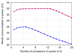
(a) $\{n_{1},n_{2},n_{3},r_{1},r_{2},r_{3}\}=\qquad$ $\{2^{12},2^{13},2^{19},2^{8},2^{13},2^{11}\}$.

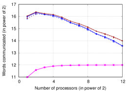
(b) $n_{1}=n_{2}=n_{3}=2^{12}$, and $r_{1}=r_{2}=r_{3}=2^{4}$.

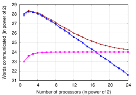
(c) $n_{1}=n_{2}=n_{3}=2^{20}$, and $r_{1}=r_{2}=r_{3}=2^{8}$.

Figure 3: Matrix and tensor communication costs in LB and Alg. 1 for different configurations. The sum of ${\sc LB(Matrix)}$ and ${\sc LB(Tensor)}$ equals to the lower bound (${\sc LB}$), and the sum of Alg. 5.1 (Matrix) and Alg. 5.1 (Tensor) equals to the upper bound (Alg. 5.1). Lower bounds are almost indistinguishable from the corresponding upper bounds.

Figure 3 shows both components, matrix and tensor communication costs, for three distinct input sizes as we vary the number of processors. In these plots, we show both algorithmic costs (upper bounds) and lower bounds, but they are indistinguishable because the largest differences in overall costs we observe are $9\%$ for Fig. 3a at $P=2^{13}$ and $13\%$ for Figures 3b and 3c at $P=2$, verifying Theorem 4.3 for these scenarios.

In Fig. 3a, the input and output tensors have varying dimensions: the input tensor is $2^{12}\times 2^{13}\times 2^{19}$ and the output is $2^{8}\times 2^{13}\times 2^{11}$. We choose these dimensions so that all five cases of the values of $A$ and $B$ are represented. For these inputs, the tensor communication cost dominates the matrix communication for all values of $P$ considered. When $P<2^{4}$, the first cases for $A$ and $B$ apply, and the algorithm selects a processor grid such that $p_{3}=P$, implying that only one tensor and two matrices are communicated. In this case, both expressions simplify to $(r+n_{1}r_{1}+n_{2}r_{2})(1-1/P)$, which is why we see initial increase as $P$ increases at the left end of the plot. For $2^{4}\leq P<2^{12}$, the second case for $A$ and the first case for $B$ apply, and the algorithm selects a processor grid with $p_{2}>1$ and $p_{3}>1$. Here, the matrix communication begins to decrease, but it is dominated by the tensor communication, which is maintained at $r(1-1/P)$. For $2^{12}\leq P$, the second case for $B$ applies, and we see that tensor communication decreases as $P$ increases (proportional to $P^{-1/2}$ as we see from the lower bound). In this regime, the algorithm is selecting grids with both $p>1$ and $q>1$ and communicating both tensors. Another transition occurs at $P=2^{16}$, switching from the second to third case of $A$, but this change in matrix cost has a negligible effect.

Figure 3b demonstrates a scenario where the matrix costs dominate the tensor costs: the input tensor is cubical with dimension $2^{12}$ and the output tensor is cubical with dimension $2^{4}$. Here we scale $P$ only up to $2^{12}$, the number of entries in the output tensor. Because the tensors are cubical, the lower bounds simplify as in Corollary 4.5, and the algorithm chooses processor grids that are as cubical as possible. For all values of $P$ in this experiment, the third case of $A$ and the first case of $B$ apply, and the algorithm selects $p_{1}\approx p_{2}\approx p_{3}$ and $q=1$. We see that the overall cost is deceasing proportional to $P^{-1/3}$ until the tensor communication cost starts to contribute more significantly.

Figure 3c considers cubical tensors with larger dimensions to show a more general pattern. For tensor dimensions $n_{i}=2^{20}$ and $r_{i}=2^{8}$, we observe a transition point where tensor communication overtakes matrix communication. Similar to the case of Figure 3b, matrix costs dominate for small $P$ and scale like $P^{-1/3}$. However, for $P\geq 2^{17}$, the tensor costs dominate the matrix costs and communication costs scale less efficiently as the first case of $B$ applies. We emphasize that for all three of these experiments, the algorithmic costs match the lower bounds nearly exactly for all values of $P$.

6.2 Comparing Algorithm 1 with TTM-in-Sequence

As mentioned previously, a Multi-TTM computation may be performed as sequence of TTM operations. In this TTM-in-Sequence approach, a single matrix is multiplied with the tensor and an intermediate tensor is computed and stored. For each remaining matrix, single-matrix TTMs are performed in sequence until the final result is computed. This approach can reduce the number of arithmetic operations compared to direct evaluation of atomic expression given in Def. 3.1. The computational cost depends (often significantly) on the order of the TTMs performed. The TTM-in-Sequence approach is parallelized in the TuckerMPI library [5]. We note that Theorem 4.3 does not apply to this parallelization, as it violates the parallel atomicity assumption.

In this section, we provide a comparison between Alg. 1 and the TTM-in-Sequence approach to show that our approach can significantly reduce communication in important scenarios without performing too much extra computation. In particular, we observe greatest benefit of Alg. 1 when $r$ is very small relative to $n$ (or vice versa) and $P$ is small relative to the ratio of $n$ and $r$. These scenarios occur in the context of computing and using Tucker decompositions for highly compressible tensors that exhibit small multilinear ranks.

The computational cost of TuckerMPI’s algorithm with cubical tensors is the same for all possible orderings of the TTMs. In our comparison, we consider that the TTMs are performed in increasing mode order. While no single communication lower bound exists for all parallel TTM-in-Sequence algorithms, we show in Subsection 6.3.2 that TuckerMPI’s algorithm attains nearly the same cost as tight matrix multiplication lower bounds [1] applied to each TTM it chooses to perform. Thus, no other parallelization of the TTM-in-Sequence approach can reduce communication without breaking the assumptions of the matrix multiplication lower bounds (e.g., using fast matrix multiplication).

The TuckerMPI parallelization uses a 3D logical processor grid with dimensions $\tilde{p_{1}}\times\tilde{p_{2}}\times\tilde{p_{3}}$. When the TTMs are performed in increasing mode order, the overall communication cost of their algorithm is

(11) $$\frac{r_{1}n_{2}n_{3}}{\tilde{p_{2}}\tilde{p_{3}}}+\frac{n_{1}r_{1}}{\tilde{p_{1}}}+\frac{r_{1}r_{2}n_{3}}{\tilde{p_{1}}\tilde{p_{3}}}+\frac{n_{2}r_{2}}{\tilde{p_{2}}}+\frac{r_{1}r_{2}r_{3}}{\tilde{p_{1}}\tilde{p_{2}}}+\frac{n_{3}r_{3}}{\tilde{p_{3}}}\phantom{\frac{r_{1}r_{2}n_{3}}{\tilde{p_{1}}\tilde{p_{3}}}}\qquad\qquad$$

$$\phantom{\frac{r_{1}r_{2}n_{3}}{\tilde{p_{1}}\tilde{p_{3}}}}\qquad\qquad-\frac{r_{1}n_{2}n_{3}+r_{1}r_{2}n_{3}+r_{1}r_{2}r_{3}+n_{1}r_{1}+n_{2}r_{2}+n_{3}r_{3}}{P},$$

as specified in [5, Section 6.3], though we include the cost of communicating the matrices (their analysis assumes the matrices are already redundantly distributed). We use exhaustive search to determine the processor grid that minimizes the cost of equation 11 in our comparisons.

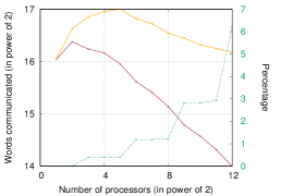
(a) $n_{i}=2^{12}$, $r_{i}=2^{4}$.

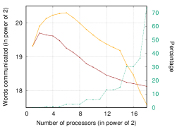
(b) $n_{i}=2^{13}$, $r_{i}=2^{6}$.

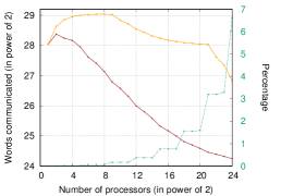
(c) $n_{i}=2^{20}$, $r_{i}=2^{8}$.

Figure 4: Communication cost comparison of Alg. 1 and TTM-in-Sequence [5]. $Comp-Overhead$ shows the percentage of computational overhead of Alg. 1 with respect to the TTM-in-Sequence approach.

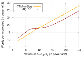
Figure 5: Comparison of Alg. 1 and the TTM-in-Sequence approach for fixed $r_{1}=r_{2}=r_{3}=2^{6}$ and $P=2^{12}$.

6.2.1 Communication Cost

To compare communications costs, we perform 4 experiments involving cubical tensors. The first three simulated evaluations consider strong scaling and are presented in Fig. 4. Two of these experiments use the same tensor dimensions as the two cubical examples in Fig. 3. The first experiment involves an input tensor of dimension $n_{i}=2^{12}$ and output dimension $r_{i}=2^{4}$ (Fig. 4a), the second has dimensions $n_{i}=2^{13}$ and $r_{i}=2^{6}$ (Fig. 4b), and the third has the largest dimensions $n_{i}=2^{20}$ and $r_{i}=2^{8}$ (Fig. 4c).

Figure 4a shows that Alg. 1 performs less communication than TTM-in-Sequence for $P\leq 2^{12}<n/r$. The largest communication reduction occurs at $P=2^{12}$ and is approximately $5\times$. In the second experiment, we see cases where TTM-in-Sequence performs less communication than Alg. 1 and in fact beats the lower bound of Theorem 4.3 (which is possible because it breaks the atomicity assumption). Algorithm 1 is more communication efficient for $P\leq 2^{16}$, achieving a speedup of up to $2\times$, but communicates more for larger $P$. In the third experiment with larger tensors, Fig. 4c demonstrates similar qualitative behavior to the first, with Alg. 1 outperforming TTM-in-Sequence and a maximum communication reduction of approximately $12\times$ at $P=2^{21}$.

In the fourth experiment, with results shown in Fig. 5, we fix the output tensor dimension $r_{i}=2^{6}$ and number of processors $P=2^{12}$ and vary the input tensor dimension $n_{i}$. We observe that for $2^{6}\leq n_{i}<2^{12}$, the TTM-in-Sequence approach communicates less data than Alg. 1. For $n_{i}\geq 2^{12}$, Alg. 1 communicates less data, and the factor of improvement is maintained at approximately $6\times$ as $n_{i}$ scales up.

6.2.2 Computation Cost

Assuming TuckerMPI uses increasing mode order, the parallel computational cost is

$$2\cdot\frac{r_{1}n_{1}n_{2}n_{3}+r_{1}r_{2}n_{2}n_{3}+r_{1}r_{2}r_{3}n_{3}}{P}=2\left(\frac{r^{1/3}n}{P}+\frac{r^{2/3}n^{2/3}}{P}+\frac{rn^{1/3}}{P}\right),$$

where the right hand side is simplified under the assumption of cubical tensors. In these experiments where $n\gg r$, Alg. 1 selects a processor grid such that $q=1$ and $p_{1}\approx p_{2}\approx p_{3}$. In this case the computation cost given in Subsection 5.1 simplifies to

$$2\left(\frac{r^{1/3}n}{P}+\frac{r^{2/3}n^{2/3}}{P^{2/3}}+\frac{rn^{1/3}}{P^{1/3}}\right).$$

Note that this cost is much smaller than $4nr/P$, the cost of evaluating equation 1 directly with computational load balance, and it is achieved by performing local computation using a TTM-in-Sequence approach.

While the first terms of the two computational cost expressions match, we observe greater computational cost from Alg. 1 in the second and third terms. These terms are lower order when $P\ll n/r$, in which case the extra computational cost of Alg. 1 is negligible. This is also validated by Fig. 4 for the first three experiments. When $P=n/r$, the extra computational cost is no more than $2\times$.

In the first three experiments, when our approach reduces communication, the extra computational costs were at most $6\%$, $30\%$, and $7\%$, respectively. The extra computation required for the greatest reductions in communication in those experiments were $6\%$, $2\%$, and $7\%$. For the fourth experiment, the extra computation is approximately $13\%$ at $n_{i}=2^{13}$, where Alg. 1 provides communication reduction, and decreases as $n_{i}$ increases.

In all these experiments, we see that when Alg. 1 provides a reduction in communication costs, the extra computational costs remain negligible.

6.3 Details for Evaluation of Our Algorithm

Here we provide more details for the simulated evaluation of our algorithm and its comparison to the TTM-in-Sequence approach. The analysis of the communication optimality of Alg. 1 did not consider integrality constraints on the processor grid dimensions. The simulated evaluation in the previous subsection considered all possible processor grid configurations using exhaustive search; we explain in Subsection 6.3.1 a more efficient process for determining an optimal grid when $P$ is a power of two. In the previous subsection, we also compare Alg. 1 against an implementation of the TTM-in-Sequence approach as implemented by TuckerMPI [5]. We argue in Subsection 6.3.2 that this implementation is nearly communication optimal given the computation that it performs, validating our comparison against it. Figure 6 presents results relevant to both Subsections 6.3.1 and 6.3.2.

6.3.1 Obtaining Integral Processor Grids for Alg. 1

In order to determine the communication cost of Alg. 1, one must determine the processor grid. Obtaining $p_{i}$ and $q_{i}$ from the procedure in Section 5 may yield non-integer values. The following procedure allows us to convert these to integers under our assumption that all parameters are powers of $2$. Recall that we consider $P=pq$ with $p=p_{1}p_{2}p_{3}$ and $q=q_{1}q_{2}q_{3}$.

If $\lfloor\log_{2}(p)+0.5\rfloor=\lfloor\log_{2}(p)\rfloor$, then we set $p=2^{\lfloor\log_{2}(p)\rfloor}$, otherwise we set $p=2^{\lceil\log_{2}(p)\rceil}$, distributing the modification evenly between $p_{1},p_{2},$ and $p_{3}$. Now, we keep $p=p_{1}p_{2}p_{3}$ constant, and convert each $p_{i}$ to an integer. We set $p_{1}=2^{\lfloor\log_{2}(p_{1})+0.5\rfloor}$ distributing the changes evenly among $p_{2}$ and $p_{3}$. To see that our new value of $p_{1}$ must still be smaller than $n_{1}$, we note that our original $p_{1}$ was less than $n_{1}$ which is a power of 2 by our assumption. If we increased $p$ in our first step, then distributing the modifications evenly between $p_{1},p_{2}$ and $p_{3}$ increased them by at most $2^{1/6}$. Thus $p_{1}\leq n_{1}$ will imply that $\lfloor\log_{2}(p_{1}\cdot 2^{1/6})+0.5\rfloor\leq\log_{2}(n_{1})$. Note that this most recent modification to $p_{1}$ changes $p_{2}$ and $p_{3}$. Then, we set $p_{2}=2^{\lfloor\log_{2}(p_{2})+0.5\rfloor}$ and adapt $p_{3}$ accordingly. A similar argument to what is used for $p_{1}$ will show that $p_{2}$ and $p_{3}$ are also not larger than their corresponding dimensions. Having completed our work on the processor dimensions associated with the first tensor, we set $q=\frac{P}{p}$ distributing the changes evenly among the $q_{i}$, then force each $q_{i}$ to be an integer following the same procedure as for the $p_{i}$.

We denote the communication cost of Alg. 1 for the grid determined using this method by Alg. 1 (fast) and the communication cost using exhaustive search by Alg. 1 (best). We note that this procedure can increase the total number of accessed elements of any variable at most $4$ times, but we see in Fig. 6 that the communication costs of both procedures are exactly the same for the examples we consider. These problems match those presented in Fig. 4.

   

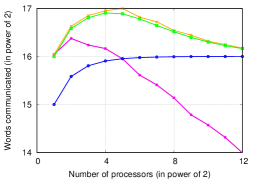
(a) $n_{i}=2^{12}$, $r_{i}=2^{4}$.

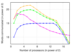
(b) $n_{i}=2^{13}$, $r_{i}=2^{6}$.

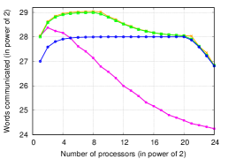
(c) $n_{i}=2^{20}$, $r_{i}=2^{8}$.

Figure 6: Communication cost comparison of Alg. 1 using best processor grid against fast method and of the TTM-in-Sequence approach implemented by TuckerMPI against the lower bounds. Alg. 1 (fast) and Alg. 1 (best) are the same for all the configurations.

6.3.2 TTM-in-Sequence Lower Bounds

Here we discuss communication lower bounds for the TTM-in-Sequence approach with cubical tensors. There has not been any proven bound for this approach other than individual bounds for each TTM (a single matrix multiply) computation, assuming the sequence of TTMs has been specified. The sum of individual bounds provides a communication lower bound for this approach. We obtain the tightest (and obtainable) lower bound for each TTM from [2], which depends on the relative matrix dimensions and number of processors, and represent the sum by $C_{LB}$(TTM-in-Seq). We also note that $C_{LB}$(TTM-in-Seq) may not be always attainable as data distributions for two successive TTMs may be non-compatible and require extra communication. When the input tensor dimensions are much larger than the output tensor dimensions, most of the computation and communication occur in the first TTM, so we also consider the communication lower bound of only that matrix multiplication, which also provides a valid lower bound for the entire TTM-in-Sequence computation. Recall that we obtain the algorithmic cost of TTM-in-Sequence by exhaustively searching for the best processor grid configuration given the communication costs specified by equation 11. Figure 6 shows a comparison of TTM-in-Seq and $C_{LB}$(TTM-in-Seq) for the tensor dimensions presented in Fig. 4. We can see that the communication costs of TTM-in-Seq are very close to $C_{LB}$(TTM-in-Seq), the largest differences are $7.9\%$ for Fig. 6a at $P=2^{5}$, $25\%$ for Fig. 6b at $P=2^{6}$, and $9.3\%$ for Fig. 6c at $P=2^{21}$. Comparing $C_{LB}$(1st TTM) and $C_{LB}$(TTM-in-Seq), we see that for these examples at least half the communication of the entire TTM-in-Sequence is required by the first TTM, and it is completely dominated by the first TTM when $P$ is large.

7 Lower Bounds of General Multi-TTM

We present our lower bound results for $d$-dimensional tensors in this section. Similar to the 3-dimensional lower bound proof, we consider a single processor that performs $1/P$th of the computation and owns at most $1/P$th of the data. We again seek to minimize the number of elements of the matrices and tensors that the processor must access or partially compute in order to execute its computation subject to the constraints of the structure of Multi-TTM by solving two independent problems, one for the matrix data and one for the tensor data.

7.1 General Constrained Optimization Problems

Here we present a generalization of Corollary 4.1 for $d$ dimensions. As before, this corollary is a direct result of Theorem 3.4. Recall the notation $N_{i}=\prod_{j=d-i+1}^{d}n_{j}$ and $R_{i}=\prod_{j=d-i+1}^{d}r_{i}$.

Corollary 7.1.

Consider the following optimization problem:

$$\min_{{\bm{\mathbf{{x}}}}}\sum_{i\in[d]}x_{i}$$

such that

$$\frac{nr}{P}\leq\prod_{i\in[d]}x_{i}\quad\text{and}\quad 0\leq x_{i}\leq n_{i}r_{i}\quad\text{for all}\quad 1\leq i\leq d,$$

where $n_{i},r_{i},P\geq 1$ and $n_{i}r_{i}\leq n_{i+1}r_{i+1}$. The optimal solution $\mathbf{x}=[{x_{1}}^{*}$ $\cdots$ ${x_{d}}^{*}]$ depends on the values of constants, yielding $d$ cases.

• If $P<\frac{N_{1}R_{1}}{n_{d-1}r_{d-1}}$, then

  $${x_{j}}^{*}=n_{j}r_{j}\quad\text{for}\quad 1\leq j\leq d-1\quad\text{and}\quad{x_{d}}^{*}=\frac{N_{1}R_{1}}{P}.$$

• If $\frac{N_{i-1}R_{i-1}}{(n_{d+1-i}r_{d+1-i})^{i-1}}\leq P<\frac{N_{i}R_{i}}{(n_{d-i}r_{d-i})^{i}}$ for some $i=2,\cdots,d-1$, then

  $${x_{j}}^{*}=n_{j}r_{j}\quad\text{for}\quad 1\leq j\leq d-i\quad\text{and}\quad{x_{d+1-i}}^{*}=\cdots={x_{d}}^{*}=\left(N_{i}R_{i}/P\right)^{1/i}.$$

• If $\frac{N_{d-1}R_{d-1}}{(n_{1}r_{1})^{d-1}}\leq P$, then

  $${x_{1}}^{*}=\cdots={x_{d}}^{*}=\left(N_{d}R_{d}/P\right)^{1/d}.$$

7.2 Communication Lower Bounds

We now present the lower bounds for the general Multi-TTM computation. We prove this by applying Corollaries 7.1 and 4.2 and extending the arguments of Theorem 4.3 in a straightforward way (though with more complicated notation).

Theorem 7.2.

Any computationally load balanced atomic Multi-TTM algorithm that starts and ends with one copy of the data distributed across processors and involves $d$-dimensional tensors with dimensions $n_{1},n_{2},\ldots,n_{d}$ and $r_{1},r_{2},\ldots,r_{d}$ performs at least $A+B-\left(\frac{n}{P}+\frac{r}{P}+\sum_{j=1}^{d}\frac{n_{j}r_{j}}{P}\right)$ sends or receives where

$$A =\begin{cases}\sum_{j=1}^{d\text{-}1}n_{j}r_{j}+\frac{N_{1}R_{1}}{P}&\text{ if }P<\frac{N_{1}R_{1}}{n_{d\text{-}1}r_{d\text{-}1}}\text{,}\\ \sum_{j=1}^{(d\text{-}i)}n_{j}r_{j}+i\left(\frac{N_{i}R_{i}}{P}\right)^{\frac{1}{i}}&\text{ if }\frac{N_{i\text{-}1}R_{i\text{-}1}}{(n_{d+1\text{-}i}r_{d+1\text{-}i})^{i\text{-}1}}\leq P<\frac{N_{i}R_{i}}{(n_{d\text{-}i}r_{d\text{-}i})^{i}}\text{,}\\ &\hfill\text{for some }2\leq i\leq d-1,\\ d\left(\frac{N_{d}R_{d}}{P}\right)^{\frac{1}{d}}&\text{ if }\frac{N_{d\text{-}1}R_{d\text{-}1}}{(n_{1}r_{1})^{d\text{-}1}}\leq P\text{.}\end{cases}$$

$$B =\begin{cases}r+\frac{n}{P}&\text{ if }P<\frac{n}{r}\text{,}\\ 2\left(\frac{nr}{P}\right)^{\frac{1}{2}}&\text{ if }\frac{n}{r}\leq P\text{.}\end{cases}$$

Proof 7.3.

Let $F$ be the set of loop indices associated with the $(d{+}1)$-ary multiplications performed by a processor. As we assumed the algorithm is computationally load balanced, $|F|=nr/P$. We define $\phi_{\bm{\mathscr{{X}}}}(F)$, $\phi_{\bm{\mathscr{{Y}}}}(F)$ and $\phi_{j}(F)$ to be the projections of $F$ onto the indices of the arrays $\bm{\mathscr{{X}}},\bm{\mathscr{{Y}}}$, and ${\bm{\mathbf{{A}}}}^{(j)}$ for $1\leq j\leq d$ which correspond to the elements of the arrays that must be accessed or partially computed by the processor.

We use Lemma 3.3 to obtain a lower bound on the number of array elements that must be accessed or partially computed by the processor. The matrix corresponding to the projections above is given by

$${\bm{\mathbf{{\Delta}}}}=\begin{bmatrix}{\bm{\mathbf{{I}}}}_{d\times d}&{\bm{\mathbf{{1}}}}_{d}&{\bm{\mathbf{{0}}}}_{d}\\ {\bm{\mathbf{{I}}}}_{d\times d}&{\bm{\mathbf{{0}}}}_{d}&{\bm{\mathbf{{1}}}}_{d}\end{bmatrix}\text{.}$$

Here ${\bm{\mathbf{{1}}}}_{d}$ and ${\bm{\mathbf{{0}}}}_{d}$ denote the $d$-dimensional vectors of all ones and zeros, respectively, and ${\bm{\mathbf{{I}}}}_{d\times d}$ denotes the $d\times d$ identity matrix. As before we define

$$\mathcal{C}=\big{\{}{\bm{\mathbf{{s}}}}={[s_{1}\ \cdots\ s_{d+2}]^{\sf T}:0\leq s_{i}\leq 1\text{ for }i=1,2,\cdots,d+2\text{ and }}{\bm{\mathbf{{\Delta}}}}\cdot{\bm{\mathbf{{s}}}}\geq{\bm{\mathbf{{1}}}}\big{\}}\text{.}$$

We recall that ${\bm{\mathbf{{1}}}}$ represents a vector of all ones. As in the proof of Theorem 4.3, ${\bm{\mathbf{{\Delta}}}}$ is not full rank, so we again consider each vector ${\bm{\mathbf{{v}}}}\in\mathcal{C}$ such that ${\bm{\mathbf{{\Delta}}}}\cdot{\bm{\mathbf{{v}}}}={\bm{\mathbf{{1}}}}$. Such a vector ${\bm{\mathbf{{v}}}}$ is of the form $\begin{bmatrix}a&\cdots&a&1-a&1-a\end{bmatrix}$ where $0\leq a\leq 1$. Thus, we obtain

$$\frac{nr}{P}\leq\Big{(}\prod_{j\in[d]}|\phi_{j}(F)|\Big{)}^{a}\big{(}|\phi_{\bm{\mathscr{{X}}}}(F)||\phi_{\bm{\mathscr{{Y}}}}(F)|\big{)}^{1\text{-}a}\text{.}$$

Similar to the 3D case, the above constraint is equivalent to $\frac{nr}{P}\leq\prod_{j\in[d]}|\phi_{j}(F)|$ and $\frac{nr}{P}\leq|\phi_{\bm{\mathscr{{X}}}}(F)||\phi_{\bm{\mathscr{{Y}}}}(F)|$.

Clearly a projection onto an array can not be larger than the array itself, thus $|\phi_{\bm{\mathscr{{X}}}}(F)|\leq n$, $|\phi_{\bm{\mathscr{{Y}}}}(F)|\leq r$, and $|\phi_{j}(F)|\leq n_{j}r_{j}$ for $1\leq j\leq d$.

As the constraints related to the projections of matrices and tensors are disjoint, we solve them separately and then sum the results to get a lower bound on the number of elements that must be accessed or partially computed by the processor. We obtain a lower bound on $A$, the number of relevant elements of the matrices by using Corollary 7.1, and a lower bound on $B$, the number of relevant elements of the tensors by using Corollary 4.2. By summing both, we get the positive terms of the lower bound.

To bound the sends or receives, we consider how much data the processor could have had at the beginning or at the end of the computation. Assuming there is exactly one copy of the data at the beginning and at the end of the computation, there must exist a processor which owns at most $1/P$ of the elements of the arrays at the beginning or at the end of the computation. By employing the previous analysis, this processor must access or partially compute $A+B$ elements of the arrays, but can only own $\frac{n}{P}+\frac{r}{P}+\sum_{j\in[d]}\frac{n_{j}r_{j}}{P}$ elements of the arrays. Thus it must perform the specified amount of sends or receives.

8 Parallel Algorithm for General Multi-TTM

We present a parallel algorithm to compute $d$-dimensional Multi-TTM in Alg. 2, which is analogous to Alg. 1. We organize $P$ processors into a $2d$-dimensional logical processor grid with dimensions $p_{1}\times\cdots\times p_{d}\times q_{1}\times\cdots\times q_{d}$. As before, we consider that $\forall i\in[d]$, $p_{i}$ and $q_{i}$ evenly divide $n_{i}$ and $r_{i}$, respectively. A processor coordinate is represented as $(p_{1}^{\prime},\cdots,p_{d}^{\prime},q_{1}^{\prime},\cdots,q_{d}^{\prime})$, where $\forall i\in[d]$, $1\leq p_{i}^{\prime}\leq p_{i}$ and $1\leq q_{i}^{\prime}\leq q_{i}$.

Algorithm 2 Parallel Atomic d-dimensional Multi-TTM

0:  $\bm{\mathscr{{X}}}$, ${\bm{\mathbf{{A}}}}^{(1)}$, $\cdots$, ${\bm{\mathbf{{A}}}}^{(d)}$, $p_{1}\times\cdots\times p_{d}\times q_{1}\times\cdots\times q_{d}$ logical processor grid

0:  $\bm{\mathscr{{Y}}}$ such that $\bm{\mathscr{{Y}}}=\bm{\mathscr{{X}}}\times_{1}{{\bm{\mathbf{{A}}}}^{(1)}}^{\sf T}\cdots\times_{d}{{\bm{\mathbf{{A}}}}^{(d)}}^{\sf T}$

1:  $(p_{1}^{\prime},\cdots,p_{d}^{\prime},q_{1}^{\prime},\cdots,q_{d}^{\prime})$ is my processor id

2:  //All-gather input tensor $\bm{\mathscr{{X}}}$

3:  $\bm{\mathscr{{X}}}_{p_{1}^{\prime}\cdots p_{d}^{\prime}}$ = All-Gather($\bm{\mathscr{{X}}}$, $(p_{1}^{\prime},\cdots,p_{d}^{\prime},*,\cdots,*)$)

4:  //All-gather all input matrices

5:  for $i=1,\cdots,d$ do

6:     ${\bm{\mathbf{{A}}}}^{(i)}_{p_{i}^{\prime}q_{i}^{\prime}}$ = All-Gather(${\bm{\mathbf{{A}}}}^{(i)}$, $(*,\cdots,*,p_{i}^{\prime},*\cdots,*,q_{i}^{\prime},*)$)

7:  end for

8:  //Perform local computations in a temporary tensor $\bm{\mathscr{{T}}}$

9:  $\bm{\mathscr{{T}}}$ = Local-Multi-TTM($\bm{\mathscr{{X}}}_{p_{1}^{\prime}\cdots p_{d}^{\prime}}$, ${\bm{\mathbf{{A}}}}^{(1)}_{p_{1}^{\prime}q_{1}^{\prime}}$,$\cdots$, ${\bm{\mathbf{{A}}}}^{(d)}_{p_{d}^{\prime}q_{d}^{\prime}}$)

10:  //Reduce-scatter the output tensor in $\bm{\mathscr{{Y}}}_{q_{1}^{\prime}\cdots q_{d}^{\prime}}$

11:  Reduce-Scatter($\bm{\mathscr{{Y}}}_{q_{1}^{\prime}\cdots q_{d}^{\prime}}$, $\bm{\mathscr{{T}}}$, $(*,\cdots,*,q_{1}^{\prime},\cdots,q_{d}^{\prime})$)

Here we discuss our data distribution model for Alg. 2, which is similar to that of Alg. 1. $\bm{\mathscr{{X}}}_{p_{1}^{\prime}\cdots p_{d}^{\prime}}$ and $\bm{\mathscr{{Y}}}_{q_{1}^{\prime}\cdots q_{d}^{\prime}}$ denote the subtensors of $\bm{\mathscr{{X}}}$ and $\bm{\mathscr{{Y}}}$ owned by processors $(p_{1}^{\prime},\cdots,p_{d}^{\prime},*,\cdots,*)$ and $(*,\cdots,*,q_{1}^{\prime},\cdots,q_{d}^{\prime})$, respectively. ${\bm{\mathbf{{A}}}}^{(i)}_{p_{i}^{\prime}q_{i}^{\prime}}$ denotes the submatrix of ${\bm{\mathbf{{A}}}}^{(i)}$ owned by processors $(*,\cdots,*,p_{i}^{\prime},*,\cdots,*,q_{i}^{\prime},*,\cdots,*)$. We impose that there is one copy of data in the system at the beginning and the end of the computation, and each subarray is distributed evenly among the set of processors which own the data.

When Alg. 2 completes, $\bm{\mathscr{{Y}}}_{q_{1}^{\prime}\cdots q_{d}^{\prime}}$ is distributed evenly among processors $(*,\cdots,*,\linebreak q_{1}^{\prime},\cdots,q_{d}^{\prime})$. We recall that $\prod_{i=1}^{d}p_{i}$ and $\prod_{i=1}^{d}q_{i}$ are denoted by $p$ and $q$, respectively.

8.1 Cost Analysis

Now we analyze computation and communication costs of the algorithm. As before, the local Multi-TTM computation in Line 9 can be performed as a sequence of TTM operations to mininimize the number of arithmetic operations. Assuming the TTM operations are performed in their order, first with ${\bm{\mathbf{{A}}}}^{(1)}$, then with ${\bm{\mathbf{{A}}}}^{(2)}$, and so on until the last is performed with ${\bm{\mathbf{{A}}}}^{(d)}$, then each processor performs $\sum_{k=1}^{d}\left(2\prod_{i=1}^{k}\frac{r_{i}}{q_{i}}\prod_{j=k}^{d}\frac{n_{j}}{p_{j}}\right)$ operations. In Line 11, each processor also performs $(1-\frac{q}{P})\frac{r}{q}$ computations due to the Reduce-Scatter operation.

Communication occurs only in All-Gather and Reduce-Scatter collectives in Lines 3, 6, and 11. Line 3 specifies $p$ All-Gathers over disjoint sets of $\frac{P}{p}$ processors, Line 6 specifies ${p_{i}q_{i}}$ All-Gathers over disjoint sets of $\frac{P}{p_{i}q_{i}}$ processors in the $i$th loop iteration, and Line 11 specifies $q$ Reduce-Scatters over disjoint sets of $\frac{P}{q}$ processors. Each processor is involved in one All-Gather involving the input tensor, $d$ All-Gathers involving input matrices and one Reduce-Scatter involving the output tensor.

As before, we assume bandwidth and latency optimal algorithms are used for the All-Gather and Reduce-Scatter collectives. Hence the bandwidth costs of the All-Gather operations are $(1-\frac{p}{P})\frac{n}{p}$ for Line 3, and $\sum_{i=1}^{d}(1-\frac{p_{i}q_{i}}{P})\frac{n_{i}r_{i}}{p_{i}q_{i}}$ for the $d$ iterations of Line 6. The bandwidth cost of the Reduce-Scatter operation in Line 11 is $(1-\frac{q}{P})\frac{r}{q}$. Hence the overall bandwidth cost of Alg. 2 along the critical path is $\frac{n}{p}+\frac{r}{q}+\sum_{i=1}^{d}\frac{n_{i}r_{i}}{p_{i}q_{i}}-\left(\frac{n+r+\sum_{i=1}^{d}n_{i}r_{i}}{P}\right)$. The latency costs are $\log_{2}\left(\frac{P}{p}\right)$ and $\log_{2}\left(\frac{P}{q}\right)$ for Lines 3 and 11 respectively, and $\sum_{i=1}^{d}\log_{2}\left(\frac{P}{p_{i}q_{i}}\right)$ for the $d$ iterations of Line 6. Thus the overall latency cost of Alg. 2 along the critical path is $\log_{2}\left(\frac{P}{p}\right)+\sum_{i=1}^{d}\log_{2}\left(\frac{P}{p_{i}q_{i}}\right)+\log_{2}\left(\frac{P}{q}\right)=d\log_{2}(P).$

We can prove the following theorem by extending the arguments of Theorem 5.1.

Theorem 8.1.

There exist $p_{i},q_{i}$ with $1\leq p_{i}\leq n_{i},1\leq q_{i}\leq r_{i}$ for $i=1,\cdots,d$ such that Alg. 2 is communication optimal to within a constant factor.

Proof 8.2.

As we did previously, we break our analysis into 2 scenarios which are further broken down into all possible cases.

In each case, we obtain $\hat{p_{j}}$ and $\hat{q_{j}}$ such that the terms in the communication cost match the corresponding lower bound terms and satisfy at least one of the two sets of constraints, $1\leq\hat{p_{j}}\leq n_{j}$, $1\leq\hat{q_{j}}$ or $1\leq\hat{q_{j}}\leq r_{j}$, $1\leq\hat{p_{j}}$ for $1\leq j\leq d$. We handle all cases of both scenarios together in the end, and adapt these values to get $p_{j}$ and $q_{j}$ which respect both lower and upper bounds for all values of $j$. Then we determine how much additional communication may be required. We denote $\prod_{i=1}^{d}\hat{p_{i}}$ and $\prod_{i=1}^{d}\hat{q_{i}}$ by $\hat{p}$ and $\hat{q}$.

$\bullet$ Scenario I $\left(P<\frac{n}{r}\right)$: This scenario corresponds to the first case of the tensor term in ${\sc LB}$. Thus, we set $\hat{p_{j}},\hat{q_{j}}$ in such a way that the tensor terms in the communication cost match the tensor terms of ${\sc LB}$:

(12) $$\hat{p}=P,\hat{q}=1.$$

This implies $\hat{q_{j}}=1$ for $1\leq j\leq d$. We break this scenario into $d$ cases parameterized by $I$: $\frac{N_{I-1}R_{I-1}}{(n_{d-I+1}r_{d-I+1})^{I-1}}\leq P<\min\big{\{}\frac{N_{I}R_{I}}{(n_{d-I}r_{d-I})^{I}},\frac{n}{r}\big{\}}$. The cases degenerate to $P<\min\big{\{}\frac{N_{1}R_{1}}{n_{d-1}r_{d-1}},\frac{n}{r}\big{\}}$, when $I=1$, and $\frac{N_{d-1}R_{d-1}}{(n_{1}r_{1})^{d-1}}\leq P<\frac{n}{r}$ when $I=d$.

Setting the matrix communication costs to the matrix terms of the lower bound in the corresponding cases yields

(13) $$\frac{n_{j}r_{j}}{\hat{p_{j}}\hat{q_{j}}}=n_{j}r_{j}\text{ if }1\leq j\leq d-I,\qquad\frac{n_{j}r_{j}}{\hat{p_{j}}\hat{q_{j}}}=\left(\frac{N_{I}R_{I}}{P}\right)^{\frac{1}{I}}\text{ if }d-I<j\leq d.$$

Thus, $\hat{q_{j}}=1$ for all $1\leq j\leq d$, $\hat{p_{j}}=1$ if $1\leq j\leq d-I$ and $\hat{p_{j}}=n_{j}r_{j}\big{(}\frac{P}{N_{I}R_{I}}\big{)}^{\frac{1}{I}}$ if $d-I<j\leq d$ to satisfy equations 12 and 13. Note that when $I=1$, $p_{d}=P\geq 1$, and for the other values of $I$, $p_{j}\geq 1$ because $n_{1}r_{1}\leq\cdots\leq n_{d}r_{d}$ and $\frac{N_{I-1}R_{I-1}}{(n_{d-I+1}r_{d-I+1})^{I-1}}\leq P$. Additionally we have that $1=\hat{q_{j}}<r_{j}$ for $1\leq j\leq d$. However, we are not able to ensure $\hat{p_{j}}\leq n_{j}$ when $d-I<j\leq d$. We will handle all cases of both scenarios together as they require the same analysis.

$\bullet$ Scenario II $\left(\frac{n}{r}\leq P\right)$: This scenario corresponds to the second case of the tensor term in ${\sc LB}$. Thus, we set $\hat{p_{i}},\hat{q_{i}}$ in such a way that

(14) $$\frac{n}{\hat{p}}=\frac{r}{\hat{q}}=\left(\frac{nr}{P}\right)^{1/2}.$$

Again, we break this scenario into $d$ cases parameterized by $I$:

$$\max\left\{\frac{N_{I-1}R_{I-1}}{(n_{d-I+1}r_{d-I+1})^{I-1}},\frac{n}{r}\right\}\leq P<\frac{N_{I}R_{I}}{(n_{d-I}r_{d-I})^{I}}\;\cdot$$

The cases degenerate to $P<\frac{N_{1}R_{1}}{n_{d-1}r_{d-1}}$, when $I=1$, and $\max\left\{\frac{N_{d-1}R_{d-1}}{(n_{1}r_{1})^{d-1}},\frac{n}{r}\right\}\leq P$ when $I=d$.

Setting the matrix communication costs to match the corresponding matrix terms in the lower bound yields

(15) $$\frac{n_{j}r_{j}}{\hat{p_{j}}\hat{q_{j}}}=n_{j}r_{j}\text{ if }1\leq j\leq d-I,\qquad\frac{n_{j}r_{j}}{\hat{p_{j}}\hat{q_{j}}}=\left(\frac{N_{I}R_{I}}{P}\right)^{\frac{1}{I}}\text{ if }d-I<j\leq d.$$

Thus we set $\hat{q_{j}}=\hat{p_{j}}=1$ for all $1\leq j\leq d-I$. When $2\leq I\leq d$, the equations above do not uniquely determine $\hat{p_{j}},\hat{q_{j}}$ for $d-I<j\leq d$. However, setting $\hat{p_{j}}=n_{j}\left(\frac{nP}{rN_{I}^{2}}\right)^{1/2I}$ and $\hat{q_{j}}=r_{j}\left(\frac{rP}{nR_{I}^{2}}\right)^{1/2I}$ for $d-I<j\leq d$ satisfies equations 14, 15 in all cases. Note that we cannot ensure lower and upper bounds on $\hat{p_{j}}$ and $\hat{q_{j}}$. We now look for new solutions to the equations twice. First, we ensure that all lower bounds are respected, i.e., $1\leq\hat{p_{j}}$ and $1\leq\hat{q_{j}}$, and then we guarantee that all upper bounds of $\hat{p_{j}}$ or $\hat{q_{j}}$ are satisfied, i.e., $\hat{p_{j}}\leq n_{j}$ or $\hat{q_{j}}\leq r_{j}$.

As we compared communication cost of each term with its corresponding lower bound to obtain $\hat{p_{j}}$ and $\hat{q_{j}}$, we have $1\leq\hat{p_{j}}\hat{q_{j}}\leq n_{j}r_{j}$ for $1\leq j\leq d$, $1\leq\hat{p}\leq n$ and $1\leq\hat{q}\leq r$ in all $d$ cases. However, we may not have $1\leq\hat{p_{j}}$ or $1\leq\hat{q_{j}}$ for some $j$. We now seek new solutions that are all greater than $1$. First we will increase all $\hat{q_{j}},\hat{p_{j}}$ that are less than $1$ in a way that preserves products $\hat{p_{j}}\hat{q_{j}}$ but does not preserve $\hat{p}$ and $\hat{q}$. Then we will adjust $\hat{p_{j}}$ and $\hat{q_{j}}$ to force the products $\hat{p}$ and $\hat{q}$ back to their initial values.

Let $q^{b}$ denote the product of all $\hat{q_{j}}$ such that $\hat{q_{j}}<1$, and $p^{b}$ denote the product of all $\hat{p_{j}}$ such that $\hat{p_{j}}<1$. Without loss of generality, if $q^{b}\leq p^{b}$, set $a=1$ $\hat{p}^{orig}=\hat{p}$, and $\hat{q}^{orig}=\hat{q}$. We perform the following updates:
Looping over the index $j$ from 1 to $d$, if $\hat{q_{j}}<1$ then set $a=a\cdot\hat{q_{j}},\hat{p_{j}}=\hat{p_{j}}\hat{q_{j}},\hat{q_{j}}=1$; else if $\hat{p_{j}}<1$ then set $a=a/\hat{p_{j}},\hat{q_{j}}=\hat{p_{j}}\hat{q_{j}},\hat{p_{j}}=1.$ This step preserves all products $\hat{p_{j}}\hat{q_{j}}$ and enforces $1\leq\hat{p_{j}},1\leq\hat{q_{j}}$ for $1\leq j\leq d$, but it does not preserve $\hat{p},\hat{q}$. At the end of this step, we have $a=q^{b}/p^{b}<1$, $\hat{p}=a\cdot\hat{p}^{orig}$, and $\hat{q}=\hat{q}^{orig}/a$. In order to force $\hat{p}$ and $\hat{q}$ to match their initial values, we decrease some $\hat{q_{j}}$ in such a way that $\hat{q}$ is decreased by a factor of $a$. This is possible because $1\leq\hat{q}^{orig}=a\cdot\hat{q}$. Looping over the index $j$ from 1 to $d$, if $\hat{q_{j}}>1$ then set $\hat{q_{j}}^{prev}=\hat{q_{j}},\hat{q_{j}}=\max(1,a\cdot\hat{q_{j}}),a=a\left(\frac{\hat{q_{j}}^{prev}}{\hat{q_{j}}}\right),\hat{p_{j}}=\hat{p_{j}}\left(\frac{\hat{q_{j}}^{prev}}{\hat{q_{j}}}\right)$. At the end of this step, $\hat{q}$ has been decreased by a factor of $q^{b}/p^{b}$, $\hat{p_{j}}\hat{q_{j}}$ were all preserved, and thus, $\hat{p}$ has been increased by a factor of $p^{b}/q^{b}$, hence $\hat{q}=\hat{q}^{orig}$ and $\hat{p}=\hat{p}^{orig}$. After the above updates, we have $1\leq\hat{p_{j}},1\leq\hat{q_{j}}$ for $1\leq j\leq d$, and the products match the initial products thus are valid solutions to the original equations. If $p_{b}<q_{b}$ we would perform the same process, but changing the actions on the $\hat{q_{j}}$ to be performed on the $\hat{p_{j}}$ and vice versa.

We now handle upper bounds of $\hat{p_{j}}$ and $\hat{q_{j}}$. If $\exists j,k$ such that $\hat{p_{j}}>n_{j}$ and $\hat{q_{k}}>r_{k}$, we again seek new solutions such that all $\hat{p_{j}}$ or all $\hat{q_{j}}$ satisfy upper bounds while respecting lower bounds of all variables. Let $p^{t}$ and $q^{t}$ denote the products of all $\hat{p_{j}}$ and $\hat{q_{j}}$, respectively, such that $\hat{p_{j}}\hat{q_{j}}\neq 1$. As $\forall j,1\leq\hat{p_{j}}\hat{q_{j}}\leq n_{j}r_{j}$, therefore $p^{t}$ is not more than the product of the corresponding $n_{j}$ and/or $q^{t}$ is not more than the product of the corresponding $r_{j}$. If the first constraint is satisfied, then we perform the following updates:
Looping over the index $j$ from 1 to $d$, if $p^{t}>1$ and $\hat{p_{j}}\hat{q_{j}}\neq 1$ then set $a=\hat{p_{j}}\hat{q_{j}},\hat{p_{j}}=\min(p^{t},n_{j}),\hat{q_{j}}=\frac{a}{\hat{p_{j}}},p^{t}=\frac{p^{t}}{\hat{p_{j}}}$. After the above updates, we have $1\leq\hat{p_{j}}\leq n_{j},1\leq\hat{q_{j}}$ for $1\leq j\leq d$, and $\hat{p_{j}}\hat{q_{j}}$, $\hat{p}$ and $\hat{q}$ are back to their original values. If the first constraint is not satisfied, we would perform the same process on $\hat{q_{j}}$ instead of $\hat{p_{j}}$.

Now for all cases of both scenarios, we know that $1\leq\hat{p}_{j}$ and $1\leq\hat{q_{j}}$ for $1\leq j\leq d$, and either $\hat{p}_{j}\leq n_{j}$ for $1\leq j\leq d$ or $\hat{q_{j}}\leq r_{j}$ for $1\leq j\leq d$. It remains to adapt $\hat{p}_{j}$ and $\hat{q}_{j}$ such that both $\hat{p}_{j}\leq n_{j}$ and $\hat{q}_{j}\leq r_{j}$ for $1\leq j\leq d$. We obtain $p_{1},\ldots,p_{d},q_{1},\ldots,q_{d}$ from $\hat{p_{j}}$ and $\hat{q_{j}}$ such that $p_{1}\cdots p_{d}=\hat{p}$ and $q_{1}\cdots q_{d}=\hat{q}$. The intuition is to maintain the tensor communication terms in the lower bound.

Initially, we set $p_{j}=\hat{p}_{j}$ and $q_{j}=\hat{q}_{j}$ for $1\leq j\leq d$. If $1\leq p_{j}\leq n_{j}$ and $1\leq q_{j}\leq r_{j}$ for $1\leq j\leq d$, then $\sum_{j\in[d]}\frac{n_{j}r_{j}}{p_{j}q_{j}}=\sum_{j\in[d]}\frac{n_{j}r_{j}}{\hat{p_{j}}\hat{q_{j}}}$ and the communication cost exactly matches the lower bound. Otherwise, we adapt the values and determine the effects on the matrix communication costs. We recall that due of our particular selections of $\hat{p_{j}}$ and $\hat{q_{j}}$, $\nexists j,\ell\in[d]$ such that $\hat{p_{j}}>n_{j}$ and $\hat{q_{\ell}}>r_{\ell}$. If $\hat{p}_{j}>n_{j}$ for some $j\in[d]$, then we iterate over the index $j$ from $d$ to 1 setting $p_{j}=\min\left\{n_{j},\frac{\hat{p}}{\prod_{\ell\in[d]-\{j\}}p_{\ell}}\right\}$. We iterate again from $d$ to 1 with the same expression. Iterating twice ensures that all updates are visible to all $p_{j}$.

Now we assess how much additional communication is required for the matrices. As $\hat{p_{j}}>n_{j}$ for some $j$, it must be the case that $\hat{p}\geq 2$. Thus

$$\sum_{j\in[d]}\frac{n_{j}r_{j}}{p_{j}q_{j}} \leq\sum_{j\in[d]}\max\left\{\frac{n_{j}r_{j}}{\hat{p_{j}}\hat{q_{j}}},\frac{r_{j}}{\hat{q_{j}}}\right\}$$

$$=\sum_{j\in[d]}\Big{(}\frac{n_{j}r_{j}}{\hat{p_{j}}\hat{q_{j}}}+\frac{r_{j}}{\hat{q_{j}}}-\min\big{\{}\frac{n_{j}r_{j}}{\hat{p_{j}}\hat{q_{j}}},\frac{r_{j}}{\hat{q_{j}}}\big{\}}\Big{)}$$

$$<\sum_{j\in[d]}\left(\frac{n_{j}r_{j}}{\hat{p_{j}}\hat{q_{j}}}+\frac{r_{j}}{\hat{q_{j}}}\right)-(d-1)$$

$$\leq\sum_{j\in[d]}\frac{n_{j}r_{j}}{\hat{p_{j}}\hat{q_{j}}}+\frac{r}{\hat{q}}$$

$$<\sum_{j\in[d]}\frac{n_{j}r_{j}}{\hat{p_{j}}\hat{q_{j}}}+2\left(\frac{r}{\hat{q}}-\frac{r}{\hat{p}\hat{q}}\right)$$

$$=\sum_{j\in[d]}\frac{n_{j}r_{j}}{\hat{p_{j}}\hat{q_{j}}}+2\left(\frac{r}{\hat{q}}-\frac{r}{P}\right)\text{.}$$

Similarly, if $\exists j\in[d]$ such that $\hat{q_{j}}>r_{j}$, the same update can be performed to the $q_{j}$, and we obtain $\sum_{j\in[d]}\frac{n_{j}r_{j}}{p_{j}q_{j}}<\sum_{j\in[d]}\frac{n_{j}r_{j}}{\hat{p_{j}}\hat{q_{j}}}+2\left(\frac{n}{\hat{p}}-\frac{n}{P}\right)$.

Therefore, $\sum_{j\in[d]}\frac{n_{j}r_{j}}{p_{j}q_{j}}+\frac{r}{q}+\frac{n}{p}-{\sc O}\leq 3\left(\sum_{j\in[d]}\frac{n_{j}r_{j}}{\hat{p_{j}}\hat{q_{j}}}+\frac{r}{\hat{q}}+\frac{n}{\hat{p}}-{\sc O}\right)=3{\sc LB}$.

8.2 Simulated Evaluation

Similar to Section 6, we compare communication costs of our algorithm and a TTM-in-Sequence approach implemented in the TuckerMPI library. We again restrict to cases where all dimensions are powers of $2$, and vary the number of processors $P$ from $2$ to ${\sc P_{\max}}$ in multiples of $2$, where ${\sc P_{\max}}=\min\{n_{1}r_{1},\cdots,n_{d}r_{d},n,r\}$.

Like Section 6, we look at all possible processor grid dimensions and represent the minimum communication costs of our algorithm and TuckerMPI algorithm by Alg. 2 (best) and TTM-in-Seq, respectively. The TTM-in-Sequence approach described in [5] organizes $P$ in a $d$-dimensional $\tilde{p_{1}}\times\cdots\times\tilde{p_{d}}$ logical processor grid. Assuming TTMs are performed in increasing mode order, the overall communication cost of this algorithm is

$$\frac{r_{1}n_{2}\cdots n_{d}}{\frac{P}{\tilde{p_{1}}}}+\frac{r_{1}r_{2}n_{3}\cdots n_{d}}{\frac{P}{\tilde{p_{2}}}}+\cdots+\frac{r_{1}r_{2}\cdots r_{d}}{\frac{P}{\tilde{p_{d}}}}-\frac{r_{1}n_{2}\cdots n_{d}+r_{1}r_{2}n_{3}\cdots n_{d}+\cdots+r_{1}r_{2}\cdots r_{d}}{P}$$

$$\qquad\qquad+\frac{n_{1}r_{1}}{\tilde{p_{1}}}+\cdots+\frac{n_{d}r_{d}}{\tilde{p_{d}}}-\frac{n_{1}r_{1}+\cdots+n_{d}r_{d}}{P}.$$

The first line corresponds to tensor communication and the second line corresponds to matrix communication. As mentioned earlier, the TTM-in-Sequence approach forms a tensor after each TTM computation. Each positive term of the first line corresponds to the number of entries of such a tensor partially computed by a processor in TuckerMPI.

   

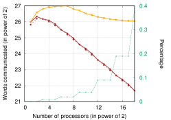
(a) $n_{1}=n_{2}=n_{3}=2^{20},r_{1}=r_{2}=r_{3}=2^{6}$

(b) $n_{1}=n_{2}=n_{3}=n_{4}=2^{20},r_{1}=r_{2}=r_{3}=r_{4}=2^{6}$

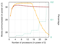
(c) $n_{1}=\cdots=n_{5}=2^{20},r_{1}=\cdots=r_{5}=2^{6}$

       

Figure 7: Communication cost comparison of Alg. 2 and the TTM-in-Sequence approach implemented by the TuckerMPI library. Note that ${\sc LB}$ is a communication lower bound for atomic Multi-TTM algorithms, not for the TTM-in-Sequence approach. Communication cost of our approach (Alg. 2 (best)) is very close to the lower bound (${\sc LB}$).

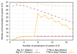
(a) $n_{1}=n_{2}=n_{3}=2^{20},r_{1}=r_{2}=r_{3}=2^{6}$

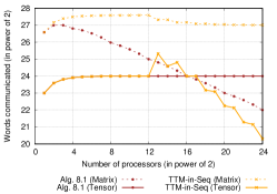
(b) $n_{1}=n_{2}=n_{3}=n_{4}=2^{20},r_{1}=r_{2}=r_{3}=r_{4}=2^{6}$

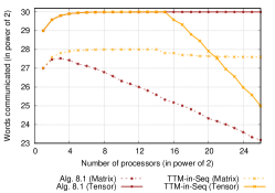
(c) $n_{1}=\cdots=n_{5}=2^{20},r_{1}=\cdots=r_{5}=2^{6}$

       

Figure 8: Matrix and Tensor communication costs in Alg. 2 and the TTM-in-Sequence approach.

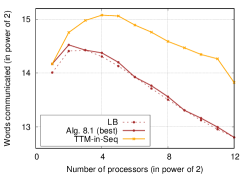
(a) $n_{1}=n_{2}=n_{3}=2^{10},r_{1}=r_{2}=r_{3}=2^{4}$

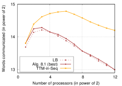
(b) $n_{1}=n_{2}=n_{3}=n_{4}=2^{10},r_{1}=r_{2}=r_{3}=r_{4}=2^{3}$

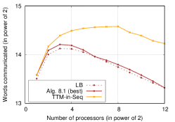
(c) $n_{1}=\cdots=n_{6}=2^{10},r_{1}=\cdots=r_{6}=2^{2}$

       

Figure 9: Communication cost comparison of Alg. 2 and the TTM-in-Sequence approach for 3/4/6-dimensional Multi-TTM computations.

We again look at cases where the input tensors are large and the output tensors are small. Figure 7 shows comparison of Alg. 2 (best) and TTM-in-Seq with our communication lower bounds (${\sc LB}$) for 3/4/5-dimensional Multi-TTM computations. For $P=2$, both approaches perform the same amount of communication. After that, the total number of accessed elements in both approaches decreases, however the rate of owned elements decreases at the faster rate. Hence we see slight increase in both curves. This behavior continues roughly till $2^{n_{i}-r_{i}}$ processors for TTM-in-Seq curve. In this region, the TTM-in-Sequence approach selects $\tilde{p_{1}}=\cdots=\tilde{p_{d-1}}=1$ and $\tilde{p_{d}}=P$, and our algorithm selects $p_{1}\approx\cdots\approx p_{d}$ and $q_{1}=\cdots=q_{d}=1$. These processor grid dimensions result in the same tensor communication cost for both approaches. However our approach reduces matrix communication cost roughly $(1-\frac{1}{d})P^{\frac{1}{d}}$ times, hence it is better than the TTM-in-Sequence approach. Fig. 8 shows the distribution of matrix and tensor communication costs in both approaches. In general, our approach significantly minimizes the matrix communication costs in all the plots and is better when the number of the entries in the output tensor is less than that of the matrices. When the communication cost is dominated by the output tensor, our approach is outperformed by the TTM-in-Sequence approach, which is the case in Fig. 7c.

The parallel computational cost of TuckerMPI with cubical tensors is

$$2\left(\frac{r^{\frac{1}{d}}n}{P}+\frac{r^{\frac{2}{d}}n^{\frac{d-1}{d}}}{P}+\cdots+\frac{rn^{\frac{1}{d}}}{P}\right).$$

When $n\gg r$, Alg. 2 selects a processor grid such that $q=1$ and $p_{1}\approx p_{2}\approx\cdots\approx p_{d}$. In this case the computation cost given in Subsection 8.1 simplifies to

$$2\left(\frac{r^{\frac{1}{d}}n}{P}+\frac{r^{\frac{2}{d}}n^{\frac{d-1}{d}}}{P^{\frac{d-1}{d}}}+\cdots+\frac{rn^{\frac{1}{d}}}{P^{\frac{1}{d}}}\right).$$

While the first terms of the two computational cost expressions match, we observe greater computational cost from Alg. 2 in the remaining terms. These terms are lower order when $P\ll n/r$, in which case the extra computational cost of Alg. 2 is negligible. We plot computational overheads of our algorithm, with $Comp-Overhead$ label, in Fig. 7. We can note that the overheads are negligible (less than 0.5%) for the considered experiments.

Now we consider a different set of experiments. Here the number of entries in the input tensor is $(2^{10})^{d}$ for $d$-dimensional computations. We fix the number of entries in the output tensor to $2^{12}$ and present comparisons of the considered approaches in Figure 9 for 3/4/6-dimensional Multi-TTM computations. These dimensions allow both tensors to be cubical. As the number of entries in the matrices are greater than the number of entries in the output tensor, our approach is always superior to the TTM-in-Sequence approach.

Our results are consistent with what we observe for $3$-dimensional Multi-TTM computations in Section 6. When the input tensor is much larger than the output tensor and the number of entries in the output tensor is less than that of the matrices, our algorithm significantly reduces communication compared to the TTM-in-Sequence approach. As in the 3D case, when $P\ll n/r$, the extra computation is negligible when the TTM-in-Sequence approach is used locally to reduce computation.

9 Conclusions

In this work, we establish communication lower bounds for the parallel Multi-TTM computation and present an optimal parallel algorithm that organizes the processors in a $2d$-dimensional grid for $d$-dimensional tensors. By judiciously selecting the processor grid dimensions, we prove that our algorithm attains the lower bounds to within a constant factor. To verify the theoretical analysis, we simulate Multi-TTM computations using a variety of values for the number of processors, $P$, the dimension, $d$, and sizes, $n_{i}$ and $r_{i}$; compute the communication costs of our algorithm corresponding to each simulation; and compute the optimal communication cost provided by the theoretical lower bound. These simulations show that the communication costs of the proposed algorithm are close to optimal. When one of the tensors is much larger than the other tensor, which is typical in compression algorithms based on the Tucker decomposition, our algorithm significantly reduces communication costs over the conventional approach of performing the computation as a sequence of tensor-times-matrix operations.

Motivated by the simulated communication cost comparisons, our next goal is to implement the parallel atomic algorithm and verify the performance improvement in practice. Further, because neither the atomic or TTM-in-sequence approach is always superior in terms of communication, we wish to explore hybrid algorithms to account for significant dimension reduction in some modes but modest reduction in others. Given the computation and communication capabilities of a parallel platform, it would also be interesting to study the computation-communication tradeoff for these two approaches and how to minimize the overall execution time in practice. Finally, this work considers that each processor has enough memory. A natural extension is to study communication lower bounds for Multi-TTM computations with limited memory sizes.

Appendix A Proof of Theorem 3.4

In this section, we prove Theorem 3.4 as it is written, instead of relying on the reader to derive this result from [7, Lemma 5.1]. This proof relies on two additional results. The first, [7, Lemma 2.2], states that the first constraint of the optimization problem is quasiconvex [2]. The second, [2, Lemma 3], states that satisfying the Karush-Kuhn-Tucker (KKT) conditions is sufficient for a solution to the optimization problem to be optimal as the optimization problem minimizes a differentiable convex function and the contraints are all differentiable quasiconvex functions.

Proof A.1 (Proof of Theorem 3.4).

To begin we note that the objective and all but the first constraint are affine functions, which are differentiable, convex, and quasiconvex. The first constraint is differentiable, and it is quasiconvex in the positive orthant by [7, Lemma 2.2]. Thus the KKT conditions are sufficient to demonstrate the optimality of any solution by  [2, Lemma 3], and we will prove the optimality of the solution $\mathbf{{x}^{*}}=\begin{bmatrix}{x_{1}}^{*}&{x_{2}}^{*}&\cdots&{x_{d}}^{*}\end{bmatrix}$ by finding dual variables ${\mu_{i}}^{*}$ for $0\leq i\leq d$ such that the KKT conditions are satisfied.

We now convert the problem to standard notation. The minimization objective function is

$$f(\mathbf{x})=\sum_{j\in[d]}x_{j},$$

and the constraints are given by

$$g_{0}(\mathbf{x}) =\frac{nr}{P}-\prod_{j\in[d]}x_{j}\text{,}$$

$$g_{i}(\mathbf{x}) =x_{i}-k_{i}\text{ for all }i\in[d]\text{.}$$

Partial derivatives for $j\in[d]$ are given by

$$\frac{\partial f}{\partial x_{j}}(\mathbf{x}) =1\text{,}$$

$$\frac{\partial g_{0}}{\partial x_{j}}(\mathbf{x}) =-\prod_{\ell\in[d]-\{j\}}x_{\ell}\text{,}$$

$$\frac{\partial g_{i}}{\partial x_{j}}(\mathbf{x}) =\begin{cases}1&\text{if}\quad i=j\\ 0&\text{else}.\end{cases}$$

The KKT conditions of $({\mathbf{x}}^{*},{\mathbf{\mu}}^{*})$ are:

• Primal feasibility: $g_{i}(\mathbf{{x}^{*}})\leq 0$, for $0\leq i\leq d$.

• Stationarity: $\frac{\partial f}{\partial x_{j}}(\mathbf{{x}^{*}})+\sum_{i=0}^{d}{\mu_{i}}^{*}\frac{\partial g_{i}}{\partial x_{j}}(\mathbf{{x}^{*}})=0$, for $j\in[d]$.

• Dual feasibility: ${\mu_{i}}^{*}\geq 0$, for $0\leq i\leq d$.

• Complementary slackness: ${\mu_{i}}^{*}g_{i}(\mathbf{{x}^{*}})=0$, for $0\leq i\leq d$.

Recall from the statement of Theorem 3.4 that $K_{I}=\prod_{j=d-I+1}^{d}k_{j}$ and $1\leq I\leq d$ is defined such that $L_{I}\leq P<L_{I+1}$.

$$\text{Here}\quad L_{j}=\frac{K_{j}}{(k_{d-j+1})^{j}}\quad\text{for}\quad 1\leq j\leq d\quad\text{and}\quad L_{d+1}=\infty.\qquad\qquad\qquad$$

We claim that the optimal primal solution is

$${x_{j}}^{*}=\begin{cases}k_{j}&\qquad\text{if }j\leq d-I\text{,}\\ (K_{I}/P)^{1/I}&\qquad\text{if }d-I<j\leq d\text{.}\end{cases}$$

and the optimal dual solution is

$${\mu_{i}}^{*}=\begin{cases}\frac{(K_{I}/P)^{1/I}}{nr}&\qquad\text{if }i=0\text{,}\\ \frac{(K_{I}/P)^{1/I}}{k_{i}}-1&\qquad\text{if }0<i\leq d-I\text{,}\\ 0&\qquad\text{if }d-I<i\leq d\text{.}\end{cases}$$

We now check that $\mathbf{{x}^{*}}$ satisfies the primal feasibility condition. By direct verification (and the fact that $nr=\prod_{j\in[d]}x_{j}$), we have $g_{0}({\mathbf{x}}^{*})=0$. Clearly $g_{i}(\mathbf{{x}^{*}})=0$ for all $i\in[d-I]$, as ${x_{i}}^{*}=k_{i}$ for all $i\in[d-I]$. To see that $g_{i}(\mathbf{{x}^{*}})\leq 0$ for $d-I<i\leq d$, it is sufficient to recall that $\frac{K_{I}}{(k_{d-I+1})^{I}}\leq P$ by the definition of $I$, and that ${x_{i}}^{*}=(K_{I}/P)^{1/I}$ and $k_{d-I+1}\leq k_{i}$ for $d-I<i\leq d$.

Stationarity follows from direct verification of the condition for $j\in[d]$.

To check dual feasibility, we note that all the factors of ${\mu_{0}}^{*}$ are positive, thus ${\mu_{0}}^{*}>0$. To show that ${\mu_{i}}^{*}>0$ for $i\in[d-I]$, it is sufficient to show that $k_{d-I}<(K_{I}/P)^{1/I}$ as $k_{1}\leq\cdots\leq k_{d-I}$. This is implied by $P<\frac{K_{I+1}}{(k_{d-I})^{I+1}}=\frac{k_{d-I}K_{I}}{(k_{d-I})^{I+1}}$, where the inequality comes from the definition of $I$, and the equality from the definition of the right products $K_{j}$.

Finally, complementary slackness is satisfied because $g_{i}(\mathbf{{x}^{*}})=0$ for $0\leq i\leq d-I$, and $\mu_{i}=0$ for $d-I<i\leq d$.

References

• [1] H. Al Daas, G. Ballard, L. Grigori, S. Kumar, and K. Rouse, Tight memory-independent parallel matrix multiplication communication lower bounds, in Proceedings of the 34th Annual ACM Symposium on Parallelism in Algorithms and Architectures, SPAA ’22, New York, NY, USA, 2022, ACM, https://doi.org/10.1145/3490148.3538552.
• [2] H. Al Daas, G. Ballard, L. Grigori, S. Kumar, and K. Rouse, Tight memory-independent parallel matrix multiplication communication lower bounds, 2022, https://arxiv.org/abs/2205.13407.
• [3] W. Austin, G. Ballard, and T. G. Kolda, Parallel tensor compression for large-scale scientific data, in Proceedings of the 30th IEEE International Parallel and Distributed Processing Symposium, May 2016, pp. 912–922, https://doi.org/10.1109/IPDPS.2016.67.
• [4] G. Ballard, E. Carson, J. Demmel, M. Hoemmen, N. Knight, and O. Schwartz, Communication lower bounds and optimal algorithms for numerical linear algebra, Acta Numerica, 23 (2014), pp. 1–155, https://doi.org/10.1017/S0962492914000038.
• [5] G. Ballard, A. Klinvex, and T. G. Kolda, TuckerMPI: A parallel C++/MPI software package for large-scale data compression via the tucker tensor decomposition, ACM Trans. Math. Softw., 46 (2020), https://doi.org/10.1145/3378445.
• [6] G. Ballard, N. Knight, and K. Rouse, Communication lower bounds for matricized tensor times Khatri-Rao product, in 2018 IEEE International Parallel and Distributed Processing Symposium (IPDPS), 2018, pp. 557–567, https://doi.org/10.1109/IPDPS.2018.00065.
• [7] G. Ballard and K. Rouse, General memory-independent lower bound for MTTKRP, in Proceedings of the 2020 SIAM Conference on Parallel Processing for Scientific Computing (PP), 2020, pp. 1–11, https://doi.org/10.1137/1.9781611976137.1.
• [8] J. Bennett, A. Carbery, M. Christ, and T. Tao, Finite bounds for Hölder-Brascamp-Lieb multilinear inequalities, Mathematical Research Letters, 17 (2010), pp. 647–666, https://doi.org/10.4310/MRL.2010.v17.n4.a6.
• [9] R. Bro and C. A. Andersson, Improving the speed of multiway algorithms: Part II: Compression, Chemometrics and Intelligent Laboratory Systems, 42 (1998), pp. 105–113, https://doi.org/10.1016/S0169-7439(98)00011-2.
• [10] V. T. Chakaravarthy, J. W. Choi, D. J. Joseph, X. Liu, P. Murali, Y. Sabharwal, and D. Sreedhar, On optimizing distributed Tucker decomposition for dense tensors, in 2017 IEEE International Parallel and Distributed Processing Symposium (IPDPS), May 2017, pp. 1038–1047, https://doi.org/10.1109/IPDPS.2017.86.
• [11] E. Chan, M. Heimlich, A. Purkayastha, and R. van de Geijn, Collective communication: theory, practice, and experience, Concurrency and Computation: Practice and Experience, 19 (2007), pp. 1749–1783, https://doi.org/https://doi.org/10.1002/cpe.1206.
• [12] J. Choi, X. Liu, and V. Chakaravarthy, High-performance dense Tucker decomposition on GPU clusters, in Proceedings of the International Conference for High Performance Computing, Networking, Storage, and Analysis, SC ’18, Piscataway, NJ, USA, 2018, IEEE Press, pp. 42:1–42:11, http://dl.acm.org/citation.cfm?id=3291656.3291712.
• [13] M. Christ, J. Demmel, N. Knight, T. Scanlon, and K. A. Yelick, Communication lower bounds and optimal algorithms for programs that reference arrays - part 1, Tech. Report UCB/EECS-2013-61, EECS Department, University of California, Berkeley, May 2013, http://www2.eecs.berkeley.edu/Pubs/TechRpts/2013/EECS-2013-61.html.
• [14] J. Demmel, D. Eliahu, A. Fox, S. Kamil, B. Lipshitz, O. Schwartz, and O. Spillinger, Communication-optimal parallel recursive rectangular matrix multiplication, in 2013 IEEE 27th International Symposium on Parallel and Distributed Processing, 2013, pp. 261–272, https://doi.org/10.1109/IPDPS.2013.80.
• [15] J.-W. Hong and H. T. Kung, I/O complexity: The red-blue pebble game, in Proceedings of the Thirteenth Annual ACM Symposium on Theory of Computing, STOC ’81, New York, NY, USA, 1981, Association for Computing Machinery, pp. 326–333, https://doi.org/10.1145/800076.802486.
• [16] D. Irony, S. Toledo, and A. Tiskin, Communication lower bounds for distributed-memory matrix multiplication, Journal of Parallel and Distributed Computing, 64 (2004), pp. 1017–1026, https://doi.org/10.1016/j.jpdc.2004.03.021.
• [17] N. Knight, Communication-Optimal Loop Nests, PhD thesis, EECS Department, University of California Berkeley, Aug 2015, http://www2.eecs.berkeley.edu/Pubs/TechRpts/2015/EECS-2015-185.html.
• [18] T. G. Kolda and B. W. Bader, Tensor decompositions and applications, SIAM Review, 51 (2009), pp. 455–500, https://doi.org/10.1137/07070111X.
• [19] H. Kolla, K. Aditya, and J. H. Chen, Higher Order Tensors for DNS Data Analysis and Compression, Springer International Publishing, Cham, 2020, ch. 6, pp. 109–134, https://doi.org/10.1007/978-3-030-44718-2_6.
• [20] L. D. Lathauwer, B. D. Moor, and J. Vandewalle, A multilinear singular value decomposition, SIAM Journal on Matrix Analysis and Applications, 21 (2000), pp. 1253–1278, https://doi.org/10.1137/S0895479896305696.
• [21] L. H. Loomis and H. Whitney, An inequality related to the isoperimetric inequality, Bulletin of the American Mathematical Society, 55 (1949), pp. 961 – 962, https://doi.org/bams/1183514163.
• [22] L. Ma and E. Solomonik, Accelerating alternating least squares for tensor decomposition by pairwise perturbation, Numerical Linear Algebra with Applications, (2022), pp. 1–33, https://doi.org/10.1002/nla.2431.
• [23] R. Minster, A. K. Saibaba, and M. E. Kilmer, Randomized algorithms for low-rank tensor decompositions in the Tucker format, SIAM Journal on Mathematics of Data Science, 2 (2020), pp. 189–215, https://doi.org/10.1137/19M1261043.
• [24] T. M. Smith, B. Lowery, J. Langou, and R. A. van de Geijn, A tight I/O lower bound for matrix multiplication, 2019, https://arxiv.org/abs/1702.02017.
• [25] E. Solomonik, J. Demmel, and T. Hoefler, Communication lower bounds of bilinear algorithms for symmetric tensor contractions, SIAM Journal on Scientific Computing, 43 (2021), pp. A3328–A3356, https://doi.org/10.1137/20M1338599.
• [26] Y. Sun, Y. Guo, C. Luo, J. Tropp, and M. Udell, Low-rank Tucker approximation of a tensor from streaming data, SIAM Journal on Mathematics of Data Science, 2 (2020), pp. 1123–1150, https://doi.org/10.1137/19M1257718.
• [27] R. Thakur, R. Rabenseifner, and W. Gropp, Optimization of collective communication operations in MPICH, The International Journal of High Performance Computing Applications, 19 (2005), pp. 49–66, https://doi.org/10.1177/1094342005051521.
• [28] L. R. Tucker, Some mathematical notes on three-mode factor analysis, Psychometrika, 31 (1966), pp. 279–311, https://doi.org/10.1007/BF02289464.
• [29] A. N. Ziogas, G. Kwasniewski, T. Ben-Nun, T. Schneider, and T. Hoefler, Deinsum: Practically I/O optimal multilinear algebra, tech. report, arXiv, 2022, https://doi.org/10.48550/ARXIV.2206.08301.