Frozen spin ratio and the detection of Hund correlations
Abstract
We propose a way to identify strongly Hund-correlated materials by unveiling a key signature of Hund correlations at the two-particle level. The defining feature is the sign of the response of the frozen spin ratio (the long-time local spin-spin correlation function divided by the instantaneous value) under variation of electron density. The underlying physical reason is that the sign is closely related to the strength of charge fluctuations between the dominant atomic multiplets and higher-spin ones in a neighboring charge subspace. It is the predominance of these fluctuations that promotes Hund metallicity. The temperature dependence of the frozen spin ratio can further reveal a non-Fermi-liquid behavior and thus the Hund metal states. We analyze both degenerate and non-degenerate multiorbital Hubbard models and corroborate our argument by taking doped La2CuO4 and LaFeAsO as representative material examples, respectively, of Mott and Hund metals. Our proposal should be applicable to systems with non-half-filled integer electron fillings and their doped cases provided the doping drove the electron density toward the half filling.
I Introduction
Understanding physical properties of a given system is largely dictated by a “reference frame” that inherits the characteristics of a relevant physical picture or a simple model. In strongly correlated materials, bad metal behavior has commonly been associated with Mott physics. In such a frame, large effective Coulomb repulsion is responsible for slowing down electron motion by penalizing double occupancy of electrons on the same site Imada et al. (1998). A widely-accepted material example pertaining to this category is cuprates which display several intriguing phases including superconductivity as a function of doping Lee et al. (2006); Norman et al. (2005); Keimer et al. (2015).
In some multiorbital materials such as ruthenates and Fe-based superconductors (FeSCs), on the other hand, the nature of their correlated metallic phases is far from the conventional Mott paradigm Haule and Kotliar (2009); Mravlje et al. (2011); Werner et al. (2012). In this respect, it has been emphasized over many years that Hund coupling is a new route to strong correlations with the dawn of the concept, Hund metal Werner et al. (2008); Haule and Kotliar (2009); Nevidomskyy and Coleman (2009); Mravlje et al. (2011); Werner et al. (2012); de’ Medici (2011); de’ Medici et al. (2011); Yin et al. (2011, 2012); Toschi et al. (2012); Georges et al. (2013); de’ Medici et al. (2014); Khajetoorians et al. (2015); Fanfarillo and Bascones (2015); Hoshino and Werner (2015); Aron and Kotliar (2015); Stadler et al. (2015); Horvat et al. (2016); Stadler et al. (2019); Deng et al. (2019); Isidori et al. (2019); Ryee et al. (2020); Huang and Lu (2020); Chen et al. (2020); Lee et al. (2020); Wang et al. (2020); Watzenböck et al. (2020); Karp et al. (2020); Fanfarillo et al. (2020); Kang et al. (2020); Bramberger et al. (2021); Ryee et al. (2021); Drouin-Touchette et al. (2021); Stadler et al. (2021); Lee et al. (2021); Stepanov et al. (2021); Nomura et al. (2022); Drouin-Touchette et al. (2022); Kim et al. (2022). A key notion here is that a sizable impedes the formation of long-lived quasiparticles by suppressing the screening of local spin moments Nevidomskyy and Coleman (2009); Georges et al. (2013); Yin et al. (2011, 2012); Aron and Kotliar (2015); Horvat et al. (2016); Stadler et al. (2015, 2019); Deng et al. (2019); Ryee et al. (2021); Drouin-Touchette et al. (2021); Stadler et al. (2021); Drouin-Touchette et al. (2022).
A central question at this stage is the following: What are the hallmarks of Hund physics distinctive from Mott physics? The question also concerns whether they can be experimentally measurable. The difficulty lies in the fact that strong correlations in multiorbital materials cannot solely be attributed to ; in some sense, the influences of and are intertwined with each other de’ Medici et al. (2011); Georges et al. (2013). Furthermore, the additional energy scales (e.g., crystal-field splitting) add more complexity to this problem.
In this paper, we identify direct manifestations of Hund correlations at the two-particle level. To this end, we propose a two-particle quantity, which we call the frozen spin ratio, . It is defined as the long-time local spin-spin correlation function divided by the instantaneous value [see Eq. (2) below]. Specifically, we argue that the sign of the response of under variation of electron density is the key defining feature to classify two regimes of Mott and Hund correlations in the most relevant parameter range. The underlying physical reason is that the sign is closely related to the strength of “Hund fluctuations”: ferromagnetic charge fluctuations between the dominant atomic multiplets and higher-spin ones in a neighboring charge subspace [see Fig. 1(a)]. It is the predominance of these fluctuations that impedes screening of local spin moments and promotes Hund metallicity Yin et al. (2012); Horvat et al. (2016); Georges et al. (2013).

II Models and Method
We consider -orbital () Hubbard models with onsite Coulomb interactions. The local part of our Hamiltonian is given by
| (1) |
where () is the electron creation (annihilation) operator for orbital and spin . is the electron number operator. is the onsite energy level of orbital and is the chemical potential. () denotes the intraorbital (interorbital) Coulomb repulsion. We set following the convention. For the kinetic part of our Hamiltonian, we mainly consider an infinite-dimensional Bethe lattice with an equal half-bandwidth for each nonhybridized orbital. is used as the energy unit. As a proof of concept, we present results for La2CuO4 and LaFeAsO using ab initio model parameters. The models are solved using the dynamical mean-field theory (DMFT) Georges et al. (1996); Kotliar et al. (2006) by employing the hybridization-expansion continuous-time quantum Monte Carlo algorithm as an impurity solver Gull et al. (2011); Choi et al. (2019).
III Mott versus Hund systems in terms of the frozen spin ratio
III.1 Frozen spin ratio
The central quantity we investigate is the frozen spin ratio which is defined as
| (2) |
where is the local spin-spin correlation function with (: imaginary time; ) being the local spin operator. is temperature. On general grounds, decays over () due to the dynamical nature of spin moments. For an isolated atom having local moments, however, because for the entire range of . In a Fermi-liquid (FL) limit where the dynamical screening becomes very effective, on the other hand, at long times (or ), namely at (: the Kondo temperature below which the local moments are screened and long-lived quasiparticles are formed) Stadler et al. (2019); Kowalski et al. (2019), resulting in . Thus should take an appreciable value well above . We will examine at , unless otherwise specified.
Note that is a measure of the degree of spin screening, not the magnitude of local spin moments, and is normalized; lying in between two extreme limits of a low-temperature fully-screened regime () and the unscreened local moment (). We will also use as well as . Hence, is reduced down toward unity (not zero) as the system moves toward the local moment regime.
III.2 Identification of Mott and Hund systems
We begin with the archetypal case: a three-degenerate-orbital model ( and ). Figure 1(b) presents plotted against decreasing electron density for two different values of . Most notably, one can identify that, near the typical “Hund-metal electron filling” Georges et al. (2013), exhibits a “V-shape” behavior in the small case, whereas it is monotonically decreasing for the large . Thus, while for small , for large by hole doping to . The same behavior occurs for provided the electron is doped (not shown). In general, the dichotomy of can also emerge for any non-half-filled integer electron fillings. Throughout the paper we will focus on “near ” densities, namely (). Note that the dichotomy between small and large regimes does not appear for or large () by which the system gets too close to the half filling as shown in Fig. 1(b). Thus, our proposal cannot be applicable to these cases; more discussion can be found in Appendix F on the applicability of in identifying Hund systems.
The behavior of in the small case can be naturally understood from Mott physics by which the correlation strength gets mitigated as the system moves away from an integer filling. As a consequence, Kondo screening of local spin becomes more effective (i.e., enhancement of ) by doping (either electron or hole) an integer-filled system as shown in Fig. 1(b). On the other hand, this picture fails to explain the observed behavior of in the large case. Furthermore, since drives the system away from a Mott insulator at Georges et al. (2013), we infer that strong Hund correlations distinctive from Mott physics are manifested by . Importantly, this characteristic feature is identified in various other cases; see Appendices A–C. “Mott systems” hereafter refer to not only Mott insulators but also correlated metals governed by Mott physics. Note that we do not focus on the question of how correlated the system is in this paper. In order to do so, one can investigate the well-established physical quantities such as quasiparticle weight, spectral functions, and dc/optical conductivities.
To highlight the generality of the above observation, we present a diagram in Fig. 1(c) indicating the regions of Mott and Hund physics dominant correlations as determined by the sign of for a two-orbital () model using three different values of on-site energy-level splitting (). Figure 1(c) demonstrates that the characteristic of Mott systems () becomes pronounced for small and large , whereas that putatively of the Hund system () becomes pronounced for large and small . This behavior is consistent with the common notion that suppresses Hund physics.
A useful insight can be obtained by examining the Kondo coupling for spin, namely , as derived from the Schrieffer-Wolff (SW) transformation Schrieffer and Wolff (1966); Yin et al. (2012); Aron and Kotliar (2015); Horvat et al. (2016). While various s are coupled through scaling equations, by neglecting cross terms between Kondo couplings it is only (Kondo coupling for spin) that determines Aron and Kotliar (2015); Horvat et al. (2016). With this idea in mind, we argue that the observed behavior, namely the negative response of (i.e., ) features strong Hund fluctuations which reduce and .
Let us examine for which roughly reads ; see Appendix D for the derivation. Here, is the bath-impurity hybridization strength. () denotes an excitation energy from to the excited atomic multiplet . The subscript () refers to the -th lowest eigenvalue in the corresponding subspace. Figures 2(a–b) present and as a function of . Interestingly, we find qualitatively the same behavior of and ; see Appendix E for more data.

To understand the above observation, we consider the response of upon density change. To mimic the effect of a small increase in , let us consider a situation where is slightly decreased by (), i.e., , which leads to to the first order. The leading contribution to the change in , namely , is given by (Appendix D):
| (3) |
where and . ; refer to Table 2. Here we emphasize that the first term associated with Hund fluctuations [Fig. 1(a)] is negative definite, thereby playing a major role in the decrease of by hole doping. Thus predominance of the first term suppresses spin-Kondo screening by reducing , which in turn, enhances the Hund metallicity. On the other hand, the second term, which is positive, features the effect of and promotes the screening. Since the second term is enhanced by , it can be seen that large masks the effect of Hund fluctuations, which is qualitatively consistent with what we have seen in Fig. 1(c) and Fig. 2. The role of here is two-fold: i) drives the system away from a Mott insulator Georges et al. (2013) and ii) enhances the Hund fluctuations by reducing compared to Ryee et al. (2021). Therefore, the decrease of upon density change and concomitantly suppressed spin-Kondo screening is a genuine effect of , not by the proximity to a Mott insulator.
In contrast to , however, other relevant couplings in generic models increase with Horvat et al. (2016), evolving in such a way to promote Kondo screening as detailed in Appendix D. We thus ascribe the negative response of in Hund systems to the effect of strong Hund fluctuations.
It should be noted, at this point, that the doping dependence of does not tell whether a system at a given temperature is a non-Fermi liquid. It only indicates whether the electron correlation of the system is governed by Hund physics or not. This limitation leads us to further look at the temperature dependence of to uncover the nature of a metallic state as detailed below.
III.3 Non-Fermi-liquid behavior
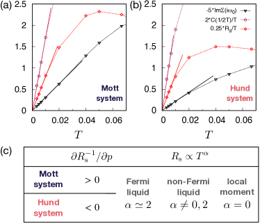
Having established that the sign of is a useful indicator to identify Hund systems, we monitor the temperature dependence of to tell whether a given system at a low temperature follows the FL behavior. In the FL regime at low temperatures, scales as Georges et al. (1996); Werner et al. (2008); Cha et al. (2020); Dumitrescu et al. (2022) and the instantaneous value, , becomes basically -independent. Thus, should concomitantly exhibit the dependence. In contrast, in a local moment regime or a Mott insulator, is -independent. To illustrate this argument, we look at the dependence of divided by () presented in Figs. 3(a–b) for both Mott and Hund systems. We also look at the imaginary part of the local self-energy at the lowest Matsubara frequency, , which exhibits -linear scaling in the FL regime as demonstrated in Ref. Chubukov and Maslov (2012).
We find from Figs. 3(a–b) that both Mott and Hund systems exhibit the FL behavior, namely Chubukov and Maslov (2012), at low temperatures. Interestingly, indeed, and (or, equivalently ) below which the FL behavior sets in. We note that, a Hund metal, if one defines this state as a non-FL, can be identified as a Hund system () lying in a regime in which the exponent of is close to neither 0 nor 2. A summary of our analysis so far is presented in Fig. 3(c).
III.4 Relations of to other quantities: the quasiparticle weight and the spin-orbital separation
Since (: the quasiparticle weight or the inverse of the quasiparticle-mass enhancement within DMFT) Stadler et al. (2019), the behavior of should follow in degenerate-orbital systems. Indeed, the boundary determined by below the FL coherence temperature is almost the same as that determined by at intermediate temperatures as presented in Fig. 4(a). Note also that corresponds to the inverse of the mass enhancement ( is the noninteracting band mass) within the DMFT.
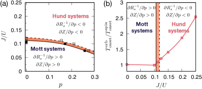
We now compare the Mott–Hund boundary based on the signs of and with that obtained by the onset temperatures of screening of orbital and spin degrees of freedom. These two temperatures, namely for orbital and for spin, are defined as the temperatures below which the Curie law of local moments starts to get violated and Kondo screening sets in Deng et al. (2019). Strong Hund physics in (nearly) degenerate-orbital models at is captured by the separation of these two temperatures, namely Deng et al. (2019); Stadler et al. (2019, 2021); Ryee et al. (2021). With this idea in mind, we here monitor the ratio as a function of for a two-degenerate-orbital () model at and . Specifically, we first evaluate the local orbital/spin susceptibilities: , where for orbital and for spin. Then, we estimate for each value by fitting the high- data to the following formula: . Our result is presented in Fig. 4(b).
Interestingly, we find that the boundary based on the signs of and is in good agreement with that by [Fig. 4(b)]. We can understand it by investigating the Kondo couplings. In the regime of , because . Here, refers to the Kondo couplings when . In this case, the relation (: Kondo coupling for orbital) holds under renormalization group flow, whereby as discussed in Ref. Ryee et al. (2021). Notably, since here, Hund fluctuations which give rise to and are largely masked by non-Hund fluctuations which favor and . Thus, for degenerate-orbital models at , we obtain and for the same range in which . Note, however, that the applicability of our criterion based on the sign of is not limited to degenerate-orbital models at integer fillings. Thus, the criterion is particularly useful in situations where multiple partially-filled orbitals are non-degenerate.
IV Proof of a concept: cuprates and Fe-based superconductors
To corroborate the validity of our proposal, we address two representative Mott and Hund materials. To this end, we solve a two-orbital model ( orbitals; ) for La2CuO4 and a five-orbital model () for LaFeAsO using ab initio parameters. For La2CuO4, we use parameters for a two-orbital model as derived in Ref. Hirayama et al. (2018); see Table 1 and Table S15 in Ref. Hirayama et al. (2018). We take only onsite Coulomb interactions for the model. For LaFeAsO, we use in-plane hopping amplitudes listed in Table IV in Ref. Miyake et al. (2010). For two-body terms, , , and values of , , and eV are adopted for Eq. (1) by parametrizing onsite Coulomb interaction elements listed in Table VIII of Ref. Miyake et al. (2010). We take two-dimensional lattices using in-plane hoppings for both systems and use points in the first Brillouin zone. In their undoped () forms, they both possess electrons. Our main interest is the filling dependence of the inverse of the quasiparticle-mass enhancement and .
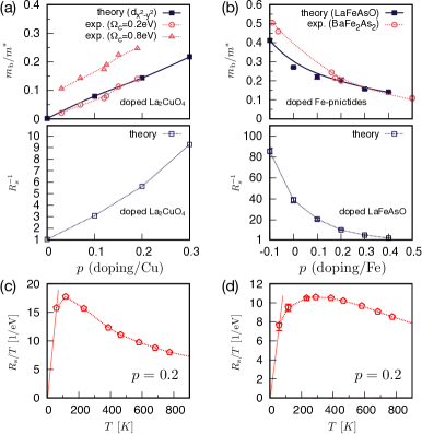
Let us first address the case of La2CuO4 which is a Mott insulator at . Note first that our DMFT calculations using ab initio parameters correctly capture the Mott insulating phase at , namely of vanishes and [Fig. 4(a)]. As increases (increasing hole doping), the correlation strength gets gradually reduced, which is also corroborated by the Drude weights of optical conductivity measurements Lucarelli et al. (2003); Ortolani et al. (2005); Millis et al. (2005) [Fig. 5(a)]. This is the typical behavior of Mott systems. Furthermore, the monotonic increment of both and at least up to implies that Hund physics is not realized in La2CuO4 in this range of electron density. This result is a direct consequence of a sizable between the two orbitals ( Hirayama et al. (2018)), which suppresses significantly the Hund fluctuations by favoring large orbital polarization.
We now turn to the case of FeSCs which have been highlighted over many years as materials realization of Hund metal Georges et al. (2013). While basically the same features are expected for the entire family, we take LaFeAsO for simplicity. The upper panel of Fig. 5(b) presents the calculated from the Sommerfeld coefficient ratio () in comparison with the available experimental data for hole-doped BaFe2As2 Hardy et al. (2010); Popovich et al. (2010); Pramanik et al. (2011); Mu et al. (2009); Kim et al. (2011); Abdel-Hafiez et al. (2012); Storey et al. (2013). Here and are band theory and DMFT (or specific heat) estimates, respectively. Specifically, using a formula: where and , respectively, are the density of states of orbital at the Fermi level obtained from the band theory and the DMFT Kotliar et al. (2006). Note that the formula is strictly valid in a FL regime, so our calculated should not be taken seriously as quantitative estimates.
Both theoretical and experimental displayed in Fig. 5(b) clearly demonstrate that the correlation strength increases with hole doping in FeSCs, which is in sharp contrast to the case of La2CuO4. The doping dependence of further supports the behavior. Based on our scheme, this characteristic feature of , namely , corroborates that FeSCs are governed by strong Hund fluctuations.
Looking at the dependence of [Figs. 5(c–d)], both La2CuO4 and LaFeAsO at -hole doping deviate clearly from the FL behavior (; solid lines are guides for the eye) down to K. Considering that the critical temperature below which the superconductivity emerges is in La0.8Sr0.2CuO4 and in some FeSCs like Ba0.6K0.4Fe2As2 Rotter et al. (2008), the non-FL behavior may be relevant for the emergence of the superconductivity at this doping.
V Possible experimental probes
We now discuss possible experiments to detect , which requires us to measure both short-time () and long-time () local spin-spin correlation functions. Although some subtleties exist, one can resort to x-ray emission or absorption spectroscopy and inelastic neutron scattering (INS). The x-ray techniques can measure the instantaneous local spin moments, , by probing the local fluctuations in the femtosecond scale as discussed in the context of FeSCs Gretarsson et al. (2011, 2013); Pelliciari et al. (2017). INS, on the other hand, can probe the long-time (or low-energy) fluctuations by effectively measuring the imaginary part of the dynamical spin susceptibility, (: crystal-momentum, : real frequency), with the assumption that orbital moments are quenched Toschi et al. (2012); Chen et al. (2020). Using the following relation,
| (4) |
the long-time value can be approximated to the local part of , namely . This is because is the dominant contribution to the -integration when due to a characteristic structure of the kernel in Eq. (4) Randeria et al. (1992). The combination of these two spectroscopies hopefully provides a way to estimate .
If we rely on the quasiparticle weight for the experimental idenfication of Hund correlations instead of using , any probes that can measure the mass enhancement are relevant. As we have already noticed from Figs. 5(a–b), the Drude weight of optical conductivity and the Sommerfeld coefficient of specific heat are standard techniques to estimate , provided is given by the band theory. Furthermore, angle-resolved photoemission spectroscopy (ARPES) enables us to extract the orbital dependent contributions, . Assisted by these experimental techniques, it is feasible to estimate the sign of .
VI Discussion
We finally remark on the related open questions. While our approach based on the sign of should be valid in most of the transition-metal compounds to which the Kanamori (or Slater) type of local interaction [Eq. (1)] is relevant, its applicability to materials with more complicated interactions remains to be resolved. It is also worth investigating the effect of interorbital hopping which plays a crucial role in Mott metal-to-insulator transitions in non-degenerate-orbital systems Kugler and Kotliar (2022); Stepanov (2022); Ryee and Wehling (2023). Nonlocal electron correlations and possible symmetry-breaking transitions affect the low-temperature physics and thus may influence our picture. We expect, however, that measuring should not be hindered by the latter if the measurement is done above the transition temperature. Further studies are required to clarify these issues.
VII Acknowledgments
S.R. is grateful to Tim Wehling for many stimulating conversations. S.R. and M.J.H. were supported by the National Research Foundation of Korea (Grant Nos. 2021R1A2C1009303 and NRF-2018M3D1A1058754). S.R. was also supported by the KAIX Fellowship. S.C. was supported by the U.S. Department of Energy, Office of Science, Basic Energy Sciences as a part of the Computational Materials Science Program. S.C. was also supported by a KIAS individual Grant (No. CG090601) at Korea Institute for Advanced Study. This research used resources of the National Energy Research Scientific Computing Center (NERSC), a U.S. Department of Energy Office of Science User Facility operated under Contract No. DE-AC02-05CH11231.
Appendix A and for a two-degenerate-orbital model on a Bethe lattice
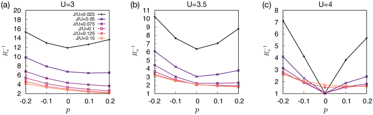
Figure 6 displays additional data for vs. and vs. at three different values of . Here, where is the local self-energy on the imaginary frequency axis; see, e.g., Fig. 6(b). We fitted a fourth-order polynomial to the self-energies in the lowest six imaginary frequency points, following Refs. Mravlje et al. (2011); Ryee et al. (2021).
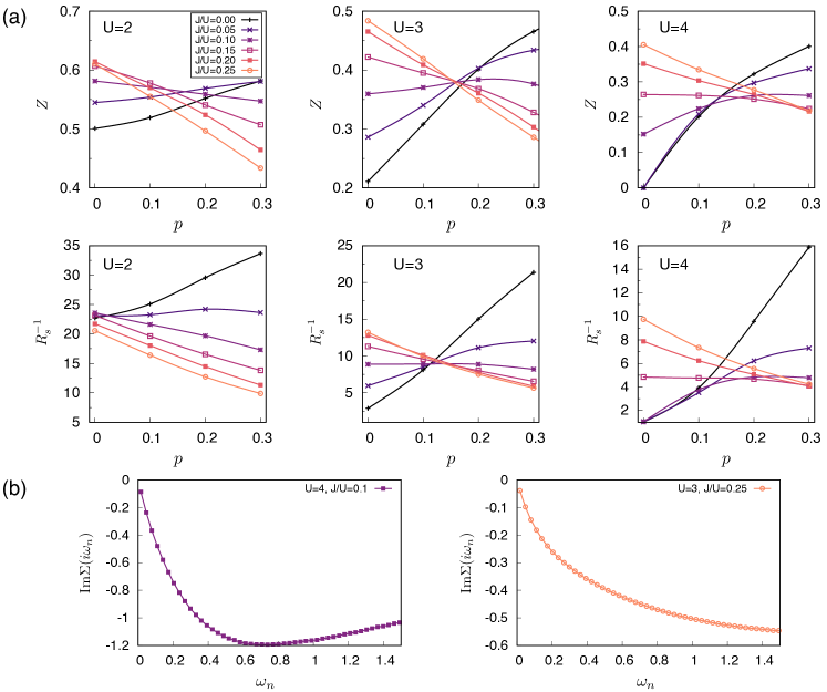
One can notice from Fig. 6 that the value of above which and increases as is increased; the Mott behavior becomes predominant even up to a fairly large value of . Thus, the effect of gets weakened as is increased. A rationale behind this phenomenon can be drawn from the generic form of Kondo couplings obtained via the Schrieffer-Wolff transformation of multiorbital impurity models, which read [Eqs. (17)–(19)]. Thus, at a regime of , by which the effect of Hund coupling on s becomes largely suppressed.
Appendix B and for a two-degenerate-orbital model on a square lattice
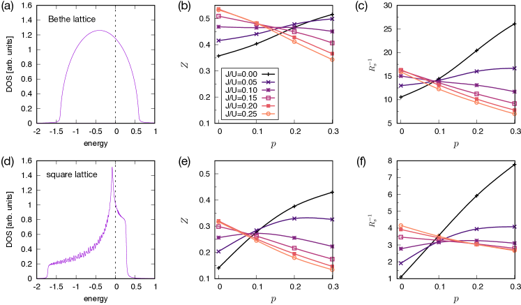
In the main text, we mainly focus on an infinite-dimensional Bethe lattice with semielliptical density of states (DOS) in order to focus on generic features rather than material specific ones. In realistic lattices such as a square lattice, a van Hove singularity (vHS) can exist near the Fermi level. This singularity features a divergence in the DOS [Fig. 7(d)], largely affecting the strength of electron correlations by effectively suppressing low-energy hopping processes; see, e.g., Refs Mravlje et al. (2011); Karp et al. (2020); Lee et al. (2020, 2021) for related discussions. Thus, one may ask whether this vHS has any effects on the signs of and .
Figure 7 presents and as a function of for a square lattice with nearest-neighbor (NN) and next-nearest-neighbor (NNN) hopping amplitudes, and , respectively. Namely, the kinetic part of our Hamiltonian for the square lattice reads , where and denotes, respectively, the NN and NNN sites. Here, and . The results of the Bethe lattice are also plotted for comparison. While the correlation strength itself is enhanced in the square lattice rather than in the Bethe lattice due to the presence of the vHS near the Fermi level, qualitatively the similar behavior is observed for both and : and change their signs from plus to minus by or by .
Appendix C for a three-degenerate-orbital model on a Bethe lattice
A three-degenerate-orbital model has served as a prototypical system for Hund metal physics de’ Medici et al. (2011); Georges et al. (2013). Here, unlike the cases of two-degenerate-orbital models, lifts degeneracy of the ground state atomic multiplets even when , whereby strongly enhances the correlation strength by forming a large composite spin moment Nevidomskyy and Coleman (2009); de’ Medici et al. (2011); Georges et al. (2013). As can be clearly seen from Fig. 8, the overall shape of gradually changes from “V-shape” to a monotonic behavior as increases.
At any rate, for the side, changes its sign by as is discussed for two-orbital models; see Fig. 8. Note here that very low- calculations are required to reach the coherence temperature below which the long-lived quasiparticles are formed in three-orbital models Georges et al. (2013); Kowalski et al. (2019), which is computationally demanding for our DMFT calculations adopting a continuous-time quantum Monte Carlo algorithm. Hence, may not be a good measure of the correlation strength even for the lowest temperature practically accessible within our computation scheme. We thus present only in Fig. 8.
Appendix D Kondo couplings from the Schrieffer-Wolff transformation
Here, we derive Kondo couplings by applying the canonical SW transformation to a relevant impurity model. We follow the strategy depicted in Refs. Yin et al. (2012); Aron and Kotliar (2015); Horvat et al. (2016).
Note first that the original lattice model is mapped onto an auxiliary impurity model in DMFT. Let us thus write down the impurity Hamiltonian with symmetry:
| (5) |
where
| (6) | ||||
| (7) | ||||
| (8) |
Here, () is the creation (destruction) operator for bath states. . We will later get back to the form of Eq. (1) which includes the pair-hopping term and for .
Our goal is, by integrating out valence fluctuations, to construct an effective Kondo model for low-energy physics:
| (9) |
where is given by the SW transformation:
| (10) |
with being the projector to the atomic ground state multiplet (with eigenvalue ) in charge subspace of Eq. (6). project onto the atomic multiplets of Eq. (6) having eigenvalues of in charge subspaces. The subscript is the index for labeling different multiplets. refers to the charge excitation energy.
Now, we use the following relation which holds for symmetry:
| (11) |
where is the generator of the symmetric group, namely, corresponds to Pauli matrices () for , and to Gell-Mann matrices for . We hereafter use the Einstein summation convention for simplicity. Inserting Eq. (11) into Eq. (10) for both spin and orbital leads to the following form of :
| (12) |
and are the spin and orbital operators for impurity degrees of freedom. , , , and are Kondo couplings for potential scattering, spin, orbital, and spin-orbital terms, which are given by
| (13) | ||||
| (14) | ||||
| (15) | ||||
| (16) |
Here, denotes the atomic ground state multiplet in the charge subspace. Since the first term in Eq. (12) is irrelevant for dynamics of local moments Aron and Kotliar (2015); Horvat et al. (2016), we discard from our discussion.
| Index | Eigenstate | Eigenvalue | |||
| 1 | 0 | 0 | 0 | 0 | |
| 2 | 1 | 1/2 | 1/2 | ||
| 3 | 1 | 1/2 | 1/2 | ||
| 4 | 1 | 1/2 | -1/2 | ||
| 5 | 1 | 1/2 | -1/2 | ||
| 6 | 2 | 1 | 1 | ||
| 7 | 2 | 1 | 0 | ||
| 8 | 2 | 1 | -1 | ||
| 9 | 2 | 0 | 0 | ||
| 10 | 2 | 0 | 0 | ||
| 11 | 2 | 0 | 0 | ||
| 12 | 3 | 1/2 | 1/2 | ||
| 13 | 3 | 1/2 | 1/2 | ||
| 14 | 3 | 1/2 | -1/2 | ||
| 15 | 3 | 1/2 | -1/2 | ||
| 16 | 4 | 0 | 0 |
While the discussion below is valid for any models, let us focus on the case of two orbitals () with . For generic cases, refer to Ref. Aron and Kotliar (2015). Eigenstates and eigenvalues of Eq. (6) are listed in Table 1. We have the freedom to choose , , and to evaluate Eqs. (14)–(16). Hence, for convenience, and . Kondo couplings are now given by:
| (17) | ||||
| (18) | ||||
| (19) |
where the subscript of () refers to the index of the eigenstate in Table 1. In the second equalities of the above equations, we re-write terms using which denotes the excitation energy from the ground state to the excited atomic multiplet . The subscript () refers to the -th lowest eigenvalue in the corresponding subspace. We henceforth restrict ourselves to a region where and .
| Index | Eigenstate | Eigenvalue | |||
| 1 | 0 | 0 | 0 | 0 | |
| 2 | 1 | 1/2 | 1/2 | ||
| 3 | 1 | 1/2 | 1/2 | ||
| 4 | 1 | 1/2 | -1/2 | ||
| 5 | 1 | 1/2 | -1/2 | ||
| 6 | 2 | 1 | 1 | ||
| 7 | 2 | 1 | 0 | ||
| 8 | 2 | 1 | -1 | ||
| 9 | 2 | 0 | 0 | ||
| 10 | 2 | 0 | 0 | ||
| 11 | 2 | 0 | 0 | ||
| 12 | 3 | 1/2 | 1/2 | ||
| 13 | 3 | 1/2 | 1/2 | ||
| 14 | 3 | 1/2 | -1/2 | ||
| 15 | 3 | 1/2 | -1/2 | ||
| 16 | 4 | 0 | 0 |
We now consider responses of these couplings due to changes in filling. To mimic the effect of a small increase in , let us consider a situation where is slightly decreased by (), i.e., . The concomitant changes in s are given by:
| (20) | ||||
| (21) | ||||
| (22) |
When , is equal to . Since is larger than for the hole doped side, Eqs. (20)–(22) are all positive implying that all the Kondo coupling constants evolve in a way to weaken the correlation strength. When and , on the other hand, is smaller than the other s. In this case, Eqs. (20)–(22) are controlled mainly by the terms related to . Thus, we arrive at the following relations for :
| (23) | ||||
| (24) | ||||
| (25) |
The above relations indicate that only decreases due to Hund fluctuations as is increased. In contrast, increases with , favoring the screening of orbital degrees of freedom, which is consistent with the enhanced spin-orbital separation by for a finite in three-orbital models Horvat et al. (2016); Stadler et al. (2019).
| Index | Eigenstate | Eigenvalue | |||
| 1 | 0 | 0 | 0 | 0 | |
| 2 | 1 | 1/2 | 1/2 | ||
| 3 | 1 | 1/2 | 1/2 | ||
| 4 | 1 | 1/2 | -1/2 | ||
| 5 | 1 | 1/2 | -1/2 | ||
| 6 | 2 | 1 | 1 | ||
| 7 | 2 | 1 | 0 | ||
| 8 | 2 | 1 | -1 | ||
| 9 | 2 | 0 | 0 | ||
| 10 | 2 | 0 | 0 | ||
| 11 | 2 | 0 | 0 | ||
| 12 | 3 | 1/2 | 1/2 | ||
| 13 | 3 | 1/2 | 1/2 | ||
| 14 | 3 | 1/2 | -1/2 | ||
| 15 | 3 | 1/2 | -1/2 | ||
| 16 | 4 | 0 | 0 |
Having evidenced that the sign of is influenced by , we now consider Eq. (1) with for . In this case, only symmetry of spin is retained. Using eigenstates and eigenvalues listed in Table 2 and Table 3, we get the following relations for :
| (26) | ||||
| (27) |
where and . Applying the same procedure used for getting Eq. (23) for results in
| (28) | ||||
| (29) |
Finally, we briefly discuss the case of and with Eq. (1) being . We set and . Using eigenstates and eigenvalues listed in Table 2 and Table 3, we arrive at
| (30) | ||||
| (31) |
where () in this case denotes the excitation energy from to the excited atomic multiplet . The change of under is given by
| (32) | ||||
| (33) |
As for , Eqs. (32–33) are always positive. Note that irrespective of and for , which is in sharp contrast to the case of .
Appendix E and as a function of for two-orbital models on a Bethe lattice
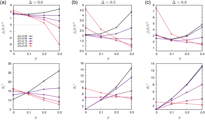
Figure 9 displays and as a function of for two-orbital models on a Bethe lattice with . Although is a bare Kondo coupling which will be scaled via renormalization group flow, the behavior of as a function of is qualitatively consistent with that of .
Appendix F and its relation to for the cases of and
Our criterion based on the sign of cannot distinguish Mott and Hund correlations for the negative () and very large of ( is an arbitrarily small positive number) by which the system is close to half-filling. To understand these cases, let us focus on a two-degenerate-orbital model with in Eq. (6).
F.1 The case of .
This case is exactly the same as the “electron doping” () to a system of electron filling. For this filling, Kondo coupling for the spin degree of freedom, , is given by Eq. (17). We now consider response of due to electron doping . To mimic the effect of a small increase in , let us consider a situation where is slightly increased by (), i.e., . As a consequence, . Thus, the concomitant change in is given by:
| (34) |
When , is equal to . Furthermore, since is smaller than for the electron doped side, Eq. (34) is positive. This means that Kondo screening for spin becomes more effective by electron doping, and thereby correlation strength is reduced. Thus, . This conclusion is actually consistent with our physical intuition that Mott physics is weakened by doping an integer-filled system.
When is large, is much smaller than . This observation leads us to the following expression.
| (35) |
As in the case of , also increases by electron doping. Thus, we expect even for the case of large .
To conclude our discussion on the case of , we can confirm from the analysis of that spin screening becomes more effective upon doping no matter how large is. Physically, this is because the case of (or, equivalently electron filling of ) is the doping by which the “Hund fluctuations” (ferromagnetic charge fluctuations between the dominant atomic multiplets and higher-spin ones in a neighboring charge subspace, i.e., the term containing ) are weakened. Thus, our criterion based on the sign of is not applicable to this case.
F.2 The case of ( is an arbitrarily small positive number).
This case is exactly the same as the “electron doping” () to a system of electron filling (half filling). Kondo coupling for spin is given by Eq. (30). To mimic the effect of a small increase in , let us consider a situation where is slightly increased by (), i.e., . As a consequence, . Thus, the concomitant change in is given by:
| (36) |
Since on the electron doped side, Eq. (36) is always positive irrespective of . This is because the role of doping in this case is to reduce the weight of the high-spin multiplet, namely which is responsible for realizing Hund metal physics. Our criterion measures how large the effect of the high-spin “half-filled” multiplet (i.e., for ) is on the low-energy physics while the system is far away from half fillng. Since already dominates the atomic states, it is not surprising at all that our proposal is inapplicable to this case.
References
- Imada et al. (1998) Masatoshi Imada, Atsushi Fujimori, and Yoshinori Tokura, “Metal-insulator transitions,” Rev. Mod. Phys. 70, 1039–1263 (1998).
- Lee et al. (2006) Patrick A. Lee, Naoto Nagaosa, and Xiao-Gang Wen, “Doping a mott insulator: Physics of high-temperature superconductivity,” Rev. Mod. Phys. 78, 17–85 (2006).
- Norman et al. (2005) M. R. Norman, D. Pines, and C. Kallin, “The pseudogap: friend or foe of high ?” Advances in Physics 54, 715–733 (2005).
- Keimer et al. (2015) B. Keimer, S. A. Kivelson, M. R. Norman, S. Uchida, and J. Zaanen, “From quantum matter to high-temperature superconductivity in copper oxides,” Nature 518, 179–186 (2015).
- Haule and Kotliar (2009) K Haule and G Kotliar, “Coherence–incoherence crossover in the normal state of iron oxypnictides and importance of ’s rule coupling,” New Journal of Physics 11, 025021 – 025033 (2009).
- Mravlje et al. (2011) Jernej Mravlje, Markus Aichhorn, Takashi Miyake, Kristjan Haule, Gabriel Kotliar, and Antoine Georges, “Coherence-incoherence crossover and the mass-renormalization puzzles in ,” Phys. Rev. Lett. 106, 096401 – 096404 (2011).
- Werner et al. (2012) Philipp Werner, Michele Casula, Takashi Miyake, Ferdi Aryasetiawan, Andrew J. Millis, and Silke Biermann, “Satellites and large doping and temperature dependence of electronic properties in hole-doped BaFe2As2,” Nature Physics 8, 331–337 (2012).
- Werner et al. (2008) Philipp Werner, Emanuel Gull, Matthias Troyer, and Andrew J. Millis, “Spin freezing transition and non--liquid self-energy in a three-orbital model,” Phys. Rev. Lett. 101, 166405 – 166408 (2008).
- Nevidomskyy and Coleman (2009) Andriy H. Nevidomskyy and P. Coleman, “Kondo resonance narrowing in - and -electron systems,” Phys. Rev. Lett. 103, 147205 (2009).
- de’ Medici (2011) Luca de’ Medici, “Hund’s coupling and its key role in tuning multiorbital correlations,” Phys. Rev. B 83, 205112 – 205122 (2011).
- de’ Medici et al. (2011) Luca de’ Medici, Jernej Mravlje, and Antoine Georges, “Janus-faced influence of und’s rule coupling in strongly correlated materials,” Phys. Rev. Lett. 107, 256401 – 256404 (2011).
- Yin et al. (2011) Z. P. Yin, K. Haule, and G. Kotliar, “Kinetic frustration and the nature of the magnetic and paramagnetic states in iron pnictides and iron chalcogenides,” Nature Materials 10, 932–935 (2011).
- Yin et al. (2012) Z. P. Yin, K. Haule, and G. Kotliar, “Fractional power-law behavior and its origin in iron-chalcogenide and ruthenate superconductors: Insights from first-principles calculations,” Phys. Rev. B 86, 195141 – 195149 (2012).
- Toschi et al. (2012) A. Toschi, R. Arita, P. Hansmann, G. Sangiovanni, and K. Held, “Quantum dynamical screening of the local magnetic moment in Fe-based superconductors,” Phys. Rev. B 86, 064411 (2012).
- Georges et al. (2013) Antoine Georges, Luca de’ Medici, and Jernej Mravlje, “Strong correlations from Hund’s coupling,” Annual Review of Condensed Matter Physics 4, 137–178 (2013).
- de’ Medici et al. (2014) Luca de’ Medici, Gianluca Giovannetti, and Massimo Capone, “Selective physics as a key to iron superconductors,” Phys. Rev. Lett. 112, 177001 – 177005 (2014).
- Khajetoorians et al. (2015) A. A. Khajetoorians, M. Valentyuk, M. Steinbrecher, T. Schlenk, A. Shick, J. Kolorenc, A. I. Lichtenstein, T. O. Wehling, R. Wiesendanger, and J. Wiebe, “Tuning emergent magnetism in a Hund’s impurity,” Nature Nanotechnology 10, 958–964 (2015).
- Fanfarillo and Bascones (2015) L. Fanfarillo and E. Bascones, “Electronic correlations in metals,” Phys. Rev. B 92, 075136 – 075142 (2015).
- Hoshino and Werner (2015) Shintaro Hoshino and Philipp Werner, “Superconductivity from emerging magnetic moments,” Phys. Rev. Lett. 115, 247001 – 247005 (2015).
- Aron and Kotliar (2015) Camille Aron and Gabriel Kotliar, “Analytic theory of ’s metals: a renormalization group perspective,” Phys. Rev. B 91, 041110 – 041114 (2015).
- Stadler et al. (2015) K. M. Stadler, Z. P. Yin, J. von Delft, G. Kotliar, and A. Weichselbaum, “Dynamical mean-field theory plus numerical renormalization-group study of spin-orbital separation in a three-band metal,” Phys. Rev. Lett. 115, 136401 – 136405 (2015).
- Horvat et al. (2016) Alen Horvat, Rok Žitko, and Jernej Mravlje, “Low-energy physics of three-orbital impurity model with interaction,” Phys. Rev. B 94, 165140 – 165150 (2016).
- Stadler et al. (2019) K.M. Stadler, G. Kotliar, A. Weichselbaum, and J. von Delft, “ versus in a three-band – model: on the origin of strong correlations in metals,” Annals of Physics 405, 365 – 409 (2019).
- Deng et al. (2019) Xiaoyu Deng, Katharina M. Stadler, Kristjan Haule, Andreas Weichselbaum, Jan von Delft, and Gabriel Kotliar, “Signatures of Mottness and Hundness in archetypal correlated metals,” Nature Communications 10, 2721 (2019).
- Isidori et al. (2019) Aldo Isidori, Maja Berović, Laura Fanfarillo, Luca de’ Medici, Michele Fabrizio, and Massimo Capone, “Charge disproportionation, mixed valence, and effect in multiorbital systems: A tale of two insulators,” Phys. Rev. Lett. 122, 186401 – 186406 (2019).
- Ryee et al. (2020) Siheon Ryee, Patrick Sémon, Myung Joon Han, and Sangkook Choi, “Nonlocal Coulomb interaction and spin-freezing crossover as a route to valence-skipping charge order,” npj Quantum Materials 5, 19 (2020).
- Huang and Lu (2020) Li Huang and Haiyan Lu, “Signatures of Hundness in kagome metals,” Phys. Rev. B 102, 125130 (2020).
- Chen et al. (2020) Xiang Chen, Igor Krivenko, Matthew B. Stone, Alexander I. Kolesnikov, Thomas Wolf, Dmitry Reznik, Kevin S. Bedell, Frank Lechermann, and Stephen D. Wilson, “Unconventional Hund metal in a weak itinerant ferromagnet,” Nature Communications 11, 3076 (2020).
- Lee et al. (2020) Hyeong Jun Lee, Choong H. Kim, and Ara Go, “Interplay between spin-orbit coupling and van Hove singularity in the Hund’s metallicity of ,” Phys. Rev. B 102, 195115 (2020).
- Wang et al. (2020) Y. Wang, C.-J. Kang, H. Miao, and G. Kotliar, “Hund’s metal physics: From to ,” Phys. Rev. B 102, 161118 (2020).
- Watzenböck et al. (2020) C. Watzenböck, M. Edelmann, D. Springer, G. Sangiovanni, and A. Toschi, “Characteristic timescales of the local moment dynamics in Hund’s metals,” Phys. Rev. Lett. 125, 086402 (2020).
- Karp et al. (2020) Jonathan Karp, Max Bramberger, Martin Grundner, Ulrich Schollwöck, Andrew J. Millis, and Manuel Zingl, “ and : Disentangling the roles of Hund’s and van Hove physics,” Phys. Rev. Lett. 125, 166401 (2020).
- Fanfarillo et al. (2020) Laura Fanfarillo, Angelo Valli, and Massimo Capone, “Synergy between Hund-driven correlations and boson-mediated superconductivity,” Phys. Rev. Lett. 125, 177001 (2020).
- Kang et al. (2020) Byungkyun Kang, Corey Melnick, Patrick Semon, Siheon Ryee, Myung Joon Han, Gabriel Kotliar, and Sangkook Choi, “Infinite-layer nickelates as Ni-eg Hund’s metals,” arXiv preprint arXiv:2007.14610 (2020).
- Bramberger et al. (2021) Max Bramberger, Jernej Mravlje, Martin Grundner, Ulrich Schollwöck, and Manuel Zingl, “: A Hund’s metal in the presence of strong spin-orbit coupling,” Phys. Rev. B 103, 165133 (2021).
- Ryee et al. (2021) Siheon Ryee, Myung Joon Han, and Sangkook Choi, “Hund physics landscape of two-orbital systems,” Phys. Rev. Lett. 126, 206401 (2021).
- Drouin-Touchette et al. (2021) Victor Drouin-Touchette, Elio J. König, Yashar Komijani, and Piers Coleman, “Emergent moments in a Hund’s impurity,” Phys. Rev. B 103, 205147 (2021).
- Stadler et al. (2021) K. M. Stadler, G. Kotliar, S.-S. B. Lee, A. Weichselbaum, and J. von Delft, “Differentiating Hund from Mott physics in a three-band Hubbard-Hund model: Temperature dependence of spectral, transport, and thermodynamic properties,” Phys. Rev. B 104, 115107 (2021).
- Lee et al. (2021) Hyeong Jun Lee, Choong H. Kim, and Ara Go, “Hund’s metallicity enhanced by a van Hove singularity in cubic perovskite systems,” Phys. Rev. B 104, 165138 (2021).
- Stepanov et al. (2021) Evgeny A. Stepanov, Yusuke Nomura, Alexander I. Lichtenstein, and Silke Biermann, “Orbital isotropy of magnetic fluctuations in correlated electron materials induced by Hund’s exchange coupling,” Phys. Rev. Lett. 127, 207205 (2021).
- Nomura et al. (2022) Yusuke Nomura, Shiro Sakai, and Ryotaro Arita, “Fermi surface expansion above critical temperature in a Hund ferromagnet,” Phys. Rev. Lett. 128, 206401 (2022).
- Drouin-Touchette et al. (2022) Victor Drouin-Touchette, Elio J. König, Yashar Komijani, and Piers Coleman, “Interplay of charge and spin fluctuations in a Hund’s coupled impurity,” Phys. Rev. Res. 4, L042011 (2022).
- Kim et al. (2022) Taek Jung Kim, Siheon Ryee, and Myung Joon Han, “Fe3GeTe2: a site-differentiated Hund metal,” npj Computational Materials 8, 245 (2022).
- Georges et al. (1996) Antoine Georges, Gabriel Kotliar, Werner Krauth, and Marcelo J. Rozenberg, “Dynamical mean-field theory of strongly correlated fermion systems and the limit of infinite dimensions,” Rev. Mod. Phys. 68, 13–125 (1996).
- Kotliar et al. (2006) G. Kotliar, S. Y. Savrasov, K. Haule, V. S. Oudovenko, O. Parcollet, and C. A. Marianetti, “Electronic structure calculations with dynamical mean-field theory,” Rev. Mod. Phys. 78, 865–951 (2006).
- Gull et al. (2011) Emanuel Gull, Andrew J. Millis, Alexander I. Lichtenstein, Alexey N. Rubtsov, Matthias Troyer, and Philipp Werner, “Continuous-time methods for quantum impurity models,” Rev. Mod. Phys. 83, 349 – 404 (2011).
- Choi et al. (2019) Sangkook Choi, Patrick Semon, Byungkyun Kang, Andrey Kutepov, and Gabriel Kotliar, “ComDMFT: A massively parallel computer package for the electronic structure of correlated-electron systems,” Computer Physics Communications 244, 277–294 (2019).
- Kowalski et al. (2019) Alexander Kowalski, Andreas Hausoel, Markus Wallerberger, Patrik Gunacker, and Giorgio Sangiovanni, “State and superstate sampling in hybridization-expansion continuous-time quantum monte carlo,” Phys. Rev. B 99, 155112 (2019).
- Schrieffer and Wolff (1966) J. R. Schrieffer and P. A. Wolff, “Relation between the Anderson and Kondo Hamiltonians,” Phys. Rev. 149, 491–492 (1966).
- Cha et al. (2020) Peter Cha, Nils Wentzell, Olivier Parcollet, Antoine Georges, and Eun-Ah Kim, “Linear resistivity and Sachdev-Ye-Kitaev (SYK) spin liquid behavior in a quantum critical metal with spin-1/2 fermions,” Proceedings of the National Academy of Sciences 117, 18341–18346 (2020).
- Dumitrescu et al. (2022) Philipp T. Dumitrescu, Nils Wentzell, Antoine Georges, and Olivier Parcollet, “Planckian metal at a doping-induced quantum critical point,” Phys. Rev. B 105, L180404 (2022).
- Chubukov and Maslov (2012) Andrey V. Chubukov and Dmitrii L. Maslov, “First-matsubara-frequency rule in a Fermi liquid. i. fermionic self-energy,” Phys. Rev. B 86, 155136 (2012).
- Hirayama et al. (2018) Motoaki Hirayama, Youhei Yamaji, Takahiro Misawa, and Masatoshi Imada, “Ab initio effective hamiltonians for cuprate superconductors,” Phys. Rev. B 98, 134501 (2018).
- Miyake et al. (2010) Takashi Miyake, Kazuma Nakamura, Ryotaro Arita, and Masatoshi Imada, “Comparison of ab initio low-energy models for LaFePO, LaFeAsO, BaFe2As2, LiFeAs, FeSe, and FeTe: Electron correlation and covalency,” Journal of the Physical Society of Japan 79, 044705 (2010).
- Lucarelli et al. (2003) A. Lucarelli, S. Lupi, M. Ortolani, P. Calvani, P. Maselli, M. Capizzi, P. Giura, H. Eisaki, N. Kikugawa, T. Fujita, M. Fujita, and K. Yamada, “Phase diagram of probed in the infared: Imprints of charge stripe excitations,” Phys. Rev. Lett. 90, 037002 (2003).
- Ortolani et al. (2005) M. Ortolani, P. Calvani, and S. Lupi, “Frequency-dependent thermal response of the charge system and the restricted sum rules of ,” Phys. Rev. Lett. 94, 067002 (2005).
- Millis et al. (2005) A. J. Millis, A. Zimmers, R. P. S. M. Lobo, N. Bontemps, and C. C. Homes, “Mott physics and the optical conductivity of electron-doped cuprates,” Phys. Rev. B 72, 224517 (2005).
- Hardy et al. (2010) F. Hardy, P. Burger, T. Wolf, R. A. Fisher, P. Schweiss, P. Adelmann, R. Heid, R. Fromknecht, R. Eder, D. Ernst, H. v. Löhneysen, and C. Meingast, “Doping evolution of superconducting gaps and electronic densities of states in Ba(Fe1-xCox)2As2 iron pnictides,” EPL (Europhysics Letters) 91, 47008 (2010).
- Popovich et al. (2010) P. Popovich, A. V. Boris, O. V. Dolgov, A. A. Golubov, D. L. Sun, C. T. Lin, R. K. Kremer, and B. Keimer, “Specific heat measurements of single crystals: Evidence for a multiband strong-coupling superconducting state,” Phys. Rev. Lett. 105, 027003 (2010).
- Pramanik et al. (2011) A. K. Pramanik, M. Abdel-Hafiez, S. Aswartham, A. U. B. Wolter, S. Wurmehl, V. Kataev, and B. Büchner, “Multigap superconductivity in single crystals of Ba0.65Na0.35Fe2As2: A calorimetric investigation,” Phys. Rev. B 84, 064525 (2011).
- Mu et al. (2009) Gang Mu, Huiqian Luo, Zhaosheng Wang, Lei Shan, Cong Ren, and Hai-Hu Wen, “Low temperature specific heat of the hole-doped single crystals,” Phys. Rev. B 79, 174501 (2009).
- Kim et al. (2011) J. S. Kim, E. G. Kim, G. R. Stewart, X. H. Chen, and X. F. Wang, “Specific heat in KFe2As2 in zero and applied magnetic field,” Phys. Rev. B 83, 172502 (2011).
- Abdel-Hafiez et al. (2012) M. Abdel-Hafiez, S. Aswartham, S. Wurmehl, V. Grinenko, C. Hess, S.-L. Drechsler, S. Johnston, A. U. B. Wolter, B. Büchner, H. Rosner, and L. Boeri, “Specific heat and upper critical fields in KFe2As2 single crystals,” Phys. Rev. B 85, 134533 (2012).
- Storey et al. (2013) J. G. Storey, J. W. Loram, J. R. Cooper, Z. Bukowski, and J. Karpinski, “Electronic specific heat of Ba1-xKxFe2As2 from 2 to 380 k,” Phys. Rev. B 88, 144502 (2013).
- Rotter et al. (2008) Marianne Rotter, Marcus Tegel, and Dirk Johrendt, “Superconductivity at 38 k in the iron arsenide ,” Phys. Rev. Lett. 101, 107006 (2008).
- Gretarsson et al. (2011) H. Gretarsson, A. Lupascu, Jungho Kim, D. Casa, T. Gog, W. Wu, S. R. Julian, Z. J. Xu, J. S. Wen, G. D. Gu, R. H. Yuan, Z. G. Chen, N.-L. Wang, S. Khim, K. H. Kim, M. Ishikado, I. Jarrige, S. Shamoto, J.-H. Chu, I. R. Fisher, and Young-June Kim, “Revealing the dual nature of magnetism in iron pnictides and iron chalcogenides using x-ray emission spectroscopy,” Phys. Rev. B 84, 100509 (2011).
- Gretarsson et al. (2013) H. Gretarsson, S. R. Saha, T. Drye, J. Paglione, Jungho Kim, D. Casa, T. Gog, W. Wu, S. R. Julian, and Young-June Kim, “Spin-state transition in the Fe pnictides,” Phys. Rev. Lett. 110, 047003 (2013).
- Pelliciari et al. (2017) Jonathan Pelliciari, Yaobo Huang, Kenji Ishii, Chenglin Zhang, Pengcheng Dai, Gen Fu Chen, Lingyi Xing, Xiancheng Wang, Changqing Jin, Hong Ding, Philipp Werner, and Thorsten Schmitt, “Magnetic moment evolution and spin freezing in doped BaFe2As2,” Scientific Reports 7, 8003 (2017).
- Randeria et al. (1992) Mohit Randeria, Nandini Trivedi, Adriana Moreo, and Richard T. Scalettar, “Pairing and spin gap in the normal state of short coherence length superconductors,” Phys. Rev. Lett. 69, 2001–2004 (1992).
- Kugler and Kotliar (2022) Fabian B. Kugler and Gabriel Kotliar, “Is the orbital-selective Mott phase stable against interorbital hopping?” Phys. Rev. Lett. 129, 096403 (2022).
- Stepanov (2022) Evgeny A. Stepanov, “Eliminating orbital selectivity from the metal-insulator transition by strong magnetic fluctuations,” Phys. Rev. Lett. 129, 096404 (2022).
- Ryee and Wehling (2023) Siheon Ryee and Tim O. Wehling, “Switching between Mott-Hubbard and Hund physics in Moiré Quantum Simulators,” Nano Letters 23, 573–579 (2023).