Log Barriers for Safe Black-box Optimization with Application to Safe Reinforcement Learning

Abstract

Optimizing noisy functions online, when evaluating the objective requires experiments on a deployed system, is a crucial task arising in manufacturing, robotics and many others. Often, constraints on safe inputs are unknown ahead of time, and we only obtain noisy information, indicating how close we are to violating the constraints. Yet, safety must be guaranteed at all times, not only for the final output of the algorithm.

We introduce a general approach for seeking a stationary point in high dimensional non-linear stochastic optimization problems in which maintaining safety during learning is crucial. Our approach called LB-SGD is based on applying stochastic gradient descent (SGD) with a carefully chosen adaptive step size to a logarithmic barrier approximation of the original problem. We provide a complete convergence analysis of non-convex, convex, and strongly-convex smooth constrained problems, with first-order and zeroth-order feedback. Our approach yields efficient updates and scales better with dimensionality compared to existing approaches.

We empirically compare the sample complexity and the computational cost of our method with existing safe learning approaches. Beyond synthetic benchmarks, we demonstrate the effectiveness of our approach on minimizing constraint violation in policy search tasks in safe reinforcement learning (RL).

Keywords: Stochastic optimization, safe learning, black-box optimization, smooth constrained optimization, reinforcement learning.

1 Introduction

Many optimization tasks in robotics, manufacturing, health sciences, and finance require minimizing a loss function under constraints and uncertainties. In several applications, these constraints are unknown at the outset of optimization, and one can infer the feasibility of inputs only from noisy measurements. For example, in manufacturing, the learner may want to tune the parameters of a machine. However, they can only observe noisy measurements of the constraints. Alternatively, in learning-based control tasks, e.g., in robotics, one may want to iteratively collect measurements and improve a pre-trained control policy in new environments. In such cases, during the optimization process, it is crucial to only query points (decision vectors) that satisfy the safety constraints, i.e., lie inside the feasible set, since querying infeasible points could lead to harmful consequences (Kirschner et al., 2019; Berkenkamp et al., 2016b). In such settings, even if the state constraints are known in advance, the learner may only have an approximate model of the true dynamics, e.g., through a simulator or a learned model. This implies that in the control policy space, exact constraints are also unknown, which makes non-violation of safety constraints while learning a challenging and important task. In the manufacturing example, one wants to sequentially update the parameters and take measurements of the machine performance while not violating the temperature limit during the learning not to break the machine. In the robotics example, while learning the new policy in the new environment, one wants to perform only safe policy updates, avoiding dangerous situations on the road. This problem is known as safe learning.

In this work, we consider two general settings of safe learning. In the first case, we can only access the objective and constraints from noisy value measurements. This is referred to the zeroth-order (black-box) noisy information setting. In the second case, noisy gradient measurements are also available. This is referred to as the first-order noisy information setting.

The literature on safe learning has focused mainly on the black-box setting. To compare various methods in this setting, we can estimate their sample and computational complexity. The sample complexity represents the number of oracle queries in total that the learner has to make during the optimization to achieve the specific final accuracy $\varepsilon>0$. Computational complexity is the total number of arithmetical operations the algorithm requires to achieve accuracy $\varepsilon$.

In the safe learning case, a large body of work is based on safe Bayesian optimization (BO) (Sui et al., 2015a; Berkenkamp et al., 2020). These approaches are typically based upon fitting a Gaussian process (GP) as a surrogate of the unknown objective and constraints functions based on the collected measurements. GPs are built using the predefined kernel function.

Although safe BO algorithms are provably safe and globally optimal, without simplifying assumptions, BO methods suffer from the curse of dimensionality (Frazier, 2018; Moriconi et al., 2019; Eriksson and Jankowiak, 2021). That is, their sample complexity might depend exponentially on the dimensionality for most commonly used kernels, including the squared exponential kernel (Srinivas et al., 2012). Moreover, their computational cost can also scale exponentially on the dimensionality since BO methods have to solve a non-linear programming (NLP) sub-problem at each iteration, which is, in general, an NP-hard problem. Together with this challenge, their computational cost scales cubically with the number of measurements, which provides a significant additional restriction on the number of measurements. These challenges make BO methods harder to employ on medium-to-big scale problems.

Thus, our primary motivation is to find an algorithm such that 1) its computational complexity scales efficiently to a large number of data points; 2) its sample complexity scales efficiently to high dimensions; and 3) it keeps optimization iterates within the feasible set of parameters with high probability.

We propose Log Barriers SGD (LB-SGD), an algorithm that addresses the safe learning task by minimizing the log barrier approximation of the problem. This minimization is done by using Stochastic Gradient Descent (SGD) with a carefully chosen adaptive step size. We prove safety and derive the convergence rate of the algorithm for the convex and non-convex case (to the stationary point) and demonstrate LB-SGD’s performance compared to other safe BO optimization algorithms on a series of experiments with various scales.

Our contributions

We summarize our contributions below:

• We propose a unified approach for safe learning given a zeroth-order or first-order stochastic oracle. We prove that our approach generates feasible iterations with high probability and converges to a stationary point. Each iteration of the proposed method is computationally cheap and does not require solving any subproblems.

• In contrast to our past work on the log barrier approach (Usmanova et al., 2020), we develop a less conservative adaptive step size based on the smoothness constant instead of the Lipschitz constant of the constraints, enabling a tighter analysis.

• We provide a unified analysis, deriving the convergence rate of our algorithm for the stochastic non-convex, convex, and strongly-convex problems. We establish convergence despite the non-smoothness of the log barrier and the increasingly high variance of the log barrier gradient estimator.

• We empirically demonstrate that our method can scale to problems with high dimensions, in which previous methods fail. Moreover, we show the effectiveness of our approach in minimizing constraint violation in policy search in a high-dimensional constrained reinforcement learning (RL) problem.

Related work

Although first-order stochastic optimization is widely explored (Nemirovsky and Yudin, 1985; Juditsky et al., 2013; Lan, 2020), we are not aware of any work addressing safe learning for first-order stochastic optimization. Therefore, even though our work also covers the first-order information case, we focus our review on the zeroth-order (black-box) optimization. Most relevant to our work are two areas: 1) feasible optimization approaches addressing smooth problems with known constraints; 2) existing safe approaches addressing smooth unknown objectives and constraints (including linear constraints). Here, by unknown constraints, we mean that we only have access to a noisy zeroth-order oracle of the constraints while solving the constrained optimization problem. By feasible optimization approaches, we refer to constrained optimization methods that generate a feasible optimization trajectory. For example, the Projected Gradient Descent and Frank-Wolfe are feasible, whereas dual approaches such as Augmented Lagrangian are infeasible.

There also exists another large body of work addressing probabilistic or chance constraints (Shapiro et al., 2009). This line of work aims to solve an optimization problem with probabilistic constraints in the form $\mathbb{P}\{F^{i}(x,\xi)\leq 0\}\geq 1-\delta.$ However, the main difference is that in our safe learning task, we aim to satisfy the uncertain constraints with high probability during the learning process, not only in the end. Another issue is that the chance constraints problem, in general, is also a complex task with no universal solution. Typically, to address it, one requires either a significant number of (unsafe) measurements (e.g., in the scenario approach) or assumes some knowledge about the structure of the constraints a priori (e.g., in robust optimization). In contrast, in the current work, we propose a way to address the safe learning task without prior knowledge of the structure of the constraints.

We summarize the discussion of the algorithms from the past work as well as the best known lower bounds in Table 1. All works in Table 1 consider one-point feedback, except for Balasubramanian and Ghadimi (2018) who consider two-point feedback. Two-point feedback allows access to the function measurements with the same noise disturbance in at least two different points, whereas one-point feedback cannot guarantee this, and the noise can change at each single measurement. In our current work we also consider one-point feedback due to its generality. Next, we provide a detailed discussion of the past work.

Algorithm	Sample complexity	Computational complexity	Constraints	Convexity
Bach and Perchet (2016)	$O\left(\frac{d^{2}}{\varepsilon^{3}}\right)$	projections	known	yes
Bach and Perchet (2016)	$O\left(\frac{d^{2}}{\mu\varepsilon^{2}}\right)$	projections	known	$\mu$-strongly-convex
Bubeck et al. (2017)	$O\left(\frac{d^{3}}{\varepsilon^{2}}\right)$	samplings from $p_{t}$ distribution	known	yes
Balasubramanian and Ghadimi (2018)	$O\left(\frac{d}{\varepsilon^{4}}\right)$	$O\left(\frac{1}{\varepsilon^{2}}\right)$ LPs	known	no
Garber and Kretzu (2020)	$O\left(\frac{d^{4}}{\varepsilon^{4}}\right)$	$O\left(\frac{1}{\varepsilon^{2}}\right)$ LPs	known	yes
Usmanova et al. (2019)	$O\left(\frac{d^{3}}{\varepsilon^{3}}\right)$	$O\left(\frac{1}{\varepsilon^{2}}\right)$ LPs	unknown, linear	yes
Fereydounian et al. (2020)	$\tilde{O}\left(\frac{d^{2}}{\varepsilon^{4}}\right)$	$O\left(\frac{1}{\varepsilon^{2}}\right)$ LPs	unknown, linear	yes/no
Berkenkamp et al. (2017)	$\tilde{O}\left(\frac{\gamma(d)}{\varepsilon^{2}}\right)$	$O\left(\frac{\gamma(d)}{\varepsilon^{2}}\right)$ NLPs	unknown	no
This work	$O\left(\frac{d^{2}}{\varepsilon^{7}}\right)$	$O\left(\frac{1}{\varepsilon^{3}}\right)$ gradient steps	unknown	no
This work	$\tilde{O}\left(\frac{d^{2}}{\varepsilon^{6}}\right)$	$\tilde{O}\left(\frac{1}{\varepsilon^{2}}\right)$ gradient steps	unknown	yes
This work	$\tilde{O}\left(\frac{d^{2}}{\mu\varepsilon^{5}}\right)$	$\tilde{O}\left(\frac{1}{\varepsilon^{2}}\right)$ gradient steps	unknown	$\mu$-strongly-convex
Lower bound (Shamir, 2013)	$O\left(\frac{d^{2}}{\varepsilon^{2}}\right)$	-	known	yes

Table 1: Zeroth-order safe smooth optimization algorithms. Here $\varepsilon$ is the target accuracy, and $d$ is the dimension of the decision variable. Many of the cited works provide the bounds in terms of regret, which can be converted to stochastic optimization accuracy. In SafeOpt, $\gamma(d)$ depends on the kernel, and might be exponential in $d$. All the above works consider one-point feedback, except for Balasubramanian and Ghadimi (2018) who consider two-point feedback. In Bubeck et al. (2017), at each iteration the sampling from a a specifically updated distribution $p_{t}$ can be done in $\text{poly}(d,\log(T))T$-time. Under $\tilde{O}(\cdot)$, we hide a multiplicative logarithmic factor.

Known constraints

We start with smooth zeroth-order optimization with known constraints.

For convex problems with known constraints, several approaches address zeroth-order optimization with and without projections. Flaxman et al. (2005) propose an algorithm achieving a sample complexity of $O(\frac{d^{2}}{\varepsilon^{4}})$ using projections, where $\varepsilon$ is the target accuracy, and $d$ is the dimensionality of the problem. Bach and Perchet (2016) achieve $O\left(\frac{d^{2}}{\varepsilon^{3}}\right)$ sample complexity for smooth convex problems, and $O\left(\frac{d^{2}}{\mu\varepsilon^{2}}\right)$ for smooth $\mu$-strongly-convex problems. Since the projections might be computationally expensive, in the projection-free setting, Chen et al. (2019) propose an algorithm achieving a sample complexity of $O(\frac{d^{5}}{\varepsilon^{5}})$ for stochastic optimization. Garber and Kretzu (2020) improve the bound for projection-free methods to $O(\frac{d^{4}}{\varepsilon^{4}})$ sample complexity. Instead of projections, both of the above works require solving linear programming (LP) sub-problems at each iteration. Bubeck et al. (2017) propose a kernel-based method for adversarial learning achieving $O(d^{9.5}T^{1/2})$ regret, and conjecture that a modified version of their algorithm can achieve $O(\frac{d^{3}}{\varepsilon^{2}})$ sample complexity for stochastic black-box convex optimization. This method uses a specific annealing schedule for exponential weights, and is quite complex; at each iteration $t>0$ it requires sampling from a specific distribution $p_{t}$, which can be done in $\text{poly}(d,\log(T))T$-time. For the smooth and strongly-convex case, Hazan and Luo (2016) propose a method that achieves $O(\frac{d^{3}}{\varepsilon^{2}}).$ The general lower bound for the convex black-box stochastic optimization $O\left(\frac{d^{2}}{\varepsilon^{2}}\right)$ is proposed by Shamir (2013). To the best of our knowledge, there is no proposed lower bound for the safe convex black-box optimization with unknown constraints.

For non-convex optimization, Balasubramanian and Ghadimi (2018) provide a comprehensive analysis of the performance of several zeroth-order algorithms allowing two-point zeroth-order feedback.

There exist also other classical derivative-free optimization methods addressing non-convex optimization based on various heuristics. One example is the Nelder-Mead approach, also known as simplex downhill (Nelder and Mead, 1965). To handle constraints it uses penalty functions (Luersen et al., 2004), or barrier functions (Price, 2019). Another example are various evolutionary algorithms (Storn and Price, 1997; Kennedy and Eberhart, 1995; Rechenberg, 1989; Hansen and Ostermeier, 2001). Nevertheless, all of these approaches are based on heuristics and thus do not provide theoretical convergence rate guarantees, at best establishing asymptotic convergence.

Unknown constraints

There are much fewer works on safe learning for problems with a non-convex objective and unknown constraints. A significant line of work covers objectives and constraints with bounded reproducing kernel Hilbert space (RKHS) norm (Sui et al., 2015b; Berkenkamp et al., 2016a), based on Bayesian Optimization (BO). Also, for the linear bandits problem, Amani et al. (2019) design a Bayesian algorithm handling safety constraints. These works build Bayesian models of the constraints and the objective using Gaussian processes (Rasmussen and Williams, 2005, GP) and crucially require a suitable GP prior. In contrast, in our work, we do not use GP models and do not require a prior model for the functions. Additionally, most of these approaches do not scale to high-dimensional problems. Kirschner et al. (2019) proposes an adaptation to higher dimensions using line search called LineBO, which demonstrates strong performance in safe and non-safe learning in practical applications. However, they derive the convergence rate only for the unconstrained case, whereas for the constrained case, they only prove safety without convergence. We empirically compare our approach with their method in high dimensions and demonstrate that our approach can solve problems where LineBO struggles.

From the optimization side, in the case of unknown constraints, projection-based optimization techniques or Frank-Wolfe-based ones cannot be directly applied. Such approaches require solving subproblems with respect to the constraint set, and thus the learner requires at least an approximate model of it. One can build such a model in the special case of polytopic constraints. For example, Usmanova et al. (2019) propose a safe algorithm for convex learning with smooth objective and linear constraints based on the Frank-Wolfe algorithm. Building on the above, Fereydounian et al. (2020) propose an algorithm for both convex and non-convex objective and linear constraints. Both these methods consider first-order noisy objective oracle and zeroth-order noisy constraints oracle.

For the more general case of non-linear programming, there are recent safe optimization approaches based on the interior point method (IPM). Usmanova et al. (2020) propose using the log barrier gradient-based algorithm for the non-convex non-smooth problem with zeroth-order information. They show the sample complexity to be $\tilde{O}\left(\frac{d^{3}}{\varepsilon^{9}}\right)$. Here, we hide a multiplicative logarithmic factor under $\tilde{O}(\cdot)$. The work above is built on the idea of Hinder and Ye (2019) who propose the analysis of the gradient-based approach to solving the log barrier optimization (in the deterministic case). The first-order approach of Hinder and Ye (2019) has sample complexity of $O(\frac{1}{\varepsilon^{3}})$, compared to which Usmanova et al. (2020) is much slower due to harder non-smoothness and zeroth-order conditions. In the current paper, we extend the above works to smooth non-convex ($\tilde{O}(\frac{d^{2}}{\varepsilon^{7}})$), convex ($\tilde{O}(\frac{d^{2}}{\varepsilon^{6}})$) and strongly-convex ($\tilde{O}(\frac{d^{2}}{\varepsilon^{5}})$) problems for both first-order and zeroth-order stochastic information. Note that IPM is a feasible optimization approach by definition. By using self-concordance properties of specifically chosen barriers and second-order information, IPM is highly efficient in solving LPs, QPs, and conic optimization problems. However, constructing barriers with self-concordance properties is not possible for unknown constraints. Therefore, we focus on logarithmic barriers.

Price of safety

To finalize Table 1, compared to the state-of-the-art works with tractable algorithms and known constraints (Bach and Perchet, 2016), we pay a price of an order $\tilde{O}(\varepsilon^{-3})$ in zeroth-order optimization just for the safety with respect to unknown constraints both in convex and strongly-convex cases. In the non-convex case, we pay $O(d\varepsilon^{-3})$ both for safety and having one-point feedback compared to Balasubramanian and Ghadimi (2018) considering $2$-point feedback. As for the computational complexity, our method is projection-free and does not require solving any subproblems compared to the above methods.

Paper organization

We organize our paper as follows. In Section 2, we formalize the problem, and define the assumptions for the first-order stochastic setting. In Section 3, we describe our main approach for solving this problem, describe our main theoretical results about it, and establish its safety. In Section 4, we specialize our approach for the non-convex, convex and strongly-convex cases. For each of these cases, we also provide the suitable optimality criterion and the convergence rate analysis. Then, in Section 4.5 we specifically analyse the setting of the zeroth-order information, and derive the sample complexity of all variants of our method in this setting. In Section 5 we compare our approach empirically with other existing safe learning approaches and additionally demonstrate its performance on a high-dimensional constrained reinforcement learning (RL) problem.

2 Problem Statement

We consider a general constrained optimization problem:

$$\min f^{0}(x)$$ (P)

$$\text{s.t. }f^{i}(x)\leq 0,i=1,\ldots,m,$$

where the objective function $f^{0}:\mathbb{R}^{d}\rightarrow\mathbb{R}$ and the constraints $f^{i}:\mathbb{R}^{d}\rightarrow\mathbb{R}$ are unknown, possibly non-convex functions.

We denote by $\mathcal{X}$ the feasible set $\mathcal{X}:=\{x\in\mathbb{R}^{d}:f^{i}(x)\leq 0,i\in[m]\},$ where $[m]:=\{1,\ldots,m\}.$ By $Int(\mathcal{X})$ we denote the interior of the set $\mathcal{X}$. By $\|\cdot\|$ we denote the Euclidean $\ell_{2}$-norm. A function $f:\mathbb{R}^{d}\rightarrow\mathbb{R}$ is called $L$-Lipschitz continuous on $\mathcal{X}$ if $|f(x)-f(y)|\leq L\|x-y\|\leavevmode\nobreak\ \forall x,y\in\mathcal{X}.$ It is called $M$-smooth on $\mathcal{X}$ if $f(x)\leq f(y)+\langle\nabla f(y),x-y\rangle+\frac{M}{2}\|x-y\|^{2}\leavevmode\nobreak\ \forall x,y\in\mathcal{X}.$ It is called $\mu$-strongly convex on $\mathcal{X}$ if $f(x)\geq f(y)+\langle\nabla f(y),x-y\rangle+\frac{\mu}{2}\|x-y\|^{2}\leavevmode\nobreak\ \forall x,y\in\mathcal{X}.$ By $\mathcal{L}(x,\lambda):=f^{0}(x)+\sum_{i=1}^{m}\lambda^{i}f^{i}(x)$ we denote the Lagrangian function of a problem $\min_{x\in\mathbb{R}^{d}}f^{0}(x)\text{ s.t. }f^{i}(x)\leq 0\leavevmode\nobreak\ \forall i\in[m]$, where $\lambda\in\mathbb{R}^{m}$ is the dual vector.

Our goal is to solve the safe learning problem. That is, we need to find the solution to the constrained problem (P) while keeping all the iterates $x_{t}$ of the optimization procedure feasible $x_{t}\in\mathcal{X}$ with high probability during the learning process. Throughout this paper we make the following assumptions:

Assumption 1

Let $\mathcal{X}$ have a bounded diameter, that is, $\exists R>0$ such that for any $x,y\in\mathcal{X}$ we have $\|x-y\|\leq R.$

Assumption 2

The objective and the constraint functions $f^{i}(x)$ for $i\in\{0,\ldots,m\}$ are $M_{i}$-smooth and $L_{i}$-Lipschitz continuous on $\mathcal{X}$ with constants $L_{i},M_{i}>0$. We denote by $L:=\max_{i\in\{0,\ldots,m\}}\{L_{i}\}$ and $M:=\max_{i\in\{0,\ldots,m\}}\{M_{i}\}$.

The above two assumptions are standard in the optimization literature. Without any assumptions on the constraints, guaranteeing safety is impossible. We assume the upper bounds on the Lipschitz and smoothness constants to be known.

Assumption 3

There exists a known starting point $x_{0}\in\mathcal{X}$ at which $\max_{i\in[m]}f^{i}(x_{0})\leq-\beta$, for $\beta>0$.

The third assumption ensures that we have a safe starting point, away from the boundary. In the absence of such an assumption, even the first iterate might be unsafe.

Assumption 4

Let $\mathcal{I}_{\rho}(x):=\{i\in[m]|-f^{i}(x)\leq\rho\}$ be the set of $\rho$-approximately active constraints at $x$ with $\rho>0$. For some $\rho\in(0,\frac{\beta}{2}]$ and for any point $x\in\mathcal{X}$ there exists a direction $s_{x}\in\mathbb{R}^{d}:\|s_{x}\|=1$, such that $\langle s_{x},\nabla f^{i}(x)\rangle>l$ with $l>0$, for all $i\in\mathcal{I}_{\rho}(x)$.

The last assumption is the extended Mangasarian-Fromovitz constraint qualification (MFCQ). The classic MFCQ (Mangasarian and Fromovitz, 1967) is the regularity assumption on the constraints, guaranteeing that they have a uniform descent direction for all constraints at a local optimum. Our extended MFCQ guarantees this regularity condition at all points $\rho$-close to the boundary. For the classic MFCQ and further details on our extension to it, please refer to Appendix A.1. This assumption holds for example for convex problems with the constraint set having a non-empty interior, as shown in Section 4.3.

2.1 Oracle

Typically in the applications we consider, the information available to the lear ner is noisy. For example, one can only observe perturbed gradients and values of $f^{i},\forall i=0,\ldots,m$ at the requested points $x_{t}$. Therefore, formally we consider access to the first-order stochastic oracle for every $f^{i}(x)$, providing the pair of value and gradient stochastic measurements:

$$\mathcal{O}(f^{i},x,\xi)=(F^{i}(x,\xi),G^{i}(x,\xi)).$$ (1)

Note that the formulation allows (but does not require) that $F^{i}(x,\xi)$ and $G^{i}(x,\xi)$ are correlated. In particular, this formulation allows to define the vector of $\xi=\{(\xi^{i}_{0},\xi^{i}_{1})\}_{i=0,\ldots,m}$ such that each $F^{i}(x,\xi)=F^{i}(x,\xi^{i}_{0})$ and $G^{i}(x,\xi)={\color[rgb]{0,0,0}G}^{i}(x,\xi^{i}_{1})$. In this formulation, $\{(\xi^{i}_{0},\xi^{i}_{1})\}_{i=0,\ldots,m}$ can be either correlated or independent of each-other. The parts of the oracle are given as follows:

• Stochastic value $F^{i}(x,\xi)$. We assume $F^{i}(x,\xi)$ is unbiased

  $$\mathbb{E}[F^{i}(x,\xi)]=f^{i}(x),$$

  and sub-Gaussian with variance bounded by $\sigma_{i}^{2}$, that is,

  $$\mathbb{P}\left\{|F^{i}(x,\xi)-f^{i}(x)|\leq\sigma_{i}\sqrt{\ln\frac{1}{\delta}}\right\}\geq 1-\delta,\leavevmode\nobreak\ i\in\{0,\ldots,m\}.$$

• Stochastic gradient $G^{i}(x,\xi)$. We assume that its bias is bounded by

  $$\|\mathbb{E}G^{i}(x,\xi)-\nabla f^{i}(x)\|\leq\hat{b}_{i},$$

  where $\hat{b}_{i}\geq 0$, and it is sub-Gaussian with the variance such that $\mathbb{E}[\|G^{i}(x,\xi)-\mathbb{E}G^{i}(x,\xi)\|^{2}]\leq\hat{\sigma}_{i}^{2}$.

Note that the variances of $F^{i}(x,\xi)$ and $G^{i}(x,\xi)$ are fixed and given by the nature of the problem. However, we can decrease these variances by taking several measurements per iteration and replacing $(F^{i}(x,\xi),G^{i}(x,\xi))$ with

$$F^{i}_{n}(x,\xi):=\frac{\sum_{j=1}^{n}F^{i}(x,\xi_{j})}{n}\text{ and }G^{i}_{n}(x,\xi):=\frac{\sum_{j=1}^{n}G^{i}(x,\xi_{j})}{n}.$$ (2)

In the above, we abuse the notation and replace the dependence $F^{i}_{n}(x,\xi_{1},\ldots,\xi_{n})$ by $F^{i}_{n}(x,\xi)$ for simplicity. Then, their variances become respectively such that

$$\mathbb{E}[\|F^{i}_{n}(x,\xi)-\mathbb{E}F^{i}_{n}(x,\xi)\|^{2}] \leq\sigma_{i}^{2}(n):=\frac{\sigma_{i}^{2}}{n},$$ (3)

$$\mathbb{E}[\|G^{i}_{n}(x,\xi)-\mathbb{E}G^{i}_{n}(x,\xi)\|^{2}] \leq\hat{\sigma}_{i}^{2}(n):=\frac{\hat{\sigma}_{i}^{2}}{n}.$$ (4)

Our goal is given the provided first-order stochastic information, to find an approximate solution of problem (P) while not making value and gradient queries outside the feasibility set $\mathcal{X}$ with high probability. To do so, we introduce the log barrier optimization approach.

3 General Approach

In this section we describe our main approach and provide the main theoretical results of our paper.

3.1 Safe learning with log barriers

The main idea of the approach is to replace the original constrained problem (P) by its unconstrained log barrier surrogate $\min_{x\in\mathbb{R}^{d}}B_{\eta}(x)$, where $B_{\eta}(x)$ and its gradient $\nabla B_{\eta}(x)$ are defined as follows

$$B_{\eta}(x) =f^{0}(x)+\eta\sum_{i=1}^{m}-\log(-f^{i}(x)),$$ (5)

$$\nabla B_{\eta}(x) =\nabla f^{0}(x)+\eta\sum_{i=1}^{m}\frac{\nabla f^{i}(x)}{-f^{i}(x)}.$$ (6)

This surrogate $B_{\eta}(x)$ grows to infinity as the argument converges to the boundary of the set $\mathcal{X}$, and is defined only in the interior of the set $Int(\mathcal{X}).$ Therefore, under Assumptions 2, 1, 3 and 4, a major advantage of this method for the problems we consider is that by carefully choosing the optimization step-size, the feasibility of all iterates is maintained automatically. We run Stochastic Gradient Descent (SGD) with the specifically chosen step size applied to the log barrier surrogate $\min_{x\in\mathbb{R}^{d}}B_{\eta}(x)$.

The main intuition is that the descent direction of the log barrier pushes the iterates away from the boundary, at the same time converging to an approximate KKT point for the non-convex case, and to an approximate minimizer for the convex case. To measure the approximation in the non-convex case, we define the $\varepsilon$-approximate KKT point ($\varepsilon$-KKT). Specifically, for $\varepsilon>0$ and a pair $(x,\lambda)$, such point satisfies the following conditions:

$$\lambda^{i},-f^{i}(x)\geq 0,\leavevmode\nobreak\ \forall i\in[m] \varepsilon$$ (-KKT.1)

$$\lambda^{i}(-f^{i}(x))\leq\varepsilon,\leavevmode\nobreak\ \forall i\in[m] \varepsilon$$ (-KKT.2)

$$\|\nabla_{x}\mathcal{L}(x,\lambda)\|\leq\varepsilon. \varepsilon$$ (-KKT.3)

Hereby, $\lambda$ is the vector of dual variables and $\mathcal{L}(x,\lambda):=f^{0}(x)+\sum_{i=1}^{m}\lambda^{i}f^{i}(x)$ is the Lagrangian function of (P). Later, we show that SGD on the $\eta$-log barrier surrogate converges to an $\varepsilon$-approximate KKT point with $\varepsilon=\eta$. We show it by demonstrating that the small barrier gradient norm $\|\nabla B_{\eta}(\hat{x})\|\leq\eta$ corresponds to a small gradient of the Lagrangian $\|\nabla_{x}\mathcal{L}(x,\lambda)\|$ with specifically chosen vector of dual variables $\lambda\in\mathbb{R}^{m}$ (Hinder and Ye, 2019; Usmanova et al., 2020). In the convex case, the approximate optimality in the value $B_{\eta}(\hat{x})-B_{\eta}(x_{\eta}^{*})\leq\eta$ itself implies that $\hat{x}$ is an $\varepsilon$-approximate solution of the original problem: $f^{0}(\hat{x})-\min_{x\in\mathcal{X}}f^{0}(x)\leq\varepsilon$ with $\varepsilon>0$ linearly dependent on $\eta$ up to a logarithmic factor.

3.2 Main results

We propose to apply SGD with an adaptive step-size to minimize the unconstrained log barrier objective $B_{\eta}$. We name our approach LB-SGD. We show that LB-SGD  (with confidence parameter $\delta=\hat{\delta}/Tm$) achieves the following convergence results for the target probability $1-\hat{\delta}$:

1. For the non-convex case, after at most $T=O(\frac{1}{\varepsilon^{3}})$ iterations, and with $\sigma_{i}(n)=O(\varepsilon^{2})$ and $\hat{\sigma}_{i}(n)=O(\varepsilon),$ LB-SGD  outputs $x_{\hat{t}}$ which is an $\varepsilon$-KKT point with probability $1-\hat{\delta}$. In total, we require $N=Tn=O(\frac{1}{\varepsilon^{7}})$ oracle queries $\mathcal{O}(f^{i},x,\xi)$ for all $i\in\{0,\ldots,m\}$. (Theorem 8)

2. For the convex case, after at most $T=\tilde{O}(\frac{\|x_{0}-x^{*}\|^{2}}{\varepsilon^{2}})$ iterations of LB-SGD, and with $\sigma_{i}(n)=\tilde{O}(\varepsilon^{2})$ and $\hat{\sigma}_{i}(n)=\tilde{O}(\varepsilon),$ we obtain output $\bar{x}_{T}$ such that with probability $1-\hat{\delta}$: $f^{0}(\bar{x}_{T})-\min_{x\in\mathcal{X}}f^{0}(x)\leq\varepsilon$. In total, we require $N=Tn=\tilde{O}(\frac{1}{{\color[rgb]{0,0,0}\varepsilon^{6}}})$ calls of the oracle $\mathcal{O}(f^{i},x,\xi)$ for all $i\in\{0,\ldots,m\}$. (Theorem 10)

3. For the $\mu$-strongly-convex case, after at most $T=\tilde{O}(\frac{1}{\mu\varepsilon}\log\frac{1}{\varepsilon})$ iterations of LB-SGD  with decreasing $\eta$, and with $\sigma_{i}(n)=\tilde{O}(\eta^{2})$ and $\hat{\sigma}_{i}(n)=\tilde{O}(\eta),$ for the output $\hat{x}_{K}$ we have with probability $1-\hat{\delta}$: $f^{0}(\hat{x}_{K})-\min_{x\in\mathcal{X}}f^{0}(x)\leq\varepsilon$. In total, we require $N=\tilde{O}\left(\frac{1}{\varepsilon^{5}}\right)$ calls of the oracle $\mathcal{O}(f^{i},x,\xi)$ for all $i\in\{0,\ldots,m\}$. (Theorem 11)

4. For the zeroth-order information case, estimating the function gradients using finite difference, we obtain the following bounds on the number of measurements (Corollary 15):

   • $N=O(\frac{d^{2}}{\varepsilon^{7}})$ to get an $\varepsilon$-approximate KKT point in the non-convex case;

   • $N=\tilde{O}(\frac{d^{2}}{\varepsilon^{6}})$ to get an $\varepsilon$-approximate minimizer in the convex case;

   • $N=\tilde{O}(\frac{d^{2}}{\varepsilon^{5}})$ to get an $\varepsilon$-approximate minimizer in the strongly-convex case;

5. In all of the above cases the safety is guaranteed with probability $1-\delta$ for all the measurements. (Theorem 4, Corollary 15)

In the above, $\tilde{O}(\cdot)$ denotes $O(\cdot)$ dependence up to a multiplicative logarithmic factor. Note that for zeroth-order information case we only pay the price of a multiplicative factor $d^{2}$.

3.3 Our approach

To minimize the log barrier function, we employ SGD using the stochastic first-order oracle providing $(F^{i}(x,\xi),G^{i}(x,\xi))$ with an adaptive step size, and derive convergence rate of our methods dependent on the noise level of this oracle. At iteration $t$ we make the step in the form:

$$x_{t+1}\leftarrow x_{t}-\gamma_{t}g_{t},$$ (7)

where $\gamma_{t}$ is a safe adaptive step size, $g_{t}$ being the log barrier gradient estimator. In Section 3.3.1, we show how to build the estimator $g_{t}$ of the log barrier gradient. Following that, in Section 3.3.2, we explain how to choose $\gamma_{t}$.

As mentioned before, the log barrier function is not a smooth function due to the fact that close to the boundaries of $\mathcal{X}$ it converges to infinity. To address non-smooth stochastic problems, optimization schemes in the literature typically require bounded sub-gradients. For the log barrier function even this condition does not hold in general. Hence, we cannot expect the classical analysis with the standard predefined step size to hold when applying SGD to the log barrier problem. Contrary to that, by making the step size adaptive, we can guarantee local-smoothness of the log barrier. Intuitively, this is done by restricting the growth of the constraints. We leverage this property in our analysis. In particular, let $\gamma_{t}$ be such that $f^{i}(x_{t+1})\leq\frac{f^{i}(x_{t})}{2}$ for every constraint. Then, the log barrier is locally-smooth at point $x_{t}$ with constant $M_{2}(x_{t})$

$$M_{2}(x_{t})\leq M_{0}+{\color[rgb]{0,0,0}10}\eta\sum_{i=1}^{m}\frac{M_{i}}{\alpha^{i}_{t}}+{\color[rgb]{0,0,0}8}\eta\sum_{i=1}^{m}\frac{(\theta^{i}_{t})^{2}}{(\alpha^{i}_{t})^{2}},$$ (8)

where $\theta^{i}_{t}=\langle\nabla f^{i}(x_{t}),\frac{g_{t}}{\|g_{t}\|}\rangle$, and $\alpha_{t}^{i}=-f^{i}(x_{t})$ for all $i\in[m]$. The growth on the constraints can be bounded by any constant in $(0,1)$ – we pick $\frac{1}{2}$ for simplicity, similarly to Hinder and Ye (2018). In more details, this adaptivity property and the $M_{2}(x_{t})$-local smoothness are analyzed in Section 3.3.2. Importantly, our local smoothness $M_{2}(x)$ bound is more accurate since it is constructed by exploiting the smoothness of the constraints and takes into account the gradient measurements. In contrast, the bound of Hinder and Ye (2019) relies on Lipschitz continuity without considering the gradient measurements.

3.3.1 The log barrier gradient estimator

The key ingredient of the log barrier method together with the safe step size is estimating the log barrier gradient.

Estimating the gradient

Recall that the log barrier gradient by definition is:

$$\nabla B_{\eta}(x_{t})=\nabla f^{0}(x_{t})+\eta\sum_{i=1}^{m}\frac{\nabla f^{i}(x_{t})}{\alpha_{t}^{i}}.$$

Since we only have the stochastic information, we estimate the log barrier gradient as follows:

Algorithm 1 Log Barrier Gradient estimator $\mathcal{O}_{\eta}(x_{t},n)$

1:  Input: Oracles $F^{i}(\cdot,\xi),G^{i}(\cdot,\xi),\leavevmode\nobreak\ \forall i\in\{0,\ldots,m\}$, $x_{t}\in\mathcal{X}$, $\eta>0$, number of measurements $n$

2:  $g_{t}\leftarrow G^{0}_{n}(x_{t},\xi_{t})+\eta\sum_{i=1}^{m}\frac{G^{i}_{n}(x_{t},\xi_{t})}{-F^{i}_{n}(x_{t},\xi_{t})};$

3:   Output: $g_{t}$

In the above, we allow to take a batch of measurements per call and average them as defined in (2) in order to reduce the variances $\sigma_{i}^{2}(n):=\frac{\sigma_{i}^{2}}{n},\hat{\sigma}_{i}^{2}(n):=\frac{\hat{\sigma}_{i}^{2}}{n}.$

Properties of the estimator

The log barrier gradient estimator defined above is biased and can be heavy tailed, since a part of it is a ratio of two sub-Gaussian random variables. Therefore, in the following lemma we provide a general upper confidence bound on the deviation. We denote $\bar{\alpha}_{t}^{i}:=-F^{i}_{n}(x_{t},\xi_{t}).$

Lemma 1

The deviation of the log barrier gradient estimator $\Delta_{t}:=g_{t}-\nabla B_{\eta}(x_{t})$ satisfies:

$$\mathbb{P}\left\{\|\Delta_{t}\|\leq\hat{b}_{0}+\hat{\sigma}_{0}(n)\sqrt{\ln\frac{1}{\delta}}+\sum_{i=1}^{m}\frac{\eta}{\bar{\alpha}_{t}^{i}}\left(\hat{b}_{i}+\hat{\sigma}_{i}(n)\sqrt{\ln\frac{1}{\delta}}\right)+\sum_{i=1}^{m}L_{i}\frac{\eta\sigma_{i}(n)}{\alpha_{t}^{i}\bar{\alpha}_{t}^{i}}\sqrt{\ln\frac{1}{\delta}}\right\}\geq 1-\delta.$$ (9)

From the above bound, we can see that the closer we are to the boundary, the smaller $\alpha_{t}^{i}$ becomes, and the smaller variance $\sigma_{i}$ we require to keep the same level of disturbance of the barrier gradient estimator. That is, the closer to the boundary, the more measurements we require to stay safe despite the disturbance, which is quite natural. For the proof see Section A.2.

The above deviation consists of the variance part and the bias part. Note that the bias is non-zero even if the biases of the gradient estimators are zero. It can be bounded as follows (see Appendix A.2.1):

$$\|\mathbb{E}\Delta_{t}\|\leq\sum_{i=1}^{m}\frac{\eta L_{i}\sigma_{i}(n)}{(\alpha_{t}^{i})^{2}}+\hat{b}_{0}+\sum_{i=1}^{m}\frac{\eta}{\alpha_{t}^{i}}\hat{b}_{i}.$$ (10)

In the above, the expectation is taken given fixed $x_{t}$. This bias comes from the fact that we are estimating the ratio of two sub-Gaussian distributions, which is often heavy-tailed and even for Gaussian variables might behave very badly if the mean of the denominator is smaller than its variance (Díaz-Francés and Rubio, 2013). This fact influences the SGD analysis, and does not allow getting convergence guarantees with larger noise. Therefore, our algorithm is very sensitive to the noise $\sigma_{i}(n)$ and might require many samples per iteration to reduce this noise.

3.3.2 Adaptive step-size $\gamma_{t}$

First of all, recall that the log barrier is non-smooth on $\mathcal{X}$, since it grows to infinity on the boundary. However, we can use the notion of the $M_{2}(x_{t})$-local smoothness, that guarantees smoothness in a bounded region around the current point $x_{t}$ such that:

$$\{x_{t+1}\in\mathcal{X}|f^{i}(x_{t+1})\leq\frac{f^{i}(x_{t})}{2},x_{t}\in\mathcal{X}\}. \star$$ ()

In particular, assume that $\gamma_{t}$ is such that it ensures the above condition ($\star$ ‣ 3.3.2). Let $Y_{t}$ be a local set around $x_{t}$ defined as follows: $Y_{t}:=\{y\in\mathbb{R}^{d}:y=x_{t}-ug_{t},\forall u\in[0,\gamma_{t}]\}.$ Then, the function $B_{\eta}$ we call $M_{2}(x_{t})$-locally smooth around $x_{t}$ if for any $x,y\in Y_{t}$ we have

$$\|\nabla B_{\eta}(x)-\nabla B_{\eta}(y)\|\leq M_{2}(x_{t})\|x-y\|.$$

The local smoothness of the Log Barrier $B_{\eta}(x)$ is required for our convergence analysis of the SGD.

$M_{2}(x_{t})$-local smoothness constant for the log barrier

We derive our local smoothness constant based on the $M_{i}$-smoothness of the objective and constraints $f^{i}$ for $i=0,\ldots,m$. Compared to the Lipschitz constant-based approach (used in Hinder and Ye (2019); Usmanova et al. (2020)), our way to bound the local smoothness constant $M_{2}(x_{t})$ allows to estimate it more tightly since we use the quadratic upper bound instead of the linear bound.

Lemma 2

On the bounded area around $x_{t}$ within the radius $\gamma_{t}$ such that the next iterate is restricted by $f^{i}(x_{t+1})\leq\frac{f^{i}(x_{t})}{2},$ along the step direction $g_{t}$ the log barrier $B_{\eta}(x_{t})$ is locally-smooth with

$$M_{2}(x_{t}):=M_{0}+2\eta\sum_{i=1}^{m}\frac{M_{i}}{\alpha^{i}_{t}}+4\eta\sum_{i=1}^{m}\frac{\langle\nabla f^{i}(x_{t+1}),\frac{g_{t}}{\|g_{t}\|}\rangle^{2}}{(\alpha^{i}_{t})^{2}}.$$ (11)

Moreover, if $\gamma_{t}\leq\frac{\alpha_{t}^{i}}{2|\theta_{t}^{i}|+\sqrt{\alpha_{t}^{i}M_{i}}}\frac{1}{\|g_{t}\|}$, then

$$M_{2}(x_{t}):=M_{0}+10\eta\sum_{i=1}^{m}\frac{M_{i}}{\alpha^{i}_{t}}+8\eta\sum_{i=1}^{m}\frac{(\theta^{i}_{t})^{2}}{(\alpha^{i}_{t})^{2}},$$ (12)

where $\theta_{t}^{i}=\langle\nabla f^{i}(x_{t}),\frac{g_{t}}{\|g_{t}\|}\rangle$.

For the proof of Lemma 2 see Section A.4. As we can see from the next paragraph, the condition on $\gamma_{t}$ defined in the second part of the lemma is sufficient to ensure a bounded constraints growth ($\star$ ‣ 3.3.2). In the case with inexact measurements, we have to use lower bounds on $\alpha_{t}^{i}$ and upper bounds on $\theta_{t}^{i}$. We denote by $\underline{\alpha}_{t}^{i}:=\bar{\alpha}_{t}^{i}-\sigma_{i}(n)\sqrt{\ln\frac{1}{\delta}}$ a lower bound on $\alpha^{i}_{t}:$ $\mathbb{P}\{\alpha^{i}_{t}\geq\underline{\alpha}^{i}_{t}\}\geq 1-\delta.$ We denote an upper bound on $\theta_{t}^{i}$ by $\hat{\theta}_{t}^{i}:=|\langle G^{i}_{n}(x,\xi),\frac{g_{t}}{\|g_{t}\|}\rangle|+\hat{b}_{i}+\hat{\sigma}_{i}(n)\sqrt{\log\frac{1}{\delta}},\leavevmode\nobreak\ \forall i\in[m]$ such that $\mathbb{P}\{\theta^{i}_{t}\leq\hat{\theta}^{i}_{t}\}\geq 1-\delta.$ Then, an upper bound on $M_{2}(x_{t})$ can be computed as follows

$$\hat{M}_{2}(x_{t})=M_{0}+{\color[rgb]{0,0,0}10}\eta\sum_{i=1}^{m}\frac{M_{i}}{\underline{\alpha}^{i}_{t}}+{\color[rgb]{0,0,0}8}\eta\sum_{i=1}^{m}\frac{(\hat{\theta}^{i}_{t})^{2}}{(\underline{\alpha}^{i}_{t})^{2}}.$$ (13)

Adaptivity of the step-size

In the above, to bound the local smoothness of the log barrier at the next iterate $x_{t+1}=x_{t}-\gamma_{t}g_{t}$, we require to bound the step size $\gamma_{t}$ in a way that it ensures that the next iterate remains in the set ($\star$ ‣ 3.3.2), i.e., such that $f^{i}(x_{t+1})\leq\frac{f^{i}(x_{t})}{2}$. Automatically, such condition guarantees the feasibility of $x_{t+1}$ given the feasibility of $x_{t}$.

One way to get the adaptive step size $\gamma_{t}$ is to use the Lipschitz constants $L_{i}$ of $f^{i}$ to bound $\gamma_{t}$ (see Hinder and Ye (2019); Usmanova et al. (2020)):

$$\gamma_{t}\leq\min_{i\in[m]}\frac{-f^{i}(x_{t})}{2L_{i}}\frac{1}{\|g_{t}\|}.$$

In practice, $L_{i}$ are typically unknown or overestimated. For example, even in the quadratic case $f^{i}(x)=\|x\|^{2}$, $L_{i}$ depends on the diameter of the set $\mathcal{X}$, and thus might be very conservative in the middle of the set. Again, we propose to use the smoothness constants $M_{i}$ for safety instead. Of course, smoothness parameter also can be overestimated, and a promising direction for future work is to incorporate problem-adaptive techniques (Vaswani et al., 2021) and approaches to efficiently estimate such constants (Fazlyab et al., 2019).

Lemma 3

The adaptive safe step size $\gamma_{t}$ bounded by

$$\gamma_{t}\leq\min_{i\in[m]}\left\{\frac{\alpha^{i}_{t}}{2|\theta_{t}^{i}|+\sqrt{\alpha_{t}^{i}M_{i}}}\right\}\frac{1}{\|g_{t}\|},$$

guarantees $f^{i}(x_{t+1})\leq\frac{f^{i}(x_{t})}{2}.$

The proof is based on the smoothness bound on the constraint growth:

$$f^{i}(x_{t+1}) \leq f^{i}(x_{t})-\gamma_{t}\langle\nabla f^{i}(x_{t}),g_{t}\rangle+\gamma_{t}^{2}\frac{M_{i}}{2}\|g_{t}\|^{2}.$$

For the full proof see Section A.3. We illustrate the principle of choosing this adaptive bound on Figure 1.

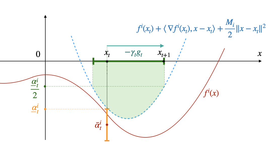
Figure 1: Illustration of the adaptivity. Step size $\gamma_{t}$ is chosen such that the quadratic smoothness upper bound (black) on the constraint guarantees $f^{i}(x_{t+1})\leq f^{i}(x_{t})/2$. $\underline{\alpha}_{t}^{i}$ is the lower bound on $\alpha_{t}^{i}=-f^{i}(x_{t})$, constructed based on the mean estimator $\bar{\alpha}_{t}^{i}$. By the orange interval we denote the confidence interval for $\alpha_{t}^{i}$. By the green interval we denote the adaptive region for $x_{t+1}$ based on the requirement $f^{i}(x_{t+1})\leq f^{i}(x_{t})/2$.

Then, finally, we set the step-size to:

$$\gamma_{t}=\min\left\{\min_{i\in[m]}\left\{\frac{\underline{\alpha}^{i}_{t}}{2|\hat{\theta}^{i}_{t}|+\sqrt{\underline{\alpha}_{t}^{i}M_{i}}}\right\}\frac{1}{\|g_{t}\|},\frac{1}{\hat{M}_{2}(x_{t})}\right\}.$$ (14)

3.3.3 Basic algorithm

To sum up, below we propose our basic algorithm, but emphasize that it can be instantiated differently for different problem classes. We showcase possible instantiations of LB-SGD  in following Section 4.
Algorithm 2 LB-SGD($x_{0},{\color[rgb]{0,0,0}\eta},T{\color[rgb]{0,0,0},n}$) 1:  Input: $M_{i},\sigma_{i},\hat{\sigma}_{i},\hat{b}_{i}\in\mathbb{R}_{+}\leavevmode\nobreak\ \forall i\in\{0,\ldots,m\},$ $R\in\mathbb{R}_{+}$, $\eta\in\mathbb{R}_{+}$, $n\in\mathbb{N}$, $T\in\mathbb{N}$, $\delta\in[0,1]$; 2:  for $t=1,\ldots,T$  do 3:     Set $g_{t}$ $\leftarrow\mathcal{O}_{\eta}(x_{t},n)$ by taking a batch of measurements of size $n$ at $x_{t}$; 4:     Compute lower bounds $\underline{\alpha}_{t}^{i}:=\bar{\alpha}_{t}^{i}-\sigma_{i}(n)\sqrt{\ln\frac{1}{\delta}}$ $,\leavevmode\nobreak\ \forall i\in[m]$; 5:     Compute upper bounds $\hat{\theta}_{t}^{i}=|\langle G^{i}_{n}(x,\xi),\frac{g_{t}}{\|g_{t}\|}\rangle|+\hat{b}_{i}+\hat{\sigma}_{i}(n)\sqrt{\log\frac{1}{\delta}},\leavevmode\nobreak\ \forall i\in[m]$; 6:     Compute $\hat{M}_{2}(x_{t})$ using (12); 7:     $\gamma_{t}\leftarrow\min\left\{\min_{i\in[m]}\left\{\frac{\underline{\alpha}^{i}_{t}}{2|\hat{\theta}^{i}_{t}|+\sqrt{\underline{\alpha}_{t}^{i}M_{i}}}\right\}\frac{1}{\|g_{t}\|},\frac{1}{\hat{M}_{2}(x_{t})}\right\}$; 8:     $x_{t+1}\leftarrow x_{t}-\gamma_{t}g_{t}$; 9:  end for 10:  Output: $\{x_{1},\ldots,x_{T}\}$. In the above, the input parameters are: the smoothness constant $M_{i}$ of each function $f^{i}$ for $i\in\{0,\ldots,m\}$, the bound on the variance of its value measurements $\sigma^{2}_{i}$, the bound on the variance of its gradient measurements $\hat{\sigma}^{2}_{i}$ and the upper bound on the bias of its gradient measurements $\hat{b}_{i}$, the bound on the diameter $R$ of the set $\mathcal{X}$, the log barrier parameter $\eta$, the number of measurements per iteration $n$, the number of iterations $T$, and the confidence parameter $\delta$.

3.4 Safety

From the safety side, the adaptive step-size $\gamma_{t}$ automatically guarantees the safety of all the iterates due to construction, for any procedure generating the iterations in the form $x_{t+1}=x_{t}-\gamma_{t}g_{t}$ where $\gamma_{t}$ is bounded by (14). The feasibility of the optimization trajectory we guarantee with probability at least $1-\hat{\delta}$ with $\hat{\delta}:=mT\delta.$

Theorem 4

Let $T>0$ denote the total number of iterations of the form (7), and $\hat{\delta}\in(0,1)$ denote the target confidence level. Then, for LB-SGD  with parameter $\delta\leq\hat{\delta}/mT$, all the query points $x_{t}$ are feasible with probability greater than $1-\delta$.

Proof  Due to the adaptive step size $\gamma_{t}$, we have $x_{t}\in\mathcal{X}$ implies $x_{t+1}\in\mathcal{X}$ (see Lemma 3) since $f^{i}(x_{t+1})\leq\frac{f^{i}(x_{t})}{2}$ with probability $1-\delta$. Then, using $x_{0}\in\mathcal{X}$ and Boole’s inequality, we conclude that the whole optimization trajectory $\{x_{t}\}_{t\in[T]}$ is feasible with probability at least $1-mT\delta\geq 1-\hat{\delta}$.  

4 Method Variants and Convergence Analysis

First of all, let us show the following general property of the log barrier method, important for the further convergence analysis of any problem type that we discuss.

4.1 Keeping a distance away from the boundary

Imagine that $\underline{\alpha}_{t}^{i}$ becomes $0$ for some iteration $t$ during the learning. That would lead to $\gamma_{t}=0$, and the algorithm will stop without converging, since there is no safe non-zero step-size. Moreover, the log barrier gradient at that point simply blows up. However, we can lower bound the step sizes $\gamma_{t}$ if we can provide a lower bound on $\underline{\alpha}_{t}^{i}$ for all $t>0$ during the learning with high probability:

Lemma 5

If $\underline{\alpha}_{t}^{i}\geq c\eta$ for $c>0$, then we have $\mathbb{P}\{\gamma_{t}\geq C\eta\}\geq 1-\delta$ with $C$ defined by

$$C:=\frac{c}{2L^{2}(1+\frac{m}{c})}\frac{1}{\max\left\{{\color[rgb]{0,0,0}4}+\frac{{\color[rgb]{0,0,0}5}Mc\eta}{L^{2}},1+\sqrt{\frac{Mc\eta}{4L^{2}}}\right\}}.$$ (15)

The proof is shown in Appendix A.6.

Therefore, for convergence, we need to show that our algorithm’s iterates $x_{t}$ do not only stay inside the feasible set, but moreover keep a distance away from the boundary. Keeping distance is the key property, guaranteeing the regularity of the log barrier function in the sense of a bounded gradient norm, bounded local smoothness and bounded variance. For the exact information case without noise, the adaptive gradient descent on the log barrier is shown to converge without stating this property explicitly (Hinder and Ye, 2018). However, in the stochastic case, this property becomes crucial for establishing stable convergence. It guarantees that the method pushes the iterates $x_{t}$ away from the boundary of the set $\mathcal{X}$ as soon as they come too close to the boundary. We formulate it below.

Lemma 6

Let Assumptions 2 and 3 hold, Assumption 4 hold with $\rho\geq\eta$, and let $\hat{\sigma}_{i}(n)\leq\frac{\alpha_{t}^{i}L}{\eta\sqrt{\ln\frac{1}{\delta}}}$, $\hat{b}_{i}\leq\frac{\alpha_{t}^{i}L}{2\eta}$, and $\sigma_{i}(n)\leq\frac{(\alpha_{t}^{i})^{2}}{2\eta\sqrt{\ln\frac{1}{\delta}}}$. Then, we can show that for all $x_{t}$ for all iterations $t\in[T]$ generated by the optimization process $x_{t+1}=x_{t}-\gamma_{t}g_{t}$ the following holds: $\mathbb{P}\{\forall t\in[T]\leavevmode\nobreak\ \min_{i\in[m]}\underline{\alpha}_{t}^{i}\geq c\eta\}\geq 1-\hat{\delta}$ with

$$c:={\color[rgb]{0,0,0}\frac{1}{2}}\left(\frac{l}{4L(2m+1)}\right)^{m},$$

where $l>0$ is defined as in Assumption 4.

Proof  First, let us note the following fact demonstrating that the product of the smallest absolute constraint values is not decreasing if $x_{t}$ is close enough to the boundary.

Fact 1

Let Assumptions 2, 3 hold, Assumption 4 hold with $\rho\geq\eta$, and let $\hat{\sigma}_{i}(n)\leq\frac{\alpha_{t}^{i}L}{2\eta\sqrt{\ln\frac{1}{\delta}}}$, $\hat{b}_{i}\leq\frac{\alpha_{t}^{i}L}{2\eta}$, and $\sigma_{i}(n)\leq\frac{(\alpha_{t}^{i})^{2}}{2\eta\sqrt{\ln\frac{1}{\delta}}}$. If at iteration $t$ we have $\min_{i\in[m]}\alpha_{t}^{i}\leq\bar{c}\eta$ with $\bar{c}:=\frac{l}{L}\frac{1}{2m+1}$, then, for the next iteration $t+1$ we get $\prod_{i\in\mathcal{\mathcal{I}}}\alpha_{t+1}^{i}\geq\prod_{i\in\mathcal{\mathcal{I}}}\alpha_{t}^{i}$ for any $\mathcal{I}:\mathcal{I}_{t}\subseteq\mathcal{I}$ with $\mathcal{I}_{t}:=\{i\in[m]:\alpha_{t}^{i}\leq\eta\}$ with probability $1-\delta$.

For the proof see Appendix A.5.

Note that if $\min_{i\in[m]}\alpha_{t}^{i}\geq\bar{c}\eta$ for all $t\geq 0$, then the statement of the Lemma holds automatically. Now, consider a consecutive set of steps $t=\{t_{0},\ldots,t_{k}\}$ on whose $\min_{i\in[m]}\alpha_{t}^{i}\leq\bar{c}\eta$. By definition, and using Fact 1, for any $t\in\{t_{0},\ldots,t_{k}\}$ we have with probability $1-\delta$

$$\prod_{i\in\mathcal{I}_{t+1}}\alpha_{t+1}^{i}=\frac{\prod_{i\in\mathcal{I}_{t}\cup\mathcal{I}_{t+1}}\alpha_{t+1}^{i}}{\prod_{i\in\mathcal{I}_{t}\setminus\mathcal{I}_{t+1}}\alpha_{t+1}^{i}}\geq\frac{\prod_{i\in\mathcal{I}_{t}\cup\mathcal{I}_{t+1}}\alpha_{t}^{i}}{\prod_{i\in\mathcal{I}_{t}\setminus\mathcal{I}_{t+1}}\alpha_{t+1}^{i}}.$$

By induction, applying the above sequentially for all $t\in\{t_{0},\ldots,t_{k}\}$ we can get

$$\prod_{i\in\mathcal{I}_{t_{k}}}\alpha_{t_{k}}^{i}\geq\frac{\prod_{i\in\mathcal{I}_{t_{k}}\cup\mathcal{I}_{t_{k-1}}\cup\ldots\cup\mathcal{I}_{t_{0}}}\alpha_{t_{0}}^{i}}{\prod_{i\in\mathcal{I}_{t_{k-1}}\setminus\mathcal{I}_{t_{k}}}\alpha_{t_{k}}^{i}\prod_{i\in\mathcal{I}_{t_{k-2}}\setminus(\mathcal{I}_{t_{k}}\cup\mathcal{I}_{t_{k-1}})}\alpha_{t_{k-1}}^{i}\ldots\prod_{i\in\mathcal{I}_{t_{0}}\setminus(\mathcal{I}_{t_{k}}\cup\ldots\cup\mathcal{I}_{t_{1}})}\alpha_{t_{1}}^{i}}$$

with probability $1-\hat{\delta}$ (using Boole’s inequality).

Note that by definition of $\mathcal{I}_{t}$: $\alpha_{t}^{i}\leq\eta$ for $i\in\mathcal{I}_{t}$. At the same time, due to the step size choice, we have $\alpha_{t+1}^{i}\leq 2\alpha_{t}^{i}\leq 2\eta.$ Also, note that the sum of the set cardinalities in the denominator equals to the cardinality of the set $|\mathcal{I}_{t_{0}}\cup\ldots\cup\mathcal{I}_{t_{k}}\setminus\mathcal{I}_{t_{k}}|$. Hence, with probability $1-\hat{\delta}$

$$\prod_{i\in\mathcal{I}_{t_{k}}}\alpha_{t_{k}}^{i}\geq\frac{\prod_{i\in\mathcal{I}_{t_{k}}\cup\mathcal{I}_{t_{k-1}}\cup\ldots\cup\mathcal{I}_{t_{0}}}\alpha_{t_{0}}^{i}}{(2\eta)^{|\mathcal{I}_{t_{0}}\cup\ldots\cup\mathcal{I}_{t_{k}}\setminus\mathcal{I}_{t_{k}}|}}.$$

Thus, for any $j\in\mathcal{I}_{t_{k}}$ we get the bound:

$$\alpha_{t_{k}}^{j}\geq\frac{\prod_{i\in\mathcal{I}_{t_{k}}\cup\mathcal{I}_{t_{k-1}}\cup\ldots\cup\mathcal{I}_{t_{0}}}\alpha_{t_{0}}^{i}}{(2\hat{c}\eta)^{|\mathcal{I}_{t_{0}}\cup\ldots\cup\mathcal{I}_{t_{k}}\setminus j|}}\geq\frac{(\bar{c}\eta/2)^{|\mathcal{I}_{t_{0}}\cup\ldots\cup\mathcal{I}_{t_{k}}|}}{2^{|\mathcal{I}_{0}\cup\ldots\cup\mathcal{I}_{t_{k}}|-1}}\geq\left(\frac{\bar{c}}{4}\right)^{m}\eta.$$

Since $\sigma_{i}(n)\leq\frac{\alpha_{t}^{i}}{2\sqrt{\ln\frac{1}{\delta}}}$, we get that $\underline{\alpha}_{t}^{i}\geq\frac{\alpha_{t}^{i}}{2}\geq\frac{1}{2}\left(\frac{\bar{c}}{4}\right)^{m}\eta$ with probability $1-\delta$. Using the definition $\bar{c}:=\frac{l}{L}\frac{1}{2m+1},$ we obtain the statement of the lemma.  

4.2 Stochastic non-convex problems

For the non-convex problem we analyse LB-SGD$(x_{0}{\color[rgb]{0,0,0},\eta},T{\color[rgb]{0,0,0},n})$ with the fixed parameter $\eta$, that uses the stopping criterion

$$\|g_{t}\|\leq 3\eta/4$$ (16)

and outputs $x_{\hat{t}}$ with $\hat{t}$ corresponding to $\arg\min_{t\in T}\|g_{t}\|$.

4.2.1 Stationarity criterion in the non-convex case

Similarly to Usmanova et al. (2020), we can state that in general case small gradient of the log barrier with parameter $\eta$ leads to an $\eta$-approximate KKT point of the constrained problem. Let us set the pair of primal and dual variables to $(x,\lambda):=\left(x,\left[\frac{\eta}{-f^{1}(x)},\ldots,\frac{\eta}{-f^{m}(x)}\right]^{T}\right)$. Then, it satisfies:

$$1)\leavevmode\nobreak\ \|\nabla_{x}\mathcal{L}(x,\lambda)\|=\|\nabla B_{\eta}(x)\|;$$

$$2)\leavevmode\nobreak\ \lambda^{i}(-f^{i}(x))=\frac{\eta}{-f^{i}(x)}(-f^{i}(x))=\eta;$$

$$3)\leavevmode\nobreak\ \lambda^{i}\geq 0,-f^{i}(x)\geq 0,\leavevmode\nobreak\ i\in[m].$$

This insight immediately implies the following Lemma.

Lemma 7

Consider problem (P) under Assumptions 2, and 3. Let $\hat{x}$ be an $\eta$-approximate solution to $\min_{x\in\mathbb{R}^{d}}B_{\eta}(x)$, the $\eta$-log barrier approximation of (P), such that $\|\nabla B_{\eta}(\hat{x})\|\leq\eta$. Then, $\hat{x}$ is an $\eta$-approximate KKT point to the original problem (P).

Thus, we can use a small log barrier norm to guarantee stationarity for problem (P).

4.2.2 Convergence for the non-convex problem

Then, we get the following convergence result:

Theorem 8

After at most $T$ iterations of LB-SGD with $T\leq{\color[rgb]{0,0,0}11}\frac{B_{\eta}(x_{0})-\min_{x}B_{\eta}(x)}{C\eta^{3}},$ and with $\sigma_{i}(n)=O({\color[rgb]{0,0,0}\eta^{2}})$, $\hat{\sigma}_{i}(n)=O({\color[rgb]{0,0,0}\eta}),$ and $\hat{b}_{i}=O({\color[rgb]{0,0,0}\eta}),$ for the output $x_{\hat{t}}$ with $\hat{t}=\arg\min_{t\in T}\|g_{t}\|$ we have

$$\mathbb{P}\left\{\|\nabla B_{\eta}(x_{\hat{t}})\|\leq\eta\right\}\geq 1-\hat{\delta}$$ (17)

Therefore, given $\sigma_{i}(n)=\frac{\sigma_{i}}{\sqrt{n}}$ (3) and $\hat{\sigma}_{i}(n)=\frac{\hat{\sigma}_{i}}{\sqrt{n}}$ ( 4), for constant $\hat{\sigma}_{i},\sigma_{i}$, we require $n=O(\frac{1}{\eta^{4}})$ oracle calls per iteration, and $N=O(\frac{1}{\eta^{7}})$ calls of the first-order stochastic oracle in total. Using Lemma 7, we get that $x_{\hat{t}}$ is an $\varepsilon$-approximate KKT point to the original problem (P) with $\varepsilon=\eta$.

Remark

Lower bound in the unconstrained non-safe case. In a well-known model where algorithms access smooth, non-convex functions through queries to an unbiased stochastic gradient oracle with bounded variance, Arjevani et al. (2019) prove that in the worst case any algorithm requires at least $\varepsilon^{-4}$ queries to find an $\varepsilon$ stationary point. Although, they allow $d$ to depend on $\varepsilon$. Therefore, we "pay" extra $\varepsilon^{-3}$ measurements for safety. From the methodology point of view, this happens due to the non-smoothness of the log-barrier on the boundary and the fact that the noise of the barrier gradient estimator is very sensitive to how close the iterates $x_{t}$ are to the boundary.

Proof 
Step 1. Bounding number of iterations $T$. First, let us denote $\hat{\gamma}_{t}:=\gamma_{t}\|g_{t}\|.$ At each iteration of Algorithm 2 with the fixed $\eta$ the value of the logarithmic barrier decreases at least by the following value:

$$B_{\eta}(x_{t})-B_{\eta}(x_{t+1}) \overset{\scriptsize1⃝}{\geq}\gamma_{t}\left\langle\nabla B_{\eta}(x_{t}),g_{t}\right\rangle-\frac{1}{2}M_{2}(x_{t})\gamma_{t}^{2}\|g_{t}\|^{2}$$

$$=\hat{\gamma}_{t}\langle\Delta_{t},\frac{g_{t}}{\|g_{t}\|}\rangle+\hat{\gamma}_{t}\left(1-\frac{M_{2}(x_{t})\gamma_{t}}{2}\right)\|g_{t}\|$$

$$\overset{\scriptsize2⃝}{\geq}\frac{1}{2}\hat{\gamma}_{t}\|g_{t}\|-\hat{\gamma}_{t}\|\Delta_{t}\|.$$ (18)

In the above, $M_{2}(x)$ is the local smoothness constant that we bound by (12). The first inequality $\scriptsize1⃝$ is due to the local smoothness of the barrier. $\scriptsize2⃝$ is due to the fact that $\mathbb{P}\{\gamma_{t}\leq\frac{1}{M_{2}(x_{t})}\}\geq 1-\delta,$ given $x_{t}\in Int(\mathcal{X})$. Summing up the above inequalities (4.2.2) for $t\in[T]$, we obtain the second inequality below:

$${\color[rgb]{0,0,0}T\min_{t\in[T]}\hat{\gamma}_{t}\left(\frac{1}{2}\|g_{t}\|-\|\Delta_{t}\|\right)}\leq\sum_{t\in[T]}\hat{\gamma}_{t}\left(\frac{1}{2}\|g_{t}\|-\|\Delta_{t}\|\right) \leq B_{\eta}(x_{0})-\min_{x\in\mathcal{\mathcal{missing}}X}B_{\eta}(x).$$

In the above, the first inequality is due to the fact that the minimum of summands is smaller than any of the summands. Recall that we stop the algorithm as soon as $\|g_{t}\|\leq 3\eta/4$, as stated in the beginning of the section in (16). Hence, for all $T$ iterations $t\in[T]$ with $\|g_{t}\|\geq 3\eta/4$ we have $\hat{\gamma}_{t}\geq 0.75\eta\gamma_{t}$. Therefore, we get:

$${\color[rgb]{0,0,0}T}{\color[rgb]{0,0,0}\leq\frac{B^{\eta}(x_{0})-\min_{x}B^{\eta}(x)}{{\color[rgb]{0,0,0}\min_{t\in[T]}}\{\hat{\gamma}_{t}\left(0.5\|g_{t}\|-\|\Delta_{t}\|\right)\}}}\leq\frac{B^{\eta}(x_{0})-\min_{x}B^{\eta}(x)}{0.75\eta{\color[rgb]{0,0,0}\min_{t\in[T]}}\{\gamma_{t}\left(0.5\|g_{t}\|-\|\Delta_{t}\|\right)\}}.$$ (19)

We have to obtain the lower bound on the denominator. Using the result of Lemmas 5 and 6, for all $t\in{\color[rgb]{0,0,0}[T]}$ we have $\gamma_{t}\geq C\eta$.
Step 2. Bounding $\|\Delta_{t}\|$. Next, we have to upper bound $\|\Delta_{t}\|$ with high probability. Recall from Lemma 1 (9):

$$\mathbb{P}\left\{\|\Delta_{t}\|\leq b_{0}+\hat{\sigma}_{0}(n)\sqrt{\ln\frac{1}{\delta}}+\sum_{i=1}^{m}\frac{\eta}{\bar{\alpha}_{t}^{i}}\left(\hat{b}_{i}+\hat{\sigma}_{i}(n)\sqrt{\ln\frac{1}{\delta}}\right)+\sum_{i=1}^{m}L_{i}\frac{\eta\sigma_{i}(n)}{\alpha_{t}^{i}\bar{\alpha}_{t}^{i}}\sqrt{\ln\frac{1}{\delta}}\right\}\geq 1-\delta.$$

Hence, we can guarantee $\mathbb{P}\{\|\Delta_{t}\|\leq\frac{\eta}{4}\forall t\}\geq 1-\hat{\delta}$ if for all $i\in[m]$

$$\hat{\sigma}_{0}(n) \leq\frac{\eta}{4{\color[rgb]{0,0,0}(3m+2)}\sqrt{\ln\frac{1}{\delta}}},\hat{\sigma}_{i}(n)\leq\frac{\underline{\alpha}_{t}^{i}}{4{\color[rgb]{0,0,0}(3m+2)}\sqrt{\ln\frac{1}{\delta}}},$$ (20)

$$\hat{b}_{0} \leq\frac{\eta}{4{\color[rgb]{0,0,0}(3m+2)}},\hat{b}_{i}\leq\frac{\underline{\alpha}_{t}^{i}}{4{\color[rgb]{0,0,0}(3m+2)}},\sigma_{i}(n)\leq\frac{(\underline{\alpha}_{t}^{i})^{2}}{4{\color[rgb]{0,0,0}(3m+2)}L\sqrt{\ln\frac{1}{\delta}}},$$ (21)

(using the Boolean inequality). Using the lower bound on $\underline{\alpha}_{t}^{i}$ by Lemma 6, we get that for all $i\in[m]$ we require $\hat{\sigma}_{i}(n)=O(\eta)$, $\sigma_{i}(n)=O(\eta^{2})$, $\hat{b}_{i}=O(\eta).$
Step 3. Finalising the bounds. Then, using $\|g_{t}\|\leq 3\eta/4$ for all $t\in[T]$, we can claim that with high probability for any $t\in[T]$ the following holds

$$0.5\|g_{t}\|-\|\Delta_{t}\|\geq\frac{3}{8}\eta-\frac{1}{4}\eta=\frac{\eta}{8}.$$

Combining it with inequality (19), the algorithm stops after at most $T$ iterations with

$$T\leq 8\frac{B_{\eta}(x_{0})-\min_{x}B_{\eta}(x)}{{\color[rgb]{0,0,0}0.75}C\eta^{3}}{\color[rgb]{0,0,0}\leq 11\frac{B_{\eta}(x_{0})-\min_{x}B_{\eta}(x)}{C\eta^{3}}}.$$

Finally, using $\mathbb{P}\{\|\Delta_{t}\|\leq\frac{\eta}{4}\forall t\}\geq 1-\hat{\delta}$ and the stopping criterion $\|g_{t}\|\leq 3\eta/4$ (16), we obtain

$$\mathbb{P}\left\{\|\nabla B_{\eta}(x_{\hat{t}})\|{\color[rgb]{0,0,0}\leq\|g_{\hat{t}}\|+\|\Delta_{\hat{t}}\|}\leq\eta\right\}\geq 1-\hat{\delta}.$$

 

4.3 Stochastic convex problems

For the convex case, we propose to use LB-SGD($x_{0},{\color[rgb]{0,0,0}\eta},T{\color[rgb]{0,0,0},n}$) with the output: $\bar{x}_{T}:=\frac{\sum_{t=1}^{T}\gamma_{t}x_{t}}{\sum_{t=1}^{T}\gamma_{t}}$. Next, we discuss the optimality criterion for convex problems.

4.3.1 Optimality criterion in the convex case

In the convex case, we can relate an approximate solution of the log barrier problem to an $\varepsilon$-approximate solution of the original problem in terms of the objective value.

Assumption 5

The objective and the constraint functions $f^{i}(x)$ for all $i\in\{0,\ldots,m\}$ are convex.

Note that Assumption 3 implies non-emptiness on $Int(\mathcal{X})$ which is called Slater Constraint Qualification. In the convex setting, it in turn implies the extended MFCQ:

Fact 2

Let Assumptions 1, 3, and 5 hold. Then, Assumption 4 holds with $s_{x}:=\frac{x-x_{0}}{\|x-x_{0}\|}$, such that $\langle\nabla f^{i}(x),s_{x}\rangle\geq\frac{\beta-\rho}{R}$ for all $i\in\mathcal{I}_{\rho}(x)$ for any $0<\rho<\beta$ .

Proof  Indeed, for any point $x\in\mathcal{X}$ and for any convex constraint $f^{i}$ such that $f^{i}(x)\geq-\rho$, due to convexity we have $f^{i}(x)-f^{i}(x_{0})\leq\langle\nabla f^{i}(x),x-x_{0}\rangle.$ Given the bounded diameter of the set $\|x_{0}-x\|\leq R$, we get $\langle\nabla f^{i}(x),s_{x}\rangle\geq\frac{\beta-\rho}{R}$.  
Then, we can relate an $\eta$-approximate solution by the log barrier value with an $\varepsilon$-approximate solution for the original problem, where $\varepsilon$ depends on $\eta$ linearly up to a logarithmic factor. We formulate that in the following lemma:

Lemma 9

Consider problem (P) under Assumptions 1, 2, 3, and the convexity Assumption 5. Assume that $\hat{x}$ is an $\eta$-approximate solution to the $\eta$-log barrier approximation, that is,

$$B_{\eta}(\hat{x})-B_{\eta}(x^{*}_{\eta})\leq\eta,$$

where $x^{*}_{\eta}$ is a solution of the $\min B_{\eta}$ minimization problem, with $\eta\leq\beta/2$. Then, $\hat{x}$ is an $\varepsilon$-approximate solution to the original problem (P) with $\varepsilon=\eta(m+1)+\eta m\log\left(\frac{2mLR\hat{\beta}}{\eta\beta}\right)$, that is, $f^{0}(\hat{x})-\min_{x\in\mathcal{X}}f^{0}(x)\leq\varepsilon,$ where $\hat{\beta}>0$ is such that $\forall i\in[m]\forall x\in\mathcal{X}\leavevmode\nobreak\ |f^{i}(x)|\leq\hat{\beta}.$ Since the constraints are smooth and the set $\mathcal{X}$ is bounded, such $\hat{\beta}$ exists.

Proof sketch

Let $\hat{x}$ be an approximately optimal point for the log barrier: $B_{\eta}(\hat{x})-B_{\eta}(x^{*}_{\eta})\leq\eta,$ and $x^{*}_{\eta}$ be an optimal point for the log barrier. Then, using the definition, we can bound: $f^{0}(\hat{x})-f^{0}(x^{*}_{\eta})\leq\eta+\eta\sum_{i=1}^{m}-\log\frac{-f^{i}(x^{*}_{\eta})}{-f^{i}(\hat{x})}.$ Combining Fact 2 with the first order stationarity criterion, we can derive: $\min_{i\in[m]}\{-f^{i}(x^{*}_{\eta})\}\geq\frac{\eta\beta}{2mLR}.$ Hence, combining the above two inequalities, we get the following relation of point $\hat{x}$ and point $x^{*}_{\eta}$: $f^{0}(\hat{x})-f^{0}(x^{*}_{\eta})\leq\eta\left(1+m\log\left(\frac{2mLR\hat{\beta}}{\eta\beta}\right)\right)$ using $-f^{i}(\hat{x})\leq\hat{\beta}$. Using the Lagrangian definition for stationarity of the optimal point of the initial problem $x^{*}$, we get the following relation between $x^{*}$ and $x^{*}_{\eta}$: $f^{0}(x^{*}_{\eta})-f^{0}(x^{*})\leq m\eta.$ Combining it with the above, we get the statement of the Lemma

$$f^{0}(\hat{x})-\min_{x\in\mathcal{X}}f^{0}(x)\leq\eta+\eta m\log\left(\frac{2mLR\hat{\beta}}{\eta\beta}\right)+m\eta.$$

For the full proof see Appendix A.7.

4.3.2 Convergence in the convex case

As already discussed in the optimality criterion Section 4.3.1, for the convex problem we only require the convergence in terms of the value of the log barrier. Thus, we get the following convergence result for this method.

Theorem 10

Let Assumptions 1, 2, 3, 5 hold, $B_{\eta}(x):=f^{0}(x)-\eta\sum_{i=1}^{m}\log(-f^{i}(x))$ be a log barrier function with parameter $\eta>0$, and $x_{0}\in\mathbb{R}^{d}$ be the starting point. Let $x^{*}_{\eta}$ be a minimizer of $B_{\eta}(x)$. Then, after $T\geq\frac{\|x_{0}-x_{\eta}^{*}\|^{2}}{C\eta^{2}}$ iterations of LB-SGD, and with $\sigma_{i}(n)=O(\frac{\eta^{2}}{R})$, $\hat{\sigma}_{i}(n)=O(\frac{\eta}{R}),$ and $\hat{b}_{i}=O(\frac{\eta}{R}),$ for the point $\bar{x}_{T}:=\frac{\sum_{t=1}^{T}\gamma_{t}x_{t}}{\sum_{t=1}^{T}\gamma_{t}}$ we obtain:

$$\mathbb{P}\left\{B_{\eta}(\bar{x}_{T})-B_{\eta}(x^{*}_{\eta})\leq\eta\right\}\geq 1-\hat{\delta}.$$

For the noise with constant variances $\hat{\sigma}_{i},\sigma_{i}$, given $\sigma_{i}(n)=\frac{\sigma_{i}}{\sqrt{n}}$ (3) and $\hat{\sigma}_{i}(n)=\frac{\hat{\sigma}_{i}}{\sqrt{n}}$ ( 4), we require $n=O(\frac{1}{\eta^{4}})$ oracle calls per iteration, and $O(\frac{1}{\eta^{6}})$ measurements of the first-order oracle in total. Using Lemma 9 we get $\bar{x}_{T}$ is an $\varepsilon$-approximate solution to the original problem (P) with $\varepsilon=\eta(m+1)+\eta m\log\left(\frac{2mLR\hat{\beta}}{\eta\beta}\right)$, that is, $f^{0}(\hat{x})-\min_{x\in\mathcal{X}}f^{0}(x)\leq\varepsilon.$

Proof  Note the following

$$B_{\eta}(x_{t+1})-B_{\eta}(x^{*}_{\eta}) \overset{\scriptsize1⃝}{\leq}B_{\eta}(x_{t})+\langle\nabla B_{\eta}(x_{t}),x_{t+1}-x_{t}\rangle+\frac{M_{2}(x_{t})}{2}\|x_{t}-x_{t+1}\|^{2}-B_{\eta}(x^{*}_{\eta})$$

$$\overset{\scriptsize2⃝}{\leq}\langle\nabla B_{\eta}(x_{t}),x_{t+1}-x_{t}\rangle+\frac{M_{2}(x_{t})}{2}\|x_{t}-x_{t+1}\|^{2}+\langle\nabla B_{\eta}(x_{t}),x_{t}-x^{*}_{\eta}\rangle$$

$$=\frac{M_{2}(x_{t})}{2}\|x_{t}-x_{t+1}\|^{2}+\langle g_{t},x_{t+1}-x^{*}_{\eta}\rangle-\langle\Delta_{t},x_{t+1}-x^{*}_{\eta}\rangle$$

$$\overset{\scriptsize3⃝}{\leq}\frac{\|x_{t}-x^{*}_{\eta}\|^{2}}{2\gamma_{t}}-\frac{\|x_{t+1}-x^{*}_{\eta}\|^{2}}{2\gamma_{t}}-\left(\frac{1}{2\gamma_{t}}-\frac{M_{2}(x_{t})}{2}\right)\|x_{t+1}-x_{t}\|^{2}-\langle\Delta_{t},x_{t+1}-x^{*}_{\eta}\rangle$$

$$\overset{\scriptsize4⃝}{\leq}\frac{\|x_{t}-x^{*}_{\eta}\|^{2}}{2\gamma_{t}}-\frac{\|x_{t+1}-x^{*}_{\eta}\|^{2}}{2\gamma_{t}}-\langle\Delta_{t},x_{t+1}-x^{*}_{\eta}\rangle.$$

The first inequality $\scriptsize1⃝$ is due to the $M_{2}(x_{t})$-local smoothness of the log barrier, the second one $\scriptsize2⃝$ is due to convexity. The third inequality $\scriptsize3⃝$ uses the fact that: $\forall u\in\mathbb{R}^{d}:\leavevmode\nobreak\ \langle g_{t},x_{t+1}-u\rangle=\frac{\|x_{t}-u\|^{2}}{2\gamma_{t}}-\frac{\|x_{t+1}-u\|^{2}}{2\gamma_{t}}-\frac{\|x_{t+1}-x_{t}\|^{2}}{2\gamma_{t}}.$ And the last one $\scriptsize4⃝$ is due to $\gamma_{t}\leq\frac{1}{M_{2}(x_{t})}$. By multiplying both sides by $\gamma_{t}$, we get:

$$2\gamma_{t}(B_{\eta}(x_{t+1})-B_{\eta}(x^{*}_{\eta})) \leq\|x_{t}-x^{*}_{\eta}\|^{2}-\|x_{t+1}-x^{*}_{\eta}\|^{2}-2\gamma_{t}\langle\Delta_{t},x_{t+1}-x^{*}_{\eta}\rangle.$$ (22)

Then, by summing up the above for all $t\in[T]$ we get, and using the Jensen’s inequality:

$$B_{\eta}\left(\frac{\sum_{t=1}^{T}\gamma_{t}x_{t}}{\sum\gamma_{t}}\right)-B_{\eta}(x^{*}_{\eta}) \leq\frac{1}{\sum_{t=1}^{T}\gamma_{t}}\sum_{t=1}^{T}\gamma_{t}(B_{\eta}(x_{t})-B_{\eta}(x^{*}_{\eta}))$$

$$\leq\frac{1}{2\sum_{t=1}^{T}\gamma_{t}}\sum_{t=1}^{T}\left(\|x_{t}-x^{*}_{\eta}\|^{2}-\|x_{t+1}-x^{*}_{\eta}\|^{2}-2\gamma_{t}\langle\Delta_{t},x_{t+1}-x^{*}_{\eta}\rangle\right)$$

$$\leq\frac{\|x_{0}-x^{*}_{\eta}\|^{2}}{2\sum_{t=1}^{T}\gamma_{t}}-\frac{\sum_{t=1}^{T}\gamma_{t}\langle\Delta_{t},x_{t+1}-x^{*}_{\eta}\rangle}{2\sum_{t=1}^{T}\gamma_{t}}.$$ (23)

That is, we can bound the accuracy by

$$B_{\eta}\left(\bar{x}_{T}\right)-B_{\eta}(x^{*}_{\eta}) \leq\frac{\|x_{0}-x^{*}_{\eta}\|^{2}}{2\sum_{t=1}^{T}\gamma_{t}}+\frac{\max_{t}\langle\Delta_{t},x_{t+1}-x^{*}_{\eta}\rangle}{2}.$$ (24)

Using Lemma 5 we can prove for $\hat{\sigma}_{i}(n)\leq\frac{L\alpha_{t}^{i}}{3\eta\sqrt{\ln\frac{1}{\delta}}}$ that $\gamma_{t}\geq C\eta.$ Recall from Lemma 1 (9):

$$\mathbb{P}\left\{\|\Delta_{t}\|\leq b_{0}+\hat{\sigma}_{0}(n)\sqrt{\ln\frac{1}{\delta}}+\sum_{i=1}^{m}\frac{\eta}{\bar{\alpha}_{t}^{i}}\left(\hat{b}_{i}+\hat{\sigma}_{i}(n)\sqrt{\ln\frac{1}{\delta}}\right)+\sum_{i=1}^{m}L_{i}\frac{\eta\sigma_{i}(n)}{\alpha_{t}^{i}\bar{\alpha}_{t}^{i}}\sqrt{\ln\frac{1}{\delta}}\right\}\geq 1-\delta.$$

Hence, we can guarantee $\|\Delta_{t}\|\leq\frac{\eta}{R}$ for all $t\in[T]$ with probability $1-\hat{\delta}$ if for all $i\in[m]$

$$\hat{\sigma}_{0}(n) \leq\frac{\eta}{(3m+2)R\sqrt{\ln\frac{1}{\delta}}},\hat{\sigma}_{i}(n)\leq\frac{\underline{\alpha}_{t}^{i}}{(3m+2)R\sqrt{\ln\frac{1}{\delta}}},$$ (25)

$$\hat{b}_{0} \leq\frac{\eta}{(3m+2)R},\hat{b}_{i}\leq\frac{\underline{\alpha}_{t}^{i}}{(3m+2)R},\sigma_{i}(n)\leq\frac{(\underline{\alpha}_{t}^{i})^{2}}{(3m+2)LR\sqrt{\ln\frac{1}{\delta}}}.$$

Using the lower bound on $\underline{\alpha}_{t}^{i}$ by Lemma 6, we get that for all $i\in[m]$ we require $\hat{\sigma}_{i}(n)=O(\eta)$, $\sigma_{i}(n)=O(\eta^{2})$, $\hat{b}_{i}=O(\eta).$
Therefore, we get for the $\bar{x}_{T}$ the following bound on the accuracy:

$$B_{\eta}\left(\bar{x}_{T}\right)-B_{\eta}(x^{*}_{\eta}) \leq\frac{\|x_{0}-x^{*}_{\eta}\|^{2}}{TC\eta}+\frac{\max_{t}\|\Delta_{t}\|R}{2}\leq\frac{\|x_{0}-x^{*}_{\eta}\|^{2}}{TC\eta}+\frac{\eta}{2}.$$ (26)

Thus, for $T\geq\frac{\|x_{0}-x^{*}_{\eta}\|^{2}}{2C\eta^{2}}$ we obtain $\mathbb{P}\{B_{\eta}\left(\bar{x}_{T}\right)-B_{\eta}(x^{*}_{\eta})\leq\eta\}\geq 1-\hat{\delta}$. In order to satisfy conditions on the variance (25), we require at each iteration $n=O\left(\frac{1}{\eta^{4}}\right)$ measurements, and therefore $N=Tn=O(\frac{1}{\eta^{6}})$ measurements in total.  

4.4 Strongly-convex problems

For the strongly convex case, we make use of restarts with iteratively decreasing parameter $\eta_{k}$:
Algorithm 3 LB-SGD  with decreasing $\eta_{k}$ ($\eta\in\mathbb{R}_{+},\eta_{0}\in\mathbb{R}_{+},x_{0}\in\mathbb{R}^{d},\omega\in(0,1),\{T_{k}\},\{n_{k}\}$) 1:  Input: $M_{i}>0,i\in\{0,\ldots,m\},\eta_{0}\in\mathbb{R}_{+}$, $\hat{x}_{0}\leftarrow x_{0}$, ${\color[rgb]{0,0,0}K\leftarrow[\log_{\omega^{-1}}\frac{\eta_{0}}{\eta}]}$; 2:  for $k=1,\ldots,K$  do 3:     $\hat{x}_{k}\leftarrow$ LB-SGD$(\hat{x}_{k-1},{\color[rgb]{0,0,0}\eta_{k-1}},T_{k-1}{\color[rgb]{0,0,0},n_{k-1}})$; 4:     $\eta_{k}\leftarrow\omega\eta_{k-1},$ with $\omega\in(0,1)$; 5:  end for 6:  Output: $\hat{x}_{K}$.

In the above, $\eta_{0}$ is the initial log barrier parameter, $\omega\in(0,1)$ is the parameter reduction rate, $K$ is the number of rounds, $\eta=\eta_{K}$ is a barrier parameter at the last round, at every round $k$ we run LB-SGD with $T_{k}$ iterations and $n_{k}$ oracle calls per iteration.

4.4.1 Convergence

Theorem 11

Let Assumptions 1, 2, 3, 5 hold, and the log barrier function with parameter $\eta$: $B_{\eta}(x):=f^{0}(x)-\eta\sum_{i=1}^{m}\log(-f^{i}(x))$ be $\mu$-strongly-convex. Then, after at most $T=\frac{\|x_{0}-x^{*}_{\eta}\|^{2}}{C\eta_{0}^{2}}+\sum_{k=1}^{K}O(\frac{1}{C\mu\eta_{k}})=O\left(\frac{\log_{{\color[rgb]{0,0,0}\omega^{-1}}}\frac{\eta_{0}}{\eta}}{\mu\eta}\right)$ iterations of LB-SGD  with decreasing $\eta_{k}$ (Algorithm 3), and with $\sigma_{i}(n_{k})=O({\color[rgb]{0,0,0}\eta_{k}^{2}})$, $\hat{b}_{i}=O({\color[rgb]{0,0,0}\eta}),$ $\hat{\sigma}_{i}(n_{k})=O({\color[rgb]{0,0,0}\eta_{k}}),$ we obtain:

$$\mathbb{P}\left\{B_{\eta}(\hat{x}_{K})-\min_{x\in\mathcal{X}}B_{\eta}(x)\leq\eta\right\}\geq 1-\hat{\delta}$$

Hence, we require $n_{k}=O(\frac{1}{\eta_{k}^{4}})$ measurements per iteration at round $k$, and $N=\tilde{O}(\frac{1}{\eta^{5}})$ measurements of the first-order oracle in total. Using Lemma 9, we obtain that $\hat{x}_{K}$ is an $\varepsilon$-approximate solution to the original problem (P) with $\varepsilon=\eta(m+1)+\eta m\log\left(\frac{2mLR\hat{\beta}}{\eta\beta}\right).$

Proof 
Step 1. Important relations. Let $x^{*}_{\eta_{k}}$ be the unique minimizer of $B_{\eta_{k}}(x)$. We do the restarts with decreasing $\eta_{k}=\omega\eta_{k-1}$. From strong convexity, for any round $k>0$ we have:

$$\|\hat{x}_{k-1}-x^{*}_{\eta_{k}}\|^{2}\leq R_{k}^{2}:=\frac{B_{\eta_{k}}(\hat{x}_{k-1})-B_{\eta_{k}}(x^{*}_{\eta_{k}})}{\mu}.$$ (27)

Note that for all $x\in\mathcal{X}$ we have $B_{\eta_{k}}(x)\geq B_{\eta_{k-1}}(x)$ (without loss of generality assuming $-f^{i}(x)\leq\hat{\beta}\leq 1$). Consequently, $-B_{\eta_{k}}(x^{*}_{\eta_{k}})\leq-B_{\eta_{k-1}}(x^{*}_{\eta_{k-1}}).$ Therefore, using the definition of the log barrier, we can get:

$$B_{\eta_{k}}(\hat{x}_{k-1})-B_{\eta_{k}}(x^{*}_{\eta_{k}}) \leq B_{\eta_{k-1}}(\hat{x}_{k-1})-B_{\eta_{k-1}}(x^{*}_{\eta_{k-1}})+(\eta_{k-1}-\eta_{k})\sum_{i=1}^{m}-\log-f^{i}(\hat{x}_{k-1})$$

$$\leq B_{\eta_{k-1}}(\hat{x}_{{k-1}})-B_{\eta_{k-1}}(x^{*}_{\eta_{k-1}})+m\eta_{k-1}(1-\omega)\log\frac{1}{c\eta_{k}}.$$ (28)

Step 2. Induction over the rounds.
As an induction base, we can use Theorem 10 at the first round $k=1$, which claims that after $T_{0}\geq\frac{R^{2}}{C\eta_{0}}$ and $n_{0}=O\left(\frac{1}{\eta_{0}^{4}}\right)$ we get $B_{\eta_{0}}(\hat{x}_{0})-B_{\eta_{0}}(x^{*}_{\eta_{0}})\leq\eta_{0}.$
As an induction step, we assume that for some $k>0$, we have

$$B_{\eta_{k-1}}(\hat{x}_{k-1})-B_{\eta_{k-1}}(x^{*}_{\eta_{k-1}})\leq\eta_{k-1}.$$

This in turn, by section 4.4.1, leads to $B_{\eta_{k-1}}(\hat{x}_{k-1})-B_{\eta_{k-1}}(x^{*}_{\eta_{k}})\leq\eta_{k-1}(1+m(1-\omega)\log\frac{1}{c\eta_{k}}).$ Combining it with inequality (27), we get:

$$R_{k}^{2}\leq\frac{\eta_{k-1}(1+m(1-\omega)\log\frac{1}{c\eta_{k}})}{\mu}=\frac{\omega^{-1}\eta_{k}(1+(1-\omega)m\log\frac{1}{c\eta_{k}})}{\mu}.$$ (29)

Then, from Theorem 10, by the end of round $k$ we get the induction statement for the next step:

$$B_{\eta_{k}}(\hat{x}_{k})-B_{\eta_{k}}(x^{*}_{\eta_{k}})\leq\eta_{k},$$

for $\sigma_{i}(n_{k})\leq\frac{c^{2}\eta^{2}_{k}}{(3m+2)LR\sqrt{\ln\frac{1}{\delta}}}$, $\hat{b}^{i}\leq\frac{c\eta_{k}}{(3m+2)R}$, $\hat{\sigma}_{i}(n_{k})\leq\frac{c\eta_{k}}{(3m+2)R}\frac{1}{\sqrt{\ln 1/\delta}},$ and $T_{k}=[\frac{R_{k}^{2}}{C\eta_{k}^{2}}]$. Inserting the result of (29) into the bound on $T_{k}$, we require for $k>0$: $T_{k}=[\frac{\omega^{-1}+2m(\omega^{-1}-1)\log\frac{1}{c\eta_{k}}}{\mu C\eta_{k}}]$.
Thus, under the above conditions, the induction statement holds for all $k>0$, including $k=K$:

$$B_{\eta}(\hat{x}_{K})-B_{\eta}(x^{*}_{\eta})\leq\eta.$$

Step 3. Finalising the bounds. Recall that $\sigma^{i}(n_{k})=\frac{\sigma^{i}}{\sqrt{n_{k}}},\hat{\sigma}^{i}(n_{k})=\frac{\hat{\sigma}^{i}}{\sqrt{n_{k}}}.$ Then, we get that the required amount of measurements per iteration in order to get the required bounds on $\sigma^{i}(n_{k}),\hat{\sigma}^{i}(n_{k})$ is

$$n_{k}=\frac{4R^{2}(3m+2)^{2}}{\ln 1/\delta}\max\left\{\frac{(\hat{\sigma}^{i})^{2}}{c^{2}\eta_{k}^{2}},\frac{(\sigma^{i})^{2}L^{2}}{c^{4}\eta_{k}^{4}}\right\}=O\left(\frac{1}{\eta_{k}^{4}}\right).$$

We require the bias to be $\hat{b}^{i}\leq\frac{c\eta}{(3m+2)R}$ since $\eta\leq\eta_{k}$ for all $k\geq 0$.
Then, we need the following total number of iterations

$$T=T_{0}+\sum_{k=1}^{K}T_{k} =\frac{R^{2}}{C\eta_{0}^{2}}+\sum_{k=1}^{K}\frac{\omega^{-1}+m(\omega^{-1}-1)\log\frac{1}{c\eta_{k}}}{\mu C\eta_{k}}$$

$$\leq\frac{R^{2}}{C\eta_{0}^{2}}+\frac{\omega^{-1}+m(\omega^{-1}-1)\log\frac{1}{c\eta}}{\mu C\eta}\log{\color[rgb]{0,0,0}{}_{\omega^{-1}}}\frac{\eta_{0}}{\eta}=\tilde{O}\left(\frac{1}{\mu\eta}\right).$$

In total, we require $N$ measurements bounded as follows:

$${\color[rgb]{0,0,0}N} =T_{0}n_{0}+\sum_{k=1}^{K}T_{k}n_{k}\leq\frac{R^{2}}{C\eta_{0}^{6}}+\sum_{k=1}^{K}\frac{\omega^{-1}+m(\omega^{-1}-1)\log\frac{1}{c\eta_{k}}}{\mu C\eta_{k}}O\left(\frac{1}{\eta_{k}^{4}}\right)$$

$$\leq\frac{R^{2}}{C\eta_{0}^{6}}+\frac{\omega^{-1}+m(\omega^{-1}-1)\log\frac{1}{c\eta}}{\mu C\eta^{5}}\log{\color[rgb]{0,0,0}{}_{\omega^{-1}}}\frac{\eta_{0}}{\eta}=\tilde{O}\left(\frac{1}{\mu\eta^{5}}\right).$$

 

4.5 Black-box optimization

A special case of stochastic optimization is zeroth-order optimization, in which one can access only the value measurements of $f^{i}$. In many applications, for example in physical systems with measurements collected by noisy sensors, we only have access to noisy evaluations of the functions.

4.5.1 Stochastic zeroth-order oracle

Formally we assume access to a one-point stochastic zeroth-order oracle, defined as follows. For any $i\in\{0,\ldots,m\}$ this oracle provides noisy function evaluations at the requested point $x_{j}$: $F^{i}(x_{j},\xi^{i}_{j})=f^{i}(x_{j})+\xi^{i}_{j},$ where $\xi^{i}_{j}$ is a zero-mean $\sigma_{i}$-sub-Gaussian noise. We assume that noise values $\xi^{i}_{j}$ may differ over iterations $j$ and indices $i$ even for the close points, i.e., we cannot access the evaluations of $f^{i}$ with the same noise by two different queries: $\xi^{i}_{j}\neq\xi^{i}_{j+1}$ for any $F^{i}(x_{j},\xi^{i}_{j})$ and $F^{i}(x_{j+1},\xi^{i}_{j+1})$ even if $x_{j}=x_{j+1}.$ Also, we assume that the noise vectors $\xi_{j}$ of the measurements taken around the same point are i.i.d. random variables.

4.5.2 Zeroth-order gradient estimator

One way to tackle zeroth-order optimization is to sample a random point $x_{t}+\nu s_{t}$ around $x_{t}$ at iteration $t$, and approximate the stochastic gradient $G^{i}(x,\xi)$ using finite differences. A classical choice of the sampling distribution is the Gaussian distribution, referred to as Gaussian sampling. However, since the Gaussian distribution has infinite support, one has an additional risk of sampling a point in the unsafe region arbitrarily far from the point, which is inappropriate for safe learning. Therefore, we propose to use the uniform distribution $\mathcal{U}(\mathbb{S}^{d})$ on the unit sphere for sampling. In particular, in the case where we only have access to a noisy zeroth-order oracle, we estimate the gradient in the following way.

We need to estimate the descent directions of $f^{i}$ using the zeroth-order information. For any point $x$, we can estimate the gradient of the function $\nabla f^{i}$ by sampling directions $s_{j}$ uniformly at random on the unit sphere $s_{j}\sim\mathcal{U}(\mathbb{S}^{d})$, and using the finite difference as follows:

$$G^{i}_{\nu,n}(x,\xi):=\frac{d}{n}\sum_{j=1}^{n}\frac{F^{i}(x+\nu s_{j},\xi_{j}^{i+})-F^{i}(x,\xi_{j}^{i-})}{\nu}s_{j},$$ (30)

where $\xi^{i\pm}_{j}$ are sampled from $\sigma_{i}$-sub-Gaussian distribution. Note that $s_{j}$ also satisfy the sub-Gaussian condition.

There are also several other ways to sample directions to estimate the gradient from finite-differences. Berahas et al. (2021) compared various zeroth-order gradient approximation methods and showed that their sample complexity has a similar dependence on the dimensionality $d$ required for a precise gradient approximation. Deterministic coordinate sampling requires fewer samples due to smaller constants. However, we stick with sampling on the sphere because deterministic coordinate sampling requires the number of samples to be divisible by $d$. We want to keep flexibility on how many samples we can take per iteration; this number might be provided by the application. However, we note that any other sampling procedure can also be used.

Then, the estimator $G^{i}_{\nu,n}(x,\xi)$ defined above is a biased estimator of the gradient $\nabla f^{i}(x)$ and an unbiased estimator of the smoothed function gradient $\nabla f^{i}_{\nu}(x)$. The smoothed approximation $f^{i}_{\nu}$ of each function $f^{i}$ is defined as follows:

Definition 12

The $\nu$-smoothed approximation of the function $f(x)$ is defined by $f_{\nu}(x):=\mathbb{E}_{b}f(x+\nu b),$ where $b$ is uniformly distributed in the unit ball $\mathbb{B}^{d}$, and $\nu\geq 0$ is the sampling radius.

Algorithm 4 Zeroth-order gradient-value estimator $(F^{i}_{n}(x,\xi),G^{i}_{\nu,n}(x,\xi))$

1:  Input: $F^{i}(\cdot,\xi),i\in\{0,\ldots,m\}$, $x\in\mathcal{X}$, $\nu>0$, $n\in\mathbb{N}$;

2:  Sample $n$ directions $s_{j}\sim\mathcal{U}(\mathbb{S}^{d})$, sample $F^{i}(x+\nu s_{j},\xi_{j}^{i+})$ and $F^{i}(x,\xi_{j}^{i-})$, $j\in[n]$;

3:  Output:

$$F^{i}_{n}(x,\xi) :=\frac{\sum_{j=1}^{n}F^{i}(x,\xi_{j}^{i-})}{n}$$

$$G^{i}_{\nu,n}(x,\xi) :=\frac{d}{n}\sum_{j=1}^{n}\frac{F^{i}(x+\nu s_{j},\xi_{j}^{i+})-F^{i}(x,\xi_{j}^{i-})}{\nu}s_{j}$$

Lemma 13

Let $f^{i}_{\nu}(x)$ be the $\nu$-smoothed approximation of $f^{i}(x).$ Then $\mathbb{E}G^{i}_{\nu,n}(x,\xi)=\nabla f^{i}_{\nu}(x)$, where the expectation is taken over both $s_{j}$ and $\xi^{i\pm}_{j}$ for all $j\in[n]$.

Proof  First note that $\mathbb{E}G^{i}_{\nu,n}(x,\xi)=\underbrace{\mathbb{E}\frac{d}{n}\sum_{j=1}^{n}\frac{f^{i}(x+\nu s_{j})-f^{i}(x)}{\nu}s_{j}}_{(1)}+\underbrace{\mathbb{E}\frac{d}{n}\sum_{j=1}^{n}\frac{\xi_{j}^{i+}-\xi_{j}^{i-}}{\nu}s_{j}}_{(2)}$. Recall that $\xi_{j}^{i\pm}$ are independent on $s_{j}$ and zero-mean, hence $(2)=0$. The proof that $(1)=\nabla f^{i}_{\nu}(x)$ is classical (Flaxman et al., 2005) and is based on Stokes’ theorem.  

The following lemma shows important properties of the above zeroth-order gradient-value estimators.

Lemma 14

Let $F^{i}(x,\xi)$ have variance $\sigma_{i}>0$ and let the estimator $G^{i}_{\nu,n}(x,\xi)$ be defined as in (30) by sampling $s_{j}$ uniformly from the unit sphere $\mathcal{U}(\mathbb{S}^{d})$, then $f^{i}_{\nu}(x)$, and $G^{i}_{\nu,n}(x,\xi)$ are biased approximations of $f^{i}(x)$ and $\nabla f^{i}(x)$ respectively, such that

$$|f^{i}(x)-f^{i}_{\nu}(x)|\leq\nu^{2}M_{i},$$

the variance of $F^{i}_{n}(x,\xi)$ is $\sigma_{i}(n)=\frac{\sigma_{i}}{\sqrt{n}}$ and the bias of $G^{i}_{\nu,n}(x,\xi)$ is bounded by:

$$\hat{b}_{i}:=\|\nabla f^{i}(x)-\nabla f^{i}_{\nu}(x)\|\leq\nu M_{i},\leavevmode\nobreak\ \forall i\in\{0,\ldots,m\}.$$ (31)

The variance of $G_{\nu,n}^{i}(x,\xi)$ is bounded as follows:

$$\hat{\sigma}_{i}^{2}(n):=\mathbb{E}\|G^{i}_{\nu,n}(x,\xi)-\nabla f^{i}_{\nu}(x)\|^{2}\leq\frac{3}{n}\left(d\|\nabla f^{i}(x)\|^{2}+\frac{d^{2}M_{i}^{2}\nu^{2}}{4}\right)+4\frac{d^{2}}{n}\frac{\sigma^{2}_{i}}{\nu^{2}}\leavevmode\nobreak\ \forall i\in\{0,\ldots,m\}.$$ (32)

Proof  These properties are corollaries from Berahas et al. (2021). For the bias (31) we use the result of Equation (2.35) (Berahas et al., 2021), and for the variance (32) the result of Lemma 2.10 of the same paper, in both cases by setting the disturbance $\epsilon_{f}=0$ in Berahas et al. (2021). The last term of the variance is coming from the additive noise. We set the disturbance $\epsilon_{f}$ to zero for their formulation and analyze the noise separately since they consider the disturbance without any assumptions on it. In contrast, we consider the zero-mean and sub-Gaussian noise which we can use explicitly. For further discussions and proof, see Section A.8.  

4.5.3 Setting the sample radius $\nu$ and bounding the sample complexity

The parameters of the estimator defined in Algorithm 4 that we can control are $\nu$ and $n$. We want to set them in such a way that the biases $b_{i}$ and variances $\sigma_{i},\hat{\sigma}_{i}$ satisfy requirements of Theorems 8, 10, 11. Based on them, we can bound the sample complexity of our approach for zeroth-order setting.

According to Theorems 8, 10, 11, we require the bias to be bounded by $\hat{b}_{i}\leq\frac{\underline{\alpha}_{t}^{i}}{(3m+2)R},\;\hat{b}_{0}\leq\frac{\eta}{(3m+2)R}.$ Therefore, since $\hat{b}_{i}\leq\nu M_{i}$, we need to set the sampling radius small enough $\nu\leq\min\left\{\frac{\underline{\alpha}_{t}^{i}}{2mM_{i}R},\frac{\eta}{2mM_{0}R}\right\}$. Moreover, in order to guarantee safety of all the measurements within the sample radius $\nu$ around the current point $f^{i}(x_{t}+\nu s_{t})\leq 0$ using the smoothness of each constraint

$$f^{i}(x_{t}+\nu s_{t}) \leq f^{i}(x_{t})-\nu\langle\nabla f^{i}(x_{t}),s_{t}\rangle+\nu^{2}\frac{M_{i}}{2}\|s_{t}\|^{2},$$

we require the sample radius to be $\nu\leq\frac{\underline{\alpha}_{t}^{i}}{2\|\nabla f^{i}(x_{t})\|+\sqrt{\underline{\alpha}_{t}^{i}M_{i}}}$. This bound can be obtained using the same derivations as for the adaptive step size $\gamma_{t}$ (Lemma 3). Hence, we set

$$\nu=\min\left\{\frac{\underline{\alpha}_{t}^{i}}{2\|\nabla f^{i}(x_{t})\|+\sqrt{\underline{\alpha}_{t}^{i}M_{i}}},\frac{\underline{\alpha}_{t}^{i}}{2mM_{i}R},\frac{\eta}{2mM_{0}}\right\}=O(\eta)=\Omega(\eta).$$

Thus, from the above Lemma 14 Equation 32, the variance of the estimated gradient with $\nu=O(\varepsilon)=\Omega(\varepsilon)$ is

$$\hat{\sigma}_{i}^{2}(n)=\frac{1}{n}O\left(\max\left\{\frac{d^{2}\sigma_{i}^{2}}{\varepsilon^{2}},L_{i}^{2},d^{2}M_{i}^{2}\varepsilon^{2}\right\}\right).$$ (33)

Additionally, according to the previous Theorems 8, 10, 11, we require the variances to be $\hat{\sigma}_{i}(n)=O(\varepsilon)$ and $\sigma_{i}(n)=O(\varepsilon^{2})$. From the above Equation 33, in order to have $\hat{\sigma}_{i}(n)=O(\varepsilon)$ we require $n=O\left(\max\{\frac{d^{2}\sigma_{i}^{2}}{\varepsilon^{4}},\frac{L^{2}}{\varepsilon^{2}},dM^{2}\}\right).$ From the properties of the zero-mean noise, to have $\sigma_{i}(n)=O(\varepsilon^{2})$ we require $n=O(\frac{\sigma_{i}^{2}}{\varepsilon^{4}}).$ Thus, we can prove the following corollary of the previously proven Theorems 8, 10, 11 particularly for the zeroth-order information case:

Corollary 15

We get the following sample complexities for the zeroth-order information case, using $\nu=\min\left\{\frac{\underline{\alpha}_{t}^{i}}{2\|\nabla f^{i}(x_{t})\|+\sqrt{\underline{\alpha}_{t}^{i}M_{i}}},\frac{\underline{\alpha}_{t}^{i}}{2mM_{i}R},\frac{\eta}{2mM_{0}}\right\}$ :

• For the non-convex problem, LB-SGD  returns $x_{t}$ such that is $\varepsilon$-approximate KKT point after at most $N=O(\frac{d^{2}\sigma_{i}^{2}}{\varepsilon^{7}})$ measurements with probability $1-\hat{\delta}$.

• For the convex problem, LB-SGD  returns $x_{t}$ such that $\mathbb{P}\{f^{0}(x_{t})-\min_{x\in\mathcal{X}}f^{0}(x)\leq\varepsilon\}\geq 1-\hat{\delta}$ after at most $N=\tilde{O}(\frac{d^{2}\sigma_{i}^{2}}{\varepsilon^{6}})$ measurements.

• For the strongly-convex problem, LB-SGD  returns $x_{t}$ such that $\mathbb{P}\{f^{0}(x_{t})-\min_{x\in\mathcal{X}}f^{0}(x)\leq\varepsilon\}\geq 1-\hat{\delta}$ after at most $N=\tilde{O}(\frac{d^{2}\sigma_{i}^{2}}{\varepsilon^{5}})$ measurements.

• Moreover, all the query points of LB-SGD  are feasible for (P) with probability at least $1-\hat{\delta}$.

5 Experiments

In this section, we demonstrate the empirical performance of our method when optimizing synthetic functions, as well as on a complex case study in constrained reinforcement learning.

Numerical stability. First, we note that to improve numerical stability, we slightly modify the steps of our method for practical applications. Recall that the log barrier gradient estimator is $g_{t}\leftarrow G^{0}_{n}(x_{t},\xi_{t})+\eta\sum_{i=1}^{m}\frac{G^{i}_{n}(x_{t},\xi_{t})}{-F^{i}_{n}(x_{t},\xi_{t})}.$ Due to noise, the value of $-F^{i}_{n}(x_{t},\xi_{t})$ might become infinitely close to zero or negative, which leads to $g_{t}$ blowing up or being unreliable. Therefore, we denote by $\bar{\alpha}_{t}^{i}$ the truncated value measurements $-F^{i}_{n}(x_{t},\xi_{t})$ with small truncation parameter $a>0$, that is $\bar{\alpha}_{t}^{i}=[-F^{i}_{n}(x_{t},\xi_{t})]_{a}:=\begin{cases}-F^{i}_{n}(x_{t},\xi_{t})&,\,-F^{i}_{n}(x_{t},\xi_{t})>a\\ a&,\,-F^{i}_{n}(x_{t},\xi_{t})\leq a\end{cases}$. Based on the above, we use the following estimator for the first-order stochastic optimization at point $x_{t}$: $g_{t}=G^{0}_{n}(x_{t},\xi_{t})+\eta\sum_{i=1}^{m}\frac{G^{i}_{n}(x_{t},\xi_{t})}{\bar{\alpha}_{t}^{i}}.$

5.1 Safe black-box learning

In this section, we demonstrate the performance of our method on simulations and compare it to other existing non-linear safe learning approaches. All the experiments in this subsection were carried out on a Mac Book Pro 13 with 2.3 GHz Quad-Core Intel Core i5 CPU and with 8 GB RAM. The code corresponding to the experiments in this subsection can be found under the following link: https://github.com/Ilnura/LB_SGD.

5.1.1 Convex objective and constraints

We first compare our safe method LB-SGD  with SafeOpt (Sui et al., 2015b; Berkenkamp et al., 2016a) and LineBO (Kirschner et al., 2019), on a simple synthetic example.

We consider the quadratic problem with linear constraints $\min_{x\in\mathbb{R}^{d}}\|x-x_{0}\|^{2}/4d\text{, s.t. }Ax\leq b$, where $x_{0}=[2,\ldots,2]$ and $A=\begin{bmatrix}I_{d}\\ -I_{d}\end{bmatrix}$, $b=\textbf{1}/\sqrt{d}$. The optimum of this problem is on the boundary. We assume that the linearity of the constraints is unknown, hence for SafeOpt we use the Gaussian kernel. For dimensions $d=2,3,4$ we carry out the simulations with standard deviation $\sigma=0.001$ of an additive noise Figure 2 averaged over $10$ different experiments. For $d=2$ we run SafeOpt, and for $d=3,4$ we run SafeOptSwarm, which is a heuristic making SafeOpt updates more tractable for slightly higher dimensions (Berkenkamp et al., 2016a). For SafeOpt and LineBO methods, instead of plotting the accuracy and constraints corresponding to $x_{t}$, we plot the smallest accuracy and biggest constraint seen up to the step $t$ (for sake of interpretability of the plots).

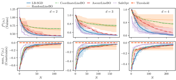
Figure 2: Accuracy (upper plots) and constraints (lower plots) of LB-SGD  and SafeOpt for $d=2,3,4$, averaged over $10$ samples. $t$ here is the amount of zeroth-order oracle calls. In these experiments, for LB-SGD  we decrease $\eta_{k+1}=0.7\eta_{k}$ gradually every $T_{k}=7$ steps with $n_{k}=[\frac{d}{2}]$ value measurements at each step. Already for $d=4$ LB-SGD  starts outperforming all BO-based methods on this problem in terms of the sample complexity. Best viewed in color.

Even for $d=4$, LB-SGD  is already notably more sample efficient compared to both SafeOpt and LineBO. Moreover, LB-SGD  significantly outperforms SafeOpt over computational cost and memory usage. It is well known that SafeOpt’s sample complexity and computational cost can exponentially depend on the dimensionality. In contrast, the complexity of LB-SGD depends on $d$ polynomially. The runtimes of the above experiments, in seconds, are shown in Table 2 and Figure 4.

$d$	2	3	4
SafeOpt (SafeOptSwarm)	4.289	114.406	212.514
LineBO	8.180	17.837	40.8
LB-SGD	0.429	0.895	0.781

Table 2: Average runtime dependence on dimensionality $d$ (in seconds). Importantly, the wall-clock time of LB-SGD remains roughly constant as we increase $d$, noting that we only increase the number of measurements per iteration, but not the number of iterations.

5.1.2 Non-convex objective and constraints

As a non-convex example, we consider the Rosenbrock function, a common benchmark for black-box optimization, with quadratic constraints. In particular, we consider the following problem

$$\min_{x\in\mathbb{R}^{d}}\sum_{i=1}^{d-1}100\|x_{i}-x_{i+1}\|^{2}-\|1-x_{i}\|^{2},$$

$$\text{s.t. }\|x\|^{2}\leq r_{1}^{2},\,\|x-\hat{x}\|^{2}\leq r_{2}^{2}.$$

We set $r_{1}=0.1$, $r_{2}=0.2$, $\hat{x}=[-0.05,\ldots,-0.05].$ The optimum of this problem is on the boundary of the constraint set. We show the comparison of LB-SGD  and SafeOpt on Figure 3.

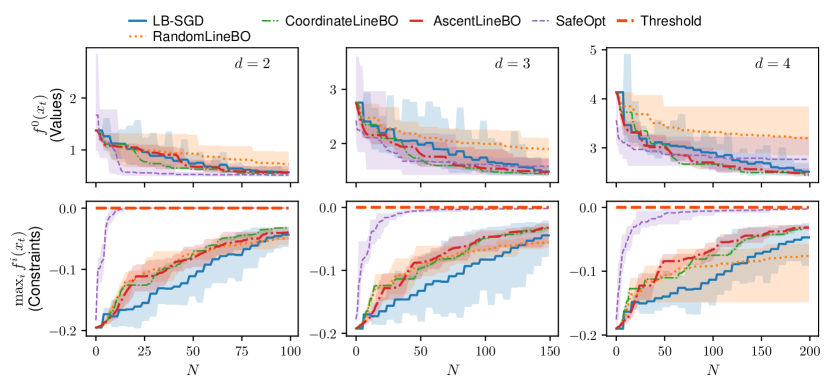
Figure 3: Accuracy and constraints of LB-SGD  and SafeOpt for $d=2,3,4$, averaged over $10$ samples. $t$ here is the amount of zeroth-order oracle calls. In these experiments, for LB-SGD  we decrease $\eta_{k+1}=0.7\eta_{k}$ gradually every $T_{k}=5$ steps with $n_{k}=d-1$ value measurements at each step. On this problem, for $d=4$ we observe that LB-SGD  performs better that SafeOpt, and comparable to LineBO. Best viewed in color.

Again, for $d=2$ we run SafeOpt, and for $d=3,4$ we run SafeOptSwarm. Here, on the constraints plot of SafeOpt and LineBO we again plot the highest value of the constraints over all points explored so far.

The run-times of LineBO and SafeOpt are demonstrated in Table 3 and Figure 4.

$d$	2	3	4
SafeOpt (SafeOptSwarm)	26.960	44.909	63.019
LineBO	7.584	10.593	13.293
LB-SGD	0.294	0.332	0.324

Table 3: Run-time (in seconds) as dependent on dimensionality $d$ (Rosenbrock benchmark).

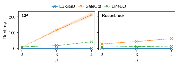
Figure 4: Run-times of LB-SGD  and SafeOpt for $d=2,3,4$, averaged over $10$ samples, in seconds. $t$ here is the amount of zeroth-order oracle calls. We can observe that LB-SGD  is a significantly cheaper approach in terms of the computational cost compared to both BO-based methods with growing dimensions.

Note that the second problem is easier for BO methods than the first one. It is related to the fact that in the first problem, the number of constraints (and therefore, the number of GPs) is higher and grows with dimensionality ($m=4,6,8$). In contrast, there are always only two constraints for the second problem. As one can see, our approach is significantly cheaper in computational time than SafeOpt. This is, of course, at the price of finding only a local minimum, not the global one.

5.1.3 Comparison with LineBO in higher dimensions

In higher dimensions, it is well known that SafeOpt is not tractable. Therefore, we compare our method only with LineBO (Kirschner et al., 2019). This method scales significantly better with dimensionality than the classical BO approaches. The method was demonstrated to be efficient in the unconstrained case and in cases where the solution lies in the interior of the constraint set. The authors proved the theoretical convergence in the unconstrained case and the safety of the iterations in the constrained case. However, in contrast to our method, this approach has a drawback that we discuss below. At each iteration, LineBO samples a direction (at random, an ascent direction of the objective, or a coordinate direction). Then it solves a 1-dimensional constrained optimization along this direction, using SafeOpt. After optimizing along this direction, it samples another direction starting from the current point. The drawback of this approach is that when the solution is on the boundary, LineBO might get stuck on the wrong point on the boundary. In such a case, it might be difficult for it to find a safe direction of improvement too close to the boundary. See Figure 5 for the illustration of this potential problem. Furthermore, the higher dimension, the harder it is to sample a suitable direction.

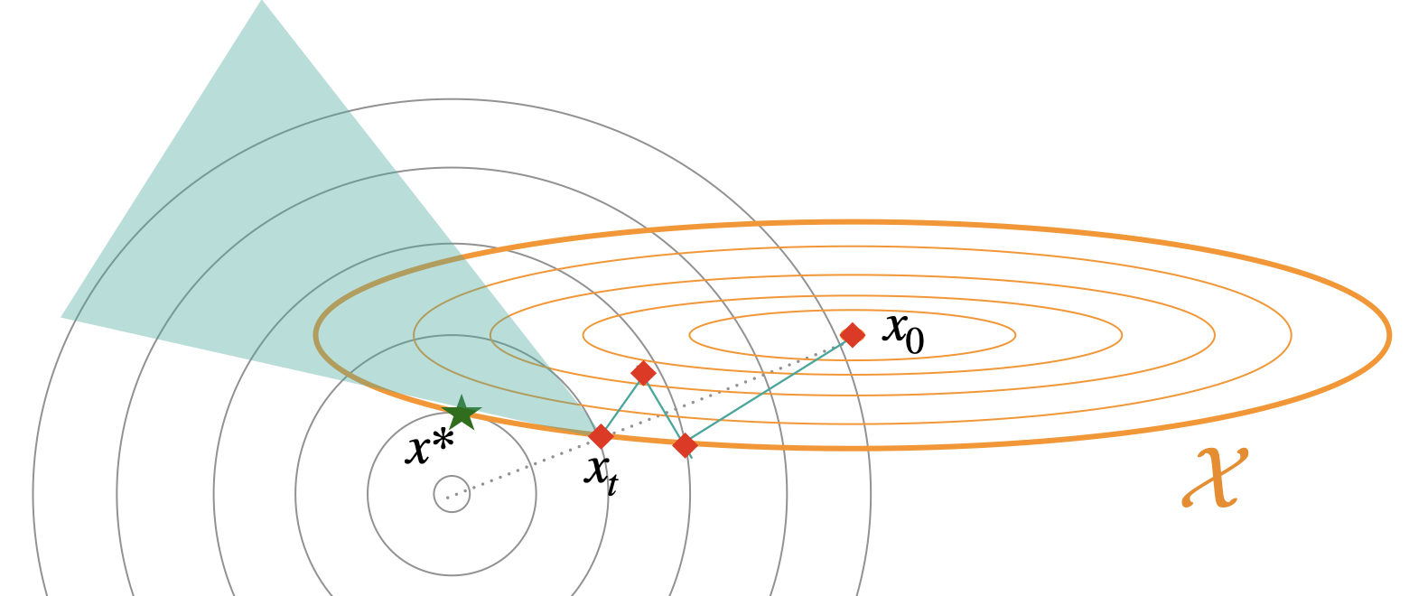
Figure 5: Illustration of the LineBO behavior. At point $x_{t}$ not every direction allows the safe improvement (only the directions lying in the green sector). Therefore, the LineBO method might get stuck sampling the wrong directions. On this example, the closer to the solution, the narrower is the improvement sector.

We demonstrate that empirically in application to the following problem:

$$\min_{x\in\mathbb{R}^{d}}-\text{exp}^{-4\|x\|^{2}},$$ (34)

$$\text{s.t. }\langle x-\hat{x},A(x-\hat{x})\rangle\leq r^{2},$$ (35)

with $r=0.5$ and $A=\text{diag}(3,1.2,\ldots,1.2).$ On Figure 6 we demonstrate the comparison of LineBO and LB-SGD  methods on the above problem for dimensionalities $d=2,10,20$.

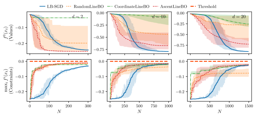
Figure 6: Accuracy and constraints of LB-SGD  and SafeRandomLineBO for $d=2,10,20$, averaged over $10$ samples. $t$ here is the amount of zeroth-order oracle calls. In these experiments, for LB-SGD  we decrease $\eta_{k+1}=0.85\eta_{k}$ gradually every $T_{k}=3$ steps with $n_{k}=[\frac{d+1}{2}]$ value measurements at each step.

We report the run-times in Table 4.

$d$	2	10	20
LB-SGD	0.828	2.186	2.676
LineBO	12.883	298.097	1038.459

Table 4: Runtime (in seconds) dependence on dimensionality $d$ on the negative Gaussian minimization benchmark. We can observe that LineBO is significantly more expensive in computational cost (for the same number of queried points).

To compare, in the case when the solution is in the interior of the constraint set achieved by setting $r=10$ (that is, if the constraints do not influence the solution), the LineBO approach does not have this issue and can still be very efficient (see Figure 7).

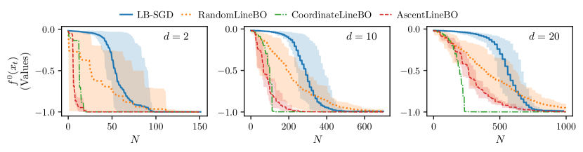
Figure 7: Accuracy and constraints of LB-SGD  and SafeRandomLineBO for $d=2,10,20$, averaged over $10$ samples. $t$ here is the amount of zeroth-order oracle calls. In these experiments, for LB-SGD  we decrease $\eta_{k+1}=0.85\eta_{k}$ gradually every $T_{k}=3$ steps with $n_{k}=[\frac{d+1}{2}]$ value measurements at each step.

5.2 LB-SGD for safe reinforcement learning

We previously showed LB-SGD performance on smaller scale, classical black box benchmark problems. In this part, we showcase how LB-SGD scales to more complex, high-dimensional domains arising in RL. We consider the “Safety Gym” (Ray et al., 2019) benchmark suite designed to evaluate safe RL approaches on constrained Markov decision processes (CMDP). In Safety Gym, a robot needs to reach a goal area while avoiding obstacles on the way. Navigation is done by observing first-person-view of the robot.

5.2.1 Problem statement

Constrained Markov decision processes

The problem of safe reinforcement learning can be viewed as finding a policy that solves a constrained Markov decision process (Altman, 1999). Briefly, we define a discrete-time episodic CMDP as a tuple $\left(\mathcal{S},\mathcal{A},\rho,P,R,\gamma,\mathcal{C}\right)$. At each time step $\tau\in\{0,\dots,\mathrm{T}\}$, an agent observes a state $s_{\tau}\in\mathcal{S}$. The initial state $s_{0}$ is determined according to some unknown distribution $\rho(s_{0})$ such that $s_{0}\sim\rho(s_{0})$. Given a state, the agent decides what action $a_{\tau}\in\mathcal{A}$ to take next. Then, an unknown transition density $P:\mathcal{S}\times\mathcal{A}\times\mathcal{S}\rightarrow\left[0,1\right]$, $s_{\tau+1}\sim P(\cdot|s_{\tau},a_{\tau})$ generates a new state. $R:\mathcal{S}\times\mathcal{A}\rightarrow\mathbb{R}$ is a reward function that generates an immediate reward signal observed by the agent. The discount factor $\gamma\in(0,1]$ weighs the importance of immediate rewards compared to future ones. Lastly, $\mathcal{C}=\left\{c^{i}:\mathcal{S}\times\mathcal{A}\rightarrow\mathbb{R}\bigm{|}i\in\left[m\right]\right\}$ is a set of immediate cost signals that the agent observes alongside the reward. The goal is to find a policy $\pi:\mathcal{S}\times\mathcal{A}\rightarrow\left[0,1\right]$ that solves the constrained problem:

$$\max_{\pi} \;\underbrace{\mathbb{E}\left[\sum_{\tau}\gamma^{\tau}R(s_{\tau},a_{\tau})\right]}_{-f^{0}(x)} \text{s.t. }\;\underbrace{\mathbb{E}\left[\sum_{\tau}\gamma^{\tau}c^{i}(s_{\tau},a_{\tau})\right]-d^{i}}_{f^{i}(x)}\leq 0\;\forall i\in[m].$$ (36)

In the above, $d^{i},i\in[m]$ are predefined threshold values for the expected discounted return of costs. Note that we take the expectation with respect to all stochasticity induced by the CMDP and policy.

On-policy methods as black-box optimization problems

A typical recipe for solving CMDPs at scale is to parameterize the policy with parameters $x$ and use on-policy methods. On-policy methods use Monte-Carlo sampling to sample trajectories from the environment, evaluate the policy, and finally update it (Chow et al., 2015; Achiam et al., 2017; Ray et al., 2019). By using Monte-Carlo, these methods compute unbiased estimates of the constraints, objective and their gradients (e.g., via REINFORCE, cf. Sutton et al., 2000), equivalently to the assumptions in Section 2.1. In particular, the process of sampling trajectories from the CMDP and averaging them to estimate the objective and constraints in Equation 36 is equivalent to querying $f^{0}(x)$ and $f^{i}(x),i\in[m]$ and gives rise to a first-order, stochastic and unbiased oracle. However, without deliberately enforcing $x_{t}\in\mathcal{X}\ \forall t\in\{0,\dots,T\}$, these methods may use an unsafe policy during learning.

Solving CMDPs with LB-SGD

Another shortcoming of the previously mentioned algorithms is that using only Monte-Carlo sampling often leads to high variance estimates of $f^{0}(x)$ and $f^{i}(x)$ (Schulman et al., 2015). To reduce this variance, one is typically required to take an abundant number of queries of $f^{0}(x)$ and $f^{i}(x)$, making the aforementioned algorithms sample-inefficient. One way to improve sample efficiency, is to learn a model of the CMDP, and query it (instead of the real CMDP) to have approximations of $f^{0}(x)$ and $f^{i}(x)$. This allows us to trade off the high variance and sample inefficiency with some bias introduced my model errors. By making this compromise, model-based methods empirically exhibit improved sample efficiency compared to the previously mentioned on-policy methods (Deisenroth and Rasmussen, 2011; Chua et al., 2018; Hafner et al., 2021). Motivated by this insight, we use LAMBDA (As et al., 2022), a recent model-based approach for solving CMDPs. In short, LAMBDA learns the transition density $P$ from image observations, and uses this learned model to try to find an optimal policy. To accommodate the complexity of learning a policy from a high dimensional input such as images, LAMBDA requires $\sim$588400 parameters to parameterize the policy. This allows us to demonstrate LB-SGD’s ability to scale to problems with large dimensionality. To solve Equation 36, LAMBDA queries approximations of $f^{0}(x),f^{i}(x)$ by using its model of the CMDP together with its policy to sample model-generated, on-policy trajectories. As described before, these model-generated trajectories are subject to model errors which in turn makes the estimation of the objective and constraints biased. As a result, the assumptions in Section 2.1 do not necessarily, hold as in this case, the oracle is first-order, stochastic but biased. Nevertheless, this biasedness is subject only to LAMBDA’s model inaccuracies, so LB-SGD can still produce safe policies with high utility, as we empirically show in the following section. As et al. (2022) use the “Augmented Lagrangian” (Nocedal and Wright, 2006) to turn the constrained problem into an unconstrained one. However, by using the Augmented Lagrangian, $x_{t}$ are generally infeasible throughout training, even if $x_{0}\in\mathcal{X}$. Therefore, we use LB-SGD instead and empirically show that by using it we get $x_{t}\in\mathcal{X}\;\forall t\in\{0,\dots,T\}$.

5.2.2 Experiments

Addressing the assumptions

Let us briefly discuss the assumptions in Section 2 and explicitly state which of them do not hold. Oracle. As mentioned before, we cannot guarantee the assumptions in Section 2.1. LAMBDA uses neural networks to model the transition density and to learn an approximation of the objective and constraints. For this reason, the assumption on unbiased zeroth-order queries, and assumptions of sub-Gaussian oracles do not hold. Smoothness. By choosing ELU activation function (Clevert et al., 2015) we ensure the smoothness of our approximation of the objective and constraints. MFCQ. In general, similarly to the assumptions on the oracle, this cannot be guaranteed. However, in our experiments, the CMDP is defined to have only one constraint ($m=1$) so this assumption is satisfied by definition. Safe initial policy. This assumption exists in a large body of previous work (Berkenkamp et al., 2017; Koller et al., 2018; Wabersich and Zeilinger, 2021). Yet, it is not always clear how to design such a policy a-priori. In the following, we propose an experimental protocol in which this assumption empirically holds.

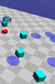
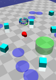
Figure 8: In Safety Gym, a robot should navigate to a goal area (green circle), while avoiding all other objects (turquoise and blue). The robot on the right picture should arrive to a smaller goal region, making navigation harder.

Experiment protocol

To ensure LB-SGD starts from a safe policy, we warm-start it with a policy that was trained on a similar, but easier task. Specifically, we follow a similar experimental setup as As et al. (2022) but first train the agent with LAMBDA on a task in which the goal area is larger, as shown in Figure 8. We use the policy parameters of the trained agent as a starting point for LB-SGD on a harder task, in which the goal area is smaller. As we later show, this allows the agent to start the second stage with a safe but sub-optimal policy. We verify this setup with all three available robots of the Safety-Gym benchmark suite (Ray et al., 2019), each run with 5 different random seeds. For our implementation, please see https://github.com/lasgroup/lbsgd-rl.

Results

We first validate our experimental setup. In Figure 9 we show that by using either LB-SGD or the Augmented Lagrangian in the first stage, and not updating the policy in the second stage, LAMBDA’s policy is safe but sub-optimal. With this, we empirically confirm the safe initial policy assumption on the second stage of training. Further, given such a policy, we compare LB-SGD with the Augmented Lagrangian on the second stage. In Figure 10 we demonstrate how the Augmented Lagrangian needs to “re-learn” a new value for the Lagrange multiplier and therefore fails to transfer safely to the harder task. However, by using LB-SGD, the agent is able to maintain safety after transitioning to the harder task. It is important to note that this safe transfer comes at the cost of limited exploration. As shown in Figures 9 and 10, LB-SGD finds slightly less performant policies compared to the Augmented Lagrangian. In Figure 10 we also compare with the classical constrained policy optimization (CPO) algorithm (Achiam et al., 2017) following the implementation in https://github.com/lasgroup/jax-cpo as a baseline. CPO is a model-free method and hence requires much more environment interactions. Therefore, we only show the final level CPO reaches after 10 million environment steps.

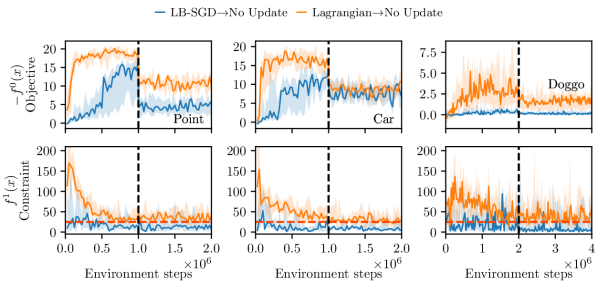
Figure 9: Across all different robots of the Safety Gym suite, LAMBDA with LB-SGD and the Augmented Lagrangian transfer well to the second stage in terms of safety. Since we do not update the policy, LAMBDA fails to reach the same task performance on the second stage, as expected. Shaded areas represent the the 5% and 95% percentiles of 5 different random seeds.

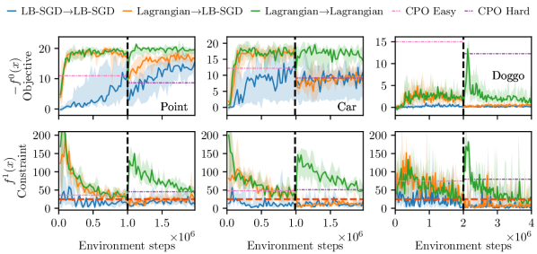
Figure 10: LAMBDA with LB-SGD transfers safely to the second task. The main trade-off, however, is the lower asymptotic performance of LB-SGD. Conversely, Lagrangian $\rightarrow$ Lagrangian fails transfer safely as the constraints with all robots rapidly grow when the new task is revealed (as shown by the vertical dashed black line). CPO Easy and CPO Hard correspond to CPO’s performance on the easier task (larger goal size) and the harder task (smaller goal size). We train CPO on each task separately and show its performance at convergence, i.e., after $10\times 10^{6}$ interaction steps for the “Point” and “Car” robots and $100\times 10^{6}$ for the “Doggo” robot. As shown, while CPO achieves reasonable performance, it fails to satisfy the constraints in all tasks and all robots, as previously reported by Ray et al. (2019).

6 Conclusion

In this paper, we addressed the problem of sample and computationally efficient safe learning. We proposed an approach based on logarithmic barriers, which we optimize using SGD with adaptive step sizes. We analytically proved its safety during the learning and analyzed the convergence rates for non-convex, convex, and strongly-convex problems. We empirically demonstrated the performance of our method in comparison with other existing methods. We show that 1) its sample and computational complexity scale efficiently to high dimensions, and; 2) it keeps optimization iterates within the feasible set with high probability. Additionally, we demonstrate the efficiency of the log barrier approach for high-dimensional constrained reinforcement learning problems.

While not requiring to explicitly specify a prior (in the Bayesian sense, as considered in safe Bayesian optimization), our method does involve hyper-parameters such as $\eta_{0}$, $\eta$-decrease rate parameter $\omega$, amount of steps per episode $T_{k}$, and exhibits sensitivity to the noise. Also, in the non-convex case, it can converge only to a local minimum, as any other descent optimization approach. However, it is easy to implement and has efficient computational performance due to cheap updates. Therefore, LB-SGD is better suited to problems of high scale.

For future work, it would be exciting to take the best of both worlds and combine the BO approaches that allow us to build and use a global model with our simple and cheap safe descent approach based on log barriers.

7 Acknowledgements

We thank the support of Swiss National Science Foundation, under the grant SNSF 200021_172781, the Swiss National Science Foundation under NCCR Automation, grant agreement 51NF40 180545, and European Research Council (ERC) under the European Union’s Horizon 2020 research and innovation programme grant agreement No 815943.

Appendix A Additional proofs

First, on Figure 11 we show how various theorems and lemmas relate to each other throughout our paper.

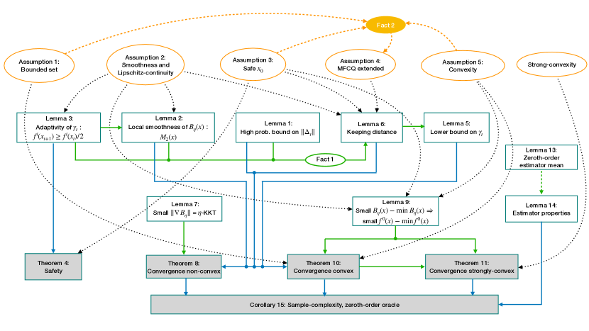
Figure 11: Relations of our theoretical results.

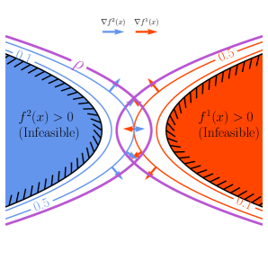
Figure 12: Illustration of extended MFCQ.

A.1 MFCQ

Let $x^{*}$ be a local minimizer of constrained problem (P), and let $\mathcal{I}(x^{*}):=\{i\in[m]:f^{i}(x^{*})=0\}$ denote the set of active constraints at $x^{*}$. Then, the classic MFCQ is satisfied at $x^{*}$ if there exists $s\in\mathbb{R}^{d}$ such that $\langle s,\nabla f^{i}(x^{*})\rangle<0$ for all $i\in\mathcal{I}(x^{*}).$

On Figure 12, for the point in the middle, both constraints are $\rho$-almost active. Note that at this point, no descent direction exists for both constraints since their gradients are pointing to the opposite directions. That is, this set does not satisfy the extended MFCQ with the given $\rho>0$.

A.2 Proof of Lemma 1

Proof  Using the triangle inequality, we get

$$\|\Delta_{t}\| =\|g_{t}-\nabla B_{\eta}(x_{t})\|$$

$$=\left\|G^{0}_{n}(x_{t})-\nabla f^{0}(x_{t})+\sum_{i=1}^{m}\left[\eta G^{i}_{n}(x_{t})\left(\frac{1}{\bar{\alpha}_{t}^{i}}-\frac{1}{\alpha_{t}^{i}}\right)+\eta(G^{i}_{n}(x_{t})-\nabla f^{i}(x_{t}))\frac{1}{\alpha_{t}^{i}}\right]\right\|$$

$$\leq\left\|G^{0}_{n}(x_{t})-\nabla f^{0}(x_{t})\right\|+\sum_{i=1}^{m}\left[\eta\left\|G^{i}_{n}(x_{t})\right\|\left(\frac{1}{\bar{\alpha}_{t}^{i}}-\frac{1}{\alpha_{t}^{i}}\right)+\frac{\eta}{\alpha_{t}^{i}}\left\|G^{i}_{n}(x_{t})-\nabla f^{i}(x_{t}))\right\|\right].$$

With high probability, we know $\|G^{i}_{n}(x_{t})\|\leq L_{i}$, and from the sub-Gaussian property we have:

$$\mathbb{P}\left\{\left\|G^{i}_{n}(x_{t})-\nabla f^{i}(x_{t})\right\|\leq\hat{b}_{i}+\hat{\sigma}_{i}(n)\sqrt{\ln\frac{1}{\delta}}\right\}\geq 1-\delta$$

$$\mathbb{P}\left\{\left|\alpha_{t}^{i}-\bar{\alpha}_{t}^{i}\right|\leq\sigma_{i}(n)\sqrt{\ln\frac{1}{\delta}}\right\}\geq 1-\delta,$$

from what we conclude:

$$\mathbb{P}\left\{\|\Delta_{t}\|\leq\hat{b}_{0}+\hat{\sigma}_{0}(n)\sqrt{\ln\frac{1}{\delta}}+\sum_{i=1}^{m}\frac{\eta}{\bar{\alpha}_{t}^{i}}\left(\hat{b}_{i}+\hat{\sigma}_{i}(n)\sqrt{\ln\frac{1}{\delta}}\right)+\sum_{i=1}^{m}L_{i}\frac{\eta}{\alpha_{t}^{i}\bar{\alpha}_{t}^{i}}\sigma_{i}(n)\sqrt{\ln\frac{1}{\delta}}\right\}\geq 1-\delta.$$

 

A.2.1 Bias

Proof  Using $\mathbb{E}[XY]\leq\sqrt{\mathbb{E}[X^{2}]\mathbb{E}[Y^{2}]}$, we get

$$\|\mathbb{E}\Delta_{t}\| =\|\mathbb{E}[g_{t}-\nabla B_{\eta}(x_{t})]\|$$

$$\leq\left\|\mathbb{E}[G^{0}(x_{t})-\nabla f^{0}(x_{t})]+\sum_{i=1}^{m}\mathbb{E}\left[\eta G^{i}(x_{t})\left(\frac{1}{\bar{\alpha}_{t}}-\frac{1}{\alpha_{t}}\right)+\eta(G^{i}(x_{t})-\nabla f^{i}(x_{t}))\frac{1}{\alpha_{t}}\right]\right\|$$

$$=\left\|\sum_{i=1}^{m}\mathbb{E}\left[\eta G^{i}(x_{t})\left(\frac{1}{\bar{\alpha}_{t}}-\frac{1}{\alpha_{t}}\right)\right]\right\|+\hat{b}^{0}_{t}+\sum_{i=1}^{m}\frac{\eta}{\alpha_{t}^{i}}\hat{b}^{i}_{t}$$

$$\leq\sum_{i=1}^{m}\mathbb{E}\left[\left\|\eta G^{i}(x_{t})\left(\frac{1}{\bar{\alpha}_{t}^{i}}-\frac{1}{\alpha_{t}^{i}}\right)\right\|\right]+\hat{b}^{0}_{t}+\sum_{i=1}^{m}\frac{\eta}{\alpha_{t}^{i}}\hat{b}^{i}_{t}$$

$$\leq\sum_{i=1}^{m}\sqrt{\mathbb{E}[\eta^{2}\|G^{i}(x_{t})\|^{2}]\mathbb{E}\left[\frac{1}{(\bar{\alpha}_{t}^{i})^{4}}\|\alpha_{t}^{i}-\bar{\alpha}_{t}^{i}\|^{2}\right]}+\hat{b}^{0}_{t}+\sum_{i=1}^{m}\frac{\eta}{\alpha_{t}^{i}}\hat{b}^{i}_{t}$$

$$\leq\sum_{i=1}^{m}\frac{\eta L_{i}\sigma_{t}}{(\alpha_{t}^{i})^{2}}+\hat{b}^{0}_{t}+\sum_{i=1}^{m}\frac{\eta}{\alpha_{t}^{i}}\hat{b}^{i}_{t},$$

 

A.3 Proof of the adaptivity

Proof  For adaptivity, we require

$$f^{i}(x_{t+1})\leq\frac{f^{i}(x_{t})}{2}.$$

Using $M_{i}$-smoothness, we can bound the $i$-th constraint growth:

$$f^{i}(x_{t+1}) \leq f^{i}(x_{t})+\langle\nabla f^{i}(x_{t}),x_{t+1}-x_{t}\rangle+\frac{M_{i}}{2}\|x_{t}-x_{t+1}\|^{2}$$

$$=f^{i}(x_{t})-\gamma_{t}\langle\nabla f^{i}(x_{t}),g_{t}\rangle+\gamma_{t}^{2}\frac{M_{i}}{2}\|g_{t}\|^{2}$$

That is, the condition on $\gamma_{t}$ for adaptivity (and safety) we can formulate by

$$-\gamma_{t}\langle\nabla f^{i}(x_{t}),g_{t}\rangle+\gamma_{t}^{2}\frac{M_{i}}{2}\|g_{t}\|^{2}\leq\frac{-f^{i}(x_{t})}{2}=\frac{\alpha_{t}^{i}}{2}.$$

By carefully rewriting the above inequality without strengthening it, we get

$$\gamma_{t}^{2}\frac{M_{i}}{2}\|g_{t}\|^{2}-\gamma_{t}\langle\nabla f^{i}(x_{t}),g_{t}\rangle\pm\frac{1}{2M_{i}}\frac{\langle\nabla f^{i}(x_{t}),g_{t}\rangle^{2}}{\|g_{t}\|^{2}}\leq\frac{\alpha_{t}}{2}$$

$$\left(\gamma_{t}\|g_{t}\|-\frac{\langle\nabla f^{i}(x_{t}),g_{t}\rangle}{M_{i}\|g_{t}\|}\right)^{2}\leq\frac{\alpha_{t}}{M_{i}}+\frac{\langle\nabla f^{i}(x_{t}),g_{t}\rangle^{2}}{M_{i}^{2}\|g_{t}\|^{2}}$$

Using the quadratic inequality solution, we obtain the following sufficient bound on the adaptive $\gamma_{t}:$

$$\gamma_{t}\|g_{t}\|\leq\frac{\langle\nabla f^{i}(x_{t}),g_{t}\rangle}{M_{i}\|g_{t}\|}+\sqrt{\frac{\alpha_{t}}{M_{i}}+\frac{\langle\nabla f^{i}(x_{t}),g_{t}\rangle^{2}}{M_{i}^{2}\|g_{t}\|^{2}}}=(*)$$

Then, we can rewrite this expression of the right part as follows:

$$(*) =\sqrt{\frac{\langle\nabla f^{i}(x_{t}),g_{t}\rangle^{2}}{M_{i}^{2}\|g_{t}\|^{2}}+\frac{\alpha^{i}_{t}}{M_{i}}}+\frac{\langle\nabla f^{i}(x_{t}),g_{t}\rangle}{M_{i}\|g_{t}\|}=\sqrt{\frac{\alpha_{t}^{i}}{M_{i}}}\left(\sqrt{\frac{\langle\nabla f^{i}(x_{t}),g_{t}\rangle^{2}}{M_{i}\alpha_{t}^{i}\|g_{t}\|^{2}}+1}+\frac{\langle\nabla f^{i}(x_{t}),g_{t}\rangle}{\sqrt{M_{i}\alpha_{t}^{i}}\|g_{t}\|}\right)$$

$$=\sqrt{\frac{\alpha_{t}^{i}}{M_{i}}}\frac{1}{\sqrt{\frac{\langle\nabla f^{i}(x_{t}),g_{t}\rangle^{2}}{M_{i}\alpha_{t}^{i}\|g_{t}\|^{2}}+1}-\frac{\langle\nabla f^{i}(x_{t}),g_{t}\rangle}{\sqrt{M_{i}\alpha_{t}^{i}}\|g_{t}\|}}=\frac{\alpha_{t}^{i}}{\sqrt{\frac{\langle\nabla f^{i}(x_{t}),g_{t}\rangle^{2}}{\|g_{t}\|^{2}}+M_{i}\alpha_{t}^{i}}-\frac{\langle\nabla f^{i}(x_{t}),g_{t}\rangle}{\|g_{t}\|}}$$

$$=\frac{\alpha_{t}^{i}}{\sqrt{(\theta_{t}^{i})^{2}+M_{i}\alpha_{t}^{i}}-\theta_{t}^{i}}$$

Therefore, the condition $\gamma_{t}\leq\min_{i\in[1,m]}\left\{\frac{\alpha_{t}^{i}}{\sqrt{(\theta_{t}^{i})^{2}+M_{i}\alpha_{t}^{i}}-\theta_{t}^{i}}\right\}\frac{1}{\|g_{t}\|}$ is sufficient for $f^{i}(x_{t+1})\leq\frac{f^{i}(x_{t})}{2}.$ Using the Cauchy-Schwartz inequality, we can simplify this condition (but making it more conservative):

$$(*)\geq\frac{\alpha_{t}^{i}}{\sqrt{(\theta_{t}^{i})^{2}+\alpha_{t}M_{i}}+|\theta_{t}^{i}|}\geq\frac{\alpha^{i}_{t}}{2|\theta_{t}^{i}|+\sqrt{\alpha_{t}^{i}M_{i}}}.$$

 

A.4 Proof of the local smoothness

Proof  Let us define the hessian of the log-barrier $B_{\eta}(x)$ by $H_{B}(y)$ at the region $Y_{t}$ around $x_{t}$ such that $Y_{t}:=\{y\in\mathbb{R}^{d}|y=x_{t}-ug_{t},u\in[0,\gamma_{t}]\}.$ Note that by definition of the log barrier, the hessian of it at the point $y\in Y_{t}$ is given by

$$H_{B}(y)=\nabla^{2}B_{\eta}(y)=\nabla^{2}f^{0}(y)+\sum_{i=1}^{m}\eta\frac{\nabla^{2}f^{i}(y)}{-f^{i}(y)}+\sum_{i=1}^{m}\eta\frac{\nabla f^{i}(y)\nabla f^{i}(y)^{T}}{(-f^{i}(y))^{2}}.$$

From the above and the fact that for any $y\in Y_{t}$ we have $-f^{i}(y)\geq 0.5\alpha_{t}$, we get

$$|g_{t}^{T}H_{B}(y)g_{t}| \leq M_{{\color[rgb]{0,0,0}0}}\|g_{t}\|^{2}+\eta\sum_{i=1}^{m}\frac{M_{i}}{0.5\alpha_{t}^{i}}\|g_{t}\|^{2}+\eta\sum_{i=1}^{m}\frac{(\nabla f^{i}(y)^{T}g_{t}/\|g_{t}\|)^{2}}{(0.5\alpha_{t}^{i})^{2}}\|g_{t}\|^{2}$$

$$\leq\|g_{t}\|^{2}\left(M_{{\color[rgb]{0,0,0}0}}+\eta\sum_{i=1}^{m}\frac{M_{i}}{0.5\alpha_{t}^{i}}+\eta\sum_{i=1}^{m}\frac{\langle\nabla f^{i}(y),g_{t}\rangle^{2}/\|g_{t}\|^{2}}{(0.5\alpha_{t}^{i})^{2}}\right)$$

$$\leq\|g_{t}\|^{2}\left(M_{{\color[rgb]{0,0,0}0}}+2\eta\sum_{i=1}^{m}\frac{M_{i}}{\alpha_{t}^{i}}+4\eta\sum_{i=1}^{m}\frac{\langle\nabla f^{i}(y),g_{t}\rangle^{2}}{(\alpha_{t}^{i})^{2}\|g_{t}\|^{2}}\right).$$

Thus,

$$M_{2}(x_{t})=M_{{\color[rgb]{0,0,0}0}}+2\eta\sum_{i=1}^{m}\frac{M_{i}}{\alpha_{t}^{i}}+4\eta\sum_{i=1}^{m}\frac{\langle\nabla f^{i}(y),g_{t}\rangle^{2}}{{\color[rgb]{0,0,0}(\alpha_{t}^{i})}^{2}\|g_{t}\|^{2}}.$$

Note that $\nabla f^{i}(y)$ is unknown, therefore we have to bound it based on $\nabla f^{i}(x_{t}).$ Observe that

$$\langle\nabla f^{i}(y),g_{t}\rangle^{2}$$ (37)

$$=\langle\nabla f^{i}(x_{t}),g_{t}\rangle^{2}+\langle\nabla f^{i}(y)-\nabla f^{i}(x_{t}),g_{t}\rangle^{2}+2\langle\nabla f^{i}(x_{t}),g_{t}\rangle\langle\nabla f^{i}(x_{t+1})-\nabla f^{i}(x_{t}),g_{t}\rangle.$$

Using the $M_{i}$-smoothness of $f^{i}(x)$ we get:

$$\|\nabla f^{i}(x_{t})-\nabla f^{i}(y)\|\leq M_{i}\|x_{t}-y\|\leq M_{i}\gamma_{t}\|g_{t}\|.$$

Recall that we choose the step-size such that:

$$\gamma_{t}\leq\min_{i\in[m]}\left\{\frac{\alpha^{i}_{t}}{2|\theta_{t}|+\sqrt{\alpha_{t}^{i}M^{i}}}\right\}\frac{1}{\|g_{t}\|_{2}}.$$

Hence,

$$\|\nabla f^{i}(x_{t})-\nabla f^{i}(y)\|\leq M_{i}\|x_{t}-y\|\leq\frac{M_{i}\alpha^{i}_{t}}{2|\theta_{t}|+\sqrt{\alpha_{t}^{i}M_{i}}}\leq\frac{M_{i}\alpha^{i}_{t}}{\sqrt{\alpha_{t}^{i}M_{i}}}=\sqrt{\alpha_{t}^{i}M_{i}}.$$

Then, using Equation 37 and $\langle\nabla f^{i}(x_{t}),g_{t}\rangle^{2}=(\theta_{t}^{i})^{2}\|g_{t}\|^{2}$ we get:

$$\langle\nabla f^{i}(y),g_{t}\rangle^{2} \leq|\theta_{t}^{i}|^{2}\|g_{t}^{i}\|^{2}+\alpha_{t}^{i}M_{i}\|g_{t}^{i}\|^{2}+2|\theta_{t}^{i}|\sqrt{\alpha_{t}^{i}M^{i}}\|g_{t}^{i}\|^{2}$$ (38)

$$\leq 2|\theta_{t}^{i}|^{2}\|g_{t}^{i}\|^{2}+2\alpha_{t}^{i}M^{i}\|g_{t}^{i}\|^{2}.$$ (39)

The above inequality is due to the fact that $a^{2}+2ab+b^{2}\leq 2a^{2}+2b^{2}$. Thus, we finally obtain

$$M_{2}(x_{t}) =M_{0}+2\eta\sum_{i=1}^{m}\frac{M_{i}}{\alpha^{i}_{t}}+4\eta\sum_{i=1}^{m}\frac{2|\theta_{t}^{i}|^{2}\|g_{t}^{i}\|^{2}+2\alpha_{t}^{i}M^{i}\|g_{t}^{i}\|^{2}}{(\alpha^{i}_{t})^{2}\|g_{t}\|^{2}}$$

$$=M_{0}+10\eta\sum_{i=1}^{m}\frac{M_{i}}{\alpha^{i}_{t}}+8\eta\sum_{i=1}^{m}\frac{(\theta_{t}^{i})^{2}}{(\alpha^{i}_{t})^{2}}.$$

 

A.5 Proof of Fact 1

Fact 1

Let Assumptions 2, 3 hold, and Assumption 4 hold with $\rho\geq\eta$, and let $\hat{\sigma}_{i}(n)\leq\frac{(\alpha_{t}^{i})^{2}L}{2\eta\sqrt{\ln\frac{1}{\delta}}}$, $\hat{b}_{i}\leq\frac{(\alpha_{t}^{i})^{2}L}{2\eta}$, and $\sigma_{i}(n)\leq\frac{\alpha_{t}^{i}}{2\sqrt{\ln\frac{1}{\delta}}}$. If at iteration $t$ we have $\min_{i\in[m]}\alpha_{t}^{i}\leq\bar{c}\eta$ with $\bar{c}:=\frac{l}{L}\frac{1}{2m+1}$, then, for the next iteration $t+1$ we get $\prod_{i\in\mathcal{\mathcal{I}}}\alpha_{t+1}^{i}\geq\prod_{i\in\mathcal{\mathcal{I}}}\alpha_{t}^{i}$ for any $\mathcal{I}:\mathcal{I}_{t}\subseteq\mathcal{I}$ with $\mathcal{I}_{t}:=\{i\in[m]:\alpha_{t}^{i}\leq\eta\}$.

Proof  Using the local smoothness of the log barrier, we can see:

$$\eta\sum_{i\in\mathcal{I}_{t}}-\log\alpha_{t+1}^{i} \leq\eta\sum_{i\in\mathcal{I}_{t}}-\log\alpha_{t}^{i}-\gamma_{t}\langle\eta\sum_{i\in\mathcal{I}_{t}}\frac{\nabla f^{i}(x_{t})}{\alpha^{i}_{t}},g_{t}\rangle+\frac{M_{2}(x_{t})}{2}\gamma_{t}^{2}\|g_{t}\|^{2}$$

$$\leq\eta\sum_{i\in\mathcal{I}_{t}}-\log\alpha_{t}^{i}+\gamma_{t}\left(-\langle\eta\sum_{i\in\mathcal{I}_{t}}\frac{\nabla f^{i}(x_{t})}{\alpha^{i}_{t}},g_{t}\rangle+\frac{1}{2}\|g_{t}\|^{2}\right)$$

$$=\eta\sum_{i\in\mathcal{I}_{t}}-\log\alpha_{t}^{i}+\frac{\gamma_{t}\eta^{2}}{2}\left(2\langle A,A+B\rangle+\|A+B\|^{2}\right)$$

$$=\eta\sum_{i\in\mathcal{I}_{t}}-\log\alpha_{t}^{i}+\frac{\gamma_{t}\eta^{2}}{2}\left(\|B\|^{2}-\|A\|^{2}\right),$$ (40)

where $g_{t}=A+B$, with $A:=\sum_{i\in\mathcal{I}_{t}}\frac{\nabla f^{i}(x_{t})}{\alpha_{t}^{i}}$ and $B:=\frac{g_{t}}{\eta}-\sum_{i\in\mathcal{I}_{t}}\frac{\nabla f^{i}(x_{t})}{\alpha_{t}^{i}}$. Using Assumption 4 we obtain a lower bound on $\|A\|$:

$$\|A\|=\left\|\sum_{i\in\mathcal{I}_{t}}\frac{\nabla f^{i}(x_{t})}{\alpha_{t}^{i}}\right\| \geq\langle\sum_{i\in\mathcal{I}_{t}}\frac{\nabla f^{i}(x_{t})}{\alpha_{t}^{i}},s_{x}\rangle\geq\sum_{i\in\mathcal{I}_{t}}\frac{\langle\nabla f^{i}(x_{t}),s_{x}\rangle}{\alpha_{t}^{i}}\geq\sum_{i\in\mathcal{I}_{t}}\frac{l}{\alpha_{t}^{i}}.$$ (41)

The second part $\|B\|$ we can upper bound with high probability $1-\delta$ using the definition of $\mathcal{I}_{t}$ as follows (since $\forall\alpha_{t}^{j}\notin\mathcal{I}_{t}$ we have $\alpha_{t}^{j}\geq\eta$, therefore $\bar{\alpha}_{t}^{j}\geq\eta/2$ for $\sigma_{i}(n)\leq\frac{\alpha_{t}^{i}}{2\sqrt{\ln\frac{1}{\delta}}}$):

$$\|B\| =\left\|\frac{G^{0}_{n}(x_{t},\xi_{t})}{\eta}+\sum_{j\notin\mathcal{I}_{t}}\frac{G^{j}_{n}(x_{t},\xi_{t})}{\bar{\alpha}_{t}^{j}}+\sum_{i\in\mathcal{I}_{t}}\frac{G^{i}_{n}(x_{t},\xi_{t})}{\bar{\alpha}_{t}^{i}}-\sum_{i\in\mathcal{I}_{t}}\frac{\nabla f^{i}(x_{t})}{\alpha_{t}^{i}}\right\|$$

$$\leq\frac{\max_{i}\|G^{i}_{n}(x_{t},\xi_{t})\|}{\eta}\left(1+2(m-|\mathcal{I}_{t}|)\right)+\sum_{i\in\mathcal{I}_{t}}\left(\frac{\hat{\sigma}_{i}(n)\sqrt{\ln\frac{1}{\delta}}+\hat{b}_{i}}{\alpha_{t}^{i}}+\|G^{i}_{n}(x_{t},\xi_{t})\|\left|\frac{1}{\bar{\alpha}_{t}^{i}}-\frac{1}{\alpha_{t}^{i}}\right|\right)$$

$$\leq\frac{\max_{i}\|G^{i}_{n}(x_{t},\xi_{t})\|}{\eta}\left(1+2(m-|\mathcal{I}_{t}|)\right)+\sum_{i\in\mathcal{I}_{t}}\left(\frac{\hat{\sigma}_{i}(n)\sqrt{\ln\frac{1}{\delta}}+\hat{b}_{i}}{\alpha_{t}^{i}}+\|G^{i}_{n}(x_{t},\xi_{t})\|\frac{\sigma_{i}(n)\sqrt{\ln\frac{1}{\delta}}}{\bar{\alpha}_{t}^{i}\alpha_{t}^{i}}\right)$$

$$\leq\frac{L}{\eta}\left(2m+1\right),$$ (42)

for $\hat{\sigma}_{i}(n)\leq\frac{\alpha_{t}^{i}\max\|G^{i}_{n}(x_{t},\xi_{t})\|}{2\eta\sqrt{\ln\frac{1}{\delta}}}$, $\hat{b}_{i}\leq\frac{\alpha_{t}^{i}\max\|G^{i}_{n}(x_{t},\xi_{t})\|}{2\eta}$, and $\sigma_{i}(n)\leq\frac{(\alpha_{t}^{i})^{2}}{2\eta\sqrt{\ln\frac{1}{\delta}}}$, implying $\bar{\alpha}_{t}^{i}\geq\alpha_{t}^{i}/2$ and using $\|G^{i}_{n}(x_{t},\xi_{t})\|\leq L.$ Then, if $\min\alpha_{t}^{i}\leq\bar{c}\eta$, we have $\sum_{i\in\mathcal{I}_{t}}\frac{1}{\alpha_{t}^{i}}\geq\frac{1}{\bar{c}\eta}=\frac{L}{l\eta}\left(2m+1\right),$ and therefore with high probability $\|B\|\leq\|A\|$. Then we get (A.5), that implies

$$\prod_{i\in\mathcal{I}_{t}}\alpha^{i}_{t+1}\geq\prod_{i\in\mathcal{I}_{t}}\alpha^{i}_{t}.$$ (43)

Moreover, using the same reasoning, we can prove that

$$\prod_{i\in\mathcal{I}}\alpha^{i}_{t+1}\geq\prod_{i\in\mathcal{I}}\alpha^{i}_{t}.$$ (44)

for any subset of indices $\mathcal{I}\subseteq[m]$ such that $\mathcal{I}_{t}\subseteq\mathcal{I}.$  

A.6 Lower bound on $\gamma_{t}$

Here we assume $\underline{\alpha}_{t}^{i}\geq c\eta.$ Recall that

$$\gamma_{t}=\min\left\{\min_{i\in[m]}\left\{\frac{\underline{\alpha}^{i}_{t}}{2|\hat{\theta}^{i}_{t}|+\sqrt{\underline{\alpha}_{t}^{i}M_{i}}}\right\}\frac{1}{\|g_{t}\|},\frac{1}{\hat{M}_{2}(x_{t})}\right\}.$$

where

$$\hat{M}_{2}(x_{t})=M_{0}+{\color[rgb]{0,0,0}10}\eta\sum_{i=1}^{m}\frac{M_{i}}{\underline{\alpha}^{i}_{t}}+{\color[rgb]{0,0,0}8}\eta\sum_{i=1}^{m}\frac{(\hat{\theta}^{i}_{t})^{2}}{(\underline{\alpha}^{i}_{t})^{2}}.$$

We get the lower bound by constructing a bound on both of the terms inside the minimum.
1) We have $\mathbb{P}\left\{\hat{M}_{2}(x_{t})\leq\left(1+{\color[rgb]{0,0,0}10}\frac{m}{c}\right)M+{\color[rgb]{0,0,0}8}\frac{mL^{2}}{\eta c^{2}}\right\}\geq 1-\delta$ (Due to Lemma 6, and by definition of $\hat{M}_{2}(x_{t})$), which implies

$$\mathbb{P}\left\{\frac{1}{\hat{M}_{2}(x_{t})}\geq\eta\left(\frac{1}{\frac{{\color[rgb]{0,0,0}8}m}{c^{2}}L^{2}+\eta(1+{\color[rgb]{0,0,0}10}\frac{m}{c})M}\right)\right\}\geq 1-\delta.$$

2) Using Lemma 6 we get $\mathbb{P}\left\{\|g_{t}\|\leq L_{0}+\sum_{i=1}^{m}\frac{L_{i}}{c}\right\}\geq 1-\delta.$ Hence, we can bound

$$\mathbb{P}\left\{\min_{i\in[m]}\left\{\frac{\underline{\alpha}^{i}_{t}}{2|\hat{\theta}^{i}_{t}|+\sqrt{\underline{\alpha}_{t}^{i}M_{i}}}\right\}\frac{1}{\|g_{t}\|}\geq\frac{c\eta}{(2L+\sqrt{Mc\eta})L(1+\frac{m}{c})}\right\}\geq 1-\delta.$$

Therefore,

$$\mathbb{P}\left\{\gamma_{t}\geq\frac{\eta}{2}\min\left\{\frac{1}{\frac{{\color[rgb]{0,0,0}4}m}{c^{2}}L^{2}+\eta({\color[rgb]{0,0,0}0.5}+{\color[rgb]{0,0,0}5}\frac{m}{c})M},\frac{1}{L^{2}(\frac{1}{c}+\frac{m}{c^{2}})+0.5\sqrt{\frac{M\eta}{cL^{2}}}L^{2}(1+\frac{m}{c})}\right\}\right\}\geq 1-\delta,$$

$$\mathbb{P}\left\{\gamma_{t}\geq\frac{\eta}{2L^{2}(1+\frac{m}{c})}\min\left\{\frac{1}{\frac{{\color[rgb]{0,0,0}4}}{c}+\frac{{\color[rgb]{0,0,0}5}M\eta}{L^{2}}},\frac{1}{\frac{1}{c}+\sqrt{\frac{M\eta}{4cL^{2}}}}\right\}\right\}\geq 1-\delta.$$

$$\mathbb{P}\left\{\gamma_{t}\geq\frac{c\eta}{2L^{2}(1+\frac{m}{c})}\min\left\{\frac{1}{{\color[rgb]{0,0,0}4}+\frac{{\color[rgb]{0,0,0}5}Mc\eta}{L^{2}}},\frac{1}{1+\sqrt{\frac{Mc\eta}{4L^{2}}}}\right\}\right\}\geq 1-\delta.$$

Finally, the bound is

$$\mathbb{P}\left\{\gamma_{t}\geq\eta C\right\}\geq 1-\delta.$$

with

$$C:=\frac{c\eta}{2L^{2}(1+\frac{m}{c})}\min\left\{\frac{1}{{\color[rgb]{0,0,0}4}+\frac{{\color[rgb]{0,0,0}5}Mc\eta}{L^{2}}},\frac{1}{1+\sqrt{\frac{Mc\eta}{4L^{2}}}}\right\}.$$

A.7 Proof of Lemma 9

Proof  From Fact 2 it follows that

$$\forall x\in\mathcal{X}\leavevmode\nobreak\ \exists s_{x}=\frac{x-x_{0}}{\|x-x_{0}\|}\in\mathbb{R}^{d}:\leavevmode\nobreak\ \langle s_{x},\nabla f^{i}(x)\rangle\geq\frac{\beta}{2R}\leavevmode\nobreak\ \leavevmode\nobreak\ \leavevmode\nobreak\ \forall i\in\mathcal{I}_{\beta/2}(x).$$

Let $\hat{x}$ be an approximately optimal point for the log barrier: $B_{\eta}(\hat{x})-B_{\eta}(x^{*}_{\eta})\leq\eta,$ that is equivalent to:

$$f^{0}(\hat{x})+\eta\sum_{i=1}^{m}-\log(-f^{i}(\hat{x}))-f^{0}(x^{*}_{\eta})-\eta\sum_{i=1}^{m}-\log(-f^{i}(x^{*}_{\eta}))\leq\eta.$$

Then, for the objective function we have the following bound:

$$f^{0}(\hat{x})-f^{0}(x^{*}_{\eta})\leq\eta+\eta\sum_{i=1}^{m}-\log\frac{-f^{i}(x^{*}_{\eta})}{-f^{i}(\hat{x})}.$$ (45)

The optimal point for the log barrier $x^{*}_{\eta}$ must satisfy the stationarity condition

$$\nabla B_{\eta}(x^{*}_{\eta})=\nabla f^{0}(x^{*}_{\eta})+\eta\sum_{i=1}^{m}\frac{\nabla f^{i}(x^{*}_{\eta})}{-f^{i}(x^{*}_{\eta})}=0.$$

By carefully rearranging the above, we obtain

$$\sum_{i\in\mathcal{I}_{\beta/2}(x^{*}_{\eta})}\frac{\nabla f^{i}(x^{*}_{\eta})}{-f^{i}(x^{*}_{\eta})}+\sum_{i\notin\mathcal{I}_{\beta/2}(x^{*}_{\eta})}\frac{\nabla f^{i}(x^{*}_{\eta})}{-f^{i}(x^{*}_{\eta})}=\frac{-\nabla f^{0}(x^{*}_{\eta})}{\eta}.$$

By taking a dot product of both sides of the above equation with $s_{x}=\frac{x^{*}_{\eta}-x_{0}}{\|x^{*}_{\eta}-x_{0}\|}$, using the Lipschitz continuity we get for $x^{*}_{\eta}$:

$$\frac{1}{\min_{i}\{-f^{i}(x^{*}_{\eta})\}}\sum_{i\in\mathcal{I}_{\beta/2}(x^{*}_{\eta})}\langle\nabla f^{i}(x^{*}_{\eta}),s_{x}\rangle\frac{\min_{i}\{-f^{i}(x^{*}_{\eta})\}}{-f^{i}(x^{*}_{\eta})}$$ (46)

$$=\frac{\langle-\nabla f^{0}(x^{*}_{\eta}),s_{x}\rangle}{\eta}-\sum_{i\notin\mathcal{I}_{\beta/2}(x^{*}_{\eta})}\frac{\langle\nabla f^{i}(x^{*}_{\eta}),s_{x}\rangle}{-f^{i}(x^{*}_{\eta})}\leq\frac{mL}{\eta}.$$ (47)

From the above, using Fact 2, we get

$$\min\{-f^{i}(x^{*}_{\eta})\}\geq\frac{\eta\beta}{2mLR}.$$

Hence, combining the above with (45) we get the following relation of point $\hat{x}$ and point $x^{*}_{\eta}$ optimal for the log barrier:

$$f^{0}(\hat{x})-f^{0}(x^{*}_{\eta})\leq\eta+\eta\sum_{i=1}^{m}\log\frac{-f^{i}(\hat{x})}{-f^{i}(x^{*}_{\eta})}\leq\eta\left(1+m\log\left(\frac{2mLR\hat{\beta}}{\eta\beta}\right)\right).$$ (48)

Next, note that the Lagrangian $\mathcal{L}(x,\lambda)$ is a convex function over $x$ and concave over $\lambda$. Hence, for $(x^{*}_{\eta},\lambda^{*}_{\eta}):=\left(x^{*}_{\eta},\left[\frac{\eta}{-f^{1}(x^{*}_{\eta})},\ldots,\frac{\eta}{-f^{m}(x^{*}_{\eta})}\right]^{T}\right)$ we have

$$\mathcal{L}(x^{*}_{\eta},\lambda^{*}_{\eta})-\mathcal{L}(x^{*},\lambda^{*})\leq\mathcal{L}(x^{*}_{\eta},\lambda^{*}_{\eta})-\mathcal{L}(x^{*},\lambda^{*}_{\eta})\leq\langle\nabla_{x}\mathcal{L}(x^{*}_{\eta},\lambda^{*}_{\eta}),\lambda^{*}_{\eta}-x^{*}\rangle\leq 0.$$

Expressing $\mathcal{L}(x^{*}_{\eta},\lambda^{*}_{\eta})$ and $\mathcal{L}(x^{*},\lambda^{*})$ and exploiting the fact that $\nabla B_{\eta}(x^{*}_{\eta})=\nabla_{x}\mathcal{L}(x^{*}_{\eta},\lambda^{*}_{\eta})=0$, we obtain $\mathcal{L}(x^{*}_{\eta},\lambda^{*}_{\eta})-\mathcal{L}(x^{*},\lambda^{*})=f^{0}(x^{*}_{\eta})-f^{0}(x^{*})-m\eta\leq 0.$ Consequently, we have $f^{0}(x^{*}_{\eta})-f^{0}(x^{*})\leq m\eta.$ Combining the above and (48), we get

$$f^{0}(\hat{x})-\min_{x\in\mathcal{X}}f^{0}(x)\leq\eta+\eta m\log\left(\frac{2mLR\hat{\beta}}{\eta\beta}\right)+m\eta.$$

 

A.8 Zeroth-order estimator properties proof

The deviation of the gradient estimators $G^{i}(x_{t},\nu)-\nabla f^{i}_{\nu}(x_{t})$, by definition can be expressed as follows for $i=0,\ldots,m$

$$G^{i}(x_{t},\nu)-\nabla f^{i}_{\nu}(x_{t})=\frac{1}{n_{t}}\sum_{j=1}^{n_{t}}\left[\underbrace{\left(d\frac{f^{i}(x_{k}+\nu s_{tj})-f^{i}(x_{t})}{\nu}s_{tj}-\nabla f^{i}_{\nu}(x_{t})\right)}_{v_{j}^{i}}+\underbrace{d\frac{\xi_{tj}^{i+}-\xi_{tj}^{i-}}{\nu}s_{tj}}_{u_{j}^{i}}\right],$$ (49)

where the first term under the summation $v_{j}^{i}$ is dependent only on random $s_{tj}$, however the second term is dependent on both random variables coming from the noise $\xi^{i\pm}_{tj}$ and from the direction $s_{tj}$.

Then, using the fact that the additive noise $\xi_{tj}^{i\pm}$ is zero-mean and independent on $s_{tj}$, we get:

$$\mathbb{E}\left\|G^{i}_{\nu,n}(x_{t},\xi)-\nabla f^{i}_{\nu}(x_{t})\right\|^{2}=\mathbb{E}\left\|\frac{1}{n}\sum_{j=1}^{n}v_{j}^{i}\right\|^{2}+\mathbb{E}\left\|\frac{1}{n}\sum_{j=1}^{n}u_{j}^{i}\right\|^{2}$$ (50)

Using the result of Lemma 2.10 (Berahas et al., 2021), we can bound the first part of the above expression $\mathbb{E}\left\|\frac{1}{n}\sum_{j=1}^{n}v_{j}^{i}\right\|^{2}$:

$$\mathbb{E}\left\|\frac{1}{n}\sum_{j=1}^{n}v_{j}^{i}\right\|^{2}\leq\frac{3d^{2}}{n}\left(\frac{\|\nabla f^{i}(x)\|^{2}}{d}+\frac{M_{i}^{2}\nu^{2}}{4}\right).\leavevmode\nobreak\ \forall i\in\{0,\ldots,m\}.$$ (51)

The second part $u_{j}^{i}$ is zero-mean, hence does not influence the bias. Indeed, using the independence of $\xi^{j\pm}_{tj}$ and $s_{tj}$ we derive

$$\mathbb{E}\sum_{j=1}^{n_{t}}u_{j}^{i}=\frac{d}{\nu}\mathbb{E}\left(\sum_{j=1}^{n_{t}}(\xi^{i+}_{tj}-\xi^{i-}_{tj})s_{tj}\right)=0.$$ (52)

Its variance can be bounded as follows, using $\|s_{tj}\|=1$:

$$\mathbb{E}\left\|\frac{1}{n}\sum_{j=1}^{n}u_{j}^{i}\right\|^{2}=\mathbb{E}\frac{d^{2}}{\nu^{2}n^{2}}\left\|\sum_{j=1}^{n}(\xi^{i+}_{tj}-\xi^{i-}_{tj})s_{tj}\right\|^{2}\leq 4\frac{d^{2}}{\nu^{2}n^{2}}\sum_{j=1}^{n}\mathbb{E}\|\xi^{i+}_{tj}\|^{2}\|s_{tj}\|^{2}\leq 4\frac{d^{2}\sigma^{2}}{\nu^{2}n}.$$ (53)

From the above, and Lemma 2.10 (Berahas et al., 2021) the statement of the Lemma follows directly.

References

- Achiam et al. (2017) Joshua Achiam, David Held, Aviv Tamar, and Pieter Abbeel. Constrained policy optimization, 2017.
- Altman (1999) E. Altman. Constrained Markov Decision Processes. Chapman and Hall, 1999.
- Amani et al. (2019) Sanae Amani, Mahnoosh Alizadeh, and Christos Thrampoulidis. Linear stochastic bandits under safety constraints. arXiv preprint arXiv:1908.05814, 2019.
- Arjevani et al. (2019) Yossi Arjevani, Yair Carmon, John C Duchi, Dylan J Foster, Nathan Srebro, and Blake Woodworth. Lower bounds for non-convex stochastic optimization. arXiv preprint arXiv:1912.02365, 2019.
- As et al. (2022) Yarden As, Ilnura Usmanova, Sebastian Curi, and Andreas Krause. Constrained policy optimization via bayesian world models. ArXiv, 2022. URL https://arxiv.org/abs/2201.09802.
- Bach and Perchet (2016) Francis Bach and Vianney Perchet. Highly-smooth zero-th order online optimization. In Conference on Learning Theory, pages 257–283, 2016.