Testing Quadratic Maximum Likelihood estimators for forthcoming Stage-IV weak lensing surveys

Abstract

Headline constraints on cosmological parameters from current weak lensing surveys are derived from two-point statistics that are known to be statistically sub-optimal, even in the case of Gaussian fields. We study the performance of a new fast implementation of the Quadratic Maximum Likelihood (QML) estimator, optimal for Gaussian fields, to test the performance of Pseudo-$C_{\ell}$ estimators for upcoming weak lensing surveys and quantify the gain from a more optimal method. Through the use of realistic survey geometries, noise levels, and power spectra, we find that there is a decrease in the errors in the statistics of the recovered $E$-mode spectra to the level of $\sim\!\!20\,\%$ when using the optimal QML estimator over the Pseudo-$C_{\ell}$ estimator on the largest angular scales, while we find significant decreases in the errors associated with the $B$-modes for the QML estimator. This raises the prospects of being able to constrain new physics through the enhanced sensitivity of $B$-modes for forthcoming surveys that our implementation of the QML estimator provides. We test the QML method with a new implementation that uses conjugate-gradient and finite-differences differentiation methods resulting in the most efficient implementation of the full-sky QML estimator yet, allowing us to process maps at resolutions that are prohibitively expensive using existing codes. In addition, we investigate the effects of apodisation, $B$-mode purification, and the use of non-Gaussian maps on the statistical properties of the estimators. Our QML implementation is publicly available and can be accessed from GitHub github.

1 An introduction

Cosmic shear is the study of the coherent distortion in the shapes of background galaxies due to the matter distribution of the intervening large-scale structure (Bartelmann & Schneider, 2001; Bartelmann, 2010; Kilbinger, 2015). Since these distortions are sensitive to the total matter distribution, with contributions from both ordinary baryonic matter and non-luminous dark matter, cosmic shear is a powerful probe of dark matter. By measuring the cosmic shear signal in multiple redshift bins, we can place constraints on the evolution of structure in the Universe, ultimately placing constraints on the properties of dark energy - a key goal for cosmology in the current decade.

Given the large quantity of high-precision cosmic shear data that forthcoming Stage-IV weak gravitational lensing surveys, such as the Euclid space telescope (Laureijs et al., 2011), the Legacy Survey of Space and Time (LSST) at the Rubin observatory (Abate et al., 2012), and the Roman space telescope (Spergel et al., 2015), are expected to take, it is important to ensure that we are using the most optimal methods possible throughout the data analysis pipeline. Given that each of these observatories will observe and measure the shear of well over one billion galaxies, it is unfeasible to perform data analysis on each of these individual galaxies. Hence, some form of data compression steps are needed to make the data processable. Here, we have investigated the process of compressing maps of the observed ellipticities of galaxies into two-point summary statistics, namely the power spectrum. The use of two-point statistics is well motivated because for Gaussian fields the power spectrum contains all of the information about the field, and two-point statistics have been extensively studied leading to the development of robust, well-tested models. The estimation of two-point statistics from data is an important process as it allows comparisons between observations and values predicted from cosmological theories to be performed. These comparisons allow us to constrain the cosmological parameters that feature in the models, and the cosmic shear power spectrum has been used to obtain competitive results (Heymans et al., 2021; Doux et al., 2022; Hamana et al., 2020). Recent works have suggested that there could be a possible tension to the level of $\sim\!3\sigma$ in the value for the structure of growth parameter, $S_{8}\equiv\sigma_{8}\sqrt{\Omega_{\mathrm{m}}/0.3}$, measured between data from cosmic shear surveys and those from cosmic microwave background experiments (e.g. Heymans et al., 2021; Abdalla et al., 2022). Therefore, to help determine if this tension has physical origins or not, it is essential to ensure that our analysis methods are as optimal as possible.

The process of compressing maps into two-point summary statistics is crucial, and so naturally a number of competing methods to do so have been developed and applied to cosmic shear data. Most notably are the two-point correlation functions (2PCF) $\xi_{\pm}(\theta)$ (Kaiser, 1992; Schneider et al., 2002), the Complete Orthogonal Sets of E-/B-mode Integrals (COSEBIs) (Schneider et al., 2010; Asgari et al., 2021), and the power spectrum coefficients $C_{\ell}$ (Hu & White, 2001; Brown et al., 2005; Hikage et al., 2011). In this work, we focus on analysing cosmic shear maps using the power spectrum. The power spectrum has the advantage that it provides the most direct comparison between theory- and data-vectors, without the need to perform any additional transformations when comparing them, as is required for analyses using correlation functions (Schneider et al., 2002). Additionally, the power spectrum provides a cleaner separation between linear and non-linear scales, which aids the investigation of biases from the non-linear modelling of the matter power spectrum and intrinsic alignments (Doux et al., 2022), and the scale-dependent signatures in the power spectrum - for example arising from the properties of massive neutrinos and baryonic effects. We note that none of the methods discussed in this work employ the flat-sky approximation, with all quantities being evaluated on the full, curved-sky.

While power spectrum estimators are a sub-set of two-point correlators, we can further break down this category of estimators into two main methods: the Pseudo-$C_{\ell}$ method (Hivon et al., 2002; Brown et al., 2005), and the quadratic maximum likelihood method (QML) (Tegmark, 1997; Tegmark & de Oliveira-Costa, 2001). In addition, there is the PolSpice algorithm which uses the correlation functions to produce estimates of the power spectrum, and is statistically equivalent to the Pseudo-$C_{\ell}$ method (Szapudi et al., 2000; Chon et al., 2004). The Pseudo-$C_{\ell}$ class of estimators work in harmonic-space and utilise very efficient spherical harmonic transformation algorithms which makes this class of estimator extremely numerically efficient even for high-resolution maps (Hivon et al., 2002; Gorski et al., 2005). Alternatively, the QML method works in pixel-space, which results in a much larger computational demand when compared to Pseudo-$C_{\ell}$ method for the same resolution maps. Traditionally, this has limited analyses using the QML method to low-resolution maps only, and thus confined the values for the recovered power spectrum to low multipoles. Hence, when power spectrum methods have been applied to existing weak lensing data, the Pseudo-$C_{\ell}$ estimator has been the method of choice for the vast majority of weak lensing analyses (Hikage et al., 2019; Asgari et al., 2021; Nicola et al., 2021; García-García et al., 2019; Doux et al., 2022), primarily using the NaMaster code which is a fast implementation of the Pseudo-$C_{\ell}$ estimator that can be easily applied to weak lensing analyses (Alonso et al., 2019). The Pseudo-$C_{\ell}$ estimator will form part of the analysis pipeline for upcoming weak lensing surveys (Loureiro et al., 2021). However, it has been shown that while the QML estimator is optimal, in the sense that it estimates a power spectrum with the minimal possible errors (Tegmark, 1997), it is known that the Pseudo-$C_{\ell}$ method is not optimal, and thus could be introducing additional errors into the data.

Another aspect of the data analysis expected to benefit significantly from the application of an optimal estimator is in $B$-mode measurement. In the limit of weak gravitational lensing, the produced signal should form a curl-free field, and thus the predicted $B$-mode signal for cosmic shear should be zero. Traditionally, a statistically significant detection of $B$-modes would indicate the presence of unaccounted systematic effects present in the data. However, with the increased precision of forthcoming Stage-IV experiments, the $B$-mode signal will be treated as a potential signal that could give hints of new physical phenomena. An application of using $B$-modes to constrain novel cosmological models was presented in Thomas et al. (2017). Hence, ensuring that the $B$-mode errors are as small as possible (to help determine if any residual $B$-mode signal is statistically significant, and to distinguish between systematic effects and a cosmological $B$-mode signal) is another key feature for any power spectrum estimation technique that would be applied to upcoming experimental data.

Additionally, in a power spectrum analysis a choice for how the survey mask should be modelled is present. Either the effects of the mask can be deconvolved from the observed values, giving predictions for the full-sky power (Hikage et al., 2011), or the effects of the mask can be convolved into the theory predictions, the so-called ‘forward-modelling’ approach (Loureiro et al., 2021). Here, we focus on the full-sky predictions, which the QML estimator naturally produces, as this allows for the most straightforward comparisons between experimental results and theoretical predictions to be made. This is because there is no need to convolve the theory data-vector with the mask at every step in an analysis chain when using Monte Carlo Markov Chain methods, and thus reducing the per-step computational requirements resulting in faster run-times. We also note that by producing estimates of the full-sky power spectra, our covariance matrix is less affected by the mask on large scales.

Previous attempts at applying QML methods to existing weak lensing surveys have found little differences in results when compared to other analysis techniques. Köhlinger et al. (2016) applied a QML implementation to estimate band powers from the data from the Canada-France-Hawaii Telescope Lensing Survey (CFHTLenS) finding general consistency between their QML analysis and all other studies using CFHTLenS data. This implementation was then applied to data from the first data release from the Kilo Degree Survey (KiDS-450) in Köhlinger et al. (2017). Here, they again found broadly consistent results between their analysis and previous works, though finding a slightly smaller value for $S_{8}$ which could be explained by their work using a slightly smaller range of $\ell$ multipole values (van Uitert et al., 2018). Quadratic and Pseudo-$C_{\ell}$ estimators were applied to cosmic shear measurements performed by the Sloan Digital Sky Survey in Lin et al. (2012), again finding strong consistency between the two methods. This demonstrates that analysing weak lensing data using QML methods provides a strong consistency check between different two-point estimators and ensuring that results are robust to the different analysis choices that are required for the different methods. While these previous analyses of weak lensing data using QML methods have shown strong consistencies in the main cosmological results, though their application as a cross-check remains an important use case, we note that the CFHTLenS and KiDS-450 surveys covered about $154\,\deg^{2}$ and $450\,\deg^{2}$ of sky, respectively. These sky areas are around two orders of magnitude smaller than the expected sky area that forthcoming Stage-IV experiments are expected to cover. While it has been shown that the QML and Pseudo-$C_{\ell}$ estimators are statistically equivalent in the high noise regime (Efstathiou, 2004, 2006), the expected noise levels for forthcoming surveys will be much lower than CFHTLenS and KiDS. Therefore, the huge increase in statistical precision that forthcoming Stage-IV surveys will bring means that the use of non-optimal methods (the Pseudo-$C_{\ell}$ estimator) needs to be reassessed and their affects on cosmological constraints quantified.

Despite the advantages of quadratic estimators, the development of maximum likelihood estimators, and in particular their applications to cosmic shear, has traditionally been less explored than other techniques because of their computational complexity and associated slowness. In general, they require the computation and inversion of a dense pixel-space covariance matrix of the map(s) which is a slow and inefficient process when compared to other analysis methods. Recent theoretical developments presented in Horowitz et al. (2019) and Seljak et al. (2017), along with using methods presented in Oh et al. (1999), have provided a set of key tools that has allowed us to build a new novel QML implementation that is highly efficient. We note that the construction of the QML estimator is very analogous to the Wiener filtering of the data, for which fast implementations have been recently developed and applied to CMB data-sets (Elsner & Wandelt, 2013; Bunn & Wandelt, 2017; Ramanah et al., 2018). We also note that recent works have applied quadratic estimators to galaxy clustering in Estrada et al. (2022) and Philcox (2021) applying their quadratic estimators to data from the VIPERS and BOSS surveys, respectively.

This paper is structured as follows: in Section 2 we present a review of both the QML and Pseudo-$C_{\ell}$ estimators, including a detailed derivation of the QML method in Section 2.1. Then in Sections 2.2 and 2.3 we present our new highly efficient implementation of the QML estimator. Section 3 outlines our methodology for generating mock weak lensing data, which is used for our results that we present in Section 4. Our conclusions are presented in Section 5.

2 Power spectrum estimators

As discussed in Section 1, there exists two broad classes of power spectrum estimation techniques. Here, we first derive the set of key results for the QML method, and then present a brief review of the Pseudo-$C_{\ell}$ method.

2.1 The quadratic maximum likelihood estimator

Consider a spin-0 input map as a data-vector x that has zero mean, an example of such a map would be convergence estimates in pixels over the sky. This data-vector length of the number of pixels in the map $N_{\mathrm{pix}}$. We can write it as

$$\textbf{{x}}=\textbf{{s}}+\textbf{{n}},$$ (1)

where s and n are the signal and noise data-vectors, respectively. Assuming that the signal and noise data-vectors are uncorrelated and both follow the Gaussian distribution, then the likelihood function for the power spectrum coefficients recovered from the map, $\tilde{C}_{\ell}$, is given by

$$\mathcal{L}(\tilde{C}_{\ell}\,|\,\textbf{{x}})=p(\textbf{{x}}|\tilde{C}_{\ell})=\frac{\exp\left(-\frac{1}{2}\textbf{{x}}^{\dagger}\,\textbf{{C}}^{-1}\,\textbf{{x}}\right)}{\left(2\pi\right)^{N_{\mathrm{pix}}/2}\lvert\textbf{{C}}\rvert^{1/2}},$$ (2)

where C is the total pixel-covariance matrix, given as

$$\textbf{{C}}=\langle\textbf{{x}}\,\textbf{{x}}^{\dagger}\rangle=\textbf{{S}}(C_{\ell})+\textbf{{N}},$$ (3)

where S is the signal covariance matrix, N is the noise matrix, and $C_{\ell}$ are the fiducial power spectrum coefficients. The signal covariance matrix can be written as

$$\textbf{{S}}(C_{\ell})=\sum_{\ell}\textbf{{P}}_{\ell}\,C_{\ell},$$ (4)

where the $\textbf{{P}}_{\ell}$ matrices are defined, in pixel-space, as

$$\textbf{{P}}_{\ell}\equiv\frac{2\ell+1}{4\pi}P_{\ell}(\hat{r}_{i}\cdot\hat{r}_{j}),$$ (5)

where $P_{\ell}$ are the Legendre polynomials, and $\hat{r}_{i}$ is the unit vector for pixel $i$. This matrix can be decomposed into spherical harmonics through the addition theorem, giving

$$\textbf{{P}}_{\ell}=\sum_{m=-\ell}^{\ell}Y_{\ell m}(\hat{r}_{i})\,Y_{\ell m}^{*}(\hat{r}_{j}).$$ (6)

We note an important result of

$$\frac{\partial\textbf{{C}}}{\partial C_{\ell}}=\textbf{{P}}_{\ell}.$$ (7)

In harmonic-space, these $\textbf{{P}}_{\ell}$ matrices are simply zeros with ones along the diagonal corresponding to their $\ell$ value. This makes evaluating the signal matrix very easy in spherical-harmonic space.

For uncorrelated noise, the noise matrix N in pixel-space is simply given by the noise variance of the $i$-th pixel along the diagonal with zeros elsewhere. This makes evaluating the noise matrix very easy in pixel-space. We note that the QML method may require the manual insertion of a small level of white noise into the covariance matrix to ensure that it is invertible, as in some extreme cases the covariance matrix can be singular (Bilbao-Ahedo et al., 2017).

A minimum-variance quadratic estimator of the power spectrum can be formed as (Tegmark, 1997)

$$y_{\ell}\equiv s_{\ell}-b_{\ell}=\textbf{{x}}^{\mathrm{T}}\,\textbf{{E}}_{\ell}\,\textbf{{x}}-b_{\ell},$$ (8)

where the $\textbf{{E}}_{\ell}$ matrices are given by

$$\textbf{{E}}_{\ell}=\frac{1}{2}\textbf{{C}}^{-1}\frac{\partial\textbf{{C}}}{\partial C_{\ell}}\textbf{{C}}^{-1}=\frac{1}{2}\textbf{{C}}^{-1}\textbf{{P}}_{\ell}\textbf{{C}}^{-1},$$ (9)

and the noise bias terms $b_{\ell}$ are given as

$$b_{\ell}=\mathrm{Tr}\left[\textbf{{N}}\,\textbf{{E}}_{\ell}\right].$$ (10)

Arranging our $y_{\ell}$ and $C_{\ell}$ values into vectors y and C, respectively, we can relate our quadratic estimator to the true power spectrum as

$$\langle\textbf{{y}}\rangle=\textbf{{F}}\,\textbf{{C}},$$ (11)

where F is the Fisher matrix. Formally, this is defined through the likelihood as (Bond et al., 1998)

$$\textbf{{F}}_{\ell_{1}\ell_{2}}=-\left\langle\frac{\partial^{2}\ln\mathcal{L}}{\partial C_{\ell_{1}}\,\partial C_{\ell_{2}}}\right\rangle.$$ (12)

When applying the likelihood of Equation 2, we find the Fisher matrix can be written as

$$\textbf{{F}}_{\ell\ell^{\prime}} =\frac{1}{2}\mathrm{Tr}\left[\textbf{{C}}^{-1}\frac{\partial\textbf{{C}}}{\partial C_{\ell}}\textbf{{C}}^{-1}\frac{\partial\textbf{{C}}}{\partial C_{\ell^{\prime}}}\ \right]\!,$$ (13)

$$=\frac{1}{2}\mathrm{Tr}\left[\textbf{{C}}^{-1}\,\textbf{{P}}_{\ell}\,\textbf{{C}}^{-1}\,\textbf{{P}}_{\ell^{\prime}}\right]\!\!.$$

Assuming that F is regular, and thus can be inverted, we can form an estimator for the recovered power spectrum from our map, $\tilde{\textbf{{C}}}$, as

$$\tilde{\textbf{{C}}}=\textbf{{F}}^{-1}\,\textbf{{y}}.$$ (14)

This estimator is unbiased in the sense that its average is the true, underlying spectrum (Tegmark, 1997),

$$\langle\tilde{\textbf{{C}}}\rangle=\textbf{{C}},$$ (15)

and it is optimal in the sense that its covariance matrix of our estimator is the inverse Fisher matrix $\textbf{{F}}^{-1}$,

$$\langle(\tilde{\textbf{{C}}}-\textbf{{C}})(\tilde{\textbf{{C}}}-\textbf{{C}})^{\mathrm{T}}\rangle=\textbf{{F}}^{-1}$$ (16)

and thus satisfies the Cramér-Rao inequality (Tegmark et al., 1997).

2.1.1 Extension to spin-2 fields

Above, we have derived a set of key-results of the QML estimator applied to a scalar spin-0 field. These set of equations can be extended to cover spin-2 fields, as presented in Tegmark & de Oliveira-Costa (2001). Such spin-2 field is cosmic shear, of which the observed field can be decomposed into two components through $\bm{\gamma}(\hat{\textbf{{n}}})=\gamma_{1}(\hat{\textbf{{n}}})+i\gamma_{2}(\hat{\textbf{{n}}})$. The data-vector will now have length $2N_{\mathrm{pix}}$, where it will be given by $\textbf{{x}}=\left\{\vec{\gamma},\vec{\gamma}^{*}\right\}$, and the covariance matrix (and other associated pixel-space matrices) have dimensions $2N_{\mathrm{pix}}\times 2N_{\mathrm{pix}}$, where their block structure will be given by

$$\textbf{{C}}=\begin{pmatrix}\langle\vec{\gamma}\,\vec{\gamma}^{\dagger}\rangle&\langle\vec{\gamma}\,\vec{\gamma}^{\mathrm{T}}\rangle\\ \langle\vec{\gamma}^{*}\,\vec{\gamma}^{\dagger}\rangle&\langle\vec{\gamma}^{*}\,\vec{\gamma}^{\mathrm{T}}\rangle\end{pmatrix}.$$ (17)

Similarly, the Legendre polynomial matrix $\textbf{{P}}_{\ell}$ will have a structure for the spin-2 case of (Tegmark & de Oliveira-Costa, 2001)

$$\textbf{{P}}_{\ell}=\begin{pmatrix}\sum_{m}\,{}_{+2}Y_{\ell m}(\hat{r}_{i})\,\,_{+2}Y_{\ell m}^{*}(\hat{r}_{j})&\sum_{m}\,{}_{+2}Y_{\ell m}(\hat{r}_{i})\,\,_{-2}Y_{\ell m}^{*}(\hat{r}_{j})\\ \sum_{m}\,{}_{+2}Y_{\ell m}^{*}(\hat{r}_{i})\,\,_{-2}Y_{\ell m}(\hat{r}_{j})&\sum_{m}\,{}_{+2}Y_{\ell m}^{*}(\hat{r}_{i})\,\,_{+2}Y_{\ell m}(\hat{r}_{j})\\ \end{pmatrix},$$ (18)

and the signal covariance matrix is given by

$$\textbf{{S}}=\begin{pmatrix}\sum_{\ell}\left[C_{\ell}^{EE}+C_{\ell}^{BB}\right]\textbf{{P}}_{\ell}^{(1,\,1)}&\sum_{\ell}\left[C_{\ell}^{EE}-C_{\ell}^{BB}\right]\textbf{{P}}_{\ell}^{(1,\,2)}\vspace*{0.15cm}\\ \sum_{\ell}\left[C_{\ell}^{EE}-C_{\ell}^{BB}\right]\textbf{{P}}_{\ell}^{(2,\,1)}&\sum_{\ell}\left[C_{\ell}^{EE}+C_{\ell}^{BB}\right]\textbf{{P}}_{\ell}^{(2,\,2)}\\ \end{pmatrix},$$ (19)

where ${}_{s}Y_{\ell m}$ are the spin-weighted spherical harmonics.

The observed spin-2 shear field can be decomposed on the full-sky into a curl-free $E$-mode and divergence-free $B$-mode fields through (Brown et al., 2005)

$$(\gamma_{1}\pm i\gamma_{2})(\hat{\textbf{{n}}})=\sum_{\ell}\sum_{m\,=\,-\ell}^{\ell}\left[a_{\ell m}^{E}\pm ia_{\ell m}^{B}\right]\,_{\pm 2}Y_{\ell m}(\hat{\textbf{{n}}}).$$ (20)

This relation can be inverted to give the $a_{\ell m}$ coefficients on the full-sky as

$$a_{\ell m}^{E}\pm ia_{\ell m}^{B}=\int\!\!\mathrm{d}\Omega\,\left(\gamma_{1}\pm i\gamma_{2}\right)\!(\hat{\textbf{{n}}})\,_{\pm 2}Y_{\ell m}^{*}(\hat{\textbf{{n}}}).$$ (21)

These $a_{\ell m}$ coefficients can then be combined to form values for the all-sky power spectrum through

$$C_{\ell}^{XY}=\frac{1}{2\ell+1}\sum_{m=-\ell}^{\ell}a_{\ell m}^{X}\left[a_{\ell m}^{Y}\right]^{*},$$ (22)

where $X,Y$ denote either $E$ or $B$.

2.1.2 Affect of the fiducial cosmology

We note that to construct the covariance matrix, we have to provide our estimator with a set of fiducial $C_{\ell}$ values. Given that the whole point of the estimator is to estimate the $C_{\ell}$ values from map(s), of which their underlying power spectrum are unknown prior to the analysis, it may appear that the estimated power spectrum will somehow depend on the input cosmology. However, provided that the same fiducial power spectrum is applied consistently to the estimator, it will still produce unbiased estimates, but ones that may not necessarily be truly optimal. An iterative scheme where the results of the estimator are fed back into the construction of the covariance matrix, with this process repeating for a number of times, was investigated in Bilbao-Ahedo et al. (2021).

2.2 Inverting the pixel covariance matrix

To evaluate our quadratic estimator, we need an efficient way to evaluate the set of $y_{\ell}$ values for a given map. These in turn require efficient evaluation of the inverse-covariance weighted map, $\textbf{{C}}^{-1}\textbf{{x}}$. Naïvely, one may want to compute these terms through first evaluating the total covariance matrix C and then inverting it. However, as we have seen through Equation 3, C is made up of both the signal and noise covariance matrices, resulting in there not being a single efficient basis to evaluate C in without having to resort to using expensive massive matrix multiplications using matrices of spherical harmonics, Y. Since these operations scale as $\mathcal{O}(N_{\mathrm{pix}}^{3})$, this is an important limiting factor to the resolution that can be obtained with traditional QML estimation techniques.

An alternative approach that negates the need to evaluate the total covariance matrix is required to obtain competitive resolution results using QML methods. Previous attempts at this problem have used either Newton-Raphson iteration techniques to find the root of $\partial\mathcal{L}/\partial\Theta_{\ell}=0$ (Bond et al., 1998; Seljak, 1998; Hu & White, 2001), or alternatively used conjugate gradient techniques (Oh et al., 1999), both of which avoid the need to directly evaluate and invert the covariance matrix and thus offers significantly better computational performance. Alternative techniques also include an iterative scheme presented in Pen (2003) and renormalisation-inspired methods presented in McDonald (2019a, b). Here, we employ the conjugate-gradient approach, although minimisation approaches have also been shown to give good results (Horowitz et al., 2019).

The conjugate gradient method involves an iterative scheme to find the solution vector z that solves the linear equation

$$\textbf{{C}}\textbf{{z}}=\textbf{{x}}$$ (23)

for a given covariance matrix and input maps. Since we can split the pixel covariance matrix into a signal part, which is best suited to harmonic-space, and a noise part, which is best represented in pixel-space this allows us to rapidly compute the action of our trial vector z on the covariance matrix through

$$\textbf{{S}}\textbf{{z}}+\textbf{{N}}\textbf{{z}}=\textbf{{x}}.$$ (24)

We can rapidly transform our trial vector z between pixel- and harmonic-space through efficient spherical harmonic transform functions map2alm & alm2map from the HEALPix library (Gorski et al., 2005). Qualitatively, our iterative scheme proceeds along the following steps:

1. Convert our map-based data-vector x into a set of $a_{\ell m}^{E}$ and $a_{\ell m}^{B}$ values through the use of map2alm which implements Equation 21,

2. Re-scale the $a_{\ell m}$ values with the input fiducial power spectrum $C_{\ell}^{EE}$ and $C_{\ell}^{BB}$, respectively,

3. Generate a new set of spin-2 maps with these new $a_{\ell m}$ coefficients to obtain the contribution from the cosmological signal using alm2map which implements Equation 20,

4. Take our original data-vector x and multiply all elements by the noise variance in the respective pixel to obtain the noise contribution,

5. Finally sum the signal and noise contributions giving a final set of two maps in pixel space.

We used the Eigen C++ linear algebra package to perform our conjugate gradient computations resulting in a quick and efficient numerical implementation.

Since we are now only computing the action of the covariance matrix on our trial vector, instead of explicitly computing the full form of the covariance matrix, we find that our method provides much better scaling to higher map resolutions than previous implementations. We explore the speed and memory performance of our new estimator in Section 4.1. In our analysis, we used map resolutions of $N_{\mathrm{side}}=256$, which compares to a maximum of $N_{\mathrm{side}}=64$ that was explored in previous QML implementations (Bilbao-Ahedo et al., 2021).

In general, the conjugate gradient technique can benefit greatly from an appropriate choice of matrix preconditioner (Oh et al., 1999). Given a linear system $\textbf{{A}}\textbf{{x}}=\textbf{{b}}$, the preconditioner matrix $\tilde{\textbf{{A}}}$ should be such that $\tilde{\textbf{{A}}}^{-1}\textbf{{A}}=\textbf{{I}}+\textbf{{R}}$, where I is the identity matrix and R is a matrix whose eigenvalues are all less than unity. This minimises the number of iterations required for the conjugate gradient method to converge, and thus can offer significant performance improvements if properly set. Since our method requires a strictly diagonal preconditioner, this placed strict constraints on the form and values of the preconditioner. We investigated the use of different values for the diagonal of the preconditioner finding little change in the performance of the iterative method. Thus we used the identity matrix as our preconditioner.

2.3 Forming the Fisher matrix

Since the covariance matrix of our quadratic estimator is the inverse Fisher matrix, we can get estimates for the estimator’s errors through computation of this Fisher matrix. Direct computation of the Fisher matrix through Equation 13 requires many massive $2N_{\mathrm{pix}}\times 2N_{\mathrm{pix}}$ matrix multiplications and inversions, which has $\mathcal{O}(N_{\mathrm{pix}}^{3})$ scaling, even for efficient implementations of this technique (Bilbao-Ahedo et al., 2021). Thus, this direct-evaluation technique becomes unfeasible for map resolutions above about $N_{\mathrm{side}}=64$ for Stage-IV cosmic shear experiments. Hence, to get power spectrum estimates for higher-resolution maps, which increases the range of $\ell$-values that we can estimate the power spectrum over, an alternative method to direct computation is needed.

We note that the Fisher matrix is related to the second-order derivative of the likelihood function through Equation 12. Taking a single derivative of the likelihood yields

$$\frac{\partial\ln\mathcal{L}}{\partial\Theta_{\ell}}=s_{\ell}-b_{\ell}-\mathrm{Tr}\!\left[\textbf{{S}}\,\textbf{{E}}_{\ell}\right]$$ (25)

where $s_{\ell}$ is our quadratic form of the map as introduced in Equation 8. Therefore, to evaluate our Fisher matrix, we wish to take a further derivative of the above quantity. To do so, we can use the method of finite-differences as shown in Seljak et al. (2017), which yields

$$\left\langle\frac{\partial^{2}\ln\mathcal{L}}{\partial\Theta_{\ell}\,\partial\Theta_{\ell^{\prime}}}\right\rangle =-\mathrm{Tr}\!\left[\textbf{{C}}^{-1}\,\textbf{{P}}_{\ell}\,\textbf{{C}}^{-1}\,\textbf{{P}}_{\ell^{\prime}}\right]+\frac{1}{2}\mathrm{Tr}\!\left[\textbf{{C}}^{-1}\,\textbf{{P}}_{\ell}\,\textbf{{C}}^{-1}\,\textbf{{P}}_{\ell^{\prime}}\right]\!\!,$$ (26)

$$=-\frac{1}{2}\mathrm{Tr}\left[\textbf{{C}}^{-1}\,\textbf{{P}}_{\ell}\,\textbf{{C}}^{-1}\,\textbf{{P}}_{\ell^{\prime}}\right]\!,$$ (27)

where the first trace term comes from the differentiation of the quadratic term $s_{\ell}$ and the second trace arises from the differentiation of the other two terms in Equation 25. Since we note that the differentiation of just the $s_{\ell}$ term alone yields twice the negative Fisher matrix, we can form an estimator for the Fisher matrix using just this term. Therefore, we can use the method of finite differences to differentiate $s_{\ell}$ to give (Seljak et al., 2017; Horowitz et al., 2019)

$$F_{\ell\ell^{\prime}}\,\Delta\Theta_{\ell^{\prime}}=-\frac{1}{2}\left[\langle s_{\ell}(\Theta_{\mathrm{fid}}+\Delta\Theta_{\ell^{\prime}})\rangle-\langle s_{\ell}(\Theta_{\mathrm{fid}})\rangle\right].$$ (28)

Here, we are manually injecting power into a specific $\ell$-mode (given as $\Delta\Theta_{\ell^{\prime}}$), generating a map with the modified power spectrum, and recovering the set of $s_{\ell}$ values. This gives the estimate of our Fisher matrix associated where we are averaging over many realisations of maps generated with the specified power spectrum, and $\Theta_{\mathrm{fid}}$ is our original best-guess for the power spectrum coefficients used when building the covariance matrix C.

This approach of using finite-differences to estimate the Fisher matrix performs much faster than the brute-force calculation, as described in Equation 13, due to our ability to estimate the Fisher matrix directly from the $s_{\ell}$ values, which are vector quantities and for which we already have an efficient method to compute though the conjugate-gradient method, and so we avoid having to compute the matrices and matrix products of Equation 13.

Here, the amount of power injected into the maps at the specific $\ell$-mode is a free parameter of the method. We used a value of $\Delta\Theta_{\ell}=10^{7}\,\Theta^{\mathrm{fid}}_{\ell}$ and verified that our results were insensitive to the choice of this value, provided that it is sufficiently large.

Note that in our analysis presented in this paper, we are not able to recover any of the covariances associated with any of the $EB$ modes. This is because these modes are not linearly independent of either the $EE$ or $BB$ spectra, and thus with our choice of fiducial spectrum containing zero $B$-modes we cannot inject power into the $EB$ modes. $EB$-spectra can be obtained by setting the fiducial $B$-mode power to small non-zero values, for example Horowitz et al. (2019) use a $B$-mode spectra that has the same shape as their $E$-mode spectra but has an amplitude that is $10^{-5}$ times smaller. Since we used zero $B$-mode power as our fiducial model, we are unable to report on any $EB$ results in this work.

Our new code implementing these approaches is publicly available and can be downloaded from GitHub: https://github.com/AlexMaraio/WeakLensingQML github.

2.4 Review of the Pseudo-$C_{\ell}$ estimator

We refer the reader to Alonso et al. (2019); Leistedt et al. (2013), and references therein, for detailed reviews of the Pseudo-$C_{\ell}$ method, but here we discuss the key features of the estimator.

Since we cannot observe the shear field on the full-sky, our observed field is modulated through some window function, $\mathcal{W}(\hat{\textbf{{n}}})$, through $\tilde{\bm{\gamma}}(\hat{\textbf{{n}}})=\mathcal{W}(\hat{\textbf{{n}}})\bm{\gamma}(\hat{\textbf{{n}}})$. Throughout this work, we consider binary masks only, and thus $\mathcal{W}(\hat{\textbf{{n}}})$ is either zero or one. This turns the recovered harmonic modes into ‘pseudo modes’, given as

$$\tilde{a}_{\ell m}^{E}\pm i\tilde{a}_{\ell m}^{B}=\int\!\!\mathrm{d}\Omega\,\,\mathcal{W}(\hat{\textbf{{n}}})\left(\gamma_{1}\pm i\gamma_{2}\right)\!(\hat{\textbf{{n}}})\,_{\pm 2}Y_{\ell m}^{*}(\hat{\textbf{{n}}}),$$ (29)

where we are denoting quantities evaluated on the cut-sky with a tilde. These pseudo-modes are related to the underlying modes through

$$\tilde{a}_{\ell m}^{E}\pm i\tilde{a}_{\ell m}^{B}=\sum_{\ell^{\prime},\,m^{\prime}}(a_{\ell^{\prime}m^{\prime}}^{E}\pm ia_{\ell^{\prime}m^{\prime}}^{B})\,_{\pm 2}W^{\ell\ell^{\prime}}_{mm^{\prime}},$$ (30)

where $\,{}_{\pm 2}W^{\ell\ell^{\prime}}_{mm^{\prime}}$ is the convolution kernel for our window function, which can be written as (Brown et al., 2005)

$$\,{}_{\pm 2}W^{\ell\ell^{\prime}}_{mm^{\prime}} =\int\!\!\mathrm{d}\Omega\,\,_{\pm 2}Y_{\ell^{\prime}m^{\prime}}(\hat{\textbf{{n}}})\,\mathcal{W}(\hat{\textbf{{n}}})\,\,_{\pm 2}Y_{\ell m}^{*}(\hat{\textbf{{n}}}).$$ (31)

Expanding the window function in spherical harmonics and evaluating the integrals yields

$$\,{}_{\pm 2}W^{\ell\ell^{\prime}}_{mm^{\prime}}=\sum_{\ell^{\prime\prime},\,m^{\prime\prime}}(-1)^{m}\sqrt{\frac{(2\ell+1)(2\ell^{\prime}+1)(2\ell^{{}^{\prime\prime}}+1)}{4\pi}}\,\mathcal{W}_{\ell^{\prime\prime}\!m^{\prime\prime}}$$ (32)

$$\times\begin{pmatrix}\ell&\ell^{\prime}&\ell^{\prime\prime}\\ \pm 2&\mp 2&0\end{pmatrix}\begin{pmatrix}\ell&\ell^{\prime}&\ell^{\prime\prime}\\ \pm m&\mp m^{\prime}&m^{\prime\prime}\end{pmatrix},$$

where $\mathcal{W}_{\ell^{\prime\prime}m^{\prime\prime}}$ is the spin-0 spherical harmonic transform of the mask and the terms in brackets are the Wigner-$3j$ symbols.

When forming the pseudo-multipoles, there is a freedom to add pixel weights through the window function, for example using inverse-variance weighting scheme, though this is typically not done in large-scale structure applications.

Combining the three shear spectra into a single vector, $\textbf{{C}}_{\ell}=\left(C_{\ell}^{EE},\,C_{\ell}^{EB},\,C_{\ell}^{BB}\right)$, we find that the cut-sky power spectrum can be written in terms of the full-sky power spectrum through (Brown et al., 2005; Hikage et al., 2011)

$$\tilde{\textbf{{C}}}_{\ell}=\sum_{\ell^{\prime}}\textbf{{M}}_{\ell\ell^{\prime}}\,\textbf{{C}}_{\ell^{\prime}},$$ (33)

where $\textbf{{M}}_{\ell\ell^{\prime}}$ is the mode coupling matrix. Provided that $\textbf{{M}}_{\ell\ell^{\prime}}$ is invertible, which is only the case when there is enough sky area such that the two-point correlation function $C(\theta)$ can be evaluated on all angular scales (Mortlock et al., 2002), we can invert this relationship to give an estimate of the full-sky spectra from the pseudo-modes,

$$\textbf{{C}}_{\ell}=\sum_{\ell^{\prime}}\textbf{{M}}_{\ell\ell^{\prime}}^{-1}\,\tilde{\textbf{{C}}}_{\ell^{\prime}}.$$ (34)

This is the final expression for the estimated power spectrum of a map using the Pseudo-$C_{\ell}$ method. An alternative strategy that avoids this inversion is the forward-modelling of the mask’s mode-coupling matrix into the theory power spectrum values though Equation 33.

Since our analysis was focused on the errors associated with the recovered power spectrum, a detailed description of the covariance matrix associated with the Pseudo-$C_{\ell}$ estimator is worthy of discussion. In general, the exact analytic covariance of two Pseudo-$C_{\ell}$ fields involve terms of the form (Brown et al., 2005; Upham et al., 2021)

$$\mathrm{Cov}\!\left[\tilde{C}_{\ell},\,\tilde{C}_{\ell^{\prime}}\right]\sim\\ \sum_{\ell_{1},\,\ell_{2}}C_{\ell_{1}}C_{\ell_{2}}\sum_{\begin{subarray}{c}m,\,m^{\prime},\\ m_{1},\,m_{2}\end{subarray}}W^{\ell\ell_{1}}_{mm_{1}}\,\left(W^{\ell^{\prime}\ell_{1}}_{m^{\prime}m_{1}}\right)^{*}\,W^{\ell^{\prime}\ell_{2}}_{m^{\prime}m_{2}}\,\left(W^{\ell\ell_{2}}_{mm_{2}}\right)^{*}$$ (35)

Computing this involves summing $\mathcal{O}(\ell_{\mathrm{max}}^{6})$ terms which becomes computationally intractable for even moderate-resolution maps. Hence, certain assumptions are used to speed up this calculation. The principle of these is the narrow-kernel approximation, which assumes that the power spectrum of the mask has support only over a narrow range of multipoles when compared to the power spectrum (Efstathiou, 2004; García-García et al., 2019). This involves making substitutions of the form $\left\{C_{\ell_{1}},\,C_{\ell_{2}}\right\}\rightarrow\left\{C_{\ell},\,C_{\ell^{\prime}}\right\}$, and so the power spectrum terms in Equation 35 can be extracted, and then the symmetric properties of the convolution kernels can be used to simplify the summations. This approximation is known to be inaccurate on large scales, though it has been shown that this has negligible impact on parameter constraints, and for power spectra that contain $B$-modes (García-García et al., 2019). Alternatively, Gaussian covariances can be estimated from an ensemble of realisations. While this produces a more accurate estimate of the covariance matrix, especially for low multipoles, it is much more computationally demanding due to the large number of realisations required in the ensemble - especially for accurately determining the off-diagonal elements of the covariance matrix.

3 Methodology

Our aim is to investigate to what extent that QML estimators can give improved statistical errors on the recovered shear power spectra compared to Pseudo-$C_{\ell}$ methods. We will test the estimators on a set of mock shear maps. In this section, we describe the fiducial setup of these mocks.

3.1 Theory power spectrum

For our analysis, we used a single redshift bin with sources following a Gaussian distribution centred at $z=1$ with standard deviation of $\sigma_{z}=0.15$. We used fiducial cosmological values of $h=0.7$, $\Omega_{\mathrm{c}}=0.27$, $\Omega_{\textrm{b}}=0.045$, $\sigma_{8}=0.75$, $n_{s}=0.96$, and massless neutrinos.

The cosmic shear theory signal for this distribution of sources was calculated using the Core Cosmology Library (CCL) (Chisari et al., 2019). This implements the standard prescription for the weak lensing power spectrum (Bartelmann & Schneider, 2001; Bartelmann, 2010; Kilbinger, 2015), where the convergence power spectrum can be written in natural units where $c=1$ as

$$C^{\kappa\kappa}_{\ell}=\frac{9}{4}\Omega_{\mathrm{m}}^{2}\,H_{0}^{4}\!\int_{0}^{\chi_{h}}\!\!\!\!\mathrm{d}\chi\,\frac{g(\chi)^{2}}{a^{2}(\chi)}\,P_{\delta}\!\left(\!k=\frac{\ell}{f_{K}(\chi)},\,\chi\!\right)\!,$$ (36)

where $a(\chi)$ is the scale factor, $P_{\delta}$ is the non-linear matter power spectrum, $f_{K}$ is the comoving angular diameter distance, and $g(\chi)$ is the lensing kernel given as

$$g(\chi)=\int_{\chi}^{\chi_{h}}\!\!\mathrm{d}\chi^{\prime}\,n(\chi^{\prime})\frac{f_{K}(\chi^{\prime}-\chi)}{f_{K}(\chi^{\prime})},$$ (37)

where $n(\chi)$ is the number density of source galaxies. The convergence power spectrum can be transformed into values for the $E$-mode power through (Hu, 2000)

$$C_{\ell}^{EE}=\frac{(\ell-1)(\ell+2)}{\ell(\ell+1)}C_{\ell}^{\kappa\kappa}.$$ (38)

A plot of the $C_{\ell}^{EE}$ power spectrum used, including the contribution from shape noise (described below), is shown in Figure 1.

Shape noise from the intrinsic ellipticity dispersion of galaxies is an important factor in cosmic shear analyses. We modelled it as a flat power-spectrum with value $N_{\ell}$ given as

$$N_{\ell}=\frac{\sigma_{\epsilon}^{2}}{\bar{n}},$$ (39)

where $\sigma_{\epsilon}$ is the standard deviation of the intrinsic galaxy ellipticity dispersion per component, and $\bar{n}$ is the expected number of observed galaxies per steradian. For our main analysis, we assume Euclid-like values where it is expected that 30 galaxies per square arcminute will be observed and divided into ten equally-populated photometric redshift bins, giving $\bar{n}=3\,\mathrm{gals/arcmin}^{2}$ (Laureijs et al., 2011). We investigate the effect of not splitting the sources into different bins, giving rise to a much lower noise level where $\bar{n}=30\,\mathrm{gals/arcmin}^{2}$, in Section 4.3.1. We take $\sigma_{\epsilon}=0.21$.

The shape noise spectrum produces a noise matrix with components given by

$$N_{ij}=\frac{\sigma_{\epsilon}^{2}}{n_{i}}\delta_{ij},$$ (40)

where $i,j$ are pixel indices, and $n_{i}$ is the expected number of galaxies in the $i$-th pixel, which we are assuming is constant and related to $\bar{n}$ through the area of each pixel.

Figure 1: Plot of the fiducial power spectrum values for the cosmic shear signal for our single bin of source galaxies (blue curve) that we model as following a Gaussian distribution centred at $z=1$ and width $\sigma_{z}=0.15$. We also plot the power spectrum of the shape noise corresponding to number densities of $\bar{n}=3\,\textrm{gals / arcmin}^{2}$ (dashed green curve) and $\bar{n}=30\,\textrm{gals / arcmin}^{2}$ (dashed orange curve), and the combined signal and noise spectra (solid green and orange curves).

Figure 1 shows the contribution to the total signal from cosmic shear alone and the shape noise. For the case where we consider an observed source galaxy density of $\bar{n}=3\,\textrm{gals / arcmin}^{2}$, we see three distinct regions: the first is for $\ell\lesssim 200$ where the cosmic shear signal dominates, and thus the the uncertainties are dominated by cosmic variance, the second is an intermediate set of scales where the cosmic shear and noise have roughly equal amplitude, and the third is for scales above $\ell\gtrsim 400$ where the noise dominates. Since we consider the statistics of our estimators up to a maximum multipole of $\ell_{\mathrm{max}}=512$, this choice of noise level allows us to test the behaviour of our estimators in these three regions. Hence, we are sensitive to any differences in the statistics that might arise in the different regimes. For the case where $\bar{n}=30\,\textrm{gals / arcmin}^{2}$, we see that we are signal-dominated over our entire multipole range.

3.2 Survey geometry

Since much of the comparison between our two power spectrum estimation techniques will depend on the specific geometry of the sky mask used, we needed to use a single, generic mask that can be applied consistently to both estimators to highlight the effects of the estimators only. For our analysis, we generated a custom mask that would be applicable to a space-based full-sky weak lensing observatory. This comprises of a main cut that corresponds to the galactic-plane combined with a slightly narrower cut that corresponds to the ecliptic-plane. These two features alone capture the majority of features that are expected for a Euclid-like survey and so our simple model for the mask will yield representative results.

In a weak lensing analysis, stars that are present in the data need to be masked out due to their detrimental effects on determining the shapes of the lensed galaxies. In our analysis, we looked at the effects of our estimators with and without stars to see if the inclusion of stars makes any meaningful difference in either the errors or induced mode-coupling of the recovered power spectra.

The sky masked used in our analyses is shown in Figure 2.

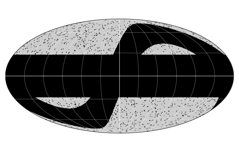
Figure 2: Plot of the sky mask used in our analysis applicable for a space-based weak lensing experiment. Here we see the main galactic-cut as the thick horizontal band, the ecliptic-cut as the slightly thinner sinusoidal band, and our star mask consisting of random circular cut-outs that were generated through the prescription of Section 3.2.1. The galactic- and ecliptic- cuts dominate the large-scale behaviour of the mask, whereas the star mask introduces strong small-scale effects.

3.2.1 Star mask generation

We investigated the statistics of our estimators at a map resolution of $N_{\mathrm{side}}=256$. This corresponds to a pixel angular scale of $14\arcmin$. The prescription described in Martinet et al. (2021) can be followed to generate a realistic Euclid-like star mask. This involves modelling stars as disks that are distributed randomly on the sky and that have a radii drawn from a random uniform distribution taking values between $0.29\arcmin$ and $8.79\arcmin$. Stars can be placed on a map until the desired sky area covered by stars is reached. However, we note that this distribution of radii of stars is smaller than the pixel scale for our map resolution, and so a star mask generated using such values as presented in Martinet et al. (2021) would give rise to under-sampling in the star mask produced, as all stars would be single pixels, which was found to induce errors in the Pseudo-$C_{\ell}$ estimator.

Since we are not after an exact realistic distribution of stars in our analysis, we can instead base our star mask on the distribution of ‘blinding stars’, or avoidance areas, that are expected to be encountered for a space-based observatory (Scaramella et al., 2022). These avoidance areas are expected to have an average area of $0.785\,\mathrm{deg}^{2}$ and total an area of $635\,\mathrm{deg}^{2}$ over the expected survey area. Assuming that these avoidance areas can be modelled as disks, this corresponds to an average radii of $30\arcmin$, and so is large enough to cover multiple pixels in our limited resolution maps. This approximate treatment should capture the main features brought to the analysis by a more realistic star mask.

We used an edited version of the GenStarMask utility as provided with the Flask code (Xavier et al., 2016) to generate our star mask using the avoidance area specification. Our edits were made to draw the radii from a uniform distribution rather than a log-normal. To add some scatter to our avoidance area mask, we generated the disks with radii between $25\arcmin$ and $35\arcmin$. To match the desired total avoidance area, avoidance areas were added until they covered $5\,\%$ of the full-sky.

3.2.2 Power spectrum of mask

Figure 3: Power spectrum of the sky masks used in our analysis. Note that for the ‘main cuts without stars’ curve we plot the even $\ell$-modes only due to the very small values that odd $\ell$-modes take, arising from the parity of the mask.

Since the exact form of Pseudo-$C_{\ell}$ mixing matrix is highly sensitive to the power spectrum of the mask used, through Equation 32, we computed the spherical harmonic transform of our generated mask. This is shown in Figure 3.

We plot the power spectrum for our main galactic- and ecliptic- cuts only, the two cuts with added star mask, and star mask only. For the case without stars added, we plot the $C_{\ell}$ values for even $\ell$-modes only. This is due to the very small values for odd-$\ell$ modes arising from the parity of the mask. Here, we see that the power spectrum for our main mask with stars added has two distinct regions: dominated by the two main cuts for $\ell\lesssim 10^{2}$, and dominated by the star mask above this threshold.

We can understand the primary behaviour of the mask’s power spectrum through computing the analytic power spectrum for a simple mask that is comprised of a single horizontal cut ranging from $\theta=A$ to $\theta=B$. Doing so, we find that the $C_{\ell}$ values are given by

$$C_{\ell}=\frac{\pi}{\left(2\ell+1\right)^{2}}[P_{\ell+1}\left(\cos A\right)-P_{\ell-1}\left(\cos A\right)+\\ -P_{\ell+1}\left(\cos B\right)+P_{\ell-1}\left(\cos B\right)]^{2}.$$ (41)

Enforcing that the mask is symmetric around $\theta=\pi/2$, and using the parity of the Legendre polynomials, we find that the analytic prediction for the odd $\ell$-modes are zero. The addition of a second cut of equal width, for example the ecliptic-cut, keeps the reflective symmetry. While we use a slightly thinner ecliptic-cut, we still keep this approximate symmetry. Propagating these suppressed odd-$\ell$ modes into the mixing matrix through Equation 32 explains the result for why we see strong coupling in the covariance matrices between $C_{\ell}$ values that have even-$\ell$ offsets, and little coupling between odd differences.

We also see that the amplitude of the power spectrum coefficients for the mask without stars generally decreases at larger multipole values, where the $C_{\ell}$ values roughly scale as $\ell^{2}C_{\ell}\propto 1/\ell$. This arises from the large-$\ell$ behaviour of the Legendre polynomials, where they scale as $P_{\ell}\propto 1/\sqrt{\ell}$ (Szegö, 1975).

The behaviour of the power spectrum of the star mask can also be broadly split into two distinct regions. The first is for multipoles $\ell\lesssim 200$ where the $C_{\ell}$ values are constant, which is a result of the random scatter of the stars on the sphere resulting in a noise-like signal. The second is for multipoles larger than $\ell\gtrsim 200$ where the $C_{\ell}$ values start to oscillate in a sinc-like behaviour, which is where the features of the individual circular disks dominate.

3.3 Pseudo-$C_{\ell}$ implementation

An essential part of our work is the accurate computation of the $C_{\ell}$ covariance matrices both for our new QML implementation and its comparison to results obtained using the Pseudo-$C_{\ell}$ method. Here, we used the NaMaster code to produce all estimates for the Pseudo-$C_{\ell}$ method (Alonso et al., 2019).

In general, the computation of the exact Gaussian covariance is a difficult problem that has been discussed extensively in previous literature. In our work, we employed the narrow kernel approximation as presented in García-García et al. (2019) to compute this Gaussian approximation. However, it should be noted that the narrow kernel approximation overestimates the variances for the lowest $\ell$ multipoles. Since it is these exact multipoles that we are most interested in, we instead opt to estimate the covariance from an ensemble of $5\,000$ maps when investigating the raw variances. However, as the estimation of the off-diagonal elements of the covariance matrix are highly sensitive to the number of realisations in the ensemble, when we investigate parameter constraints that are derived from the $C_{\ell}$ covariance matrix, we use the ‘analytic’ result as returned from the narrow kernel approximation. In the limit of using large numbers of realisations in the ensemble, at the cost of extensive run-time, García-García et al. (2019) demonstrated that these two estimation techniques are consistent.

4 Results

4.1 Benchmark against existing estimators

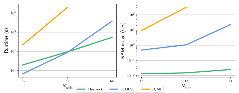
Figure 4: Comparison of RAM usage and run-time for different implementations of the QML estimator. We show that our new method has significantly reduced RAM usage compared to existing estimators, which is why we can extend our method to increased map resolutions that the other methods cannot process. Results were obtained using an average over ten maps for our method, and averaged over three runs for each method at each resolution. Computations were performed using 32 cores of an Intel Cascade Lake processor.

In this section, we present the results of a comparative study between our new QML implementation and the Pseudo-$C_{\ell}$ method. First, we wish to investigate how using the novel techniques employed by our new estimator impacts the ability to recover the power spectrum when compared to existing QML implementations. We compare with two leading public implementations of the QML estimator:

• xQML as presented in Vanneste et al. (2018). This is a straightforward implementation of the QML method as presented in Tegmark (1997) and Tegmark & de Oliveira-Costa (2001) that has been generalised to cross-correlations between maps. It is written primarily in Python with small parts written in C.

• ECLIPSE as presented in Bilbao-Ahedo et al. (2021). This is a more numerically efficient implementation of the QML estimator compared to the original prescription and thus exhibits somewhat better performance scaling with resolution over the naive method. It is written in Fortran.

We wish to compare the performance of our new code, written in C++, with these existing methods. In Figure 4, we present a comparison for the total run-time and RAM usage for the two codes described above and our new method described in this work for a range of map resolutions pushing to the highest $N_{\mathrm{side}}$ possible with these codes and the computational resources available to us. Here, we see that while our new code is competitive in total run-time when compared to ECLIPSE, we see many orders of magnitude improvement in the total RAM usage for our method over the other two methods. This is because we never have to explicitly store, invert, and compute the product of any of the massive $N_{\mathrm{pix}}\times N_{\mathrm{pix}}$ matrices that the other two methods employ. Since we are only interested in computing the action of the covariance matrix on a trial pixel-space vector, we keep all of our working-quantities as $\mathcal{O}(N_{\mathrm{pix}})$ which clearly have much better RAM scaling with resolution over the pixel-space matrices. It is this vastly reduced RAM usage requirement that allows us to push our method to resolutions that are simply not possible on standard high performance clusters using the two previously discussed methods. It is important to note that our new implementation is now only run-time limited, and thus can be pushed to even higher resolutions than have been considered in this work if more extensive computing resources are available. The time-limiting steps to our implementation is the transformations of the trial vector between pixel- and harmonic-space through the use of the HealPix functions alm2map & map2alm. Since both of these functions are implemented using OpenMP parallelism, faster run-times can be achieved through simply running our code on higher core count processors.

Our code is publicly available and can be downloaded from https://github.com/AlexMaraio/WeakLensingQML github.

4.2 Accuracy of numerical Fisher matrix

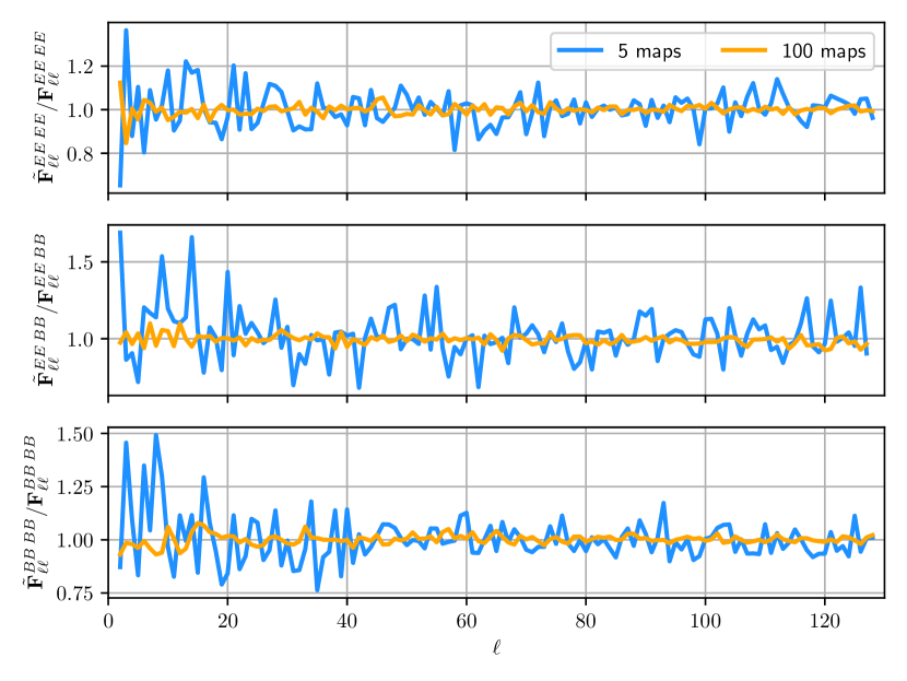
Figure 5: Ratio of our numerical Fisher matrix with respect to the analytic result for a map resolution of $N_{\mathrm{side}}=64$. Here, we plot the diagonal of the $EE$-$EE$, $EE$-$BB$, and $BB$-$BB$ components. All three components show good consistency with unity regardless of the number of maps averaged over when computing the Fisher matrix through Equation 28, with the amplitude of the scatter decreasing with increasing number of maps.

As explained in Section 2.3, we use finite-differences to compute the approximate form of the Fisher matrix from a set of $s_{\ell}$ values estimated using conjugate-gradient techniques. To validate the accuracy of these methods we compared our estimates of the Fisher matrix with the ‘analytic’ result as computed using the formalism presented in Bilbao-Ahedo et al. (2021). While this is still a ‘brute-force’ QML implementation, where the covariance matrix still needs to be computed and stored in full, their method allows many quantities to be expressed in terms of the spherical harmonic transform matrix Y and thus reduce the computational demands of the estimator. This comparison was performed at a map resolution of $N_{\mathrm{side}}=64$, which was the maximum resolution possible for the computation of the analytic result. Note that at this resolution, the typical pixel scale is larger than the angular size of our cut-outs generated for our star mask, and so this comparison was computed for the case without the star mask added to the main cuts. The result of this comparison is presented in Figure 5, where we plot the ratio of the diagonal of the $EE$-$EE$, $EE$-$BB$, and $BB$-$BB$ components of the Fisher matrix. We plot the cases for where we average over five and one hundred maps when injecting power into the generated maps when estimating the Fisher matrix (see Equation 28). Figure 15 shows this ratio extended to several of the off-diagonal strips, specifically for the cases with $\Delta\ell=2,8,32$. Both figures show that while the amplitude of the random scatter in the ratio decreases significantly when averaging over more maps, both cases are simply random scatter around unity - and thus our numerically obtained Fisher matrix is a true representation of the actual Fisher matrix. Propagating the two different numerical and analytical $C_{\ell}$-Fisher matrices to parameter constraints using Fisher forecasts shows negligible differences in parameter contours which again highlights our trust in our new method to estimate the $C_{\ell}$-Fisher matrix at any resolution. Hence, we are free to use our validated method to reliably increase the resolution of our implementation beyond what is possible with current implementations. In our analysis, we averaged over twenty five random realisations which provided a good compromise between run-time and numerical accuracy.

4.3 Comparing $\bm{C_{\ell}}$ variances of QML to Pseudo-$C_{\ell}$

With our new implementation, we can extend the analysis of the properties of the QML estimator to map resolutions of $N_{\mathrm{side}}=256$, which allows us to accurately recover the power spectrum up to a maximum multipole of $\ell_{\mathrm{max}}=512$. At this resolution, the storage of the full pixel covariance matrix alone would require approximately $5\,\mathrm{TB}$ of RAM, which is clearly an unfeasible requirement for any current computer and thus any analysis at this resolution is not achievable using current QML implementations.

We generate maps of the weak lensing shear through producing Gaussian realisations with the power spectrum described in Section 3.1 (see Figure 1). We then add shape noise to these maps according to Equation 39. We generate twenty five such maps for each power spectrum multipole that we are injecting power into ($EE$ and $BB$, from $\ell=2$ to $\ell=767$) and compute the QML power spectrum ($EE$ and $BB$) from each. We estimate the QML covariance matrix using the fact that for Gaussian maps the inverse Fisher matrix is the covariance matrix. The methods described in Section 2.3 were used to estimate the Fisher matrix, where we average over twenty five maps per multipole when evaluating Equation 28. The Pseudo-$C_{\ell}$ covariance matrix was computed using the methods described in Section 3.3, and was constructed from an ensemble of $5\,000$ maps. We do not bin in $\ell$ either of our QML or Pseudo-$C_{\ell}$ estimators, noting that our mask is small enough that the Pseudo-$C_{\ell}$ mixing matrix is invertible without binning as we are able to reconstruct all modes that we have generated. We note that our results were robust to different binning strategies that were applied though not used in our final results.

In Figure 6 we plot the ratio of the standard deviations associated with the Pseudo-$C_{\ell}$ estimator with respect to our QML implementation for the diagonal values associated with the $EE$-$EE$ and $BB$-$BB$ block of the covariance matrix. Here, we see that the Pseudo-$C_{\ell}$ estimator is sub-optimal to the level of $\sim\!\!20\%$ for $\ell\lesssim 50$ for the $EE$ spectra. This corresponds to an equivalent increase in the survey area of around $40\%$ on these scales, which is a massive increase in equivalent area considering that forthcoming Stage-IV surveys are expected to maximise the possible sky area that is observable for ground- or space-based cosmic shear surveys (Scaramella et al., 2022). Hence, getting this additional area ‘for free’ by analysing the data through QML methods demonstrates the advantages of using such methods and such investigations into their behaviour for cosmic shear analyses. For the $BB$ spectra, we find that the Pseudo-$C_{\ell}$ estimator produces errors that are many times that of the optimal QML estimator, peaking at over three times the standard deviation for the Pseudo-$C_{\ell}$ estimator with respect to our QML method. This ratio remains significantly above unity for multipoles that are well above one hundred, which shows that there is a huge advantage to be gained in $B$-mode precision when using QML methods over the Pseudo-$C_{\ell}$ estimator. We find that the ratio for both sets of spectra decays to unity (with some random scatter) for larger $\ell$ values. This matches previous QML studies, which have principally been conducted in the context of the CMB and ground-based galaxy clustering surveys, which found that the Pseudo-$C_{\ell}$ estimator is close to optimal on small scales and for homogenous noise, and we find similar results here in the weak lensing context (Efstathiou, 2004; Leistedt et al., 2013).

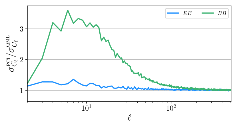
Figure 6: Ratio of standard deviation of the $C_{\ell}$ values (top curve $C_{\ell}^{BB}$, bottom curve $C_{\ell}^{EE}$) obtained using the deconvolved Pseudo-$C_{\ell}$ method using NaMaster to those obtained using our new QML implementation. We see that the QML estimator provides the largest improvements over the Pseudo-$C_{\ell}$ method on the largest angular scales, with a very significant improvement for the $B$-modes.

Figure 6 also shows that the statistical precision of the $B$-mode power spectrum is significantly higher for the QML method compared with Pseudo-$C_{\ell}$ method. This is relevant because cosmic shear theory predicts zero $C_{\ell}^{BB}$ modes and so any detection of a non-zero $C_{\ell}^{BB}$ signal would prompt a thorough investigation of the data (Kilbinger, 2015). Potential sources of $B$-mode power include residual point-spread function uncertainties, telescope detector defects, and intrinsic alignments, all of which should be investigated if non-zero $B$-mode power was found to be statistically significant. The Pseudo-$C_{\ell}$ estimator is very sub-optimal on large scales, and so this loss of sensitivity to the $B$-modes can arise from contamination leakage from the $E$-modes into the $B$-modes due to the nature of the cut-sky. Since the QML estimator is derived from the likelihood for the maps, which depends on the input fiducial power spectrum which contains zero $B$-mode power, any $B$-mode power present in the masked maps must arises from leakage from the $E$-modes, and thus the estimator can weight the data optimality through the covariance matrix to minimise the variance from the $E$-modes contributing to the $B$-modes. For the Pseudo-$C_{\ell}$ estimator, this leakage can be mitigated through the map-level procedure of $B$-mode purification (Lewis et al., 2002; Smith, 2006; Grain et al., 2009) and has been shown to decrease dramatically the associated $B$-mode errors, particularly at low $\ell$ multipoles (Alonso et al., 2019). However, a requirement for purification to work is that the mask must be differentiable along its edges. This can be achieved through the apodisation of the mask which convolves the mask with some smoothing window function that ensures differentiability. This has most commonly been applied to cosmic microwave background experiments where their masks are generally formed of a single much simpler cut applied to the sky (Akrami et al., 2020). This allows apodisation to work effectively on the mask without significant reduction to $f_{\mathrm{sky}}$. However as previously discussed, a weak lensing experiment also needs to mask out small regions corresponding to bright stars or other objects that need removing from the data. These small regions cause significant issues with the apodisation process as the convolution with the smoothing function serves to dramatically increase their apparent area - producing a significant reduction in $f_{\mathrm{sky}}$. We investigate the effects of apodising our mask in Appendix B. We find that while apodisation strongly reduces widely separated mode coupling arising from the suppression in small-scale power of the mask (as now the shape edges from our star-like disks are smoothed out), this could not offset the significant reduction in sky area (from $f_{\mathrm{sky}}=33\,\%$ to $f_{\mathrm{sky}}=22\,\%$) that apodisation brought about. This resulted in apodisation providing looser parameter constraints than for the case without apodisation. A key advantage of the QML estimator is the natural $E$/$B$-mode separation without a loss in sky area (Bunn & Wandelt, 2017).

4.3.1 Varying noise levels

Thus far, we have assumed a noise level corresponding to an experiment that has observed thirty galaxies equally divided into ten redshift bins, giving $\bar{n}=3\,\mathrm{gals/arcmin}^{2}$. Here, we wish to investigate the statistics of our estimators for the case where the observed galaxies are combined into a single redshift bin, giving a much lower noise level of $\bar{n}=30\,\mathrm{gals/arcmin}^{2}$. Performing this comparison produced results as shown in Figure 7. Here, we see that while there is negligible differences in the relative statistics between the $E$-modes, there was a large increase in ratio between our two estimators for the $B$-modes. We can investigate this large difference in the $B$-mode ratios by plotting the raw errors of the $B$-mode spectra for our two estimators for the two noise cases, which is shown in Figure 8.

Here, we see that for low multipoles there is a large difference in the errors for the QML estimator between the two noise levels whereas the errors for the Pseudo-$C_{\ell}$ estimator remains relatively unchanged. At this decreased noise level, the noise is subdominant to the cosmic variance from the $E$-modes on large-scales. Hence, the QML estimator can vastly outperform the Pseudo-$C_{\ell}$ method on these large-scales because the QML likelihood can efficiently minimise the cosmic variance from the $E$-modes leaking into the $B$-modes through the cut-sky. The increased noise level corresponds to a genuine increase in $B$-mode power, which the QML estimator cannot suppress as efficiently as the $E$-mode cosmic variance leakage, and so we see an associated decrease in the ratio between its errors and that of the Pseudo-$C_{\ell}$ estimator.

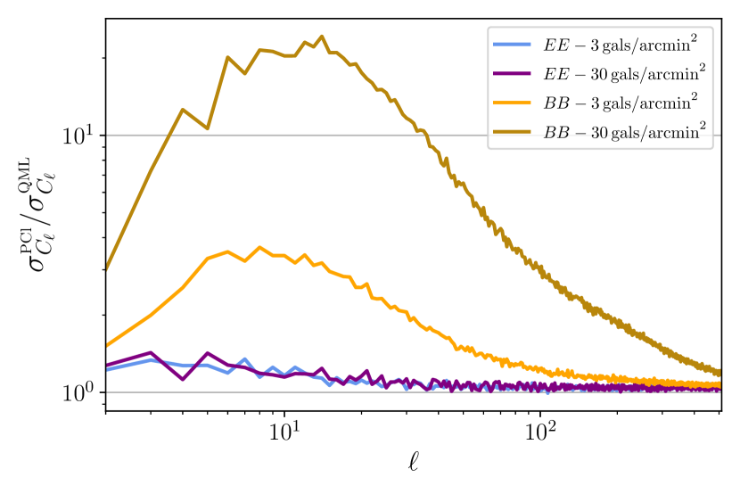
Figure 7: Ratio of the errors on the power spectrum for the Pseudo-$C_{\ell}$ estimator with respect to the QML estimator for the case of two different noise levels of $\bar{n}=3\,\textrm{gals / arcmin}^{2}$ and $\bar{n}=30\,\textrm{gals / arcmin}^{2}$. Here, we see the decreased noise level for the curves for the case of $\bar{n}=3\,\textrm{gals / arcmin}^{2}$ has negligible effect on the errors associated with the $EE$-spectra, whereas there is a large increase in the ratio for the $BB$-spectra.

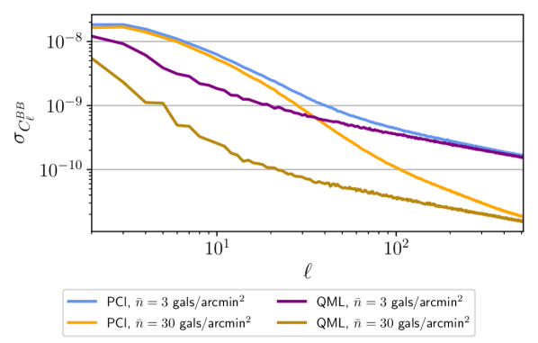
Figure 8: Errors on the $BB$-spectra for the two different noise levels considered. Here, we see that the errors for the Pseudo-$C_{\ell}$ estimator remain relatively unchanged for the lowest multipoles, whereas the errors for the QML estimator decrease dramatically when the amplitude of the noise is reduced.

4.4 Cosmological parameter inference

A Fisher matrix forecast was used to propagate our estimated $C_{\ell}$ covariance matrices into parameter constraints. For an arbitrary set of cosmological parameters $\vartheta_{\alpha}$ and $\vartheta_{\beta}$, the corresponding Fisher matrix element is given by (Tegmark et al., 1997)

$$\mathcal{F}_{\alpha\beta}=\sum_{\ell,\,\ell^{\prime}}\frac{\partial C_{\ell}}{\partial\vartheta_{\alpha}}\,\textbf{{C}}^{-1}_{\ell\ell^{\prime}}\,\frac{\partial C_{\ell^{\prime}}}{\partial\vartheta_{\beta}},$$ (42)

where C is the $C_{\ell}$ covariance matrix. In our analysis, we focused on the two parameters that cosmic shear places the tightest constraints on: the clustering amplitude $S_{8}$ and the total matter density $\Omega_{\mathrm{m}}$. Figure 9 shows a comparison of the derived constraints for these two parameters between our two estimators. Here, we see the effect of the slightly increased errors associated with the Pseudo-$C_{\ell}$ estimator have propagated into slightly increased contours for these two parameters when compared to the QML estimator’s contours. This result could have been anticipated from Figure 6, since most of the information on these parameters originates from small scales where the ratio of the errors approaches unity. In contrast, parameters affecting large angular scales, such as local primordial non-Gaussianity, are expected to benefit substantially from an optimal method.

Figure 9: Parameter constrains on $S_{8}$ and $\Omega_{\mathrm{m}}$ obtained from a Fisher matrix analysis up to a maximum multipole of $\ell_{\mathrm{max}}=512$ for our two estimators. Here, we see that the increased errors associated with the Pseudo-$C_{\ell}$ method propagate through to slightly broadened parameter contours.

The figure of merit, which quantifies how well constrained parameters are, is related to the Fisher matrix through (Blanchard et al., 2020)

$$\mathrm{FoM}_{S_{8}\Omega_{\mathrm{m}}}=\sqrt{\mathrm{det}\left(\mathcal{F}\right)}.$$ (43)

A plot of the figure of merit for the combination of $\Omega_{\mathrm{m}}$ and $S_{8}$ as a function of maximum multipole is shown in Figure 10. Here, we see that the sub-optimality of the Pseudo-$C_{\ell}$ method is most apparent when we are limited to low multipoles. As the maximum multipole increases we see that the figures of merits converge, however showing that the QML method consistently out performs the Pseudo-$C_{\ell}$ method.

The application of Fisher forecasting to predict parameter constraints from the covariance matrix is done under the assumption that the $C_{\ell}$ values recovered from the estimators can be described by a Gaussian likelihood. While it has been shown that for the full sky case, an analytic calculation of the likelihood of the power spectra can be computed (Hall & Taylor, 2022), which can be accurately modelled as a Gaussian on small scales, the exact likelihood of the recovered power spectrum using either the QML or Pseudo-$C_{\ell}$ estimators is still unknown. Previous works have simply used the Gaussian approximation citing the central limit theorem (Seljak et al., 2017). Since QML estimators produce estimates for the full sky power spectrum, we expect this to follow a Gaussian distribution more closely than the cut-sky estimates produced from Pseudo-$C_{\ell}$ methods and so this approximation is expected to hold better for QML over Pseudo-$C_{\ell}$ methods.

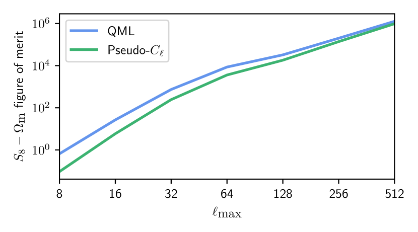
Figure 10: Values for the figure of merit for the combination of $S_{8}$ and $\Omega_{\mathrm{m}}$ as a function of the maximum $\ell$ multipole used in the analysis. We see that as the maximum multipole increases, the relative sub-optimality of the Pseudo-$C_{\ell}$ estimator decreases and results from the two estimators converge.

4.4.1 Inclusion of stars

Our results presented thus far have been all for the case where we have applied a star mask to a large-scale mask featuring ecliptic and galactic cuts, as shown in Figure 2. Here, we wish to investigate the detailed effects on the covariances of our estimators when we apply the star mask to our main two cuts. All results here are presented for the case without any mask apodisation applied.

The ratio of the Pseudo-$C_{\ell}$ covariance matrix for the cases with and without stars is presented in Figure 11. Here, we see that the primary effect of the addition of stars into the mask is to increase the correlation between widely separated $\ell$-modes, while leaving the values close to the diagonal in the covariance matrix relatively unchanged.

This new covariance matrix can then be propagated into parameter contours to see if these increased long-range correlations (which fiducially have very small values) have any meaningful effect on cosmological parameter constraints. This is shown in Figure 12. Here, we see that there are negligible differences on the parameter contours between the two cases for our QML estimator, however there is a slight broadening in the contours for the Pseudo-$C_{\ell}$ estimator which is consistent with the loss of sky area to the star mask. This shows that the Pseudo-$C_{\ell}$ estimator is more sensitive to the addition of a star mask than the QML estimator, further highlighting the benefits of the QML method.

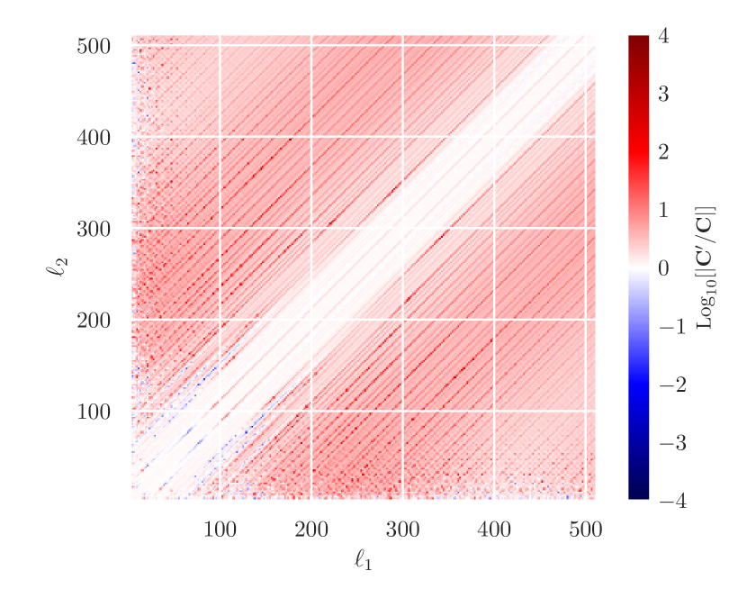
Figure 11: Ratio of the analytic Pseudo-$C_{\ell}$ covariance matrix for the $C_{\ell}^{EE}$ power spectrum for the cases with ($\textbf{{C}}^{\prime}$) and without stars (C) applied to the main mask. Note that we only plot the covariance matrix for even-$\ell$ values only (due to the very small values for the odd-$\ell$ case and so their ratios are dominated by numerical noise).

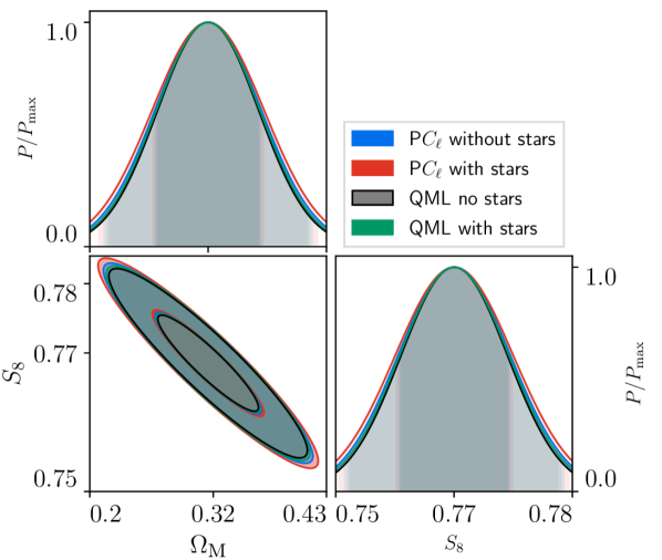
Figure 12: Fisher parameter constraints comparison between QML and Pseudo-$C_{\ell}$, where both estimators have a maximum multipole of $\ell_{\mathrm{max}}=512$, for the cases with and without the star mask applied to both estimators. Here we see that the Pseudo-$C_{\ell}$ estimator is more sensitive to the inclusion of the star mask through the relative increase in parameter contours when compared to the QML contours.

4.5 Non-Gaussian maps

Throughout our paper, we have been applying our estimator to Gaussian realisations of the cosmic shear field. However, as it has been shown that the convergence field $\kappa$ is more accurately described by a log-normal distribution (Taruya et al., 2002; Hilbert et al., 2011), an investigation of how our estimators perform when applied to these non-Gaussian maps was undertaken. This is because as the QML estimator assumes that the underlying power spectrum coefficients follow a Gaussian distribution, any non-Gaussianities present in the shear field could induce non-optimality into the recovered power spectra which would increase errors.

The Flask software package was used to generate log-normal maps (Xavier et al., 2016). The ‘shift parameter’ that corresponds to the minimum value of the convergence field required by Flask was set to 0.01214, following Hall & Taylor (2022). The log-normal maps were generated at a resolution of $N_{\mathrm{side}}=1024$ and then downgraded to a resolution of $N_{\mathrm{side}}=256$ as required to be processed through our estimators. A histogram showing the distribution of $\kappa$ values for a Gaussian and log-normal realisation is shown in Figure 13. This log-normal convergence field is then propagated to a slightly modified shear field, which we can apply the estimators to.

Figure 13: Histogram showing the field values of a Gaussian and log-normal realisation of the convergence field $\kappa$ for the same underlying power spectrum

Figure 14: Ratio of the power spectrum errors for the Pseudo-$C_{\ell}$ method with respect to the QML estimator applied to both Gaussian and log-normal realisations. Here, we see that the results are indistinguishable between the two distributions.

Since the covariance of the QML estimator is no longer given by the inverse Fisher matrix, we have to obtain estimates for the QML errors from an ensemble of numerical realisations. The results of applying the QML and Pseudo-$C_{\ell}$ estimators to an ensemble of $2\,500$ Gaussian and log-normal realisations is shown in Figure 14. Here, we see that the ratio of the power spectrum errors for the two distributions are virtually identical which demonstrates that the relative behaviour of our estimators remains unchanged even when applied to maps that the underlying likelihood does not fully describe. Since the largest differences between the estimators for our setup occur on the largest scales which is where the effects of the non-Gaussianity is weak, this is not surprising.

5 Conclusions

We have presented a new implementation of the optimal quadratic maximum likelihood estimator that is the most efficient publicly available code of its type. Using our new estimator, we have compared the statistical properties of the expected power spectrum for forthcoming Stage-IV weak lensing surveys, using realistic survey conditions, between our QML implementation and an existing Pseudo-$C_{\ell}$ code. We found that the sub-optimality of the Pseudo-$C_{\ell}$ estimator resulted in marginally increased statistical errors for the $E$-mode power spectra propagating to increased parameter contours when using Fisher forecasting. In addition, we found a significant increase in the precision for the $B$-mode power spectra when applying our QML estimator over the Pseudo-$C_{\ell}$ method, which raises the hopes of being able to further constrain new $B$-mode physics using forthcoming surveys. Our results show that the application of QML methods to cosmic shear data provides a useful cross-check to existing methods, and could have many interesting applications for the constraints of new $B$-mode physics.

Our new estimator could be extended in numerous ways, for example the QML method can be easily applied to spin-0 fields such as photometric galaxy clustering. Since our estimator yield the best improvements on the largest physical scales, scales at which primordial non-Gaussianity has the largest effects on the observed signal, the use of our new estimator could enable tighter constraints on primordial non-Gaussianity. In addition, photometric galaxy clustering data can be combined with cosmic shear to form a combined $3\times 2$-point investigation which our estimator could be applied to. We leave these applications of our estimator to future work. We also note that our estimator could also be applied to thermal Sunyaev-Zeldovich data, which is a powerful probe of cosmology at relatively low multipoles ($\ell\lesssim 10^{3}$) (Horowitz & Seljak, 2017; Bolliet et al., 2018). This overlaps with the multipole region where QML provides the best improvements over the Pseudo-$C_{\ell}$ estimator, and so could provide sufficiently tighter constraints when applied to these data-sets.

Since QML methods deal with data at the pixel-level, they are well suited for dealing with contaminants and effects that can only be described accurately in terms of pixels in the maps. One such problem is the effect of spatially varying noise over survey area, which could arise from different seeing conditions encountered as a telescope surveys the sky or the properties of the detector evolving as data is taken. These effects can easily be incorporated into the QML estimator through an appropriate modification of the noise matrix N, whereas the Pseudo-$C_{\ell}$ method utilises Fourier transforms and these pixel-level effects get diffused over a wide $\ell$ range and thus become harder to model. This could further reduce the optimality of the Pseudo-$C_{\ell}$ estimator. We leave a dedicated investigation of how such effects affect the two estimators to future work.

To conclude, we have shown that the Pseudo-$C_{\ell}$ estimator is close to optimal on small scales for a simplified Euclid-like weak lensing survey. Despite this, the QML estimator is better suited for a variety of applications, including $E$/$B$-mode separation, complex noise patterns, and complicated survey geometries. With systematics expected to dominate the error budget of upcoming surveys it is increasingly important to demonstrate the consistency of results derived from different analysis pipelines - the fast, publicly available implementation of the QML estimator that we have presented in this work represents a significant step forward in this regard.

Data availability

All data presented in this work has been generated by the authors. The code to do so can be found on our GitHub repository located at https://github.com/AlexMaraio/WeakLensingQML github.

Appendix A Ratio of numeric to analytic Fisher

Figure 15 shows the ratio of our numerically computed $C_{\ell}$ Fisher matrix to that computed using analytic methods for a number of different off-set values from the diagonal. Here, we see that all curves simply exhibit random scatter around unity which shows that our numerical estimates of the Fisher matrix is an unbiased estimate of the true values. The residual noise in the Fisher matrix gives rise to negligible differences in parameter confidence contours.

Figure 15: Ratio of our numerically-derived $C_{\ell}$-Fisher matrix to the analytic result for a map resolution of $N_{\mathrm{side}}=64$, presented for the cases where we average over five and one hundred maps. Here, we plot the $EE$-$EE$, $EE$-$BB$, and $BB$-$BB$ components separately, with varying off-sets from the diagonal in the different columns. We see good agreement between our estimator and existing results for all combination of spectra and off-sets, and so deduce that our numerical estimate is consistent with the analytic result.

Appendix B Sensitivity to apodisation

Previously, we have discussed how apodisation of the mask is not required for QML methods whereas there are certain advantages to doing so for the Pseudo-$C_{\ell}$ method. This is because apodisation reduces the effects of sharp edges that may be present in the mask. To investigate the effects of apodisation, we have applied a $2^{\circ}$ apodisation using the $\mathcal{C}^{2}$ scheme as described in Alonso et al. (2019) to our mask, including stars. We note that for this apodisation scale and scheme, the sky area reduces from $f_{\mathrm{sky}}=33\,\%$ to $f_{\mathrm{sky}}=22\,\%$. Figure 16 shows the power spectrum of our mask with and without apodisation applied. Here, we see that the effect of apodisation is to vastly reduce the small-scale power of the mask. The effect of this suppression of small-scale power results in the reduction in long-range correlations in the covariance matrix, as can be shown from Equation 35, and thus the computation and inversion of the mixing matrix should be more accurate when apodisation is applied. The ratio of the analytic Pseudo-$C_{\ell}$ covariance matrix for the $C_{\ell}^{EE}$ spectrum for the cases of with and without apodisation is shown in Figure 17. This shows that for values along and close to the diagonal, the loss of sky area causes significant increases in the variances in the power spectrum. For mode-pairs that are highly separated we see a notable decrease in their covariances, which once again can be seen from Equation 35.

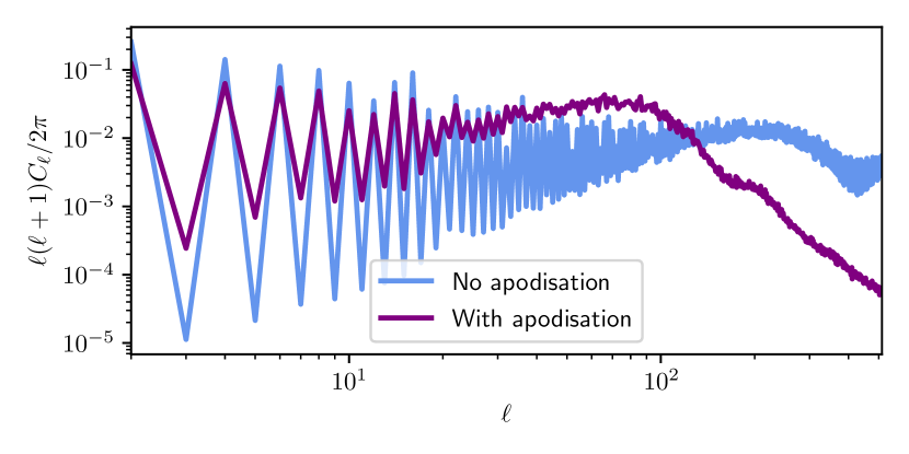
Figure 16: Power spectrum of our mask, with stars included, for cases with and without apodisation applied.

Figure 17: Ratio of the analytic Pseudo-$C_{\ell}$ covariance matrix for the $C_{\ell}^{EE}$ power spectrum for the cases with ($\textbf{{C}}^{\prime}$) and without (C) mask apodisation applied.

Figure 18 shows the ratio of the errors for the Pseudo-$C_{\ell}$ (the square-root of the diagonal of the covariance matrix) with respect to our QML estimator for the case of with and without apodisation. Here, we see that the effect of apodisation is to increase the errors of the Pseudo-$C_{\ell}$ method - which is a direct result in the loss of sky area that apodisation produces.

Figure 18: Ratio of $C_{\ell}$ errors of the Pseudo-Cl method with respect to our QML estimator for the cases with and without apodisation.

The covariance matrix for the case where we have applied apodisation can then be propagated into parameter constraints, which is shown in Figure 19. Here, we see that the direct loss of sky area associated with apodisation results in broadened parameter contours which is not offset by the decrease in long-range correlations that apodisation suppresses in the covariance matrix.

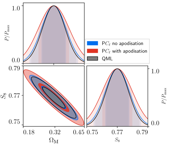
Figure 19: Fisher parameter constraints comparison between QML and Pseudo-$C_{\ell}$ where both estimators have a maximum multipole of $\ell_{\mathrm{max}}=512$ and for the case where apodisation has been applied for the Pseudo-$C_{\ell}$ method. We see a large broadening for the Pseudo-$C_{\ell}$ contour with apodisation applied, which is consistent with the loss of sky area that apodisation results in.

References

- Abate et al. (2012) Abate A., et al., 2012, arXiv e-prints (1211.0310)
- Abdalla et al. (2022) Abdalla E., et al., 2022, JHEAp, 34, 49
- Akrami et al. (2020) Akrami Y., et al., 2020, Astron. Astrophys., 641, A4
- Alonso et al. (2019) Alonso D., Sanchez J., Slosar A., 2019, Mon. Not. Roy. Astron. Soc., 484, 4127
- Asgari et al. (2021) Asgari M., et al., 2021, Astron. Astrophys., 645, A104
- Bartelmann (2010) Bartelmann M., 2010, Class. Quant. Grav., 27, 233001
- Bartelmann & Schneider (2001) Bartelmann M., Schneider P., 2001, Phys. Rept., 340, 291
- Bilbao-Ahedo et al. (2017) Bilbao-Ahedo J. D., Barreiro R. B., Herranz D., Vielva P., Martínez-González E., 2017, JCAP, 02, 022
- Bilbao-Ahedo et al. (2021) Bilbao-Ahedo J. D., Barreiro R. B., Vielva P., Martínez-González E., Herranz D., 2021, JCAP, 07, 034
- Blanchard et al. (2020) Blanchard A., et al., 2020, Astron. Astrophys., 642, A191
- Bolliet et al. (2018) Bolliet B., Comis B., Komatsu E., Macías-Pérez J. F., 2018, Mon. Not. Roy. Astron. Soc., 477, 4957
- Bond et al. (1998) Bond J. R., Jaffe A. H., Knox L., 1998, Phys. Rev. D, 57, 2117
- Brown et al. (2005) Brown M. L., Castro P. G., Taylor A. N., 2005, Mon. Not. Roy. Astron. Soc., 360, 1262
- Bunn & Wandelt (2017) Bunn E. F., Wandelt B., 2017, Phys. Rev. D, 96, 043523
- Chisari et al. (2019) Chisari N. E., et al., 2019, Astrophys. J. Suppl., 242, 2
- Chon et al. (2004) Chon G., Challinor A., Prunet S., Hivon E., Szapudi I., 2004, Mon. Not. Roy. Astron. Soc., 350, 914
- Doux et al. (2022) Doux C., et al., 2022, arXiv e-prints (2203.07128)
- Efstathiou (2004) Efstathiou G., 2004, Mon. Not. Roy. Astron. Soc., 349, 603
- Efstathiou (2006) Efstathiou G., 2006, Mon. Not. Roy. Astron. Soc., 370, 343
- Elsner & Wandelt (2013) Elsner F., Wandelt B. D., 2013, Astron. Astrophys., 549, A111
- Estrada et al. (2022) Estrada N., Granett B. R., Guzzo L., 2022, Mon. Not. Roy. Astron. Soc., 512, 2817
- García-García et al. (2019) García-García C., Alonso D., Bellini E., 2019, JCAP, 11, 043
- Gorski et al. (2005) Gorski K. M., Hivon E., Banday A. J., Wandelt B. D., Hansen F. K., Reinecke M., Bartelman M., 2005, Astrophys. J., 622, 759
- Grain et al. (2009) Grain J., Tristram M., Stompor R., 2009, Phys. Rev. D, 79, 123515
- Hall & Taylor (2022) Hall A., Taylor A., 2022, arXiv e-prints (2202.04095)
- Hamana et al. (2020) Hamana T., et al., 2020, Publ. Astron. Soc. Jap., 72, 16
- Heymans et al. (2021) Heymans C., et al., 2021, Astron. Astrophys., 646, A140
- Hikage et al. (2011) Hikage C., Takada M., Hamana T., Spergel D., 2011, Mon. Not. Roy. Astron. Soc., 412, 65
- Hikage et al. (2019) Hikage C., et al., 2019, Publ. Astron. Soc. Jap., 71, 43
- Hilbert et al. (2011) Hilbert S., Hartlap J., Schneider P., 2011, Astron. Astrophys., 536, A85
- Hivon et al. (2002) Hivon E., Gorski K. M., Netterfield C. B., Crill B. P., Prunet S., Hansen F., 2002, Astrophys. J., 567, 2
- Horowitz & Seljak (2017) Horowitz B., Seljak U., 2017, Mon. Not. Roy. Astron. Soc., 469, 394
- Horowitz et al. (2019) Horowitz B., Seljak U., Aslanyan G., 2019, JCAP, 10, 035
- Hu (2000) Hu W., 2000, Phys. Rev. D, 62, 043007
- Hu & White (2001) Hu W., White M. J., 2001, Astrophys. J., 554, 67
- Kaiser (1992) Kaiser N., 1992, Astrophys. J., 388, 272
- Kilbinger (2015) Kilbinger M., 2015, Rept. Prog. Phys., 78, 086901
- Köhlinger et al. (2016) Köhlinger F., Viola M., Valkenburg W., Joachimi B., Hoekstra H., Kuijken K., 2016, Mon. Not. Roy. Astron. Soc., 456, 1508
- Köhlinger et al. (2017) Köhlinger F., et al., 2017, Mon. Not. Roy. Astron. Soc., 471, 4412
- Laureijs et al. (2011) Laureijs R., et al., 2011, arXiv e-prints (1110.3193)
- Leistedt et al. (2013) Leistedt B., Peiris H. V., Mortlock D. J., Benoit-Lévy A., Pontzen A., 2013, Mon. Not. Roy. Astron. Soc., 435, 1857
- Lewis et al. (2002) Lewis A., Challinor A., Turok N., 2002, Phys. Rev. D, 65, 023505
- Lin et al. (2012) Lin H., et al., 2012, Astrophys. J., 761, 15
- Loureiro et al. (2021) Loureiro A., et al., 2021, arXiv e-prints (2110.06947)
- Martinet et al. (2021) Martinet N., Harnois-Déraps J., Jullo E., Schneider P., 2021, Astron. Astrophys., 646, A62
- McDonald (2019a) McDonald P., 2019a, Phys. Rev. D, 99, 043538
- McDonald (2019b) McDonald P., 2019b, Phys. Rev. D, 100, 043511
- Mortlock et al. (2002) Mortlock D. J., Challinor A. D., Hobson M. P., 2002, Mon. Not. Roy. Astron. Soc., 330, 405
- Nicola et al. (2021) Nicola A., García-García C., Alonso D., Dunkley J., Ferreira P. G., Slosar A., Spergel D. N., 2021, JCAP, 03, 067
- Oh et al. (1999) Oh S. P., Spergel D. N., Hinshaw G., 1999, Astrophys. J., 510, 551
- Pen (2003) Pen U.-L., 2003, Mon. Not. Roy. Astron. Soc., 346, 619
- Philcox (2021) Philcox O. H. E., 2021, Phys. Rev. D, 103, 103504
- Ramanah et al. (2018) Ramanah D. K., Lavaux G., Wandelt B. D., 2018, Mon. Not. Roy. Astron. Soc., 476, 2825
- Scaramella et al. (2022) Scaramella R., et al., 2022, Astron. Astrophys., 662, A112
- Schneider et al. (2002) Schneider P., van Waerbeke L., Kilbinger M., Mellier Y., 2002, Astron. Astrophys., 396, 1
- Schneider et al. (2010) Schneider P., Eifler T., Krause E., 2010, Astron. Astrophys., 520, A116
- Seljak (1998) Seljak U., 1998, Astrophys. J., 506, 64
- Seljak et al. (2017) Seljak U., Aslanyan G., Feng Y., Modi C., 2017, JCAP, 12, 009
- Smith (2006) Smith K. M., 2006, Phys. Rev. D, 74, 083002
- Spergel et al. (2015) Spergel D., et al., 2015, arXiv e-prints (1503.03757)
- Szapudi et al. (2000) Szapudi I., Prunet S., Pogosyan D., Szalay A. S., Bond J. R., 2000, ApJ, 548, L115
- Szegö (1975) Szegö G., 1975, Orthogonal Polynomials. American Math. Soc: Colloquium publ, American Mathematical Society
- Taruya et al. (2002) Taruya A., Takada M., Hamana T., Kayo I., Futamase T., 2002, Astrophys. J., 571, 638
- Tegmark (1997) Tegmark M., 1997, Phys. Rev. D, 55, 5895
- Tegmark & de Oliveira-Costa (2001) Tegmark M., de Oliveira-Costa A., 2001, Phys. Rev. D, 64, 063001
- Tegmark et al. (1997) Tegmark M., Taylor A., Heavens A., 1997, Astrophys. J., 480, 22
- Thomas et al. (2017) Thomas D. B., Whittaker L., Camera S., Brown M. L., 2017, Mon. Not. Roy. Astron. Soc., 470, 3131
- Upham et al. (2021) Upham R. E., et al., 2021, arXiv e-prints (2112.07341)
- Vanneste et al. (2018) Vanneste S., Henrot-Versillé S., Louis T., Tristram M., 2018, Phys. Rev. D, 98, 103526
- Xavier et al. (2016) Xavier H. S., Abdalla F. B., Joachimi B., 2016, Mon. Not. Roy. Astron. Soc., 459, 3693
- van Uitert et al. (2018) van Uitert E., et al., 2018, Mon. Not. Roy. Astron. Soc., 476, 4662