Bayesian Sparse Gaussian Mixture Model in High Dimensions

Abstract

We study the sparse high-dimensional Gaussian mixture model when the number of clusters is allowed to grow with the sample size. A minimax lower bound for parameter estimation is established, and we show that a constrained maximum likelihood estimator achieves the minimax lower bound. However, this optimization-based estimator is computationally intractable because the objective function is highly nonconvex and the feasible set involves discrete structures. To address the computational challenge, we propose a Bayesian approach to estimate high-dimensional Gaussian mixtures whose cluster centers exhibit sparsity using a continuous spike-and-slab prior. Posterior inference can be efficiently computed using an easy-to-implement Gibbs sampler. We further prove that the posterior contraction rate of the proposed Bayesian method is minimax optimal. The mis-clustering rate is obtained as a by-product using tools from matrix perturbation theory. The proposed Bayesian sparse Gaussian mixture model does not require pre-specifying the number of clusters, which can be adaptively estimated via the Gibbs sampler. The validity and usefulness of the proposed method is demonstrated through simulation studies and the analysis of a real-world single-cell RNA sequencing dataset.

Keywords: Clustering, High dimensions, Markov chain Monte Carlo, Minimax estimation, Posterior contraction.

1 Introduction

Clustering is a powerful tool for detecting structures in heterogeneous data and identifying homogeneous subgroups with a wide range of applications, such as genomics (Gu and Liu,, 2008), pattern recognition (Diday et al.,, 1981), compute vision (Georghiades et al.,, 2001), and topic modeling (Blei et al.,, 2003). In many scientific domains, data are often high-dimensional, i.e., the dimension of observations can be much larger than the sample size. For example, an important task in the analysis of single-cell RNA-sequencing data, where the number of genes (dimension) is usually larger than the number of cells (sample size), is to cluster cells and identify functional cell subpopulations (Cao et al.,, 2019). A principal challenge of extending the low-dimensional clustering techniques to high dimensions is the well-known “curse of dimensionality.” To overcome this issue, dimensionality reduction (Ding et al.,, 2002) or additional structural assumptions (Cai et al.,, 2019) are usually necessary in high dimensional clustering methods.

High dimensional clustering and mixture models have attracted attention recently from the frequentist perspective. When the dimension $p$ has at most the same order as the sample size $n$, Doss et al., (2021) studied the optimal rate of estimation in a finite Gaussian location mixture model without a separation condition. Löffler et al., (2021) showed that spectral clustering is minimax optimal in the Gaussian mixture model with isotropic covariance matrix when $p=o(n\Delta)$, where $\Delta$ is the minimal distance among cluster centers. When $p\gg n$, Azizyan et al., (2013) considered a simple case in which there are only two clusters with equal mixing weights and same isotropic covariance matrices. Jin and Wang, (2016) and Jin et al., (2017) proposed influential features principal cluster analysis based on feature selection and principal component analysis. A phase transition phenomenon in high dimensional clustering problem was also investigated in Jin and Wang, (2016) and Jin et al., (2017) across different sparsity and signal levels. Cai et al., (2019) proposed a modified expectation-maximization algorithm based on sparse discriminant vectors to obtain the minimax optimal convergence rate of the excess mis-clustering error. In terms of density estimation, Ashtiani et al., (2020) obtained a near-optimal convergence rate for high dimensional location-scale mixtures with respect to the total variation distance.

Despite these theoretical and computational developments in high dimensional clustering, most frequentist approaches dealing with finite mixtures assume that the number of clusters $K$ is either known or needs to be estimated consistently using techniques such as cross-validation (Smyth,, 2000) and the gap statistics (Tibshirani et al.,, 2001). In contrast, Bayesian methods treat $K$ as an unknown parameter and put a prior on it. For example, Miller and Harrison, (2018) proposed a mixture of finite mixtures model with a computationally efficient Gibbs sampler, and the posterior consistency of $K$ was later studied in Miller, (2018). Ohn and Lin, (2022) established a near optimal rate for estimating finite Gaussian mixtures with respect to the Wasserstein distance when $K$ is unknown and allowed to grow with $n$. In the context of Bayesian model-based clustering for high-dimensional data, Tadesse et al., (2005) suggested to first conduct certain variable selection procedures, and then apply a low-dimensional clustering algorithm with a prior on the number of clusters. Alternatively, Chandra et al., (2022) proposed a Bayesian latent factor mixture model and investigated the behavior of the induced cluster memberships as $p$ goes to infinity whereas $n$ remains fixed. However, a general theoretical framework for Bayesian analysis of high-dimensional clustering is yet to be established.

The Gaussian mixture model we consider lies in the regime of high dimensionality with sparsity structures. There has been a growing interest in Bayesian inference with sparsity-enforcing priors. One commonly-used prior is the spike-and-slab prior (Mitchell and Beauchamp,, 1988), which is a mixture of a point mass at zero and a relatively “flat” absolutely continuous density. The spike-and-slab LASSO prior proposed by Ročková and George, (2018) borrows the similarity between the LASSO and Laplace priors, and combines it with a continuous version of the spike and slab prior. Theoretical properties of the spike-and-slab LASSO prior were well studied in the context of regression models, graphical models, and Gaussian sequence models (see Bai et al.,, 2021 for a review). Another class of sparsity-enforcing priors is global-local shrinkage priors, such as the horseshoe prior (Carvalho et al.,, 2009) and the Dirichlet-Laplace prior (Bhattacharya et al.,, 2015). We refer the readers to Tadesse and Vannucci, (2021) and references therein. However, it is not clear whether these types of prior can be adapted to sparse clustering problems with an unknown number of clusters.

This paper presents the Bayesian analysis of a high-dimensional sparse Gaussian mixture model using a spike-and-slab LASSO prior and establishes the optimality of the proposed estimation procedure. Our main contribution is threefold. First, we fully characterize the minimax rate for parameter estimation in the high-dimensional sparse Gaussian mixture model, and prove that a constrained maximum likelihood estimator achieves minimax optimality. Second, we propose a computationally-tractable Bayesian sparse Gaussian mixture model, and show that its posterior contraction rate is minimax optimal. A posterior contraction rate for the misclustering error is also obtained using tools from matrix perturbation theory (Yu et al., 2014a, ). Third, the proposed Bayesian model not only provides a natural way to characterize uncertainty in clustering, but also estimates the number of clusters adaptively without specifying it a priori. In particular, the number of clusters is not required to be fixed and allowed to grow with the sample size.

The rest of this paper is organized as follows. In Section 2, we introduce the high-dimensional clustering problem and our model, establish the minimax lower bound for parameter estimation, and propose a frequentist constrained maximum likelihood estimator that achieves the minimax lower bound. Section 3 elaborates on the main theoretical results, including the optimal posterior contraction rate and the mis-clustering error. We demonstrate the practical performance of the proposed methodology through simulation studies in Section 4 and a real-world application to clustering single-cell RNA sequencing data in Section 5.

Notations: Let $|S|$ denote the cardinality of $S$ if the set $S$ is finite or the volume (Lebesgue measure) of $S$ if $S$ is a Lebesgue-measurable infinite subset in Euclidean space. Denote $[n]$ as the set of all consecutive integers $\{1,\dots,n\}$. We use $\lesssim$ and $\gtrsim$ to denote the inequality up to a constant. In other words, $a\lesssim(\gtrsim\text{, resp.})$ $b$ if $a\leq(\geq\text{, resp.})$ $Cb$ for some constant $C>0$. We write $a\asymp b$ if $a\lesssim b$ and $b\lesssim a$. We use $\lfloor x\rfloor$ to denote the greatest integer less than or equal to the real number $x$ and $\lceil x\rceil$ to denote the smallest integer greater than or equal to the real number $x$. For a $p$-dimensional vector $\bm{x}\in\mathbb{R}^{p}$, we denote $x_{i}$ as the $i$th coordinate of $\bm{x}$. Also, we denote $\|\bm{x}\|_{1}=\sum_{i=1}^{p}|x_{i}|$ as the $\ell_{1}$-norm, $\|\bm{x}\|_{2}=\sum_{i=1}^{p}|x_{i}|^{2}$ as the $\ell_{2}$-norm, $\|\bm{x}\|_{\infty}=\max_{i\in[p]}|x_{i}|$ as the $\ell_{\infty}$-norm, and $\|\bm{x}\|_{0}=\sum_{i=1}^{p}\mathbbm{1}(x_{i}\neq 0)$. For any matrix $\bm{A}\in\mathbb{R}^{n\times m}$, let $A_{ij}$ denote the $(i,j)$-entry of $\bm{A}$ and let $\bm{A}_{i\cdot}$ and $\bm{A}_{\cdot j}$ be the $i$th row and $j$th column of $\bm{A}$, respectively. We denote $\|\bm{A}\|_{F}=\sqrt{\sum_{i=1}^{n}\sum_{j=1}^{m}|A_{ij}|^{2}}$ to be the Frobenius norm of $\bm{A}$ and $\|\bm{A}\|_{2}$ to be the spectral norm of $\bm{A}$. The prior and posterior probability distributions are denoted as $\Pi$ and the corresponding densities with respect to the underlying $\sigma$-finite measure (whenever it exists) are denoted as $\pi$. We denote $D_{KL}(\mathbb{P}\|\mathbb{Q})$ the Kullback–Leibler divergence between any probability measures $\mathbb{P}$ and $\mathbb{Q}$. The $\epsilon$-packing number of a metric space $\Theta$ with respect to the metric $d$, which is the maximum number of pairwise disjoint balls contained $\Theta$ with radii $\epsilon$, is denoted as $M(\epsilon,\Theta,d)$. In the rest of the paper, we will use an asterisk to represent the ground true values of the parameters that give rise to the data distribution.

2 Model

2.1 Gaussian mixture model and clustering

Let $\bm{Y}=[\bm{Y}_{1},\dots,\bm{Y}_{n}]$ be a $p\times n$ data matrix, where rows represent variables or features, and columns represent observations. We assume that the data exhibits a clustering structure that can be described through a Gaussian mixture model as follows. Let $\bm{\mu}_{1},\dots,\bm{\mu}_{K}\in\mathbb{R}^{p}$ be the cluster centroids of the respective clusters, where $K\geq 1$ is the number of clusters. Let $\bm{z}=(z_{1},\dots,z_{n})^{T}\in[K]^{n}$ be the cluster membership vector for observations, with $z_{i}=k$ indicating that $\bm{Y}_{i}$ belongs to the $k$th cluster associated with the cluster centroid $\bm{\mu}_{k}$. The distribution of $\bm{Y}_{i}$ is given by

$$\bm{Y}_{i}=\bm{\mu}_{z_{i}}+\bm{\epsilon}_{i},$$ (1)

where $\bm{\epsilon}_{i}\sim N_{p}(0,\bm{I}_{p})$ independently for $i\in[n]$. The goal is to estimate the cluster centroids $\bm{\mu}_{1},\ldots,\bm{\mu}_{K}$ as well as to recover the latent cluster membership vector $\bm{z}$.

Remark 1.

We assume that the covariance matrices of the noise $\epsilon_{i}$’s are the homoskedastic identity matrix for ease of theoretical treatment. Our methodology can be easily extended to the heteroskedastic case where the covariance matrices are diagonal with unknown diagonal entries. However, the generalization to more complicated scenarios beyond diagonal covariance matrices is a challenging problem as the number of parameters grows with the dimension and brings extra difficulty for parameter estimation.

Remark 2.

The cluster assignment variables $z_{i}$’s here are treated as unknown but deterministic parameters rather than latent random variables. In some contexts, the Gaussian mixture model (Fraley and Raftery,, 2002) is assumed to have the density of the mixture form, namely, $p(y_{i})=\int\phi(y_{i}\mid{\theta})dF({\theta})$, where $\phi$ is the Gaussian kernel with parameter $\theta$ and $F=\sum_{k=1}^{K}w_{k}\delta_{\bm{\mu}_{k}}$ is a finite discrete mixing measure with $\delta$ being the Dirac measure. In this setup, $z$ becomes a random variable with a categorical distribution given by $P(z_{i}=k)=w_{k}$, $k\in[K]$. Then the joint log-likelihood function of the data $\bm{Y}$ can be written as

$$L_{1}(w_{1},\dots,w_{K},\bm{\mu}_{1},\dots,\bm{\mu}_{K};\bm{Y})=\sum_{i=1}^{n}\log\left(\sum_{k=1}^{K}w_{k}\phi(\bm{Y}_{i}\mid\bm{\mu}_{k},\bm{I}_{p})\right),$$ (2)

where $\phi(\cdot\mid\bm{\mu}_{k},\bm{I}_{p})$ represents the density function of $N_{p}(\bm{\mu}_{k},\bm{I}_{p})$. In our setup with the $z_{i}$’s being unknown parameters, the joint log-likelihood function becomes

$$L_{2}(z,\bm{\mu}_{1},\dots,\bm{\mu}_{K};\bm{Y})=-\frac{np}{2}\log(2\pi)-\frac{1}{2}\sum_{i=1}^{n}\left\|\bm{Y}_{i}-\bm{\mu}_{z_{i}}\right\|_{2}^{2}.$$ (3)

The log-likelihood function (3) can be viewed as the conditional log-likelihood function of (2) given the cluster memberships $z$. Consequently, viewed from the random cluster membership perspective, our framework can be treated as the inference based on the conditional likelihood function given $z$.

This paper considers the asymptotic regime where both $p$ and $n$ go to infinity and $p/n\to\infty$. When $p$ does not exceed $n$, Azizyan et al., (2013) proved that the expected clustering accuracy (which will be defined formally later) depends on the dimension $p$ through the rate $\sqrt{p/n}$ in the two-cluster problem without additional structural assumptions. Under the regime that $p/n\to\infty$ considered in our framework, we posit the following sparse structure on the cluster mean vectors $\bm{\mu}_{1},\ldots,\bm{\mu}_{K}$. Denote $\bm{\mu}=[\bm{\mu}_{1},\ldots,\bm{\mu}_{K}]$ as the matrix concatenated by the mean vectors of all clusters and define the support of $\bm{\mu}$ as $\text{supp}(\bm{\mu})=\{j\in[p]:(\bm{\mu}_{j\cdot})^{T}\neq 0\}$. We say that $\bm{\mu}$ is jointly $s$-sparse if $|\text{supp}(\bm{\mu})|\leq s$. Moreover, we require that not only each $\bm{\mu}_{k}$ has at most $s_{n}$ non-zero coordinates, namely, $\sum_{j=1}^{p}\mathbbm{1}(\mu_{kj}\neq 0)\leq s_{n}$ for all $k\in[K]$, but also that $\bm{\mu}$ is jointly $s_{n}$-sparse. We assume $s_{n}\to\infty$ as $n\to\infty$. In the sequel, we will drop the subscript $n$ from $s_{n}$ and write $s=s_{n}$ for notation simplicity, but the readers should be reminded that $s$ depends on $n$ implicitly.

Denote $\bm{e}_{i}\in\mathbb{R}^{K}$ the unit vector that has value 1 at the $i$th coordinate and $0$ elsewhere. Let $\bm{L}=[\bm{l}_{1},\dots,\bm{l}_{n}]^{T}\in\mathbb{R}^{n\times K}$ where $\bm{l}_{i}=\bm{e}_{z_{i}}$. Then $\bm{L}$ is the matrix whose rows represent cluster memberships of the $n$ observations. It follows immediately that the expected data matrix can be written as $\operatorname{\mathbb{E}}(\bm{Y})=\bm{\mu}\bm{L}^{T}$. Namely, our model can be represented as a signal-plus-noise model matrix $\bm{Y}=\bm{\mu}\bm{L}^{T}+\bm{E}$, where $\bm{E}=[\bm{\epsilon}_{1},\dots,\bm{\epsilon}_{n}]$ is the mean-zero noise matrix whose elements are independent standard normal random variables. As $K$ is typically much smaller than $n$, the above representation of the model is similar to those in Cape et al., (2018) and Agterberg et al., (2022) because the data matrix has a low expected rank. Nevertheless, the sparse Gaussian mixture model differs from Cape et al., (2018) and Agterberg et al., (2022) in that the columns of the expected data matrix have the clustering structure and the rows have the sparsity structure. Following the previous convention of using asterisk to indicate true parameter values, we denote $\bm{\mu}^{*}$ and $\bm{L}^{*}$ the underlying truth of $\bm{\mu}$ and $\bm{L}$ throughout the rest of the paper.

2.2 Minimax lower bound

One of the major theoretical contributions of this paper is to study the estimation error of the mean matrix $(\bm{\mu}^{*})(\bm{L}^{*})^{T}$ in the proposed sparse Gaussian mixture model. As the first step towards the complete theory, we establish the minimax lower bound. Formally, consider the following parameter space

$$\Theta^{*}_{K}=\left\{(\bm{\mu},\bm{L}):\bm{\mu}\in\mathbb{R}^{p\times K},\bm{L}\in\mathcal{L}_{K},|\mathrm{supp}(\bm{\mu})|\leq s,\|\bm{\mu}\bm{L}^{T}\|_{F}^{2}=O(sn)\right\},$$

where $\mathcal{L}_{K}=\{\bm{L}\in\mathbb{R}^{n\times K}:\bm{L}=[\bm{l}_{1},\dots,\bm{l}_{n}]^{T},\bm{l}_{i}\in\{0,1\}^{K},\|\bm{l}_{i}\|_{0}=1\text{ for all }i\in[n]\}$ is the set of all cluster assignment matrices and $\mathrm{supp}(\bm{\mu})$ is the set of indices of the non-zero rows of $\bm{\mu}$.

We next present a collection of assumptions that are necessary in the rest of the theoretical analysis.

Assumption 1.

(Low rank) $K\log n\lesssim\log p$.

Assumption 2.

(Minimum separation) $\Delta=\min_{k_{1}\neq k_{2}}\|\bm{\mu}^{*}_{k_{1}}-\bm{\mu}^{*}_{k_{2}}\|_{2}$ is lower bounded by some constant $c>0$.

Assumption 3.

(High dimensionality) $p/n\to\infty$.

Assumption 1 is a mild low-rank assumption and can be satisfied even with increasing $K$. Assumption 2 requires that the centroids of different clusters are well separated and is common in high-dimensional clustering problems. It also guarantees the identifiability of the low-rank matrix $\bm{\mu}\bm{L}^{T}$ up to a permutation. Assumption 3 requires $p/n\to\infty$ and it describes the high-dimensional nature of the problem. Below, Theorem 2.1 establishes the minimax lower bound for estimating the mean matrix with regard to the Frobenius norm metric.

Theorem 2.1.

Let $\bm{Y}=(\bm{\mu}^{*})(\bm{L}^{*})^{T}+\bm{E}$ with the entries of $\bm{E}$ being independent standard normal random variables. Assume Assumptions 1-3 hold. If $s\leq p/4$ and $s\log(p/s)=O(s\log p)$, then there exists a constant $C>0$ such that

$$\inf_{\widehat{\bm{\mu}},\widehat{\bm{L}}}\sup_{(\bm{\mu}^{*},\bm{L}^{*})\in\Theta^{*}_{K}}\operatorname{\mathbb{E}}_{*}\left\{\|\widehat{\bm{\mu}}\widehat{\bm{L}}^{T}-(\bm{\mu}^{*})(\bm{L}^{*})^{T}\|_{F}^{2}\right\}\geq C\left(s\log p+n\log K\right)$$

for sufficiently large $n$, where $\operatorname{\mathbb{E}}_{*}$ denotes the expected value with respect to $(\bm{\mu}^{*},\bm{L}^{*})$.

Remark 3.

The minimax lower bound consists of two parts: $s\log p$ and $n\log K$. The $s\log p$ term describes the logarithmic complexity of selecting $s$ non-zero coordinates among $p$ variables. This term appears repeatedly in the minimax rates for high-dimensional problems where sparsity plays an important role, including the sparse normal means problem (Castillo and van der Vaart,, 2012) and the sparse linear regression (Castillo et al.,, 2015). The term $n\log K$ comes from the logarithmic complexity of correctly assigning $n$ data points into $K$ clusters and it also appears in the minimax risk for parameter estimation in stochastic block models (Ghosh et al.,, 2020).

Remark 4.

We compare our result with some related work in the literature. When $\bm{Y}$ is a $p\times n$ random matrix that can be written as $\bm{Y}=\bm{X}+\bm{E}$, where $\bm{E}$ is a $p\times n$ noise matrix whose entries are independent standard normal random variables and $\bm{X}$ is a $p\times n$ rank-$K$ matrix, Yang et al., (2016) showed that, if $\bm{X}$ not only is low rank but also has only an $s\times l$ non-zero submatrix, then the minimax lower bound is $K(s+l)+s\log({ep}/{s})+l\log({en}/{l})$. Our minimax lower bound is sharper than the above bound because the right singular subspace induced by $\bm{L}$ contains a clustering structure, whereas the matrix $X$ considered in Yang et al., (2016) does not have a structured right singular subspace.

2.3 Minimax upper bound and a constrained maximum likelihood estimator

From the frequentist perspective, an ideal method for parameter estimation in a well-specified statistical model is the maximum likelihood estimator. In this subsection, we propose a constrained maximum likelihood estimator for estimating the mean matrix $(\bm{\mu}^{*})(\bm{L}^{*})^{T}$. We prove that the risk bound of this estimator achieves the minimax lower bound, thereby showing that the minimax lower bound coincides with the minimax risk modulus a multiplicative constant.

Assuming that the number of clusters $K$ is known, we consider the parameter space $\Theta_{K}=\left\{(\bm{\mu},\bm{L}):\bm{\mu}\in\mathbb{R}^{p\times K},\bm{L}\in\mathcal{L}_{K},|\mathrm{supp}(\bm{\mu})|\leq s\right\}$ and define the following constrained maximum likelihood estimator

$$(\widehat{\bm{\mu}},\widehat{\bm{L}})=\operatorname*{arg\,min}_{(\bm{\mu},\bm{L})\in\Theta_{K}}\|\bm{Y}-\bm{\mu}\bm{L}^{T}\|_{F}^{2}.$$ (4)

Theorem 2.2 below states that the risk bound of the constrained MLE in (4) achieves the minimax lower bound in Theorem 2.1.

Theorem 2.2.

Suppose that $(\bm{\mu}^{*},\bm{L}^{*})\in\Theta_{K}^{*}$ and $(\widehat{\bm{\mu}},\widehat{\bm{L}})$ is defined as in (4) and Assumptions 1-3 hold. Then there exists some constant $c>0$ such that

$$\sup_{(\bm{\mu}^{*},\bm{L}^{*})\in\Theta_{K}^{*}}\operatorname{\mathbb{E}}_{*}\left\{\|(\bm{\mu}^{*})(\bm{L}^{*})^{T}-\widehat{\bm{\mu}}\widehat{\bm{L}}^{T}\|^{2}_{F}\right\}\leq c\left(n\log K+s\log p\right),$$

where $\operatorname{\mathbb{E}}_{*}$ denotes the expected value with respect to $(\bm{\mu}^{*},\bm{L}^{*})$.

Despite the theoretical optimality of the constrained maximum likelihood estimator, it is computationally intractable in general. First, the feasible set $\Theta_{K}$ is nonconvex and involves discrete structures. Second, the log-likelihood function (2) is also not convex. In addition, the implementation of the constrained maximum likelihood estimator requires to pre-specify the sparsity level $s$ and the number of clusters $K$, which are usually unknown in practical problems. These computational challenges motivate us to develop a Bayesian method that can be implemented conveniently using a Markov chain Monte Carlo sampler without specifying $s$ and $K$ a priori.

2.4 Bayesian sparse high-dimensional Gaussian mixture model

As described in the previous subsection, the optimization-based constrained maximum likelihood estimator is computationally intractable due to the non-convexity and discrete structure of the problem. One may apply the Expectation-Maximization algorithm, which iterates between a clustering step given the recently updated parameter values and a parameter estimation step given the recently updated cluster memberships, to address this issue. For example, Cai et al., (2019) proposed an approach that estimates the sparse discriminant vector and obtains the clustering memberships in the Expectation step to avoid the singularities of sample covariance matrices in high dimensions. Another approach is spectral clustering (Luxburg,, 2004). However, the optimality of spectral clustering is only established when $p=o(n\Delta)$ without sparsity structure (Löffler et al.,, 2021). In this subsection, we propose a Bayesian approach to estimate the high-dimensional sparse Gaussian mixture model. As will be seen later, the proposed Bayesian method has a minimax-optimal posterior contraction rate.

To promote sparsity, we use the spike-and-slab LASSO prior (Ročková and George,, 2018) for the mean vectors of clusters. The spike-and-slab LASSO prior can be viewed as a continuous relaxation of the spike-and-slab prior (Mitchell and Beauchamp,, 1988), which is a mixture of a point mass at zero (referred to as the “spike” distribution) and an absolutely continuous distribution (referred to as the “slab” distribution). Formally, for a vector $\bm{x}\in\mathbb{R}^{p}$, the spike-and-slab LASSO prior is defined as follows: for $j\in[p]$,

$$\pi(x_{j}\mid\lambda_{0},\lambda_{1},\xi_{j})=(1-\xi_{j})\psi(x_{j}\mid\lambda_{0})+\xi_{j}\psi(x_{j}\mid\lambda_{1}),\quad(\xi_{j}\mid\theta)\sim\text{Bernoulli}(\theta),$$

where $\psi(x\mid\lambda)=(\lambda/2)\exp(-\lambda|x|)$ is the density of Laplace distribution with mean $0$ and variance $2/\lambda^{2}$. By assuming $\lambda_{0}\gg\lambda_{1}$, $\psi(x_{j}\mid\lambda_{0})$ closely resembles the “spike” distribution in the spike-and-slab prior since it is highly concentrated at $0$, whereas $\psi(x_{j}\mid\lambda_{1})$ plays the role of the “slab” distribution. We follow the notation in Ročková and George, (2018) and use $\text{SSL}(\lambda_{0},\lambda_{1},\theta)$ to denote this prior model. In the context of our proposed sparse Gaussian mixture model, we define the joint-SSL($\lambda_{0}$,$\lambda_{1}$,$\theta$) as follows to further incorporate the case where the mean vectors $\bm{\mu}_{1},\dots,\bm{\mu}_{K}\in\mathbb{R}^{p}$ share the same sparsity pattern: given $K$, for $j=1,\dots,p$,

$$\pi(\mu_{1j},\cdots,\mu_{Kj}\mid\lambda_{0},\lambda_{1},\xi_{j}) =\prod_{k=1}^{K}\left((1-\xi_{j})\psi(\mu_{kj}\mid\lambda_{0})+\xi_{j}\psi(\mu_{kj}\mid\lambda_{1})\right),$$

$$(\xi_{j}\mid\theta) \sim\text{Bernoulli}(\theta).$$

Under this prior distribution, the random vectors $\bm{\mu}_{1},\dots,\bm{\mu}_{K}$ are conditionally independent given $K$ and a sparsity indicator vector $\xi\in\{0,1\}^{p}$ which controls the common sparsity structure. We further assume that $\theta\sim\mathrm{Beta}(1,\beta_{\theta})$, where $\beta_{\theta}=p^{1+\kappa}\log p$ for some constant $\kappa>0$. The choice of the hyperparameter $\beta_{\theta}$ is selected for technical reasons.

We now specify the sparse Gaussian mixture model. Given $K$, the cluster membership indicators $z_{1},\dots,z_{n}$ are assumed to follow a categorical distribution with a $K$-dimensional probability vector $\bm{w}=(w_{1},\ldots,w_{K})^{T}$, whose prior distribution is a $K$-dimensional symmetric Dirichlet distribution with the shape parameter $\alpha>0$. We assign a joint-SSL prior for the mean vectors $\{\bm{\mu}_{k}\}_{k=1}^{K}$ to adapt to the joint sparsity. To allow for an unknown number of clusters $K$, we further assign a truncated Poisson distribution to $K$ by letting $\pi(K)\propto e^{-\lambda}\lambda^{K}/K!$, $K\in[K_{\max}]$, where $K_{\max}$ is a conservative upper bound for $K$ and should be large enough in practice. Thus, the complete Bayesian sparse Gaussian mixture model can be expressed as follows:

$$(\bm{Y}_{1},\ldots,\bm{Y}_{n}\mid\bm{z},\bm{\mu}) \sim N_{p}(\bm{\mu}_{k},\bm{I}_{p})\quad\mbox{independently},$$ (5)

$$(\bm{\mu}_{1},\dots,\bm{\mu}_{K}\mid K,\theta) \sim\text{joint-SSL}(\lambda_{0},\lambda_{1},\theta),$$ (6)

$$(z_{1},\ldots,z_{n}\mid\bm{w},K) \sim\mathrm{Categorical}(\bm{w})\quad\mbox{independently},$$ (7)

$$(\bm{w}\mid K) \sim\text{Dirichlet}_{K}(\alpha),$$ (8)

$$\pi(K) \propto\frac{e^{-\lambda}\lambda^{k}}{k!},\quad K\in[K_{\max}]$$ (9)

$$\theta \sim\text{Beta}(1,\beta_{\theta})\text{ where }\beta_{\theta}=p^{1+\kappa}\log p.$$ (10)

3 Theoretical Properties

3.1 Posterior contraction rate

In this subsection, we show that the posterior contraction rate with respect to the Frobenius norm metric is minimax optimal under the propose Bayesian sparse Gaussian mixture model. All the proofs are deferred to the Supplementary Material.

By the Bayes formula, the posterior distribution of $\bm{\mu}$ and $\bm{L}$ can be written as

$$\Pi\{(\bm{\mu},\bm{L})\in\mathcal{E}\mid\bm{Y})=\frac{\int_{\mathcal{E}}p_{n}(\bm{Y}\mid\bm{\mu},\bm{L})/p_{n}(\bm{Y}\mid\bm{\mu}^{*},\bm{L}^{*})\Pi(d\bm{\mu}d\bm{L})}{\int_{\Theta}p_{n}(\bm{Y}\mid\bm{\mu},\bm{L})/p_{n}(\bm{Y}\mid\bm{\mu}^{*},\bm{L}^{*})\Pi(d\bm{\mu}d\bm{L})},$$

where $p_{n}(\bm{Y}\mid\bm{\mu},\bm{L})=(2\pi)^{-np/2}\exp\left(-\|\bm{Y}-\bm{\mu}\bm{L}^{T}\|_{F}^{2}/2\right)$ is the likelihood of the data matrix $\bm{Y}$ and $\mathcal{E}$ is any measurable subset of $\Theta=\bigcup_{K=1}^{K_{\max}}\mathbb{R}^{p\times K}\times\mathcal{L}_{K}$. In Theorem 3.1 below, we derive the posterior contraction rate under the proposed Bayesian model.

Theorem 3.1.

Let $\bm{Y}$ be generated from a mixture of $K^{*}$ Gaussian distributions as in (1) with the true mean vectors $\bm{\mu}^{*}=[\bm{\mu}_{1}^{*},\ldots,\bm{\mu}_{K^{*}}^{*}]$ and the true cluster membership matrix $\bm{L}^{*}$, where $|\mathrm{supp}(\bm{\mu}^{*})|\leq s$. Suppose Assumptions 1 - 3 hold. Let $\bm{\mu}$ and $\bm{L}$ follow the prior specification in (5)-(10) with some hyperparameters $\kappa>0$, $\alpha\geq 1$, $\lambda_{0}\geq 2\log(p/s)\sqrt{np/(s\log p)}$ and $1/n^{\gamma}\lesssim\lambda_{1}\lesssim\sqrt{s\log p/\|\bm{\mu}^{*}\|_{F}}$ for some constants $\gamma>0$. Then for $n$ sufficiently large, we have

$$\Pi\left\{(\bm{\mu},\bm{L}):\|\bm{\mu}\bm{L}^{T}-(\bm{\mu}^{*})(\bm{L}^{*})^{T}\|_{F}^{2}\geq M(s\log p+n\log K_{\max})\bigg{\rvert}\bm{Y}\right\}\to 0$$

in $\mathbb{P}_{(\bm{\mu}^{*})(\bm{L}^{*})^{T}}$- probability, for every large constant $M$.

Remark 5.

Recall from Section 2 that the minimax lower bound contains the true number of clusters $K^{*}$, which is unknown in many applications. The posterior contraction rate obtained in Theorem 3.1 contains a logarithmic factor of the upper bound $K_{\max}$ for $K^{*}$. If we further assume that $K_{\max}\asymp(K^{*})^{q}$ for any constant $q\geq 1$, the posterior contraction rate matches the minimax lower bound in Theorem 2.1 and is optimal thereafter. For $\lambda_{1}$ in the joint-SSL prior, if we further assume $\|\bm{\mu}_{k}\|_{2}^{2}=O(s)$ for any $k\in[K^{*}]$, then the upper bound of $\lambda_{1}$ can be relaxed to $\lambda_{1}\lesssim\sqrt{\log p/K_{\max}}$, which is a mild condition and can be easily satisfied in practice.

We assume that the cluster mean vectors are jointly sparse. However, Theorem 3.1 can be easily generalized to the case where the cluster centers do not share the common sparsity structure. Specifically, each mean vector $\bm{\mu}_{k}$, $k\in[K]$, has at most $s$ non-zero coordinates but the indices of the non-zero coordinates are not necessarily the same across $k\in[K]$. Clearly, the matrix $\bm{\mu}=[\bm{\mu}_{1},\ldots,\bm{\mu}_{K}]$ is jointly $Ks$-sparse. To adapt to the column-wise sparsity of $\bm{\mu}$, we modify the hierarchical prior model by letting $\bm{\mu}_{1},\dots,\bm{\mu}_{K}$ follow the SSL prior independently given $K$:

$$(\bm{\mu}_{k}\mid K,\theta)\sim\text{SSL}(\lambda_{0},\lambda_{1},\theta)\quad\text{for }k=1,\dots,K.$$ (6’)

The following corollary gives the posterior contraction rate under such a modification.

Corollary 3.1.

Let $\bm{Y}$ be generated from a mixture of $K^{*}$ Gaussian distributions as in (1) with the true mean vectors $\bm{\mu}^{*}=[\bm{\mu}_{1}^{*},\ldots,\bm{\mu}_{K^{*}}^{*}]^{T}$ and the true cluster membership matrix $\bm{L}^{*}$, where $|\mathrm{supp}(\bm{\mu}^{*})|\leq K^{*}s$. Suppose Assumptions 1-3 hold. Let $\bm{\mu}$ and $\bm{L}$ follow the prior specification in (5), (6’), (7)-(10) with the same hyperparameters as in Theorem 3.1. Then for $n$ sufficiently large, we have

$$\Pi\left\{(\bm{\mu},\bm{L}):\|\bm{\mu}\bm{L}^{T}-(\bm{\mu}^{*})(\bm{L}^{*})^{T}\|_{F}^{2}\geq M(sK_{\max}\log p+n\log K_{\max})\bigg{\rvert}\bm{Y}\right\}\to 0$$

in $\mathbb{P}_{(\bm{\mu}^{*})(\bm{L}^{*})^{T}}$- probability, for every large constant $M$.

Remark 6.

Corollary 3.1 can be easily extended to the case when the mean vectors have not only different sparsity structures, but also distinct sparsity sizes, i.e., $|\text{supp}(\bm{\mu}_{k})|\neq|\text{supp}(\bm{\mu}_{k^{\prime}})|$ for some $k\neq k^{\prime}$. In such a case, the first term of the posterior contraction rate becomes to $\sum_{k=1}^{K^{*}}|\text{supp}(\bm{\mu}_{k})|K_{\max}\log p/(n\|\bm{\mu}^{*}\|_{F})$.

3.2 Mis-clustering error

Recovering cluster memberships is always a focal objective for clustering problems. In this subsection, we obtain a mis-clustering error bound of the proposed Bayesian model a posteriori based on the posterior contraction result for parameter estimation in Theorem 3.1. For any two cluster membership vectors $\bm{z},\bm{z}^{\prime}\in([K])^{n}$, define the minimum Hamming distance $d_{H}(\bm{z},\bm{z}^{\prime})=(1/n)\inf_{\tau\in S_{K}}\sum_{i=1}^{n}\mathbbm{1}\{z_{i}\neq\tau(z_{i}^{\prime})\}$ as the mis-clustering rate between $\bm{z}$ and $\bm{z}^{\prime}$, where $S_{K}$ is the set of all permutations on $[K]$. Let $\sigma_{\max}(\bm{X})$ and $\sigma_{\min}(\bm{X})$ denote the largest and smallest singular value of matrix $\bm{X}$, respectively. Below, we obtain the posterior contraction result for the mis-clustering error measured by $d_{H}$.

Theorem 3.2.

Assume the conditions in Theorem 3.1 hold and $n_{k}^{*}=\sum_{i=1}^{n}\mathbbm{1}(z_{i}^{*}=k)\to\infty$ for all $k$. Let $n_{\min}^{*}\overset{\Delta}{=}\min_{k\in[K]}n^{*}_{k}$ and $n_{\max}^{*}\overset{\Delta}{=}\max_{k\in[K]}n_{k}^{*}$. Then we have

$$\Pi\left\{nd_{H}(\bm{z},\bm{z}^{*})\geq\frac{M(n_{\max}^{*})^{3}\sigma_{\max}(\bm{\mu}^{*})^{2}}{(n_{\min}^{*})^{4}\sigma_{\min}(\bm{\mu}^{*})^{4}}(s\log p+n\log K_{\max})\bigg{\rvert}\bm{Y}\right\}\to 0$$

in $\mathbb{P}_{(\bm{\mu}^{*})(\bm{L}^{*})^{T}}$- probability for every large constant $M$.

Remark 7.

If we assume $(s\log p)/(n\|\bm{\mu}^{*}\|_{F}^{2})\to 0$, then by Theorem 3.2, the proportion of the mis-clustered data points is asymptotically negligible with a high posterior probability provided that $(n_{\max}^{*})^{3}\sigma_{\max}(\bm{\mu}^{*})^{4}=O({(n_{\min}^{*})^{4}\sigma_{\min}(\bm{\mu}^{*})^{4}})$ as $n\to\infty$. Moreover, if we further assume that $\sigma_{\max}(\bm{\mu}^{*})\lesssim\sigma_{\min}(\bm{\mu}^{*})$ and $n_{\max}^{*}\lesssim n_{\min}^{*}=O(n)$ (which means that the sizes of the smallest cluster and the largest cluster are of the same order as $n$), then the number of mis-clustered data points, i.e., $nd_{H}(\bm{z},\bm{z}^{*})$, is asymptotically bounded by a constant with a high posterior probability because $\|\bm{\mu}^{*}\|_{F}^{2}\asymp\sigma_{\min}(\bm{\mu}^{*})^{2}$ in this case.

Remark 8.

Azizyan et al., (2013) and Cai et al., (2019) also studied high-dimensional clustering with the sparsity assumption. However, they only considered the case when the number of clusters was 2. Assuming that $\Delta=\bm{\mu}^{*}_{1}-\bm{\mu}^{*}_{2}$ was sparse, Azizyan et al., (2013) showed that the minimax optimal convergence rate of mis-clustering was $\sqrt{s\log p/n}/\Delta^{2}$ when the two clusters had same mixing weights and isotropic covariance matrices. Denote $\bm{\Sigma}^{*}$ to be the common covariance matrix of the two clusters. Assuming that the discriminant direction vector $\beta^{*}=(\bm{\Sigma}^{*})^{-1}(\bm{\mu}_{1}^{*}-\bm{\mu}^{*}_{2})$ was sparse, Cai et al., (2019) showed that the convergence rate of the excess mis-clustering error, defined as the difference between the mis-clustering error and the optimal mis-classification error obtained by Fisher’s linear discriminant rule when cluster-specific parameters were known, achieved the minimax optimal rate of $s\log p$. However, the convergence rate of mis-clustering error was not investigated. In addition, both Azizyan et al., (2013) and Cai et al., (2019) focused on the two-cluster problem, but the minimax optimal result for high-dimensional sparse clustering with $K>2$ clusters was not studied. In contrast, we allow $K$ to grow moderately with the sample size $n$.

4 Simulation Studies

We evaluate the empirical performance of the proposed Bayesian method for sparse Gaussian mixtures through analyses of synthetic datasets. Posterior inference is carried out through an efficient Gibbs sampler, the details of which are provided in Supplementary Section C.

Three simulation scenarios are considered. We assume that the data matrix $\bm{Y}$ is of size $p\times n$ with $p=400$ and $n=200$. In scenario I, we evaluate the proposed Bayesian method in terms of clustering accuracy with varying numbers of clusters and support sizes of the mean vectors. We assume that the true number of clusters $K^{*}$ ranges over $\{3,5\}$ and the support size $s$ ranges over {6,12}. Scenario II focuses on the case where there exist small clusters. We assume that the true number of clusters $K^{*}=3$ and the support size $s=8$. The true cluster assignments are generated from a categorical distribution independently with probabilities $[0.02,0.48,0.5]$. Scenario III is designed to investigate the robustness of the proposed Bayesian method to the mis-specification of the sampling distribution. The true distribution of the data is assumed to be a mixture of multivariate $t$ distributions but we use the Gaussian mixture as the working likelihood. More detailed simulation setups are provided in Supplementary Section D.

For each scenario, we apply the proposed Bayesian sparse Gaussian mixture model with 100 repeated simulations. In each simulation, we compute the posterior distribution using the Gibbs sampler with $1000$ burn-in iterations and another $4000$ iterations for post-burn-in samples. The upper bound of the number of clusters is set to $K_{\max}=20$. We set the hyperparameters $\kappa$, $\lambda_{0}$, and $\lambda_{1}$ in the spike-and-slab LASSO prior to be $0.1$, $100$, and $1$ respectively, and $\lambda$ in the truncated Poisson prior for $K$ to be 2. Convergence diagnostics through the trace plots and Gelman-Rubin diagnostic are provided in Supplementary Section E. The estimated number of clusters and cluster assignments are reported based on the posterior mode of $z_{i}$’s from post-burn-in samples.

We compare the performance of our model with four competitors: principal component analysis K-means (PCA-KM), sparse K-means (SKM) (Witten and Tibshirani,, 2010), Clustering of High-dimensional Gaussian Mixtures with the Expectation-Maximization (CHIME), and Gaussian-mixture-model-based clustering (MClust) (Fraley et al.,, 2012). Their implementation details are provided in Supplementary Section F.

In Scenario I, the proposed Bayesian method can successfully recover the simulated true number of clusters. For example, when $K^{*}=3$, the proposed method identifies 3 clusters in 85 replicates out of 100 replicates for $s=6$ and in 98 replicates for $s=12$. In contrast, all the four competitors underestimate the number of clusters. Supplementary Figure S4 plots the histograms of the number of clusters under the proposed Bayesian method and the four competitors among 100 simulation replicates under scenario I. Figure 1 plots the simulated true cluster memberships and the estimated clustering results under the proposed Bayesian method and the four competitors for one randomly selected simulation replicate when $K^{*}=3$, $s=6$. We can see that the four competitors cannot well distinguish clusters with a certain degree of overlapping, e.g., the green and blue clusters in the simulation truth (the upper left panel of Figure 1), while the proposed Bayesian method can successfully separate them. We further evaluate clustering accuracy using adjusted Rand index (Rand,, 1971), which ranges from 0 to 1 (the higher, the better). The proposed Bayesian method outperforms the four competitors in terms of higher average adjusted Rand indices across 100 simulation replicates in all settings, shown in Table 1.

	$K^{*}=3$		$K^{*}=5$
	$s=6$	$s=12$	$s=6$	$s=12$
Bayesian	0.84 (0.19)	0.98 (0.01)	0.94 (0.03)	0.99 (0.01)
PCA-KM	0.54 (0.04)	0.55 (0.04)	0.64 (0.17)	0.60 (0.18)
MClust	0.54 (0.04)	0.55 (0.04)	0.81 (0.13)	0.78 (0.05)
SKM	0.55 (0.04)	0.55 (0.04)	0.54 (0.21)	0.74 (0.13)
CHIME	0.53 (0.10)	0.63 (0.18)	0.52 (0.27)	0.54 (0.29)

Table 1: Average (standard deviation) adjusted Rand indices (ARIs) for scenario I with different choice of the number of clusters $K^{*}$ and support size $s$.

We also examine the cluster-wise mean vector estimation accuracy by computing $\|\hat{\bm{\mu}}_{1}-\bm{\mu}^{*}_{1}\|_{2}$, where $\hat{\bm{\mu}}_{1}$ is the estimated mean vector under different methods. Specifically, $\hat{\bm{\mu}}_{1}$ under the proposed Bayesian method is the posterior mean of $\bm{\mu}_{1}$. CHIME and MClust directly return $\hat{\bm{\mu}}_{1}$ since they are model-based methods. For PCA-KM and SKM, we use the empirical means induced from their estimated clustering memberships as $\hat{\bm{\mu}}_{1}$ since they are based on K-means. Supplementary Figure S5 presents the boxplots of $\|\hat{\bm{\mu}}_{1}-\bm{\mu}^{*}_{1}\|_{2}$ when $K^{*}=3$ and $s=12$ across 100 simulation replicates under different methods, showing that the proposed Bayesian method yields the smallest error of estimating $\bm{\mu}^{*}_{1}$.

Figure 1: Clustering results under different methods compared with the simulation truth in scenario I with $K^{*}=3$ and $s=6$ in a randomly-selected simulation replicate. Data points are projected onto the subspace of the first two coordinates and different colors correspond to different estimated/true cluster memberships of the data points.

Scenario II is designed to evaluate the proposed Bayesian method when small clusters exist. Figure 2(a) shows the true clustering assignments in one randomly selected replicate, in which the small cluster (in red color) only contains four data points. Our Bayesian method successfully discovers the small cluster and yields the estimated number of clusters $K=3$ in 96 out of 100 replicates, resulting in an average adjusted Rand index of 0.99. Figure 2(b) shows the estimated clustering memberships under the proposed Bayesian method in the same simulation replicate, exactly matching the simulation truth. In contrast, all four competitors are not able to identify the small cluster and report the estimated number of clusters $K=2$ in all 100 simulation replicates. We further investigate the performance of the four competitors when we pre-specify the number of clusters to be the truth $K=3$, and plot them in Figure 2(c) - (f). We can see that SKM, PCA-KM, and MClust incline to return clusters with relatively balance sizes, leading to inaccurate clustering assignments with the average adjusted Rand indices being 0.76, 0.84, and 0.79, respectively, across 100 Monte Carlo replicates. CHIME only returns two non-empty clusters even though we set the number of clusters to be 3, as shown in Figure 2(f).

Figure 2: Clustering results of different methods compared with the truth for scenario II in a randomly-selected simulation replicate. (a) Simulated truth. (b) The proposed Bayesian method. (c-f) Clustering results under SKM, PCA-KM, MClust, and CHIME when the number of clusters is fixed to be truth. Data points are projected onto the subspace of the first two coordinates and different colors correspond to different estimated cluster memberships of the data points.

Scenario III is more challenging due to the model mis-specification. Nonetheless the proposed Bayesian method maintains its good performance and outperforms all four competitors by more accurately estimating the number of clusters and obtaining higher clustering accuracy. More numerical results of scenarios I-III are provided in Supplementary Section G.

5 Single-cell Sequencing Data Analysis

Recent advances in high-throughput single-cell RNA sequencing (scRNA-Seq) technologies greatly enhance our understanding of cell-to-cell heterogeneity and cell lineages trajectories in development (Cao et al.,, 2019). One important goal of analyzing scRNA-Seq data is to cluster cells to identify cell subpopulations with different functions and gene expression patterns. The large number of detected genes in scRNA-Seq data makes the task of clustering cells a high-dimensional problem. In this section, we evaluate the proposed Bayesian sparse Gaussian mixture model using a benchmark scRNA-Seq dataset (Darmanis et al.,, 2015), which is available at the data repository Gene Expression Omnibus (GSE67835). After excluding hybrid cells and filtering out lowly expressed genes (i.e., the total number of RNA-Seq counts over all non-hybrid cells is less than or equal to 10), we have $p=18568$ genes and $n=420$ cells in $8$ cell types including fetal quiescent cells (110 cells), fetal replicating cells (25 cells), astrocytes cells (62 cells), neuron cells (131 cells), endothelial (20 cells), oligodendrocyte cells (38 cells), microglia cells (16 cells), and OPCs (16 cells). The original count data $y_{ji}$ for gene $j$ in cell $i$ is transformed into continuous type by taking base-2 logarithm and pseudo count 1, i.e., $\log_{2}(y_{ji}+1)$. Then we divide each expression by the total expression of each cell, i.e., $\log_{2}(y_{ji}+1)/\sum_{j=1}^{p}\log_{2}(y_{ji}+1)$. Finally, we normalize the data such that the standardized expression levels have zero mean and unit variance for each gene.

We apply the proposed Bayesian method to the scRNA-Seq dataset with the same hyperparameters as in the simulation study. We run the Gibbs sampler for 10000 iterations with the first 5000 iterations as burn-in. For comparison, we implement several alternative methods, including K-means (KM), PCA-KM, MClust, SKM, K-means after non-negative matrix factorization (NMF-KM) (Zhu et al.,, 2017), and K-means after t-distributed stochastic neighbor embedding algorithm (tSNE-KM) (Van der Maaten and Hinton,, 2008). For PCA-KM and NMF-KM, we first project the data onto the top 10-dimensional feature space, then apply the K-means algorithm to cluster cells. For the KM-based methods, the number of clusters is determined by the Silhouette method. To measure the clustering performance, we use not only the aforementioned adjusted Rand index but also another commonly-used criteria in the single-cell literature: normalized mutual information (Ghosh and Acharya,, 2011), which ranges from 0 to 1 (the higher, the better). The detailed definition is given in Supplementary Section H. Table 2 reports the adjusted Rand indices and normalized mutual information under the proposed Bayesian method and alternatives, showing that our Bayesian sparse Gaussian mixture model achieves the best clustering accuracy. Figure 3 plots the true cell types and the estimated cluster memberships under all the methods. Although the proposed Bayesian method underestimates the number of cell types by 1 and yields $K=7$, it can identify most cell types except for fetal quiescent and fetal replicating cells. The KM method correctly estimates $K=8$ cell types. However, it cannot recognize OPC cells and gives two additional small clusters that are not interpretable. Other methods tend to underestimate $K$. In particular, SKM and MClust estimate $K=3$ and $K=4$ respectively, and perform worse than others in terms of much lower adjusted Rand indices and normalized mutual information, as shown in Table 2. Both PCA-KM and tSNE-KM estimate $K=4$ by correctly identifying the astrocytes cell type and merging fetal quiescent and fetal replicating cell types into one cluster. For the other five cell types, PCA-KM identifies microglia cell type and merges oligodendrocytes, OPC, endothelial, and neuron cell types into one cluster, while tSNE-KM identifies the neuron cell type and merges oligodendrocytes, OPC, microglia, and endothelial cells as one cluster. NMF-KM is able to identify neuron, fetal quiescent, and fetal replicating cell types but cannot distinguish others. tSNE-KM identifies oligodendrocytes, OPC, microglia, and endothelial cells as one cluster.

Methods	Bayesian	SKM	PCA-KM	MClust	NMF-KM	tSNE-KM	KM
Estimate of $K$	7	3	4	4	6	4	9
ARI	0.84	0.15	0.59	0.33	0.63	0.78	0.79
NMI	0.80	0.22	0.58	0.35	0.61	0.70	0.77

Table 2: Estimate of the number of clusters $K$, ARIs, and NMIs obtained by applying different methods to the scRNA-Seq dataset.

Figure 3: Clustering results of scRNA-Seq data corresponding to different methods. Data points are embedded into two-dimensional subspace by tSNE embedding.

We further examine alternative methods when the number of clusters is set to be the truth ($K=8$). Table S1 shows that the proposed Bayesian method yields the highest adjusted Rand index and normalized mutual information even though the number of clusters is correctly pre-specified for alternative methods. Figure S9 plots the estimated clustering memberships under alternative methods. MClust cannot distinguish fetal quiescent and fetal replicating cell types and merges OPC and oligodendrocytes cells into one cluster. PCA-KM and tSNE-KM return clusters with relatively similar sizes and hence their performance on small clusters are not satisfactory. SKM and NMF-KM perform significantly worse than others since they do not correctly identify any single cell type.

6 Discussion

We propose a Bayesian approach for high-dimensional Gaussian mixtures where the cluster mean vectors exhibit certain sparsity structure. We fully explore the minimax risk for estimating the mean matrix, show that the posterior contraction rate of the proposed Bayesian model is minimax optimal, and obtain an error bound for the mis-clustering error. Our approach works well in both simulation and the real-world applications.

There still exist challenges that need further research. One interesting extension is to consider scenarios where the cluster-specific covariance matrices have some structures, such as sparsity structures (Cai et al.,, 2016) or spiked structures (Johnstone and Lu,, 2009). On the implementation side, algorithms based on MCMC can be computationally expensive in ultra-high dimensions. Certain optimization-based alternatives, such as variational Bayes methods (Ray and Szabó,, 2021) can be attractive. Developing the underlying backbone theory for variational Bayes approaches can be a promising future research direction as well.

Supplementary Material

The supplementary material contains the proofs of all theoretical results in Section 2 and Section 3 as well as additional implementation details and numerical results in Section 4 and Section 5.

Supplementary Material for “Bayesian Sparse Gaussian Mixture Model in High Dimensions”

This Supplementary Material contains the proofs of all theoretical results in the manuscript as well as additional implementation details and numerical results in Section 4 and Section 5.

Appendix A Proofs for Section 2

To prove our result, we need the following two lemmas:

Lemma A.1.

Let $s$ be an integer such that $1\leq s\leq p/4$. There exists a subset $\Omega_{s}\subset\{0,1\}^{p}$ that satisfies the following:

1. $\|w\|_{0}=s$ for all $w\in\Omega_{s}$,

2. $\|w-w^{\prime}\|^{2}_{2}>s/2$ for $w,w^{\prime}\in\Omega_{s}$,

3. $\log|\Omega_{s}|\geq cs\log(p/s)$ where $c\geq 0.233$.

The proof of the above lemma can be found in Lemma 4.10 in Massart, (2007). Next we need the generalized Fano’s lemma.

Lemma A.2.

Let $N\geq 1$ be an integer and $\theta_{1},\cdots,\theta_{N}\subset\Theta$ index a collection of probability measures $\mathbb{P}_{\theta_{i}}$ on a measurable space $(\mathcal{X},\mathcal{A})$. Let $d$ be a metric on $\Theta$ and for any totally bounded $T\subset\Theta$, define

$$d_{KL}(T)=\sup_{\theta,\theta^{\prime}\in T}D_{KL}(\mathbb{P}_{\theta}||\mathbb{P}_{\theta^{\prime}}),$$

where $D_{KL}(\mathbb{P}||\mathbb{Q})$ denotes the Kullback-Leibler divergence between two distributions $\mathbb{P}$ and $\mathbb{Q}$, and $M(\epsilon,T,d)$ is the $\epsilon$-packing number of $T$ with regard to the metric $d$ which represents the largest number $M$ of points $\theta_{1},\ldots,\theta_{M}$ in $T$ such that $d(\theta_{i},\theta_{j})\geq\epsilon$ for all $i\neq j$. Then every $\mathcal{A}$-measurable estimator $\hat{\theta}$ satisfies

$$\inf_{\hat{\theta}}\sup_{\theta\in\Theta}\mathbb{P}_{\theta}\left(d^{2}(\hat{\theta},\theta)\geq\frac{\epsilon^{2}}{4}\right)\geq 1-\frac{d_{KL}(T)+\log 2}{\log M(\epsilon,T,d)}.$$

proof of Theorem 2.1.

We define three subspaces of $\Theta^{*}_{K}$ as follows. Without loss of generality, we consider the case where $n/K$ is an integer. If not, let $n^{\prime}=\lfloor n/K\rfloor K$. Then we get a lower bound of a smaller parameter space $\Theta^{\prime}\subset\mathbb{R}^{p\times K}\times\mathbb{R}^{n^{\prime}\times K}$ which is also a lower bound of the original parameter space $\Theta^{*}_{K}\subset\mathbb{R}^{p\times K}\times\mathbb{R}^{n\times K}$. By lemma A.1, there exists $\{\bm{w}_{1},\cdots,\bm{w}_{K}\}\subset\{0,1\}^{p}$ such that $\|\bm{w}_{i}-\bm{w}_{j}\|^{2}>s/2$ for $i\neq j$ and $\|\bm{w}_{i}\|_{0}=s$ for all $i$. Then for such $\{\bm{w}_{1},\cdots,\bm{w}_{K}\}$, we define the first subspace

$$\Theta^{*}_{K1}=\left\{(\bm{\mu},\bm{L})\in\Theta^{*}_{K}:\bm{\mu}=[\mu_{0}w_{1},\cdots,\mu_{0}w_{K}],\mu_{0}=\sqrt{\frac{c_{1}\log K}{s}}\right\}$$

for some constant $c_{1}>0$. Next we define the second subspace. Note that each $\bm{L}$ can be associated with a mapping $z:[n]\to[K]$ such that $l_{i}=e_{z(i)}$ where $e_{i}$ is the vector whose $i$th entry is 1 and 0 elsewhere. Then we define

$$\Theta^{*}_{K2}=\mathrel{\Bigg{\{}} (\bm{\mu},\bm{L})\in\Theta^{*}_{K}:z^{-1}(k)=\left\{\frac{(k-1)n}{K}+1,\dots,\frac{kn}{K}\right\},|\mathrm{supp}(\bm{\mu})|=s\mathrel{\Bigg{\}}},$$

where $\mathrm{supp}(\cdot)$ denotes the indices of the non-zero rows of a matrix. For the third subspace, we let

$$\Theta^{*}_{K3}=\{ (\bm{\mu},\bm{L})\in\Theta^{*}_{K}:\mathrm{supp}(\bm{\mu})=\mathrm{supp}(\tilde{\bm{\mu}}),\bm{L}=\tilde{\bm{L}},(\bm{\mu})_{S}=(\tilde{\bm{\mu}})_{S}+\bm{E},\bm{E}\in B_{a}^{s\times K}(0)\},$$

for fixed $(\tilde{\bm{\mu}},\tilde{\bm{L}})\in\Theta_{K}^{*}$ where $B_{a}^{s\times K}(0)=\{\bm{\mu}\in\mathbb{R}^{s\times K}:\|\bm{\mu}\|_{F}\leq a\}$ represents the closed ball of the set of $s\times K$ matrices centered at $0$ with radius $a$ with respect to the Frobenius norm and $S=\mathrm{supp}(\tilde{\bm{\mu}})$. Here $a$ is a positive scalar which will be specified later.

$\blacksquare$ We first consider the minimax lower bound over $\Theta^{*}_{K1}$. By lemma A.1 we know there exist $\{\bm{w}_{1},\cdots,\bm{w}_{K}\}\subset\{0,1\}^{s}$ such that $\|\bm{w}_{i}-\bm{w}_{j}\|^{2}>s/2$. Consider an $\epsilon_{1}$-ball of $\Theta^{*}_{K1}$ with respect to the metric

$$d_{1}((\bm{\mu},\bm{L}_{1}),(\bm{\mu},\bm{L}_{2}))=\frac{1}{\sqrt{n}}\|\bm{\mu}\bm{L}_{1}^{T}-\bm{\mu}\bm{L}_{2}^{T}\|_{F}.$$

Suppose $\bm{L}_{1}$ and $\bm{L}_{2}$ are associated with mappings $z_{1},z_{2}:[n]\mapsto[K]$. We have

$$n\epsilon_{1}^{2} >\|\bm{\mu}\bm{L}_{1}^{T}-\bm{\mu}\bm{L}_{2}^{T}\|^{2}_{F}\geq\sum_{i=1}^{n}\|\mu_{0}\bm{w}_{z_{1}(i)}-\mu_{0}\bm{w}_{z_{2}(i)}\|_{F}^{2}$$

$$=\mu_{0}^{2}\sum_{i=1}^{n}\|\bm{w}_{z_{1}(i)}-\bm{w}_{z_{2}(i)}\|^{2}_{F}\geq\mu_{0}^{2}|\{i:z_{1}(i)\neq z_{2}(i)\}|\frac{s}{2}.$$

Let $\epsilon_{1}^{2}=(c_{1}\log K)/12$. Since $\mu_{0}^{2}=(c_{1}\log K)/s$, we have $|\{i:z_{1}(i)\neq z_{2}(i)\}|\leq n/6$. Denote $B_{\epsilon}(\bm{\mu}\bm{L}^{T}):=\{\bm{L}_{1}\in\mathcal{L}_{K}:d_{1}((\bm{\mu},\bm{L}),(\bm{\mu},\bm{L}_{1}))\leq\epsilon\}$ for any $\bm{\mu}\in\mathbb{R}^{p\times K}$ and $\bm{L}\in\mathcal{L}_{K}$. Then for any $(\bm{\mu},\bm{L})\in\Theta^{*}_{K1}$, we have

$$|B_{\epsilon_{1}}(\bm{\mu}\bm{L}^{T})| \leq{n\choose n/6}K^{n/6}\leq\exp\left(n\log 6-\frac{5n}{6}\log 5+\frac{n}{6}\log K\right)$$

$$=\exp\left(n\log 6-\frac{5}{6}\frac{\log 5}{\log 6}n\log 6+\frac{n}{6}\log K\right)$$

$$\leq\exp\left(\frac{3}{10}n\log 6+\frac{n}{6}\log K\right)$$

$$\leq\exp\left(\frac{3}{10}\frac{\log 6}{\log 2}n\log K+\frac{1}{6}n\log K\right)\leq\exp\left(0.95n\log K\right),$$

where the second inequality comes from the Stirling’s formula and the fourth inequality is due to the fact that $K\geq 2$. Since $|\Theta^{*}_{K1}|=K^{n}$, we have

$$\log M\left(\epsilon_{1},\Theta^{*}_{K1},d_{1}\right)\geq\log\frac{K^{n}}{{n\choose n/6}K^{n/6}}\geq\frac{1}{20}n\log K.$$

Note that

$$D_{KL}(\mathbb{P}_{\bm{\mu}\bm{L}_{1}^{T}}\|\mathbb{P}_{\bm{\mu}\bm{L}_{2}^{T}})=\frac{1}{2}\|\bm{\mu}\bm{L}_{1}-\bm{\mu}\bm{L}_{2}^{T}\|^{2}_{F}\leq\frac{2\mu_{0}^{2}sn}{2}=c_{1}n\log K.$$

Therefore, by lemma A.2

$$\inf_{\hat{\bm{\mu}},\hat{\bm{L}}}\sup_{(\bm{\mu}^{*},\bm{L}^{*})\in\Theta^{*}_{K1}}\operatorname{\mathbb{P}}_{*}\left(\frac{\|\hat{\bm{\mu}}\hat{\bm{L}}^{T}-(\bm{\mu}^{*})(\bm{L}^{*})^{T}\|_{F}^{2}}{n\|\bm{\mu}^{*}\|_{F}^{2}}\geq\frac{c_{2}\log K}{\|\bm{\mu}^{*}\|_{F}^{2}}\right)\geq 1-\frac{c_{1}n\log K+\log 2}{n\log K/20}\geq 0.9$$

with some constant $c_{2}={c_{1}}/{48}>0$ for sufficiently small $c_{1}<{1}/{20}$ and sufficiently large $n$ where $\mathbb{P}_{*}$ represents the probability measure under $(\bm{\mu}^{*},\bm{L}^{*})$. It follows from Markov’s inequality that

$$\inf_{\hat{\bm{\mu}},\hat{\bm{L}}}\sup_{(\bm{\mu}^{*},\bm{L}^{*})\in\Theta^{*}_{K1}}\operatorname{\mathbb{E}}_{*}\left(\|\hat{\bm{\mu}}\hat{\bm{L}}^{T}-(\bm{\mu}^{*}(\bm{L}^{*})^{T}\|_{F}^{2}\right)$$

$$\quad\geq\inf_{\hat{\bm{\mu}},\hat{\bm{L}}}\sup_{(\bm{\mu}^{*},\bm{L}^{*})\in\Theta^{*}_{K1}}c_{2}n\log K\operatorname{\mathbb{P}}_{*}\left(\frac{\|\hat{\bm{\mu}}\hat{\bm{L}}^{T}-(\bm{\mu}^{*})(\bm{L}^{*})^{T}\|_{F}^{2}}{n\|\bm{\mu}^{*}\|_{F}^{2}}\geq\frac{c_{2}\log K}{\|\bm{\mu}^{*}\|_{F}^{2}}\right)\geq 0.9c_{2}n\log K.$$

$\blacksquare$ We next consider the minimax lower bound over $\Theta_{K2}^{*}$. By the construction of $\Theta^{*}_{K2}$, we have

$$\bm{\mu}\bm{L}^{T}=\begin{pmatrix}\bm{\mu}_{1}&\dots&\bm{\mu}_{1}&\bm{\mu}_{2}&\dots&\bm{\mu}_{2}&\dots&\bm{\mu}_{K}&\dots&\bm{\mu}_{K}\end{pmatrix}.$$

Thus, $\|\bm{\mu}\bm{L}^{T}-\bm{\mu}^{\prime}\bm{L}^{T}\|^{2}=(n/K)\sum_{k=1}^{K}\|\bm{\mu}_{k}-\bm{\mu}^{\prime}_{k}\|^{2}_{2}$. Let $\bm{\mu}_{k}=(\lambda_{k},a_{0}v^{T})^{T}$ for $k\in[K]$, where $\lambda_{k}$’s are distinct scalars, $v\in\{0,1\}^{p-1}$, and $a_{0}>0$ is to be specified later. By Lemma A.1, there exists $\{v^{(1)},\cdots,v^{(N)}\}\subset\{0,1\}^{p-1}$ such that

• $\|v^{(i)}-v^{(j)}\|^{2}>\frac{s-1}{2}$ for $i\neq j$,

• $\|v^{(i)}\|_{0}=s-1$ for all $i\in[N]$,

• $N>\exp(c_{4}(s-1)\log\frac{p-1}{s-1})$ for some $c_{4}\geq 0.233$.

For distinct pair $\bm{\mu},\bm{\mu}^{\prime}$, we choose

$$\bm{\mu}=\begin{pmatrix}\lambda_{1}&\dots&\lambda_{K}\\ a_{0}v&\dots&a_{0}v\end{pmatrix}\quad\mbox{and}\quad\bm{\mu}^{\prime}=\begin{pmatrix}\lambda_{1}&\dots&\lambda_{K}\\ a_{0}v^{\prime}&\dots&a_{0}v^{\prime}\end{pmatrix}$$

such that $v,v^{\prime}\in\{v^{(1)},\ldots,v^{(N)}\}$, $v\neq v^{\prime}$. Then we consider an $\epsilon_{2}$-ball in $\Theta^{*}_{K2}$ with respect to the metric $d_{1}((\bm{\mu},\bm{L}_{1}),(\bm{\mu},\bm{L}_{2}))=\|\bm{\mu}\bm{L}_{1}^{T}-\bm{\mu}\bm{L}_{2}^{T}\|/\sqrt{n},$ we have

$$\frac{1}{n}\|\bm{\mu}\bm{L}^{T}-\bm{\mu}^{\prime}\bm{L}^{T}\|_{F}^{2} =\frac{1}{K}\sum_{k=1}^{K}\|\bm{\mu}_{k}-\bm{\mu}_{k}^{\prime}\|_{2}^{2}=\frac{1}{K}\sum_{k=1}^{K}a_{0}^{2}\|v-v^{\prime}\|_{2}^{2}$$

$$>\frac{1}{K}a_{0}^{2}\frac{(s-1)K}{2}=\frac{a_{0}^{2}(s-1)}{2}.$$

Let $a_{0}^{2}=2\{sc_{3}\log(p/s)\}/\{n(s-1)\}$ and $\epsilon_{2}^{2}=\{c_{3}s\log(p/s)\}/{n}$, where $c_{3}>0$ is a constant to be specified later. Then we have

$$M(\epsilon_{2},\Theta^{*}_{K2},d_{1})\geq\exp\left(c_{4}(s-1)\log\frac{p-1}{s-1}\right)\geq\exp\left(\frac{c_{4}}{4}s\log\frac{p}{s}\right)$$

for $s\geq 2$ because $(p-1)/(s-1)\geq\sqrt{p/s}$. Note that for any $(\bm{\mu},\bm{L}),(\bm{\mu}^{\prime},\bm{L})\in\Theta_{2}$,

$$D_{KL}(\mathbb{P}_{\bm{\mu}\bm{L}^{T}}\|\mathbb{P}_{\bm{\mu}^{\prime}\bm{L}^{T}})=\frac{1}{2}\|\bm{\mu}\bm{L}-\bm{\mu}^{\prime}\bm{L}^{T}\|^{2}_{F}\leq a_{0}^{2}sn.$$

Without loss of generality we may assume that $s\geq 11$. It follows that $\log 2\leq(10/11)(c_{4}/4)s\log(p/s)$ because $c_{4}\geq 0.2$. It follows that

$$\frac{d_{KL}(\Theta^{*}_{K2})+\log 2}{\log M(\epsilon_{2},\Theta^{*}_{K2},d_{1})}\leq\frac{a_{0}^{2}sn+\log 2}{\frac{c_{4}}{4}s\log\frac{p}{s}}\leq\frac{16c_{3}}{c_{4}}+\frac{10}{11}.$$

Therefore, by selecting $c_{3}=c_{4}/(22\times 16)$, we have

$$\inf_{\hat{\bm{\mu}},\hat{\bm{L}}}\sup_{(\bm{\mu}^{*},\bm{L}^{*})\in\Theta^{*}_{K2}}\operatorname{\mathbb{P}}_{*}\left(\frac{\|\hat{\bm{\mu}}\hat{\bm{L}}^{T}-(\bm{\mu}^{*})(\bm{L}^{*})^{T}\|_{F}^{2}}{n\|\bm{\mu}^{*}\|_{F}^{2}}\geq\frac{c_{3}s\log p}{n\|\bm{\mu}^{*}\|_{F}^{2}}\right)\geq\frac{1}{22}$$

for $c_{4}\geq 0.233$, and for sufficiently large $n$. It follows from Markov’s inequality that

$$\inf_{\hat{\bm{\mu}},\hat{\bm{L}}}\sup_{(\bm{\mu}^{*},\bm{L}^{*})\in\Theta^{*}_{K2}}\operatorname{\mathbb{E}}_{*}\left(\|\hat{\bm{\mu}}\hat{\bm{L}}^{T}-(\bm{\mu}^{*})(\bm{L}^{*})^{T}\|_{F}^{2}\right)\geq\frac{c_{3}}{22}s\log\frac{p}{s}.$$

$\blacksquare$ We now consider the minimax lower bound over $\Theta^{*}_{K3}$. Let $\bm{\mu}=\tilde{\bm{\mu}}+\bm{E}$ and $\bm{\mu}^{\prime}=\tilde{\bm{\mu}}+\bm{E}^{\prime}$ where $\bm{E},\bm{E}^{\prime}\in B_{a}^{s\times K}(0)$. Then we have

$$d_{KL}(\Theta^{*}_{K3}) =\frac{1}{2}\sup_{\bm{E},\bm{E}^{\prime}\in B_{a}^{s\times K}(0)}\|(\bm{E}-\bm{E}^{\prime})(\bm{L}^{*})^{T}\|_{F}^{2}$$

$$\leq\frac{1}{2}\sup_{\bm{E},\bm{E}^{\prime}\in B_{a}^{s\times K}(0)}n\|\bm{E}-\bm{E}^{\prime}\|_{F}^{2}=a^{2}n.$$

Let $\epsilon_{3}^{2}=c_{5}{sK}n_{\min}/n^{2}$ for some $0<c_{5}<1$ where $n_{\min}$ is the size of the smallest cluster induced by $\tilde{\bm{L}}$. Since we have

$$d_{1}((\bm{\mu},\tilde{\bm{L}}),(\bm{\mu}^{\prime},\tilde{\bm{L}})) =\frac{1}{\sqrt{n}}\|(\bm{E}-\bm{E}^{\prime})\tilde{\bm{L}}^{T}\|_{F}\geq\frac{1}{\sqrt{n}}\|\bm{E}-\bm{E}^{\prime}\|_{F}\sigma_{\min}(\tilde{\bm{L}})$$

$$=\left(\frac{n_{\min}}{n}\right)^{1/2}\|\bm{E}-\bm{E}^{\prime}\|_{F}=\sqrt{\kappa_{\min}}\|\bm{E}-\bm{E}^{\prime}\|_{F},$$

where $\kappa_{\min}=n_{\min}/n$, it follows that

$$\log M(\epsilon_{3},\Theta^{*}_{K3},d_{1}) \geq\log M\left(\frac{\epsilon_{3}}{\sqrt{\kappa_{\min}}},B_{a}^{s\times K}(0),\|\cdot\|_{F}\right)$$

$$\geq\left(\frac{\sqrt{\kappa_{\min}}}{\epsilon_{3}}\right)^{Ks}\frac{\mathrm{Vol}(B_{a}^{s\times K}(0))}{\mathrm{Vol}(B_{1}^{s\times K}(0))}=\left(\frac{a\sqrt{\kappa_{\min}}}{\epsilon_{3}}\right)^{Ks}.$$

Therefore, by letting $a=\sqrt{\frac{sK}{n}}$ and using Lemma A.2 we obtain

$$\inf_{\hat{\bm{\mu}},\hat{\bm{L}}}\sup_{(\bm{\mu}^{*},\bm{L}^{*})\in\Theta_{K3}^{*}}\operatorname{\mathbb{P}}_{*}\left(\frac{\|\hat{\bm{\mu}}\hat{\bm{L}}^{T}-(\bm{\mu}^{*})(\bm{L}^{*})^{T}\|_{F}^{2}}{n\|\bm{\mu}^{*}\|_{F}^{2}}\geq\frac{c_{6}s}{n\|\bm{\mu}^{*}\|_{F}^{2}}\right)\geq 1-\frac{sK+\log 2}{sK\log\sqrt{\frac{1}{c_{5}}}}\geq 0.9$$

for sufficiently large $s$ and $K$ and sufficiently small $c_{5}$ with $c_{6}=c_{5}/4$, because $sKn_{\min}/n^{2}\leq s/n$. Then by Markov’s inequality,

$$\inf_{\hat{\bm{\mu}},\hat{\bm{L}}}\sup_{(\bm{\mu}^{*},\bm{L}^{*})\in\Theta^{*}_{K3}}\operatorname{\mathbb{E}}_{*}\left(\|\hat{\bm{\mu}}\hat{\bm{L}}^{T}-(\bm{\mu}^{*})(\bm{L}^{*})^{T}\|_{F}^{2}\right)\geq\frac{0.9c_{6}sKn_{\min}}{n}.$$

$\blacksquare$ Now we combined the minimax lower bounds over $\Theta^{*}_{K1}$, $\Theta^{*}_{K2}$, and $\Theta^{*}_{K3}$:

$$\inf_{\hat{\bm{\mu}},\hat{\bm{L}}}\sup_{(\bm{\mu}^{*},\bm{L}^{*})\in\Theta_{K}^{*}}\operatorname{\mathbb{E}}_{*}\left(\|\hat{\bm{\mu}}\hat{\bm{L}}^{T}-(\bm{\mu}^{*})(\bm{L}^{*})^{T}\|_{F}^{2}\right)$$

$$\quad\geq\inf_{\hat{\bm{\mu}},\hat{\bm{L}}}\max_{j\in\{1,2,3,\}}\sup_{(\bm{\mu}^{*},\bm{L}^{*})\in\Theta^{*}_{Kj}}\operatorname{\mathbb{E}}_{*}\left(\|\hat{\bm{\mu}}\hat{\bm{L}}^{T}-(\bm{\mu}^{*})(\bm{L}^{*})^{T}\|_{F}^{2}\right)$$

$$\quad\geq\max\left\{0.9c_{2}n\log K,\frac{c_{3}}{22}s\log\frac{p}{s},\frac{0.9c_{6}sKn_{\min}}{n}\right\}$$

$$\quad\geq C\left(s\log\frac{p}{s}+n\log K\right).$$

The proof is thus completed. ∎

proof of Theorem 2.2.

Note that by a basic inequality, we have

$$\|\bm{Y}-(\bm{\mu}^{*})(\bm{L}^{*})^{T}\|_{F}^{2}\geq \|\bm{Y}-\widehat{\bm{\mu}}\widehat{\bm{L}}^{T}\|_{F}^{2}=\|(\bm{Y}-(\bm{\mu}^{*})(\bm{L}^{*})^{T})+((\bm{\mu}^{*})(\bm{L}^{*})^{T}-\widehat{\bm{\mu}}\widehat{\bm{L}}^{T})\|_{F}^{2}$$

$$= \|\bm{Y}-(\bm{\mu}^{*})(\bm{L}^{*})^{T}\|_{F}^{2}+\|(\bm{\mu}^{*})(\bm{L}^{*})^{T}-\widehat{\bm{\mu}}\widehat{\bm{L}}^{T}\|_{F}^{2}$$

$$+2\langle\bm{Y}-(\bm{\mu}^{*})(\bm{L}^{*})^{T},(\bm{\mu}^{*})(\bm{L}^{*})^{T}-\widehat{\bm{\mu}}\widehat{\bm{L}}^{T}\rangle_{F}$$

$$= \|\bm{Y}-(\bm{\mu}^{*})(\bm{L}^{*})^{T}\|_{F}^{2}+\|(\bm{\mu}^{*})(\bm{L}^{*})^{T}-\widehat{\bm{\mu}}\widehat{\bm{L}}^{T}\|_{F}^{2}$$

$$+2\left\langle\bm{Y}-(\bm{\mu}^{*})(\bm{L}^{*})^{T},\frac{(\bm{\mu}^{*})(\bm{L}^{*})^{T}-\widehat{\bm{\mu}}\widehat{\bm{L}}^{T}}{\|(\bm{\mu}^{*})(\bm{L}^{*})^{T}-\widehat{\bm{\mu}}\widehat{\bm{L}}^{T}\|_{F}}\right\rangle_{F}$$

$$\times\|(\bm{\mu}^{*})(\bm{L}^{*})^{T}-\widehat{\bm{\mu}}\widehat{\bm{L}}^{T}\|_{F},$$

where $\langle\cdot,\cdot\rangle_{F}$ is the Frobenius inner product defined by $\langle\bm{A},\bm{B}\rangle_{F}=\mathrm{tr}(\bm{A}^{T}\bm{B})$. After rearranging the terms on the both sides of the inequality, we obtain

$$\operatorname{\mathbb{E}}_{*}\|(\bm{\mu}^{*})(\bm{L}^{*})^{T}-\widehat{\bm{\mu}}\widehat{\bm{L}}^{T}\|_{F}\leq 2\operatorname{\mathbb{E}}_{*}\left[\sup_{({\bm{\mu}},{\bm{L}}):{\bm{\mu}}{\bm{L}}^{T}\in\Theta_{K}}\left\langle\bm{E},\frac{{\bm{\mu}}{\bm{L}}^{T}-(\bm{\mu}^{*})(\bm{L}^{*})^{T}}{\|{\bm{\mu}}{\bm{L}}^{T}-(\bm{\mu}^{*})(\bm{L}^{*})^{T}\|_{F}}\right\rangle_{F}\right],$$

where $\bm{E}=\bm{Y}-(\bm{\mu}^{*})(\bm{L}^{*})^{T}$ is the noise matrix.

Consider the set of matrices

$$\widetilde{\Theta}_{K}=\left\{\frac{\bm{\mu}\bm{L}^{T}-(\bm{\mu}^{*})(\bm{L}^{*})^{T}}{\|\bm{\mu}\bm{L}^{T}-(\bm{\mu}^{*})(\bm{L}^{*})^{T}\|_{F}}:\bm{\mu}\in\mathbb{R}^{p\times K},|\text{supp}(\bm{\mu})|\leq s,\bm{L}\in\mathcal{L}_{K}\right\}.$$

To obtain an upper bound of the right hand side of the inequality above, we use some tools of maximal inequality of empirical process. Specifically, we define a stochastic process $X(\bm{B})=\langle\bm{E},\bm{B}\rangle_{F}$ indexed by a $p\times n$ matrix $\bm{B}$. Since the entries of $\bm{E}$ are i.i.d. standard Gaussian, it follows that $X(\bm{B})$ is sub-Gaussian. Then by Corollary 8.5 in Kosorok, (2008),

$$\operatorname{\mathbb{E}}_{*}\left[\sup_{({\bm{\mu}},{\bm{L}}):{\bm{\mu}}{\bm{L}}^{T}\in\Theta_{K}}\left\langle\bm{E},\frac{{\bm{\mu}}{\bm{L}}^{T}-(\bm{\mu}^{*})(\bm{L}^{*})^{T}}{\|{\bm{\mu}}{\bm{L}}^{T}-(\bm{\mu}^{*})(\bm{L}^{*})^{T}\|_{F}}\right\rangle_{F}\right]\lesssim\int_{0}^{\mathrm{diam}(\widetilde{\Theta}_{K})}\sqrt{\log N(\epsilon,\widetilde{\Theta}_{K},\|\cdot\|_{F})}\mathrm{d}\epsilon.$$

Obtaining a sharp upper bound of $N(\epsilon,\widetilde{\Theta}_{K},\|\cdot\|_{F})$ is quite involved. We breakdown the computation of a sharp bound for the covering number of $\widetilde{\Theta}_{K}$ as follows.

Step 1: Decompose $\widetilde{\Theta}_{K}$ into unions of subspaces $\mathcal{E}_{j}^{K}$ where $\|\bm{\mu}\bm{L}^{T}-(\bm{\mu}^{*})(\bm{L}^{*})^{T}\|_{F}$ is bounded. Define a function $B:\mathbb{R}^{p\times K}\times\mathcal{L}_{K}\mapsto\widetilde{\Theta}_{K}$ as

$$B(\bm{\mu},\bm{L})=\frac{\bm{\mu}\bm{L}^{T}-(\bm{\mu}^{*})(\bm{L}^{*})^{T})}{\|\bm{\mu}\bm{L}^{T}-(\bm{\mu}^{*})(\bm{L}^{*})^{T}\|_{F}}.$$

Then we have

$$\|B(\bm{\mu},\bm{L})-B(\bm{\mu}^{\prime},\bm{L}^{\prime})\|_{F} =\left\|\frac{\bm{\mu}\bm{L}^{T}-(\bm{\mu}^{*})(\bm{L}^{*})^{T}}{\|\bm{\mu}\bm{L}^{T}-(\bm{\mu}^{*})(\bm{L}^{*})^{T}\|_{F}}-\frac{(\bm{\mu}^{\prime})(\bm{L}^{\prime})^{T}-(\bm{\mu}^{*})(\bm{L}^{*})^{T}}{\|(\bm{\mu}^{\prime})(\bm{L}^{\prime})^{T}-(\bm{\mu}^{*})(\bm{L}^{*})^{T}\|_{F}}\right\|_{F}$$

$$=\bigg{\|}\frac{\bm{\mu}\bm{L}^{T}\|(\bm{\mu}^{\prime})(\bm{L}^{\prime})^{T}-(\bm{\mu}^{*})(\bm{L}^{*})^{T}\|_{F}-(\bm{\mu}^{\prime})(\bm{L}^{\prime})^{T}\|(\bm{\mu}^{*})(\bm{L}^{*})^{T}-\bm{\mu}\bm{L}^{T}\|_{F}}{\|\bm{\mu}\bm{L}^{T}-(\bm{\mu}^{*})(\bm{L}^{*})^{T}\|_{F}\|(\bm{\mu}^{\prime})(\bm{L}^{\prime})^{T}-(\bm{\mu}^{*})(\bm{L}^{*})^{T}\|_{F}}$$

$$\quad-\frac{(\bm{\mu}^{*})(\bm{L}^{*})^{T}(\|(\bm{\mu}^{\prime})(\bm{L}^{\prime})^{T}-(\bm{\mu}^{*})(\bm{L}^{*})^{T}\|_{F}-\|\bm{\mu}\bm{L}^{T}-(\bm{\mu}^{*})(\bm{L}^{*})^{T}\|_{F})}{\|\bm{\mu}\bm{L}^{T}-(\bm{\mu}^{*})(\bm{L}^{*})^{T}\|_{F}\|(\bm{\mu}^{\prime})(\bm{L}^{\prime})^{T}-(\bm{\mu}^{*})(\bm{L}^{*})^{T}\|_{F}}\bigg{\|}_{F}$$

$$\leq\frac{\|\bm{\mu}\bm{L}^{T}-(\bm{\mu}^{\prime})(\bm{L}^{\prime})^{T}\|_{F}}{\|\bm{\mu}\bm{L}^{T}-(\bm{\mu}^{*})(\bm{L}^{*})^{T}\|_{F}}$$

$$\quad+\frac{\left|\|(\bm{\mu}^{\prime})(\bm{L}^{\prime})^{T}-(\bm{\mu}^{*})(\bm{L}^{*})^{T}\|_{F}-\|\bm{\mu}\bm{L}^{T}-(\bm{\mu}^{*})(\bm{L}^{*})^{T}\|_{F}\right|}{\|\bm{\mu}\bm{L}^{T}-(\bm{\mu}^{*})(\bm{L}^{*})^{T}\|_{F}}$$

$$\leq 2\frac{\|\bm{\mu}\bm{L}^{T}-(\bm{\mu}^{\prime})(\bm{L}^{\prime})^{T}\|_{F}}{\|\bm{\mu}\bm{L}^{T}-(\bm{\mu}^{*})(\bm{L}^{*})^{T}\|_{F}}.$$

We split $\Theta_{K}$ as follows. Denote

$$\mathcal{E}_{j}^{K}=\left\{(\bm{\mu},\bm{L}):\bm{\mu}\in\mathbb{R}^{p\times K},|\text{supp}(\bm{\mu})|\leq s,\bm{L}\in\mathcal{L}_{K},\|\bm{\mu}\bm{L}^{T}-(\bm{\mu}^{*})(\bm{L}^{*})^{T}\|_{F}\in(a_{j},a_{j+1}]\right\}$$

where the series $\{a_{j}\}_{j=-\infty}^{\infty}$ is to be determined later satisfying $\lim_{j\to\infty}a_{j}=\infty$ and $\lim_{j\to-\infty}a_{j}=0$. We also require that $a_{j}\leq a_{j+1}/\sqrt{n}$. Suppose $\mathcal{N}_{j}^{K}$ is an $a_{j}\epsilon/2$-covering of $\mathcal{E}_{j}^{K}$ with respect to Frobenius norm, then we know that $\bigcup_{j=-\infty}^{\infty}B(\mathcal{N}_{j}^{K})$ is an $\epsilon$-covering of $\widetilde{\Theta}_{K}$ with respect to Frobenius norm. Thus $N(\epsilon,\widetilde{\Theta}_{K},\|\cdot\|_{F})\leq\sum_{j=-\infty}^{\infty}N(a_{j}\epsilon/2,\mathcal{E}_{j}^{K},\|\cdot\|_{F})$.

Step 2: Show that $\bm{L}$ equals $\bm{L}^{*}$ up to a permutation for $(\bm{\mu},\bm{L})\in\mathcal{E}_{j}^{K}$ when $a_{j+1}$ is small. Denote $\Delta$ as the minimum distance among all cluster centers, that is, $\Delta=\min_{i,j\in[K]}\|\bm{\mu}^{*}_{i}-\bm{\mu}_{j}^{*}\|_{2}$. For fixed $\bm{L}$ which is induced by $z:[n]\mapsto[K]$, we denote $n_{gh}\overset{\Delta}{=}|z^{-1}(g)\bigcap(z^{*})^{-1}(h)|$, $n_{g}=\sum_{h=1}^{K}n_{gh}$, and $n_{h}^{*}=\sum_{g=1}^{K}n_{gh}$. We then have

$$\|\bm{\mu}\bm{L}^{T}-(\bm{\mu}^{*})(\bm{L}^{*})^{T}\|_{F}^{2} =\sum_{g=1}^{K}\sum_{h=1}^{K}n_{gh}\|\bm{\mu}_{g}-\bm{\mu}^{*}_{h}\|^{2}_{2}$$

$$=\sum_{g=1}^{K}\left\{n_{g}\left\|\bm{\mu}_{g}-\frac{\sum_{h=1}^{K}n_{gh}\bm{\mu}^{*}_{h}}{n_{g}}\right\|_{2}^{2}+\sum_{h=1}^{K}n_{gh}\|\bm{\mu}^{*}_{h}\|_{2}^{2}-\frac{\left\|\sum_{h=1}^{K}n_{gh}\bm{\mu}^{*}_{h}\right\|_{2}^{2}}{n_{g}}\right\}.$$

By denoting $C_{\bm{L}}$ as the constant on the right hand side of the above equation, i.e.,

$$C_{\bm{L}}\overset{\Delta}{=}\sum_{g=1}^{K}\left\{\sum_{h=1}^{K}n_{gh}\|\bm{\mu}^{*}_{h}\|_{2}^{2}-\left\|\sum_{h=1}^{K}n_{gh}\bm{\mu}^{*}_{h}\right\|_{2}^{2}/n_{g}\right\},$$

we can rewrite is as

$$\|\bm{\mu}\bm{L}^{T}-(\bm{\mu}^{*})(\bm{L}^{*})^{T}\|_{F}^{2}=\sum_{g=1}^{K}n_{g}\left\|\bm{\mu}_{g}-\frac{\sum_{h=1}^{K}n_{gh}\bm{\mu}^{*}_{h}}{n_{g}}\right\|_{2}^{2}+C_{\bm{L}}.$$

Note that by Cauchy-Schwarz inequality and triangle inequality, we have, for every $g\in[K]$,

$$\left\|\sum_{h=1}^{K}n_{gh}\bm{\mu}^{*}_{h}\right\|^{2}_{2}\leq\left(\sum_{h=1}^{K}n_{gh}\left\|\bm{\mu}_{h}^{*}\right\|_{2}\right)^{2}\leq\sum_{h=1}^{K}n_{gh}\sum_{h=1}^{K}n_{gh}\|\bm{\mu}^{*}_{h}\|_{2}^{2}=n_{g}\sum_{h=1}^{K}n_{gh}\|\bm{\mu}^{*}_{h}\|_{2}^{2}$$

which implies $C_{\bm{L}}\geq 0$ for any $\bm{L}$. Note that if $\bm{L}\bm{P}=\bm{L}^{*}$ for some permutation matrix $\bm{P}\in\mathcal{S}^{K\times K}$ where $\mathcal{S}^{K\times K}$ is the set of all $K\times K$ permutation matrices and $\tau$ which is the permutation function induced by $\bm{P}$, then for every $g\in[K]$, we have $n_{g}=n_{g,\tau(g)}$ and $n_{gh}=0$ for $h\neq\tau(g)$. Thus

$$\left\|\sum_{h=1}^{K}n_{gh}\bm{\mu}^{*}_{h}\right\|_{2}^{2}=n_{g,\tau(g)}^{2}\|\bm{\mu}^{*}_{\tau(g)}\|_{2}^{2}=n_{g}n_{g,\tau(g)}\|\bm{\mu}_{\tau(g)}^{*}\|_{2}^{2}=n_{g}\sum_{h=1}^{K}n_{gh}\|\bm{\mu}^{*}_{h}\|_{2}^{2},$$

which implies $C_{\bm{L}}=0$. Next, by rearranging the terms in the expression of $C_{\bm{L}}$ we have

$$\sum_{h=1}^{K}n_{g}n_{gh}\|\bm{\mu}_{h}^{*}\|_{2}^{2}-\left\|\sum_{h=1}^{K}n_{gh}\bm{\mu}^{*}_{h}\right\|_{2}^{2} =\sum_{h=1}^{K}n_{gh}(n_{g}-n_{gh})\|\bm{\mu}^{*}_{h}\|_{2}^{2}-\sum_{h_{1}=1}^{K}\sum_{h_{2}\neq h_{1}}n_{gh_{1}}n_{gh_{2}}(\bm{\mu}_{h_{1}}^{*})^{T}\bm{\mu}_{h_{2}}^{*}$$

$$=\sum_{h_{1}=1}^{K}\sum_{h_{2}\neq h_{1}}\left\{n_{gh_{1}}n_{gh_{2}}\|\bm{\mu}^{*}_{h_{1}}\|_{2}^{2}-n_{gh_{1}}n_{gh_{2}}(\bm{\mu}^{*}_{h_{1}})^{T}\bm{\mu}^{*}_{h_{2}}\right\}$$

$$=\sum_{h_{1}=1}^{K}\sum_{h_{2}\neq h_{1}}\frac{1}{2}n_{gh_{1}}n_{gh_{2}}\|\bm{\mu}^{*}_{h_{1}}-\bm{\mu}^{*}_{h_{2}}\|_{2}^{2}.$$

Suppose there is no permutation matrix $\bm{P}\in\mathcal{S}^{K\times K}$ such that $\bm{L}\bm{P}=\bm{L}^{*}$. Then there exists some $g^{\prime}\in[K]$ such that for some $h_{1}^{\prime},h_{2}^{\prime}\in[K]$ and $h_{1}^{\prime}\neq h_{2}^{\prime}$, $n_{g^{\prime}h_{1}^{\prime}}\geq 1$ and $n_{g^{\prime}h_{2}^{\prime}}\geq 1$. Furthermore, for such $g^{\prime}\in[K]$ and $h_{1}^{\prime}$, $h_{2}^{\prime}$, $n_{g^{\prime}h_{1}^{\prime}}n_{g^{\prime}h_{2}^{\prime}}\geq(n_{g^{\prime}}-1)/(K-1)$. If this is not true, then we obtain $n_{g^{\prime}h_{1}^{\prime}}(n_{g^{\prime}}-n_{g^{\prime}h_{1}^{\prime}})=\sum_{h_{2}\neq h_{1}^{\prime}}n_{g^{\prime}h_{1}^{\prime}}n_{g^{\prime}h_{2}}<n_{g}-1$ for the aforementioned $h_{1}^{\prime}$, and this contradicts to the fact that $n_{g^{\prime}h_{1}^{\prime}}(n_{g^{\prime}}-n_{g^{\prime}h_{1}^{\prime}})\geq n_{g^{\prime}}-1$ for $1\leq n_{g^{\prime}h_{1}^{\prime}}\leq n_{g^{\prime}}-1$. The reason is that $n_{g^{\prime}h_{1}^{\prime}}(n_{g^{\prime}}-n_{g^{\prime}h_{1}^{\prime}})$ is a quadratic function of $n_{g^{\prime}h_{1}^{\prime}}$ and the minimum is achieved when $n_{g^{\prime}h_{1}^{\prime}}=1$ or $n_{g^{\prime}h_{1}^{\prime}}=n_{g^{\prime}}-1$. Therefore, we know that if $\bm{L}$ is not identical to $\bm{L}^{*}$ up to permutation, then there exists some $g^{\prime}\in[K]$ and $h_{1}^{\prime}\neq h_{2}^{\prime}$ such that

$$C_{\bm{L}} =\sum_{g=1}^{K}\left\{\sum_{h=1}^{K}n_{gh}\|\bm{\mu}^{*}_{h}\|_{2}^{2}-\frac{\left\|\sum_{h=1}^{K}n_{gh}\bm{\mu}^{*}_{h}\right\|_{2}^{2}}{n_{g}}\right\}$$

$$=\sum_{g=1}^{K}\sum_{h_{1}=1}^{K}\sum_{h_{2}\neq h_{1}}\frac{n_{gh_{1}}n_{gh_{2}}\|\bm{\mu}^{*}_{h_{1}}-\bm{\mu}^{*}_{h_{2}}\|_{2}^{2}}{2n_{g}}$$

$$\geq\frac{n_{g^{\prime}h_{1}^{\prime}}n_{g^{\prime}h_{2}^{\prime}}\|\bm{\mu}^{*}_{h_{1}^{\prime}}-\bm{\mu}^{*}_{h_{2}^{\prime}}\|_{2}^{2}}{n_{g^{\prime}}}$$

$$\geq\frac{n_{g^{\prime}}-1}{n_{g^{\prime}}(K-1)}\Delta^{2}$$

$$\geq\frac{\Delta^{2}}{2(K-1)}.$$

Thus for $\mathcal{E}_{j}^{K}$, we can see that if $a_{j+1}\leq\Delta/\sqrt{2(K-1)}$, then every $(\bm{\mu},\bm{L})\in\mathcal{E}_{j}^{K}$ satisfies $\bm{L}\bm{P}=\bm{L}^{*}$ for some permutation matrix $\bm{P}\in\mathcal{S}^{K\times K}$.

Step 3: Reduction of covering numbers of $\mathcal{E}_{j}^{K}$’s for small $a_{j+1}$. For $(\bm{\mu},\bm{L})\in\mathcal{E}_{j}^{K}$ with $a_{j+1}\leq\Delta/\sqrt{2(K-1)}$, we have

$$\|\bm{\mu}\bm{L}^{T}-(\bm{\mu}^{*})(\bm{L}^{*})^{T}\|_{F}=\|(\bm{\mu}\bm{P}-\bm{\mu}^{*})(\bm{L}^{*})^{T}\|_{F}\leq\sqrt{n}\|\bm{\mu}\bm{P}-\bm{\mu}^{*}\|_{F}$$

for some permutation matrix $\bm{P}\in\mathcal{S}^{K\times K}$. For a fixed $\bm{P}\in\mathcal{S}^{K\times K}$, denote

$$\mathcal{G}_{j}^{K}(\bm{P})\overset{\Delta}{=}\{\bm{\mu}\in\mathbb{R}^{p\times K}:|\text{supp}(\bm{\mu})|\leq s,\|\bm{\mu}\bm{P}-\bm{\mu}^{*}\|_{F}\in(a_{j},a_{j+1}/\sqrt{n}]\},$$

$$\mathcal{G}_{j}^{K}\overset{\Delta}{=}\{\bm{\mu}\in\mathbb{R}^{p\times K}:|\text{supp}(\bm{\mu})|\leq 2s,\|\bm{\mu}\|_{F}\in(a_{j},a_{j+1}/\sqrt{n}]\}.$$

Then for every $\bm{P}\in\mathcal{S}^{K\times K}$, there is an injective function $f_{\bm{P}}:\mathcal{G}_{j}^{K}(\bm{P})\to\mathcal{G}_{j}^{K}$ such that $f_{\bm{P}}(\bm{\mu})=\bm{\mu}\bm{P}-\bm{\mu}^{*}$. Thus $f$ is a bijective function between $\mathcal{G}_{j}^{K}(\bm{P})$ and $R_{f}(\mathcal{G}_{j}^{K}(\bm{P}))$ where $R_{f}(\mathcal{G}_{j}^{K}(\bm{P}))\subset\mathcal{G}_{j}^{K}$ is the image of function $f$. Note that $f$ is also distance-preserving with respect to the Frobenius norm, that is,

$$\|f(\bm{\mu})-f(\bm{\mu}^{\prime})\|_{F}=\|\bm{\mu}-\bm{\mu}^{\prime}\|_{F}.$$

Thus for any $\eta>0$,

$$N(\eta,\mathcal{G}_{j}^{K}(\bm{P}),\|\cdot\|_{F})=N(\eta,R_{f}(\mathcal{G}_{j}^{K}(\bm{P})),\|\cdot\|_{F})\leq N(\eta,\mathcal{G}_{j}^{K},\|\cdot\|_{F}).$$

We know that for every $(\bm{\mu},\bm{L})\in\mathcal{E}_{j}^{K}$ such that $a_{j+1}\leq\Delta/\sqrt{2(K-1)}$, there exists $\bm{P}\in\mathcal{S}^{K\times K}$ such that $\bm{L}\bm{P}=\bm{L}^{*}$. Suppose $\mathcal{N}_{j}^{K}(\bm{P})$ is a $\zeta/\sqrt{n}$-covering of $\mathcal{G}_{j}^{K}(\bm{P})$. Then there exists $\tilde{\bm{\mu}}\in\mathcal{N}_{j}^{K}(\bm{P})$ such that $\|\tilde{\bm{\mu}}\bm{L}-(\bm{\mu}^{*})(\bm{L}^{*})^{T}\|_{F}=\|(\tilde{\bm{\mu}}\bm{P}-\bm{\mu}^{*})(\bm{L}^{*})^{T}\|_{F}\in(a_{j},a_{j+1}]$, i.e., $(\tilde{\bm{\mu}},\bm{L})\in\mathcal{E}_{j}^{K}$, and $\|\bm{\mu}\bm{L}-\tilde{\bm{\mu}}\bm{L}\|_{F}\leq\sqrt{n}\|\bm{\mu}-\tilde{\bm{\mu}}\|_{F}\leq\zeta$, which means $\bigcup_{\bm{P}\in\mathcal{S}^{K\times K}}\mathcal{N}_{j}^{K}(\bm{P})$ is a $\zeta$-covering of $\mathcal{E}_{j}^{K}$. Then we know that

$$N(a_{j}\epsilon/2,\mathcal{E}_{j}^{K},\|\cdot\|_{F})\leq\sum_{\bm{P}\in\mathcal{S}^{K\times K}}N(a_{j}\epsilon/(2\sqrt{n}),\mathcal{G}_{j}^{K}(\bm{P}),\|\cdot\|_{F})\leq K!N(a_{j}\epsilon/(2\sqrt{n}),\mathcal{G}_{j}^{K},\|\cdot\|_{F})$$

when $a_{j+1}\leq\Delta/\sqrt{2(K-1)}$. Note that for the covering number of the space $\mathcal{E}_{j}^{K}$, we slightly abuse the notation and use $\|\cdot\|_{F}$ to denote the metric induced by $d((\bm{\mu}_{1},\bm{L}_{1}),(\bm{\mu}_{2},\bm{L}_{2}))=\|\bm{\mu}_{1}\bm{L}_{1}^{T}-\bm{\mu}_{2}\bm{L}_{2}^{T}\|_{F}$.

Step 4: Reduction of covering numbers of $\mathcal{E}_{j}^{K}$’s for large $a_{j+1}$. Next we consider the case when $a_{j}$ is relatively large. Specifically, when $a_{j}\geq 2\|(\bm{\mu}^{*})(\bm{L}^{*})^{T}\|_{F}$, and $(\bm{\mu},\bm{L})\in\mathcal{E}_{j}^{K}$, we know that

$$\|\bm{\mu}\bm{L}^{T}\|_{F}\in(a_{j}-\|(\bm{\mu}^{*})(\bm{L}^{*})^{T}\|_{F},a_{j+1}+\|(\bm{\mu}^{*})(\bm{L}^{*})^{T}\|_{F}]\subset(a_{j}/2,2a_{j+1}].$$

For $\mathcal{E}_{j}^{K}$, we can write it as $\mathcal{E}_{j}^{K}=\bigcup_{m=0}^{K-1}\mathcal{E}_{j,m}^{K}$ where $\mathcal{E}_{j,m}^{K}$ is the subset of $\mathcal{E}_{j}^{K}$ whose $\bm{L}$ is induced by a clustering with $m$ empty clusters. Then for $\mathcal{E}_{j,m}^{K}$, it suffices to consider $\mathcal{F}_{j,m}^{K}\overset{\Delta}{=}\{(\bm{\mu}_{-m},\bm{L}_{-m}):(\bm{\mu},\bm{L})\in\mathcal{E}_{j,m}^{K}\}$ where $\bm{\mu}_{-m}$ and $\bm{L}_{-m}$ are the sub-matrices of $\bm{\mu}$ and $\bm{L}$ by deleting the columns that correspond to the empty clusters. For those $j$’s with $a_{j}\geq 2\|(\bm{\mu}^{*})(\bm{L}^{*})^{T}\|_{F}$, we further have

$$\mathcal{F}_{j,m}^{K} \subset\{(\bm{\mu}_{-m},\bm{L}_{-m}):\|\bm{\mu}_{-m}\bm{L}_{-m}^{T}\|_{F}\in(a_{j}/2,2a_{j+1}],|\mathrm{supp}(\bm{\mu}_{-m})|\leq s\}$$

$$\subset\{(\bm{\mu}_{-m},\bm{L}_{-m}):\|\bm{\mu}_{-m}\|_{F}\in(a_{j}/2,2a_{j+1}/\sqrt{n}],|\mathrm{supp}(\bm{\mu}_{-m})|\leq s\}$$

$$\subset\bigcup_{\bm{L}_{-m}\in\mathcal{L}_{K-m}}\mathcal{H}_{j,m}^{K}\times\{\bm{L}_{-m}\},$$

because the singular values of $\bm{L}_{-m}$ are between $\sqrt{n}$ and $1$, where

$$\mathcal{H}_{j,m}^{K}\overset{\Delta}{=}\{\bm{\mu}_{-m}\in\mathbb{R}^{p\times(K-m)}:|\text{supp}(\bm{\mu}_{-m})|\leq s,\|\bm{\mu}_{-m}\|_{F}\in(a_{j}/2,2a_{j+1}/\sqrt{n}]\}.$$

Since for any $(\bm{\mu}_{-m},\bm{L}_{-m})$ and $(\bm{\mu}_{-m}^{\prime},\bm{L}_{-m})\in\mathcal{H}_{j,m}^{K}\times\{\bm{L}_{-m}\}$, we have

$$\|\bm{\mu}_{-m}\bm{L}_{-m}^{T}-\bm{\mu}_{-m}^{\prime}\bm{L}_{-m}^{T}\|_{F}\leq\|\bm{L}_{-m}\|_{2}\|\bm{\mu}_{-m}-\bm{\mu}_{-m}^{\prime}\|_{F}\leq\sqrt{n}\|\bm{\mu}_{-m}-\bm{\mu}_{-m}^{\prime}\|_{F},$$

it follows that

$$N(a_{j}\epsilon/2,\mathcal{E}_{j}^{K},\|\cdot\|_{F})\leq\sum_{m=0}^{K-1}N(a_{j}\epsilon/2,\mathcal{F}_{j,m}^{K},\|\cdot\|_{F})\leq\sum_{m=0}^{K-1}|\mathcal{L}_{K-m}|N(a_{j}\epsilon/(2\sqrt{n}),\mathcal{H}_{j,m}^{K},\|\cdot\|_{F}).$$

Step 5: Computing covering numbers of $\mathcal{E}_{j}^{K}$’s for small and large $a_{j+1}$. We denote $a_{-1}=\Delta/\sqrt{2(K-1)}$, $a_{1}=\Delta/\sqrt{2(K-1)}$, $a_{2}=2\|(\bm{\mu}^{*})(\bm{L}^{*})^{T}\|_{F}$, $\mathcal{E}_{0}^{K}=\mathcal{E}_{-1}^{K}=\emptyset$ and

$$\frac{a_{j+1}}{a_{j}}=\begin{cases}\frac{\sqrt{n}}{4}\left(1+\frac{1}{j^{2}}\right)^{\frac{1}{sK}}&\text{ for }j>2\\ \sqrt{n}\left(1+\frac{1}{(-j-1)^{2}}\right)^{\frac{1}{2sK}}&\text{ for }j<-1\end{cases}.$$

Note that without loss of generality we may assume that $a_{2}>a_{1}$. Clearly, we see that $a_{j+1}/\sqrt{n}\geq a_{j}$ and

$$\lim_{j\to\infty}a_{j} =\lim_{j\to\infty}\left(\frac{n}{16}\right)^{\frac{j-1}{2}}\left(\prod_{i=1}^{j-1}\left(1+\frac{1}{i^{2}}\right)\right)^{\frac{1}{sK}}2\|(\bm{\mu}^{*})(\bm{L}^{*})^{T}\|_{F}=\infty$$

$$\lim_{j\to\infty}a_{-j} =\lim_{j\to\infty}n^{-\frac{j-1}{2}}\left(\prod_{i=1}^{j-1}\left(1+\frac{1}{i^{2}}\right)\right)^{-\frac{1}{2sK}}\frac{\Delta}{\sqrt{2(K-1)}}=0.$$

For $j>2$, we have

$$N\left(\frac{a_{j}\epsilon}{2\sqrt{n}},\mathcal{H}_{j,m}^{K},\|\cdot\|_{F}\right) \leq{p\choose s}\left(\frac{3\sqrt{n}}{a_{j}\epsilon}\right)^{s(K-m)}\left\{\left(\frac{4a_{j+1}}{\sqrt{n}}\right)^{s(K-m)}-a_{j}^{s(K-m)}\right\}$$

$$\leq{p\choose s}\left(\frac{3\sqrt{n}}{\epsilon}\right)^{sK}\left\{\left(\frac{4a_{j+1}}{a_{j}\sqrt{n}}\right)^{sK}-1\right\}$$

$$\leq{p\choose s}\left(\frac{3\sqrt{n}}{\epsilon}\right)^{sK}\frac{1}{j^{2}}.$$

Then

$$\sum_{j=2}^{\infty}N(a_{j}\epsilon/2,\mathcal{E}_{j}^{K},\|\cdot\|_{F}) \leq\sum_{j=1}^{\infty}\sum_{m=0}^{K-1}|\mathcal{L}_{K-m}|N\left(\frac{a_{j}\epsilon}{2\sqrt{n}},\mathcal{H}_{j,m}^{K},\|\cdot\|_{F}\right)\leq KK^{n}{p\choose s}\left(\frac{3\sqrt{n}}{\epsilon}\right)^{sK}\frac{\pi^{2}}{6}.$$

Similarly,

$$\sum_{j=-\infty}^{-1}N(a_{j}\epsilon/2,\mathcal{E}_{j}^{K},\|\cdot\|_{F}) \leq\sum_{j=-\infty}^{-1}K!N\left(\frac{a_{j}\epsilon}{2\sqrt{n}},\mathcal{G}_{j}^{K},\|\cdot\|_{F}\right)\leq K!{p\choose 2s}\left(\frac{6\sqrt{n}}{\epsilon}\right)^{2sK}\frac{\pi^{2}}{6}.$$

Step 6: Computing the covering number of $\mathcal{E}_{1}^{K}$. We now focus on the covering number of $\mathcal{E}_{j}^{K}$ for $j=1$. Denote $\mathcal{F}_{1,m}^{K}(\bm{L})\overset{\Delta}{=}\{(\bm{\mu}_{-m},\bm{L}_{-m}):(\bm{\mu}_{-m},\bm{L}_{-m})\in\mathcal{E}_{1,m}^{K}\}$ for fixed $\bm{L}$ which induces $m$ empty clusters. Then we have $\mathcal{F}_{1,m}^{K}=\bigcup_{\bm{L}\in\mathcal{L}_{K-m}}\mathcal{F}_{1,m}^{K}(\bm{L})$. By previous derivation we get $\|\bm{\mu}_{-m}\bm{L}_{-m}^{T}-(\bm{\mu}^{*})(\bm{L}^{*})^{T}\|_{F}^{2}\leq a_{j+1}^{2}$ is equivalent to

$$\sum_{g=1}^{K-m}n_{g}\left\|\bm{\mu}_{g}-\frac{\sum_{h=1}^{K}n_{gh}\bm{\mu}^{*}_{h}}{n_{g}}\right\|_{2}^{2}+C_{\bm{L}}\leq a_{j+1}^{2}.$$

Denote $(\bm{\mu}^{*}_{h})^{\text{supp}(\bm{\mu}^{*})\setminus S},(\bm{\mu}^{*}_{h})^{\text{supp}(\bm{\mu}^{*})\cap S}\in\mathbb{R}^{p}$ as the vectors which have the same values as $\bm{\mu}_{h}^{*}$ on coordinates $\text{supp}(\bm{\mu}^{*})\setminus S$ and $\text{supp}(\bm{\mu}^{*})\cap S$ respectively, and $0$ elsewhere. Then we have $\bm{\mu}^{*}_{h}=(\bm{\mu}^{*}_{h})^{\text{supp}(\bm{\mu}^{*})\setminus S}+(\bm{\mu}^{*}_{h})^{\text{supp}(\bm{\mu}^{*})\cap S}$ and $\langle\bm{\mu}_{g},(\bm{\mu}^{*}_{h})^{\text{supp}(\bm{\mu}^{*})\setminus S}\rangle=\langle(\bm{\mu}^{*}_{h})^{\text{supp}(\bm{\mu}^{*})\cap S},(\bm{\mu}^{*}_{h})^{\text{supp}(\bm{\mu}^{*})\setminus S}\rangle=0$. Thus, for $\mathcal{E}_{1}^{K}$ we have

$$\sum_{g=1}^{K-m}n_{g}\left\|\bm{\mu}_{g}-\frac{\sum_{h=1}^{K}n_{gh}(\bm{\mu}^{*}_{h})^{\text{supp}(\bm{\mu}^{*})\cap S}}{n_{g}}\right\|_{2}^{2}+\sum_{g=1}^{K-m}n_{g}\left\|\frac{\sum_{h=1}^{K}n_{gh}(\bm{\mu}^{*}_{h})^{\text{supp}(\bm{\mu}^{*})\setminus S}}{n_{g}}\right\|_{2}^{2}+C_{\bm{L}} \leq a_{2}^{2}.$$

We then denote $C_{\bm{L}}^{\prime}$ as

$$C_{\bm{L}}^{\prime}\overset{\Delta}{=}C_{\bm{L}}+\sum_{g=1}^{K-m}n_{g}\left\|\frac{\sum_{h=1}^{K}n_{gh}(\bm{\mu}^{*}_{h})^{\text{supp}(\bm{\mu}^{*})\setminus S}}{n_{g}}\right\|_{2}^{2}.$$

Denote $\mathcal{F}_{1,m,S}^{K}(\bm{L})\overset{\Delta}{=}\{(\bm{\mu}_{-m},\bm{L}_{-m})\in\mathcal{F}_{1,m}^{K}(\bm{L}):\text{supp}(\bm{\mu})=S,|S|\leq s\}$ for fixed $S\subset[p]$. Then we have $\mathcal{F}_{1,m}^{K}(\bm{L})=\bigcup_{S\subset[p],|S|\leq s}\mathcal{F}_{1,m,S}^{K}(\bm{L})$ and therefore

$$N(a_{1}\epsilon/2,\mathcal{E}_{1}^{K},\|\cdot\|_{F})\leq\sum_{m=0}^{K}\sum_{\bm{L}\in\mathcal{L}_{K-m}}\sum_{S\subset[p],|S|\leq s}N(a_{1}\epsilon/2,\mathcal{F}_{1,m,S}^{K}(\bm{L}),\|\cdot\|_{F}).$$

Denote

$$\mathcal{I}_{1,m,S}^{K}(\bm{L})\overset{\Delta}{=}\left\{(\bm{\mu},\bm{L}_{-m})\in\mathbb{R}^{p\times(K-m)}\times\mathcal{L}_{K-m}:\sum_{g=1}^{K-m}n_{g}\|\bm{\mu}_{g}\|_{2}^{2}+C_{\bm{L}}^{\prime}\leq a_{2}^{2},\text{supp}(\bm{\mu})=S,|S|\leq s\right\}$$

for fixed $\bm{L}$ which induces $m$ empty clusters. Note that there is an injective function $f:\mathcal{F}_{1,m,S}^{K}(\bm{L})\to\mathcal{I}_{1,m,S}^{K}(\bm{L})$ such that $\bm{\mu}_{g}\mapsto\bm{\mu}_{g}-\sum_{h=1}^{K}n_{gh}(\bm{\mu}^{*}_{h})^{{}^{\text{supp}(\bm{\mu}^{*})\cap S}}/n_{g}$ for $g=1,\dots,K-m$ and we know that $\mathcal{I}_{1,m,S}^{K}(\bm{L})$ is contained in an $s(K-m)$-dimensional ellipsoid with center $0$ and length of semi-axes $\{(a_{2}^{2}-C_{\bm{L}}^{\prime})/n_{g}\}_{g=1}^{K-m}$. Thus the volume of $\mathcal{F}_{1,m,S}^{K}(\bm{L})$ can be bounded above by

$$|\mathcal{F}_{1,m,S}^{K}(\bm{L})| \leq|\mathcal{I}_{1,m,S}^{K}(\bm{L})|$$

$$\leq\frac{\pi^{\frac{s(K-m)}{2}}}{\Gamma\left(\frac{s(K-m)}{2}+1\right)}\prod_{g=1}^{K-m}\frac{(a_{2}^{2}-C_{\bm{L}}^{\prime})^{s/2}}{n_{g}^{s/2}}$$

$$\leq\frac{\pi^{\frac{s(K-m)}{2}}}{\Gamma\left(\frac{s(K-m)}{2}+1\right)}\frac{a_{2}^{s(K-m)}}{\prod_{g=1}^{K-m}n_{g}^{s/2}}$$

where $\Gamma$ is the Euler’s Gamma function.

Suppose $\mathcal{M}_{1,m,S}^{K}(\bm{L})$ is a maximal $a_{1}\epsilon/2$-packing of $\mathcal{F}_{1,m,S}^{K}(\bm{L})$ for fixed $\bm{L}$ and $S\subset[p]$. Then for every $(\tilde{\bm{\mu}}_{-m},\bm{L}_{-m})\in\mathcal{M}_{1,m,S}^{K}(\bm{L})$, consider $U_{1,m,S}((\tilde{\bm{\mu}}_{-m},\bm{L}_{-m}),a_{1}\epsilon/4)\subset\mathcal{F}_{1,m,S}^{K}$ which is a ball centered at $(\tilde{\bm{\mu}}_{-m},\bm{L}_{-m})$ with radius $a_{1}\epsilon/4$. We have

$$\|\bm{\mu}\bm{L}^{T}-\tilde{\bm{\mu}}\bm{L}^{T}\|_{F}^{2}=\sum_{g=1}^{K-m}n_{g}\|\bm{\mu}_{g}-\tilde{\bm{\mu}}_{g}\|_{2}^{2}\leq\frac{a_{1}^{2}\epsilon^{2}}{16}.$$

Let

$$\mathcal{U}_{1,m,S}(\bm{L})=\left\{(\bm{\mu},\bm{L}_{-m})\in\mathbb{R}^{p\times(K-m)}\times\mathcal{L}_{K-m}:\sum_{g=1}^{K-m}\frac{16n_{g}\|\bm{\mu}_{g}\|_{2}^{2}}{a_{1}^{2}\epsilon^{2}}\leq 1,\text{supp}(\bm{\mu})=S,|S|\leq s\right\}$$

for fixed $\bm{L}$ and $S\subset[p]$. Since $\bm{\mu}$ shares the same support as $\tilde{\bm{\mu}}_{-m}$ for $(\bm{\mu},\bm{L}_{-m})\in U_{1,m,S}((\tilde{\bm{\mu}}_{-m},\bm{L}_{-m}),a_{1}\epsilon/4)$, there exists an bijective function $f^{\prime}:U_{1,m,S}((\tilde{\bm{\mu}},\bm{L}),a_{1}\epsilon/4)\to\mathcal{U}_{1,m,S}(\bm{L})$ such that $\bm{\mu}_{g}\mapsto\bm{\mu}_{g}-\tilde{\bm{\mu}}_{g}$ for $g=1,\dots,K-m$. In addition, we know that $\mathcal{U}_{1,m,S}(\bm{L})$ is essentially an $s(K-m)$-dimensional ellipsoid with center $0$ and length of semi-axes $\{(a_{1}^{2}\epsilon^{2})/16n_{g}\}_{g=1}^{K-m}$. Therefore, the volume of $U_{1,m,S}((\tilde{\bm{\mu}}_{-m},\bm{L}_{-m}),a_{1}\epsilon/4)$ is

$$|U_{1,m,S}((\tilde{\bm{\mu}},\bm{L}),a_{1}\epsilon/4)| =\frac{\pi^{\frac{s(K-m)}{2}}}{\Gamma\left(\frac{s(K-m)}{2}+1\right)}\prod_{g=1}^{K-m}\left(\frac{a_{1}\epsilon}{4\sqrt{n_{g}}}\right)^{s}.$$

Note that the sets $U_{1,m,S}((\tilde{\bm{\mu}}_{-m},\bm{L}_{-m}),a_{1}\epsilon/4)$ are disjoint when $\tilde{\bm{\mu}}_{-m}$ varies since $\mathcal{M}_{1,m,S}^{K}(\bm{L})$ is a packing. Then we have,

$$N\left(\frac{a_{1}\epsilon}{2},\mathcal{F}_{1,m,S}(\bm{L}),\|\cdot\|_{F}\right) \leq|\mathcal{M}_{1,m,S}^{K}(\bm{L})|\leq\frac{|\mathcal{F}_{1,m}^{K}|}{|U_{1,m,S}((\tilde{\bm{\mu}},\bm{L}),a_{1}\epsilon/4)|}$$

$$\leq\frac{\pi^{\frac{s(K-m)}{2}}/\Gamma\left(\frac{s(K-m)}{2}+1\right)}{\pi^{\frac{s(K-m)}{2}}/\Gamma\left(\frac{s(K-m)}{2}+1\right)}\left(\frac{2a_{2}}{\epsilon a_{1}}\right)^{s(K-m)}$$

$$\leq\left(\frac{2}{\epsilon}\right)^{sK}\left(\frac{2\|(\bm{\mu}^{*})(\bm{L}^{*})^{T}\|_{F}}{\Delta}\right)^{sK}.$$

and therefore,

$$N(a_{1}\epsilon/2,\mathcal{E}_{1}^{K},\|\cdot\|_{F}) \leq\sum_{m=0}^{K-1}\sum_{\bm{L}\in\mathcal{L}_{K-m}}\sum_{S\in[p],|S|\leq s}|\mathcal{M}_{1,m,S}^{K}(\bm{L})|$$

$$\leq KK^{n}{p\choose s}\left(\frac{2}{\epsilon}\right)^{sK}\left(\frac{2\|(\bm{\mu}^{*})(\bm{L}^{*})^{T}\|_{F}}{\Delta}\right)^{sK}$$

$$\lesssim KK^{n}{p\choose s}\left(\frac{2}{\epsilon}\right)^{sK}(sn)^{sK/2}.$$

Note that $\Delta=\Omega(1)$ and $\|(\bm{\mu}^{*})(\bm{L}^{*})^{T}\|_{F}^{2}=O(sn)$ by assumptions. Then combining with the previous results we have

$$\log\left(\sum_{j=-\infty}^{\infty}N(a_{j}\epsilon/2,\mathcal{E}_{j}^{K},\|\cdot\|_{F})\right) \lesssim n\log K+s\log\frac{p}{s}+sK\log n+sK\log\frac{6}{\epsilon}$$

Therefore, by Corollary 8.5 in Kosorok, (2008), we have

$$\operatorname{\mathbb{E}}_{*}\left[\sup_{(\widehat{\bm{\mu}},\widehat{\bm{L}}):\widehat{\bm{\mu}}\widehat{\bm{L}}^{T}\in\Theta_{K}}\left\langle\bm{E},\frac{\widehat{\bm{\mu}}\widehat{\bm{L}}^{T}-(\bm{\mu}^{*})(\bm{L}^{*})^{T}}{\|\widehat{\bm{\mu}}\widehat{\bm{L}}^{T}-(\bm{\mu}^{*})(\bm{L}^{*})^{T}\|_{F}}\right\rangle_{F}\right]$$

$$\quad\lesssim\int_{0}^{\mathrm{diam}(\widetilde{\Theta}_{K})}\sqrt{\log N(\epsilon,\widetilde{\Theta}_{K},\|\cdot\|_{F})}\mathrm{d}\epsilon$$

$$\quad\lesssim\int_{0}^{2}\sqrt{\log K+s\log\frac{p}{s}+n\log K+\frac{sK}{2}\log n+sK\log\frac{6}{\epsilon}}d\epsilon$$

$$\quad\lesssim\sqrt{s\log\frac{p}{s}+n\log K+sK\log n}+\sqrt{sK}\int_{0}^{2}\sqrt{\log\frac{6}{\epsilon}}d\epsilon$$

$$\quad\leq\sqrt{s\log\frac{p}{s}+n\log K+sK\log n}+2\sqrt{sK}\int_{0}^{1}\sqrt{-\log u+\log 12}du$$

$$\quad\lesssim\sqrt{s\log\frac{p}{s}+n\log K}$$

where $K\log n\lesssim\log p$ by assumption.

∎

Appendix B Proofs for Section 3

B.1 Proof architecture

The proof of the contraction rate is based on the classical framework of Ghosal et al., (2000). It can be represented as “testing-and-prior-concentration” argument. Roughly speaking, it consists of three conditions: (a) The prior distribution puts a minimal mass on the neighbourhood of the true parameter; (b) There exists a test function which can distinguish the true parameter from the complement of its neighbourhood in a subset of the parameter space; (c) The prior puts almost all mass on the subset of parameter space in (b). We will separate the conditions as the lemmas below.

We first consider condition (a) above, which is formalized in Lemma B.1 below. Roughly speaking, it guarantees that the prior distribution does not vanish too quickly in a shrinking neighborhood of the ground truth governing the data generating distribution.

Lemma B.1.

Under the conditions of Theorem 3.1, we have

$$\Pi\{\|\bm{\mu}\bm{L}^{T}-(\bm{\mu}^{*})(\bm{L}^{*})^{T}\|_{F}^{2}<s\log p\}\geq\exp\{-c(s\log p+n\log K^{*})\}.$$

The argument for verifying the testing condition (b) is slightly involved. Roughly speaking, we first determine a “testing” space with some suitable properties. Then for a neighborhood of the truth in the “testing” space, we partition its complement into multiple $d$-balls and construct a local test for each ball. Finally we control the error probabilities of these tests using the complexity of the “test” space.

Note that the prior of $\bm{\mu}$ is absolutely continuous with respect to the Lebesgue measure, which implies $|\mathrm{supp}(\bm{\mu})|=p$ with probability 1. However, we expect most rows of $\bm{\mu}$ come from the “spike” distribution a priori, which implies the “magnitude” of these rows are quite small but will be non-zero with high prior probability. This motivates us to define a generalized notation of the support of a matrix. Formally, for small $\delta>0$, we define $\mathrm{supp}_{\delta}(\bm{\mu})\overset{\Delta}{=}\{j\in[p]:\|\bm{\mu}_{j*}\|_{1}\leq\delta\}$ as the soft support of $\bm{\mu}$ with threshold $\delta$, where $\bm{\mu}_{j*}$ represents the $j$th row of $\bm{\mu}$. Let $(\bm{\mu}_{k})_{S_{\delta}}=(\mu_{jk}:j\in\mathrm{supp}_{\delta}(\bm{\mu}))\in\mathbb{R}^{|\mathrm{supp}_{\delta}(\bm{\mu})|}$ denotes the sub-vector of $\bm{\mu}_{k}$ whose coordinates are in $\mathrm{supp}_{\delta}(\bm{\mu})$ for $k\in[K]$. It is conceivable that for small value of $\delta$, the size of the soft support of $\bm{\mu}$ with threshold $\delta$ is small compared with $p$ with high prior probability. This heuristics is formalized through the following lemma.

Lemma B.2.

Given $K$, suppose $\bm{\mu}\in\mathbb{R}^{p\times K}$ follows the prior specification (6) and (10) with some hyperparameters $\kappa>0$, $\alpha>1$, $\lambda_{0}\gg\lambda_{1}>0$ and let $\delta=(1+\kappa)\log p/\lambda_{0}$. Assume $K\log\log p\leq\log p$. Then given $K$, we have, for $\bm{\mu}\in\mathbb{R}^{p\times K}$,

$$\Pi\left(|\mathrm{supp}_{\delta}(\bm{\mu})|\geq\beta\left(s+\frac{n\log K}{\log p}\right)\right)\leq\exp\left(-c(s\log p+n\log K)\right)$$

for some constant $\beta,c>0$.

For a neighborhood of the true parameter in the “testing” space, we partition its complement into multiple $d$-balls. The following lemma shows that the null hypothesis can be separated from every $d$-ball by a local test function with sufficiently small type-I and type-II error probabilities.

Lemma B.3.

Let $(\bm{\mu}^{\prime},\bm{L}^{\prime})\in\Theta=\bigcup_{K=1}^{K_{\max}}\mathbb{R}^{p\times K}\times\mathcal{L}_{K}$ be such that $(\bm{\mu}^{\prime})(\bm{L}^{\prime})^{T}\neq(\bm{\mu}^{*})(\bm{L}^{*})^{T}$ and consider

$$\mathcal{E}=\{\bm{\mu}\bm{L}^{T}:\|\bm{\mu}\bm{L}^{T}-(\bm{\mu}^{\prime})(\bm{L}^{\prime})^{T}\|_{F}\leq\delta\|(\bm{\mu}^{\prime})(\bm{L}^{\prime})^{T}-(\bm{\mu}^{*})(\bm{L}^{*})^{T}\|_{F}\},$$

where $0<\delta<3/4$ is a constant. Assume the conditions of Theorem 3.1 hold. Then there exists a test function $\phi_{n}$ such that

$$\operatorname{\mathbb{E}}_{(\bm{\mu}^{*})(\bm{L}^{*})^{T}}\phi_{n} \leq\exp\{-c_{1}\|(\bm{\mu}^{\prime})(\bm{L}^{\prime})^{T}-(\bm{\mu}^{*})(\bm{L}^{*})^{T}\|_{F}^{2}\},$$

$$\sup_{\bm{\mu}\bm{L}^{T}\in\mathcal{E}}\operatorname{\mathbb{E}}_{\bm{\mu}\bm{L}^{T}}(1-\phi_{n}) \leq\exp\{-c_{2}\|(\bm{\mu}^{\prime})(\bm{L}^{\prime})^{T}-(\bm{\mu}^{*})(\bm{L}^{*})^{T}\|_{F}^{2}\},$$

where $c_{1},c_{2}>0$ are some positive constants that are independent of $n$.

The entropy condition is the main ingredient of the contraction rate. Basically, it controls the complexity of the “testing” space $\mathcal{F}_{n}$. More specifically, it determines the number of $d$-balls in the testing argument and then contributes the order of posterior contraction rate.

Lemma B.4.

Let

$$\mathcal{F}_{n}=\bigcup_{K=1}^{K_{\max}}\bigg{\{}\bm{\mu}\bm{L}^{T}: \bm{\mu}\in\mathbb{R}^{p\times K},|\mathrm{supp}_{\delta}(\bm{\mu})|\leq\beta\left(s+\frac{n\log K}{\log p}\right),\max_{k\in[K]}\|(\bm{\mu}_{k})_{S_{\delta}}\|_{\infty}\leq a_{n},\bm{L}\in\mathcal{L}_{K}\bigg{\}}$$

where $\beta$ and $\delta$ are defined as in Lemma B.2 and $a_{n}=(s\log p+n\log K_{\max})n^{\gamma}$ for some constant $\gamma>0$. Denote $N(\epsilon_{n},\mathcal{F}_{n},d)$ as the covering number of $\mathcal{F}_{n}$ with respect to the metric $d(\bm{A},\bm{B})={\|\bm{A}-\bm{B}\|_{F}}/{(\sqrt{n}\|\bm{\mu}^{*}\|_{F})}$. Suppose

$$\epsilon_{n}^{2}=\frac{s\log p+n\log K_{\max}}{n\|\bm{\mu}^{*}\|_{F}^{2}}.$$

Then we have $N(\epsilon_{n},\mathcal{F}_{n},d)\leq\exp(cn\|\bm{\mu}^{*}\|_{F}^{2}\epsilon_{n}^{2})$ for some constant $c$.

For condition (c), the following lemma asserts that the prior distribution puts sufficient mass on the “testing space” $\mathcal{F}_{n}$.

Lemma B.5.

Let $\delta$ be defined as in Lemma B.2 and $\mathcal{F}_{n}$ be defined as in Lemma B.4. Assume the conditions of Theorem 3.1 hold. Then we have

$$\Pi(\mathcal{F}_{n}^{c})\leq\exp\{-c(s\log p+n\log K^{*})\}$$

for some constant $c$.

B.2 Proofs of the auxiliary lemmas

In this subsection, we provide the detailed proofs of the lemmas appearing in Section B.1.

proof of Lemma B.1.

The proof of this lemma is based on a mofidication of that of Lemma 3.1 in Xie et al., (2022). Denote $\epsilon^{2}=(s\log p)/n$. First by conditioning on the event $\{(\bm{\mu},\bm{L})\in\Theta:\bm{L}=\bm{L}^{*},K=K^{*}\}$, we have that

$$\Pi\{\|\bm{\mu}\bm{L}^{T}-(\bm{\mu}^{*})(\bm{L}^{*})^{T}\|_{F}^{2}<n\epsilon^{2}\mid\bm{L}=\bm{L}^{*},K=K^{*}\}$$

$$\quad\geq\Pi\left(\sum_{k=1}^{K^{*}}n_{k}^{*}\|\bm{\mu}_{k}-\bm{\mu}_{k}^{*}\|_{2}^{2}\leq n\epsilon^{2}\right)\geq\Pi\left(\bigcap_{k=1}^{K^{*}}\left\{\|\bm{\mu}_{k}-\bm{\mu}_{k}^{*}\|_{2}^{2}\leq\epsilon^{2}\right\}\right),$$

where $n_{k}^{*}$ is the number of observations assigned to the $k$th cluster according to the cluster assignment matrix $\bm{L}^{*}$. Now we focus on the prior distribution of $\bm{\mu}_{k}$. Denote $S_{0}$ the true sparsity of $\bm{\mu}^{*}$. Note that for each $k\in[K^{*}]$,

$$\|\bm{\mu}_{k}-\bm{\mu}_{k}^{*}\|_{2}\leq\|(\bm{\mu}_{k})_{S_{0}}-(\bm{\mu}_{k}^{*})_{S_{0}}\|_{2}+\|(\bm{\mu}_{k})_{S_{0}^{c}}\|_{2},$$

then

$$\operatorname{\mathbb{P}}\left(\bigcap_{k=1}^{K^{*}}\left\{\|\bm{\mu}_{k}-\bm{\mu}_{k}^{*}\|_{2}^{2}<\epsilon^{2}\right\}\right)$$

$$\quad\geq\Pi\left(\bigcap_{k=1}^{K^{*}}\left\{\|(\bm{\mu}_{k})_{S_{0}}-(\bm{\mu}_{k}^{*})_{S_{0}}\|_{2}<\frac{\epsilon}{2}\right\}\cap\left\{\|(\bm{\mu}_{k})_{S_{0}^{c}}\|_{2}<\frac{\epsilon}{2}\right\}\right).$$

Now we introduce the latent random variable $\xi_{j}\sim\text{Bernoulli}(\theta)$ such that

$$|\mu_{jk}|\mid\xi_{j}\sim(1-\xi_{j})\text{Exp}(\lambda_{0})+\xi_{j}\text{Exp}(\lambda_{1})\quad\mbox{independently for all }j\in[p]\mbox{ and }k\in[K^{*}],$$

where $\mu_{jk}$ is the $j$th coordinate of $\bm{\mu}_{k}$. Recall that a Laplace distribution can be represented as a scale-mixture of normals as

$$(\mu_{jk}\mid\phi_{j},\xi_{j})\sim\mathcal{N}\left(0,\frac{\phi_{j}}{\lambda_{\xi_{j}}^{2}}\right)\quad\text{with}\quad\phi_{j}\sim\text{Exp}\left(\frac{1}{2}\right).$$

Define the event

$$\mathcal{A}=\bigcap_{j\in S_{0}}\{\xi_{j}=1\}\bigcap_{j\in S_{0}^{c}}\{\xi_{j}=0\}\bigcap_{j\in S_{0}}\{1<\phi_{j}<4\}.$$

Note that given $\mathcal{A}$, the entries of $\bm{\mu}$ are independent. Conditioning on this event, we can know $|\mu_{jk}|\sim\text{Exp}(\lambda_{0})$ for $j\in S_{0}^{c}$, which implies that

$$\prod_{k=1}^{K^{*}}\Pi\left(\|(\bm{\mu}_{k})_{S_{0}^{c}}\|_{2}<\frac{\epsilon}{2}\mathrel{\Big{|}}\mathcal{A}\right) \geq\prod_{k=1}^{K^{*}}\prod_{j\in S_{0}^{c}}\Pi\left(|\mu_{jk}|<\frac{\epsilon}{2\sqrt{p}}\mathrel{\Big{|}}\mathcal{A}\right)$$

$$=\left\{1-\exp\left(-\frac{\lambda_{0}\epsilon}{2\sqrt{p}}\right)\right\}^{K^{*}(p-s)}$$

$$\geq\left(1-\frac{s}{p}\right)^{pK^{*}}\geq\exp\{-\log(2e)sK^{*}\}.$$

Here we use the inequality $(1-x)^{1/x}\geq 1/(2e)$ for $x\in(0,1/2)$ and the fact

$$\lambda_{0}\geq 2\log\frac{p}{s}\sqrt{\frac{np}{s\log p}}\Longrightarrow\frac{\lambda_{0}}{2}\sqrt{\frac{s\log p}{np}}\geq\log\frac{p}{s}.$$

Next, by Anderson’s lemma, for each $k\in[K^{*}]$, conditioning on $\mathcal{A}$ (which guarantees that $1\leq\phi_{j}\leq 4$ for all $j\in S_{0}$), we have

$$\Pi\left(\|(\bm{\mu}_{k})_{S_{0}}-(\bm{\mu}_{k}^{*})_{S_{0}}\|_{2}<\frac{\epsilon}{2}\mathrel{\Big{|}}\mathcal{A}\right)$$

$$\quad\geq\exp\left(-\frac{1}{2}\sum_{j\in S_{0}}\frac{|\mu_{jk}^{*}|^{2}\lambda_{1}^{2}}{\phi_{j}}\right)\Pi\left(\|(\bm{\mu}_{k})_{S_{0}}\|_{2}<\frac{\epsilon}{2}\mathrel{\Big{|}}\mathcal{A}\right)$$

$$\quad\geq\exp\left(-\frac{1}{2}\sum_{j\in S_{0}}\frac{|\mu_{jk}^{*}|^{2}\lambda_{1}^{2}}{\phi_{j}}\right)\prod_{j\in S_{0}}\left\{2\Phi\left(\frac{\epsilon\lambda_{1}}{2\sqrt{s\phi_{j}}}\right)-1\right\}$$

$$\quad\geq\exp\left(-\frac{1}{2}\lambda_{1}^{2}\|(\bm{\mu}_{k}^{*})_{S_{0}}\|^{2}_{2}\right)\left\{2\Phi\left(\frac{\epsilon\lambda_{1}}{4\sqrt{s}}\right)-1\right\}^{s}$$

$$\quad\geq\exp\left\{-\frac{1}{2}\lambda_{1}^{2}\|\bm{\mu}_{k}^{*}\|_{2}^{2}-s\left(1+\left|\log\frac{\epsilon\lambda_{1}}{4\sqrt{s}}\right|\right)\right\},$$

where we use $\log(2\Phi(x)-1)\geq-1-|\log x|$ for small $x>0$ in the last inequality. Since

$$sK^{*}\left|\log\frac{\epsilon\lambda_{1}}{4\sqrt{s}}\right| =sK^{*}\left|\log\left(\frac{\lambda_{1}}{4}\sqrt{\frac{\log p}{n}}\right)\right|\leq sK^{*}\left|\log\frac{\lambda_{1}}{4}\right|+\frac{sK^{*}}{2}\left|\log\frac{\log p}{n}\right|$$

$$\leq c_{1}^{\prime}sK^{*}\log n\leq c_{1}s\log p$$

for some constant $c_{1}^{\prime},c_{1}>0$ and $(\bm{\mu}_{k})^{*}$ is entry-wise bounded above by some constant $C>0$,

$$\sum_{k=1}^{K^{*}}\lambda_{1}^{2}\|\bm{\mu}_{k}^{*}\|_{2}^{2}\leq Cs\log p,$$

it follows that

$$\prod_{k=1}^{K^{*}}\Pi\left(\|\bm{\mu}_{k}-\bm{\mu}_{k}^{*}\|_{2}^{2}<\epsilon\mathrel{\Big{|}}\mathcal{A}\right)\geq\exp(-c_{2}s\log p)$$

for some constant $c_{2}\geq\max(c_{1},C)>0$. We next consider the prior probability of the conditioning event $\mathcal{A}$. First note that

$$\prod_{j\in S_{0}}\Pi(1<\phi_{j}<4)\geq\exp(-c_{3}s)$$

for some constant $c_{3}>0$ by the definition of the exponential distribution. Since the prior of $\theta$ is $\text{Beta}(1,\beta_{\theta})$ where $\beta_{\theta}=p^{1+\kappa}\log p$, for the remaining part of $\mathcal{A}$, we have

$$\Pi\left(\bigcap_{i\in S_{0}}\{\xi_{i}=1\}\bigcap_{i\in S_{0}^{c}}\{\xi_{i}=0\}\right) =\int_{0}^{1}\theta^{s}(1-\theta)^{p-s}\Pi(d\theta)$$

$$=\frac{\Gamma(\beta_{\theta}+1)}{\Gamma(\beta_{\theta})}\int_{0}^{1}\theta^{s}(1-\theta)^{p+\beta_{\theta}-s}d\theta$$

$$=\frac{\Gamma(s+1)\Gamma(p+\beta_{\theta}-s)}{\Gamma(p+\beta_{\theta}+1)}\frac{\Gamma(\beta_{\theta}+1)}{\Gamma(\beta_{\theta})}$$

$$\geq\exp\left(-s\log(p+\beta_{\theta})+\log\beta_{\theta}\right)$$

$$\geq\exp(-s\log(2\beta_{\theta}))$$

$$\geq\exp\left(-s\log\log p-(1+\kappa)s\log p-s\log 2\right)$$

$$\geq\exp(-c_{4}s\log p)$$

for some constant $c_{4}>1+\kappa>0$.

Hence, we obtain that

$$\Pi(\mathcal{A})\geq\exp(-c_{3}s-c_{4}s\log p)$$

and therefore,

$$\Pi\left(\bigcap_{k=1}^{K^{*}}\left\{\|\bm{\mu}_{k}-\bm{\mu}_{k}^{*}\|_{2}^{2}<\frac{\epsilon^{2}}{K^{*}}\right\}\right) \geq\prod_{k=1}^{K^{*}}\Pi\left(\|\bm{\mu}_{k}-\bm{\mu}_{k}^{*}\|_{2}<\frac{\epsilon}{\sqrt{K^{*}}}\mathrel{\Big{|}}\mathcal{A}\right)\Pi(\mathcal{A})$$

$$\geq\exp(-c_{5}s\log p)$$

for some constant $c_{5}>\max(c_{2},c_{4})>0$. Thus, we have

$$\Pi\left(\|\bm{\mu}\bm{L}^{T}-(\bm{\mu}^{*})(\bm{L}^{*})^{T}\|_{F}^{2}\leq s\log p\mid\bm{L}=\bm{L}^{*},K=K^{*}\right)\geq\exp(-c_{5}s\log p).$$

Then consider $\Pi(\bm{L}=\bm{L}^{*}\mid K=K^{*})$ for Multinomial-Dirichlet model. Let $w=(w_{1},\dots,w_{K^{*}})^{T}$. Define integers $\alpha_{r}=\lfloor\alpha\rfloor$ and $\beta_{r}=\lfloor K^{*}\alpha\rfloor$. Then we know $\lceil\alpha\rceil=\alpha_{r}+1$ and $\lceil K^{*}\alpha\rceil=\beta_{r}+1$. Note that the gamma function $\Gamma(x)$ is strictly increasing for $x>2$ and we have $\Gamma(x)\leq 1$ for $1\leq x\leq 2$. Thus, we have, for $K^{*}\alpha>2$,

$$\frac{\Gamma(K^{*}\alpha)}{\Gamma(K^{*}\alpha+n)}\geq{\frac{\Gamma(\beta_{r})}{\Gamma(\beta_{r}+1+n)}=\frac{(\beta_{r}-1)!}{(\beta_{r}+n)!}};$$

for $1\leq K^{*}\alpha\leq 2$,

$$\frac{\Gamma(K^{*}\alpha)}{\Gamma(K^{*}\alpha+n)}\geq{\frac{\min_{x\in[1,2]}\Gamma(x)}{(\beta_{r}+n)!}=\left(\min_{x\in[1,2]}\Gamma(x)\right)\frac{\beta_{r}!}{(\beta_{r}+n)!}}.$$

Similarly, we also have, for $\alpha>2$,

$$\frac{\Gamma(\alpha+n_{i})}{\Gamma(\alpha)}{\geq\frac{\Gamma(\alpha_{r}+n_{i})}{\Gamma(\alpha_{r}+1)}\geq\frac{(\alpha_{r}+n_{i}-1)!}{\alpha_{r}!}};$$

for $1\leq\alpha\leq 2$,

$$\frac{\Gamma(\alpha+n_{i})}{\Gamma(\alpha)}{\geq\frac{(\alpha_{r}+n_{i}-1)!}{1}=\frac{(\alpha_{r}+n_{i}-1)!}{\alpha_{r}!}}.$$

Therefore, we conclude that for $\alpha\geq 1$,

$$\frac{\Gamma(K^{*}\alpha)}{\Gamma(K^{*}\alpha+n)}{\geq C_{1}\frac{(\beta_{r}-1)!}{(\beta_{r}+n)!}}\quad\mbox{and}\quad\frac{\Gamma(\alpha+n_{i})}{\Gamma(\alpha)}{\geq C_{2}\frac{(\alpha_{r}+n_{i}-1)!}{\alpha_{r}!}}$$

for some constants $C_{1},C_{2}>0$.

By integrating out $w$ we have

$$\Pi(\bm{L}=\bm{L}^{*}\mid K=K^{*})$$

$$\quad=\int\Pi(\bm{L}=\bm{L}^{*}\mid w,K=K^{*})d\Pi(\bm{w}\mid K=K^{*})$$

$$\quad=\int_{0}^{1}\cdots\int_{0}^{1}\prod_{i=1}^{n}w_{z_{i}^{*}}\frac{\Gamma(K^{*}\alpha)}{(\Gamma(\alpha))^{K^{*}}}\prod_{j=1}^{K^{*}}w_{j}^{\alpha-1}dw_{1}\cdots dw_{K^{*}}$$

$$\quad=\frac{\Gamma(K^{*}\alpha)}{(\Gamma(\alpha))^{K^{*}}}\frac{\prod_{i=1}^{K^{*}}\Gamma(\alpha+n_{i})}{\Gamma(K^{*}\alpha+n)}$$

$$\quad\geq{C_{1}\frac{(\beta_{r}-1)!}{(\beta_{r}+n)!}(C_{2})^{K^{*}}\prod_{i=1}^{K^{*}}\frac{(\alpha_{r}+n_{i}-1)!}{\alpha_{r}!}}$$

$$\quad=C_{1}(C_{2})^{K^{*}}{\frac{(\beta_{r}-1)!}{(\beta_{r}+n)!}\frac{(K^{*}\alpha_{r}+n-K^{*})!}{(\alpha_{r}!)^{K^{*}}}\frac{1}{{K^{*}\alpha_{r}+n-K^{*}\choose\alpha_{r}+n_{1}-1,\cdots,\alpha_{r}+n_{K^{*}}-1}}}.$$

where

$${a\choose a_{1},\cdots,a_{K^{*}}}=\frac{a!}{a_{1}!a_{2}!\cdots a_{K^{*}}!}$$

is the multinomial coefficient for $a_{1}+a_{2}+\cdots+a_{K^{*}}=a$. We know that the function

$$(a_{1},\cdots,a_{K^{*}})\mapsto{a\choose a_{1},\cdots,a_{K^{*}}}$$

achieves the maximum when $a_{1},\dots,a_{K^{*}}$ are as close as possible to each other. Formally, let $a=qK^{*}+r$ where $q\overset{\Delta}{=}a\mod K^{*}=\lfloor{a}/{K^{*}}\rfloor$ and $0\leq r<K^{*}$, then the multinomial coefficient is maximized when $a_{1}=\dots=a_{r}=q+1$ and $a_{r+1}=\dots=a_{K^{*}}=q$, and hence the maximal value is ${a!}/\{q!^{K^{*}-r}(q+1)!^{r}\}$. Then the preceding expression achieves the minimum when $n_{1}=\dots=n_{r}=\lfloor{n}/{K^{*}}\rfloor+1$ and $n_{r+1}=\dots=n_{K^{*}}=\lfloor{n}/{K^{*}}\rfloor$ where $r=n-\lfloor{n}/{K^{*}}\rfloor K^{*}$. Note that

$$\frac{\alpha_{r}}{\beta_{r}}=\frac{\lfloor\alpha\rfloor}{\lfloor K^{*}\alpha\rfloor}\geq\frac{\lfloor\alpha\rfloor}{(\lfloor\alpha\rfloor+1)K^{*}}\geq\frac{1}{2K^{*}}.$$

So

$$\Pi(\bm{L}=\bm{L}^{*}\mid K=K^{*})$$

$$\quad\geq C_{1}(C_{2})^{K^{*}}{\frac{\{(\alpha_{r}+1)(\alpha_{r}+2)\cdots(\alpha_{r}+\lfloor\frac{n}{K^{*}}\rfloor-1)\}^{K^{*}}(\lfloor\frac{n}{K^{*}}\rfloor+\alpha_{r})^{r}}{\beta_{r}(\beta_{r}+1)(\beta_{r}+2)\cdots(\beta_{r}+n)}}$$

$$\quad\geq C_{1}(C_{2})^{K^{*}}\frac{(\alpha_{r}+1)^{K^{*}}(\alpha_{r}+2)^{K^{*}}\cdots(\alpha_{r}+\lfloor\frac{n}{K^{*}}\rfloor-1)^{K^{*}}}{(\beta_{r}+2K^{*})^{K^{*}}(\beta_{r}+4K^{*})^{K^{*}}\cdots(\beta_{r}+2\lfloor\frac{n}{K^{*}}\rfloor K^{*}-2K^{*})^{K^{*}}}$$

$$\quad\quad\times\frac{1}{(\beta_{r}+n)^{r+K^{*}}}$$

$$\quad\geq C_{1}(C_{2})^{K^{*}}\left(\frac{1}{2K^{*}}\right)^{\lfloor\frac{n}{K^{*}}\rfloor K^{*}}{\times\frac{1}{(\beta_{r}+n)^{r+K^{*}}}}.$$

Also note the prior of $K$ is truncated Poisson, so we have

$$\Pi(K=K^{*}) \geq\frac{e^{-\lambda}\lambda^{K^{*}}}{K^{*}!}\geq\exp(-\lambda+K^{*}\log\lambda-K^{*}\log K^{*})$$

$$\geq\exp(-2K^{*}\log K^{*}).$$

Therefore,

$$\Pi\left(\|\bm{\mu}\bm{L}^{T}-(\bm{\mu}^{*})(\bm{L}^{*})^{T}\|_{F}^{2}\leq s\log p\right)$$

$$\quad\geq\Pi\left(\|\bm{\mu}\bm{L}^{T}-(\bm{\mu}^{*})(\bm{L}^{*})^{T}\|_{F}^{2}\leq s\log p\mid\bm{L}=\bm{L}^{*},K=K^{*}\right)$$

$$\quad\quad\times\Pi(\bm{L}=\bm{L}^{*}\mid K=K^{*})\Pi(K=K^{*})$$

$$\quad\geq\exp\{-c(s\log p+n\log K^{*})\}$$

for some constant $c>0$. ∎

proof of Lemma B.2.

We denote $\bm{\mu}_{j*}$ as the $j$th row of $\bm{\mu}$ for $j=1,\dots,p$. Note that from the prior model, we have $|\mu_{ji}|\mid\xi_{j}\sim(1-\xi_{j})\text{Exp}(\lambda_{0})+\xi_{j}\text{Exp}(\lambda_{1})$ where $\text{Exp}(\lambda)$ is the exponential distribution with parameter $\lambda$. Then we have

$$\|\bm{\mu}_{j*}\|_{1}\mid\xi_{j}\sim(1-\xi_{j})\text{Gamma}(K,\lambda_{0})+\xi_{j}\text{Gamma}(K,\lambda_{1})$$

where $\text{Gamma}(K,\lambda)$ is the Gamma distribution with shape $K$ and rate $\lambda$. Thus, by the change of variable $u=\lambda_{0}x$ and conditioning on the event $A=\{\theta\leq c_{1}(s+n\log K/\log p)/p^{1+\kappa}\}$ for some constant $c_{1}>0$, we have

$$\Pi\left(\|\bm{\mu}_{j*}\|_{1}>\delta\right) \leq(1-\theta)\int_{\delta}^{\infty}\frac{\lambda_{0}^{K}}{\Gamma(K)}x^{K-1}e^{-\lambda_{0}x}dx+\theta$$

$$=(1-\theta)\frac{\lambda_{0}^{K}}{\Gamma(K)}\frac{1}{\lambda_{0}^{K}}\int_{\lambda_{0}\delta}^{\infty}u^{K-1}e^{-u}du+\theta$$

$$<\frac{1}{\Gamma(K)}(\lambda_{0}\delta)^{K}e^{-\lambda_{0}\delta}+c_{1}\frac{s+\frac{n\log K}{\log p}}{p^{1+\kappa}}$$

$$<(\lambda_{0}\delta)^{K}e^{-\lambda_{0}\delta}+c_{1}\frac{s+\frac{n\log K}{\log p}}{p^{1+\kappa}}$$

$$\leq\exp(K\log(1+\kappa)+K\log\log p-(1+\kappa)\log p)+c_{1}\frac{s+\frac{n\log K}{\log p}}{p^{1+\kappa}}$$

$$\leq\exp(-\kappa\log p)+c_{1}\frac{s+\frac{n\log K}{\log p}}{p^{1+\kappa}}$$

$$\leq(1+c_{1})\frac{s+\frac{n\log K}{\log p}}{p^{1+\kappa}}$$

for sufficiently large $n$. Note that the second inequality comes form the result of Natalini and Palumbo, (2000) about upper incomplete gamma function for $\lambda_{0}\delta=(1+\kappa)\log p>K+1$. The fourth inequality is due to the fact that the function $x\mapsto x^{K}e^{-x}$ is decreasing when $x>K$. Note that Hagerup and Rüb, (1990) stated a version of Chernoff’s inequality for binomial distributions that

$$\operatorname{\mathbb{P}}(X>ap)\leq\left(\left(\frac{q}{a}\right)^{a}\exp(a)\right)^{p}\quad\text{if }X\sim\text{Binomial}(p,q)\text{ and }q\leq a<1.$$

Then over the event $A=\{\theta\leq c_{1}(s+n\log K/\log p)/p^{1+\kappa}\}$ we have

$$\Pi\left(|\text{supp}_{\delta}(\bm{\mu})|>\beta\left(s+\frac{n\log K}{\log p}\right)\mid A\right)$$

$$\quad\leq\exp\left(-\beta\left(s+\frac{n\log K}{\log p}\right)\log\frac{\beta\left(s+\frac{n\log K}{\log p}\right)}{pq}+\beta\left(s+\frac{n\log K}{\log p}\right)\right)$$

$$\quad\leq\exp\left(-\beta\left(s+\frac{n\log K}{\log p}\right)\log(\beta(1+c_{1})p^{\kappa})\right)$$

$$\quad\leq\exp\left(-\beta\left(\kappa s\log p+s\log(\beta(1+c_{1}))+\kappa n\log K+\frac{n\log K}{\log p}\log(\beta(1+c_{1}))\right)\right)$$

$$\quad\leq\exp\left(-c_{2}(s\log p+n\log K)\right)$$

for some constant $0<c_{2}\leq\beta\kappa$. Consider the event $A$, we calculate the prior probability of $A^{c}$. Let $\beta_{\theta}=p^{1+\kappa}\log p$, we have

$$\Pi\left(\theta>c_{1}\frac{s\log p+n\log K}{p^{1+\kappa}\log p}\right) =\int_{c_{1}\frac{s\log p+n\log K}{p^{1+\kappa}\log p}}^{1}\frac{\Gamma(\beta_{\theta}+1)}{\Gamma(\beta_{\theta})}(1-\theta)^{\beta_{\theta}-1}d\theta$$

$$=\left(1-c_{1}\frac{s\log p+n\log K}{p^{1+\kappa}\log p}\right)^{\beta_{\theta}}$$

$$=\left\{\left(1-c_{1}\frac{s\log p+n\log K}{p^{1+\kappa}\log p}\right)^{\frac{p^{1+\kappa}\log p}{c_{1}(s\log p+n\log K)}}\right\}^{\beta_{\theta}c_{1}\frac{s\log p+n\log K}{p^{1+\kappa}\log p}}$$

$$\leq\exp\left(-\beta_{\theta}c_{1}\frac{s\log p+n\log K}{p^{1+\kappa}\log p}\right)$$

$$\leq\exp\left(-c_{1}(s\log p+n\log K)\right).$$

Therefore, we have

$$\Pi\left(|\text{supp}_{\delta}(\bm{\mu})|>\beta\left(s+\frac{n\log K}{\log p}\right)\right) =\int_{0}^{1}\Pi\left(|\text{supp}_{\delta}(\bm{\mu})|>\beta\left(s+\frac{n\log K}{\log p}\right)\mid A\right)\Pi(d\theta)$$

$$\leq\int_{0}^{c_{1}\frac{s\log p+n\log K}{p^{1+\kappa}\log p}}\Pi(|\text{supp}_{\delta}(\bm{\mu})|>\beta s\mid A)\Pi(d\theta)$$

$$\quad+\Pi\left(\theta>c_{1}\frac{s\log p+n\log K}{p^{1+\kappa}\log p}\right)$$

$$\leq\exp\left(-c(s\log p+n\log K)\right)$$

for some constant $0<c\leq\min(c_{1},c_{2})$. ∎

proof of Lemma B.3.

Construct a likelihood ratio test

$$\phi_{n}=\mathbbm{1}\{\|\bm{Y}-(\bm{\mu}^{*})(\bm{L}^{*})^{T}\|_{F}^{2}-\|\bm{Y}-(\bm{\mu}^{\prime})(\bm{L}^{\prime})^{T}\|_{F}^{2}\geq\rho\}$$

where $\rho=-\|(\bm{\mu}^{*})(\bm{L}^{*})^{T}-(\bm{\mu}^{\prime})(\bm{L}^{\prime})^{T}\|_{F}^{2}+\|(\bm{\mu}^{\prime})(\bm{L}^{\prime})^{T}-(\bm{\mu}^{*})(\bm{L}^{*})^{T}\|_{F}^{2}/2$. For type I error, we have under the true model, $\bm{Y}_{i}-((\bm{\mu}^{*})(\bm{L}^{*})^{T})_{i}\sim N(0,\bm{I}_{p})$ for each $i$. Thus, by Hoeffding’s inequality for sub-Gaussian random variables,

$$\operatorname{\mathbb{P}}_{(\bm{\mu}^{*})(\bm{L}^{*})^{T}}\left(\|\bm{Y}-(\bm{\mu}^{*})(\bm{L}^{*})^{T}\|_{F}^{2}-\|\bm{Y}-(\bm{\mu}^{\prime})(\bm{L}^{\prime})^{T}\|_{F}^{2}\geq\rho\right)$$

$$\quad=\operatorname{\mathbb{P}}_{(\bm{\mu}^{*})(\bm{L}^{*})^{T}}{\Bigg{(}}\sum_{i=1}^{n}(\bm{Y}_{i}-((\bm{\mu}^{*})(\bm{L}^{*})^{T})_{i})^{T}((\bm{\mu}^{\prime})(\bm{L}^{\prime})^{T}-(\bm{\mu}^{*})(\bm{L}^{*})^{T})_{i}\geq$$

$$\quad\quad\quad\quad\quad\quad\quad\quad\frac{1}{4}\|(\bm{\mu}^{\prime})(\bm{L}^{\prime})^{T}-(\bm{\mu}^{*})(\bm{L}^{*})^{T}\|_{F}^{2}{\Bigg{)}}$$

$$\quad\leq 2\exp\left(-\frac{c\|(\bm{\mu}^{\prime})(\bm{L}^{\prime})^{T}-(\bm{\mu}^{*})(\bm{L}^{*})^{T}\|_{F}^{4}}{16\|(\bm{\mu}^{\prime})(\bm{L}^{\prime})^{T}-(\bm{\mu}^{*})(\bm{L}^{*})^{T}\|_{F}^{2}}\right)$$

$$\quad\leq\exp(-c_{1}\|(\bm{\mu}^{\prime})(\bm{L}^{\prime})^{T}-(\bm{\mu}^{*})(\bm{L}^{*})^{T}\|_{F}^{2})$$

For type II error, similarly we have $\bm{Y}_{i}-(\bm{\mu}\bm{L}^{T})_{i}\sim N(0,\mathbf{I}_{p})$ for each $i=1,\cdots,n$. Note that by Cauchy-Schwarz inequality,

$$\langle\bm{\mu}\bm{L}^{T}-(\bm{\mu}^{*})(\bm{L}^{*})^{T},(\bm{\mu}^{*})(\bm{L}^{*})^{T}-(\bm{\mu}^{\prime})(\bm{L}^{\prime})^{T}\rangle_{F}$$

$$\quad=\langle\bm{\mu}\bm{L}^{T}-(\bm{\mu}^{\prime})(\bm{L}^{\prime})^{T},(\bm{\mu}^{*})(\bm{L}^{*})^{T}-(\bm{\mu}^{\prime})(\bm{L}^{\prime})^{T}\rangle_{F}-\|(\bm{\mu}^{*})(\bm{L}^{*})^{T}-(\bm{\mu}^{\prime})(\bm{L}^{\prime})^{T}\|_{F}^{2}$$

$$\quad\leq(\delta-1)\|(\bm{\mu}^{*})(\bm{L}^{*})^{T}-(\bm{\mu}^{\prime})(\bm{L}^{\prime})^{T}\|_{F}^{2}.$$

Then, by the same argument as type I error,

$$\operatorname{\mathbb{P}}_{\bm{\mu}\bm{L}^{T}}(\|\bm{Y}-(\bm{\mu}^{*})(\bm{L}^{*})^{T}\|_{F}^{2}-\|\bm{Y}-(\bm{\mu}^{\prime})(\bm{L}^{\prime})^{T}\|_{F}^{2}<\rho)$$

$$\quad=\operatorname{\mathbb{P}}_{\bm{\mu}\bm{L}^{T}}\left(\langle\bm{Y}_{i}-((\bm{\mu}^{*})(\bm{L}^{*})^{T},(\bm{\mu}^{\prime})(\bm{L}^{\prime})^{T}-(\bm{\mu}^{*})(\bm{L}^{*})^{T}\rangle_{F}<\frac{1}{4}\|(\bm{\mu}^{\prime})(\bm{L}^{\prime})^{T}-(\bm{\mu}^{*})(\bm{L}^{*})^{T}\|_{F}^{2}\right)$$

$$\quad=\operatorname{\mathbb{P}}_{\bm{\mu}\bm{L}^{T}}\left(\langle\bm{Y}-\bm{\mu}\bm{L}^{T},\bm{\mu}_{1}\bm{L}_{1}^{T}-(\bm{\mu}^{*})(\bm{L}^{*})^{T}\rangle_{F}<\frac{1}{4}\|(\bm{\mu}^{\prime})(\bm{L}^{\prime})^{T}-(\bm{\mu}^{*})(\bm{L}^{*})^{T}\|_{F}^{2}\right.$$

$$\quad\quad\quad\quad\quad-\langle\bm{\mu}\bm{L}^{T}-(\bm{\mu}^{*})(\bm{L}^{*})^{T},(\bm{\mu}^{*})(\bm{L}^{*})^{T}-(\bm{\mu}^{\prime})(\bm{L}^{\prime})^{T}\rangle_{F}{\Bigg{)}}$$

$$\quad\leq\operatorname{\mathbb{P}}_{\bm{\mu}\bm{L}^{T}}\left(\langle\bm{Y}-\bm{\mu}\bm{L}^{T},\bm{\mu}_{1}\bm{L}_{1}^{T}-(\bm{\mu}^{*})(\bm{L}^{*})^{T}\rangle<-c_{\delta}\|(\bm{\mu}^{*})(\bm{L}^{*})^{T}-(\bm{\mu}^{\prime})(\bm{L}^{\prime})^{T}\|_{F}^{2}\right)$$

$$\quad\leq\exp(-c_{2}\|(\bm{\mu}^{\prime})(\bm{L}^{\prime})^{T}-(\bm{\mu}^{*})(\bm{L}^{*})^{T}\|_{F}^{2}),$$

where $c_{\delta}=3/4-\delta>0$. ∎

proof of Lemma B.4.

Denote $\mathcal{F}_{nK}=\{(\bm{\mu},\bm{L}):\bm{\mu}\in\mathbb{R}^{p\times K},(\bm{\mu}_{k})_{S_{\delta}}\in[-a_{n},a_{n}]^{\beta(s+n\log K/\log p)}\text{ for $k\in[K]$},\\ |\mathrm{supp}_{\delta}(\bm{\mu})|\leq\beta(s+n\log K/\log p),\bm{L}=\mathcal{L}_{K},K\leq K_{\max}\}$. Then

$$N(\epsilon_{n},\mathcal{F}_{n},d)\leq\sum_{K=1}^{K_{\max}}N(\epsilon_{n},\mathcal{F}_{nK},d)$$

since $\mathcal{F}_{nK_{1}}$ and $\mathcal{F}_{nK_{2}}$ are disjoint for $K_{1}\neq K_{2}$. Consider for fixed $\bm{L}$, we have

$$\frac{\|\bm{\mu}\bm{L}^{T}-\bm{\mu}^{\prime}\bm{L}^{T}\|_{F}^{2}}{n\|\bm{\mu}^{*}\|_{F}^{2}}\leq\frac{\|\bm{\mu}-\bm{\mu}^{\prime}\|_{F}^{2}\|\bm{L}\|_{F}^{2}}{n\|\bm{\mu}^{*}\|_{F}^{2}}=\frac{\|\bm{\mu}-\bm{\mu}^{\prime}\|_{F}^{2}}{\|\bm{\mu}^{*}\|_{F}^{2}}.$$

Denote

$$\mathcal{G}_{nK1}\overset{\Delta}{=}\{\bm{\mu}\in\mathbb{R}^{p\times K}:(\bm{\mu}_{k})_{S_{\delta}}\in[-a_{n},a_{n}]^{\beta(s+n\log K/\log p)},k\in[K]\}$$

and $\mathcal{G}_{nK2}\overset{\Delta}{=}\mathcal{L}_{K}$. We know that the cardinality of $\mathcal{G}_{nK2}$ is $K^{n}$. Therefore,

$$\log N(\epsilon_{n},\mathcal{F}_{nK},d)\leq n\log K+\log N(\epsilon_{1},\mathcal{G}_{nK1},\|\cdot\|_{F})$$

where $\epsilon_{1}^{2}=(s\log p+n\log K_{\max})/n$. Let $\mathcal{G}_{nK1\delta^{c}}\overset{\Delta}{=}\{\bm{\mu}\in\mathcal{G}_{nK1}:\bm{\mu}_{S_{\delta}}=0\}$ and $\mathcal{G}_{nK1\delta}\overset{\Delta}{=}\{\bm{\mu}\in\mathcal{G}_{nK1}:\bm{\mu}_{S_{\delta}^{c}}=0\}$. Suppose $\mathcal{N}_{\delta^{c}}$ and $\mathcal{N}_{\delta}$ are the minimal $\epsilon_{1}/2$-covering of $\mathcal{G}_{nK1\delta^{c}}$ and $\mathcal{G}_{nK1\delta}$ respectively. Then for any $\bm{\mu}\in\mathcal{G}_{nK1}$, there exists $\tilde{\bm{\mu}}\in\mathcal{N}_{\delta^{c}}$ and $\bar{\bm{\mu}}\in\mathcal{N}_{\delta}$ such that $\|\bm{\mu}-(\tilde{\bm{\mu}}+\bar{\bm{\mu}})\|_{F}\leq\|\bm{\mu}_{S_{\delta}^{c}}-\tilde{\bm{\mu}}_{S_{\delta}^{c}}\|_{F}+\|\bm{\mu}_{S_{\delta}}-\bar{\bm{\mu}}_{S_{\delta}}\|_{F}\leq\epsilon_{1}$. Thus, we have $\log N(\epsilon_{1},\mathcal{G}_{nK1},\|\cdot\|_{F})\leq\log N(\epsilon_{1}/2,\mathcal{G}_{nK1\delta^{c}},\|\cdot\|_{F})+\log N(\epsilon_{1}/2,\mathcal{G}_{nK1\delta},\|\cdot\|_{F})$.

Note that for $\mathcal{G}_{nK1\delta^{c}}$, we have $|\mathcal{G}_{nK1\delta^{c}})|<\delta^{pK}$. Since $\delta\lesssim\log p/(pK_{\max}\sqrt{n/\log p})$, we know that $|\mathcal{G}_{nK1\delta^{c}}|\lesssim|B_{\epsilon_{1}}^{p\times K}(0)|$ where $B_{\epsilon_{1}}^{p\times K}(0)$ is an $\epsilon_{1}$-ball in $\mathbb{R}^{p\times K}$. Thus $N(\epsilon_{1}/2,\mathcal{G}_{nK1\delta^{c}},\|\cdot\|_{F})$ is bounded above by some constant. We know that for a subset of Euclidean space,

$$\log N(\epsilon_{1},\mathcal{G}_{nK1\delta},\|\cdot\|_{F})\leq\beta\left(s+\frac{n\log K}{\log p}\right)K\log\frac{3a_{n}}{\epsilon_{1}}+\log{p\choose\beta\left(s+\frac{n\log K}{\log p}\right)}.$$

Note that since $(s+n\log K/\log p)/p\to 0$ as $n\to\infty$, by Stirling’s formula we have

$$\log{p\choose\beta\left(s+\frac{n\log K}{\log p}\right)}\lesssim s\log p+n\log K.$$

By letting $a_{n}=(s\log p+n\log K_{\max})n^{\gamma}$ we will have

$$\log N(\epsilon_{1},\mathcal{G}_{nK1},\|\cdot\|_{F})\lesssim s\log p+n\log K$$

since $K\log n\lesssim\log p$. Thus,

$$\log N(\epsilon_{n},\mathcal{F}_{nK},d)\lesssim s\log p+n\log K.$$

Therefore,

$$N(\epsilon_{n},\mathcal{F}_{n},d) \leq\sum_{K=1}^{K_{\max}}\exp(c(s\log p+n\log K))$$

$$\leq\exp(c^{\prime}(s\log p+n\log K_{\max}))$$

$$=\exp(c^{\prime}n\|\bm{\mu}^{*}\|_{F}^{2}\epsilon_{n}^{2})$$

for some constant $c^{\prime}$. ∎

proof of Lemma B.5.

We have

$$\Pi(\mathcal{F}_{n}^{c}) \leq\sum_{k=1}^{K_{\max}}\Pi\left(\bigcup_{i=1}^{k}\left\{\|\bm{\mu}_{i}\|_{\infty}>a_{n}\right\}\big{|}K=k\right)\Pi(K=k)+\Pi\left(|\mathrm{supp}_{\delta}(\bm{\mu})|>\beta\left(s+\frac{n\log K_{\max}}{\log p}\right)\right)$$

$$\leq\sum_{k=1}^{K_{\max}}\sum_{i=1}^{k}\Pi(\|\bm{\mu}_{1}\|_{\infty}>a_{n}\mid K=k)\Pi(K=k)+\Pi\left(|\mathrm{supp}_{\delta}(\bm{\mu})|>\beta\left(s+\frac{n\log K_{\max}}{\log p}\right)\right)$$

$$\leq\sum_{k=1}^{K_{\max}}kp\Pi(|\mu_{11}|>a_{n})\Pi(K=k)+\Pi\left(|\mathrm{supp}_{\delta}(\bm{\mu})|>\beta\left(s+\frac{n\log K_{\max}}{\log p}\right)\right)$$

$$\leq p\Pi(|\mu_{11}|>a_{n})\sum_{k=1}^{K_{\max}}k\Pi(K=k)+\Pi\left(|\mathrm{supp}_{\delta}(\bm{\mu})|>\beta\left(s+\frac{n\log K_{\max}}{\log p}\right)\right)$$

$$\leq\frac{\lambda}{1-e^{-\lambda}}p\Pi(|\mu_{11}|>a_{n})+\Pi\left(|\mathrm{supp}_{\delta}(\bm{\mu})|>\beta\left(s+\frac{n\log K_{\max}}{\log p}\right)\right)$$

By lemma B.2, the last term on the right hand side of the inequality is bounded above as follows

$$\Pi\left(|\mathrm{supp}_{\delta}(\bm{\mu})|>\beta\left(s+\frac{n\log K_{\max}}{\log p}\right)\right)\leq\exp\left(-c(s\log p+n\log K_{\max})\right)$$

for some constant $c>0$. By spike-and-slab lasso prior, we know that $|\mu_{11}|\sim(1-\theta)\text{Exp}(\lambda_{0})+\theta\text{Exp}(\lambda_{1}).$ Let $X=|\mu_{11}|$, we have $X\mid\theta\sim(1-\theta)\text{Exp}(\lambda_{0})+\theta\text{Exp}(\lambda_{1})$, then

$$\sup_{m\geq 1}\frac{(\operatorname{\mathbb{E}}[|X|^{m}])^{1/m}}{m} =\sup_{m\geq 1}\frac{(\operatorname{\mathbb{E}}[\operatorname{\mathbb{E}}[|X|^{m}\mid\theta]])^{1/m}}{m}$$

$$=\sup_{m\geq 1}\frac{\operatorname{\mathbb{E}}\left[(1-\theta)\frac{m!}{\lambda_{0}^{m}}+\theta\frac{m!}{\lambda_{1}^{m}}\right]^{1/m}}{m}$$

$$=\sup_{m\geq 1}\frac{1}{m}\left\{\left(1-\frac{1}{1+\beta_{\theta}}\right)\frac{m!}{\lambda_{0}^{m}}+\frac{1}{1+\beta_{\theta}}\frac{m!}{\lambda_{1}^{m}}\right\}^{1/m}$$

$$\leq\sup_{m\geq 1}\frac{1}{m}\frac{(m!)^{1/m}}{\lambda_{1}}$$

$$\leq\sup_{m\geq 1}\frac{1}{m}\frac{(em)^{1/m}m}{e\lambda_{1}}$$

$$\leq\frac{2}{\lambda_{1}}\leq 2n^{\gamma}\leq\infty$$

for any $n>0$. Note that the first inequality is due to the power mean inequality for $\lambda_{0}\geq\lambda_{1}$. Thus by Bernstein inequality, we have

$$\Pi(X\geq a_{n}) =\Pi(X-\operatorname{\mathbb{E}}X\geq a_{n}-\operatorname{\mathbb{E}}X)$$

$$\leq\Pi(X-\operatorname{\mathbb{E}}X\geq\frac{a_{n}}{2})$$

$$\leq 2\exp\left(-c\min\left(\frac{a_{n}^{2}}{4\|X\|_{\psi_{1}}},\frac{a_{n}}{2\|X\|_{\psi_{1}}}\right)\right)$$

$$\leq\exp(-c(s\log p+n\log K_{\max}))$$

Note that here $\operatorname{\mathbb{E}}X=\frac{1-\theta}{\lambda_{0}}+\frac{\theta}{\lambda_{1}}\leq\frac{a_{n}}{2}$ and $a_{n}=(s\log p+n\log K_{\max})n^{\gamma}$.

∎

B.3 Proof of Theorem 3.1

proof of Theorem 3.1.

Denote $\bar{\epsilon}_{n}^{2}=(s\log p+n\log K^{*})/(n\|\bm{\mu}^{*}\|_{F}^{2})$ and $\Theta=\bigcup_{K=1}^{K_{\max}}\mathbb{R}^{p\times K}\times\mathcal{L}_{K}$.

Let $U_{n}=\left\{(\bm{\mu},\bm{L})\in\Theta:\|\bm{\mu}\bm{L}^{T}-(\bm{\mu}^{*})(\bm{L}^{*})^{T}\|_{F}/(\sqrt{n}\|\bm{\mu}^{*}\|_{F})<M\epsilon_{n}\right\}$. By Bayes rule, we have

$$\Pi(U_{n}^{c}\mid\bm{Y})=\frac{\int_{U_{n}^{c}}\frac{p_{n}(\bm{Y})}{p^{*}(\bm{Y})}d\Pi}{\int\frac{p_{n}(\bm{Y})}{p^{*}(\bm{Y})}d\Pi}:=\frac{N_{n}}{D_{n}}$$

where

$$p^{*}(\bm{Y})=(2\pi)^{-np/2}\exp\left(-\frac{1}{2}\|\bm{Y}-(\bm{\mu}^{*})(\bm{L}^{*})^{T}\|_{F}^{2}\right)$$

and

$$p_{n}(\bm{Y})=(2\pi)^{-np/2}\exp\left(-\frac{1}{2}\|\bm{Y}-\bm{\mu}\bm{L}^{T}\|_{F}^{2}\right).$$

By Lemma B.1 we know that $\Pi(\|\bm{\mu}\bm{L}^{T}-(\bm{\mu}^{*})(\bm{L}^{*})^{T}\|_{F}\leq s\log p)\geq\exp\left(-c_{1}n\|\bm{\mu}^{*}\|_{F}^{2}\bar{\epsilon}_{n}^{2}\right)$. Denote $A_{n}=\{D_{n}>\exp(-c_{2}n\|\bm{\mu}^{*}\|_{F}^{2}\bar{\epsilon}_{n}^{2})\}$ for some $c_{2}>c_{1}>0$. Thus,

$$A_{n}\supset\{D_{n}>\Pi(\|\bm{\mu}\bm{L}^{T}-(\bm{\mu}^{*})(\bm{L}^{*})^{T}\|_{F}\leq s\log p)\exp(-(c_{2}-c_{1})n\|\bm{\mu}^{*}\|_{F}^{2}\bar{\epsilon}_{n}^{2})\}.$$

Let $\mathbbm{1}(A)$ denote the indicator random variable whose expected value is the probability of event $A$. Then we can write

$$\operatorname{\mathbb{E}}_{(\bm{\mu}^{*})(\bm{L}^{*})^{T}}\Pi(U_{n}^{c}\mid Y) =\operatorname{\mathbb{E}}_{(\bm{\mu}^{*})(\bm{L}^{*})^{T}}\{(\phi_{n}+1-\phi_{n})\Pi(U_{n}^{c}\mid\bm{Y})\}$$

$$=\operatorname{\mathbb{E}}_{(\bm{\mu}^{*})(\bm{L}^{*})^{T}}\{\phi_{n}\Pi(U_{n}^{c}\mid\bm{Y})\}+\operatorname{\mathbb{E}}_{(\bm{\mu}^{*})(\bm{L}^{*})^{T}}\{(1-\phi_{n})\mathbbm{1}(A_{n})\Pi(U_{n}^{c}\mid\bm{Y})\}$$

$$\quad+\operatorname{\mathbb{E}}_{(\bm{\mu}^{*})(\bm{L}^{*})^{T}}\{(1-\phi_{n})\mathbbm{1}(A_{n}^{c})\Pi(U_{n}^{c}\mid\bm{Y})\}$$

$$\leq\operatorname{\mathbb{E}}_{(\bm{\mu}^{*})(\bm{L}^{*})^{T}}\phi_{n}+\operatorname{\mathbb{E}}_{(\bm{\mu}^{*})(\bm{L}^{*})^{T}}\left\{(1-\phi_{n})\exp(c_{2}n\|\bm{\mu}^{*}\|_{F}^{2}\bar{\epsilon}_{n}^{2})\int_{U_{n}^{c}}\frac{p_{n}(\bm{Y})}{p^{*}(\bm{Y})}d\Pi\right\}$$

$$\quad+\operatorname{\mathbb{P}}_{(\bm{\mu}^{*})(\bm{L}^{*})^{T}}(A_{n}^{c}).$$

We treat these three terms on the right hand side of the last equality separately. Denote $\mathcal{F}_{n}=\bigcup_{K=1}^{K_{\max}}\{\bm{\mu}\bm{L}^{T}:\bm{\mu}\in\mathbb{R}^{p\times K},|\mathrm{supp}_{\delta}(\bm{\mu})|\leq\beta(s+n\log K/\log p),(\bm{\mu}_{k})_{S_{\delta}}\in[-a_{n},a_{n}]^{\beta(s+n\log K/\log p)},k\in[K],\bm{L}\in\mathcal{L}_{K}\}$ where $\delta$ and $\beta$ are defined as in Lemma B.2 and $a_{n}=(s\log p+n\log K_{\max})n^{\gamma}$. Let $U_{n,j}=\{(\bm{\mu},\bm{L})\in\mathcal{F}_{n}:\|\bm{\mu}\bm{L}^{T}-(\bm{\mu}^{*})(\bm{L}^{*})^{T}\|_{F}^{2}\in\left[j^{2}n\|\bm{\mu}^{*}\|_{F}^{2}\epsilon_{n}^{2},(j+1)^{2}n\|\bm{\mu}^{*}\|_{F}^{2}\epsilon_{n}^{2}\right)\}$ and $d$ be the metric defined in Lemma B.4. Let $N_{n,j}=\{U_{n,j,h}:U_{n,j,1},\dots,U_{n,j,N_{j}}\text{ are the maximal }\epsilon_{n}\text{-net of }\\ U_{n,j}\text{ with respect to metric }d\}$. By Lemma B.3 we have that for each $U_{n,j,h}\in N_{n,j}$, there exist a test $\phi_{n,j,h}$ such that

$$\operatorname{\mathbb{E}}_{(\bm{\mu}^{*})(\bm{L}^{*})^{T}}\phi_{n,j,h}\leq\exp\left(-c_{3}nj^{2}\|\bm{\mu}^{*}\|_{F}^{2}\epsilon_{n}^{2}\right).$$

Denote $\phi_{n}=\max_{j=M}^{\infty}\max_{h=1}^{|N_{n,j}|}\phi_{n,j,h}$. Then

$$\operatorname{\mathbb{E}}_{(\bm{\mu}^{*})(\bm{L}^{*})^{T}}\phi_{n}\leq\sum_{j=M}^{\infty}\sum_{h=1}^{|N_{n,j}|}\operatorname{\mathbb{E}}_{(\bm{\mu}^{*})(\bm{L}^{*})^{T}}\phi_{n,j,h}$$

By Lemma B.3, we know that

$$\operatorname{\mathbb{E}}_{(\bm{\mu}^{*})(\bm{L}^{*})^{T}}\phi_{n}\leq N(\epsilon_{n},\mathcal{F}_{n},d)\frac{\exp(-c_{3}nM^{2}\|\bm{\mu}^{*}\|_{F}^{2}\epsilon_{n}^{2})}{1-\exp(-c_{3}n\|\bm{\mu}^{*}\|_{F}^{2}\epsilon_{n}^{2})}.$$

By lemma B.4 we have $N(\epsilon_{n},\mathcal{F}_{n},d)\leq\exp(c_{4}n\|\bm{\mu}^{*}\|_{F}^{2}\epsilon_{n}^{2})$, so the first term goes to 0 under $E_{(\bm{\mu}^{*})(\bm{L}^{*})^{T}}$ as $n$ tends to infinity and sufficiently large $M>0$.

For the third term, by definition we have

$$\operatorname{\mathbb{P}}_{(\bm{\mu}^{*})(\bm{L}^{*})^{T}}(A_{n}^{c}) \leq 1-\Pi\{D_{n}>\Pi(\|\bm{\mu}\bm{L}^{T}-(\bm{\mu}^{*})(\bm{L}^{*})^{T}\|_{F}\leq s\log p)\exp(-(c_{2}-c_{1})n\|\bm{\mu}^{*}\|_{F}^{2}\bar{\epsilon}_{n}^{2})\}$$

Consider the event in the probability on the right hand side. By dividing both sides of the inequality by $\Pi(\|\bm{\mu}\bm{L}^{T}-(\bm{\mu}^{*})(\bm{L}^{*})^{T}\|_{F}\leq s\log p)$, we can rewrite the inequality in terms of $\Pi^{\prime}$, which is the restricted and renormalized probability measure of prior $\Pi$ conditioning on the event $E_{n}=\{\|\bm{\mu}\bm{L}^{T}-(\bm{\mu}^{*})(\bm{L}^{*})^{T}\|_{F}\leq s\log p\}$. Next by Jensen’s inequality,

$$\sum_{i}Z_{ni}\overset{\Delta}{=}\int\sum_{i}\log\frac{p_{n}(\bm{Y}_{i})}{p^{*}(\bm{Y}_{i})}d\Pi^{\prime}\leq\log\int\prod_{i}\frac{p_{n}(\bm{Y}_{i})}{p^{*}(\bm{Y}_{i})}d\Pi^{\prime}.$$

We have that

$$\sum_{i}\operatorname{\mathbb{E}}_{(\bm{\mu}^{*})(\bm{L}^{*})^{T}}Z_{ni} =\sum_{i}\int-KL(p^{*},p_{n})d\Pi^{\prime}$$

$$=\sum_{i}\int-\frac{1}{2}\|(\bm{\mu}\bm{L}^{T})_{i}-((\bm{\mu}^{*})(\bm{L}^{*})^{T})_{i}\|_{2}^{2}d\Pi^{\prime}$$

$$\geq-\frac{1}{2}s\log p\geq-\frac{1}{2}\|\bm{\mu}^{*}\|_{F}^{2}\bar{\epsilon}_{n}^{2}.$$

So for the event $\{D_{n}^{\prime}>\exp(-(c_{2}-c_{1})n\|\bm{\mu}^{*}\|_{F}^{2}\bar{\epsilon}_{n}^{2})\}$ where $D_{n}^{\prime}=\int\prod_{i}\frac{p_{n}(\bm{Y}_{i})}{p^{*}(\bm{Y}_{i})}d\Pi^{\prime}$, we have

$$\Pi(\log D^{\prime}_{n}\geq-(c_{2}-c_{1})n\|\bm{\mu}^{*}\|_{F}^{2}\bar{\epsilon}_{n}^{2}) \geq\Pi\left(\sum_{i}Z_{ni}\geq-(c_{2}-c_{1})n\|\bm{\mu}^{*}\|_{F}^{2}\bar{\epsilon}_{n}^{2}\right)$$

$$\geq\Pi\left(\sum_{i}(Z_{ni}-\operatorname{\mathbb{E}}_{(\bm{\mu}^{*})(\bm{L}^{*})^{T}}Z_{ni})\geq-c^{\prime}_{2}n\|\bm{\mu}^{*}\|_{F}^{2}\bar{\epsilon}_{n}^{2}\right)$$

$$=1-\Pi\left(\sum_{i}(Z_{ni}-\operatorname{\mathbb{E}}_{(\bm{\mu}^{*})(\bm{L}^{*})^{T}}Z_{ni})\leq-c^{\prime}_{2}n\|\bm{\mu}^{*}\|_{F}^{2}\bar{\epsilon}_{n}^{2}\right)$$

Therefore, by Hoeffding inequality for sub-Gaussian random variables,

$$\Pi\left(\sum_{i}(Z_{ni}-\operatorname{\mathbb{E}}_{(\bm{\mu}^{*})(\bm{L}^{*})^{T}}Z_{ni})\leq-c^{\prime}_{2}n\|\bm{\mu}^{*}\|_{F}^{2}\bar{\epsilon}_{n}^{2}\right) \leq\Pi\left(\sum_{i}|Z_{ni}-\operatorname{\mathbb{E}}_{(\bm{\mu}^{*})(\bm{L}^{*})^{T}}Z_{ni}|\geq c^{\prime}_{2}n\|\bm{\mu}^{*}\|_{F}^{2}\bar{\epsilon}_{n}^{2}\right)$$

$$\leq\exp(-c_{5}n^{2}\|\bm{\mu}^{*}\|_{F}^{4}\bar{\epsilon}_{n}^{4})$$

for some constant $c_{5}>0$ and hence we have

$$\operatorname{\mathbb{E}}_{(\bm{\mu}^{*})(\bm{L}^{*})^{T}}\mathbbm{1}(A_{n}^{c})\leq 1-\Pi(\log D^{\prime}_{n}\geq-(c_{2}-c_{1})n\|\bm{\mu}^{*}\|_{F}^{2}\bar{\epsilon}_{n}^{2})\leq\exp(-c_{5}n^{2}\|\bm{\mu}^{*}\|_{F}^{4}\bar{\epsilon}_{n}^{4})\to 0$$

as $n\to\infty$.

For the second term, we have, by Fubini’s theorem,

$$\operatorname{\mathbb{E}}_{(\bm{\mu}^{*})(\bm{L}^{*})^{T}}(1-\phi_{n})\exp(c_{2}n\|\bm{\mu}^{*}\|_{F}^{2}\bar{\epsilon}_{n}^{2})\int_{U_{n}^{c}}\frac{p_{n}(\bm{Y})}{p^{*}(\bm{Y})}d\Pi$$

$$\quad\leq\exp(c_{2}n\|\bm{\mu}^{*}\|_{F}^{2}\bar{\epsilon}_{n}^{2})\left(\int_{U_{n}^{c}\cap\mathcal{F}_{n}}\operatorname{\mathbb{E}}_{n}(1-\phi_{n})d\Pi+\Pi(\mathcal{F}_{n}^{c})\right).$$

By Lemma B.3, we have $\operatorname{\mathbb{E}}_{n}(1-\phi_{n})\leq\exp(-c_{5}nM^{2}\|\bm{\mu}^{*}\|_{F}^{2}\epsilon_{n}^{2})$ so the above term goes to 0 as $n$ tends to infinity along with Lemma B.5. ∎

B.4 Proof of Theorem 3.2

proof of Theorem 3.2.

We find the singular value decomposition (SVD) of $\bm{\mu}\bm{L}^{T}=\bm{U}\Sigma\bm{V}^{T}$ for some diagonal matrix $\Sigma\in\mathbb{R}^{p\times n}$ and $\bm{U}\in\mathbb{O}^{p}$ and $\bm{V}\in\mathbb{O}^{n}$ where $\mathbb{O}^{m}$ denotes the set of $m$ by $m$ orthogonal matrices. Consider the matrix $\bm{L}$, let $\Sigma_{L}=\bm{L}^{T}\bm{L}$ be the diagonal matrix whose $k$th diagonal entry is the size of cluster $k$. Then denote $\bm{L}_{N}=\bm{L}\Sigma_{L}^{-1/2}$ as the “normalization” of $\bm{L}$ since it is orthogonal. We should note that the reason why we call it “normalization” is that for each row of $\bm{L}$, we divide it by the square root of the size of the cluster it belongs to. On the other hand, for matrix $\bm{\mu}$, we suppose the corresponding QR decomposition is $\bm{\mu}=\bm{Q}\bm{R}$ for some $\bm{Q}\in\mathbb{O}^{p}$ and upper triangular matrix $\bm{R}\in\mathbb{R}^{p\times K}$. Then suppose the SVD of $\bm{R}\Sigma_{L}^{1/2}$ is $\bm{R}\Sigma_{L}^{1/2}=\bm{U}_{1}\Sigma_{1}\bm{V}_{1}^{T}$ for some $\bm{U}_{1}\in\mathbb{O}^{p}$ and $\bm{V}_{1}\in\mathbb{O}^{K}$. Therefore we obtain

$$\bm{\mu}\bm{L}^{T}=\bm{Q}\bm{U}_{1}\Sigma_{1}\bm{V}_{1}^{T}\bm{L}_{N}^{T}$$

and we know that $v_{i}$, which denotes the $i$th column of $\bm{L}_{N}\bm{V}_{1}$, satisfies $\bm{\mu}\bm{L}^{T}v_{i}=\sigma_{i}u_{i}$ for $i=1,\cdots,K$ where $u_{i}$ is the $i$th column of $\bm{Q}\bm{U}_{1}$ and $\sigma_{i}$ is the $i$th singular value of $\bm{\mu}\bm{L}^{T}$.

Then we can use a variant of Davis-Kahan theorem (Yu et al., 2014b, ). Suppose $\bm{\mu}\bm{L}^{T}=\bm{Q}\bm{U}_{1}\Sigma_{1}\bm{V}_{1}^{T}\bm{L}_{N}^{T}$ and $(\bm{\mu}^{*})(\bm{L}^{*})^{T}=\bm{Q}^{*}\bm{U}_{1}^{*}\Sigma_{1}^{*}(\bm{V}_{1}^{*})^{T}(\bm{L}_{N}^{*})^{T}$. Denote

$$D_{F}(\bm{O}_{1},\bm{O}_{2})=\inf_{\bm{V}\in\mathbb{\bm{O}}^{r}}\|\bm{O}_{1}-\bm{O}_{2}\bm{V}\|_{F}$$

for $\bm{O}_{1},\bm{O}_{2}\in\mathbb{O}^{r}$ and let $\|\sin\Theta(\bm{O}_{1},\bm{O}_{2})\|_{F}$ be the (Frobenius) sine-theta distance between $\mathrm{span}(\bm{O}_{1})$ and $\mathrm{span}(\bm{O}_{2})$. Then the relationship between the metric $D_{F}$ and sine-theta distance holds:

$$\|\sin\Theta(\bm{O}_{1},\bm{O}_{2})\|_{F}\leq D_{F}(\bm{O}_{1},\bm{O}_{2})\leq\sqrt{2}\|\sin\Theta(\bm{O}_{1},\bm{O}_{2})\|_{F}.$$

Note that for the right singular subspace of $\bm{\mu}\bm{L}^{T}$, we have

$$\sqrt{2}\|\sin\Theta(\bm{L}_{N}\bm{V}_{1},\bm{L}_{N}^{*}\bm{V}_{1}^{*})\|_{F} \geq\inf_{\bm{V}\in\mathbb{O}^{K}}\|\bm{L}_{N}\bm{V}_{1}-\bm{L}_{N}^{*}\bm{V}_{1}^{*}\bm{V}\|_{F}$$

$$=\inf_{\bm{V}\in\mathbb{O}^{K}}\|\left(\bm{L}_{N}-\bm{L}_{N}^{*}\bm{V}_{1}^{*}\bm{V}(\bm{V}_{1})^{-1}\right)\bm{V}_{1}\|_{F}$$

$$=\inf_{\bm{V}\in\mathbb{O}^{K}}\|\bm{L}_{N}-\bm{L}_{N}^{*}\bm{V}_{1}^{*}\bm{V}(\bm{V}_{1}^{*})^{-1}\|_{F}$$

$$\geq\|\sin\Theta(\bm{L}_{N},\bm{L}_{N}^{*})\|_{F}.$$

Then by theorem 3 in Yu et al., 2014b , we have

$$\|\sin\Theta(\bm{L}_{N},\bm{L}_{N}^{*})\|_{F} \leq\frac{2\sqrt{2}(2\sigma_{\max}+\|\bm{\mu}\bm{L}^{T}-(\bm{\mu}^{*})(\bm{L}^{*})^{T}\|_{2})}{\sigma_{\min}^{2}}$$

$$\quad\times\|\bm{\mu}\bm{L}^{T}-(\bm{\mu}^{*})(\bm{L}^{*})^{T}\|_{F}$$

where $\sigma_{\max}$ and $\sigma_{\min}$ represent the maximum and minimum singular value of $(\bm{\mu}^{*})(\bm{L}^{*})^{T}$ respectively.

For notational convenience, we write $\bm{L}_{N}=[(l_{N})_{1},\dots,(l_{N})_{n}]^{T}$ and $\bm{L}_{N}^{*}=[(l_{N})_{1}^{*},\dots,(l_{N})_{n}^{*}]^{T}$. Note that $\bm{L}_{N}^{*}$ has at most $K$ distinct rows and so does $\bm{L}_{N}$. Let $\zeta$ be the minimum distance among these $K$ distinct rows of $\bm{L}_{N}^{*}$ with respect to $\|\cdot\|_{2}$: $\zeta=\min_{(l_{N})^{*}_{i}\neq(l_{N})^{*}_{j}}\|(l_{N})^{*}_{i}-(l_{N})^{*}_{j}\|_{2}$. Next let $\bm{O}=\arg\inf_{\bm{V}\in\mathbb{O}^{K}}\|\bm{L}_{N}-\bm{L}_{N}^{*}\bm{V}\|_{F}$. Define the set

$$\mathcal{I}=\left\{i:\|(l_{N})_{i}-\bm{O}^{T}(l_{N})^{*}_{i}\|_{2}\geq\frac{\zeta}{2}\right\}.$$

Assume that the event $\mathcal{E}_{n}=\{\|\sin\Theta(\bm{L}_{N},\bm{L}_{N}^{*})\|_{F}\leq\eta_{n}\}$ occurs a posteriori, where

$$\eta_{n}=\frac{8\sqrt{2}\sigma_{\max}}{\sigma_{\min}^{2}}(M(s\log p+n\log K_{\max}))^{1/2}$$

and $M$ is the constant in Theorem 3.1. By Theorem 3.1, we know that $\operatorname{\mathbb{E}}_{(\bm{\mu}^{*},\bm{L}^{*})}\{\Pi(\mathcal{E}_{n})\}\to 1$ as $n\to\infty$. This implies that $|\mathcal{I}|\leq{4\eta_{n}^{2}}/{\zeta^{2}}$ since otherwise we have $\|\bm{L}_{N}-\bm{L}_{N}^{*}\bm{O}\|_{F}^{2}\geq({\zeta^{2}}/{4})({4\eta_{n}^{2}}/{\zeta^{2}})=\eta_{n}^{2}$, which contradicts with the definition of $\mathcal{E}_{n}$. Thus, for any $i,j\in\mathcal{I}^{c}$ with $(l_{N})_{i}=(l_{N})_{j}$,

$$\|(l_{N})^{*}_{i}-(l_{N})^{*}_{j}\|_{2} \leq\|(l_{N})_{i}-\bm{O}^{T}(l_{N})^{*}_{i}\|_{2}+\|(\bm{l}_{N})_{j}-\bm{O}^{T}(l_{N})^{*}_{j}\|_{2}<\zeta,$$

which implies $(l_{N})^{*}_{i}=(l_{N})^{*}_{j}$ since $\zeta$ is the minimum distance between pair of distinct rows of $\bm{L}_{N}^{*}$.

On the other hand, note that $\zeta^{2}=1/n_{\max}^{*}+1/n_{2}$ where $n_{2}$ is the second largest cluster size. Consequently, since

$$\sigma_{\min}((\bm{\mu}^{*})(\bm{L}^{*})^{T}) =\sqrt{\lambda_{K^{*}}((\bm{\mu}^{*})(\bm{L}^{*})^{T}(\bm{L}^{*})(\bm{\mu}^{*})^{T})}$$

$$\geq\sqrt{n_{\min}^{*}\lambda_{K^{*}}((\bm{\mu}^{*})(\bm{\mu}^{*})^{T})}\geq n_{\min}^{*}\sigma_{\min}(\bm{\mu}^{*}),$$

$$\sigma_{\max}((\bm{\mu}^{*})(\bm{L}^{*})^{T}) =\sqrt{\lambda_{\max}((\bm{\mu}^{*})(\bm{L}^{*})^{T}(\bm{L}^{*})(\bm{\mu}^{*})^{T})}$$

$$\leq\sqrt{n_{\max}^{*}\lambda_{\max}((\bm{\mu}^{*})(\bm{\mu}^{*})^{T})}\leq n_{\max}^{*}\sigma_{\max}(\bm{\mu}^{*}),$$

we have

$$|\mathcal{I}|\leq\frac{4\eta_{n}^{2}}{\zeta^{2}}\asymp\frac{(n_{\max}^{*})^{3}\sigma_{\max}(\bm{\mu}^{*})^{2}}{(n_{\min}^{*})^{4}\sigma_{\min}(\bm{\mu}^{*})^{4}}(s\log p+n\log K_{\max}).$$

Note that $n_{k}^{*}>|\mathcal{I}|$ for all $k$ Namely, $\{(l_{N})_{i}^{*}:i\notin\mathcal{I}\}$ consists of all $K^{*}$ distinct rows of $\bm{L}_{N}^{*}$. Therefore, each of the unique $B_{\|\cdot\|_{2}}(\bm{O}^{T}(l_{N})^{*}_{i},\zeta/2)$ as $i$ ranges over $[n]$, which is the $\ell$-2 ball centered at $\bm{O}^{T}(l_{N})^{*}_{i}$ with radius $\zeta/2$, contains at least one element of $\{(l_{N})_{i}:i\in\mathcal{I}^{c}\}$. Recall that $\zeta$ is the minimum distance between pair of distinct rows of $\bm{L}_{N}^{*}$, so these open balls are disjoint for distinct rows of $\bm{L}_{N}^{*}$. It follows from the pigeonhole principle that each ball contains exactly one element of $\{(l_{N})_{i}:i\in\mathcal{I}^{c}\}$. As a result, if $(l_{N})^{*}_{i}=(l_{N})^{*}_{j}$ for $i,j\in\mathcal{I}^{c}$, then $(l_{N})_{i},(l_{N})_{j}\in B_{\|\cdot\|_{2}}(\bm{O}^{T}(l_{N})^{*}_{i},\zeta/2)$, implying that $(l_{N})_{i}=(l_{N})_{j}$ by the fact that every such ball contains exactly one row of $\bm{L}$.

Therefore we prove that for any $i\in\mathcal{I}^{c}$, $(l_{N})_{i}=(l_{N})_{j}$ if and only if $(l_{N})^{*}_{i}=(l_{N})^{*}_{j}$. So the number of mis-clustered points are at most $|\mathcal{I}|$, which gives us the result because $\operatorname{\mathbb{E}}_{(\bm{\mu}^{*},\bm{L}^{*})}\{\Pi(\mathcal{E}_{n})\}\to 1$ as $n\to\infty$ by Theorem 3.1. ∎

Appendix C Posterior inference via Gibbs Sampling

In this section, we introduce a Gibbs sampler for posterior inference of the proposed Bayesian sparse Gaussian mixture model. When designing an MCMC sampler for a mixture model with an unknown number of clusters, one can use the reversible-jump MCMC (RJ-MCMC) (Green,, 1995) by constructing a cross-dimensional proposal distribution. But this cannot be trivially done for, e.g., covariance matrix in high dimensions. We design an efficient sampler based on the algorithm proposed in Miller and Harrison, (2018) to avoid the cross-dimensional sampling as in RJ-MCMC. Let $\mathcal{C}$ denote the partition of $[n]$ according to the cluster memberships $z_{1},\dots,z_{n}$. Formally, $\mathcal{C}=\{E_{k}:|E_{k}|>0\}$ where $E_{k}=\{i:z_{i}=k\text{ for }i=1,\dots,n\}$. Let $\mathcal{C}_{-i}$ be the partition of $[n]\setminus\{i\}$ according to the cluster memberships $\{z_{j}\}_{j\neq i}$. We also denote $n_{c}$ as the number of data points in $c\in\mathcal{C}$ and $n_{c}^{-}$ as the number of data points in $c\in\mathcal{C}_{-i}$. Following Miller and Harrison, (2018), we can derive an urn representation for the mixture model from the exchangeable partition distribution: $\pi(\mathcal{C})=V_{n}(|\mathcal{C}|)\prod_{c\in\mathcal{C}}\alpha^{(|c|)}$, where $V_{n}(|\mathcal{C}|)=\sum_{k=1}^{\infty}p_{K}(k)k_{(|\mathcal{C}|)}/(\alpha k)^{(n)}$ and $p_{K}$ is the prior of $K$. Here $x^{(m)}\overset{\Delta}{=}x(x+1)\cdots(x+m-1)$, $x_{(m)}\overset{\Delta}{=}x(x-1)\cdots(x-m+1)$, and $\alpha$ is the parameter in the Dirichlet prior in (8). Such an urn representation facilitates the development of the MCMC sampler.

To address the non-conjugacy of the Laplace distribution in the spike-and-slab LASSO prior, we re-write the SSL($\lambda_{0}$, $\lambda_{1}$, $\theta$) prior for a random vector $x\in\mathbb{R}^{p}$ through the normal-scale-mixture representation of Laplacian as follows: for $j=1,\ldots,p$,

$$(x_{j}\mid\phi_{j},\xi_{j}=a) \sim N\left(0,\frac{\phi_{j}}{\lambda_{a}^{2}}\right),a=0,1,\quad\phi_{j}\sim\text{Exp}\left(\frac{1}{2}\right),\quad\xi_{j}\sim\text{Bernoulli}(\theta).$$

To this end, we introduce an auxiliary variable $\phi_{c}\in\mathbb{R}^{p}$ for each $c\in\mathcal{C}$. Given $\phi_{c}$, we obtain the following closed-form full conditional posterior distributions of $\bm{\mu}_{c}$, $\phi_{c}$ and $\xi$, $j=1,\dots,p$,

$$((\bm{\mu}_{c})_{j}\mid-) \sim N\left(\sum_{l\in c}(\bm{Y}_{l})_{j}\left(n_{c}+\frac{\lambda_{\xi_{j}}^{2}}{(\phi_{c})_{j}}\right)^{-1},\left(n_{c}+\frac{\lambda_{\xi_{j}}^{2}}{(\phi_{c})_{j}}\right)^{-1}\right),$$

$$((\phi_{c})_{j}\mid-) \sim\text{GiG}(0.5,(\bm{\mu}_{c})_{j}^{2}\lambda_{\xi_{j}}^{2},1),$$

$$(\xi_{j}\mid-) \sim\text{Bernoulli}(\theta^{\prime}),\quad\text{where}\quad\theta^{\prime}\propto\prod_{c\in\mathcal{C}}\frac{\lambda_{1}}{\sqrt{(\phi_{c})_{j}}}\exp\left(-\frac{1}{2}\lambda_{1}^{2}\frac{(\bm{\mu}_{c})_{j}^{2}}{(\phi_{c})_{j}}\right)\theta,$$

$$(\theta\mid-) \sim\text{Beta}\left(1+\sum_{j=1}^{p}\xi_{j},\beta_{\theta}+p-\sum_{j=1}^{p}\xi_{j}\right).$$

Here, GiG$(\zeta,\chi,\tau)$ denotes the generalized inverse Gaussian distribution whose probability density function is $f(x)=x^{\zeta-1}\exp\left(-\left(\chi/x+\tau x\right)/2\right).$ We also remark that there exists a potential label switching phenomenon when sampling centers $\bm{\mu}_{c}$ and auxiliary variables $\phi_{c}$ for all clusters. This can be prevented by the following alignment process.

1. Collect $B$ post-burn-in MCMC samples $\bm{\mu}^{(b)}=\left[\bm{\mu}_{1}^{(b)},\dots,\bm{\mu}^{(b)}_{K^{(b)}}\right]$ and $\bm{L}^{(b)}=\left[\bm{l}_{1}^{(b)},\dots,\bm{l}^{(b)}_{K^{(b)}}\right]^{T}$ for $b=1,\dots,B$, where $K^{(b)}\overset{\Delta}{=}|\mathcal{C}^{(b)}|$ is the number of clusters in $b$-th iteration.

2. Find the index $b^{*}$ that corresponds to the maximizer of the log-likelihood function:

   $$b^{*}=\operatorname*{arg\,min}_{b\in[B]}\left\|\bm{Y}-(\bm{\mu}^{(b)})(\bm{L}^{(b)})^{T}\right\|_{\mathrm{F}}^{2}.$$

3. For $b=1,\dots,B$, find $\mathcal{P}^{(b)}=\operatorname*{arg\,min}_{\mathcal{P}\in\mathcal{S}^{K^{(b)}\times K^{(b)}}}\left\|\bm{\mu}^{(b^{*})}-\bm{\mu}^{(b)}\mathcal{P}\right\|_{\mathrm{F}}^{2}$, where $\mathcal{S}^{K^{(b)}\times K^{(b)}}$ is the set of all $K^{(b)}\times K^{(b)}$ permutation matrices.

4. For $b=1,\dots,B$, replace $\bm{\mu}^{(b)}$ by $\bm{\mu}^{(b)}\mathcal{P}^{(b)}$ and $\bm{L}^{(b)}$ by $\bm{L}^{(b)}\mathcal{P}^{(b)}$.

We provide the detailed Gibbs sampler for computing the posterior distribution in Algorithm 1 below.

Algorithm 1 The Gibbs sampler

1:Initialization of $\mathcal{C}$,$\{\bm{\mu}_{c}:c\in\mathcal{C}\}$, $\bm{\xi}$, $\{\bm{\phi}_{c}:c\in\mathcal{C}\}$

2:for $b\leftarrow 1$ to $B$ do

3:     for $i\leftarrow 1$ to $n$ do

4:         $t\leftarrow|\mathcal{C}_{-i}|$

5:         if $z_{i}\neq z_{l}$ for all $l\neq i$ then

6:              $\bm{\mu}_{t+1}\leftarrow\bm{\mu}_{z_{j}}$

7:         else if $z_{i}=z_{l}$ for some $l\neq i$ then

8:              Sample $\bm{\phi}_{t+1}\sim p_{\bm{\phi}}(\bm{\phi}_{t+1})$

9:              Sample $\bm{\mu}_{t+1}\sim p_{\bm{\mu}\mid\bm{\xi},\bm{\phi}}(\bm{\mu}_{t+1}\mid\bm{\xi},\bm{\phi}_{t+1})$

10:         end if

11:         for $k\leftarrow 1$ to $t$ do

12:              $m_{k}\leftarrow(n_{k}^{-}+\alpha)p(\bm{Y}_{i}\mid\bm{\mu}_{c})$ where $n^{-}_{k}$ is the size of cluster $k$ in $\mathcal{C}_{-j}$

13:         end for

14:         $V_{n}(t)\leftarrow\frac{t!}{n!}\frac{\Gamma(\alpha t)}{n^{\alpha t-1}}p_{K}(t)$

15:         $V_{n}(t+1)\leftarrow\frac{(t+1)!}{n!}\frac{\Gamma(\alpha(t+1))}{n^{\alpha(t+1)-1}}p_{K}(t+1)$

16:         $m_{t+1}\leftarrow\alpha\frac{V_{n}(t+1)}{V_{n}(t)}p(\bm{Y}_{i}\mid\bm{\mu}_{t+1})$

17:         Sample $z_{i}\sim\text{Categorical}\left(\frac{m_{1}}{\sum_{k=1}^{t+1}m_{k}},\cdots,\frac{m_{t+1}}{\sum_{k=1}^{t+1}m_{k}}\right)$

18:     end for

19:     for $c\leftarrow 1$ to $|\mathcal{C}|$ do

20:         for $j\leftarrow 1$ to $p$ do

21:              Sample $(\bm{\mu}_{c})_{j}\sim N\left(\sum_{l\in c}(\bm{Y}_{l})_{j}\left(n_{c}+\frac{\lambda_{\xi_{j}}^{2}}{(\bm{\phi}_{c})_{j}}\right)^{-1},\left(n_{c}+\frac{\lambda_{\xi_{j}}^{2}}{(\bm{\phi}_{c})_{j}}\right)^{-1}\right)$

22:         end for

23:     end for

24:     for $c\leftarrow 1$ to $|\mathcal{C}|$ do

25:         for $j\leftarrow 1$ to $p$ do

26:              Sample $(\bm{\phi_{c}})_{j}\sim\text{GiG}(0.5,(\bm{\mu}_{c})_{j}^{2}\lambda_{\xi_{j}}^{2},1)$

27:         end for

28:     end for

29:     for $j\leftarrow 1$ to $p$ do

30:         $\theta^{\prime}\leftarrow\frac{\prod_{c\in\mathcal{C}}\lambda_{1}\exp\left(-\frac{1}{2}\lambda_{1}^{2}\frac{(\bm{\mu}_{c})_{j}^{2}}{(\bm{\phi}_{c})_{j}}\right)\theta}{\prod_{c\in\mathcal{C}}\lambda_{1}\exp\left(-\frac{1}{2}\lambda_{1}^{2}\frac{(\bm{\mu}_{c})_{j}^{2}}{(\bm{\phi}_{c})_{j}}\right)\theta+\prod_{c\in\mathcal{C}}\lambda_{0}\exp\left(-\frac{1}{2}\lambda_{0}^{2}\frac{(\bm{\mu}_{c})_{j}^{2}}{(\bm{\phi}_{c})_{j}}\right)(1-\theta)}$

31:         Sample $\xi_{j}\sim\text{Bernoulli}(\theta^{\prime})$

32:     end for

33:     Sample $\theta\sim\text{Beta}\left(1+\sum_{j=1}^{p}\xi_{j},\beta_{\theta}+p-\sum_{j=1}^{p}\xi_{j}\right)$

34:end for

Appendix D Detailed Setups in Simulation Studies

In this section, we provide detailed settings of three scenarios in simulation studies.

Scenario I: The data matrix $\bm{Y}$ is of size $p\times n$ with $p=400$ and $n=200$. We assume that the true number of clusters $K^{*}$ ranges over $\{3,5\}$ and the support size $s$ ranges over {6,12}. We use $\mathcal{S}$ to denote the set of non-zero coordinates and let the first $s$ coordinates of the cluster means be non-zero, i.e., $\mathcal{S}=\{1,2,\dots,s\}$. For each $K^{*}\in\{3,5\}$, the true cluster assignment $z_{i}^{*}$ is generated from a categorical distribution: $z^{*}_{i}\sim\mathrm{Cat}(\bm{p}_{K^{*}})$, where $\bm{p}_{3}=(0.3,0.3,0.4)$ and $\bm{p}_{5}=(0.2,0.2,0.2,0.2,0.2)$. When $K^{*}=3$, the three cluster mean vectors are $(\bm{\mu}_{1}^{*})_{\mathcal{S}}=3\times(1,1,\dots,1)^{T}$, $(\bm{\mu}_{2}^{*})_{\mathcal{S}}=-1.5\times(1,1,\dots,1)^{T}$ and $(\bm{\mu}_{3}^{*})_{\mathcal{S}}=(0,\dots,0)^{T}$, where $(\bm{\mu}_{1}^{*})_{\mathcal{S}},(\bm{\mu}_{2}^{*})_{\mathcal{S}},(\bm{\mu}_{3}^{*})_{\mathcal{S}}\in\mathbb{R}^{s}$. For $K^{*}=5$, the five cluster mean vectors are $(\bm{\mu}_{1}^{*})_{\mathcal{S}}=4\times(1,1,\dots,1)^{T}$, $(\bm{\mu}_{2}^{*})_{\mathcal{S}}=-4\times(1,1,\dots,1)^{T}$, $(\bm{\mu}_{3}^{*})_{\mathcal{S}}=(0,\dots,0)^{T}$, $(\bm{\mu}_{4}^{*})_{\mathcal{S}}=4\times(-1,1,-1,1,\dots,-1,1)^{T}$ and $(\bm{\mu}_{5}^{*})_{\mathcal{S}}=1.5\times(1,-1,1,-1,\dots,1,-1)^{T}$. Given $K^{*}$ and $z_{i}^{*}$, data are generated from $\bm{Y}_{i}\sim N(\bm{\mu}^{*}_{z_{i}^{*}},\bm{I}_{p})$.

Scenario II: The data matrix $\bm{Y}$ consists of $n=200$ observations with dimension $p=400$. We assume that the true number of clusters $K^{*}=3$ and the support size $s=8$. Similarly as Scenario I, we set $\mathcal{S}=\{1,2,\dots,s\}$. The mean vectors over the support $\mathcal{S}$ in the three clusters are $(\bm{\mu}_{1}^{*})_{\mathcal{S}}=(5,2,\cdots,5,2)^{T}$, $(\bm{\mu}_{2}^{*})_{\mathcal{S}}=(10,5,\cdots,10,5)^{T}$, and $(\bm{\mu}_{3}^{*})_{\mathcal{S}}=(15,2,\cdots,15,2)^{T}$, respectively. For each observation $i$, its simulated true cluster assignment $z^{*}_{i}$ is generated from a categorical distribution independently: $z^{*}_{i}\sim\mathrm{Cat}(0.02,0.48,0.5)$. Given $K^{*}$ and $z_{i}^{*}$, data are generated from $\bm{Y}_{i}\sim N(\bm{\mu}^{*}_{z_{i}^{*}},\bm{\Sigma}_{z_{i}^{*}})$, where $\bm{\Sigma}_{1}=\bm{\Sigma}_{3}=\bm{I}_{p}$, and $\bm{\Sigma}_{2}$ is a diagonal matrix whose diagonal entries equal 4 on the coordinates in the support $\mathcal{S}$ and 1 elsewhere.

Scenario III: In this scenario, the data matrix $\bm{Y}$ consists of $n=200$ observations of multivariate $t$-mixtures with dimension $p=400$ and a degree of freedom $5$. The number of clusters is set to $K^{*}=3$, and the first $s=8$ coordinates of cluster mean vectors are non-zero. We generate cluster assignments $z^{*}_{i}$’s from a categorical distribution: $z^{*}_{i}\sim\text{Cat}(0.2,0.4,0.4)$ independently for $i\in[n]$, and let the cluster mean vectors $\bm{\mu}^{*}_{1},\bm{\mu}^{*}_{2},\bm{\mu}^{*}_{3}$ and the covariance matrices $\Sigma_{1},\Sigma_{2},\Sigma_{3}$ be the same as those in scenario II for each multivariate $t$-cluster.

Appendix E Convergence Diagnostics

This section provides the convergence diagnostics of the Markov chain Monte Carlo sampler implemented in Section 4 of the manuscript. Figure S1 presents the trace plots for the first coordinate of cluster mean vectors using the post-burn-in Markov chain Monte Carlo samples in one randomly selected experiment for scenario I of simulation studies when $K^{*}=3$ and $s=6$. The trace plots indicate that the Markov chains mix well.

Figure S1: Trace plots for the first coordinate of cluster mean vectors using the post-burn-in MCMC samples in one randomly selected experiment for scenario I of simulation studies when $K^{*}=3$ and $s=6$. Note that the red lines represent the truths.

We also run Gelman-Rubin diagnostic (Brooks and Gelman,, 1998) to check the convergence of the proposed Gibbs sampler. We randomly select a Monte Carlo replicate in simulation studies and run the proposed Gibbs sampler for 5 times with 1000 burn-in samples and 4000 post-burn-in samples. Figure S2 shows that the potential scale reduction factors become closer to 1 along iterations, indicating no sign of non-convergence.

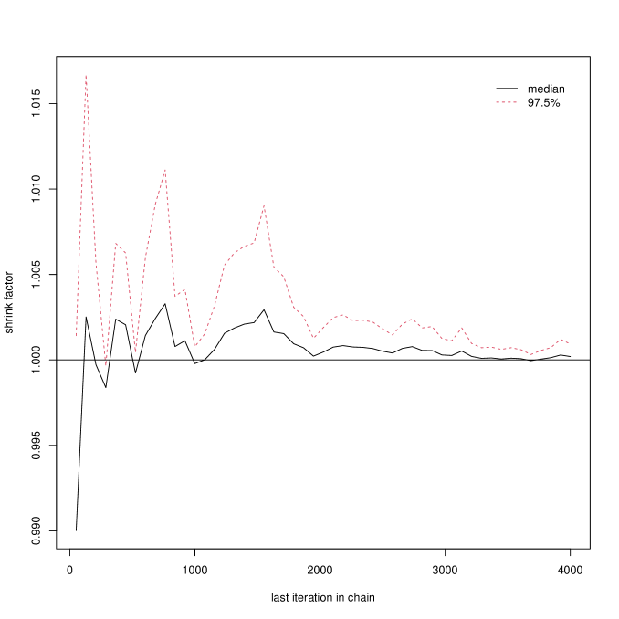
Figure S2: Plot of potential scale reduction factors in one randomly selected Monte Carlo replicate in simulation studies for 5 different MCMC with 1000 burn-in samples and 4000 post-burn-in samples.

Appendix F Implementation Details of Competitors in Simulation Studies

Four competitors are considered in the simulation studies: principal cluster analysis K-means (PCA-KM), sparse K-means (SKM) (Witten and Tibshirani,, 2010), Clustering of High-dimensional Gaussian Mixtures with the Expectation-Maximization (CHIME), and Gaussian-mixture-model-based clustering (MClust) (Fraley et al.,, 2012). In particular, PCA-KM is a two-stage approach that first performs a PCA to reduce dimensionality and then applies a K-means algorithm to the principal clusters. SKM is a generalization of the K-means in high dimensions to find clusters and important features (i.e., the non-zero coordinates) simultaneously. CHIME is a high-dimensional clustering approach based on an EM algorithm. To overcome the issue that the sample covariance matrix may not be invertible and thus the subsequent estimate of $z$ is not available, CHIME focuses on the so-called sparse discriminant vector and directly use it in the Fisher discriminant rule to estimate cluster memberships. Note that the performance of CHIME is quite sensitive to the choice of initial values. Throughout simulation examples, we set the initial values of CHIME to be the output of K-means. For PCA-KM and SKM, we choose the number of clusters via Silhouette method (Rousseeuw,, 1987), with the range of $K$ being from 2 to 10. For MClust and CHIME, the number of clusters is estimated via Bayesian information criterion.

Appendix G Additional Numerical Results in Simulation Studies

This section provides additional numerical results in simulation studies. Note that the evaluation of clustering accuracy is based on the adjusted Rand index (Rand,, 1971), defined as follows. Let $\mathcal{C}^{*}$ and $\mathcal{C}^{\dagger}$ denote the true and estimated partition of $[n]$, respectively, and let $K^{*}\overset{\Delta}{=}|\mathcal{C}^{*}|$, $K^{\dagger}\overset{\Delta}{=}|\mathcal{C}^{\dagger}|$. For each cluster, denote $n^{*}_{k}$ to be the size of $k$th cluster in $\mathcal{C}^{*}$ and $n^{\dagger}_{k^{\prime}}$ as the size of $k^{\prime}$th cluster in $\mathcal{C}^{\dagger}$. Furthermore, let $n_{k,k^{\prime}}$ be the number of observations that are assigned to both the $k$th cluster in $\mathcal{C}^{*}$ and $k^{\prime}$th cluster in $\mathcal{C}^{\dagger}$. Then the adjusted Rand index is defined as

$$\mathrm{ARI}(\mathcal{C}^{*},\mathcal{C}^{\dagger})=\frac{\sum_{k=1}^{K^{*}}\sum_{k^{\prime}=1}^{K^{\dagger}}{n_{k,k^{\prime}}\choose 2}-\sum_{k=1}^{K^{*}}{n_{k}\choose 2}\sum_{k^{\prime}=1}^{K^{\dagger}}{n_{k^{\prime}}\choose 2}/{n\choose 2}}{\left(\sum_{k=1}^{K_{t}}{n_{k}\choose 2}+\sum_{k^{\prime}=1}^{K^{\dagger}}{n_{k^{\prime}}\choose 2}\right)/2-\sum_{k=1}^{K^{*}}{n_{k}\choose 2}\sum_{k^{\prime}=1}^{K^{\dagger}}{n_{k^{\prime}}\choose 2}/{n\choose 2}}.$$

Scenario I: We first provide some detailed results when $K^{*}=5$. In particular, PCA-KM, SKM, MClust, and CHIME only correctly estimate the number of clusters in 6, 0, 4, and 3 out of 100 replicates for s = 6, and in 8, 0, 9, and 3 out of 100 replicates for s = 12. Figure S3 plots the simulated true cluster memberships and the estimated clustering results under the proposed Bayesian method and the four competitors for one randomly selected simulation replicate when $K^{*}=5$, $s=6$. Similarly as the case when $K^{*}=3$, the four competitors cannot well distinguish the overlapping clusters, i.e., the purple and blue clusters in the upper left panel of Figure S3, while the proposed Bayesian method can successfully separate them.

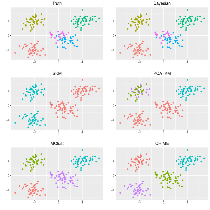
Figure S3: Clustering results of different methods compared with the true cluster memberships for the simulation scenario I with $K^{*}=5$ and $s=6$ in a randomly selected simulation replicate. Data points are projected onto the subspace of the first two coordinates and different colors correspond to different estimated cluster memberships of the data points.

Moreover, we provide a detailed histogram of the estimated number of clusters under all methods in Figure S4, which shows that the proposed Bayesian method successfully recovers the simulated true numbers of clusters while all the four competitors underestimate them.

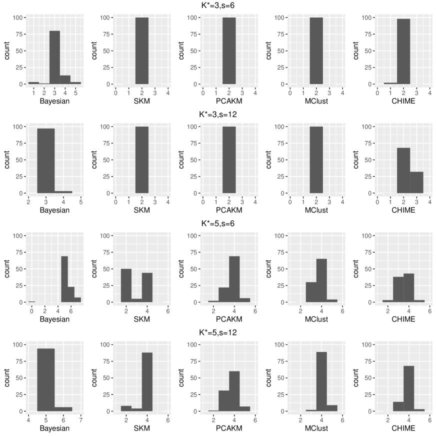
Figure S4: Histograms of estimated number of clusters under different methods in scenario I of simulation studies.

In terms of cluster-wise mean vector estimation accuracy, Figure S5 presents the boxplots of $\|\hat{\bm{\mu}}_{1}-\bm{\mu}^{*}_{1}\|_{2}$ when $K^{*}=3$ and $s=12$ across 100 simulation replicates under different methods, showing that the proposed Bayesian method yields the smallest error of estimating $\bm{\mu}^{*}_{1}$.

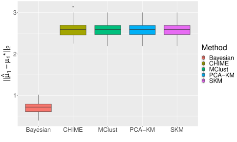
Figure S5: Numerical results of $\|\hat{\bm{\mu}}_{1}-\bm{\mu}^{*}_{1}\|_{2}$ of different methods in scenario I with $K^{*}=3$ and $s=12$ across 100 simulation replicates.

Furthermore, Figure S6 indicates that the proposed Bayesian method recovers the sparsity pattern better than the four competitors.

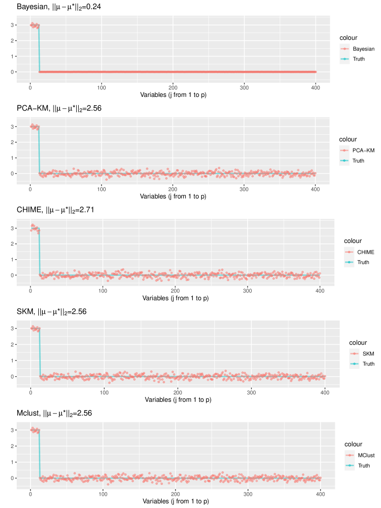
Figure S6: Estimation of mean vector $\bm{\mu}_{1}^{*}$ of different methods in scenario I with $K^{*}=3$ and $s=12$ in a randomly selected simulation replicate.

Scenario III: In this scenario, we present the histograms of the estimated number of clusters under different methods in Figure S7. In addition, Figure S8 visualizes the clustering results under different methods in a randomly selected simulation replicate. Note that the multivariate $t$-distribution is heavy-tailed. Since we mis-specify the working model as Gaussian mixtures, it is reasonable to treat some observations as “outliers”, as shown in the upper left panel of Figure S8. Therefore, the proposed Bayesian method tends to assign these “outliers” to small clusters when it overestimates the number of clusters. The proposed Bayesian method successfully identifies three clusters in 76 out of 100 simulation replicates, with an average ARI of 0.97 across 100 simulation replicates. PCA-KM returns 10 clusters in 59 out of 100 simulation replicates with the average ARI being 0.84. The estimated numbers of clusters of SKM are all 2 in 100 simulation replicates, and the average ARI is 0.52. For model-based methods, i.e., MClust and CHIME, which also utilize Gaussian mixtures as the working likelihood, their performance are much worse than others as they only identify one cluster in 93 out of 100 replicates, resulting in the average ARIs less than 0.05.

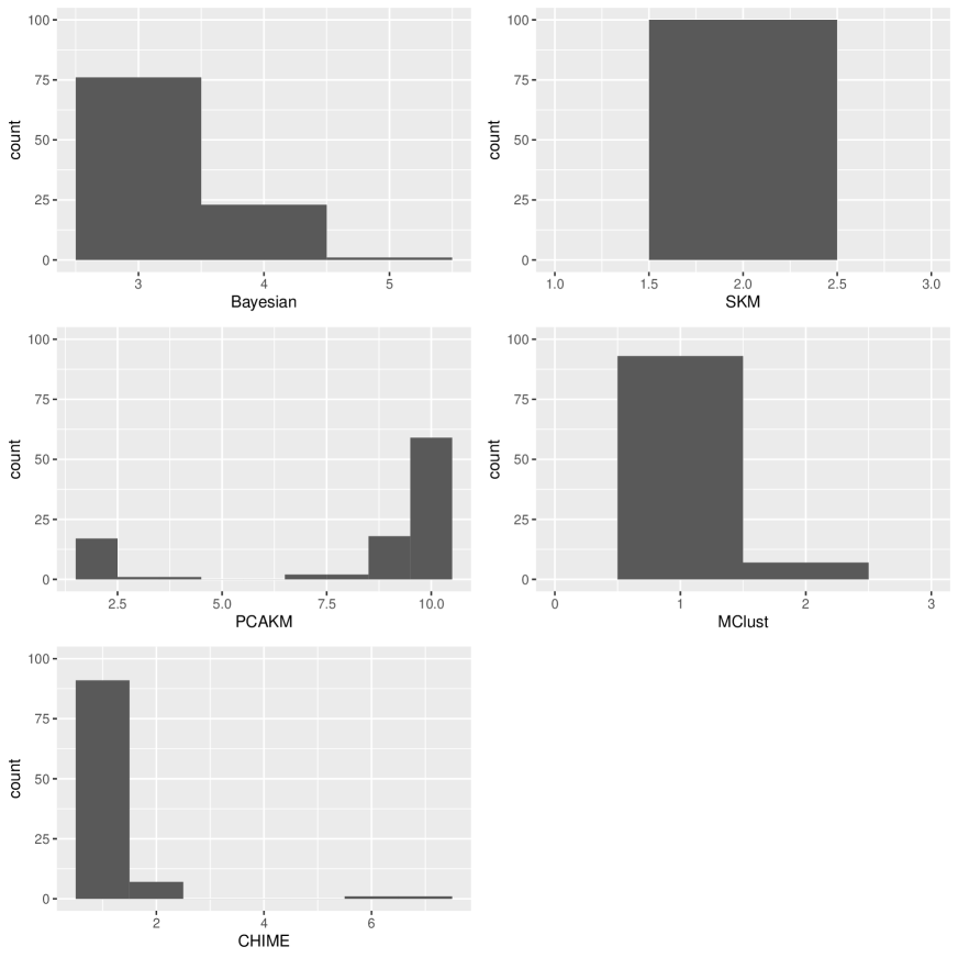
Figure S7: Histograms of estimated number of clusters under different methods in scenario III of simulation studies.

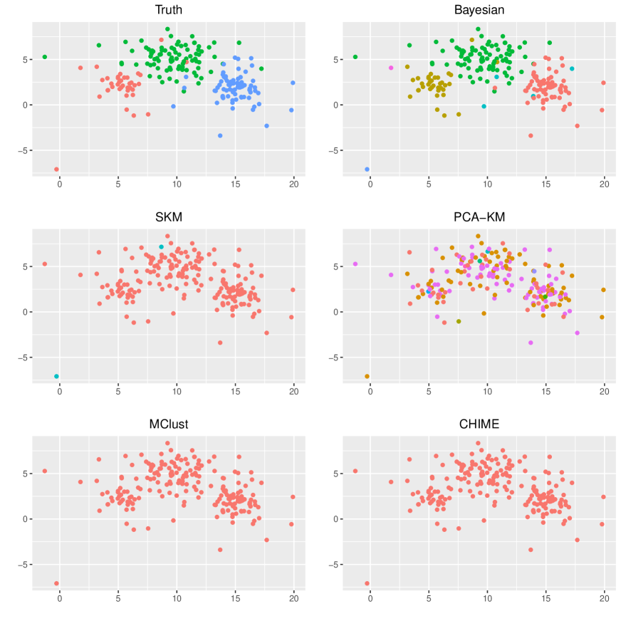
Figure S8: Clustering results under different methods in one randomly selected replicate of scenario III. Data points are projected onto the subspace of the first two coordinates and different colors correspond to different estimated cluster memberships of the data points.

Appendix H Additional Numerical Results in Single-cell Sequencing Data Analysis

In this section, we provide more numerical results in section 5, including the clustering results of alternative methods when the number of clusters is set to be the truth in Figure S9 and the corresponding adjusted Rand indices and normalized mutual information in Table S1. Note that the evaluation of clustering accuracy is not only based on the adjusted Rand index, but also the normalized mutual information (Ghosh and Acharya,, 2011). Similarly as the definition of adjusted Rand index, let $\mathcal{C}^{*}$ and $\mathcal{C}^{\dagger}$ denote the true and estimated partition of $[n]$, respectively, and let $K^{*}\overset{\Delta}{=}|\mathcal{C}^{*}|$, $K^{\dagger}\overset{\Delta}{=}|\mathcal{C}^{\dagger}|$. For each cluster, denote $n^{*}_{k}$ to be the size of $k$th cluster in $\mathcal{C}^{*}$ and $n^{\dagger}_{k^{\prime}}$ as the size of $k^{\prime}$th cluster in $\mathcal{C}^{\dagger}$. Furthermore, let $n_{k,k^{\prime}}$ be the number of observations that are assigned to both the $k$th cluster in $\mathcal{C}^{*}$ and $k^{\prime}$th cluster in $\mathcal{C}^{\dagger}$. Then the normalized mutual information is defined as

$$\text{NMI}(\mathcal{C}^{*},\mathcal{C}^{\dagger})=\frac{\sum_{k=1}^{K^{*}}\sum_{k^{\prime}=1}^{K^{\dagger}}\frac{n_{k,k^{\prime}}}{n}\log\left(\frac{n_{k,k^{\prime}}}{n}\right)-\sum_{k=1}^{K^{*}}\frac{n_{k}^{*}}{n}-\sum_{k^{\prime}=1}^{K^{\dagger}}\frac{n_{k^{\prime}}^{\dagger}}{n}\log\left(\frac{n_{k^{\prime}}^{\dagger}}{n}\right)}{\sqrt{\sum_{k=1}^{K^{*}}\frac{n_{k}^{*}}{n}\log\left(\frac{n_{k}^{*}}{n}\right)\sum_{k=1}^{K^{\dagger}}\frac{n_{k^{\prime}}^{\dagger}}{n}\log\left(\frac{n_{k^{\prime}}^{\dagger}}{n}\right)}}.$$

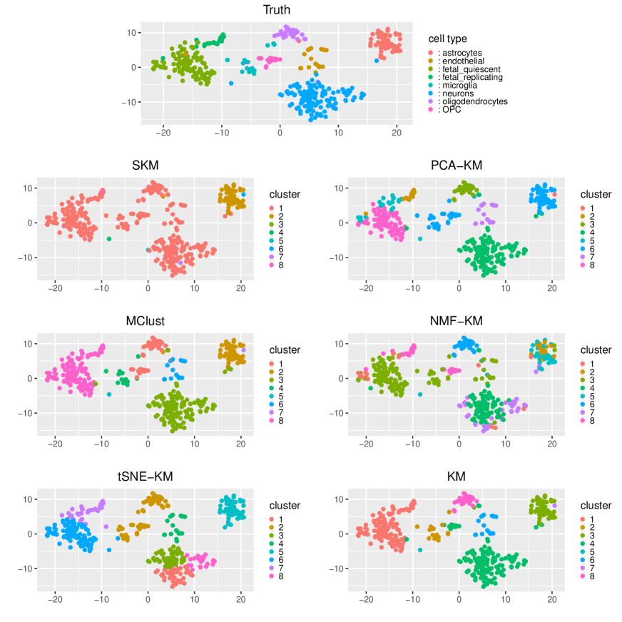
Figure S9: Clustering results of scRNA-Seq data corresponding to alternative methods. The number of clusters is set to be truth ($K=8$) for all methods.

Methods	ARI	NMI
KM	0.79	0.77
tSNE-KM	0.63	0.73
PCA-KM	0.81	0.79
NMF-KM	0.77	0.78
SKM	0.15	0.23
MClust	0.83	0.79

Table S1: ARIs and NMIs of different methods on scRNA-Seq data. The number of clusters is set to be truth ($K=8$) for all methods.

References

• Agterberg et al., (2022) Agterberg, J., Lubberts, Z., and Priebe, C. E. (2022). Entrywise estimation of singular vectors of low-rank matrices with heteroskedasticity and dependence. IEEE Transactions on Information Theory, 68(7):4618–4650.
• Ashtiani et al., (2020) Ashtiani, H., Ben-David, S., Harvey, N. J., Liaw, C., Mehrabian, A., and Plan, Y. (2020). Near-optimal sample complexity bounds for robust learning of gaussian mixtures via compression schemes. Journal of the ACM (JACM), 67(6):1–42.
• Azizyan et al., (2013) Azizyan, M., Singh, A., and Wasserman, L. (2013). Minimax theory for high-dimensional Gaussian mixtures with sparse mean separation. Advances in Neural Information Processing Systems, 26.
• Bai et al., (2021) Bai, R., Ročková, V., and George, E. I. (2021). Spike-and-slab meets lasso: A review of the spike-and-slab lasso. Handbook of Bayesian Variable Selection, pages 81–108.
• Bhattacharya et al., (2015) Bhattacharya, A., Pati, D., Pillai, N. S., and Dunson, D. B. (2015). Dirichlet–Laplace priors for optimal shrinkage. Journal of the American Statistical Association, 110(512):1479–1490. PMID: 27019543.
• Blei et al., (2003) Blei, D. M., Ng, A. Y., and Jordan, M. I. (2003). Latent Dirichlet allocation. Journal of machine Learning research, 3(Jan):993–1022.
• Brooks and Gelman, (1998) Brooks, S. P. and Gelman, A. (1998). General methods for monitoring convergence of iterative simulations. Journal of computational and graphical statistics, 7(4):434–455.
• Cai et al., (2019) Cai, T. T., Ma, J., and Zhang, L. (2019). CHIME: Clustering of high-dimensional Gaussian mixtures with EM algorithm and its optimality. The Annals of Statistics, 47(3):1234 – 1267.
• Cai et al., (2016) Cai, T. T., Ren, Z., and Zhou, H. H. (2016). Estimating structured high-dimensional covariance and precision matrices: Optimal rates and adaptive estimation. Electronic Journal of Statistics, 10(1):1 – 59.
• Cao et al., (2019) Cao, J., Spielmann, M., Qiu, X., Huang, X., Ibrahim, D. M., Hill, A. J., Zhang, F., Mundlos, S., Christiansen, L., Steemers, F. J., et al. (2019). The single-cell transcriptional landscape of mammalian organogenesis. Nature, 566(7745):496–502.
• Cape et al., (2018) Cape, J., Tang, M., and Priebe, C. (2018). Signal-plus-noise matrix models: Eigenvector deviations and fluctuations. Biometrika, 106.
• Carvalho et al., (2009) Carvalho, C., Polson, N., and Scott, J. (2009). Handling sparsity via the Horseshoe. Journal of Machine Learning Research - Proceedings Track, 5:73–80.
• Castillo et al., (2015) Castillo, I., Schmidt-Hieber, J., and van der Vaart, A. (2015). Bayesian linear regression with sparse priors. The Annals of Statistics, 43(5):1986 – 2018.
• Castillo and van der Vaart, (2012) Castillo, I. and van der Vaart, A. (2012). Needles and Straw in a Haystack: Posterior concentration for possibly sparse sequences. The Annals of Statistics, 40(4):2069 – 2101.
• Chandra et al., (2022) Chandra, N. K., Canale, A., and Dunson, D. B. (2022). Escaping the curse of dimensionality in Bayesian model based clustering. arXiv preprint arXiv:2006.02700.
• Darmanis et al., (2015) Darmanis, S., Sloan, S. A., Zhang, Y., Enge, M., Caneda, C., Shuer, L. M., Gephart, M. G. H., Barres, B. A., and Quake, S. R. (2015). A survey of human brain transcriptome diversity at the single cell level. Proceedings of the National Academy of Sciences, 112(23):7285–7290.
• Diday et al., (1981) Diday, E., Govaert, G., Lechevallier, Y., and Sidi, J. (1981). Clustering in pattern recognition. In Digital Image Processing, pages 19–58. Springer.
• Ding et al., (2002) Ding, C., He, X., Zha, H., and Simon, H. D. (2002). Adaptive dimension reduction for clustering high dimensional data. In 2002 IEEE International Conference on Data Mining, 2002. Proceedings., pages 147–154. IEEE.
• Doss et al., (2021) Doss, N., Wu, Y., Yang, P., and Zhou, H. H. (2021). Optimal estimation of high-dimensional location Gaussian mixtures. arXiv preprint arXiv:2002.05818.
• Fraley et al., (2012) Fraley, C., Raftery, A., Murphy, T., and Scrucca, L. (2012). MCLUST Version 4 for R: Normal Mixture Modeling for Model-Based Clustering, Classification, and Density Estimation. Technical Report No. 597.
• Fraley and Raftery, (2002) Fraley, C. and Raftery, A. E. (2002). Model-based clustering, discriminant analysis, and density estimation. Journal of the American Statistical Association, 97(458):611–631.
• Georghiades et al., (2001) Georghiades, A., Belhumeur, P., and Kriegman, D. (2001). From few to many: Illumination cone models for face recognition under variable lighting and pose. IEEE Trans. Pattern Anal. Mach. Intelligence, 23(6):643–660.
• Ghosal et al., (2000) Ghosal, S., Ghosh, J. K., and van der Vaart, A. W. (2000). Convergence rates of posterior distributions. The Annals of Statistics, 28(2):500 – 531.
• Ghosh and Acharya, (2011) Ghosh, J. and Acharya, A. (2011). Cluster ensembles. Wiley interdisciplinary reviews: Data mining and knowledge discovery, 1(4):305–315.
• Ghosh et al., (2020) Ghosh, P., Pati, D., and Bhattacharya, A. (2020). Posterior contraction rates for stochastic block models. Sankhya A, 82(2):448–476.
• Green, (1995) Green, P. J. (1995). Reversible jump Markov chain Monte Carlo computation and Bayesian model determination. Biometrika, 82(4):711–732.
• Gu and Liu, (2008) Gu, J. and Liu, J. S. (2008). Bayesian biclustering of gene expression data. BMC genomics, 9(1):1–10.
• Hagerup and Rüb, (1990) Hagerup, T. and Rüb, C. (1990). A guided tour of chernoff bounds. Information processing letters, 33(6):305–308.
• Jin et al., (2017) Jin, J., Ke, Z. T., and Wang, W. (2017). Phase transitions for high dimensional clustering and related problems. The Annals of Statistics, 45(5):2151–2189.
• Jin and Wang, (2016) Jin, J. and Wang, W. (2016). Influential features PCA for high dimensional clustering. The Annals of Statistics, 44(6):2323 – 2359.
• Johnstone and Lu, (2009) Johnstone, I. M. and Lu, A. Y. (2009). On consistency and sparsity for principal components analysis in high dimensions. Journal of the American Statistical Association, 104(486):682–693. PMID: 20617121.
• Kosorok, (2008) Kosorok, M. (2008). Introduction to Empirical Processes and Semiparametric Inference.
• Löffler et al., (2021) Löffler, M., Zhang, A. Y., and Zhou, H. H. (2021). Optimality of spectral clustering in the Gaussian mixture model. The Annals of Statistics, 49(5):2506–2530.
• Luxburg, (2004) Luxburg, U. (2004). A tutorial on spectral clustering. Statistics and Computing, 17:395–416.
• Massart, (2007) Massart, P. (2007). Concentration inequalities and model selection. ecole d’eté de probabilités de saint-flour xxxiii – 2003. Lecture Notes in Mathematics -Springer-verlag-, 1896.
• Miller, (2018) Miller, J. W. (2018). A detailed treatment of Doob’s theorem. arXiv:1801.03122.
• Miller and Harrison, (2018) Miller, J. W. and Harrison, M. T. (2018). Mixture models with a prior on the number of components. Journal of the American Statistical Association, 113(521):340–356.
• Mitchell and Beauchamp, (1988) Mitchell, T. J. and Beauchamp, J. J. (1988). Bayesian variable selection in linear regression. Journal of the American Statistical Association, 83(404):1023–1032.
• Natalini and Palumbo, (2000) Natalini, P. and Palumbo, B. (2000). Inequalities for the incomplete gamma function. Math. Inequal. Appl, 3(1):69–77.
• Ohn and Lin, (2022) Ohn, I. and Lin, L. (2022). Optimal Bayesian estimation of Gaussian mixtures with growing number of components. arXiv preprint arXiv:2007.09284.
• Rand, (1971) Rand, W. M. (1971). Objective criteria for the evaluation of clustering methods. Journal of the American Statistical Association, 66(336):846–850.
• Ray and Szabó, (2021) Ray, K. and Szabó, B. (2021). Variational bayes for high-dimensional linear regression with sparse priors. Journal of the American Statistical Association, pages 1–12.
• Ročková and George, (2018) Ročková, V. and George, E. I. (2018). The spike-and-slab lasso. Journal of the American Statistical Association, 113(521):431–444.
• Rousseeuw, (1987) Rousseeuw, P. J. (1987). Silhouettes: A graphical aid to the interpretation and validation of cluster analysis. Journal of Computational and Applied Mathematics, 20:53–65.
• Smyth, (2000) Smyth, P. (2000). Model selection for probabilistic clustering using cross-validated likelihood. Statistics and computing, 10(1):63–72.
• Tadesse et al., (2005) Tadesse, M. G., Sha, N., and Vannucci, M. (2005). Bayesian variable selection in clustering high-dimensional data. Journal of the American Statistical Association, 100(470):602–617.
• Tadesse and Vannucci, (2021) Tadesse, M. G. and Vannucci, M. (2021). Handbook of Bayesian variable selection.
• Tibshirani et al., (2001) Tibshirani, R., Walther, G., and Hastie, T. (2001). Estimating the number of clusters in a data set via the gap statistic. Journal of the Royal Statistical Society: Series B (Statistical Methodology), 63(2):411–423.
• Van der Maaten and Hinton, (2008) Van der Maaten, L. and Hinton, G. (2008). Visualizing data using t-sne. Journal of machine learning research, 9(11).
• Witten and Tibshirani, (2010) Witten, D. M. and Tibshirani, R. (2010). A framework for feature selection in clustering. Journal of the American Statistical Association, 105(490):713–726.
• Xie et al., (2022) Xie, F., Cape, J., Priebe, C. E., and Xu, Y. (2022). Bayesian sparse spiked covariance model with a continuous matrix shrinkage prior. Bayesian Analysis, 1(1):1–25.
• Yang et al., (2016) Yang, D., Ma, Z., and Buja, A. (2016). Rate optimal denoising of simultaneously sparse and low rank matrices. Journal of Machine Learning Research, 17(92):1–27.
• (53) Yu, Y., Wang, T., and Samworth, R. J. (2014a). A useful variant of the Davis–Kahan theorem for statisticians. Biometrika, 102(2):315–323.
• (54) Yu, Y., Wang, T., and Samworth, R. J. (2014b). A useful variant of the Davis–Kahan theorem for statisticians. Biometrika, 102(2):315–323.
• Zhu et al., (2017) Zhu, X., Ching, T., Pan, X., Weissman, S. M., and Garmire, L. (2017). Detecting heterogeneity in single-cell RNA-Seq data by non-negative matrix factorization. PeerJ, 5:e2888.