Abstract

This paper proposes a new loss function for adversarial training. Since adversarial training has difficulties, e.g., necessity of high model capacity, focusing on important data points by weighting cross-entropy loss has attracted much attention. However, they are vulnerable to sophisticated attacks, e.g., Auto-Attack. This paper experimentally reveals that the cause of their vulnerability is their small margins between logits for the true label and the other labels. Since neural networks classify the data points based on the logits, logit margins should be large enough to avoid flipping the largest logit by the attacks. Importance-aware methods do not increase logit margins of important samples but decrease those of less-important samples compared with cross-entropy loss. To increase logit margins of important samples, we propose switching one-vs-the-rest loss (SOVR), which switches from cross-entropy to one-vs-the-rest loss for important samples that have small logit margins. We prove that one-vs-the-rest loss increases logit margins two times larger than the weighted cross-entropy loss for a simple problem. We experimentally confirm that SOVR increases logit margins of important samples unlike existing methods and achieves better robustness against Auto-Attack than importance-aware methods.

1 Introduction

For multi-class classification problems, deep neural networks have become the de facto standard method in this decade. They classify a data point into the label that has the largest logit, which is the input of a softmax function. However, the largest logit is easily flipped, and deep neural networks can misclassify slightly perturbed data points, which are called adversarial examples (Szegedy et al., 2013). Various methods have been presented to search the adversarial examples, and Auto-Attack (Croce & Hein, 2020) is one of the most successful methods at finding the worst-case attacks. For trustworthy deep learning applications, classifiers should be robust against the worst-case attacks. To improve the robustness, many defense methods have also been presented (Kurakin et al., 2016; Madry et al., 2018; Wang et al., 2020b; Cohen et al., 2019). Among them, adversarial training is a promising method, which empirically achieves good robustness (Carmon et al., 2019; Kurakin et al., 2016; Madry et al., 2018). However, adversarial training is more difficult than standard training, e.g., it requires higher sample complexity (Schmidt et al., 2018; Wang et al., 2020a) and model capacity (Zhang et al., 2021b).

To address these difficulties, several methods focus on the difference in importance of data points (Wang et al., 2020a; Liu et al., 2021; Zhang et al., 2021b). These studies hypothesize that data points closer to a decision boundary are more important for adversarial training (Wang et al., 2020a; Zhang et al., 2021b; Liu et al., 2021). To focus on such data points, GAIRAT (Zhang et al., 2021b) and MAIL (Liu et al., 2021) use weighted softmax cross-entropy loss, which controls weights on the losses on the basis of the closeness to the boundary. As the measure of the closeness, GAIRAT uses the least number of steps at which the iterative attacks make models misclassify the data point. On the other hand, MAIL uses the measure based on the softmax outputs. However, these importance-aware methods tend to be more vulnerable to the robustness against Auto-Attack than naïve adversarial training. Thus, it is still unclear whether focusing on the important training data points enhances the robustness in adversarial training.

To answer this question, we investigate the cause of the vulnerability of importance-aware methods via margins between logits for the true label and the other labels. Since neural networks classify the data into the largest logit class, logit margins should be large enough to avoid the flipping of the largest logit class by the attacks. Through the histogram of logit margins, we first confirmed that there is actually a difference in the data points when using naïve adversarial training (AT). AT has two peaks in the histogram, i.e., large and small logit margins. This indicates that there are difficult samples of which logit margins are difficult to be increased, and they correspond to important samples since small logit margins indicate that data points are near the decision boundary. Next, we found that importance-aware methods only have one peak of small logit margins near zero in the histogram. Thus, importance-aware methods do not increase logit margins of important samples but decrease the logit margins of easy (less-important) samples. As a result, importance-aware methods are more vulnerable near less-important samples than AT. This implies that weighting cross-entropy used in importance-aware methods is not very effective strategy for focussing on important samples.

To increase the logit margins of important samples, we propose switching one-vs-the-rest loss (SOVR), which switches between cross-entropy and one-vs-the-rest loss (OVR) for less-important and important samples, instead of weighting cross-entropy. We prove that OVR is always greater than or equal to cross-entropy on any logits. Furthermore, we theoretically derive the trajectories of logit margin losses in minimizing OVR and cross-entropy by using gradient flow on a simple problem. These trajectories reveal that OVR increases logit margins two times larger than weighted cross-entropy losses after sufficient training time. Thus, SOVR increases logit margins of important samples while it does not decrease logit margins of less-important, unlike importance-aware methods. Experiments demonstrate that SOVR increases logit margins more than AT and outperforms AT, GAIRAT (Zhang et al., 2021b), MAIL (Liu et al., 2021), MART (Wang et al., 2020a), MMA (Ding et al., 2020), and EWAT (Kim et al., 2021) in terms of robustness against Auto-Attack. In addition, we find that SOVR achieves a better trade-off than TRADES, and the combination of SOVR and TRADES achieves the best robustness. Thus, focusing on important data points improves the robustness when increasing their logit margins by OVR. Furthermore, our method improves the performance of other recent optimization methods (Wu et al., 2020; Wang & Wang, 2022) and data augmentation using 1M synthetic data (Rebuffi et al., 2021; Gowal et al., 2021) for adversarial training.

2 Preliminaries

2.1 Adversarial Training

Given $N$ data points $\bm{x}_{n}\!\in\!\mathbb{R}^{d}$ and class labels $y_{n}\!\in\!\{1,\dots,K\}$, adversarial training (Madry et al., 2018) attempts to solve the following minimax problem with respect to the model parameter $\bm{\theta}\!\in\!\mathbb{R}^{m}$:

$$\textstyle\min_{\bm{\theta}}\mathcal{L}_{\mathrm{AT}}(\bm{\theta})=\textstyle\min_{\bm{\theta}}\frac{1}{N}\sum_{n=1}^{N}\ell_{\mathrm{CE}}(\bm{z}(\bm{x}_{n}^{\prime},\!\bm{\theta}),\!y_{n}),$$ (1)

$$\textstyle\bm{x}_{n}^{\prime}\textstyle=\bm{x}_{n}\!+\!\bm{\delta}_{n}$$

$$~{}~{}~{}\textstyle=\!\bm{x}_{n}\!+\!\mathrm{arg}\!\max_{|\!|\bm{\delta}_{n}|\!|_{p}\leq\varepsilon}\ell_{\mathrm{CE}}(\bm{z}(\bm{x}_{n}\!+\!\bm{\delta}_{n},\bm{\theta}),\!y_{n}),$$ (2)

where $\bm{z}(\bm{x},\bm{\theta})\!=\![z_{1}(\bm{x},\bm{\theta}),\dots,z_{K}(\bm{x},\bm{\theta})]^{T}$ and $z_{k}(\bm{x},\bm{\theta})$ is the $k$-th logit of the model, which is input of softmax:$f_{k}(\bm{x},\bm{\theta})\!=\!e^{z_{k}(\bm{x})}\!/\!\sum_{i}e^{z_{i}(\bm{x})}$. $\ell_{\mathrm{CE}}$ is a cross-entropy function, and $||\cdot||_{p}$ and $\varepsilon$ are $L_{p}$ norm and the magnitude of perturbation $\bm{\delta}_{n}\!\in\!\mathbb{R}^{d}$, respectively. The inner maximization problem is solved by projected gradient descent (PGD) (Kurakin et al., 2016; Madry et al., 2018), which updates the adversarial examples as

$$\textstyle\!\!\!\!\bm{\delta}_{t}\!=\!\Pi_{\varepsilon}\!\left(\bm{\delta}\!+\!\eta\mathrm{sign}\left(\nabla_{\bm{\delta}_{t-1}}\!\ell_{\mathrm{CE}}\left(\bm{z}(\bm{x}\!+\!\bm{\delta}_{t-1},\bm{\theta}),y\right)\!\right)\!\right),$$ (3)

for $\mathcal{K}$ steps where $\eta$ is a step size. $\Pi_{\varepsilon}$ is a projection operation into the feasible region $\{\bm{\delta}~{}|~{}\bm{\delta}\in\mathbb{R}^{d},||\bm{\delta}||_{p}\leq\varepsilon\}$. Note that we focus on $p\!=\!\infty$ since it is a common setting. For trustworthy deep learning, we should improve the true robustness: the robustness against the worst-case attacks in the feasible region. Thus, the evaluation of robustness should use crafted attacks, e.g., Auto-Attack (Croce & Hein, 2020), since PGD often fails to find the adversarial examples misclassified by models.

2.2 Importance-aware Adversarial Training

GAIRAT (geometry aware instance reweighted adversarial training) (Zhang et al., 2021b) and MAIL (margin-aware instance reweighting learning) (Liu et al., 2021) regard data points closer to the decision boundary of model $\bm{f}$ as important samples and assign higher weights to the loss for them:

$$\textstyle\mathcal{L}_{\mathrm{weight}}(\bm{\theta})=\textstyle\frac{1}{N}\sum_{n=1}^{N}\bar{w}_{n}\ell_{\mathrm{CE}}(\bm{z}(\bm{x}_{n}^{\prime},\bm{\theta}),\!y_{n}),$$ (4)

where $\bar{w}_{n}\!\geq\!0$ is a weight normalized as $\bar{w}_{n}\!=\!\frac{w_{n}}{\sum_{l}{w}_{l}}$ and $\sum_{n}\bar{w}_{n}\!=\!1$. GAIRAT determines the weights through the $w_{n}\!=\!\frac{1\!+\!\mathrm{tanh}(\lambda+5(1-2\kappa_{n}/\mathcal{K}))}{2}$ where $\kappa_{n}$ is the least steps at which PGD succeeds at attacking models, and $\lambda$ is a hyperparameter. On the other hand, MAIL uses $w_{n}\!=\!\mathrm{sigmoid}(-\gamma(PM_{n}\!-\!\beta))$ where $PM_{n}\!=\!f_{y_{n}}(\bm{x}_{n}^{\prime},\bm{\theta})\!-\!\max_{k\neq{y_{n}}}f_{k}(\bm{x}_{n}^{\prime},\bm{\theta})$. $\beta$ and $\gamma$ are hyperparameters. MART (misclassification aware adversarial training) (Wang et al., 2020a) uses a similar approach. It regards misclassified samples as important samples and controls the difference between the loss on less-important and important samples. MMA (max-margin adversarial training) (Ding et al., 2020) also adaptively changes the loss function and $\varepsilon$ for each data point, and thus, MMA also has a similar effect to the above methods. We collectively call the above methods importance-aware methods.

2.3 Vulnerability of Importance-aware Methods

Hitaj et al. (2021); Croce & Hein (2020); Kim et al. (2021) have reported that the robust accuracies of GAIRAT, MART, and MMA are lower than naïve adversarial training when using logit scaling attacks or Auto-Attack (Croce & Hein, 2020). Since Auto-Attack searches adversarial examples by using various attacks, it achieves a larger success attack rate than using one attack, e.g., PGD. To clarify the vulnerabilities, we individually evaluate the robustness against the components of Auto-Attack and PGD ($\mathcal{K}\!=\!20$) on CIFAR10 (Fig. 1). The training setup is the same as in Section 6, and we add the results of our method (SOVR) as a reference. This figure shows that almost all importance-aware methods can improve the robustness against PGD and APGD compared with naïve adversarial training (AT (Madry et al., 2018)). However, they do not improve the true robustness; i.e., their robust accuracies against the worst-case attack are lower than that of AT. We investigate the reasons of this vulnerability in the next section.

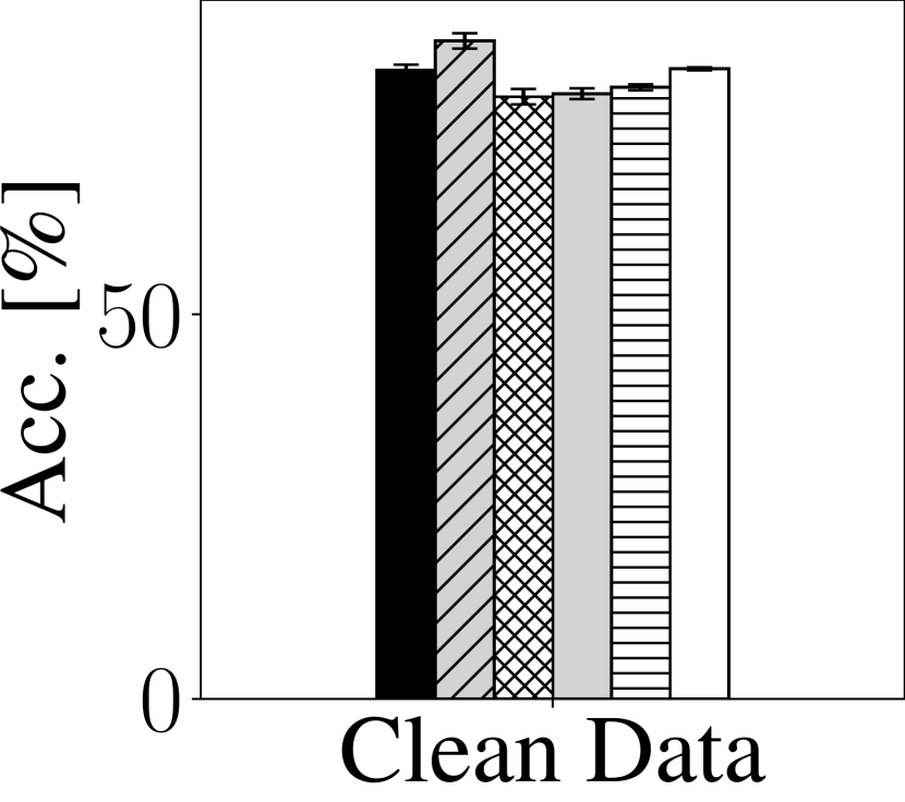
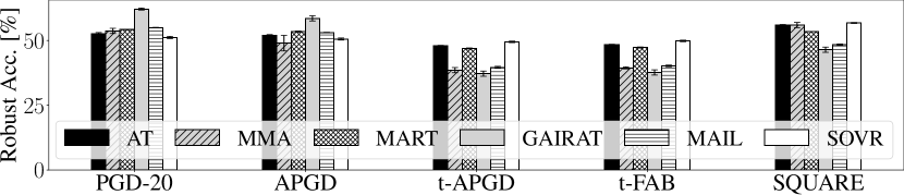
Figure 1: Robustness against PGD and components of Auto-Attack on CIFAR10 (Krizhevsky & Hinton, 2009) with PreActResNet18 (RN18). SOVR is our proposed method.

3 Evaluation of Robustness via Logit Margin

We investigate the causes of the vulnerabilities of importance-aware methods by comparing histograms of logit margin losses. First, we explain that logit margin losses determine the robustness. Next, we experimentally reveal that logit margin losses of importance-aware methods concentrate on zero; i.e., their logit margins are smaller than AT. We use training data for empirical evaluation in this section because the goal of this section is to investigate the effect of importance-aware methods, which modify the loss function based on training data points. Experimental setups are provided in Appendix E.6.

3.1 Potentially Misclassified Data Detected by Logit Margin Loss

To investigate the robustness of models near each data point, we apply logit margin loss (Ding et al., 2020) to the models trained by importance-aware methods. Logit margin loss is

$$\textstyle\ell_{\mathrm{LM}}(\bm{z}(\bm{x}_{n},\bm{\theta}),y) \textstyle=z_{k^{*}}(\bm{x}^{\prime})-z_{y_{n}}(\bm{x}^{\prime})$$

$$\textstyle=\max_{k\neq y}z_{k}(\bm{x}^{\prime})-z_{y}(\bm{x}^{\prime}),$$ (5)

where $k^{*}\!=\!\mathrm{arg}\!\max_{k\neq y}\!z_{k}(\bm{x}^{\prime})$. Since the classifier infers the label of $\bm{x}$ as $\hat{y}\!=\!\mathrm{arg}\!\max_{k}\!z_{k}(\bm{x})$, it correctly classifies $\bm{x}^{\prime}$ if $\ell_{\mathrm{LM}}\leq 0$. Thus, the logit margin loss on a difficult sample in adversarial training takes a value near zero. We refer to the absolute value of a logit margin loss $|\ell_{\mathrm{LM}}|$ as logit margin. In contrast to $\mathrm{PM}_{n}$ of MAIL, $\ell_{\mathrm{LM}}$ is not bounded since $z_{k}(\bm{x})$ can take an arbitrary value in $\mathbb{R}$.

To explain the effect of logit margins, we assume that the Lipschitz constant of the $k$-th logit function is $L_{k}$ as $|z_{k}(\bm{x}_{1})\!-\!z_{k}(\bm{x}_{2})|\!\leq\!L_{k}||\bm{x}_{1}-\bm{x}_{2}||_{\infty}$. In this case, we have the following inequality:

$$\textstyle\max_{k}\!z_{k}(\bm{x}^{\prime})\!-\!z_{y}(\bm{x}^{\prime}) \!\textstyle\!\leq\!\max_{k}\!\left[\textstyle z_{k}(\bm{x})\!-\!z_{y}(\bm{x})\!+\!(L_{k}\!+\!L_{y})\varepsilon\right]$$

$$\!\textstyle\!\leq\!z_{k*}(\bm{x})\!-\!z_{y}(\bm{x})\!+\!(L_{\hat{k}}\!+\!L_{y})\varepsilon,$$ (6)

where $\hat{k}=\mathrm{arg}\!\max_{k}L_{k}$. From the above, we define the potentially misclassified sample:

Definition 3.1.

If a data point $\bm{x}$ satisfies $z_{k^{*}}(\bm{x})\!-\!z_{y}(\bm{x})\!>\!-(L_{\hat{k}}\!+\!L_{y})\varepsilon$, we call it a potentially misclassified sample.

By using the above definition, we can derive the following:

Proposition 3.2.

If data points are not potentially misclassified samples, models are guaranteed to have the certified robustness on them as $y\!=\!\mathrm{arg}\!\max_{k}z_{k}(\bm{x}+\bm{\delta})$ for any $\bm{\delta}$ satisfying $||\bm{\delta}||_{\infty}\leq\varepsilon$.

All proofs are provided in Appendix A. We can estimate the true robustness of each method by counting the number of potentially misclassified samples. Definition 3.1 and Proposition 3.2 indicate that large logit margins $|\ell_{\mathrm{LM}}|$ or small Lipschitz constants $L_{k}$ are necessary for the robustness. Thus, the logit margin loss can be the metric of robustness, and we evaluate it in Section 3.2. In Section 6.2.1, we provide the estimated number of potentially misclassified samples for each method.

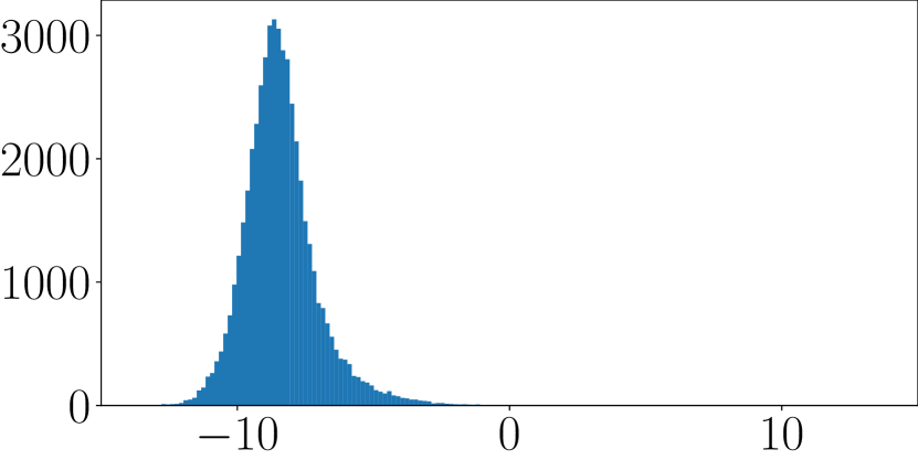
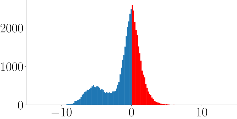
(a) ST

(b) AT

(c) MMA

(d) MART

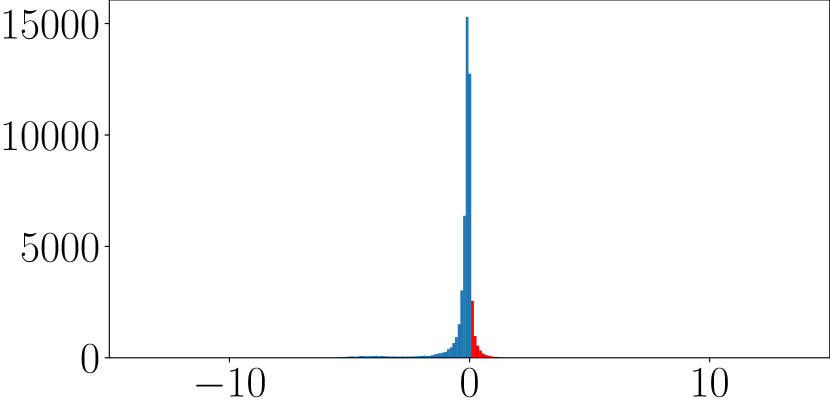
(e) GAIRAT

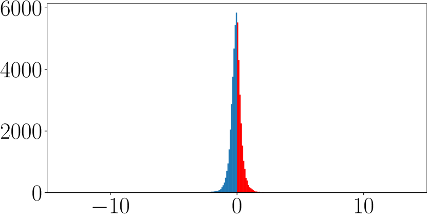
(f) MAIL

Figure 2: Histogram of $\ell_{\mathrm{LM}}$ for training data of CIFAR10 with RN18 at the best (top) and the last (bottom) epoch. Best epoch is the epoch when models achieved the best robust accuracy against PGD by early stopping. ST denotes standard training, i.e., training on clean data. For standard training, we use $\ell_{\mathrm{LM}}$ on clean data $\bm{x}$, while we plot that on adversarial examples $\bm{x}^{\prime}$ for the other methods. Blue bins are the correctly classified data points, and red bins are misclassified samples.

3.2 Histograms of Logit Margin Loss

Since logit margin losses determine the number of potentially misclassified samples, we show the histogram of them for each method on CIFAR10 at the last epoch in Fig. 2. Comparing AT (Fig. 2(b)) with standard training (ST, Fig. 2(a)), AT has two peaks in the histogram. This indicates that the levels of difficulty in increasing the margins in AT are roughly divided into two: difficult samples (right peak) and easy samples (left peak). Difficult samples correspond to the data close to the boundary; i.e., important samples. Next, comparing AT (Fig. 2(b)) with importance-aware methods (Figs. 2(c)-2(f)), their logit margin losses $\ell_{\mathrm{LM}}$ concentrate on zero, and their peaks are sharper than that of AT. This indicates that importance-aware methods fail to increase the logit margins $|\ell_{\mathrm{LM}}|$ for not only important samples but also less-important (easy) samples because the weights for less-important samples are relatively small. Thus, it is necessary to increase the small logit margins for important samples without decreasing those of easy samples. Appendix F.1 provides results under various settings, which show similar tendencies.

4 Proposed Method

In Section 3.2, we observe that (a) training samples are roughly divided into two types via logit margins; difficult and easy (important and less-important) samples, and (b) importance-aware methods reduce the logit margins on less-important samples to focus on important samples. From these observations, our method is based on two ideas: (i) we switch from cross-entropy to an alternative loss for important samples by the criterion of the logit margin loss, and (ii) the alternative loss increases the logit margins of important samples more than weighted cross-entropy.

4.1 One-Vs-the-Rest Loss (OVR)

The logit margin $|z_{k^{*}}(\bm{x})-z_{y}(\bm{x})|$ should be large while keeping Lipschitz constants of logit functions small values. To this end, we need a loss function to penalize small logit margins. The logit margin loss can be an intuitive candidate as such a loss function. However, the logit margin loss only considers the pair of the largest logit $z_{k^{*}}$ and the logit for the true label $z_{y}$, and this is not sufficient for the robustness because $k^{*}$ and $\hat{k}$ in Eq. (3.1) are not necessarily the same. Moreover, the logit margin loss does not have the desirable property for multi-class classification: infinite sample consistent (ISC) (Zhang, 2004; Bartlett et al., 2003; Lin, 2002). To consider the logits for all classes and satisfy ISC, our proposed method uses the one-vs-the-rest loss (OVR):

$$\textstyle\ell_{\mathrm{OVR}}(\bm{z}(\bm{x},\bm{\theta}),y)=\phi(z_{y}(\bm{x}))+\sum_{k\neq y}\phi(-z_{k}(\bm{x})).$$ (7)

When $\phi$ is a differentiable non-negative convex function and satisfies $\phi(z)\!<\!\phi(-z)$ for $z\!>\!0$, OVR satisfies ISC (Zhang, 2004). To satisfy ISC, we set $\phi(z)\!=\!\mathrm{log}(1\!+\!e^{-z})$ and use

$$\textstyle\!\!\ell_{\mathrm{OVR}}(\bm{z}(\bm{x},\bm{\theta}),y) \textstyle\!=\!\mathrm{log}(1\!+\!e^{-z_{y}(\bm{x})})\!\!+\!\!\sum_{k\neq y}\!\mathrm{log}(1\!+\!e^{z_{k}(\bm{x})})$$

$$\textstyle\!=\!-z_{y}(\bm{x})\!+\!\sum_{k}\mathrm{log}(1\!+\!e^{z_{k}(\bm{x})}).$$ (8)

We provide explanation of ISC and the detailed reason for this selection of $\phi(z)$ in Appendix D.

4.2 Behavior of Logit Margin Losses by OVR

To show the effectiveness of OVR in increasing logit margins, we theoretically discuss the difference between OVR and cross-entropy. First, OVR has the following property compared with cross-entropy:

Theorem 4.1.

If we use OVR (Eq. (8)) and softmax as $f_{k}(\bm{x})=e^{z_{k}(\bm{x})}/\sum_{i}e^{z_{i}(\bm{x})}$, we have

$$\textstyle 0\leq\ell_{\mathrm{CE}}(\bm{z}(\bm{x}),y)\leq\ell_{\mathrm{OVR}}(\bm{z}(\bm{x}),y),~{}~{}\forall(\bm{x},y).$$ (9)

When $z_{y}(\bm{x})\!\rightarrow\!+\infty$ and $z_{k}(\bm{x})\!\rightarrow\!-\infty$ for $k\!\neq\!y$, we have $\ell_{\mathrm{OVR}}(\bm{z}(\bm{x}),y)\!\rightarrow\!0$ and $\ell_{\mathrm{CE}}(\bm{z}(\bm{x}),y)\!\rightarrow\!0$.

Thus, OVR is always larger than or equal to cross-entropy, and OVR and cross-entropy approach asymptotically to zero when $|\ell_{\mathrm{LM}}|$ grows to infinity. In fact, we observed that $\ell_{\mathrm{OVR}}(\bm{z},y)$ is about four times greater than $\ell_{\mathrm{CE}}(\bm{z},y)$ for random logits $\bm{z}\!\sim\!\mathcal{N}(\bm{0},\bm{I})$ and randomly selected $y$ from $\{1,\dots,10\}$. Thus, we expect OVR to penalize the small logit margin more strongly than cross-entropy.

Besides this general result, we further investigate the effect of OVR in logit margin losses by using a simple problem. To analyze the behavior of logit margins, we formulate the following problem:

$$\textstyle\min_{\bm{z}}w\ell_{*}(\bm{z},y),$$ (10)

where $\ell_{*}$ is set to $\ell_{\mathrm{OVR}}$ or $\ell_{\mathrm{CE}}$. $\bm{z}\!\in\!\mathbb{R}^{K}$ is a logit vector for a data point $\bm{x}$, and we assume that we can directly move it in this problem. $w\!\in\!\mathbb{R}$ is a weight of the loss, which appears in Eq. (4). To analyze the dynamics of training on Eq. (10), we use the following assumption.

Assumption 4.2.

A logit vector $\bm{z}$ follows the following gradient flow to solve Eq. (10):

$$\textstyle\frac{d\bm{z}}{dt}=-\nabla_{\bm{z}}w\ell_{*}(\bm{z},y),$$ (11)

where $t$ is a time step of training. We assume that $\bm{z}$ is initialized to zeros $\bm{z}=\bm{0}$ at $t=0$.

Equation (11) is a continuous approximation of gradient descent $\bm{z}^{\tau\!+\!1}\!=\!\bm{z}^{\tau}\!\!-\!\eta\nabla_{\bm{z}}\!w\ell_{*}$ and matches it in the limit as $\eta\!\rightarrow\!0$. It is a commonly used method to analyze the training dynamics (Kunin et al., 2021; Elkabetz & Cohen, 2021).

Under Assumption 4.2, we have the following lemmas about the logits in the training of Eq. (10):

Lemma 4.3.

If we use OVR $\ell_{\mathrm{OVR}}(\bm{z},y)$ in Eq. (10), the $k$-th logit $z_{k}(t)$ at time $t$ is

$$\textstyle z_{k}(t)=\begin{cases}\textstyle wt+1-W(e^{wt+1})&~{}~{}k\!=\!y,\\ \textstyle-wt-1-W(e^{wt+1})&~{}~{}k\!\neq\!y,\end{cases}$$ (12)

where $W$ is Lambert $W$ function, which is a function satisfying $x=W(xe^{x})$ (Corless et al., 1996).

Lemma 4.4.

If we use cross-entropy $\ell_{\mathrm{CE}}(\bm{z},y)$ in Eq. (10), the $k$-th logit $z_{k}(t)$ at time $t$ is

$$\textstyle\!\!z_{k}(t)\!=\!\begin{cases}\textstyle\!\frac{Kwt+1}{K}\!-\!\frac{K-1}{K}W(\frac{1}{K-1}e^{\frac{Kwt+1}{K-1}})&\!\!\!k\!=\!y,\\ \textstyle\!-\frac{Kwt+1}{K(K-1)}\!+\!\frac{1}{K}W(\frac{1}{K-1}e^{\frac{Kwt+1}{K-1}})&\!\!\!k\!\neq\!y,.\end{cases}$$ (13)

These lemmas give the trajectories of logit vectors in minimization of OVR and cross-entropy, respectively. Both methods increase the logit for the true labels $z_{y}$ and decrease the others, but their speeds are different. From the above lemmas, we derive the trajectory of the logit margin loss:

Theorem 4.5.

Logit margin losses for the logit vector $\bm{z}^{OVR}$ in the minimization of weighted OVR and logit vector $\bm{z}^{CE}$ in the minimization of weighted cross-entropy at time $t$ are

$$\textstyle\ell_{\mathrm{LM}}(\bm{z}^{OVR}(t)) \textstyle=-2w_{1}t-2+2W(e^{w_{1}t+1}),$$ (14)

$$\textstyle\ell_{\mathrm{LM}}(\bm{z}^{CE}(t)) \textstyle=-\frac{Kw_{2}t+1}{K-1}+W(\frac{1}{K-1}e^{\frac{Kw_{2}t+1}{K-1}}),$$ (15)

where $w_{1}\!\in\!\mathbb{R}$ and $w_{2}\!\in\!\mathbb{R}$ are weights for OVR and cross-entropy, respectively. For large $t$, they are approximated by

$$\textstyle\!\!\!\!\!\ell_{\mathrm{LM}}(\bm{z}^{OVR}(t)) \textstyle\!\approx\!-\log(w_{1}t+1)^{2},$$ (16)

$$\textstyle\!\!\!\!\!\ell_{\mathrm{LM}}(\bm{z}^{CE}(t)) \textstyle\!\approx\!-\log(Kw_{2}t+1\!-\!\log(K\!-\!1)^{K\!-\!1}\!),$$ (17)

and $\lim_{t\rightarrow\infty}\!\frac{\ell_{\mathrm{LM}}(\bm{z}^{OVR})(t)}{\ell_{\mathrm{LM}}(\bm{z}^{CE})(t)}\!=\!2$ for any fixed $w_{1}$, $w_{2}$, and $K$.

This theorem shows the difference in trajectories of logit margin losses between OVR and cross-entropy under Assumption 4.2. Regardless of the values of weights $w_{1}$ and $w_{2}$, cross-entropy does not increase the logit margins as large as OVR for sufficiently large $t$. Thus, OVR increases the small logit margins more effectively than GAIRAT and MAIL, which use weighted cross-entropy (Eq. (4)).

Figure 3(a) plots the trajectory of logit margin losses $\ell_{\mathrm{LM}}$ in the minimization of Eq. (10). This figure shows the solutions in Theorem 4.5 (solid lines): we use Eqs. (14) and (15) unless overflow occurs due to exponential functions and use Eqs. (16) and (17) when it occurs. It also plots numerical solutions of Eq. (11) by using gradients and the Runge–Kutta method as a reference (dashed lines). In Fig. 3(a), Eqs. (14)-(17) exactly match the numerical solutions of RK, and thus, logit margins follow Theorem 4.5. In addition, Fig. 3(a) shows that OVR decreases logit margin losses more than cross-entropy against $t$ regardless of $K$ and $w$. Thus, using OVR is more suitable for increasing the logit margin on important samples than previous weighting approaches like GAIRAT and MAIL. Figure 3(b) plots trajectories of $\ell_{\mathrm{LM}}$ in adversarial training (Eq. (1)) on CIFAR10. It shows that the logit margin $|\ell_{\mathrm{LM}}|$ of OVR is about twice as large as that of cross-entropy at the last epoch ($\frac{\ell_{\mathrm{LM}}(\bm{z}^{OVR})}{\ell_{\mathrm{LM}}(\bm{z}^{CE})}\!=\!1.87$ for $w\!=\!1$), like the case of Theorem 4.5. Thus, problem Eq. (10) is simple but precise enough to explain the difference in the logit margins between OVR and cross-entropy on a real dataset. In fact, $\frac{\ell_{\mathrm{LM}}(\bm{z}^{OVR})}{\ell_{\mathrm{LM}}(\bm{z}^{CE})}$ at the last epoch is in [1.5, 2] on other datasets, including CIFAR100 ($K\!=\!100$) (Appendix F.3).

As above, we prove that OVR is more effective for increasing logit margins of important samples than weighting cross-entropy. In the next section, we compose the objective functions switching between OVR and cross-entropy for important and less-important samples.

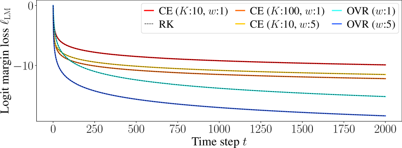
(a) Minimization of Eq. (10)

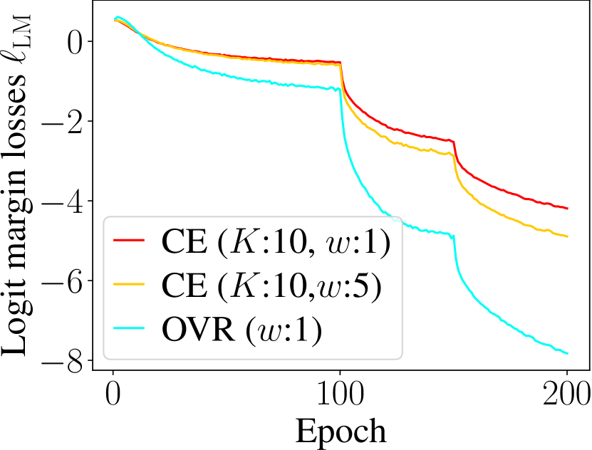
(b) CIFAR 10 (RN18)

Figure 3: Trajectories of $\ell_{\mathrm{LM}}$. CE denotes cross-entropy. In (a), RK denotes 4-th order Runge–Kutta method with the step size of 0.1. (b) is trajectory in adversarial training on CIFAR10, and its setup is provided in Appendix F.3

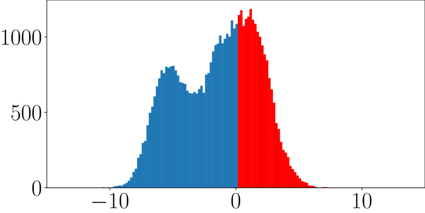
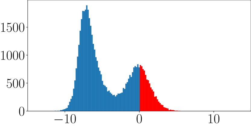
Figure 4: Histogram of $\ell_{\mathrm{LM}}$ of SOVR at the best (top) and the last (bottom) epoch.

4.3 Proposed Objective Function: SOVR

Our proposed objective function is

$$\textstyle\mathcal{L}_{\mathrm{SOVR}}(\bm{\theta})=\frac{1}{N} \textstyle\left[\sum_{(\bm{x},y)\in\mathbb{S}}\ell_{\mathrm{CE}}(\bm{z}(\bm{x}^{\prime},\bm{\theta}),y)\right.$$

$$\textstyle\left.+\lambda\sum_{(\bm{x},y)\in\mathbb{L}}\ell_{\mathrm{OVR}}(\bm{z}(\bm{x}^{\prime},\bm{\theta}),y)\right],$$ (18)

where $\mathbb{S}$ is a set where logit margin losses $\ell_{LM}$ are smaller than those in the set $\mathbb{L}$, and we have $|\mathbb{S}|\!+\!|\mathbb{L}|=N$. These sets correspond to easy and difficult samples in Fig. 2(b). In our method, we select the top $M$ % data points in minibatch of SGD as $\mathbb{L}$. $\lambda$ is a hyperparameter to balance the loss, and $\bm{x}^{\prime}$ is an adversarial example generated by Eq. (2). The proposed algorithm is shown in Appendix B. Since we do not additionally generate the adversarial examples for $\ell_{\mathrm{OVR}}$, the overhead of our method is negligible: $O(b\log\frac{M}{100}b)$ where $b$ is minibatch size. In the same way to Section 3.2, we evaluate the histograms of logit margin losses for SOVR on CIFAR10 in Fig. 4. It shows that SOVR succeeds at increasing the left peak compared with AT (Fig. 2(b)). This is because OVR strongly penalizes important samples in the right peak and moves them into the left peak.

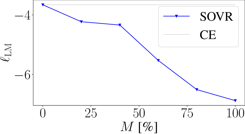
(a) $\ell_{\mathrm{LM}}(\bm{x}^{\prime})$

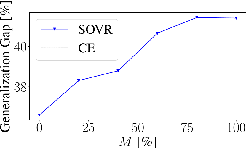
(b)

Generalization Gap

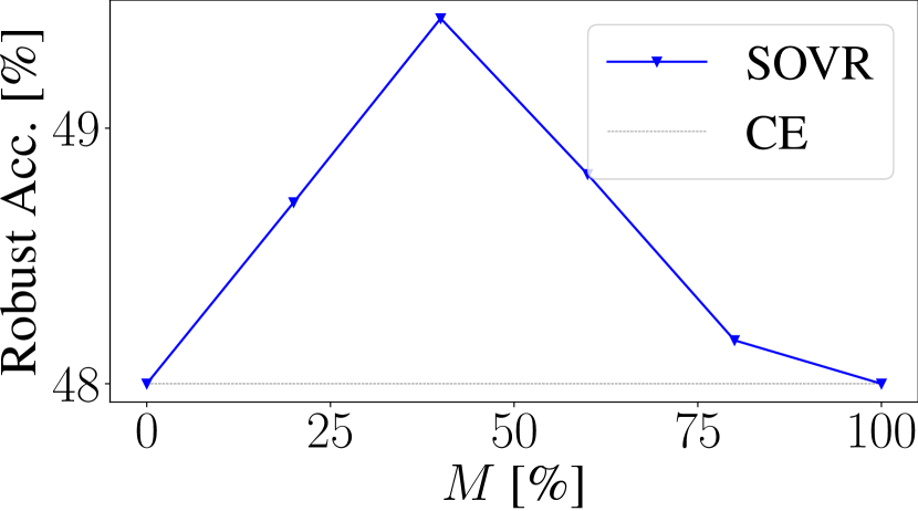
(c)

Robust Acc.

Figure 5: The effect of rate $M$ of applying OVR. $\lambda$ is set to 0.4. $M\!=\!0$ corresponds to the result of AT with cross-entropy. Generalization gap is a gap between training and test robust accuracies against PGD ($\mathcal{K}$=20) at the last epoch. Robust Acc. is robust accuracy against Auto-Attack.

Though OVR increases logit margins as explained in Section 4.2, we found that OVR ($M\!=\!100$) is inferior to SOVR because OVR for less-important samples can cause overfitting. Figure 5 plots the effect of $M$ in terms of $\ell_{\mathrm{LM}}$ at the last epoch, generalization gap at the last epoch, and robust accuracy against Auto-Attack on CIFAR10. It shows that $\ell_{\mathrm{LM}}$ monotonically decreases, i.e., robustness improves, when increasing $M$. However, the generalization gap increases at the same time. Robust accuracy takes the largest value at $M\!=\!40$. Thus, it is necessary to focus on important samples by switching losses, like existing importance-aware methods. We provide the evaluation of effects of $\lambda$ in Appendix F.4, which shows the similar tendencies.

4.4 Extension for Other Defense Methods

Since SOVR only modifies the objective function, it can be used with the optimization algorithms for robustness, e.g., adversarial weight perturbation (AWP) (Wu et al., 2020) or self-ensemble adversarial training (SEAT) (Wang & Wang, 2022), and generative data augmentation (Gowal et al., 2021; Rebuffi et al., 2021), which improve generalization performance in adversarial training. However, SOVR is difficult to use with TRADES (Zhang et al., 2019) because TRADES also modifies the objective function. To combine our method with TRADES, we propose TSOVR, which uses SOVR instead of cross-entropy for clean data:

$$\!\!\!\!\!\textstyle\mathcal{L}_{\mathrm{TS}}\!(\bm{\theta})\!=\!\frac{1}{N}[\mathcal{L}_{\mathrm{SOVR}}\!+\!\beta_{T}\!\sum_{n}\!\mathrm{KL}(\bm{f}(\bm{x}_{n},\!\bm{\theta}),\!\bm{f}(\bm{x}^{\prime}_{n},\!\bm{\theta})\!)]$$ (19)

$$\!\!\!\!\!\textstyle\mathcal{L}_{\mathrm{SOVR}}\!=\!\sum_{(\bm{x},y)\in\mathbb{S}}\ell_{\mathrm{CE}}(\bm{z}(\bm{x},\bm{\theta}),y)$$

$$~{}~{}~{}~{}~{}~{}~{}~{}~{}~{}~{}~{}~{}~{}\textstyle+\lambda\sum_{(\bm{x},y)\in\mathbb{L}}\ell_{\mathrm{OVR}}(\bm{z}(\bm{x},\bm{\theta}),y)$$ (20)

where $\lambda$ and $\beta_{T}$ are hyperparameters. $\bm{x}^{\prime}_{n}$ is obtained by $\bm{x}^{\prime}_{n}=\max_{||\bm{x}^{\prime}_{n}-\bm{x}||_{p}\leq\varepsilon}\!\mathrm{KL}(\bm{f}(\bm{x}_{n},\bm{\theta}),\bm{f}(\bm{x}_{n}^{\prime},\bm{\theta}))$. We evaluate the combinations of SOVR with AWP (Wu et al., 2020), SEAT (Wang & Wang, 2022), and data augmentation using synthetic data (Gowal et al., 2021) in the experiments.

5 Related Work

The difference in importance of data points in adversarial training has been investigated in several studies (Wang et al., 2020a; Zhang et al., 2020; Sanyal et al., 2021; Dong et al., 2022). Zhang et al. (2020) investigated the effect of difficult samples on natural generalization performance, i.e., generalization performance on clean data. They presented FAT that improves the robustness without compromising the natural generalization performance. Unlike FAT, SOVR focuses on the robust performance. Sanyal et al. (2021) and Dong et al. (2022) have investigated the effect of memorization of difficult samples in the generalization performance of adversarial training. Whereas they focused on reducing generalization gap by regularization, our method reduces robust error on test data by reducing training robust error; i.e., mitigating underfitting more than overfitting. Cisse et al. (2017); Tsuzuku et al. (2018); Zhang et al. (2021a) have shown the relation between robustness, logit margins and Lipschitz constants similar to our justification (Section 3). They used them to present certified defense methods. However, their empirical robustness is not as well as that of AT. Though MMA (Ding et al., 2020) is the most well-known method to increase logit margins empirically, our experiment shows that MMA does not necessarily increase logit margins. OVR has been used as the loss function of multi-class classification (Zhang, 2004), but there are few studies using it as a loss function of deep neural networks. Padhy et al. (2020) and Saito & Saenko (2021) used OVR for OOD detection and open-set domain adaptations, respectively. However, they did not discuss the effect of OVR in logit margins, and our study is the first work to reveal the effect of OVR in adversarial robustness and logit margins theoretically and experimentally. Studies of (Hitaj et al., 2021; Croce & Hein, 2020; Kim et al., 2021) have reported the vulnerabilities of some importance-aware methods to logit scaling attacks or Auto-Attack but few studies discuss the causes. Kim et al. (2021) have pointed out that the cause is high entropy in GAIRAT and MART and presented EWAT (entropy-weighted adversarial training), which imposes a higher weight on the higher entropy. However, the logit margin is more related to robustness than entropy as discussed in Section 3. Furthermore, weighted cross-entropy in EWAT is less effective than OVR as shown Theorem 4.5.

6 Experiments

6.1 Setup

We conducted the experiments for evaluating SOVR. We first compare SOVR and TSOVR with Madry’s AT (Madry et al., 2018), MMA (Ding et al., 2020), MART (Wang et al., 2020a), GAIRAT (Zhang et al., 2021b), MAIL (Liu et al., 2021), and EWAT (Kim et al., 2021). Additionally, we evaluated TRADES as another baseline that does not consider the importance of data points. We used three datasets: CIFAR10, SVHN, and CIFAR100 (Krizhevsky & Hinton, 2009; Netzer et al., 2011). Next, we evaluate the combination of SOVR and AWP (Wu et al., 2020), SEAT (Wang & Wang, 2022), and data augmentation using 1M synthetic data by DDPM (1M DDPM) (Rebuffi et al., 2021; Gowal et al., 2021). Our experimental codes are based on source codes provided by (Wu et al., 2020; Wang et al., 2020a; Ding et al., 2020; Rade, 2021), and 1M synthetic data is provided in (Gowal et al., 2021). We used PreActResNet-18 (RN18) (He et al., 2016) for all datasets and WideResNet-34-10 (WRN) (Zagoruyko & Komodakis, 2016) for CIFAR10. We used PGD ($\mathcal{K}\!=\!10$, $\eta\!=\!2/255$, $\varepsilon\!=\!8/255$) in training. We used early stopping by evaluating test robust accuracies against PGD with $\mathcal{K}\!=\!10$. For AWP, SEAT, and 1M DDPM, we use the original public codes (Wu et al., 2020; Wang & Wang, 2022; Rebuffi et al., 2021). For AT+AWP and SOVR+AWP, we use the training setup that is used for TRADES+AWP in Wu et al. (2020) by changing losses because we found that it achieves a better result. We trained models three times and show the average and standard deviation of test accuracies. We set $(M,\lambda)$ in SOVR to $(40,0.4)$ for CIFAR10 (RN18) and SOVR+AWP, $(30,0.4)$ for CIFAR10 (WRN) and $(50,0.6)$ for CIFAR100, $(20,0.2)$ for SVHN, $(40,0.2)$ for SOVR+1M DDPM. We set $(M,\lambda)$ in TSOVR to $(80,0.8)$ for CIFAR10 (RN18), $(20,0.8)$ for CIFAR10 (WRN) and SVHN, $(50,0.5)$ for CIFAR100, $(100,1.2)$ for TSOVR+AWP, and $(100,1.6)$ for SOVR+1M DDPM. We use Auto-Attack to evaluate the robust accuracy on test data. In Appendix E and F, we provide the details of setups and additional results, e.g., evaluation using other various attacks. To determine the statistical significant difference, we use t-test with p-value of 0.05.

6.2 Results

Table 1: Robust accuracy against Auto-Attack and clean accuracy on test datasets.

Robust Accuracy against Auto-Attack ($L_{\infty}$, $\varepsilon\!=\!8/255$)
	AT	MART	MMA	GAIRAT	MAIL	EWAT	SOVR	TRADES	TSOVR
CIFAR10 (RN18)	48.0$\pm$0.2	46.9$\pm$0.3	37.2$\pm$0.9	37.7$\pm$ 1	39.6$\pm$0.4	48.2$\pm$0.7	$49.4\pm 0.3$	48.8$\pm$ 0.3	$\bm{49.8\pm 0.1}$
CIFAR10 (WRN)	51.9$\pm$0.5	50.44$\pm$0.09	43.1$\pm$1	41.8$\pm$0.6	43.3$\pm$0.1	51.6$\pm$0.3	$53.1\pm 0.2$	52.9$\pm$ 0.3	$\bm{53.3\pm 0.1}$
SVHN (RN18)	45.6$\pm$0.4	46.9$\pm$0.3	41.0$\pm$1	37.6$\pm$0.6	41.2$\pm$0.3	47.6$\pm$0.4	$48.5\pm 0.4$	49.4$\pm$ 0.3	$\bm{49.87\pm 0.02}$
CIFAR100 (RN18)	23.7$\pm$0.3	23.9$\pm$0.1	18.4$\pm$0.2	19.8$\pm$0.5	16.7$\pm$0.3	23.52$\pm$0.06	$24.3\pm 0.2$	23.2$\pm$ 0.1	$\bm{24.61\pm 0.07}$
Clean Accuracy
CIFAR10 (RN18)	81.6$\pm$0.5	78.3$\pm$1	$\bm{85.5\pm 0.7}$	78.7$\pm$ 0.7	79.5$\pm$0.4	82.8$\pm$0.4	81.9$\pm$0.2	82.5$\pm$0.2	81.4$\pm$0.2
CIFAR10 (WRN)	85.6$\pm$0.1	81.5$\pm$1	$\bm{87.8\pm 1}$	83.0$\pm$0.7	82.2$\pm$0.4	86.0$\pm$0.5	85.0$\pm$0.2	84.2$\pm$0.7	83.1$\pm$0.2
SVHN (RN18)	89.8$\pm$0.6	86.9$\pm$0.6	$\bm{93.9\pm 0.4}$	89.9$\pm$0.4	89.4$\pm$0.4	90.2$\pm$0.6	90.0$\pm$1	88.7$\pm$1	88.5$\pm$0.5
CIFAR100 (RN18)	53.0$\pm$0.7	49.2$\pm$0.1	$\bm{60.6\pm 0.6}$	52.0$\pm$0.5	46.5$\pm$0.5	54.2$\pm$1	52.1$\pm$0.8	53.8$\pm$0.2	51.6$\pm$0.2

Table 2: Robust accuracy against Auto-Attack ($L_{\infty}$, $\varepsilon=8/255$) on test dataset of CIFAR10. SEAT uses WideResNet32-10 following Wang & Wang (2022), and 1M DDPM uses WideResNet28-10 following Gowal et al. (2021); Rebuffi et al. (2021)

	AWP (WRN34-10)				SEAT		+1M DDPM Gowal et al. (2021); Rebuffi et al. (2021)
	AT+AWP	SOVR+AWP	TRADES+AWP	TSOVR+AWP	SEAT	+SOVR	AT	TRADES	SOVR	TSOVR
Robust Acc.	55.0$\pm$0.2	56.03$\pm$0.07	55.6$\pm$0.4	56.4$\pm$0.2	54.9$\pm$0.1	55.5$\pm$0.3	59.3$\pm$0.9	60.13$\pm$0.5	60.9$\pm$0.1	60.9$\pm$0.2
Clean Acc.	87.8$\pm$0.1	86.9$\pm$0.4	84.9$\pm$0.5	84.9$\pm$0.4	86.8$\pm$0.4	86.5$\pm$0.1	88.46$\pm$0.05	86.1$\pm$0.4	88.05$\pm$0.08	86.08$\pm$0.07

We list the robust accuracy against Auto-Attack on all datasets in Tab. 1. Comparing SOVR with importance-aware methods and AT, SOVR outperforms them in terms of the robustness against Auto-Attack and the difference is statistically significant. This is because SOVR increases the logit margins $|\ell_{\mathrm{LM}}|$ by using OVR. In fact, Fig. 4 shows that SOVR increases the logit margins $|\ell_{\mathrm{LM}}|$ for important samples. MART improved robustness on SVHN and CIFAR100. This might be because MART does not just impose weights on the loss. However, its improvement is less than SOVR. EWAT also achieves higher robust accuracies than AT on several datasets in Tab. 1. However, EWAT is not as robust as SOVR because EWAT employs weighted cross-entropy, which is less effective at increasing logit margins than OVR (Theorem 4.5). In Tab. 1, SOVR slightly sacrifices clean accuracies under some settings. We provide the histograms of logit margin losses on all datasets in Appendix F.1, which also show SOVR increases margins. Comparing SOVR with TRADES and TSOVR, SOVR achieves comparable robust accuracy to TRADES, and TSOVR achieves the best robust accuracy. In addition, SOVR achieves the largest value of robust accuracy + clean accuracy in almost all settings, which is discussed in Section 6.2.3.

6.2.1 Empirical Evaluation of Potentially Misclassified Samples

As discussed in Section 3.1, we can evaluate the robustness near each data point via logit margins and Lipschitz constants of the class-wise logit functions. In this section, we estimate the number of potentially misclassified samples for each method. Since Lipschitz constants for deep neural networks are difficult to compute due to the complexity, we compute the gradient norm of the logit function instead of Lipschitz constants. This is because the gradient norm satisfies $\sup_{\bm{x}}||\nabla_{\bm{x}}z_{k}(\bm{x})||_{1}\!=\!L_{k}$ for $L_{k}$ such as $|z_{k}(\bm{x}_{1})\!-\!z_{k}(\bm{x}_{2})|\!\leq\!L_{k}||\bm{x}_{1}\!-\!\bm{x}_{2}||_{\infty}$ (Jordan & Dimakis, 2020), and we have

Proposition 6.1.

If a data point $\bm{x}$ satisfies

$$\textstyle z_{k^{*}}\!(\bm{x})\!-\!z_{y}(\bm{x})\!>\!-(\max_{k}||\nabla_{\bm{x}}z_{k}(\bm{x})||_{1}\!+\!||\nabla_{\bm{x}}z_{y}(\bm{x})||_{1})\varepsilon,$$ (21)

it is a potentially misclassified sample.

Thus, we can empirically estimate the number of potentially misclassified samples on each method by the gradient norms. Figure 6 plots the rate of data points that satisfy Eq. (21), which are potentially misclassified samples. Comparing Fig. 6 with Tab. 1, when the methods have the large rate on test data, they have low robust accuracies against Auto-Attack. This indicates that this rate is a reasonable metric for estimating robustness though it uses gradient norms instead of Lipschitz constants. Whereas most importance-aware methods have higher rates than AT due to small logit margins, SOVR has lower rate. This is because SOVR increases logit margins without increasing gradient norms by using OVR, which is more effective in increasing logit margins than weighted cross-entropy (Section 4.2). In Fig. 6, EWAT does not necessarily increase the rate because EWAT uses weighted cross-entropy. We discuss the reason the rate of AT gets close to SOVR on CIFAR100 in Appendix F.9.

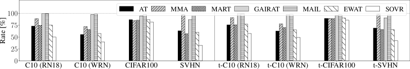
Figure 6: Rate of data satisfying Eq. (21). C10 and t- represent CIFAR10 and test data, respectively.

6.2.2 Extension for Other Methods

To improve the robust accuracy on test data, our method mostly focuses on improving the robustness around training data points rather than regularization. Even so, SOVR can be used with recent regularization methods (Wu et al., 2020; Wang & Wang, 2022) and data augmentation (Rebuffi et al., 2021; Gowal et al., 2021). We evaluated the combination of SOVR and AWP, SOVR and SEAT, and SOVR and data augmentation using 1M synthetic data by DDPM (1M DDPM). Table 2 lists the robust accuracy of the combinations against Auto-Attack and shows that SOVR improved the performance of other recent methods. Thus, SOVR and these methods complementarily improve the performance.

6.2.3 Evaluation of Trade-off

We evaluate the trade-off between robustness and clean accuracy. Figure 7 plots clean accuracy and robust accuracy against Auto-Attack when using WRN on CIFAR10. Diagonal lines are lines satisfying $\mathrm{CleanAcc.}\!+\!\mathrm{RobustAcc.}\!=\!\mathrm{Const}$ through SOVR, SOVR+AWP, SOVR+SEAT, and SOVR+1M DDPM. SOVR achieves a good trade-off: Robust Acc. + Clean Acc. of SOVR, SOVR+AWP, and SOVR+DDPM are the best values under each condition. If we require the most robust models with sacrificing clean accuracies, TSOVR achieves the best robust accuracy against Auto-Attack. Therefore, SOVR and TSOVR are better objective functions than TRADES and cross-entropy in terms of trade-off and robustness, respectively.

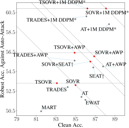
Figure 7: Trade-off between clean and robust accuracies (WRN). $*$ use WRN28-10 and $\dagger$ use WRN32-10.

7 Conclusion

We investigated the reason importance-aware methods fail to improve the robustness against Auto-Attack. Our empirical results showed the reason to be that they decrease logit margins of less-important samples besides those of important samples. From the observation, we proposed SOVR, which switches from cross-entropy to OVR in order to focus on important samples. We proved that OVR increases logit margins more than cross-entropy for a simple problem and experimentally showed that SOVR increases the margins of important samples and improves the robustness.

Appendix A Proofs

A.1 Proof of Proposition 3.2

Proof.

From the definition of Lipschitz constants, we have

$$|z_{k}(\bm{x}+\bm{\delta})-z_{k}(\bm{x})|\leq L_{k}||\bm{x}+\bm{\delta}-\bm{x}||_{\infty}=L_{k}\varepsilon,$$ (22)

Thus, we have $z_{k}(\bm{x}+\bm{\delta})\leq z_{k}(\bm{x})+L_{k}\varepsilon$ if $z_{k}(\bm{x}+\bm{\delta})\geq z_{k}(\bm{x})$ and $z_{k}(\bm{x}+\bm{\delta})\geq z_{k}(\bm{x})-L_{k}\varepsilon$ if $z_{k}(\bm{x}+\bm{\delta})\leq z_{k}(\bm{x})$. Therefore, the following inequalities hold for the not potentially misclassified samples:

$$\max_{k\neq y}z_{k}(\bm{x}+\bm{\delta})-z_{y}(\bm{x}+\bm{\delta}) \leq z_{k^{\prime}}(\bm{x})+L_{k^{\prime}}\varepsilon-(z_{y}(\bm{x})-L_{y}\varepsilon)$$

$$\leq z_{k^{*}}(\bm{x})+L_{\hat{k}}\varepsilon-z_{y}(\bm{x})+L_{y}\varepsilon$$

$$\leq z_{k^{*}}(\bm{x})-z_{y}(\bm{x})+(L_{\hat{k}}+L_{y})\varepsilon,$$ (23)

where $k^{\prime}\!=\!\mathrm{arg}\max_{k\neq y}z_{k}(\bm{x}+\bm{\delta})$, $k^{*}\!=\!\mathrm{arg}\max_{k\neq y}z_{k}(\bm{x})$, and $\hat{k}\!=\!\mathrm{arg}\max_{k}L_{k}$. From $z_{k^{*}}(\bm{x})-z_{y}(\bm{x})\leq-(L_{\hat{k}}+L_{y})\varepsilon$ for not potentially misclassified samples and Eq. (23), we have $\max_{k\neq y}z_{k}(\bm{x}+\bm{\delta})-z_{y}(\bm{x}+\bm{\delta})\leq 0,~{}~{}\forall\bm{\delta}\in\{||\bm{\delta}||_{\infty}\leq\varepsilon\}$. Thus, models are guaranteed to classify adversarial examples of these data points accurately. ∎

A.2 Proof of Theorem 4.1

Proof.

By using logit functions, $\ell_{\mathrm{CE}}$ can be written as

$$\textstyle\ell_{\mathrm{CE}}(\bm{z}(\bm{x},\bm{\theta}),y)=-z_{y}(\bm{x})+\mathrm{log}\sum_{k}e^{z_{k}(\bm{x})}.$$ (24)

when a model uses a softmax function. Compared with OVR $\ell_{\mathrm{OVR}}(\bm{z}(\bm{x},\bm{\theta}),y)\textstyle=-z_{y}(\bm{x})+\sum_{k}\mathrm{log}(1+e^{z_{k}(\bm{x})})$, the difference is only the second term. Thus, $\ell_{\mathrm{OVR}}(\bm{z}(\bm{x},\bm{\theta}),y)-\ell_{\mathrm{CE}}(\bm{z}(\bm{x},\bm{\theta}),y)$ can be written as

$$\textstyle\ell_{\mathrm{OVR}}(\bm{z}(\bm{x},\bm{\theta}),y)-\ell_{\mathrm{CE}}(\bm{z}(\bm{x},\bm{\theta}),y) \textstyle=\sum_{k}\mathrm{log}(1+e^{z_{k}})-\mathrm{log}\sum_{k}e^{z_{k}},$$ (25)

$$\textstyle=\mathrm{log}\prod_{k}(1+e^{z_{k}})-\mathrm{log}\sum_{k}e^{z_{k}}.$$ (26)

Since a logarithm is a strictly increasing function, we have

$$\textstyle\prod_{k}(1+e^{z_{k}})-\sum_{k}e^{z_{k}}\geq 0\Rightarrow\mathrm{log}\prod_{k}(1+e^{z_{k}})-\mathrm{log}\sum_{k}e^{z_{k}}\geq 0.$$ (27)

Since $e^{z_{k}}\geq 0$ for any $z_{k}\in\mathbb{R}$, we have

$$\textstyle\prod_{k}(1+e^{z_{k}})-\sum_{k}e^{z_{k}}=1+\sum_{k}e^{z_{k}}+R(e^{z_{k}})-\sum_{k}e^{z_{k}}=1+R(e^{z_{k}})\geq 0$$ (28)

where $R(e^{z_{k}})$ is the second or higher order terms of $e^{z_{k}}$, and it takes a positive value because $e^{z_{k}}\!\geq\!0$. Thus, the left hand side of Eq. (27) holds, and we have $\mathrm{log}\prod_{k}(1+e^{z_{k}})-\mathrm{log}\sum_{k}e^{z_{k}}\geq 0$. Therefore, we have $\ell_{\mathrm{OVR}}(\bm{z}(\bm{x},\bm{\theta}),y)-\ell_{\mathrm{CE}}(\bm{z}(\bm{x},\bm{\theta}),y)\geq 0$: i.e., $0\leq\ell_{\mathrm{CE}}(\bm{z}(\bm{x},\bm{\theta}),y)\leq\ell_{\mathrm{OVR}}(\bm{z}(\bm{x},\bm{\theta}),y)$ since $\ell_{\mathrm{CE}}(\bm{z}(\bm{x},\bm{\theta}),y)\geq 0$. Next, when $z_{k}(\bm{x})\rightarrow-\infty$ for $k\neq y$, we have $e^{z_{k}}\rightarrow 0$ and

$$\lim_{\begin{subarray}{c}z_{y}\rightarrow+\infty,\\ z_{k}\rightarrow-\infty~{}\mathrm{for}~{}k\neq y\end{subarray}}\!\!\!\!\!\!\ell_{\mathrm{CE}}(\bm{z}(\bm{x},\bm{\theta}),y)=\lim_{\begin{subarray}{c}z_{y}\rightarrow+\infty,\\ z_{k}\rightarrow-\infty~{}\mathrm{for}~{}k\neq y\end{subarray}}\!\!\!\!\!\!-z_{y}(\bm{x})+\mathrm{log}\sum_{k}e^{z_{k}(\bm{x})}=-z_{y}+\mathrm{log}(e^{z_{y}})=0.$$ (29)

On the other hand, when $z_{y}(\bm{x})\rightarrow+\infty$ and $z_{k}(\bm{x})\rightarrow-\infty$ for $k\neq y$, we have $\mathrm{log}(1+e^{z_{y}})\rightarrow z_{y}$ and $\mathrm{log}(1+e^{z_{k}})\rightarrow 0$. Thus, we have

$$\lim_{\begin{subarray}{c}z_{y}\rightarrow+\infty,\\ z_{k}\rightarrow-\infty~{}\mathrm{for}~{}k\neq y\end{subarray}}\!\!\!\!\!\!\ell_{\mathrm{OVR}}(\bm{z}(\bm{x},\bm{\theta}),y)=\lim_{\begin{subarray}{c}z_{y}\rightarrow+\infty,\\ z_{k}\rightarrow-\infty~{}\mathrm{for}~{}k\neq y\end{subarray}}\!\!\!\!\!\!-z_{y}(\bm{x})+\sum_{k}\mathrm{log}(1+e^{z_{k}(\bm{x})})=-z_{y}+z_{y}=0,$$ (30)

which completes the proof. ∎

A.3 Proof of Lemma 4.3

Proof.

From the assumption, we consider the following ordinary differential equation (ODE):

$$\frac{dz_{k}}{dt}=-\frac{\partial w\ell_{OVR}(\bm{z},y)}{\partial z_{k}}.$$ (31)

The initial condition is $\bm{z}(0)=\bm{0}$. For the correct label $y$, the gradient of OVR is given by

$$\frac{\partial\ell_{OVR}(\bm{z},y)}{\partial z_{y}}=-1+\frac{e^{z_{y}}}{e^{z_{y}}+1}.$$ (32)

Thus, ODE becomes

$$\frac{dz_{y}}{dt} =w(1-\frac{e^{z_{y}}}{e^{z_{y}}+1})$$ (33)

$$(1+e^{z_{y}})d{z_{y}} =wdt$$ (34)

$$z_{y}+e^{z_{y}} =wt+c$$ (35)

$$e^{z_{y}+e^{z_{y}}} =e^{wt+c},$$ (36)

where $c$ is a constant, which is determined by the initial condition. We apply the Lambert $W$ function (Corless et al., 1996) for both sides and use $\log W(x)=\log x-W(x)$ for $x>0$ as

$$e^{z_{y}} =W(e^{wt+c}),$$ (37)

$$z_{y} =wt+c-W(e^{wt+c}).$$ (38)

From the assumption, we have $z_{y}(0)=0$, and thus, $c$ satisfies the following equality:

$$c-W(e^{c})=0.$$ (39)

From $W(xe^{x})=x$, we have $c=1$ and the logit of the correct label is given by

$$z_{y} =wt+1-W(e^{wt+1}).$$ (40)

Next, we consider the logit of another label $z_{k}$ for $k\neq y$. Since the gradient for the logit of incorrect label is $\frac{\partial\ell_{OVR}(\bm{z},y)}{\partial z_{k}}=\frac{e^{z_{k}}}{e^{z_{k}}+1}$, we have

$$\frac{dz_{k}}{dt} =-\frac{we^{z_{k}}}{1+e^{z_{k}}}$$ (41)

$$(e^{-z_{k}}+1)dz_{k} =-wdt.$$ (42)

It is solved in the same way as $z_{y}$, and we have

$$z_{k} =-wt-1+W(e^{wt+1}),$$ (43)

for $k\neq y$, which completes the proof. ∎

A.4 Proof of Lemma 4.4

Proof.

We first solve the ODE for the logit of the correct label $z_{y}$. The gradient of cross-entropy is

$$\frac{\partial\ell_{CE}(\bm{z},y)}{\partial z_{k}}=-\delta_{ky}+\frac{e^{z_{k}}}{\sum_{m}e^{z_{m}}}.$$ (44)

From Eq. (44), we have the following ODE:

$$\frac{dz_{y}}{dt} =w\frac{\sum_{m\neq y}e^{z_{m}}}{\sum_{m\neq y}e^{z_{m}}+e^{z_{y}}}.$$ (45)

Since $\bm{z}=\bm{0}$ at $t=0$, we have $z_{i}=z_{j}$ for $\forall i,j\neq y$. In addition, we have $\sum_{i}\frac{dz_{i}(t)}{dt}=\sum_{i}\frac{w\partial\ell_{CE}(\bm{z},y)}{\partial z_{i}}=0$ for $\forall t$. Thus, logits satisfy the following equality:

$$z_{y} =-(K-1)z_{k},$$ (46)

for $k\neq y$. From Eq. (46), Eq. (45) becomes

$$\frac{dz_{y}}{dt} =w\frac{(K-1)e^{-\frac{1}{K-1}z_{y}}}{(K-1)e^{-\frac{1}{K-1}z_{y}}+e^{z_{y}}}$$ (47)

$$(K-1+e^{\frac{K}{K-1}z_{y}})dz_{y} =w(K-1)dt$$ (48)

$$\frac{K}{K-1}z_{y}+\frac{1}{K-1}e^{\frac{K}{K-1}z_{y}} =\frac{K}{K-1}wt+c$$ (49)

$$\frac{1}{K-1}e^{\frac{K}{K-1}z_{y}}e^{\frac{1}{K-1}e^{\frac{K}{K-1}z_{y}}} =\frac{1}{K-1}e^{\frac{K}{K-1}wt+c}$$ (50)

$$\frac{1}{K-1}e^{\frac{K}{K-1}z_{y}} =W(\frac{1}{K-1}e^{\frac{K}{K-1}wt+c})$$ (51)

$$\frac{K}{K-1}z_{y} =\log\left\{(K-1)W(\frac{1}{K-1}e^{\frac{K}{K-1}wt+c})\right\}$$ (52)

$$z_{y} =wt+\frac{K-1}{K}c-\frac{K-1}{K}W(\frac{1}{K-1}e^{\frac{K}{K-1}wt+c})$$ (53)

where $c$ is a constant, which is determined by the initial condition. From Assumption, we have

$$z_{y}(0) =\frac{K-1}{K}c-\frac{K-1}{K}W(\frac{1}{K-1}e^{c})=0$$ (54)

$$W(\frac{1}{K-1}e^{c}) =c.$$ (55)

Thus, we have $c=\frac{1}{K-1}$ since $W(xe^{x})=x$. From Eqs. (46) and (53), we have

$$z_{y}(t) =wt+\frac{1}{K}-\frac{K-1}{K}W(\frac{1}{K-1}e^{\frac{K}{K-1}wt+\frac{1}{K-1}})$$ (56)

$$z_{k}(t) =-\frac{1}{K-1}wt-\frac{1}{K(K-1)}+\frac{1}{K}W(\frac{1}{K-1}e^{\frac{K}{K-1}wt+\frac{1}{K-1}})~{}~{}\mathrm{for}~{}~{}~{}k\neq y$$ (57)

which completes the proof. ∎

A.5 Proof of Theorem 4.5

From Lemmas 4.3 and 4.4, we have

$$\ell_{\mathrm{LM}}(\bm{z}^{OVR}(t)) =-2w_{1}t-2+2W(e^{w_{1}t+c}),$$ (58)

$$\ell_{\mathrm{LM}}(\bm{z}^{CE}(t)) =-\frac{K}{K-1}w_{2}t-\frac{1}{K-1}+W(\frac{1}{K-1}e^{\frac{K}{K-1}w_{2}t+\frac{1}{K-1}}).$$ (59)

Since $W(x)=\log(x)-\log(\log(x))+O(1)$ for large $x$ (Hoorfar & Hassani, 2007), we have

$$\ell_{\mathrm{LM}}(\bm{z}^{OVR}(t))\approx -2w_{1}t-2+2(w_{1}t+1-\log(w_{1}t+1))$$ (60)

$$= -\log(w_{1}t+1)^{2}$$ (61)

$$\ell_{\mathrm{LM}}(\bm{z}^{CE}(t))\approx -\frac{K}{K-1}w_{2}t-\frac{1}{K-1}$$ (62)

$$-\log(K-1)+\frac{K}{K-1}w_{2}t+\frac{1}{K-1}$$ (63)

$$-\log(-\log(K-1)+\frac{K}{K-1}w_{2}t+\frac{1}{K-1})$$ (64)

$$= -\log(Kw_{2}t+1-(K-1)\log(K-1)).$$ (65)

From the above, we have

$$\lim_{t\rightarrow\infty}\frac{\ell_{\mathrm{LM}}(\bm{z}^{OVR})(t)}{\ell_{\mathrm{LM}}(\bm{z}^{CE})(t)} =\lim_{t\rightarrow\infty}\frac{\log(w_{1}t+1)^{2}+O(1)}{\log(Kw_{2}t+1-(K-1)\log(K-1))+O(1)},$$ (66)

$$=\lim_{t\rightarrow\infty}\frac{2\log t+2\log(w_{1}+t^{-1})+O(1)}{\log t+\log(Kw_{2}+t^{-1}(1-(K-1)\log(K-1)))+O(1)},$$ (67)

$$=\lim_{t\rightarrow\infty}\frac{2+\frac{2}{\log t}\log(w_{1}+t^{-1})+\frac{O(1)}{\log t}}{1+\frac{\log(Kw_{2}+t^{-1}(1-(K-1)\log(K-1)))}{\log t}+\frac{O(1)}{\log t}},$$ (68)

$$=2,$$ (69)

which completes the proof.

A.6 Proof of Proposition 6.1

Proof.

Since we have $\sup_{\bm{x}}||\nabla_{\bm{x}}z_{k}(\bm{x})||_{q}=L_{k}$ for an $L_{k}$-Lipschitz function such as $|z_{k}(\bm{x}_{1})-z_{k}(\bm{x}_{2})|\leq L_{k}||\bm{x}_{1}-\bm{x}_{2}||_{p}$ where $1/q+1/p=1$ (Jordan & Dimakis, 2020), the following inequality holds if $\bm{z}_{k^{*}}(\bm{x})-\bm{z}_{y}(\bm{x})>-(\max_{k}||\nabla_{\bm{x}}z_{k}(\bm{x})||_{1}+||\nabla_{\bm{x}}z_{y}(\bm{x})||_{1})\varepsilon$ and $p=\infty$:

$$\bm{z}_{k^{*}}(\bm{x})-\bm{z}_{y}(\bm{x}) >-(\max_{k}||\nabla_{\bm{x}}z_{k}(\bm{x})||_{1}+||\nabla_{\bm{x}}z_{y}(\bm{x})||_{1})\varepsilon$$

$$\geq-(\max_{k}\sup_{x}||\nabla_{\bm{x}}z_{k}(\bm{x})||_{1}+\sup_{x}||\nabla_{\bm{x}}z_{y}(\bm{x})||_{1})\varepsilon\geq-(L_{\hat{k}}+L_{y})\varepsilon,$$ (70)

because $||\nabla_{\bm{x}}z_{k}(\bm{x})||_{1}\leq L_{k}$ for $p=\infty$. Thus, we have $z_{k^{*}}(\bm{x})-z_{y}(\bm{x})>-(L_{\hat{k}}+L_{y})\varepsilon$ on this condition, which completes the proof. ∎

Appendix B Algorithm

The proposed algorithm is shown in Algorithm 1. We first generate $\bm{x}^{\prime}$ in Line 3 and compute the $\ell_{LM}$ for them in Line 4. In Line 6, we select the top $M$ % samples in minibatch and add them to $\mathbb{L}$. Finally, we compute the objective $\mathcal{L}_{\mathrm{SOVR}}$ and its gradient to update $\bm{\theta}$. Since we do not additionally generate the adversarial examples for $\ell_{\mathrm{OVR}}$, the overhead of our method is $O(|\mathbb{B}|\log\frac{M}{100}|\mathbb{B}|)$, which is the computation cost of the heap sort for selecting $\mathbb{L}$ in Line 6. It is negligible in the whole computation since deep models have huge parameter-size compared with batch-size $|\mathbb{B}|$.

Algorithm 1 Switching one-vs-the-rest by the criterion of a logit margin loss

1:  Select the minibatch $\mathbb{B}$

2:  for $\bm{x}_{n}\in\mathbb{B}$ do

3:     Generate adversarial examples $\bm{x}_{n}^{\prime}=\mathrm{arg}\!\max_{||\bm{x}_{n}^{\prime}-\bm{x}_{n}||_{\infty}\leq\varepsilon}\ell_{\mathrm{CE}}(\bm{z}(\bm{x}_{n}^{\prime},\bm{\theta}),y_{n})$ by PGD

4:     $\ell_{\mathrm{LM}}(\bm{z}(\bm{x}_{n}^{\prime},\bm{\theta}),y_{n})=\max_{k\neq y_{n}}z_{k}(\bm{x}_{n}^{\prime})-z_{y_{n}}(\bm{x}_{n}^{\prime})$

5:  end for

6:  Select top $\frac{M}{100}|\mathbb{B}|$ samples of $(\bm{x}_{n}^{\prime},y_{n})$ in terms of $\ell_{\mathrm{LM}}(\bm{z}(\bm{x}_{n}^{\prime},\bm{\theta}),y_{n})$ and add them to $\mathbb{L}$

7:  $\mathcal{L}_{\mathrm{SOVR}}(\bm{\theta})=\frac{1}{|\mathbb{B}|}\left[\sum_{(\bm{x},y)\in\mathbb{B}\backslash\mathbb{L}}\ell_{\mathrm{CE}}(\bm{z}(\bm{x}^{\prime},\bm{\theta}),y)+\lambda\sum_{(\bm{x},y)\in\mathbb{L}}\ell_{\mathrm{OVR}}(\bm{z}(\bm{x}^{\prime},\bm{\theta}),y)\right]$

8:  Update the parameter $\bm{\theta}\leftarrow\bm{\theta}-\eta\nabla_{\bm{\theta}}\mathcal{L}_{\mathrm{SOVR}}(\bm{\theta})$

Appendix C Additional Explanation about Previous Methods

C.1 MART (Wang et al., 2020a)

MART (Wang et al., 2020a) uses a similar approach to importance-aware methods. It regards misclassified samples as important samples and minimizes

$$\textstyle\ell_{\mathrm{MART}}(\bm{x}^{\prime},y,\bm{\theta}) \textstyle=\mathrm{BCE}(\bm{f}(\bm{x}^{\prime},\bm{\theta}),y)+\lambda\mathrm{KL}(\bm{f}(\bm{x},\bm{\theta}),\bm{f}(\bm{x}^{\prime},\bm{\theta}))\cdot(1-f_{y}(\bm{x},\bm{\theta})),\textstyle$$ (71)

where $\mathrm{BCE}(\bm{f}(\bm{x}^{\prime},\bm{\theta}),y)\!=\!-\mathrm{log}(f_{y}(\bm{x}^{\prime},\bm{\theta}))\!-\!\mathrm{log}(1\!-\!\max_{k\neq y}f_{k}(\bm{x}^{\prime},\bm{\theta}))$ and $\mathrm{KL}$ is Kullback-Leibler divergence. MART controls the difference between the loss on less-important and important samples via $1-f_{y}(\bm{x}_{n},\bm{\theta})$: MART tends to ignore the second term when the model is confident in the true label.

C.2 MMA (Ding et al., 2020)

MMA (Ding et al., 2020) attempts to maximize the distance between data points and the decision boundary for robustness. MMA regards $\min_{\bm{\delta}}||\bm{\delta}_{n}||_{\infty}$ subject to $\{\ell_{\mathrm{LM}}(\bm{z}(\bm{x}+\bm{\delta},\bm{\theta}),y)\geq 0\}$ as the distance. By using this distance, MMA minimizes the following loss:

$$\textstyle\mathcal{L}(\bm{\theta})\textstyle=\frac{1}{3}\sum_{n=1}^{N}\ell_{\mathrm{CE}}(\bm{z}(\bm{x}_{n},\bm{\theta}),y_{n})+\frac{2}{3}\mathcal{L}_{\mathrm{MMA}}(\bm{\theta})$$ (72)

$$\textstyle\mathcal{L}_{\mathrm{MMA}}(\bm{\theta})\textstyle\!=\!\sum_{(\bm{x},y)\in\mathcal{S^{+}}\cap\mathcal{H}}\ell_{\mathrm{CE}}(\bm{z}(\bm{x}\!+\!\bm{\delta}_{\mathrm{MMA}},\bm{\theta}),y)\!+\!\sum_{(x,y)\in\mathcal{S^{-}}}\ell_{\mathrm{CE}}(\bm{z}(\bm{x},\bm{\theta}),y)$$ (73)

$$\textstyle\bm{\delta}_{\mathrm{MMA}}\textstyle=\mathrm{arg}\min_{\ell_{\mathrm{SLM}}(\bm{z}(\bm{x}+\bm{\delta},\bm{\theta}),y)\geq 0}||\bm{\delta}||_{\infty}$$ (74)

$$\textstyle\ell_{\mathrm{SLM}}(\bm{z}(\bm{x},\bm{\theta}),y)\textstyle=\mathrm{log}\sum_{k\neq y}e^{z_{k}(\bm{x})}-z_{y}(x)$$ (75)

where $\mathcal{S^{+}}$ is a set of correctly classified data points, and $\mathcal{S^{-}}$ is a set of misclassified samples. $\mathcal{H}$ is a set of data points that have a smaller distance than threshold $d_{\mathrm{max}}$ as $\mathcal{H}=\{(x_{n},y_{n})|\min_{\bm{\delta}_{n}}||\bm{\delta}_{n}||_{\infty}\leq d_{\mathrm{max}}\}$. Since MMA uses $\bm{\delta}$ whose magnitude $||\bm{\delta}||_{\infty}$ depends on data points as Eq. (74), we consider that it has similar effects to the importance-aware methods. In MMA, Ding et al. (2020) use $\ell_{\mathrm{SLM}}(\bm{z}(\bm{x},\bm{\theta}),y)$ as an approximated differentiable logit margin loss by changing $\max$ into differentiable function $\mathrm{log}\sum_{k\neq y}e^{z_{k}(\bm{x})}$. Comparing OVR with $\ell_{\mathrm{SLM}}(\bm{z}(\bm{x},\bm{\theta}),y)$, we have the following:

$$\textstyle\ell_{\mathrm{SLM}}(\bm{z}(\bm{x},\bm{\theta}),y)\leq\ell_{\mathrm{CE}}(\bm{z}(\bm{x},\bm{\theta}),y)\leq\ell_{\mathrm{OVR}}(\bm{z}(\bm{x},\bm{\theta}),y).$$ (76)

This is because we have $\ell_{\mathrm{CE}}(\bm{z}(\bm{x}),y)-\ell_{\mathrm{SLM}}(\bm{z}(\bm{x}),y)\!=\!\mathrm{log}\sum_{k}e^{z_{k}(\bm{x})}\!-\!\mathrm{log}\sum_{k\neq y}e^{z_{k}(\bm{x})}\!=\!\mathrm{log}\left(1+e^{z_{y}(\bm{x})}/\sum_{k\neq y}e^{z_{k}(\bm{x})}\right)\geq 0$ and $\ell_{\mathrm{CE}}(\bm{z}(\bm{x}),y)\!\leq\!\ell_{\mathrm{OVR}}(\bm{z}(\bm{x}),y)$ from Theorem 4.1. Thus, we expect that OVR more strongly penalizes the small logit margins than $\ell_{\mathrm{SLM}}(\bm{x},y)$. Note that training algorithms of MMA is also different from those of the other importance-aware methods (Ding et al., 2020).

C.3 EWAT (Kim et al., 2021)

EWAT uses a weighted cross-entropy like GAIRAT and MAIL, but it is added to cross-entropy as

$$\textstyle\mathcal{L}_{\mathrm{weight}}(\bm{\theta})=\textstyle\frac{1}{N}\sum_{n=1}^{N}\left(1+\bar{w}_{n}\right)\ell_{\mathrm{CE}}(\bm{z}(\bm{x}_{n}^{\prime},\!\bm{\theta}),\!y_{n}),$$ (77)

where $\bar{w}_{n}\geq 0$ is a weight divided by batch-mean of the weight $w_{n}$ as $\bar{w}_{n}=\frac{|\mathbb{B}|w_{n}}{\sum_{l=1}^{|\mathbb{B}|}{w}_{l}}$. EWAT determines the weights by using entropy as

$$\textstyle w_{n}=-\sum_{k=1}^{K}f_{k}(\bm{x}^{\prime}_{n},\bm{\theta})\mathrm{log}(f_{k}(\bm{x}^{\prime}_{n},\bm{\theta}))$$ (78)

where $f_{k}(\bm{x}_{n},\bm{\theta})$ is the $k$-th softmax output, and thus, it can be regarded as the probability for the $k$-th class label. EWAT is based on the observation that importance-aware methods tend to have high entropy, and it causes their vulnerability. Our theoretical results about logit margins and experiments seem to indicate that a logit margin loss is a more reasonable criterion to evaluate the robustness and improve the robustness by using it than entropy. Furthermore, Theorem 4.5 shows that the weighted cross-entropy is less effective than OVR at increasing logit margins.

Appendix D Selection of $\phi$ in OVR

D.1 Infinite Sample Consistency

Infinite-sample consistency (ISC, also known as classification calibrated or Fisher consistent) is a desirable property for multi-class classification problems  (Zhang, 2004; Bartlett et al., 2003; Lin, 2002). We first introduce ISC in this section. Let $\bm{f}(\bm{x})$ be a model and $c$ be the classifier $c(\bm{x})=\mathrm{arg}\!\max_{k}f_{k}(\bm{x})$. The classification error $\ell_{*}$ is

$$\textstyle\ell_{*}(c(\cdot)):=\mathbb{E}_{\bm{x}}\sum_{k=1,k\neq c(\bm{x})}^{K}a_{k}p(y=k|\bm{x})$$ (79)

where $a_{k}$ is a weight for the $k$-th label and is usually set to one. The optimal classification rule called a Bayes rule is given by

$$\textstyle c_{*}(\cdot)=\max_{k\in\{1,\dots,K\}}a_{k}p(y=k|\bm{x}).$$ (80)

Since Eq. (79) is difficult to minimize directly, we use a surrogate loss function $\ell$. In classification problems, we obtain the model $\hat{f}(\cdot)$ by the minimization of the empirical risk using $\ell$ as

$$\textstyle\hat{f}(\cdot)=\mathrm{arg}\max_{\bm{f}(\cdot)}\frac{1}{n}\sum_{i=1}^{N}\ell(\bm{f}(\bm{x}_{i}),y_{i}).$$ (81)

On the other hand, the true risk using $\ell$ is written by

$$\textstyle\mathbb{E}_{\bm{x},y}\ell(\bm{f},y) \textstyle=\mathbb{E}_{\bm{x}}W(\bm{p}(\cdot|\bm{x}),\bm{f}(\bm{x}))$$ (82)

$$\textstyle W(\bm{q},\bm{f}) \textstyle:=\sum_{k=1}^{K}q_{k}\ell(\bm{f},k)$$ (83)

where $\bm{p}(\cdot|\bm{x})=[p(1|\bm{x}),\dots,p(K|\bm{x})]$ and $\bm{q}$ is a vector in the set $\Lambda_{K}$:

$$\textstyle\Lambda_{K}:=\left\{\bm{q}\in\mathbb{R}^{K}:\sum_{k=1}^{K}q_{k}=1,q_{k}\geq 0\right\}.$$ (84)

$W(\bm{q},\bm{f})$ is the point-wise true loss of model $\bm{f}$ with the conditional probability $\bm{q}$. By using the above, ISC is defined as the following definition:

Definition D.1.

(Zhang, 2004) We say that the formulation is infinite-sample consistent (ISC) on a set $\Omega\subseteq\mathbb{R}^{K}$ with respect to Eq. (79) if the following condition holds:

• For each $k$, $\ell(\cdot,k):\Omega\rightarrow\mathbb{R}$ is bounded below and continuous

• $\forall\bm{q}\in\Lambda_{K}$ and $k\in\{1,\dots,K\}$ such that $a_{k}q_{k}<\sup_{i}a_{i}q_{i}$, we have

  $$\textstyle W^{*}(\bm{q}):=\inf_{\bm{f}\in\Omega}W(\bm{q},\bm{f})<\inf\left\{W(\bm{q},\bm{f})|\bm{f}\in\Omega,f_{k}=\sup_{i}f_{i}\right\}$$ (85)

This definition indicates that the optimal solution of $W(\bm{q},\cdot)$ leads to a Bayes rule with respect to classification error Zhang (2004): the minimizer of Eq. (82) becomes the minimizer of classification error $\ell_{*}$ (Eq. (79)). Thus, surrogate loss functions $\ell$, e.g., cross-entropy or OVR, should satisfy ISC to minimize the classification error.

D.2 Evaluation of $\phi$

It is known that ISC is satisfied when $\phi$ in Eq. (7) is a differentiable non-negative convex function and satisfies $\phi(z)<\phi(-z)$ for $z>0$. Among common nonlinear functions used in deep neural networks, $e^{-z}$ and $\log(1+e^{-z})$ satisfy this condition. We first evaluated $e^{-z}$ and observed that $e^{-z}$ causes numerical unstability. On the other hand, $\log(1+e^{-z})$ tends to be stable in computation. This is because $\log(1+e^{-z})$ asymptotically closes to $\max(-z,0)$. In addition, let the conditional probability $p(y|\bm{x})$ for the class $k$ given $\bm{x}$ be

$$p(k|\bm{x})=\frac{1}{1+e^{-z_{k}(\bm{x})}}$$ (86)

when we choose $\phi(z)=\log(1+e^{-z})$. We have

$$\textstyle\ell_{\mathrm{OVR}}(\bm{z}(\bm{x},\bm{\theta}),y)\textstyle\! =\!\mathrm{log}(1\!+\!e^{-z_{y}(\bm{x})})+\sum_{k\neq y}\mathrm{log}(1\!+\!e^{z_{k}(\bm{x})})$$ (87)

$$\textstyle=\!-\mathrm{log}p(y|\bm{x})+\sum_{k\neq y}-\mathrm{log}(1-p(k|\bm{x}))$$ (88)

and we can regard models as $K$ independent binary classifier (Padhy et al., 2020).

Appendix E Experimental Setups

We conducted the experiments for evaluating our proposed method. We first compared our method with baseline methods; Madry’s AT (Madry et al., 2018), MMA (Ding et al., 2020), MART (Wang et al., 2020a), GAIRAT (Zhang et al., 2021b), MAIL (Liu et al., 2021), and EWAT (Kim et al., 2021) on three datasets; CIFAR10, SVHN, and CIFAR100 (Krizhevsky & Hinton, 2009; Netzer et al., 2011). Next, we evaluated the combination of our method with TRADES (Zhang et al., 2019), AWP (Wu et al., 2020), and SEAT (Wang & Wang, 2022). Our experimental codes are based on source codes provided by Wu et al. (2020); Wang et al. (2020a); Ding et al. (2020). We used PreActResNet-18 (RN18) (He et al., 2016) and WideResNet-34-10 (WRN) (Zagoruyko & Komodakis, 2016) following Wu et al. (2020). The $L_{\infty}$ norm of the perturbation was set to $\varepsilon\!=\!8/255$, and all elements of $x_{i}+\delta_{i}$ were clipped so that they were in [0,1]. We used early stopping by evaluating test robust accuracies against 20-step PGD. To evaluate TRADES, AWP, and SEAT, we used the original public code (Wu et al., 2020; Wang & Wang, 2022). We trained models three times and show the average and standard deviation of test accuracies. We used Auto-Attack to evaluate the robust accuracy on test data. We used one GPU among NVIDIA ®V100 and NVIDIA®A100 for each training in experiments. We trained models three times and show the average and standard deviation of test accuracies. For MART, we used mart_loss in the original code (Wang et al., 2020a) as the loss function. $\lambda$ of MART was set to 6.0. For GAIRAT and MAIL, we also used the loss functions in the original codes (Zhang et al., 2021b; Liu et al., 2021), and thus, hyperparameters of their loss functions were based on them. $\lambda$ of GAIRAT was set to $\infty$ until the 50-th epoch and then set to 3.0. $(\gamma,\beta)$ of MAIL was set to $(10,0.5)$. For all settings, the size of minibatch was set to 128. The detailed setup for each dataset was as follows.

E.1 MMA

We trained models by using MMA based on the original code (Ding et al., 2020). Thus, the learning rate schedules and hyperparameters of PGD for MMA were different from those for other methods because the training algorithm of MMA is different from the other methods. The step size of PGD in MMA was set to $\frac{2.5\varepsilon}{10}$ in training by following Ding et al. (2020). For AN-PGD in MMA, the maximum perturbation length was 1.05 times the hinge threshold $\varepsilon_{\mathrm{max}}=1.05d_{\mathrm{max}}$, and $d_{\mathrm{max}}$ was set to 0.1255. The learning rate of SGD was set to 0.3 at the 0-th parameter update, 0.09 at the 20000-th parameter update, 0.03 at the 30000-th parameter update, and 0.009 at the 40000-th parameter update.

E.2 CIFAR10

For PreActResNet18, the learning rate of SGD was divided by 10 at the 100-th and 150-th epoch except for EWAT, and the initial learning rate was set to 0.05 for SOVR and 0.1 for others. We tested the initial learning rate of 0.05 for the other methods and found that the setting of 0.1 achieved better robust accuracies against Auto-Attack than the setting of 0.05 when using ResNet18. For EWAT, we divided the learning rate of SGD at the 100-th and 105-th epoch following Kim et al. (2021) after we found that the division at the 100-th and 150-th epoch was worse than the division at the 100-th and 105-th epoch. When using WideResNet34-10, we set the initial learning rate to 0.1 and divided by 10 at the 100-th and 150-th epoch. We used momentum of 0.9 and weight decay of 0.0005 and early stopping by evaluating test accuracies. We standardized datasets by using mean = [0.4914, 0.4822, 0.4465] and std = [0.2471, 0.2435, 0.2616] as the pre-process. $(M,\lambda)$ was tuned by grid search over $M\in[20,\dots,80,100]$ and $\lambda\in[0.2,\dots,0.8,1.0]$ for RN18, and tuned by coarse tuning for WRN due to high computation cost.

E.3 CIFAR100

We used PreActResNet18 for CIFAR100. The learning rate of SGD was divided by 10 at the 100-th and 150-th epoch except for EWAT, and the initial learning rate was set to 0.1. Note that we found that the above setting is better than the initial learning rate of 0.05 for all methods. For EWAT, we divided the learning rate of SGD at the 100-th and 105-th epoch following Kim et al. (2021) after we found that the division at the 100-th and 150-th epoch was worse than the division at the 100-th and 105-th epoch. We randomly initialized the perturbation and updated it for 10 steps with a step size of 2/255 for PGD. We used momentum of 0.9 and weight decay of 0.0005 and early stopping by evaluating test accuracies. We standardized datasets by using mean = [0.5070751592371323, 0.48654887331495095, 0.4409178433670343], and std = [0.2673342858792401, 0.2564384629170883, 0.27615047132568404] as the pre-process. $(M,\lambda)$ was set to (50, 0.6) based on the coarse hyperparameter tuning.

E.4 SVHN

We used PreActResNet18 for SVHN. The learning rate of SGD was divided by 10 at the 100-th and 150-th, and the initial learning rate was set to 0.05 for SOVR and 0.01 for others. We tested the initial learning rate of 0.05 for the other methods and found that the setting of 0.01 achieved better robust accuracies against Auto-Attack than the setting of 0.05. For EWAT, the learning rate of SGD was divided by 10 at the 100-th and 105-th epoch after we found that this setting was better than the division at 100-th and 105-th epoch. The hyperparameters for PGD were based on (Wu et al., 2020): We randomly initialized the perturbation and updated it for 10 steps with a step size of 1/255. For the preprocessing, we standardized data by using the mean of [0.5, 0.5, 0.5], and standard deviations of [0.5, 0.5, 0.5]. $(M,\lambda)$ is set to (20,0.2) on the basis of the coarse hyperparameter tuning.

E.5 TRADES, AWP, SEAT, and Data augmentation by using synthetic data

For experimental settings of TRADES and AWP, we followed Wu et al. (2020) and only changed the training loss into SOVR in the training procedure and in the algorithm for computing the perturbation of AWP for SOVR+AWP, TSOVR, and TSOVR+AWP. We used the original codes of AWP (Wu et al., 2020). For AWP and AWP+SOVR, we found that models trained under the setup for TRADES+AWP in original codes, where the dataset is not standardized and AWP is applied after 10 epochs, achieves better robust accuracy than those trained under the setup for cross-entropy+TRADES in original codes. Thus, we used the code for TRADES+AWP by changing the loss functions. $\beta_{T}$ of TRADES and TSOVR were set to 6, and $\gamma$ of AWP is set to 0.01 for AWP and AWP+SOVR. $\gamma$ of AWP was set to 0.005 for TRADES+AWP and TSOVR+AWP. AWP is applied after the 10-th epoch. We used WideResNet34-10 following Wu et al. (2020). We used SGD with momentum of 0.9 and weight decay of 0.0005 for 200 epochs. The learning rate was set to 0.1 and was divided by 10 at the 100-th and 150-th epoch. For experimental settings of SEAT, we followed Wang & Wang (2022) and only changed the loss into SOVR in the original code (Wang & Wang, 2022). We did not evaluate SEAT with CutMix in our experiments, but we fairly compare SEAT+SOVR with SEAT under the same condition. We used SGD with momentum of 0.9 and weight decay of $7\times 10^{-4}$ for 120 epochs. The initial learning rate was set to 0.1 till the 40-th epoch and then linearly reduced to 0.01 and 0.001 at the 60-th epoch and 120-th epoch, respectively. We used WideResNet32-10 following Wang & Wang (2022) for SEAT. $(M,\lambda)$ is tuned by grid search over $M\in[20,\dots,80,100]$ and $\lambda\in[0.2,\dots,0.8,1.0]$ for SOVR+AWP, and $(M,\lambda)$ is tuned by grid search over $M\in[20,\dots,80,100]$ and $\lambda\in[0.2,\dots,1.0,1.2]$ for TSOVR. $(M,\lambda)$ is set to (50,0.5) for SOVR+SEAT after coarse hyperparameter tuning. For experimental settings of data augmentation using 1M synthetic data by DDPM, we used the code of Rade (2021). We only changed the maximum learning rate for SOVR and set to 0.2. Following Rade (2021), label smoothing with 0.1 is applied to cross-entropy in SOVR and TSOVR.

E.6 Experimental Setups in Section 3

For the experiments in Section 3, we used the models obtained under the above settings, which are the same as models used in Section 6. To obtain the histograms of logit margins, we used the models and computed logit margin loss on adversarial examples of training data set for each data point at 200 epochs. Thus, the number of data points of CIFAR10 and CIFAR100 is 50,000, and that of SVHN is 73,257.

Appendix F Additional Results

F.1 Histograms of Logit Margin Losses

We show the additional histograms of logit margin losses in this section. First, Fig. 8 plots the result of EWAT on training samples of CIFAR10 at the last epoch. Compared with SOVR, EWAT does not increase logit margins for important (difficult) samples (right peak). Figures 9-12 plot the histograms when using WideResNet and other datasets. SOVR tends to increase the left peak under all conditions, and thus, it decreases logit margin losses $\ell_{\mathrm{LM}}$, and thus, it increases the logit margins $|\ell_{\mathrm{LM}}|$. Figure 11 shows that AT does not have two peaks on SVHN. To investigate histograms on SVHN in detail, we additionally evaluate logit margin losses at the 100-th epoch in Fig. 12. This figure shows that the histogram on SVHN has two peaks at the 100-th epoch, but they became one peak at the 200-th epoch (Fig. 11). This might cause the optimal $(M,\lambda)$ for SOVR to be smaller than that for other datasets. Figure 13 plots the histograms of TRADES and shows that TRADES has two peaks but they are close to each other. This might be because the objective functions for adversarial examples and parameters are different. Table 3 lists the average of logit margin losses. Since the distributions of logit margin losses are long-tailed as shown in histograms, the difference in average values of logit margin losses among methods is small. Even so, SOVR tends to have the lowest logit margin losses under almost all settings.

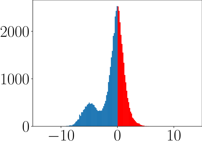
(a) Best epoch

(b) Last epoch

Figure 8: Histogram of logit margin losses of EWAT for training data on CIFAR10.

(a) AT

(b) MMA

4

(c) MART

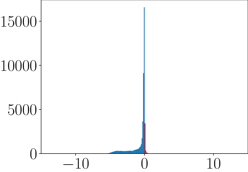
(d) GAIRAT

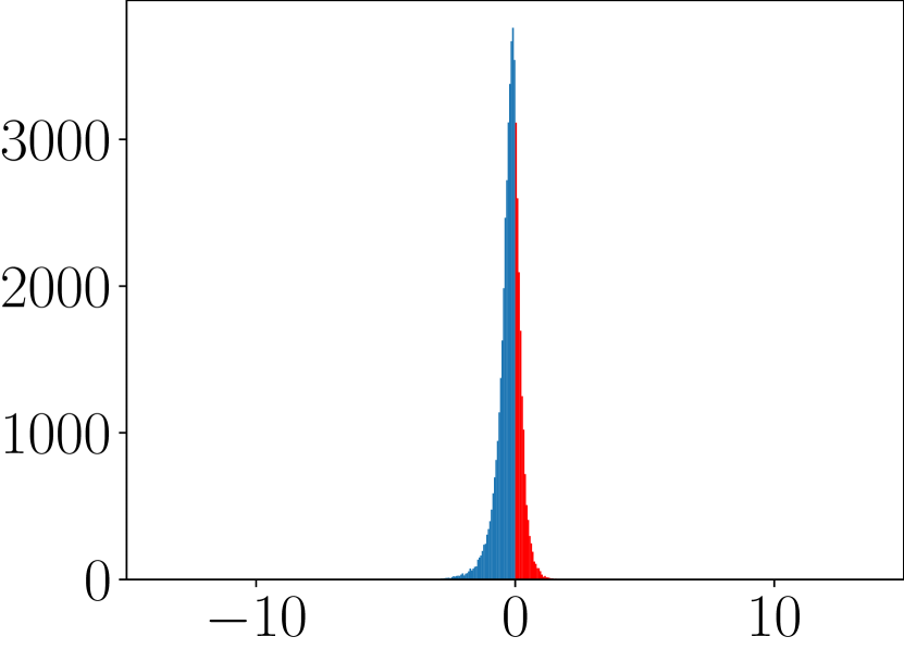
(e) MAIL

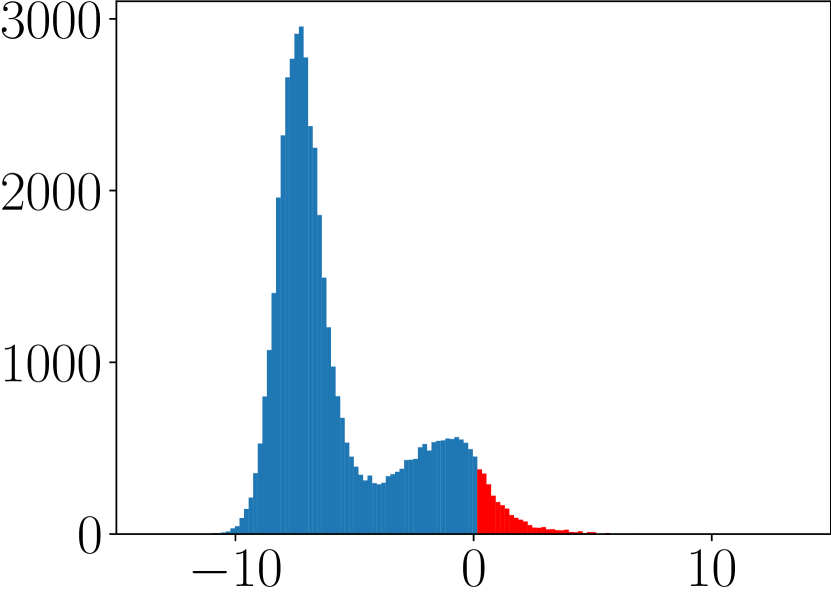
(f) EWAT

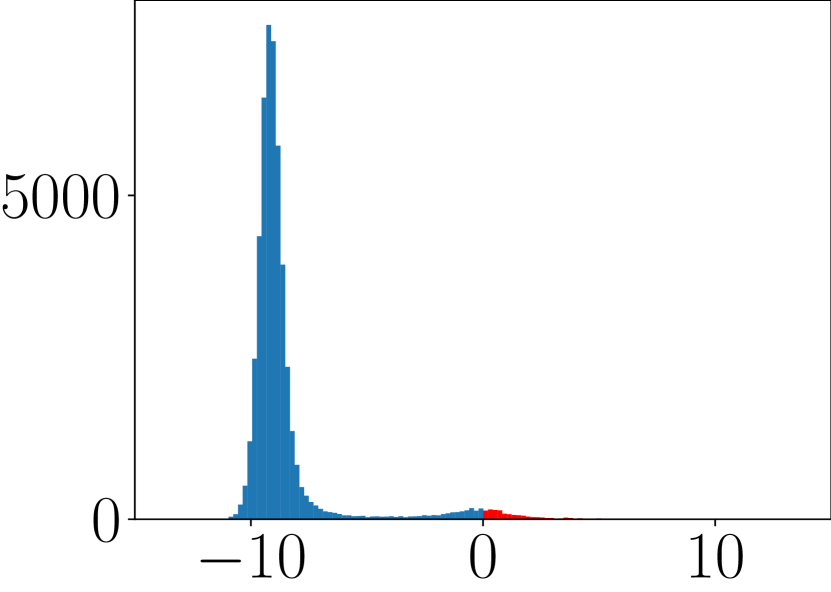
(g) SOVR

Figure 9: Histogram of logit margin losses for training samples of CIFAR10 with WideResNet34-10 at the last epoch. We plot those on adversarial data $\bm{x}^{\prime}$ for the other methods. Blue bins are the data points that models correctly classify.

(a) AT

(b) MMA

4

(c) MART

(d) GAIRAT

(e) MAIL

(f) EWAT

(g) SOVR

Figure 10: Histogram of logit margin losses for training samples of CIFAR100 at the last epoch. We plot those on adversarial data $\bm{x}^{\prime}$ for the other methods. Blue bins are the data points that models correctly classify.

(a) AT

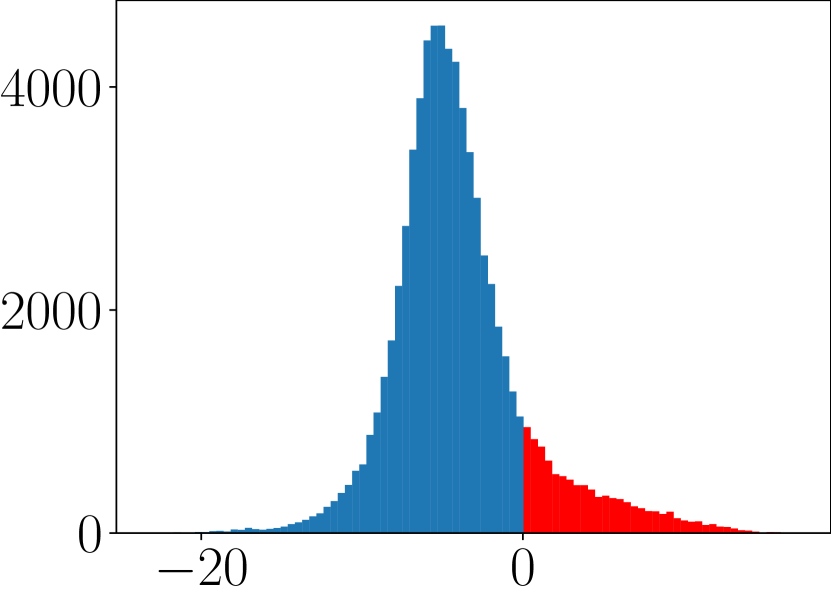
(b) MMA

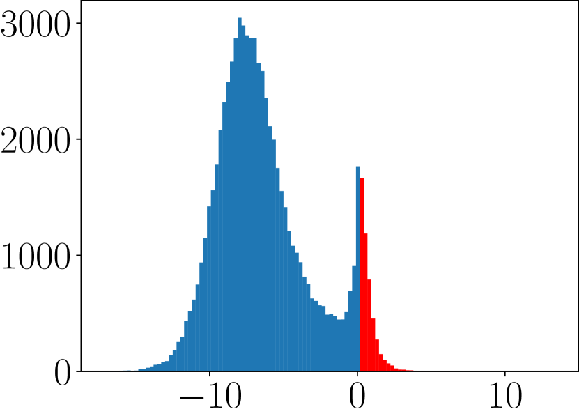
(c) MART

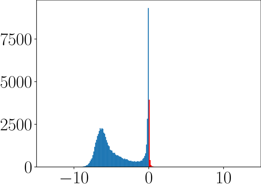
(d) GAIRAT

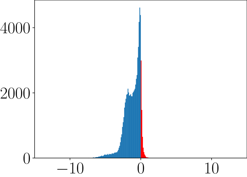
(e) MAIL

(f) EWAT

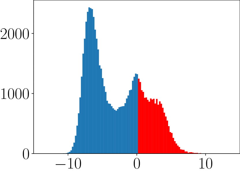
(g) SOVR

Figure 11: Histogram of logit margin losses for training samples of SVHN at the last epoch. We plot those on adversarial data $\bm{x}^{\prime}$ for the other methods. Blue bins are the data points that models correctly classify.

(a) AT

(b) MMA

(c) MART

(d) GAIRAT

(e) MAIL

(f) EWAT

(g) SOVR

Figure 12: Histogram of logit margin losses for training samples of SVHN at the 100-th epoch. We plot those on adversarial data $\bm{x}^{\prime}$ for the other methods. Blue bins are the data points that models correctly classify.

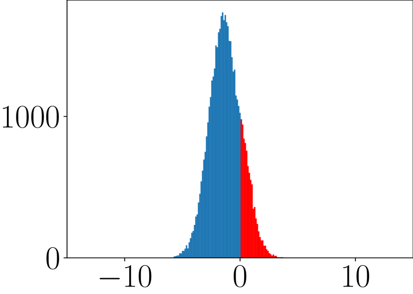
(a) Best epoch

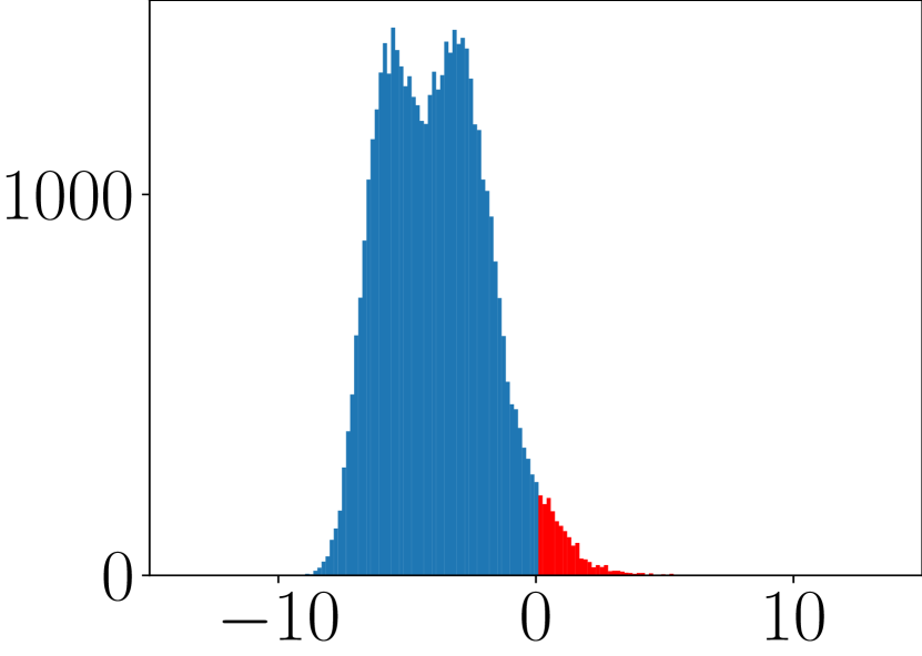
(b) Last epoch

Figure 13: Histogram of logit margin losses on CIFAR10 with WRN for TRADES.

Table 3: Average logit margin losses for training dataset $\bm{x}^{\prime}$ at the last epoch.

Dataset	AT	MART	MMA	GAIRAT	MAIL	EWAT	SOVR
CIFAR10 (RN18)	-3.66$\pm$0.02	-3.46$\pm$0.02	0.558$\pm$0.1	-0.258$\pm$ 0.02	-0.0293$\pm$ 0.02	-2.251$\pm$0.007	-4.34$\pm$ 0.02
CIFAR10 (WRN)	-6.96$\pm$0.01	-5.65$\pm$0.7	-2.73$\pm$0.6	-0.717$\pm$ 0.03	-0.203$\pm$ 0.01	-5.69$\pm$0.04	-8.56$\pm$ 0.04
CIFAR100	-2.41$\pm$0.02	-1.76$\pm$0.01	2.07$\pm$0.06	-0.68$\pm$0.02	0.684$\pm$0.1	-1.36$\pm$0.02	-2.44$\pm$0.1
SVHN	-7.55$\pm$0.01	-8.08$\pm$2	-4.31$\pm$0.04	-3.91$\pm$0.01	-1.17$\pm$0.03	-9.32$\pm$0.04	-7.59$\pm$0.1

F.2 Evaluation of Gradient Norms

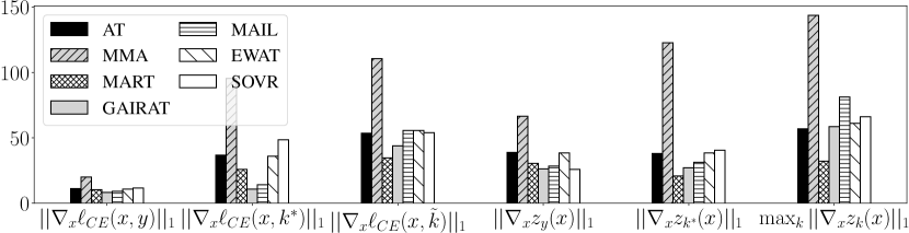
Figure 14: Average of gradient norms with respect to data points. $\tilde{k}$ is randomly selected labels, and $k^{*}\!=\!\mathrm{arg}\!\max_{k\neq y}z_{k}(\bm{x})$.

Even though logit margins of importance-aware methods are very small, they are robust against PGD and some attacks (Fig. 1). To reveal the cause of this robustness, we additionally evaluate th gradient norms for loss and logit functions (Fig. 14). In this figure, the gradient norms of cross-entropy $||\nabla_{x}\ell_{\mathrm{CE}}(\bm{x},y)||_{1}$ are relatively small values in all methods. This indicates that adversarial training essentially attempts to suppress the gradient norms for the cross-entropy. MMA has the largest gradient norms, and this is the reason MMA is not robust against Auto-Attack except for SQUARE (Fig. 1), which does not use gradient. GAIRAT and MAIL have the smallest and second smallest $||\nabla_{x}\ell_{\mathrm{CE}}(\bm{x},y)||_{1}$, and this is the reason they are robust against PGD despite the small logit margins (Fig. 2). On the other hand, $\max_{k}||\nabla_{x}z_{k}(\bm{x})||_{1}$ of importance-aware methods is larger than $||\nabla_{x}\ell_{\mathrm{CE}}(\bm{x},y)||_{1}$ of them and that of AT. As a result, they can have larger rate of potentially misclassified samples (Fig. 6). Gradient norms of cross-entropy for the label that has the largest logit except for the true label $||\nabla_{x}\ell_{\mathrm{CE}}(\bm{x},k^{*})||_{1}$ are smaller than those for the randomly selected labels. This implies $k^{*}\neq\hat{k}$, and we need to use the loss that depends on the logits for all classes rather than logit margin loss, which only cares $z_{k}^{*}$ and $z_{y}$. Gradient norms of EWAT and SOVR are not significantly different from those of AT. Thus, SOVR can reduce the rate of potentially misclassified samples by large logit margins and not large gradient norm.

F.3 Trajectories of Logit Margin Losses in Adversarial Training with OVR and Cross-entropy

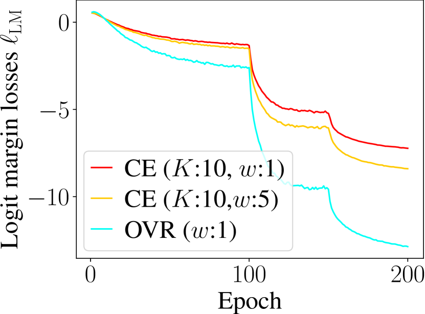
(a) CIFAR 10 (WRN)

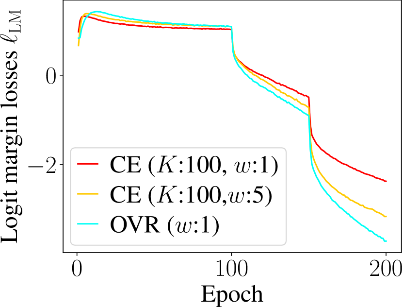
(b) CIFAR 100

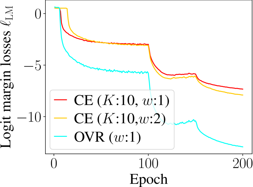
(c) SVHN

Figure 15: Trajectories of logit margin losses $\ell_{\mathrm{LM}}$ in adversarial training using cross-entropy and OVR. RN18 is used on CIFAR100 and SVHN.

In this section, we evaluate the trajectories of logit margin losses in adversarial training on real data. Experimental setup is the same with that of Section 6 except for the learning rate on CIFAR10, and thus, we minimize the OVR and cross-entropy averaged over the dataset, unlike Eq. (10). While the learning rates are set to 0.1 for cross-entropy and 0.05 for SOVR in Section 6 on CIFAR10, learning rate is set to 0.05 on CIFAR10 for both cross-entropy and OVR to fairly compare their logit margin losses in this experiment. Since we could not obtain results on SVHN with the weight of $w\!=\!5$ due to unstability, we used $w\!=\!2$ on SVHN. Fig. 15 plots the logit margin losses averaged over the dataset against epochs in adversarial training with OVR and cross-entropy on CIFAR10, CIFAR100, and SVHN. In Fig. 15, OVR decreases the logit margin losses more than cross-entropy on all dataset. We also evaluate $\ell_{\mathrm{LM}}(\bm{z}^{OVR})/\ell_{\mathrm{LM}}(\bm{z}^{CE})$ at the last epoch, which is expected to be about two from Theorem 4.5. Table 4 list $\ell_{\mathrm{LM}}(\bm{z}^{OVR})/\ell_{\mathrm{LM}}(\bm{z}^{CE})$ at the last epoch, and it is about two, and thus, logit margin losses in adversarial training follow Theorem 4.5 well even though we assume a simple problem that only considers one data point and assumes that logits are directly moved by the gradient for Theorem 4.5. Since the number of classes $K$ of CIFAR100 is 100 and larger than other datasets, the logit margins of cross-entropy is larger than OVR at the beginning of training. This result corresponds to the case of CE ($K=100$) in Fig. 3(a), and this phenomenon is also able to be explained by the simple problem Eq. (10). To the best of our knowledge, this is the first study that explicitly reveals the logit margin of minimization of cross-entropy depends on the number of classes. Though the logit margin loss of OVR in Theorem 4.5 does not depend on $K$, the logit margins of OVR on CIFAR100 is smaller than those on CIFAR10 and SVHN. This is because CIFAR100 is a more difficult dataset than CIFAR10 and SVHN: robust accuracies of CIFAR100 is about 25 % whereas those of CIFAR10 and SVHN are about 50 % in Tab. 1.

CIFAR10 (RN18)	CIFAR10 (WRN)	CIFAR100	SVHN
1.87	1.78	1.56	1.76

Table 4: $\ell_{\mathrm{LM}}(\bm{z}^{OVR})/\ell_{\mathrm{LM}}(\bm{z}^{CE})$ with $w=1.0$ at the last epoch

F.4 Effects of Hyperparameters $\lambda$

SOVR has hyperparameters ($M$, $\lambda$). In this section, we evaluate the effects of $\lambda$. Figure 16 plots $\ell_{LM}$ on CIFAR10 with RN18, generalization gap, and robust accuracy against Auto-Attack. We set $M$ to 40. Note that $\lambda=0$ corresponds to that models are trained on only a set of $\mathbb{S}$, i.e., AT only using the 60 percent of the data points in minibatch when $M=40$. First, $\ell_{LM}(\bm{x}^{\prime})$ is monotonically decreasing due to increases in $\lambda$ (Fig. 16(a)). However, robust accuracies against Auto-Attack are not monotonically increasing against $\lambda$ (Fig. 16(c)). This is because generalization gap increases (Fig. 16(b)). Thus, too high weights on important samples causes overfitting. SOVR is always superior or comparable to AT in terms of robustness against Auto-Attack under all tested values of ($0<M\leq 100$, $0<\lambda\leq 1$).

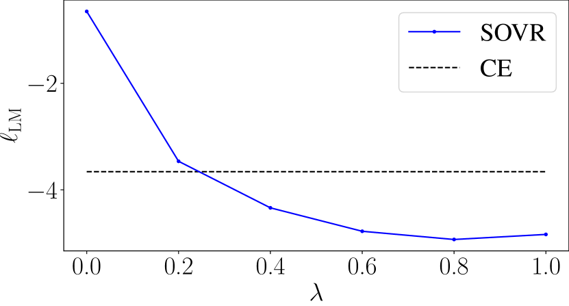
(a) $\ell_{\mathrm{LM}}(\bm{x}^{\prime})$ Vs $\lambda$

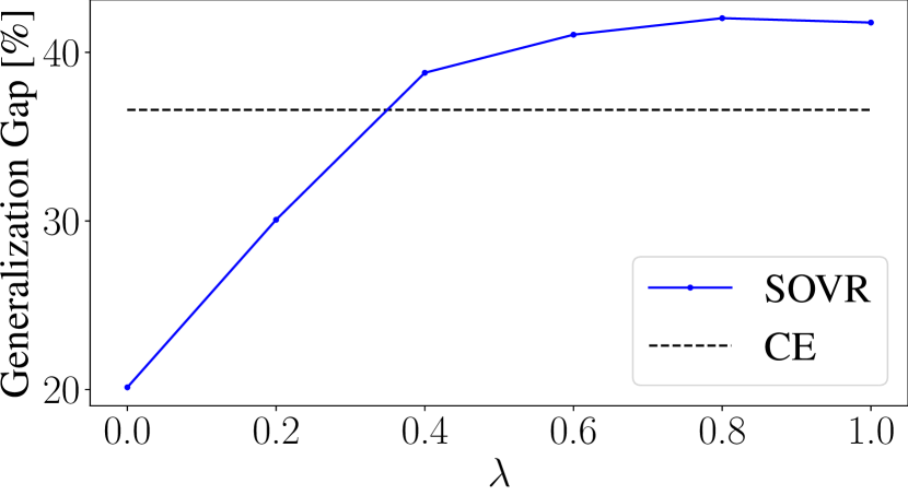
(b) Generalization Gap Vs $\lambda$

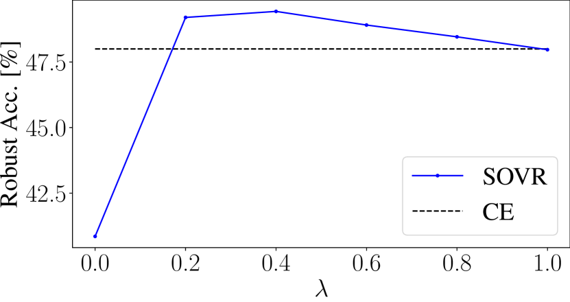
(c) Robust Acc. Vs $\lambda$

Figure 16: The effect of rate of applying OVR $\lambda$. $M$ is set to 40. Generalization gap is a gap between training robust accuracy and test robust accuracy against PGD ($\mathcal{K}$=20) at the last epoch. Robust Acc. is robust accuracy against Auto-Attack. Dashed gray line corresponds to the results of AT using cross-entropy loss.

F.5 Individually Test of Auto-Attack

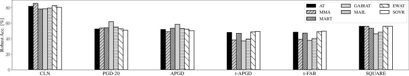
Figure 17: The robustness against PGD-20 and Auto-Attack on the test set of CIFAR10. We decompose the robust accuracy for Auto-Attack into robust accuracy in each phase.

For importance-aware methods, we evaluate the robust accuracies against all components of Auto-Attack in Section 2.3. In this section, we additionally evaluate EWAT by individually using Auto-Attack and discuss the results of SOVR. Figure 17 plots the results, and SOVR is the most robust against t-APG and t-FABand. In addition, it is more robust against SQUARE than AT and EWAT. Although the robust accuracy of SOVR against PGD-20 is lower than those of AT and EWAT, SOVR outperforms other methods in terms of the robustness against the worst-case attacks, which is the goal of this study.

F.6 Evaluation Using Various Attacks

We list robust accuracies against various attacks; FGSM (Goodfellow et al., 2014), 100-step PGD (Madry et al., 2018), 100-step PGD with CW loss (Madry et al., 2018; Carlini & Wagner, 2017), SPSA (Uesato et al., 2018) in Tab. F.6. Hyperparameters of SPSA are as follows: the number of steps is set to 100, the perturbation size is set to 0.001, learning rate is set to 0.01, and the number of samples for each gradient estimation is set to 256. In this table, we repeat the clean accuracies and robust accuracies against Auto-Attack from the table in the main paper. In addition, we list the worst robust accuracies, which are the least robust accuracy among attacks in the table for each method. In this table, importance-aware methods tend to fail to improve the robustness against SPSA. Since SPSA does not directly use gradients, this result indicates that importance-aware methods improve the robustness by obfuscating gradients (Athalye et al., 2018). Against some attacks, MMA achieves the highest robust accuracy on several datasets. However, our goal is improving the true robustness, i.e., robust accuracies against the worst-case attacks in $\bm{\delta}\in\{||\bm{\delta}||_{\infty}\leq 8/255\}$. MMA does not improve the robustness against the worst-case attacks (the columns of Worst). We can see that Auto-Attack always achieves the least robust accuracies, and SOVR improves them: Robust accuracies against Auto-Attack of SOVR are 5.9-12.2 percent points greater than those of MMA.

Table 5: Robust Accuracy against various attacks ($L_{\infty}$, $\varepsilon=8/255$). CLN denotes accuracy on clean data, and AA denotes Auto-Attack. Worst represents the least robust accuracy among attacks in the table for each method.

	Method	CLN	FGSM	PGD	CW	SPSA	AA	Worst
	AT	81.6$\pm$0.5	57.6$\pm$0.1	52.5$\pm$0.4	50.0$\pm$0.4	56.8$\pm$0.2	48.0$\pm$0.2	48.0$\pm$0.2
	MART	78.3$\pm$1	58.0$\pm$0.3	54.0$\pm$0.1	48.7$\pm$0.2	54.2$\pm$0.1	46.9$\pm$0.3	46.9$\pm$0.3
	MMA	$\bm{85.5\pm 0.7}$	$\bm{65.5\pm 2}$	51.6$\pm$0.2	51.0$\pm$0.6	56.3$\pm$1	37.2$\pm$0.9	37.2$\pm$0.9
C10	GAIRAT	78.7$\pm$0.7	63.1$\pm$0.7	$\bm{62.0\pm 0.4}$	40.01$\pm$1	47.4$\pm$1	37.7$\pm$1	37.7$\pm$1
(RN18)	MAIL	79.5$\pm$0.4	57.8$\pm$0.1	54.97$\pm$0.08	42.1$\pm$0.2	49.1$\pm$0.4	39.6$\pm$0.4	39.6$\pm$0.4
	EWAT	82.8$\pm$0.4	57.7$\pm$0.4	52.3$\pm$0.4	50.4$\pm$0.7	56.8$\pm$0.2	48.2$\pm$0.7	48.2$\pm$0.7
	SOVR	81.9$\pm$0.2	57.0$\pm$0.2	50.9$\pm$0.5	$\bm{51.5\pm 0.2}$	$\bm{57.7\pm 0.2}$	$\bm{49.4\pm 0.3}$	$\bm{49.4\pm 0.3}$
	AT	85.6$\pm$0.5	60.9$\pm$0.4	55.1$\pm$0.4	54.0$\pm$0.6	60.8$\pm$0.5	51.9$\pm$0.5	51.9$\pm$0.5
	MART	81.5$\pm$1	61.3$\pm$0.6	57.2$\pm$0.2	52.1$\pm$0.3	57.8$\pm$0.6	50.44$\pm$0.09	50.44$\pm$0.09
	MMA	$\bm{87.8\pm 1}$	$\bm{68.6\pm 1}$	55.7$\pm$1	$\bm{55.4\pm 0.7}$	59.6$\pm$2	43.1$\pm$0.6	43.1$\pm$0.6
C10	GAIRAT	83.0$\pm$0.7	64.1$\pm$0.5	$\bm{62.9\pm 0.4}$	44.4$\pm$0.7	52.1$\pm$0.5	41.8$\pm$0.6	41.8$\pm$0.6
(WRN)	MAIL	82.2$\pm$0.4	59.3$\pm$0.5	56.0$\pm$0.5	45.7$\pm$0.2	53.0$\pm$0.2	43.3$\pm$0.1	43.3$\pm$0.1
	EWAT	86.0$\pm$0.5	60.6$\pm$0.4	54.5$\pm$0.1	53.8$\pm$0.3	60.7$\pm$0.4	51.6$\pm$0.3	51.6$\pm$0.3
	SOVR	85.0$\pm$1	60.8$\pm$0.1	54.5$\pm$0.2	55.2$\pm$0.2	$\bm{61.6\pm 0.1}$	$\bm{53.1\pm 0.2}$	$\bm{53.1\pm 0.2}$
	AT	89.8$\pm$0.6	30.1$\pm$0.4	27.7$\pm$0.2	25.6$\pm$0.3	29.3$\pm$0.3	23.7$\pm$0.3	23.7$\pm$0.3
	MART	86.9$\pm$0.6	$\bm{31.0\pm 0.2}$		25.4$\pm$0.3	28.5$\pm$0.1	23.9$\pm$0.3	23.9$\pm$0.3
	MMA	$\bm{93.9\pm 0.4}$	25.7$\pm$0.3	19.4$\pm$0.2	20.5$\pm$0.1	24.3$\pm$0.3	18.4$\pm$0.2	18.4$\pm$0.2
C100	GAIRAT	89.9$\pm$0.4	27.9$\pm$0.3	26.0$\pm$0.2	21.9$\pm$0.4	25.9$\pm$0.1	19.8$\pm$0.5	19.8$\pm$0.5
	MAIL	89.4$\pm$0.4	24.81$\pm$0.08	23.29$\pm$0.06	18.3$\pm$0.5	21.9$\pm$0.5	16.7$\pm$0.3	16.7$\pm$0.3
	EWAT	90.2$\pm$0.6	30.07$\pm$0.08	27.4$\pm$0.3	25.3$\pm$0.2	29.3$\pm$0.1	23.52$\pm$0.06	23.52$\pm$0.06
	SOVR	90.0$\pm$1	30.2$\pm$0.2	27.4$\pm$0.2	$\bm{26.1\pm 0.1}$	$\bm{29.9\pm 0.1}$	$\bm{24.3\pm 0.2}$	$\bm{24.3\pm 0.2}$
	AT	53.0$\pm$0.7	61.1$\pm$0.5	50.6$\pm$0.4	47.7$\pm$0.8	55.7$\pm$0.9	45.6$\pm$0.4	45.6$\pm$0.4
	MART	49.2$\pm$0.1	64.4$\pm$0.5	56.5$\pm$0.2	49.0$\pm$0.4	56.69$\pm$0.08	46.9$\pm$0.3	46.9$\pm$0.3
	MMA	$\bm{60.6\pm 0.6}$		$\bm{65.0\pm 1}$	$\bm{59.1\pm 2}$	$\bm{63.2\pm 2}$	41.0$\pm$0.3	41.0$\pm$0.3
SVHN	GAIRAT	52.0$\pm$0.5	65.8$\pm$0.4	60.4$\pm$0.6	40.6$\pm$0.7	48.8$\pm$0.6	37.6$\pm$0.6	37.6$\pm$0.6
	MAIL	46.5$\pm$0.5	64.6$\pm$0.4	58.2$\pm$0.3	44.1$\pm$0.7	52.3$\pm$0.5	41.2$\pm$0.3	41.2$\pm$0.3
	EWAT	54.2$\pm$1	61.8$\pm$0.5	51.7$\pm$0.2	50.2$\pm$0.4	57.4$\pm$0.4	47.6$\pm$0.4	47.6$\pm$0.4
	SOVR	52.1$\pm$0.8	65.3$\pm$2	50.7$\pm$0.2	52.5$\pm$0.2	60.7$\pm$0.4	$\bm{48.5\pm 0.4}$	$\bm{48.5\pm 0.4}$

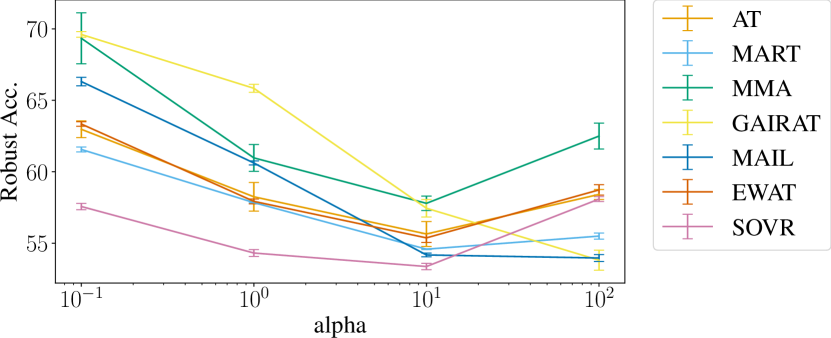
(a) CIFAR10 (RN18)

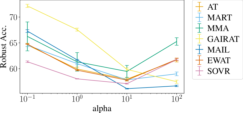
(b) CIFAR10 (WRN)

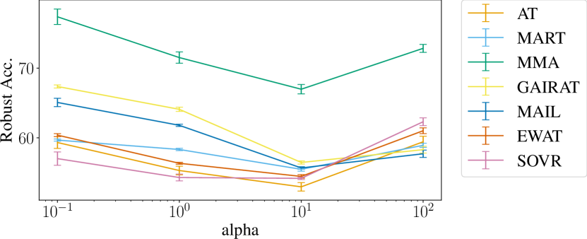
(c) SVHN

(d) CIFAR100

Figure 18: Robust Accuracy against logit scaling attack.

F.7 Evaluation using Logit Scaling Attack

In this section, we evaluate the robustness against the logit scaling attack (Hitaj et al., 2021). Hitaj et al. (2021) reveals that GAIRAT tends to be vulnerable to logit scaling attacks. The logit scaling attack multiplies logits by $\alpha$ before applying softmax when generating PGD attacks. We set $\alpha=[0.1,1.0,10,100]$. Fig. 18 plots robust accuracy against $\alpha$. This figure shows that the robust accuracies of GAIRAT and MAIL tend to decrease when increasing $\alpha$. Though the robust accuracy of SOVR is the lowest on CIFAR 10 (RN18), it is higher than the robust accuracy against Auto-Attack. Thus, the logit scaling attack is not the worst-case attack. Since the robust accuracy of SOVR does not necessarily decrease when increasing $\alpha$, the results seem to be caused by high robustness against PGD (Tab. F.6) of other methods rather than vulnerability to logit scaling of SOVR. Previous methods tend to be designed to increase the robustness against PGD since Auto-Attack is a relatively recent attack. On the other hand, SOVR is designed to increase the robustness against the worst-case attack, which is Auto-Attack for now.

F.8 Evaluation using Auto-Attack with larger magnitudes

In this section, we evaluate the robustness against Auto-Attack with $\varepsilon=12/255$ and $16/255$. These magnitudes are larger than the magnitude used in adversarial training, and thus, this experiment evaluates the existence of overfitting to the magnitude used in training. Tab. 6 lists robust accuracies against Auto-Attack with $\varepsilon=12/255$ and $16/255$. This table shows that SOVR outperforms AT, and TSOVR achieves the largest robust accuracies. Thus, our methods do not overfit to the magnitude of attacks used in training. Interestingly, this table also shows that MART outperforms AT while the robust accuracies against $\varepsilon\!=\!8/255$ of MART are not always larger than those of AT (Tab. 1). MART might have better generalization performance for the magnitudes of attacks.

Table 6: Robust accuracy against Auto-Attack using $\varepsilon=12/255$ and $16/255$.

Robust Accuracy against Auto-Attack ($L_{\infty}$, adversarialy trained by using PGD with $\varepsilon\!=\!8/255$)
	AT	MART	MMA	GAIRAT	MAIL	EWAT	SOVR	TRADES	TSOVR
CIFAR10 (RN18, $\varepsilon\!=\!12/255$)	28.6$\pm$0.6	29.6$\pm$0.8	19.7$\pm$0.9	19$\pm$1	20.2$\pm$0.5	28.4$\pm$0.8	30.3$\pm$0.3	30.6$\pm$0.5	$\bm{31.9\pm 0.4}$
CIFAR10 (RN18, $\varepsilon\!=\!16/255$)	13.6$\pm$0.6	15$\pm$1	8.8$\pm$0.5	7.8$\pm$0.5	7.9$\pm$0.5	13.2$\pm$0.2	14.3$\pm$0.1	16.0$\pm$0.8	$\bm{17.0\pm 0.5}$
CIFAR10 (WRN, $\varepsilon\!=\!12/255$)	31.2$\pm$0.2	32$\pm$1	25$\pm$1	22$\pm$1	23.0$\pm$0.2	31.1$\pm$0.3	32.7$\pm$0.3	34.8$\pm$0.2	$\bm{35.5\pm 0.3}$
CIFAR10 (WRN, $\varepsilon\!=\!16/255$)	15.3$\pm$0.3	17$\pm$1	13$\pm$1	9.1$\pm$0.7	9.43$\pm$0.4	14.8$\pm$0.1	16.1$\pm$0.4	19.6$\pm$0.1	$\bm{20.4\pm 0.6}$
SVHN (RN18, $\varepsilon\!=\!12/255$)	23.0$\pm$0.5	24$\pm$1	23$\pm$1	18.2$\pm$0.7	19$\pm$1	25.9$\pm$0.7	25$\pm$1	29.0$\pm$0.6	$\bm{29.4\pm 0.5}$
SVHN (RN18, $\varepsilon\!=\!16/255$)	10.6$\pm$0.5	11.4$\pm$0.7	14$\pm$1	7.9$\pm$0.3	8.1$\pm$0.2	12.0$\pm$0.4	10.5$\pm$0.6	15.2$\pm$0.7	$\bm{15.4\pm 0.7}$
CIFAR100 (RN18, $\varepsilon\!=\!12/255$)	13.8$\pm$0.1	15.2$\pm$0.3	10.0$\pm$0.3	10.45$\pm$0.5	8.5$\pm$0.4	13.4$\pm$0.1	14.5$\pm$0.3	13.9$\pm$0.3	$\bm{16.0\pm 0.2}$
CIFAR100 (RN18, $\varepsilon\!=\!16/255$)	7.53$\pm$0.03	9.4$\pm$0.1	5.9$\pm$0.3	5.1$\pm$0.4	4.1$\pm$0.4	7.1$\pm$0.1	8.1$\pm$0.1	8.2$\pm$0.1	$\bm{10.0\pm 0.1}$

F.9 Dependence of the Number of Classes

Figure 6 shows that the rate of AT gets close to SOVR on CIFAR100. This is because the number of classes of CIFAR100 ($K=100$) is ten times larger than other datasets ($K=10$), and logit margins of cross-entropy depend on the number of classes $K$ (Eq. (17)). Thus, this result is a piece of evidence that Theorem 4.5 explains the difference of logit margins between OVR and cross-entropy. In certain finite time step $t$ (not the limit), Eqs. (16) and (17) show that the difference between OVR and cross-entropy depends on the number of classes $K$. Even so, Fig. 15(b) shows that the increase rate of logit margins of OVR is larger than that of cross-entropy against epochs. To achieve better performance, we can tune the hyper-parameter $\lambda$, which corresponds to $w_{1}$ in Eq. (16) of Theorem 4.5. When using $\lambda$= 0.6, SOVR achieves better robustness than $\lambda=0.5$ on CIFAR100 (Tab. 7). Cross-entropy also has the weight $w_{2}$ in Eq. (17), and it is automatically tuned in GAIRAT, MAIL, and EWAT. However, this tuning does not achieve comparable performance to SOVR.

Table 7: Robust accuracy against Auto-Attack on CIFAR100 tuning $\lambda$.

Robust Accuracy against Auto-Attack ($L_{\infty}$, $\varepsilon\!=\!8/255$)
	AT	SOVR ($\lambda$=0.5)	SOVR ($\lambda$=0.6)
CIFAR100 (RN18)	23.7$\pm$0.3	24.3$\pm$0.2	$\bm{24.6\pm 0.1}$
Clean Accuracy
CIFAR100 (RN18)	$\bm{53.0\pm 0.7}$	52.1$\pm$0.8	51.9 $\pm$ 0.6

F.10 Histogram of Probabilistic Margin Losses

While our study focuses on the logit margin loss, MAIL (Liu et al., 2021) uses the probabilistic margin,

$$\textstyle PM_{n} \textstyle=f_{y_{n}}(\bm{x}_{n}^{\prime},\bm{\theta})-\max_{k\neq{y_{n}}}f_{k}(\bm{x}_{n}^{\prime},\bm{\theta}),$$ (89)

to evaluate the difficulty of data point. In the same way as Fig. 2, Fig. 19 plots the histograms of probabilistic margins on CIFAR10 with PreActResNet18. Since softmax output is bounded in $[0,1]$, $PM$ is bounded in [-1,1]. As a result, most correctly classified data points concentrate near -1. In addition, softmax uses exponential functions, distributions of $PM$ are similar to the exponential distributions. Due to these effects, histograms of $PM$ make it more difficult to discover the fact that there are two types of data points (easy samples and difficult samples). Since softmax preserves the order of logit, and a classifier infers the label by using the largest logit, the analysis by using $PM$ can under-estimate the distribution of difficult samples. Thus, logit margin losses are more suitable to empirically analyze trained models. Since softmax preserves the order of logit, the probabilistic margin can be used to determine $\mathbb{L}$ and $\mathbb{S}$ in SOVR.

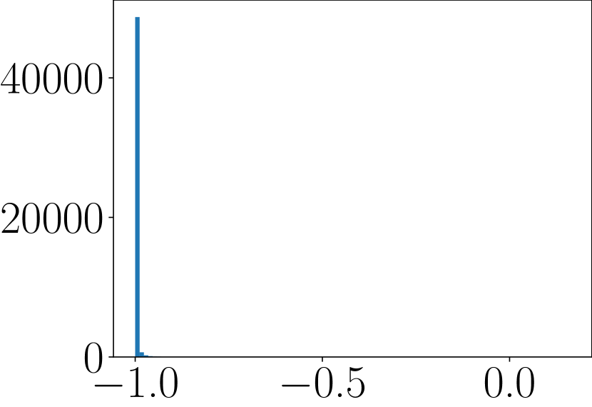
(a) ST

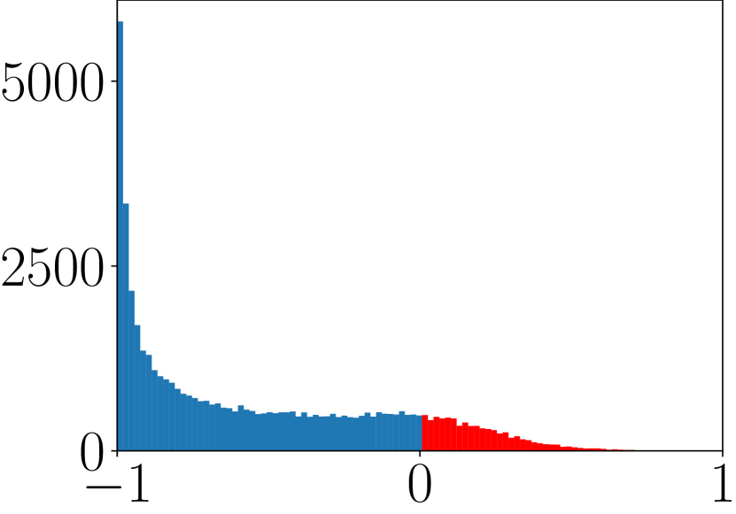
(b) AT

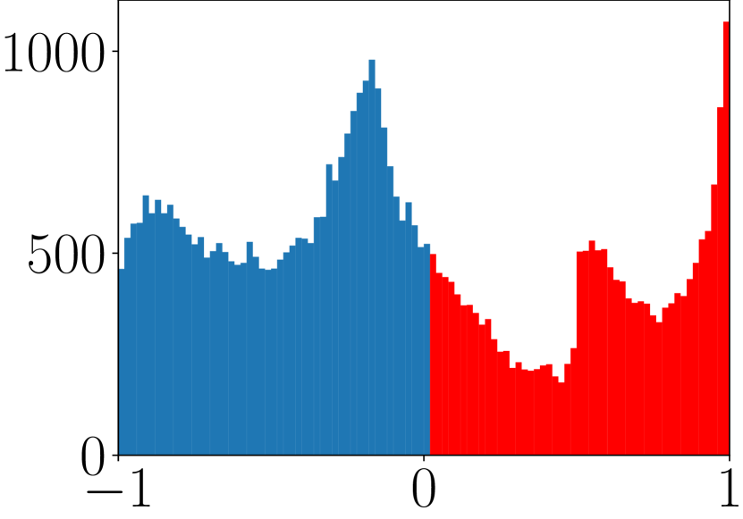
(c) MMA

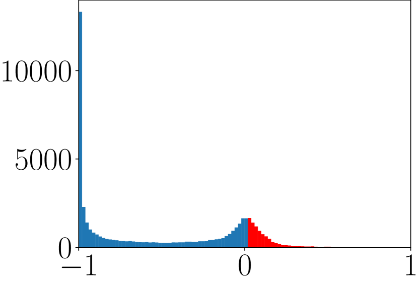
(d) MART

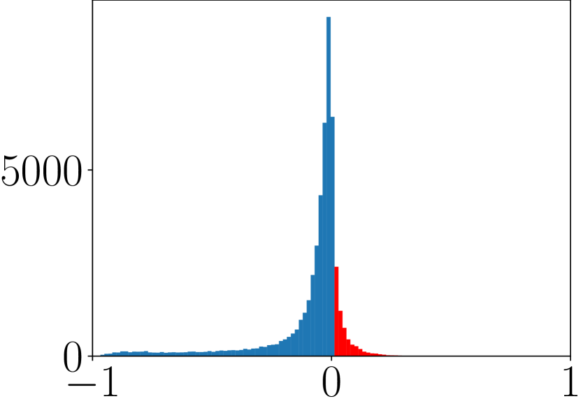
(e) GAIRAT

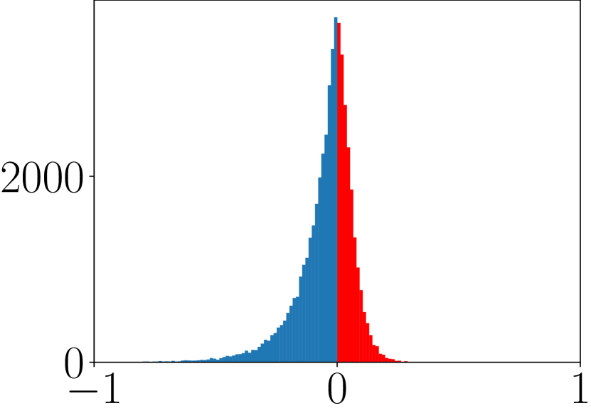
(f) MAIL

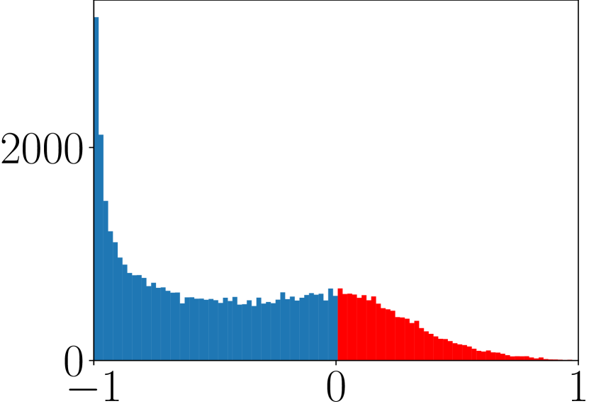
(g) EWAT

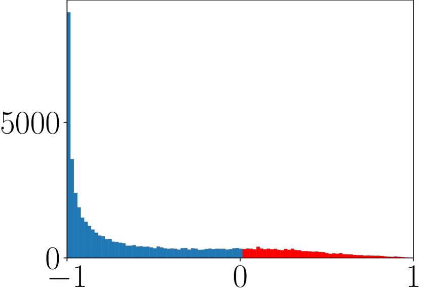
(h) SOVR

Figure 19: Histogram of probabilistic margin losses for training data of CIFAR10 with PreActResNet18 at the last epoch. ST denotes standard training, i.e., training on clean data. For standard training, we use $PM$ on clean data $\bm{x}$, while we plot that on adversarial examples $\bm{x}^{\prime}$ for the other methods. Blue bins correspond to the correctly classified data points, and red bins are misclassified samples.

References

- Athalye et al. (2018) Athalye, A., Carlini, N., and Wagner, D. Obfuscated gradients give a false sense of security: Circumventing defenses to adversarial examples. In Proc. ICML, pp. 274–283, 2018.
- Bartlett et al. (2003) Bartlett, P. L., Jordan, M. I., and McAuliffe, J. D. Convexity, classification, and risk bounds. 2003.
- Carlini & Wagner (2017) Carlini, N. and Wagner, D. Towards evaluating the robustness of neural networks. In 2017 IEEE Symposium on Security and Privacy (SP), pp. 39–57. IEEE, 2017.
- Carmon et al. (2019) Carmon, Y., Raghunathan, A., Schmidt, L., Duchi, J. C., and Liang, P. S. Unlabeled data improves adversarial robustness. In Proc. NeurIPS, pp. 11190–11201, 2019.
- Cisse et al. (2017) Cisse, M., Bojanowski, P., Grave, E., Dauphin, Y., and Usunier, N. Parseval networks: Improving robustness to adversarial examples. In Proc. ICML, pp. 854–863, 2017.
- Cohen et al. (2019) Cohen, J., Rosenfeld, E., and Kolter, Z. Certified adversarial robustness via randomized smoothing. In Proc. ICML, pp. 1310–1320, 2019.
- Corless et al. (1996) Corless, R. M., Gonnet, G. H., Hare, D. E., Jeffrey, D. J., and Knuth, D. E. On the lambertw function. Advances in Computational mathematics, 5(1):329–359, 1996.
- Croce & Hein (2020) Croce, F. and Hein, M. Reliable evaluation of adversarial robustness with an ensemble of diverse parameter-free attacks. In Proc. ICML, 2020.
- Ding et al. (2020) Ding, G. W., Sharma, Y., Lui, K. Y. C., and Huang, R. Mma training: Direct input space margin maximization through adversarial training. In Proc. ICLR, 2020.
- Dong et al. (2022) Dong, Y., Xu, K., Yang, X., Pang, T., Deng, Z., Su, H., and Zhu, J. Exploring memorization in adversarial training. In Proc. ICLR, 2022.
- Elkabetz & Cohen (2021) Elkabetz, O. and Cohen, N. Continuous vs. discrete optimization of deep neural networks. Proc. NeurIPS, 34:4947–4960, 2021.
- Goodfellow et al. (2014) Goodfellow, I., Shlens, J., and Szegedy, C. Explaining and harnessing adversarial examples. arXiv preprint arXiv:1412.6572, 2014.
- Gowal et al. (2021) Gowal, S., Rebuffi, S.-A., Wiles, O., Stimberg, F., Calian, D. A., and Mann, T. Improving robustness using generated data. arXiv preprint arXiv:2110.09468, 2021. URL https://arxiv.org/pdf/2110.09468.
- He et al. (2016) He, K., Zhang, X., Ren, S., and Sun, J. Deep residual learning for image recognition. In Proc. CVPR, pp. 770–778, 2016.
- Hitaj et al. (2021) Hitaj, D., Pagnotta, G., Masi, I., and Mancini, L. V. Evaluating the robustness of geometry-aware instance-reweighted adversarial training. arXiv preprint arXiv:2103.01914, 2021.
- Hoorfar & Hassani (2007) Hoorfar, A. and Hassani, M. Approximation of the lambert w function and hyperpower function. Research report collection, 10(2), 2007.
- Jordan & Dimakis (2020) Jordan, M. and Dimakis, A. G. Exactly computing the local lipschitz constant of relu networks. Proc. NeurIPS, 33:7344–7353, 2020.
- Kim et al. (2021) Kim, M., Tack, J., Shin, J., and Hwang, S. J. Entropy weighted adversarial training. In ICML 2021 Workshop on Adversarial Machine Learning, 2021.
- Krizhevsky & Hinton (2009) Krizhevsky, A. and Hinton, G. Learning multiple layers of features from tiny images. Technical report, 2009.
- Kunin et al. (2021) Kunin, D., Sagastuy-Brena, J., Ganguli, S., Yamins, D. L., and Tanaka, H. Neural mechanics: Symmetry and broken conservation laws in deep learning dynamics. In Proc. ICLR, 2021.
- Kurakin et al. (2016) Kurakin, A., Goodfellow, I., and Bengio, S. Adversarial machine learning at scale. arXiv preprint arXiv:1611.01236, 2016.
- Lin (2002) Lin, Y. Support vector machines and the bayes rule in classification. Data Mining and Knowledge Discovery, 6(3):259–275, 2002.
- Liu et al. (2021) Liu, F., Han, B., Liu, T., Gong, C., Niu, G., Zhou, M., Sugiyama, M., et al. Probabilistic margins for instance reweighting in adversarial training. Proc. NeurIPS, 34, 2021.
- Madry et al. (2018) Madry, A., Makelov, A., Schmidt, L., Tsipras, D., and Vladu, A. Towards deep learning models resistant to adversarial attacks. In Proc. ICLR, 2018.
- Netzer et al. (2011) Netzer, Y., Wang, T., Coates, A., Bissacco, A., Wu, B., and Ng, A. Y. Reading digits in natural images with unsupervised feature learning. In NIPS Workshop on Deep Learning and Unsupervised Feature Learning, 2011.
- Padhy et al. (2020) Padhy, S., Nado, Z., Ren, J., Liu, J., Snoek, J., and Lakshminarayanan, B. Revisiting one-vs-all classifiers for predictive uncertainty and out-of-distribution detection in neural networks. In ICML Workshop on Uncertainty and Robustness in Deep Learning, 2020.
- Rade (2021) Rade, R. PyTorch implementation of uncovering the limits of adversarial training against norm-bounded adversarial examples, 2021. URL https://github.com/imrahulr/adversarial_robustness_pytorch.
- Rebuffi et al. (2021) Rebuffi, S.-A., Gowal, S., Calian, D. A., Stimberg, F., Wiles, O., and Mann, T. Fixing data augmentation to improve adversarial robustness. arXiv preprint arXiv:2103.01946, 2021. URL https://arxiv.org/pdf/2103.01946.
- Saito & Saenko (2021) Saito, K. and Saenko, K. Ovanet: One-vs-all network for universal domain adaptation. In Proceedings of the IEEE/CVF International Conference on Computer Vision, pp. 9000–9009, 2021.
- Sanyal et al. (2021) Sanyal, A., Dokania, P. K., Kanade, V., and Torr, P. How benign is benign overfitting? In Proc. ICLR, 2021.
- Schmidt et al. (2018) Schmidt, L., Santurkar, S., Tsipras, D., Talwar, K., and Madry, A. Adversarially robust generalization requires more data. Proc. NeurIPS, 31, 2018.
- Szegedy et al. (2013) Szegedy, C., Zaremba, W., Sutskever, I., Bruna, J., Erhan, D., Goodfellow, I., and Fergus, R. Intriguing properties of neural networks. arXiv preprint arXiv:1312.6199, 2013.
- Tsuzuku et al. (2018) Tsuzuku, Y., Sato, I., and Sugiyama, M. Lipschitz-margin training: Scalable certification of perturbation invariance for deep neural networks. In Proc. NeurIPS, pp. 6542–6551, 2018.
- Uesato et al. (2018) Uesato, J., O’Donoghue, B., Kohli, P., and van den Oord, A. Adversarial risk and the dangers of evaluating against weak attacks. In Proc. ICML, volume 80, pp. 5025–5034. PMLR, 2018.
- Wang & Wang (2022) Wang, H. and Wang, Y. Self-ensemble adversarial training for improved robustness. In Proc. ICLR, 2022.
- Wang et al. (2020a) Wang, Y., Zou, D., Yi, J., Bailey, J., Ma, X., and Gu, Q. Improving adversarial robustness requires revisiting misclassified examples. In Proc. ICLR, 2020a.
- Wang et al. (2020b) Wang, Y., Zou, D., Yi, J., Bailey, J., Ma, X., and Gu, Q. Improving adversarial robustness requires revisiting misclassified examples. In Proc. ICLR, 2020b.
- Wu et al. (2020) Wu, D., tao Xia, S., and Wang, Y. Adversarial weight perturbation helps robust generalization. In Proc. NeurIPS, 2020. URL https://github.com/csdongxian/AWP.
- Zagoruyko & Komodakis (2016) Zagoruyko, S. and Komodakis, N. Wide residual networks. arXiv preprint arXiv:1605.07146, 2016.
- Zhang et al. (2021a) Zhang, B., Cai, T., Lu, Z., He, D., and Wang, L. Towards certifying l-infinity robustness using neural networks with l-inf-dist neurons. In Proc. ICML, volume 139, pp. 12368–12379, 2021a.
- Zhang et al. (2019) Zhang, H., Yu, Y., Jiao, J., Xing, E., Ghaoui, L. E., and Jordan, M. Theoretically principled trade-off between robustness and accuracy. In Proc. ICML, volume 97, pp. 7472–7482. PMLR, 2019.
- Zhang et al. (2020) Zhang, J., Xu, X., Han, B., Niu, G., Cui, L., Sugiyama, M., and Kankanhalli, M. Attacks which do not kill training make adversarial learning stronger. 119:11278–11287, 2020.
- Zhang et al. (2021b) Zhang, J., Zhu, J., Niu, G., Han, B., Sugiyama, M., and Kankanhalli, M. Geometry-aware instance-reweighted adversarial training. In Proc. ICLR, 2021b.
- Zhang (2004) Zhang, T. Statistical analysis of some multi-category large margin classification methods. Journal of Machine Learning Research, 5(Oct):1225–1251, 2004.