Triaxiality explored by an odd quasi-particle

Abstract

The triaxiality of odd-mass nuclei is investigated by coupling a quasiparticle to an even-even core through the core-quasiparticle coupling model. Both soft and rigid triaxial cores are considered. The “soft core” is described by the collective model with rotation-vibrational motion, while the “rigid core” is described by the triaxial rotor model, which is a limiting case of the collective model with only rotational motion. We show that the presence of the odd quasiparticle modifies the collective quadrupole dynamics of the core to appear more “rigid”.

I Introduction

About 85 percent of the known atomic nuclei are proposed to have an intrinsic axial prolate shape, while triaxial shapes have been predicted to appear in the mass regions around $A=80$, 100, 130, and 190 (see, e.g., Ref. Moller ). Evidence for strong deviation from axiality in even-even nuclei has been discussed in the framework of the Interacting Boson Model stagger ; staggeringOddandEven and collective Bohr Hamiltonian collectiveH . The structure of the quasi-$\gamma$-band provides the best available information, which indicates the prevalence a soft mode. As recently reviewed by Ref. background , the staggering between the even-$I$ and odd-$I$ members seems to indicate that the majority of triaxial even-even nuclei are soft, and only a few triaxial even-even nuclei show a certain $\gamma$-rigidity.

On the other hand, it has been known for a long time that the behavior of odd-$A$ nuclei can be well described by the quasiparticle triaxial rotor (QTR) model pioneered by Refs. Meyer-ter-Veen ; TokiFaessler and used numerous times later on. More recently the QTR provided the basis for analyzing phenomena arising from triaxiality in the presence of one or several quasiparticles. One phenomenon is wobbling motion, which was predicted to appear in even-even nuclei BohrMottlelsonII . However it was first found experimentally in the odd-$A$ nuclei ^163-167Lu at high spin Luexperiment and analyzed in the QTR framework Hamamoto . Extending this QTR analysis, Ref. transverse introduced the concepts of transverse and longitudinal wobbling. The authors classified the Lu isotopes as tranverse and predicted ¹³⁵Pr as another example of transverse wobbling, which was experimentally confirmed by Ref. pr135 .

The second phenomenon is the possibility of a chiral geometry when two or more quasiparticles are coupled to a rigid triaxial rotor FRMeng . Evidence for chiral doubling has been found in all mass regions where triaxiality is expected (see review chiralReviews ). This raises the question why the wobbling and chiral bands are well accounted for by quasiparticles coupled to a rigid triaxial rotor while the quasi-$\gamma$-bands in the even-even-neighbors point to a soft triaxial core.

The present paper addresses the apparent conflict between the evidence for a soft triaxial mode in even-even nuclei and a rigid triaxial core in their odd-$A$ neighbors. Quasiparticles coupled to a triaxial rotor constitute a well developed model. Coupling quasiparticles to a soft core is not so well explored. In this paper we use the core-quasiparticle coupling (CQPC) model cqpc , which describes the coupling of one quasiparticle with the most general collective quadrupole excitations of the core. A “soft core” is described by the collective model with rotation-vibrational motion, which encompasses the “rigid core” triaxial rotor model as a limiting case of the collective model with only rotational motion. We show that the presence of the odd quasiparticle modifies the collective quadrupole dynamics of the core in a major way, making it appear more rigid.

So far, there is systematic experimental evidence for the wobbling motion mode in the odd-mass triaxial nuclei of the A=130 and 160 regions. In this paper, results for A$\approx$110 nuclei are presented. The systematic appearance of the wobbling mode in the odd-mass Pd, Ru and Rh isotopes is predicted. The predictions are confirmed by a recent experiment on ¹⁰⁵Pd 105Pd .

Section II describes the models for the soft and rigid cores, as well as the input parameters. Section III presents the numerical results for the Pd, Ru and Rh isotopes and discusses their implications. These results were reported in part in Ref. thesisLi .

II Theoretical background

In this paper we study the coupling of an odd quasiparticle to two types of even-even cores, which we distinguish as “soft” and “rigid”.

II.1 Soft core

The collective model is used to describe the soft even-even core nucleus. The nuclear shape is described in terms of a nuclear surface deformation. The radius of the nuclear surface $R(\theta,\phi)$ is described as follows:

$$R(\theta,\phi)=R_{0}(1+\sum_{\mu}^{\ }\alpha_{2\mu}^{*}Y_{2\mu}(\theta,\phi)),$$ (1)

where $\alpha_{2\mu}$ are collective coordinates. In the body fixed frame, the collective coordinates are expressed in terms of $a_{0}$, $a_{2}$ and the Euler angles $(\Omega=(\theta_{1},\theta_{2},\theta_{3}))$, where $a_{0}=\beta\cos\gamma$ and $a_{2}=\frac{\beta}{\sqrt{2}}\sin\gamma$, with $\beta$ being the deformation parameter and $\gamma$ the asymmetry parameter BohrMottlelsonII .

The collective Bohr Hamiltonian is written in terms of angles $\theta_{i}$ of rotation about the three principal axes of the shape and the shape coordinates $\beta$ and $\gamma$ as

$$H=T+V.$$ (2)

The kinetic energy operator has the standard irrotational flow form

$$T=-\frac{\hbar^{2}}{2B}\left[\frac{1}{\beta^{4}}\frac{\partial}{\partial\beta}{\beta}^{4}\frac{\partial}{\partial\beta}+\frac{1}{\beta^{2}\sin 3\gamma}\frac{\partial}{\partial\gamma}\sin 3\gamma\frac{\partial}{\partial\gamma}\right]\\ +H_{\mathrm{rot}},$$ (3)

where

$$H_{\mathrm{rot}}=\sum_{i=1}^{3}\frac{R_{i}^{2}}{2\mathcal{J}_{i}}.$$ (4)

describes the rotational energy of the nucleus. Here, $R_{k}=\frac{\hbar}{i}\frac{\partial}{\partial\theta_{i}}$ represent the angular momentum operators in the body-fixed frame and

$$\mathcal{J}_{k}=4B\beta^{2}\sin(\gamma-\frac{2}{3}\pi k)^{2}$$ (5)

the moments of inertia.

For the potential $V(\beta,\gamma)$ as a function of deformation, we use a triaxial Davidson (TD) potential, that is, a Davidson potential with respect to $\beta$ elliott1986:gsoft-davidson , combined with a potential that is soft with respect to the triaxiality parameter $\gamma$ iachello2003:y5 :

$$\frac{V(\beta,\gamma)}{V_{0}}=\beta_{0}^{2}\left(\frac{\beta_{0}}{\beta}-\frac{\beta}{\beta_{0}}\right)\\ +\chi\left[(1-\cos 3\gamma)+\xi\cos 3\gamma^{2}\right].$$ (6)

It is readily apparent that the parameter $\beta_{0}$ in the first term of (6) serves as a scale parameter on $\beta$, and, in particular, it defines the position of the minimum in $\beta$, as shown in Fig. 1. The parameter $\xi$ in the second term controls the location of the minimum in $\gamma$ collectiveH ; Caprio , as illustrated in Fig. 2, while $\chi$ controls the depth (or stiffness) of this minimum in $\gamma$.

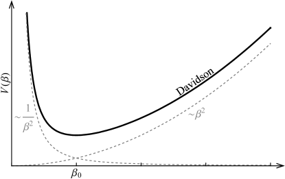
Figure 1: The $\beta$ dependence of the potential $V(\beta,\gamma)$ in (6), given by a Davidson potential in $\beta$. The minimum of the potential is at $\beta_{0}$. The asymptotic dependences $\sim\beta^{-2}$ and $\sim\beta^{2}$ are indicated by dashed lines.

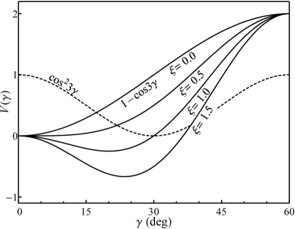
Figure 2: $\gamma$ potential V($\gamma$). The $\gamma$ dependence of the potential $V(\beta,\gamma)$ in (6), for various $\xi$, showing the dependence of the position of the minimum on $\xi$, for fixed $\chi=1$ (solid lines). The shape of the contribution from $\cos^{2}3\gamma$ is also shown (dotted line). Figure from Ref. collectiveH .

The collective Hamiltonian as formulated in (2)–(6) has five parameter degrees of freedom $(B,V_{0},\beta_{0},\chi,\xi)$. However, two of these degrees of freedom may be eliminated by use of analytic scaling relations caprio2003:gcm : (1) A simultaneous change in $B$ and $V_{0}$ of the form $V_{0}\rightarrow aV_{0}$ and $B\rightarrow a^{-1}B$, simply multiplies the Hamiltonian by an overall factor. This rescales all eigenvalues ($E\rightarrow aE$), while preserving ratios of (excitation) energies. The wave functions and thus electromagnetic matrix elements are left unchanged. (2) A simultaneous change in $V_{0}$ and $\beta_{0}$ of the form $\beta_{0}\rightarrow a^{-1}\beta_{0}$ and $V_{0}\rightarrow a^{4}V_{0}$ is recognized to yield a dilation transformation of the type defined in (5) of Ref. caprio2003:gcm . This again preserves ratios of energies, but dilates all wave functions in $\beta$, thereby introducing an overall scale factor ($\propto\beta_{0}^{2}$) to all $E2$ matrix elements. The energy and $\beta$ scales may be chosen so as to obtain any desired values for the observables $E(2^{+})$ and $\langle 2\|Q\|0\rangle$.

We are thus left with three remainining parameter degrees of freedom, which may be taken as the potential parameters $(\beta_{0},\chi,\xi)$ in (6). These must be explored through numerical diagonaliztion. In this work, the Schrödigner equation is solved using the algebraic collective model (ACM) ACM ; ACM2 , an algebraic framework for numerically solving the collective model eigenproblem in an $\mathrm{SU}(1,1)\times\mathrm{SO}(5)$ basis. The energies of the lowest collective quadrupole excitations of the adjacent even-even nucleus are used to determine these remaining parameters in the collective Hamiltonian for the core.

In particular, the collective model parameters are chosen through a least-squares fitting procedure so as to reproduce the ratios $E(2_{2}^{+})/E(2_{1}^{+})$, $E(4_{1}^{+})/E(2_{1}^{+})$, and $E(0_{2}^{+})/E(2_{1}^{+})$, together with the staggering of the quasi-$\gamma$ band, as measured by the parameter $S(R)$ defined below in (8). The staggering of the quasi-$\gamma$ band is the clearest signature to distinguish between a $\gamma$-soft or a $\gamma$-rigid nuclear shape. For example $S(4)=1.67$ for a $\gamma$ rigid triaxial rotor, and $S(4)=-2$ for a $\gamma$ independent potential stagger . The ratios $E(2_{2}^{+})/E(2_{1}^{+})$, $E(4_{1}^{+})/E(2_{1}^{+})$, $E(0_{2}^{+})/E(2_{1}^{+})$ Casten sensitively depend on all three parameters the collective potential (6) (see Ref. collectiveH ). Through manipulating the weights of the input data of the fit, parameter sets are found which in our view best account for the experimental spectra. They are listed in Table 1. The ACM solutions with these parameters provide the relative excitation energies $E(R)/E(2^{+})$ and the relative reduced matrix elements of the quadrupole operator $\langle R\|Q\|R^{\prime}\rangle/Q_{0}$, which are inputs to the CQPC model. The scales $E(2^{+})$ and $Q_{0}$ are treated as free parameters, the choice of which is discussed below in Sec. II.4.

Table 1: Parameters of the soft-core calculations, where $\left(\beta_{0},\chi,\xi\right)$ define the Davidson potential, $\kappa$ is the coupling strength of the quadrupole interaction, $E_{2}$ is the energy of the first $2^{+}$ state of the cores, and $\varepsilon_{j}-\lambda$ is the Fermi level relative to the neutron $h_{11/2}$ and the proton $g_{9/2}$ levels.

Nucleus	$\beta_{0}$	$\chi$	$\xi$	$\kappa$	$E_{2}$	$\lambda-\varepsilon_{j}$
101Pd	1.5	1.4	1	8.6	0.556	-3.487
103Pd	1.8	1.6	2.6	9.11	0.556	-2.96
105Pd	1.8	2.2	2.8	9.92	0.512	-2.47
107Pd	2.1	0.6	3	10.46	0.434	-2.028
109Pd	2.1	0.7	4	11	0.47	-1.58
111Pd	2.6	0.5	3.1	9.36	0.425	-1.0482
113Pd	2.7	0.9	3.6	7	0.419	-0.62
115Pd	2.4	0.9	3.8	8.7	0.426	-0.184
101Rh	1.5	1.4	1.1	8.6	0.556	0.61
103Rh	1.8	1.6	2.6	9.11	0.556	0.63
105Rh	1.8	2.2	2.8	9.92	0.512	0.716
107Rh	2.1	0.6	3	10.46	0.434	0.76
109Rh	2.1	0.7	4	11	0.47	0.847
111Rh	2.6	0.5	3.1	9.36	0.48	0.697
113Rh	2.7	0.9	3.6	7	0.459	0.492
115Rh	2.4	0.9	3.8	8.7	0.464	0.641
107Ru	6.5	0.3	2.5	12.57	0.242	-1.648
109Ru	2.8	1.6	1.9	12.6	0.241	-1.084
111Ru	8	0.1	2.1	13.01	0.237	-0.713
113Ru	2	2.8	1.3	13.1	0.265	0.063

Table 2: Parameters of the rigid core calculations, where $\gamma$ is the triaxiality parameter, $\kappa$ is the coupling strength of the quadrupole interaction, $E_{2}$ is the energy of the first $2^{+}$ state of the cores, and $\varepsilon_{j}-\lambda$ is the Fermi level relative to the neutron $h_{11/2}$ and the proton $g_{9/2}$ levels.

Nucleus	$\gamma$	c	$\kappa$	$E_{2}$	$\lambda-\varepsilon_{j}$
101Pd	30	0.07	8.6	0.556	-3.487
103Pd	30	0.07	9.11	0.556	-2.96
105Pd	30	0.07	9.92	0.512	-2.47
107Pd	30	0.07	10.46	0.434	-2.028
109Pd	30	0.09	11	0.44	-1.58
111Pd	30	0.07	9.36	0.433	-1.0482
113Pd	30	0.07	7	0.415	-0.62
115Pd	30	0.07	8.7	0.475	-0.184
101Rh	10	0.09	8.6	0.5	0.61
103Rh	15	0.09	9.11	0.556	0.63
105Rh	10	0.07	9.92	0.44	0.716
107Rh	10	0.07	10.46	0.434	0.76
109Rh	14	0.09	11	0.34	0.847
111Rh	14	0.07	9.36	0.349	0.697
113Rh	11	0.09	7	0.33	0.492
115Rh	11	0.08	8.7	0.34	0.641
107Ru	30	0.09	12.57	0.4	-1.648
109Ru	44	0.09	12.6	0.4	-1.084
111Ru	44	0.09	13.01	0.4	-0.713
113Ru	17	0.09	13.1	0.3	0.063

II.2 Rigid core

For the rigid triaxial core, only the triaxial rotor Hamiltonian (4) is taken into account. The triaxiality parameter $\gamma$ is fixed and adjusted as specified below. The MoI are taken to have irrotational flow dependence (5) on $\gamma$ and a scale which increases with core angular momentum $R$ as

$$\mathcal{J}_{k}^{\prime}(R)=\Theta(1+cR)\sin(\gamma-\frac{2}{3}\pi k)^{2}.$$ (7)

The parametrization $\Theta(1+cR)$ for the scale factor is motivated by the study of tidal waves in Ref. FGS11 (see also Ref. background ). There are two effects taken into account this way. The Coriolis force acts on both spins of a pair of nucleons with angular momenta in opposite directions, trying to align nucleons to the rotational axis as the total angular momentum $R$ increases, which causes a reduction of the pair correlations and an increase of the MoI peter . A second effect is a stretching of the nucleus in the $\beta$ direction with increasing $R$ for a potential with finite rigidness. The MoI of the Bohr Hamiltonian kinetic energy (5) is proportional to $\beta^{2}$. Thus, the simple relationship (7) between $\mathcal{J}^{\prime}_{i}$ and $R$ is expected background .

Thus, the triaxial rotor core is not a “rigid” rotor in the literal sense. The excitation energies of the core decrease with $(1+cR)$, which will influence the coupling between core and quasiparticle. To keep terminology simple, we will refer, somewhat loosly, to this triaxial rotor as the “rigid” core and to the collective model with the triaxial Davidson potential as the “soft” core. The parameters of the rigid core are listed in Table 2, where $\Theta$ is fixed by the energy $E(2^{+}_{1})$ of the core. The excitation energies $E_{c}(R)$ and $\langle Rk\|Q\|R^{\prime}k^{\prime}\rangle$ of the core are calculated by numerical diagonalization of the triaxial rotor Hamiltonian (4).

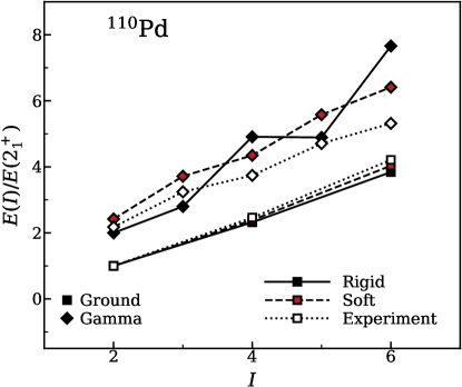
Figure 3: Ground and $\gamma$ band of the soft collective model and rigid rotor core in comparison with experiment ¹¹⁰Pd. The soft core represents a typical fit of the collective model with triaxial Davidson potential to the experiment (cf. Table 1 for parameters), which is used in the QTD calculations. The rigid rotor core is used in the QTR calculations (cf. Table 2 for parameters).

II.3 Staggering of the $\gamma$ band

A sensitive indicator of the rigidity of the collective core is the energy staggering of the $\gamma$ band, which is defined as stagger

$$S(R)=\frac{E(R)-2E(R-1)+E(R-2)}{E(2_{1}^{+})},$$ (8)

where the $E(R)$ are the energies for spin $R$ in the $\gamma$ band, and $E(2_{1}^{+})$ is the energy of the first $2^{+}$ state in the ground band. For a $\gamma$-soft core, the energies of the even-$R$ levels lie below the average of the adjacent odd-$R$ levels. For the $\gamma$-rigid core, the energies of the odd-$R$ levels lie below the average of the adjacent even-$R$ levels staggeringOddandEven .

Fig. 3 shows the ground band and $\gamma$ band of ¹¹⁰Pd as an example for a core. The ground band of the collective model core and the rigid core are close to experiment, while the $\gamma$ band of the rigid rotor has opposite staggering compared to both experiment and the collective model core.

II.4 Core-Quasiparticle Coupling Model

In the present work we use the core-quasiparticle coupling (CQPC) model cqpc . CQPC generalizes the familiar concept of BCS quasiparticles in a statically deformed potential by introducing an extended set which consists of a multitude of quasiparticle sets, each of which belongs to a potential with a different shape, where appropriate deformation parameters cover the range of the collective motion of the core. The pair field is assumed to be independent of the shape of the core. The quasiparticle are coupled by the kinetic energy operator of the collective core motion.

The CQPC model is formulated as an eigenvalue problem in the vector space where a particle is coupled to a collective states of the $A-1$ neighbor as $c^{+}_{j,m}|RM_{R}kA-1\rangle$ and a hole is coupled to the collective states of the $A+1$ neighbor as $c^{-}_{j,m}|RM_{R}kA+1\rangle$. Here, $R$ is the angular momentum of the core, $M_{R}$ is its projection and k summarizes all the remaining quantum numbers of the collective states of the core.

The Hamiltonian for the odd-mass nucleus is given by

$$H=H_{af}+H_{c},$$ (9)

where $H$ is a matrix in the above defined vector space. The matrix $H_{af}$ (adiabatic field) couples the particle and the hole to the instantaneous deformed potential and pair field, and the matrix $H_{c}$ describes the collective motion of the even-even core. The eigenvalues $E_{I}$ and the eigenvectors $\overrightarrow{uv_{I}}$ are found by diagonalizing the matrix $H$:

$$H\overrightarrow{uv_{I}}=E_{I}\overrightarrow{uv_{I}}.$$ (10)

The eigenvalues of this Hamiltonian are the excitation energies of the odd-$A$ nucleus. The eigenvectors are

$$\overrightarrow{uv_{I}}=\begin{bmatrix}\overrightarrow{u_{I}}\\ \overrightarrow{v_{I}}\end{bmatrix}=\begin{bmatrix}\langle RM_{R}kA-1|c_{jm}|IMA\rangle\\ \langle RM_{R}kA+1|c^{+}_{j\bar{m}}|IMA\rangle\end{bmatrix},$$ (11)

where $\overrightarrow{u_{I}}$ represents the probability amplitude for the considered states $|IMA\rangle$ of the odd-$A$ nucleus composed of a particle in the (A-1) nucleus, and $\overrightarrow{v_{I}}$ represents the probability amplitude for a hole in the (A+1) nucleus. Here, jm are the quantum numbers of the particle and hole within a major shell, $RM_{R}k$ are the quantum numbers of the collective states of the even-even core, and $IM$ are the angular momentum and its projection of the odd mass nucleus. Note, the square of the amplitudes are the spectroscopic factors for particle transfer reactions.

The Hamiltonian of the odd quasiparticle reads

$$H_{af}=\begin{bmatrix}\varepsilon-\lambda+\tau&\Delta\\ \Delta&-(\varepsilon-\lambda+\tau)\end{bmatrix},$$ (12)

and the Hamiltonian of the even-even core

$$H_{c}=\begin{bmatrix}E_{c}&0\\ 0&E_{c}\end{bmatrix}.$$ (13)

In these equations, $\varepsilon_{j}$ is the energy of the spherical $j$-shell, $\lambda$ is the chemical potential, $\Delta$ is the pairing field, and $E_{c}$ are the energies of the core collective quadrupole excitations.

The interaction $\tau$ between the particle and the core is described by the quadrupole field, which can be expressed as:

$$(\tau)_{jRk,j^{\prime}R^{\prime}k^{\prime}} = -\frac{\kappa}{2}(-1)^{j^{\prime}+R^{\prime}+I}\begin{Bmatrix}j&j^{\prime}&2\\ R&R^{\prime}&I\end{Bmatrix}$$ (14)

$$\times\langle Rk\|Q\|R^{\prime}k^{\prime}\rangle q_{jj^{\prime}},$$

where $\langle Rk\|Q\|R^{\prime}k^{\prime}\rangle$ and $q_{jj^{\prime}}$ are the quadrupole reduced matrix elements of the core and particle, and $\kappa$ is the coupling strength of the quadrupole field. The quantum numbers of the even-even core are $R$, $k$, $R^{\prime}$, $k^{\prime}$, and $j$, $j^{\prime}$ are quantum numbers of the particle. The $M_{R}$ and $m$ dependence is taken care of by angular momentum algebra, which leads to the reduced matrix elements cqpc .

In the general application of the QPCM the spherical single particle energies $\varepsilon_{j}$ are taken from a spherical potential, as the Nilsson or Woods-Saxon potential or some more sophisticated energy density functional (EDF) approach. In the present paper only the coupling of the $h_{11/2}$ quasineutrons and the $g_{9/2}$ quasiprotons is studied. For them one can set $\varepsilon_{j}=0$, without loss of generality. The pairing gap $\Delta$ is set to 1.226 MeV.

The coupling strength of the quadrupole interaction $\kappa$ is evaluated using the self-consistency condition for the QQ-model

$$\kappa/5=\hbar w_{0}\bar{\beta}\langle 2\|Q\|0\rangle,$$ (15)

where $\hbar w_{0}=41A^{-1/3}$MeV, and the scale $Q_{0}$ of the core matrix elements is chosen such that $\langle 2\|Q\|0\rangle=1$. The core deformation $\bar{\beta}$ is taken from the compilation raman , which relates $\bar{\beta}$ to the experimental $B(E2;0\rightarrow 2)$ by

$$\bar{\beta}=\left[\frac{4\pi Ze^{2}R_{0}^{2}}{3B(E2;0\rightarrow 2)}\right]^{1/2}.$$ (16)

The resulting coupling constants $\kappa$ are listed in Tables 1 and 2.

The particle number n for the state $|IMA\rangle$ is given by

$$n=\sum_{jmkRM_{R}}|\langle IMA|c^{+}_{jm}|RM_{R}kA-1\rangle|^{2}.$$ (17)

As usual in BCS, the chemical potential $\lambda$ is determined by the condition $n=A$. In practice, it is fixed for the ground state of the odd nucleus and kept constant for the other states. In this paper we only study the coupling to the $h_{11/2}$ neutron and the $g_{9/2}$ protons, which are approximated as pure $j$-shells. In the calculations $\lambda-\varepsilon_{j}$ is needed, which is also listed in the tables. All single particle energies $\varepsilon_{j}$ within the major shell are needed to obtain the particle number (17), which are taken from the Nilsson potential.

II.5 Wobbling motion of triaxial nuclei

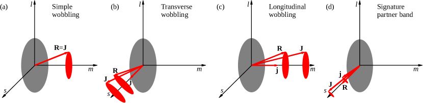
Figure 4: Different types of wobbling motion. The four panels correspond to (a) simple wobbbling, (b) transverse wobbling, (c) longitudinal wobbling, and (d) the signature partner band. Here $l$, $m$ and $s$ indicate the long, medium and short axes, respectively, with corresponding MoI ordered as $\mathcal{J}_{m}>\mathcal{J}_{s}>\mathcal{J}_{l}$. The arrows represent the angular momentum $\boldsymbol{\mathbf{\mathrm{R}}}$ of the core, the angular momentum $\boldsymbol{\mathbf{\mathrm{j}}}$ of the quasiparticle, and the total angular momentum $\boldsymbol{\mathbf{\mathrm{J}}}$.

The coupling of an odd quasiparticle to a rigid triaxial rotor has been classified in Ref. transverse . This classification is summarized in Fig. 4, where the axes represent the medium ($m$), short ($s$), and long ($l$) body-fixed axes of the nucleus. The MoI are assumed to be ordered as $\mathcal{J}_{m}>\mathcal{J}_{s}>\mathcal{J}_{l}$ for these axes, respectively.

The wobbling motion of the triaxial rotor itself, without an odd quasiparticle, has been discussed by Bohr and Mottelson BohrMottlelsonII . It is illustrated in Fig. 4(a), where, following Ref. transverse , such wobbling is termed “simple wobbling”. In classical mechanics, uniform rotation around the axis with the largest MoI (here, the $m$-axis) has minimal energy for given angular momentum. At larger energy, rotation about the other two axes appears, which generates a wobbling of the triaxial body with respect to the space-fixed angular momentum vector. In the body-fixed frame, the wobbling motion represents a precession of the angular momentum vector around the axis with the largest MoI (again, here, the $m$-axis).

In the small-amplitude limit, such motion has a quantized energy spectrum given by:

$$\textit{E}(n_{w},I)=\frac{\hbar^{2}}{2\mathcal{J}_{m}}I(I+1)+(n_{w}+1/2)\hbar\omega_{w},$$ (18)

where $n_{w}$ describes the wobbling phonon number and $I$ is the total angular momentum transverse . The wobbling frequency $\omega_{w}$ is determined by

$$\hbar\omega_{w}=\frac{I\hbar^{2}}{\mathcal{J}_{m}}\sqrt{\left(\frac{\mathcal{J}_{m}}{\mathcal{J}_{s}}-1\right)\left(\frac{\mathcal{J}_{m}}{\mathcal{J}_{l}}-1\right)}.$$ (19)

It is to be compared with the experimental wobbling energy $\textit{E}_{w}$ defined as transverse :

$$\textit{E}_{w}(I) = \textit{E}(n_{w}=1,I)$$

$$-[\textit{E}(n_{w}=0,I-1)+\textit{E}(n_{w}=0,I+1)]/2,$$

For an even-even triaxial nucleus or “simple wobbler”, the wobbling energy increases with $I$.

The wobbling motion is modified for odd-mass nuclei, as discussed in Ref. transverse . Fig. 4(b) illustrates the case where there is a high-$j$ quasiparticle coupled to the core. The quasiparticle’s angular momentum $j$ aligns with the $s$-axis (with intermediate MoI), which is transverse to the $m$-axis (with the maximal MoI). The wobbling motion consists in the precession of the angular momentum vector about the transverse $s$-axis and is thus termed “transverse wobbling” transverse . In the harmonic approximation, the energy of the wobbling bands is given by

$$\textit{E}(n_{w},I)=\frac{\hbar^{2}}{2\mathcal{J}_{s}}(I+1/2-j)^{2}+(n_{w}+1/2)\hbar\omega_{w},$$ (21)

with the wobbling frequency

$$\hbar\omega_{w}=\frac{I\hbar^{2}}{\mathcal{J}_{s}}\sqrt{\left(\frac{\mathcal{J}_{s}}{\mathcal{J}_{m}}-1+\frac{j}{I}\right)\left(\frac{\mathcal{J}_{s}}{\mathcal{J}_{l}}-1+\frac{j}{I}\right)}.$$ (22)

As $\mathcal{J}_{s}/\mathcal{J}_{m}<1$, the first factor $({\mathcal{J}_{s}}/{\mathcal{J}_{m}}-1+{j}/{I})$ inside the radical decreases with $I$, until it crosses zero, while, as $\mathcal{J}_{s}/\mathcal{J}_{l}>1$, the second factor $({\mathcal{J}_{s}}/{\mathcal{J}_{l}}-1+{j}/{I})$ monotonically decreases. Consequently, considering the effects of all factors together, the wobbling frequency $\hbar\omega_{w}$ first briefly increases with $I$, then decreases with $I$, until it vanishes at the critical angular momentum

$$I_{c}=\frac{j\mathcal{J}_{m}}{\mathcal{J}_{m}-\mathcal{J}_{s}},$$ (23)

at which point the transverse wobbling mode becomes unstable. This is to be contrasted with the simple wobbler above, for which the wobbling frequency (19) simply increases linearly with $I$.

The case when the angular momentum $j$ of the quasiparticle is aligned with the $m$-axis, which appears for a quasiparticle in a half-filled $j$-shell, is illustrated in Fig. 4(c). The wobbling motion then consists in the precession of the angular momentum vector about the $m$-axis (with the maximal MoI) and is thus termed “longitudinal wobbling” transverse . In the harmonic approximation, the energy of the wobbling bands is given by

$$\textit{E}(n_{w},I)=\frac{\hbar^{2}}{2\mathcal{J}_{m}}(I+1/2-j)^{2}+(n_{w}+1/2)\hbar\omega_{w},$$ (24)

with the wobbling frequency

$$\hbar\omega_{w}=\frac{I\hbar^{2}}{\mathcal{J}_{m}}\sqrt{\left(\frac{\mathcal{J}_{m}}{\mathcal{J}_{s}}-1+\frac{j}{I}\right)\left(\frac{\mathcal{J}_{m}}{\mathcal{J}_{l}}-1+\frac{j}{I}\right)}.$$ (25)

As $\mathcal{J}_{m}/\mathcal{J}_{s}>1$ and $\mathcal{J}_{m}/\mathcal{J}_{l}>1$, both factors within the radical decrease with $I$. This has the consequence that, although the frequency $\hbar w_{w}$ of longitudinal wobbling increases with $I$, it does so less rapidly than for the simple wobbler (19).

In the following we call the lowest-energy band with $n_{w}=0$ the “yrast band”, and we call the one-phonon ($n_{w}=1$) excited band on top of the yrast band the “wobbling band”. Because of the $D_{2}$-symmetry of the triaxial potential the bands have good signature $\alpha=\pm 1/2$. They form $\Delta I=2$ sequences with $I=1/2,5/2,9/2,\ldots$ for $\alpha=+1/2$ or $I=3/2,7/2,11/2,\ldots$ for $\alpha=-1/2$. For the considered case of $h_{11/2}$ quasiparticles, the yrast band has $\alpha=-1/2$, and the wobbling band has $\alpha=+1/2$.

There is another $\alpha=+1/2$ band, which we call the “signature partner” band. The signature partner for the case of transverse coupling of the quasiparticle is illustrated in Fig. 4(d). For the signature partner band, the angular momentum of the quasiparticle is no longer maximally aligned ($m=j$) with the $s$-axis, but it precesses around the $s$-axis with $m=j-1$, where the collective angular momentum is aligned with the $s$-axis. Signature partner bands are well known from the classification of rotational spectra in terms of quasiparticles in a rotating potential peter .

As an example, Fig. 5(b) below (in Sec. III), shows the three lowest bands in ¹⁰⁹Pd obtained by the QTR calculation that couples a $h_{11/2}$ quasineutron to a triaxial rotor with $\gamma=30^{\circ}$. The lowest band, which we refer to as yrast in the following, has $\alpha=-1/2$. The two excited bands have $\alpha=1/2$.

The probabilities for the $\Delta I=1$ transitions to the yrast band clearly distinguish the wobbling band from the signature partner band. As seen in Fig. 5(d), the $B(E2)$ values of the transitions from the band that we classify as wobbling are much larger than those from the signature partner band. As illustrated in Fig. 4(b), the precession of the total angular momentum vector $\boldsymbol{\mathbf{\mathrm{J}}}$ about the $s$-axis of the body fixed frame means that the triaxial charge distribution wobbles in the laboratory system, which generates collectively enhanced $E2$ radiation. By analyzing the wave functions of the odd-mass nuclei, we found that for the same total $J$, the core angular momentum $\boldsymbol{\mathbf{\mathrm{R}}}_{\perp}$ of the wobbling band is large. This is because transverse wobbling approaches instability with respect to a permanent tilt of the rotational axis relative to the $s$-axis. The cases with longitudinal wobbling character have been found to have a large wobbling amplitude as well.

To discuss the signature partner band it is noted that the total angular momentum is expressed as $\boldsymbol{\mathbf{\mathrm{J}}}=\boldsymbol{\mathbf{\mathrm{j}}}+\boldsymbol{\mathbf{\mathrm{R}}}$, and its transverse component relative to the total angular momentum $\boldsymbol{\mathbf{\mathrm{J}}}_{\perp}=0$ by definition, which gives $\boldsymbol{\mathbf{\mathrm{R}}}_{\perp}=-\boldsymbol{\mathbf{\mathrm{j}}}_{\perp}$. As illustrated in Fig. 4(d), the quasiparticle is no longer aligned with the $s$-axis, but precesses around it with $j_{\perp}=\sqrt{2j}\approx 2$. The associated precession of $\boldsymbol{\mathbf{\mathrm{J}}}$ corresponds to much weaker oscillations of the charge quadrupole moment than the large-amplitude precession of $\boldsymbol{\mathbf{\mathrm{J}}}$ of the wobbling band. The oscillations of the quadrupole moment generate the $E2$ radiation, where $B(E2)$ is proportional to the squared amplitude of these oscillations transverse , which explains the large difference between the $B(E2)$ values.

Fig. 5(e) shows that the $B(M1)$ values of the transitions from band that we classify as wobbling are much larger than those from the signature band. The oscillations of the magnetic moment generate the $M1$ radiation, where $B(M1)$ is proportional to the squared amplitude of these oscillations transverse . The magnetic moment is given by

$$\boldsymbol{\mathbf{\mathrm{\mu}}}_{\mathrm{total}}=\boldsymbol{\mathbf{\mathrm{\mu}}}_{\mathrm{particle}}+\boldsymbol{\mathbf{\mathrm{\mu}}}_{\mathrm{core}},$$ (26)

with

$$\boldsymbol{\mathbf{\mathrm{\mu}}}_{\mathrm{particle}}=g_{j}\boldsymbol{\mathbf{\mathrm{j}}}\quad\boldsymbol{\mathbf{\mathrm{\mu}}}_{\mathrm{core}}=g_{R}\boldsymbol{\mathbf{\mathrm{R}}},$$ (27)

where $g_{j}$ and $g_{R}$ are the single-particle and core $g$ factors, respectively. As the vectors $\boldsymbol{\mathbf{\mathrm{j}}}$ and $\boldsymbol{\mathbf{\mathrm{R}}}$ precess about the constant total angular momentum $\boldsymbol{\mathbf{\mathrm{J}}}$, only $\boldsymbol{\mathbf{\mathrm{R}}}_{\perp}$ and $\boldsymbol{\mathbf{\mathrm{j}}}_{\perp}$ are time dependent. The transverse component of the total magnetic moment can be therefore written in either of two ways:

$$\boldsymbol{\mathbf{\mathrm{\mu}}}_{\perp} =\boldsymbol{\mathbf{\mathrm{j}}}_{\perp}(g_{j}-g_{R})$$ (28)

$$\boldsymbol{\mathbf{\mathrm{\mu}}}_{\perp} =\boldsymbol{\mathbf{\mathrm{R}}}_{\perp}(g_{R}-g_{j}).$$ (29)

The geometry of the transverse wobbling band is illustrated in Fig. 4(b). Since the quasiparticle is aligned with $s$-axis when the $M1$ transitions from the wobbling band to the yrast band are considered, we use the expression (29) to describe the transverse magnetic moment. As discussed for the $E2$ transitions, $\boldsymbol{\mathbf{\mathrm{R}}}_{\perp}$ of the wobbling band is large, because transverse wobbling approaches instability with respect to a permanent tilt of the rotational axis relative to the $s$-axis.

For the magnetic transitions from the signature partner to the yrast band we use expression (28). As illustrated in Fig. 4(d) and discussed for the $E2$ transition, the quasiparticle precesses around the m-axis, with $j_{\perp}=\sqrt{2j}\approx 2$, which is much smaller than $R_{\perp}$ for the wobbling band. Accordingly, the $B(M1)$ of the transition from the wobbling band to the yrast band is much bigger than that of the transition from the signature partner band to the yrast band.

III Discussion

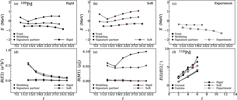
Figure 5: Comparison between QTR (rigid core) and QTD (soft core) predictions, along with experiment, for ¹⁰⁹Pd: (a-c) Energies, minus a rotor contribution, within the yrast band (squares), wobbling band (triangles), and signature partner band (circles). (d-e) Transition $B(E2)$ and $B(M1)$ strengths from the wobbling band (triangles) and signature partner band (circles) to the yrast band. (f) Normalized energies within the ground band (squares) and $\gamma$ band (diamonds) for the ¹¹⁰Pd core. Observables are shown vs. $I$, for rigid calculations (solid symbols, solid lines), soft calculations (red shaded symbols, dashed lines), and experiment (open symbols, dotted lines).

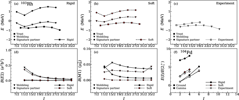
Figure 6: Comparison between QTR (rigid core) predictions, QTD (soft core) predictions, and experiment for ¹⁰³Rh, along with normalized energies for the ¹⁰⁴Pd core. See Fig. 5 caption for description of observables and notation.

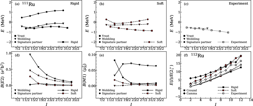
Figure 7: Comparison between QTR (rigid core) predictions, QTD (soft core) predictions, and experiment for ¹¹¹Ru, along with normalized energies for the ¹¹²Ru core. See Fig. 5 caption for description of observables and notation.

The purpose of this paper is to compare the coupling of a quasiparticle to the collective model core with soft triaxial potential, through quasipartical triaxial Davidson (QTD) calculations which take fluctuation of the triaxial shape explicitly into account, and quasiparticle triaxial rotor (QTR) calculations, which do not do so. The consequences of triaxiality for an odd-mass nucleus will be studied by comparing the two different approaches as follows. In the QTR calculations the $\gamma$ parameter of the TR is adjusted such that the calculated wobbling energy of odd-mass nucleus is obtained as close as possible to the experimental wobbling energy. In the QTD calculations, the properties of even-even nuclei are fixed first with experimental bands energies, then a quasiparticle is coupled to the core to describe odd mass nuclei. The model parameters used for calculating properties of ^109-115Pd, ^109-115Rh and ^107-113Ru are listed in Table 1 for the soft core and in Table 2 for the hard core.

Fig. 5(a)-(c) show the experimental and calculated (QTR and QTD) level energies for yrast, wobbling and signature partner bands in ¹⁰⁹Pd. For $N=63$ the occupation of the $h_{11/2}$ shell is about 3. Accordingly, Fig. 5(a) shows that the QTR starts with a decreasing wobbling energy as a function of angular momentum. This transverse wobbling regime quickly becomes unstable and changes into the longitudinal wobbling regime with increasing wobbling energy (see discussion of the stability of the transverse wobbling regime in Ref. Chen22 ). The QTD calculation in Fig. 5(b) shows a steady increase of the wobbling energy with $I$, which signals the longitudinal wobbling regime. The fluctuations of $\gamma$ toward axial shape further weaken the already weak transverse coupling of the quasineutron, which results in longitudinal wobbling wobbling right from the lowest values of $I$. This is consistent with the steady increase seen in experiment in Fig. 5(c) and the missing staggering of the $\gamma$ band of ¹¹⁰Pd in Fig. 5(f).

Fig. 5(d) and (e) compare the electromagnetic ($E2$ and $M1$) reduced transition probabilities. The $B(E2)$ values are quite similar between the approaches, whereas the $B(M1)$ values of QTR for the transitions from wobbling to yrast band are higher than those of QTD. Fig. 5(f) shows the energy ratios vs. $I$ of the ground band and $\gamma$ band of the core ¹¹⁰Pd for the experiment, collective model and triaxial rotor. The TD core, which is fitted to experimental energies, reproduces the “even-$I$-low pattern” of the quasi-$\gamma$ band (the energies of even angular momentum states are lower than that average of their odd angular momentum neighbors), which is observed in ¹¹⁰Pd. The TR core parameters are adjusted to the experimental wobbling band energies of ¹⁰⁹Pd. The inherent assumption of stable triaxiality is reflected by the characteristic “odd-$I$-low pattern” (the energies of odd angular momentum states are lower that that average of their even angular momentum neighbors) of the quasi-$\gamma$ band of the core background .

Fig. 6 provides the same information for ¹⁰³Rh, which has a quasi-proton coupled to ¹⁰⁴Pd. The proton number in the $g_{9/2}$ shell is around 6, which means the shell is about half-occupied. Accordingly, the wobbling energy increases with $I$, where there is no qualitative difference between the soft and rigid cores. Longitudinal wobbling appears for a quasiparticle in a half-filled shell, which is longitudinally coupled.

Fig. 7 shows ¹¹¹Ru which has a quasi-neutron coupled to ¹¹²Ru. For $N=68$ the $h_{11/2}$ shell is half-occupied. Accordingly, the quasineutron is longitudinally coupled to the triaxial core, which in the QTR calculation gives an increase in wobbling energy with $I$ that signals longitudinal wobbling. The QTD calculation gives quite similar results, which is expected because the TD core fitted to the experiment comes close to the TR core [see Fig. 7(f)].

The examples in Figs. 5, 6, 7 demonstrate that including softness by means of the phenomenological core like the TD always leads to the longitudinal wobbling pattern of wobbling energy increasing with $I$. Only if the quasiparticle has particle-like character (¹⁰⁹Pd) the rigid TR core generates the transient transverse wobbling pattern, the presence or absence of chich can be taken as a qualitative measure of the core’s softness.

The $B(M1)$ values for transitions from the wobbling to the yrast band are a more sensitive way to differentiate between the QTR and QTD calculations. The difference can be explained as follows. The coupling between the quasiparticle and the core is not rigid. Therefore, the total magnetic moment does not rigorously follow the motion of the core. The strength of the coupling between the quasiparticle and core will influence the amplitude of the oscillations of the magnetic moment. When the core includes $\beta$- and $\gamma$-vibrational motion, these fluctuations will reduce the coupling strength between the quasiparticle and the core. This is in contrast to the rigid TR core, which has only rotational motion. This explains why the $B(M1)$ of the transitions from the wobbling to the yrast band are bigger in the QTR calculations than in the QTD calculations.

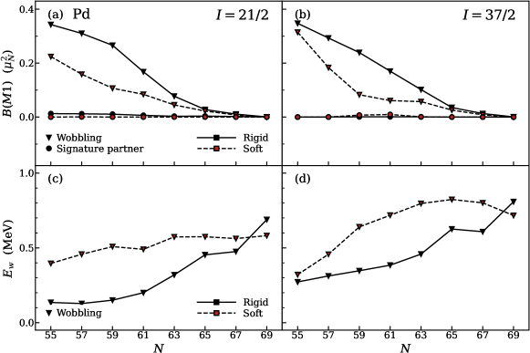
Figure 8: Comparison between QTR (rigid core) predictions and QTD (soft core) predictions for the Pd isotopic chain: (top) $B(M1)$ strength and (bottom) wobbling energy $E_{w}$, at fixed angular momenta $I=21/2$ (left) and $I=37/2$ (right). Observables are shown for rigid calculations (solid symbols, solid lines) and soft calculations (red shaded symbols, dashed lines), and for the wobbling band (triangles) and (in the case of the $M1$ strength) signature partner band (circles). The $M1$ transition is for angular momenta $I\rightarrow(I-1)$, from the wobbling or signature partner band to the yrast band.

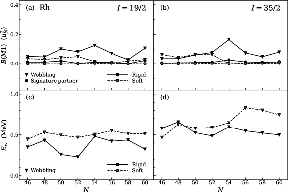
Figure 9: Comparison between QTR (rigid core) predictions and QTD (soft core) predictions for the Rh isotopic chain: (top) $B(M1)$ strength and (bottom) wobbling energy $E_{w}$, at fixed angular momenta $I=19/2$ (left) and $I=35/2$ (right). See Fig. 8 caption for description of observables and notation.

Figure 10: Comparison between QTR (rigid core) predictions and QTD (soft core) predictions for the Ru isotopic chain: (top) $B(M1)$ strength and (bottom) wobbling energy $E_{w}$, at fixed angular momenta $I=21/2$ (left) and $I=37/2$ (right). See Fig. 8 caption for description of observables and notation.

Figs. 8, 9, 10 compare QTR with QTD calculations for the Pd, Rh, and Ru isoptopes, respectively. Only the results for two selected values of $I$ are shown. More detailed results can be found in Ref. thesisLi .

Fig. 8 shows the Pd chain. For $I=21/2$ it can be seen that $B(M1)$ values for the transition from the wobbling to the yrast band decrease as the neutron number increases, while the wobbling energies increase. This is explained by the number of particles located in the $h_{11/2}$ shell, which increases from 0.62 to 5.6 (half-occupied $h_{11/2}$ shell). So the quasiparticle character changes half-way from particle-like towards hole-like as the particle number in the $h_{11/2}$ shell increases. For the rigid TR core this means the following. When the quasi-particle has a particle character, its angular momentum aligns with the $s$-axis of the TR core, since in this way the density distribution of the particle has the maximal overlap with core the density distribution. When the quasi-particle has hole character, its angular momentum aligns with the $l$-axis of the TR core, because for this orientation the density distribution of the hole has minimal overlap with the core density distribution. When the quasiparticle’ s character is in-between particle and hole, its angular momentum tends to be aligned with the $m$-axis of the TR core. When the quasiparticle is a particle or hole, it will oscillate rigidly with the axis, giving a strong $B(M1)$. But when the quasiparticle is in-between particle and hole, it will be partially decoupled from the core, resulting in a small $B(M1)$ and a big wobbling energy. In contrast,the $E2$ radiation mostly comes from the collective core, which is why the $B(E2)$ values do not change dramatically with neutron number. For the soft TD core the fluctuations away from the triaxial shape attenuate the transverse coupling of the quasiparticle, which is seen as larger wobbling energies and smaller $B(M1)$ values. The soft core and rigid core results approach each other near $N=66$ because the TD fits approach the rigid rotor.

For $I=37/2$, the TR wobbling energies are about the same or larger than those for $I=27/2$. The detailed calculations thesisLi show that the wobbling energies first go down and then go up, like in Fig. 5, which corresponds to a short transverse wobbling phase that changes into longitudinal wobbling. The TD wobbling energies for $I=37/2$ are larger than for $I=27/2$, which signals the presence of the longitudinal wobbling regime as in Fig. 5. The $B(M1)$ values for TD are smaller than those for TR. The $I$ dependence is similar to that for $I=27/2$.

Fig. 9 presents $B(M1)$ values and wobbling energies of the isotopes ^101-115Rh. The proton number in the $g_{9/2}$ shell is constant around 6. As a consequence, the character of the quasiparticle does not change. The changes of the wobbling energies and $B(M1)$ values are caused by the $N$-dependence of the core. The dip of the QTR wobbling energy around $N=50$ may be an artifact, because modeling these nuclei as TR is not very realistic. The more realistic TD cores give a smooth $N$-dependence in the region. For $N\geq 58$ the QTR model seems acceptable. The comparison with the QTD shows the same pattern as for the odd-neutron nuclei. The QTD wobbling energies are larger than the QTR ones and the $B(M1)$ values are smaller, where the $B(M1)$ values are small overall. As seen in Fig. 6, the wobbling energies increase with $I$ indicating longitudinal wobbling. The Ru isotopes in Fig. 10 are similar to the Pd isotopes, which are discussed above.

From Figs. 8, 9 and 10, it can be seen that large strength for the $B(M1)$ transition corresponds to small wobbling energy and vice versa. Both quantities reflect the coupling strength of the quasiparticle to the triaxial core. Strong coupling enhances the $B(M1)$ values and it favours the transverse wobbling, which corresponds to small wobbling energy. For example, in the Rh chain QTR calculations the coupling depends on the $\gamma$ parameter of the TR core. When $\gamma$ $\approx$ $30^{\circ}$, the wobbling energy is not close to the experimental one, and the $B(M1)$ values of QTR calculations are smaller than those of the QTD calculations. But when $\gamma$ is adjusted to reproduce the experimental wobbling energy, the $B(M1)$ values are increased substantially, becoming larger than in the QTD calculations.

IV Summary

In this paper the triaxiality of odd-mass nuclei was explored by investigating the coupling of an odd high-$j$ quasiparticle to the triaxial core represented by the even-even neighboring nuclei. Two kinds of core models were studied. The “soft core” takes the rotation-vibrational motion of the shape into account. In this description, the core was described by a Bohr Hamiltonian with a simple few-parameter potential, which provides soft confinement both in $\beta$ and $\gamma$. In particular, we adopted a triaxial Davidson potential collectiveH , solved numerically using the Algebraic Collective (ACM) approach. The parameters were determined by fitting the energies of the lowest collective states of the even-even neighbors. The coupling of the odd quasiparticle to this soft core was then described by means of the quasiparticle-core coupling model of Ref. cqpc , resulting in a description of the odd-mass nucleus which we termed the quasiparticle triaxial Davidson (QTD) model. The resulting energies and electomagnetic transition probabilities were compared with those obtained by coupling the quasiparticle to a “rigid core” described by the simple triaxial rotor model, in what we referred to as the quasiparticle triaxial rotor (QTR) model. This represent the limiting case of the QTD model where a stiff potential for the vibrational modes leaves only the rotational motion active.

We studied the isotopic chains ^101-115Pd, ^101-115Rh, and ^107-113Ru. These examples paint a general picture. The “rigid core” QTR calculations gave for some cases the transverse wobbling pattern, where the wobbling energy decreases with angular momentum then increases after some point, but in most cases the longitudinal wobbling pattern, where the wobbling energy steadily increases with angular momentum. The competition between transverse and longitudinal wobbling depends on the coupling strength between core and quasiparticle, which is determined by the triaxiality of the core and the position within the $j$-shell (top or bottom: transverse orientation; middle: longitudinal orientation). Only a few of the QTR calculations resulted in a transverse wobbling pattern, when the triaxiality parameter of the TR was close to $30^{\circ}$ and the odd quasineuton was nearly a pure particle. The QTD calculations always gave the longitudinal wobbling pattern, even for the cases where the QTR model provided transverse wobbling. The reason is that in contrast to the rigid TR core the soft TD core takes large excursions into regions of small triaxiality.

Besides the different $I$ dependence of the energy difference, the soft core leads to weaker $B(M1)$ values for the $\Delta I=1$ transitions from the wobbling band to the yrast band. The $B(E2)$ values for the same transitions for both types of cores are collectively enhanced and not very different.

The tranverse wobbling pattern is observed experimentally. For the nuclei studied here it appears in a volatile way for ¹⁰¹Pd, and much more clearly for ¹³⁵Pr pr135 and neighboring nuclei. In all cases, only the rigid TR core is capable of accounting for the observed pattern, while the soft TD core leads to longitudinal wobbling (see Ref. thesisLi for ¹³⁵Pr). This means that the coupling of the odd particle does not sufficiently polarize the phenomenological TD core, such that the tranverse wobbling pattern of the rigid core appears. The “soft core” derived from the neighboring even-even nuclei coupled to a quasiparticle no longer describes the odd mass nucleus, which is better described by a “rigid core” coupled to a quasiparticle.

The important implication is that the presence of the quasiparticle changes the rigidity of the “core”. The CQPC model assumes that the collective degrees of freedom of the core and the quasiparticle degrees of freedom are independent. However, the collective excitations of the core are superpositions of two-, four-, $\ldots$ quasiparticle excitations. The presence of the odd quasiparticle blocks some of these quasiparticle excitations, which modifies the response of the core relative to that which is observed in the even-even neighbors.

These modifications of the core and the ensuing changes of the coupled system have been studied for spherical nuclei in the framework of nuclear field theory NFT . The Klein-Kerman (KK) equation of motion method kerman1962:eom accounts for these effects in principle. However, the anti-symmetrization between quasiparticle and core has only be taken into account for the triaxial rotor, which leads to the self-consistent triaxial rotor model. The modifications of the rotor core solved the longstanding Coriolis attenuation problem of the conventional particle rotor model (see Ref. Klein00 and references therein). For more general core models the KK approach became became a practical tool only after the introduction of the Dönau-Frauendorf approximation (DF), which neglects the core modifications terms (giving the KKDF method). The resulting CQPC formalism was used in this paper (for a discussion of the DF approximation see Refs. cqpc ; Klein04 ).

A promising new avenue is the triaxial projected shell model (TPSM) sheikh1999:tpsm . The TSPM has been demonstrated Jehangir21 to be capable of describing the energies and quadrupole matrix elements of both $\gamma$-rigid and $\gamma$-soft even-even nuclei, by diagonalizing a pairing plus quadrupole-quadrupole Hamiltonian, in a basis of states comprised of multiquasiparticle excitations in a fixed triaxial mean field, projected onto good angular momentum. The TPSM also correctly describes transverse wobbling in ¹³⁵Pr Sensharma19 . It is of interest to study neighbor ¹³⁴Ce within the framework of the TPSM in order to exemplify the core modification as a consequence of the exclusion principle for fermions. Work along these lines is in progress.

- (1) P. Möller et al., Phys. Rev. Lett. 97, 162502 (2006).
- (2) N. Zamfir and R. Casten, Phys. Lett. B 260, 265 (1991).
- (3) E. A. McCutchan, D. Bonatsos, N. V. Zamfir, and R. F. Casten, Phys. Rev. C 76, 024306 (2007).
- (4) M. A. Caprio, Phys. Rev. C 83, 064309 (2011).
- (5) S. Frauendorf, Int. J. Mod. Phys. E 24, 1541001 (2015).
- (6) J. Meyer-ter-Vehn, Nucl. Phys. A 249, 111 (1975).
- (7) H. Toki and A. Faessler, Nucl. Phys. A 253, 231 (1975).
- (8) A. Bohr and B. Mottelson Nuclear Structure: Nuclear Deformations, Vol. II (World Scientific, Singapore, 1998).
- (9) S. W. Ødegård et al., Phys. Rev. Lett. 86, 5866 (2001).
- (10) I. Hamamoto and G. B. Hagemann, Phys. Rev. C 67, 014319 (2003).
- (11) S. Frauendorf and F. Dönau, Phys. Rev. C 89, 014322 (2014).
- (12) J. T. Matta, U. Garg, W. Li, S. Frauendorf, A. D. Ayangeakaa, D. Patel, K. W. Schlax, R. Palit, S. Saha, J. Sethi, T. Trivedi, S. S. Ghugre, R. Raut, A. K. Sinha, R. V. F. Janssens, S. Zhu, M. P. Carpenter, T. Lauritsen, D. Seweryniak, C. J. Chiara, F. G. Kondev, D. J. Hartley, C. M. Petrache, S. Mukhopadhyay, D. V. Lakshmi, M. K. Raju, P. V. Madhusudhana Rao, S. K. Tandel, S. Ray, and F. Dönau, Phys. Rev. Lett. 114, 082501 (2015).
- (13) S. Frauendorf and J. Meng, Nucl. Phys. A 617, 131 (1997).
- (14) J. Meng and S. Q. Zhang, J. Phys. G 37, 064025 (2010).
- (15) S. Frauendorf and F. Dönau, Phys. Lett. B 71, 263 (1977).
- (16) J. Timár, Q. B. Chen, B. Kruzsicz, D. Sohler, I. Kuti, S. Q. Zhang, J. Meng, P. Joshi, R. Wadsworth, K. Starosta, Phys. Rev. Lett. 122, 062501 (2019).
- (17) W. C. Li, Algebraic Collective Model and Its Applications to Core Quasiparticle Coupling, Ph.D. thesis, University Notre Dame (2016), URL https://curate.nd.edu/show/6682x348f37.
- (18) J. P. Elliott, J. A. Evans, and P. Park, Phys. Lett. B 169, 309 (1986).
- (19) F. Iachello, Phys. Rev. Lett. 91, 132502 (2003).
- (20) M. A. Caprio, Phys. Lett. B 672, 396 (2009).
- (21) M. A. Caprio, Phys. Rev. C 68, 054303 (2003).
- (22) D. Rowe and P. Turner, Nucl. Phys. A 753, 94 (2005).
- (23) D. J. Rowe, T. A. Welsh, and M. A. Caprio, Phys. Rev. C 79, 054304 (2009).
- (24) R. F. Casten and N. V. Zamfir, Phys. Rev. Lett. 87, 052503 (2001).
- (25) S. Frauendorf, Y. Gu, J. Sun, Int. J. Mod. Phys. E 20, 465 (2011).
- (26) P. Ring and P. Schuck, The nuclear many-body problem. (Springer-Verlag, 1980).
- (27) S. Raman, C. W. Nestor, Jr., and P. Tikkanen, At. Data Nucl. Data Tables 78, 128 (2001).
- (28) Q. B. Chen and S. Frauendorf, Eur. Phys. J. A 58, 75 (2022).
- (29) P. F. Bortignon, R. A. Broglia, D. R. Bes, and R. Liotta, Phys. Rep. 30, 305 (1977).
- (30) A. Kerman and A. Klein, Phys. Lett. 1, 185 (1962).
- (31) A. Klein, Phys. Rev. C 63, 014316 (2000).
- (32) A. Klein, P. Protopapas, S. G., Rohoziǹski, and K. Starosta, Phys. Rev. C 69, 034338 (2004).
- (33) J. A. Sheikh and K. Hara, Phys. Rev. Lett. 82, 3968 (1999).
- (34) S. Jehangir, G. H. Bhat, J. A. Sheikh, S. Frauendorf, W. Li, R. Palit, and N. Rather, Eur. Phys. J. A 57 308, (2021).
- (35) N. Sensharma, U.Garg, S. Zhu, A. D. Ayangeakaa, S. Frauendorf, W. Li, G. H. Bhat, J. A. Sheikh, M. P. Carpenter, Q. B. Chen, J. L. Cozzi, S. S. Ghugre, Y. K. Guptaa, D. J. Hartley, K. B. Howard, R. V. F. Janssens, F. G. Kondev, T. C. McMakena, R. Palit, J. Sethi, D. Seweryniak, R. P. Singh, Phys. Lett. B 792, 170 (2019).