Chemical abundance of LINER galaxies - Metallicity calibrations based on SDSS-IV MaNGA
Abstract
The ionizing source of Low Ionization Nuclear Emission Regions (LINERs) is uncertain. Because of this, an empirical relation to determine the chemical abundances of these objects has not been proposed. In this work, for the first time, we derived two semi-empirical calibrations based on photoionization models to estimate the oxygen abundance of LINERS as a function of the and emission-line intensity ratios. These relations were calibrated using oxygen abundance estimations obtained by comparing the observational emission-line ratios of 43 LINER galaxies (taken from the MaNGA survey) and grids of photoionization models built with the Cloudy code assuming post-Asymptotic Giant Branch (post-AGB) stars with different temperatures. We found that the oxygen abundance of LINERs in our sample is in the range, with a mean value of . We recommend the use of the index to estimate the oxygen abundances of LINERs, since the calibration with this index presented a much smaller dispersion than the index. In addition, the estimated metallicities are in good agreement with those derived by extrapolating the disk oxygen abundance gradients to the centre of the galaxies showing that the assumptions of the models are suitable for LINERs. We also obtained a calibration between the logarithm of the ionization parameter and the [O iii]/[O ii] emission-line ratio.
keywords:
galaxies:abundances – ISM:abundances – galaxies:nuclei1 Introduction
Chemical abundance is a fundamental parameter to understanding the formation and evolution of galaxies. The metallicity (), i.e., the content of metals relative to hydrogen, is usually traced and parametrized by the oxygen abundance relative to the hydrogen (O/H) of the gas phase, since oxygen is one of the most abundant elements produced after primordial nucleosynthesis. The metallicity of the gas phase of Star Forming regions (SFs) and Active Galactic Nuclei (AGNs) can mainly be estimated using two methods. The first method, called -method, is based on direct determinations of electron temperatures (for a review see Peimbert et al. 2017 and Pérez-Montero 2017) and requires measurements of auroral emission-lines such as [O iii] 4363 and [N ii] 5755, which are generally weak or not measurable in objects with high metallicity or low excitation (van Zee et al., 1998; Díaz et al., 2007; Dors et al., 2008). This technique is used to derive the gas-phase metallicity in SFs and is widely accepted as producing the most reliable oxygen abundance estimates (Pilyugin, 2003; Hägele et al., 2006, 2008; Toribio San Cipriano et al., 2017). The second method is used when it is not possible to measure the auroral lines and the -method cannot be applied. Known as the strong-line method or indirect method, as suggest by Pagel et al. (1979), who followed the original idea of Jensen et al. (1976), this method is based on calibrations between the oxygen abundance (or metallicity) and strong emission-lines easily measured in SF region spectra (for a review see López-Sánchez & Esteban 2010, Maiolino & Mannucci 2019 and Kewley et al. 2019).
For oxygen abundances in AGNs, narrow line regions (NLRs) of Seyfert 2 are by far the most studied, using both the -method (Alloin et al. 1992; Izotov & Thuan 2008; Dors et al. 2015, 2020) and strong-line methods (e.g., Storchi-Bergmann et al. 1998; Castro et al. 2017; Carvalho et al. 2020). On the other hand, for Low-Ionization Nuclear Emission-line Regions (LINERs), chemical abundance studies are rarely found in the literature. LINERs appear in 1/3 of galaxies in the local universe (Netzer, 2013) and their ionization sources are still an open problem in astronomy. Heckman (1980) suggested that the main ionization/heating source of these nuclei are gas shocks. Later, Halpern & Steiner (1983) and Ferland & Netzer (1983) proposed that the accretion gas in a central black hole (AGN) should be responsible for the ionization of LINERs. Thus, the difference between LINERs and other AGN types would consist in the order of magnitude of the ionization parameter (Ho et al., 1993). However, Terlevich & Melnick (1985) and Shields (1992) proposed that the LINER-like emission is produced by photoionization due to hot stars that came out of the main sequence (e.g., in the post-Asymptotic Giant Branch, post-AGB). Based on this scenario, Taniguchi et al. (2000) showed that photoionization models considering Planetary Nebula Nuclei (PNNs) with a temperature of K as ionizing sources, can reproduce the region occupied, at least, for a subset of type 2 LINERs in optical emission-line ratio diagnostic diagrams. Winkler (2014) found that these objects have composite ionizing sources, and more than one mechanism could be responsible for the gas ionization. The same scheme was also proposed by Yan & Blanton (2012), Singh et al. (2013), and Bremer et al. (2013).
The unknown nature of the ionizing sources and excitation mechanisms of LINERs make it difficult to determine their metallicity using the -method and/or strong-line methods. Storchi-Bergmann et al. (1998) found that their calibrations work very well for the Seyfert galaxies, yielding abundance values that agree with those obtained from the extrapolation of O/H abundance gradients to the central regions of the host galaxies. However, for the LINERs, their calibrations yield lower values (up to dex) than those derived through the extrapolation of O/H abundance gradients, and they concluded that their model assumptions were not suitable for LINERs. Regarding the -method application to LINERs, Yan (2018) determined the electron temperature in the S+ and O+ zones for a sample of quiescent red sequence galaxies with low ionization regions using spectra from the Sloan Digital Sky Survey (SDSS) and compared the temperature-sensitive line ratios with different model predictions to infer the metallicity of these galaxies. They found that neither the photoionization models simulated pure AGN nor the shock models simultaneously reproduced all studied line ratios. For example, high temperatures estimated from and line ratios imply subsolar metallicities, while their line ratios required supersolar metallicities. In a recent work, Krabbe et al. (2021) estimated the oxygen abundance of the LINER nucleus of the UGC 4805 galaxy through the extrapolation of the radial abundance gradient, as well as strong emission-line calibrations for AGNs and photoionization models assuming gas accretion into a black hole (representing an AGN) and post-AGB stars with different temperatures. These authors found that all O/H abundance estimations agreed with each other. Although both AGN and post-AGB models were able to reproduce the observational data, the high gas excitation level that must be maintained at kpc scales and the results from the WHAN diagram suggest that the main ionizing source of the UGC 4805 nucleus probably has a stellar origin rather than an AGN.
In this paper, we propose two new metallicity abundance calibrations for LINERS by using ([N ii] 6584/H and strong-emission line indexes. To calibrate the new relations, we combined observational data with photoionization models assuming post-AGB stars as ionizing sources. Our sample is composed of 43 galaxies with LINER emission in their nuclear region and with SF emission in their disks. The observational data were compiled from the Mapping Nearby Galaxies at APO (MaNGA, Bundy et al. 2015) survey. This paper is organized as follows: Section 2 describes the observational data and the selection criteria of the sample. The methodology used to obtain the metallicity calibrations is presented in Section 3. Section 4 contains the results obtained, which are discussed in Section 5. The conclusion of the outcome is provided in Section 6.
2 Observational Data
2.1 MaNGA overview and measurements
MaNGA is an Integral Field Spectroscopy (IFS) survey111https://www.sdss.org/surveys/manga/ (Bundy et al., 2015), which observed about 10 000 galaxies in the local universe. This survey is part of the Sloan Digital Sky Survey (SDSS-IV, Blanton et al. 2017) and was performed using a 2.5 m telescope at the Apache Point Observatory. The spectra have a wavelength coverage of 3 600 – 10 300 Å, with a spectral resolution of 1 400 at 4 000 Å and 2 600 at 9 000 Å, with a spatial resolution of about 2.5" due to the mean local seeing (Smee et al. 2013; Drory et al. 2015; Wake et al. 2017).
MaNGA applies a data analysis pipeline222https://www.sdss.org/dr15/manga/manga-analysis-pipeline/ (DAP) on the reduced IFS-cubes to produce 2D physical property maps (Belfiore et al., 2019; Westfall et al., 2019). Here, we describe, briefly, the DAP procedure. First, it performs a Voronoi re-binning of the cubes based on a g-band weighted signal-to-noise ratio (S/N) image to reach a S/N of at least 10 on each target. Second, on the cube binned, the DAP fits the stellar continuum by using the Penalized PiXel-Fitting (pPXF) method by Cappellari (2017). The stellar templates are built by hierarchically clustering the MILES stellar library (Sánchez-Blázquez et al., 2006; Falcón-Barroso et al., 2011). Finally, after the stellar continuum fitting continuum-subtracted spectra (the “nebular” ones), the DAP computes measurements of the emission line fluxes in two ways: one based on simple moments and another based on a Gaussian fitting. For further details, we refer the reader to Belfiore et al. (2019) and Westfall et al. (2019). For this work, we use the 2D maps built using the Gaussian fitting set taken from the Data Release15 (DR15) of MaNGA333https://www.sdss.org/dr15/ (Aguado et al., 2019).
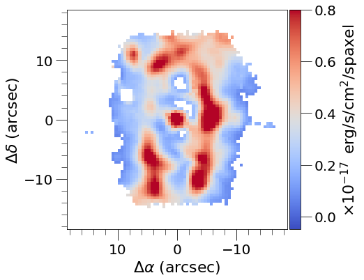
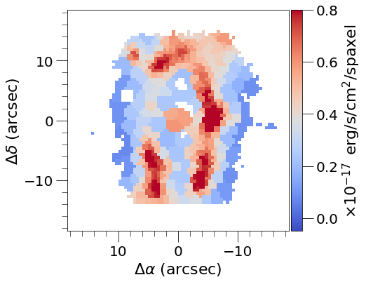
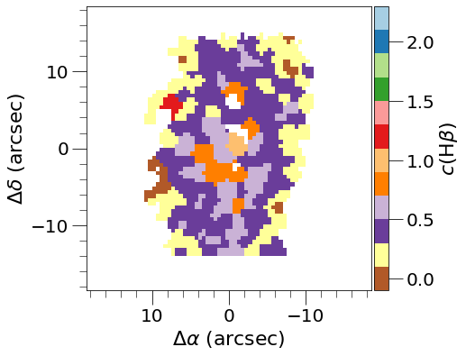
To work with reliable data, we masked all spaxels with S/N in the 2D emission-line fluxes and equivalent width maps. All emission-line intensities were reddening corrected using the extinction curve by Cardelli et al. (1989). The theoretical value used for the H/H ratio is 2.87, which was obtained for the recombination case B for an electron temperature of 10 000 K at the limit of the low density (Osterbrock & Ferland, 2006). We derived the 2D reddening coefficient [(H)] maps re-binning by S/N the H image using the publicly available Voronoi binning algorithm by Cappellari & Copin (2003). The target S/N per tessellation bin was 30 based. Figure. 1 is an example of H flux and (H) tessellated maps for the galaxy 8313-12705.
2.2 Sample selection
As mentioned in Krabbe et al. (2021), we selected objects with LINER emission in their nuclear regions and SFs emission in their disks. Furthermore, this sample is restricted to objects with LINER emission with an integrated equivalent width (EWHα) lower than 3 and higher than 0.5, which suggests that the ionization source of the nuclear region is probably post-AGBs. The sample selection followed the steps listed below.
-
1.
We used the log([O iii]5007/H) vs. log([N ii]6584/H) diagnostic diagram proposed by Baldwin et al. (1981), called BPT, to classify objects as H ii-like regions, composite, and AGN-like objects considering the theoretical and empirical criteria proposed by Kewley et al. (2001) and Kauffmann et al. (2003), respectively. The Seyfert and LINER objects are distinguished using the Kewley et al. (2006) criteria.
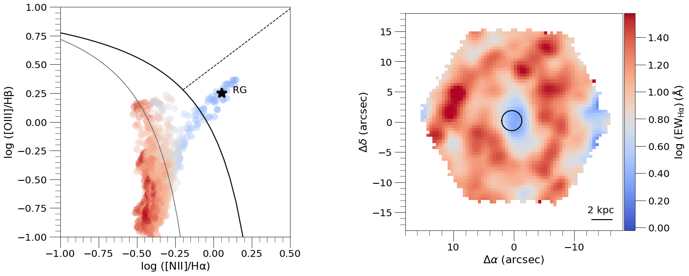
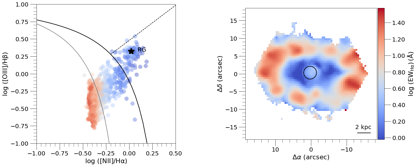
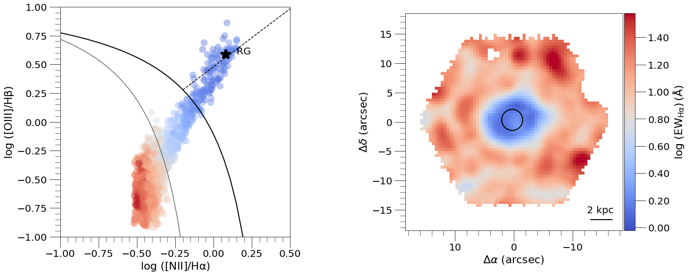
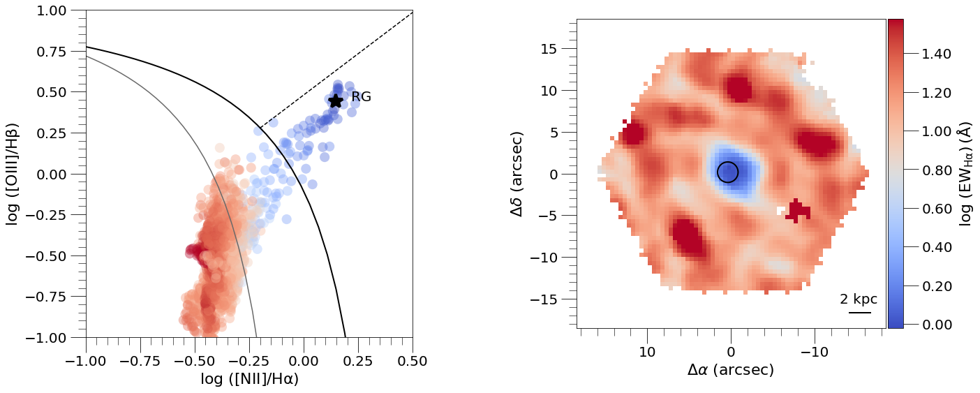
Figure 2: First column: log([O iii]5007/H) vs. log([N ii]6584/H) diagnostic diagram , from top to bottom the galaxies shown are: 7495-12704, 7990-12704, 8249-12704, and 8318-12703. The black solid curve represents the theoretical upper limit for the star-forming regions proposed by Kewley et al. (2001) (ke01); the grey solid curve is the empirical star-forming limit proposed by Kauffmann et al. (2003) (ka03); and the black dashed line represents the separation between Seyferts and LINERs (Cid Fernandes et al., 2010). The region between the Ke01 and Ka03 lines is a denominated composite region. Point colours are the same as in the second column and depend on the EWHα. Second column: spatial distribution accordingly to the . The black stars represent the integrated estimations for the nuclear regions defined by the black circles. .
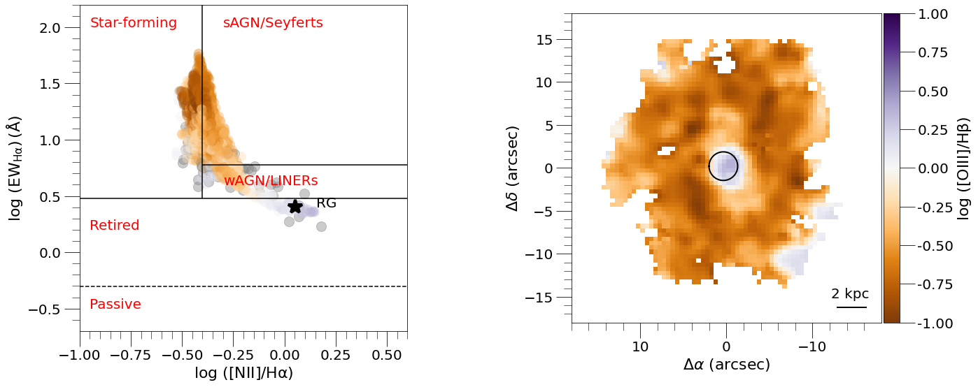
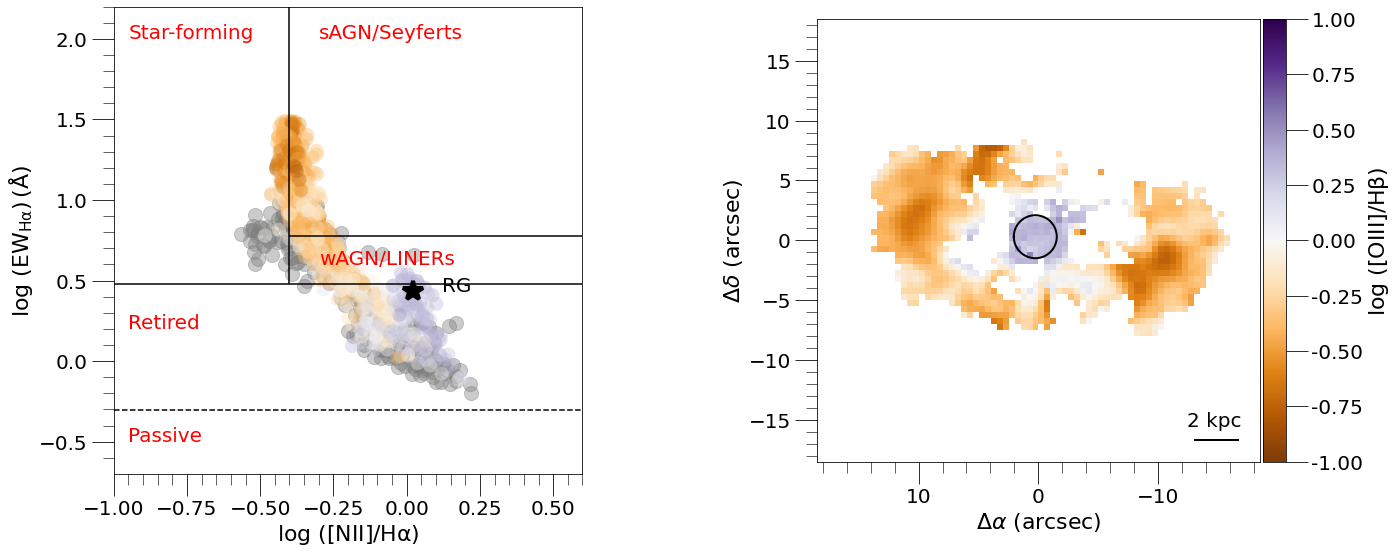
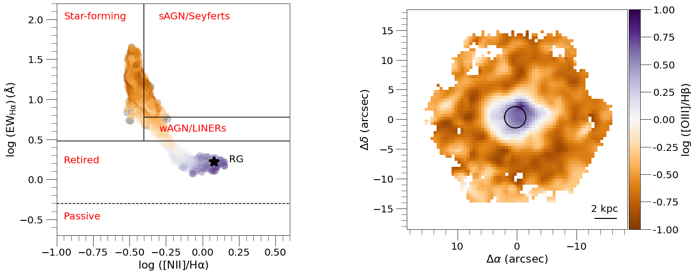
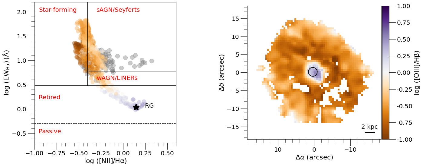
Figure 3: First column: examples of WHAN diagrams; from top to bottom the galaxies are: 7495-12704, 7990-12704, 8249-12704, and 8318-12703. Point colours are the same as in the second column and depend on the /H) ratio. Second column: spatial distribution according to the /H) ratio. The black stars represent the integrated estimations for the nuclear regions defined by the black circles. .
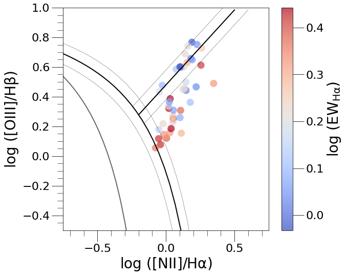
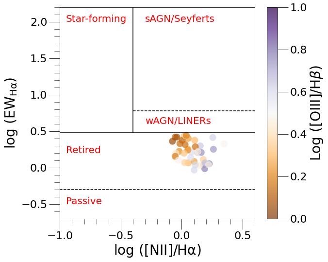
Figure 4: BPT and WHAN diagrams as shown in Fig. 2 and Fig. 3 but considering the nuclear-integrated flux for each galaxy in our sample. 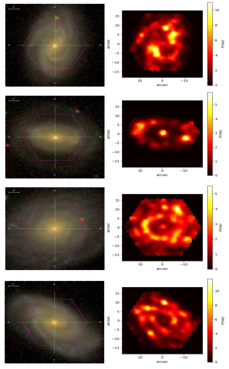
Figure 5: Left panels: SDSS image combining the gri bands of galaxies 7495-12704, 7990-12704, 8249-12704, and 8318-12703 (from top to bottom) with the MaNGA field of view indicated by the purple hexagon. Right panels: H flux spatial distribution (in units of 10-17 erg/cm2/spaxel) -
2.
We used the vs. log([N ii]6584/H) diagnostic diagram, known as WHAN (Cid Fernandes et al. 2011), to verify if the nuclear regions initially classified as LINER using the BPT diagram occupy the same area as in the WHAN diagram. The WHAN diagram is useful to differentiate the nature of the ionization sources of LINERs, i.e., between evolved low-mass stars (like post-AGB stars) and low ionization AGNs. Using the , this diagram classifies objects into five classes of galaxies, namely:
-
(a)
Pure star forming galaxies: and Å.
-
(b)
Strong AGNs: and Å.
-
(c)
Weak AGNs: and between 3 and 6 Å.
-
(d)
Retired Galaxies (RGs; i.e., fake AGNs): Å.
-
(e)
Passive galaxies (actually, line-less galaxies): and Å.
From the BPT and WHAN diagrams together with their spatial distributions we selected all objects whose nuclei are in the LINER zone in the first diagram and the RG zone in the second. We also required that the disk spaxels be in the SF zone of both diagrams. The BPT and WHAN diagrams are in Fig. 2 and Fig. 3, respectively, together with their spatial distributions, for the galaxies 7495-12704, 7990-12704, 8249-12704, and 8318-12703 belonging to our final sample. At this step, we selected all objects with the same spatial distribution pattern, following the procedures below.
-
(a)
-
3.
A circular aperture with a radius of 1 kpc was defined for each galaxy selected earlier. The integrated flux for each emission line considered was obtained for all nuclei in our sample by summing together all fluxes in this region. The BPT and WHAN diagrams were repeated for the nuclear regions of the galaxies and are shown in Fig. 4. We also include in this figure, as a black star, the nuclear integrated line ratios in the corresponding diagrams for each object, as shown in Fig. 2 and Fig. 3. Finally, we selected all objects whose integrated nuclear emission is located in the LINER and RG zones in the BPT and WHAN diagrams, respectively. For the BPT diagram (Fig. 4), deviations of 0.1 dex were considered for the lines that represent the separation between Seyferts/LINERs and AGNs-like/SFs. These variations were assumed because according to Kewley et al. (2001), the lines separating the different regions have errors in the order of 0.1 dex, which are from the modelling due to the assumptions made in the chemical abundances, chemical depletion factors, slope of the initial mass function, and stellar atmosphere models (Kewley et al., 2001).
The final sample consists of 43 galaxies with a LINER type nucleus. The stellar mass of the hosting galaxies is in the range of and the redshift is in the range of . For each galaxy of our sample, Table 1 lists the identification number of the plate, coordinates, redshift, distance, and integrated stellar mass. All information was taken from the manga.Pipe3D444https://data.sdss.org/datamodel/files/MANGA_PIPE3D and manga.drpall555https://data.sdss.org/datamodel/files/MANGA_SPECTRO_REDUX(see Sánchez et al. 2016). Fig. 5 is the RGB SDSS image (combining the gri bands) of the galaxies 7495-12704, 7990-12704, 8249-12704, and 8318-12703 together with the MaNGA field of view and the 2D maps of the spatial distribution of H flux. In Table 2, the reddening corrected emission line intensities, the reddening coefficient [(H)], and the equivalent widths of for each LINER nucleus are listed.
| Plate-IFU | RA | DEC | redshift | distance | |
|---|---|---|---|---|---|
| (deg) | (deg) | (Mpc) | |||
| 7495-12704 | 205.4384 | 27.0048 | 0.0292 | 125.29 | 10.72 |
| 7977-3704 | 332.7987 | 11.8007 | 0.0272 | 116.48 | 10.36 |
| 7977-12703 | 333.2018 | 13.3341 | 0.0744 | 330.60 | 11.00 |
| 7990-6103 | 261.2849 | 58.7647 | 0.0296 | 125.33 | 10.32 |
| 7990-12704 | 262.4861 | 58.3974 | 0.0271 | 116.46 | 10.51 |
| 8083-12704 | 50.6968 | 0.1494 | 0.0231 | 98.90 | 10.44 |
| 8131-9102 | 112.2214 | 41.3078 | 0.0586 | 256.17 | 9.97 |
| 8140-12703 | 117.8985 | 42.8801 | 0.0323 | 138.58 | 10.83 |
| 8243-9102 | 130.8217 | 52.7579 | 0.0591 | 260.66 | 11.10 |
| 8243-12701 | 128.6877 | 52.7157 | 0.0452 | 196.78 | 11.16 |
| 8247-3701 | 136.6714 | 41.3651 | 0.0252 | 107.68 | 10.35 |
| 8249-12704 | 137.3775 | 45.9524 | 0.0271 | 116.46 | 10.67 |
| 8252-12702 | 145.5309 | 48.1549 | 0.0339 | 143.10 | 10.88 |
| 8254-3704 | 164.0822 | 43.7549 | 0.0362 | 156.36 | 10.76 |
| 8257-1902 | 166.2978 | 46.1029 | 0.0371 | 160.81 | 10.64 |
| 8258-12704 | 167.7765 | 43.6330 | 0.0253 | 107.68 | 10.79 |
| 8259-9102 | 178.5399 | 44.3661 | 0.0620 | 274.51 | 10.99 |
| 8313-9102 | 239.9880 | 41.4778 | 0.0335 | 143.05 | 10.72 |
| 8313-12705 | 242.6825 | 41.1486 | 0.0319 | 134.22 | 10.91 |
| 8318-12703 | 196.2324 | 47.5036 | 0.0396 | 169.85 | 10.99 |
| 8320-9102 | 206.8303 | 21.8338 | 0.0527 | 228.69 | 11.02 |
| 8332-12705 | 209.2520 | 43.3620 | 0.0333 | 143.03 | 10.93 |
| 8330-9102 | 205.0114 | 40.4209 | 0.0245 | 103.31 | 10.45 |
| 8332-6103 | 207.6574 | 43.7641 | 0.0489 | 210.51 | 10.58 |
| 8440-12704 | 136.1423 | 41.3978 | 0.0274 | 116.49 | 10.54 |
| 8481-1902 | 237.6539 | 53.3906 | 0.0654 | 288.53 | 10.77 |
| 8482-12703 | 245.5031 | 49.5208 | 0.0500 | 215.07 | 10.96 |
| 8549-3703 | 241.4164 | 46.8466 | 0.0575 | 251.55 | 10.67 |
| 8550-6103 | 247.6387 | 39.8307 | 0.0249 | 103.36 | 10.41 |
| 8550-12704 | 247.0584 | 40.3138 | 0.0334 | 143.04 | 10.72 |
| 8550-12705 | 249.1357 | 39.0279 | 0.0303 | 129.72 | 11.04 |
| 8552-9101 | 226.9119 | 44.5563 | 0.0664 | 293.17 | 10.86 |
| 8601-12705 | 250.1231 | 39.2351 | 0.0300 | 129.68 | 10.47 |
| 8588-9101 | 250.1562 | 39.2216 | 0.0355 | 151.95 | 10.63 |
| 8138-3702 | 116.0979 | 44.5277 | 0.0500 | 215.07 | 10.72 |
| 8138-9101 | 117.3026 | 45.5103 | 0.0535 | 233.21 | 10.84 |
| 8482-3704 | 245.4124 | 49.4488 | 0.0328 | 138.65 | 10.86 |
| 8482-9101 | 241.7996 | 48.5726 | 0.0437 | 187.85 | 10.84 |
| 8554-1902 | 183.1133 | 35.8835 | 0.0231 | 98.90 | 10.02 |
| 8603-12703 | 247.2827 | 40.6650 | 0.0303 | 129.71 | 10.49 |
| 8604-12703 | 247.7642 | 39.8385 | 0.0309 | 129.79 | 10.79 |
| 8604-6102 | 246.0735 | 39.2110 | 0.0303 | 129.72 | 10.68 |
| 8606-3702 | 253.7939 | 36.9063 | 0.0239 | 98.97 | 10.30 |
| Plate-IFU | [O ii] 3727 | H | [O iii] 5007 | H | [N ii] 6584 | (H) | |
|---|---|---|---|---|---|---|---|
| 7495-12704 | 1.77 0.03 | 1.00 0.01 | 1.79 0.01 | 2.87 0.01 | 3.25 0.01 | 2.52 0.05 | 0.36 |
| 7977-3704 | 5.06 0.09 | 1.00 0.02 | 1.65 0.02 | 2.87 0.01 | 2.73 0.02 | 1.68 0.04 | 0.40 |
| 7977-12703 | 3.93 0.24 | 1.00 0.06 | 1.31 0.06 | 2.87 0.03 | 2.54 0.03 | 2.62 0.08 | 0.31 |
| 7990-6103 | 11.40 0.30 | 1.00 0.04 | 2.71 0.05 | 2.87 0.02 | 2.57 0.01 | 1.58 0.07 | 0.24 |
| 7990-12704 | 4.35 0.04 | 1.00 0.01 | 2.10 0.01 | 2.87 0.01 | 3.01 0.01 | 2.72 0.06 | 0.28 |
| 8083-12704 | 2.27 0.03 | 1.00 0.01 | 1.32 0.01 | 2.87 0.01 | 2.90 0.01 | 2.38 0.06 | 0.26 |
| 8131-9102 | 25.56 0.91 | 1.00 0.09 | 4.55 0.12 | 2.87 0.04 | 4.35 0.01 | 1.09 0.05 | 0.33 |
| 8140-12703 | 8.77 0.18 | 1.00 0.02 | 1.87 0.03 | 2.87 0.01 | 3.23 0.01 | 1.79 0.04 | 0.41 |
| 8243-9102 | 10.61 0.35 | 1.00 0.04 | 3.09 0.04 | 2.87 0.02 | 6.39 0.01 | 2.12 0.04 | 0.54 |
| 8243-12701 | 12.46 0.30 | 1.00 0.04 | 4.26 0.05 | 2.87 0.02 | 4.08 0.02 | 1.99 0.05 | 0.52 |
| 8247-3701 | 3.58 0.03 | 1.00 0.01 | 1.44 0.01 | 2.87 0.01 | 3.06 0.01 | 2.08 0.03 | 0.29 |
| 8249-12704 | 4.25 0.06 | 1.00 0.02 | 3.88 0.02 | 2.87 0.01 | 3.45 0.01 | 1.64 0.04 | 0.34 |
| 8252-12702 | 27.75 0.53 | 1.00 0.06 | 5.86 0.06 | 2.87 0.02 | 4.44 0.01 | 0.97 0.03 | 0.40 |
| 8254-3704 | 5.62 0.21 | 1.00 0.04 | 2.04 0.05 | 2.87 0.03 | 3.25 0.02 | 1.17 0.05 | 0.55 |
| 8257-1902 | 3.90 0.06 | 1.00 0.01 | 1.40 0.02 | 2.87 0.01 | 2.77 0.01 | 2.14 0.03 | 0.45 |
| 8258-12704 | 35.74 0.38 | 1.00 0.04 | 5.64 0.04 | 2.87 0.01 | 4.84 0.01 | 1.13 0.04 | 0.26 |
| 8259-9102 | 8.45 0.29 | 1.00 0.05 | 2.44 0.06 | 2.87 0.02 | 3.08 0.02 | 2.74 0.06 | 0.42 |
| 8313-9102 | 5.05 0.11 | 1.00 0.03 | 2.30 0.03 | 2.87 0.02 | 4.32 0.02 | 1.30 0.05 | 0.31 |
| 8313-12705 | 5.55 0.09 | 1.00 0.02 | 3.16 0.03 | 2.87 0.02 | 4.02 0.02 | 1.53 0.05 | 0.38 |
| 8318-12703 | 4.19 0.14 | 1.00 0.04 | 2.77 0.05 | 2.87 0.03 | 4.02 0.04 | 1.07 0.05 | 0.40 |
| 8320-9102 | 4.70 0.16 | 1.00 0.04 | 2.81 0.05 | 2.87 0.03 | 3.82 0.03 | 1.63 0.06 | 0.36 |
| 8332-12705 | 18.37 0.35 | 1.00 0.04 | 4.46 0.05 | 2.87 0.02 | 4.46 0.01 | 1.16 0.03 | 0.47 |
| 8330-9102 | 2.29 0.07 | 1.00 0.03 | 1.82 0.03 | 2.87 0.02 | 3.63 0.03 | 1.22 0.06 | 0.48 |
| 8332-6103 | 7.97 0.31 | 1.00 0.06 | 3.84 0.07 | 2.87 0.04 | 3.40 0.03 | 1.38 0.07 | 0.29 |
| 8440-12704 | 3.82 0.04 | 1.00 0.01 | 1.71 0.01 | 2.87 0.01 | 3.23 0.01 | 1.74 0.04 | 0.23 |
| 8481-1902 | 6.57 0.28 | 1.00 0.08 | 2.17 0.09 | 2.87 0.05 | 3.00 0.05 | 1.58 0.06 | 0.55 |
| 8482-12703 | 10.04 0.24 | 1.00 0.05 | 4.10 0.05 | 2.87 0.03 | 5.17 0.03 | 2.59 0.10 | 0.30 |
| 8549-3703 | 16.61 0.41 | 1.00 0.07 | 4.88 0.09 | 2.87 0.04 | 3.96 0.04 | 1.67 0.06 | 0.32 |
| 8550-6103 | 4.73 0.04 | 1.00 0.01 | 1.53 0.01 | 2.87 0.01 | 3.13 0.01 | 2.77 0.05 | 0.38 |
| 8550-12704 | 10.91 0.21 | 1.00 0.05 | 2.93 0.04 | 2.87 0.02 | 4.77 0.02 | 1.10 0.05 | 0.31 |
| 8550-12705 | 9.88 0.24 | 1.00 0.04 | 3.98 0.04 | 2.87 0.02 | 3.71 0.02 | 1.10 0.04 | 0.68 |
| 8552-9101 | 6.49 0.22 | 1.00 0.05 | 1.43 0.06 | 2.87 0.03 | 3.71 0.03 | 1.94 0.06 | 0.33 |
| 8601-12705 | 3.48 0.17 | 1.00 0.03 | 1.51 0.04 | 2.87 0.02 | 2.54 0.02 | 1.43 0.06 | 0.55 |
| 8588-9101 | 3.89 0.11 | 1.00 0.02 | 1.20 0.03 | 2.87 0.01 | 2.62 0.02 | 2.63 0.06 | 0.49 |
| 8138-3702 | 13.32 0.26 | 1.00 0.05 | 3.98 0.05 | 2.87 0.03 | 3.86 0.01 | 1.62 0.05 | 0.74 |
| 8138-9101 | 6.30 0.31 | 1.00 0.07 | 2.32 0.08 | 2.87 0.04 | 3.04 0.04 | 1.17 0.05 | 0.32 |
| 8482-3704 | 10.00 0.13 | 1.00 0.02 | 2.03 0.02 | 2.87 0.01 | 3.67 0.01 | 2.38 0.04 | 0.52 |
| 8482-9101 | 6.56 0.19 | 1.00 0.05 | 5.51 0.05 | 2.87 0.03 | 4.15 0.02 | 1.62 0.06 | 0.51 |
| 8554-1902 | 4.16 0.05 | 1.00 0.02 | 3.00 0.02 | 2.87 0.02 | 2.70 0.01 | 1.26 0.06 | 0.29 |
| 8603-12703 | 1.86 0.06 | 1.00 0.02 | 1.14 0.02 | 2.87 0.02 | 2.41 0.02 | 2.30 0.07 | 0.27 |
| 8604-12703 | 12.39 0.15 | 1.00 0.03 | 5.35 0.03 | 2.87 0.01 | 5.23 0.02 | 1.79 0.05 | 0.48 |
| 8604-6102 | 5.46 0.06 | 1.00 0.02 | 2.87 0.02 | 2.87 0.01 | 3.91 0.01 | 1.67 0.05 | 0.38 |
| 8606-3702 | 8.84 0.12 | 1.00 0.03 | 4.00 0.03 | 2.87 0.02 | 3.63 0.01 | 0.93 0.05 | 0.48 |
3 Methods
This section describes the methodology used to derive two new oxygen abundance calibrations for LINERS by using the and indexes. To calibrate the new relations, we combined observational data with photoionization models assuming post-AGB stars as ionizing sources. In Section 3.1, we present the photoionization models used to derive oxygen abundances and ionization parameter values for the integrated fluxes from the central regions of the galaxies, and in Section 3.2, we discuss an indirect method, the determination of the nuclear oxygen abundances by extrapolating the metallicity gradients obtained through Hii regions estimations, and we compare them with those derived using the new calibrations.
3.1 Photoionization models
We built photoionization model grids using the version of the Cloudy code (Ferland et al., 2017). Post-AGB stars were considered as the ionization sources since the nuclei of the objects in our sample have been classified as RGs according to the WHAN diagnostic diagram (see Fig. 4). These models are similar to the ones used by Krabbe et al. (2021). A brief description of the input parameters is presented below.
-
1.
Spectral Energy Distribution (SED): we considered SED post-AGB star atmosphere models by Rauch (2003) assuming effective temperatures () of 50, 100, and 190 kK, with logarithm of surface gravity (g) = 6.
-
2.
Metallicity: we considered the metallicity of the gas phase (/Z⊙) equal to 0.2, 0.5, 0.75, 1.0 and 2.0. Assuming the solar oxygen abundance of 12 + (O/H)⊙ = 8.69 (Allende Prieto et al., 2001; Asplund et al., 2009), the corresponding oxygen abundance range is of . All metals were linearly scaled with , with the exception of nitrogen, in which we assumed the relation of derived by Carvalho et al. (2020) from the abundance estimates of local SFs and Seyfert 2 nuclei.
-
3.
Electron Density (): we assumed three different electron density values: = 100, 500 and 3 000 , constant along the nebular radius.
-
4.
Ionization Parameter: this parameter is defined as
(1) where [] is the number of hydrogen-ionizing photons emitted by the central ionizing object per second, [cm] is the distance from the ionization source to the inner surface of the ionized gas cloud, [cm-3] is the total hydrogen density (ionized, neutral and molecular), and [cm s-1] is the speed of light. We assumed the logarithm of in the range of , with a step of 0.5 dex, which is the same range of values assumed by Krabbe et al. (2021).
Cloudy is a unidimensional code that assumes a central ionization source, which cannot represent the real situation in gaseous nebulae. In most cases, a central ionization source cannot genuinely represent the situation, for example, for giant star-forming regions, since the stars may be spread out throughout the region (e.g., Monreal-Ibero et al. 2011). Ercolano et al. (2009) and Jamet & Morisset (2008) showed that the distribution of the hot stars (e.g. O-B stars) in relation to the gas alters the ionization structure and the electron temperature (also see Jin et al. 2022). Hence, the ionization parameter partially depends on the spatial distribution of the ionizing sources with respect to the gas. In our cases, we considered the integrated spectra of the nuclei to try to minimize the stellar distribution effect on the emergent spectra. The assumption of a single star with a representative effective temperature as the main ionizing source, as assumed in our post-AGB models, is a good approximation (see, e.g., Zinchenko et al., 2019), since in the case of giant H ii regions ionized by stellar clusters (e.g. Mayya & Prabhu 1996; Bosch et al. 2001), the hottest stars dominate the gas ionization (Dors et al., 2017).
Once the photoionization models were built, diagrams of ([O iii]/[O ii]) versus =log([N ii] 6584/H) and indexes for both the observational data and photoionization model results were obtained. Then, the oxygen abundance (O/H) and the ionization parameter () of the gas phase of each LINER nucleus of the sample were determined by linear interpolation between the model results whose predict the nearest values to the measured emission line ratios. The methodology applied here is similar to the one adopted by Krabbe et al. (2021).
Note that , , and indexes were selected in this work because the former ratio is sensitive to the ionization degree of the gas phase, while the other two ratios mainly depend on its metallicity. The index was studied as the metallicity indicator for SFs by Storchi-Bergmann et al. (1994) and for Seyfert 2s by Carvalho et al. (2020). The index was first introduced by Alloin et al. (1979) as a metallicity indicator for SFs, and from there many calibrations have been proposed in the literature (e.g., Pettini & Pagel 2004; Pérez-Montero & Contini 2009; Marino et al. 2013). The ratio involves emission lines with close wavelengths, that makes it independent on the reddening correction and the uncertainties on the flux calibration in contrast to the index. Moreover, involves ions with similar ionization potentials, therefore, it is less dependent on the ionization parameter in comparison to .
3.2 Extrapolating the metallicity gradient
To verify the validity of our calibrations, we compared the oxygen abundance derived from these with measurements obtained from an independent method, which was the extrapolation of the radial oxygen abundance gradient, obtained from H ii region estimates along the galaxy disc to the central part of the host galaxies. This indirect method has been widely used in the literature (e.g., Vila-Costas & Edmunds, 1992; van Zee et al., 1998; Pilyugin et al., 2004, 2007; Zinchenko et al., 2019; Krabbe et al., 2021; do Nascimento et al., 2022) and produces an independent estimation of the nuclear metallicity.
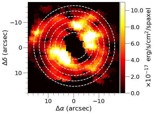
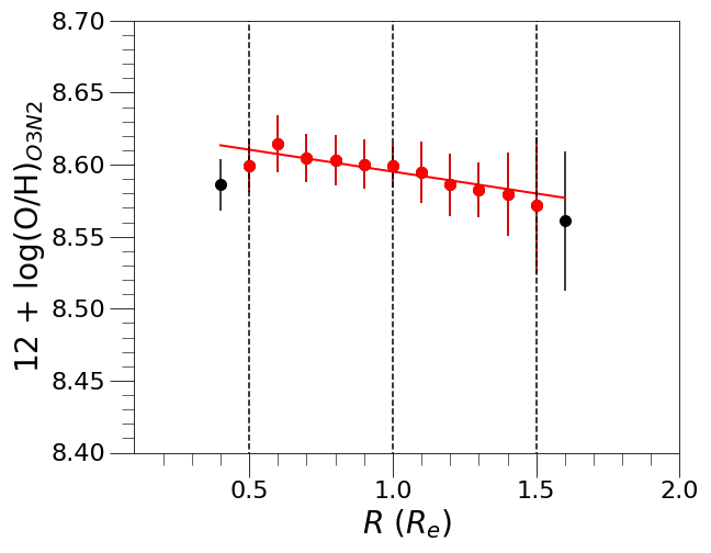
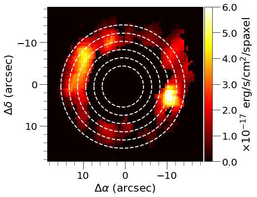
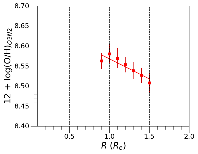
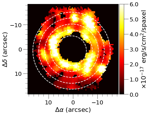
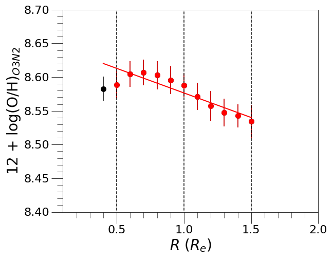
Due to the random inclination of the galaxies in the sky, the projected galactic discs are ellipticals. The radial profiles are calculated in elliptical annulus, producing some numerical artifacts. For example, the PSF beam-smearing affects the inner radii, creating a spurious flatting of the metallicity gradient at the central regions (e.g., Belfiore et al., 2017), which is worse for higher inclinations. In view of that, we calculate the metallicity gradients between 0.5 and 1.5 , where is the half-light radius of each galaxy, using a radial bin of 0.1 , and only computed the radial bin with at least 20% of the valid spaxels belonging to the corresponding annulus. Another important effect is that the annulus aperture is oversampled along the position angle of the galactic disk, while it is sub-sampled along the minor axis, yielding biased statistics inside the apertures (e.g., average and median values). To correct this, we applied a novel method introduced by Hernandez-Jimenez (in prep.) to obtain an unbiased metallicity gradient. The key step is to deproject the 2D flux maps before calculating the radial profile. To do this, we followed the recipe used by Elmegreen et al. (1992), in which the image pixels are stretched along the minor-axis by a factor of the inverse cosine of the inclination angle666Taken from the manga.drpall table.. This operation was performed by using the iraf imlintran task. We set the task to preserve the total flux of the image. In the left panels of Fig. 6, we show the deprojected 2D H maps for 7495-12704, 7990-12704, 8249-12704, and 8318-12703. In these maps, the central parts are “removed” because the ionizing sources are not young stars. The elliptical-like SF rings (see Fig. 5) observed in these galaxies are now circular due to the deprojection.
Once the 2D emission line flux maps are deprojected, we built the 2D and index maps. Afterward, we converted them into 2D metallicity abundance maps using the semi-empirical calibrations of these indexes proposed for SFs by Marino et al. (2013). These authors performed these calibrations using observations of 3 423 H ii regions from the CALIFA survey based on the -method. The and calibrations are respectively given by
| (2) |
and
| (3) |
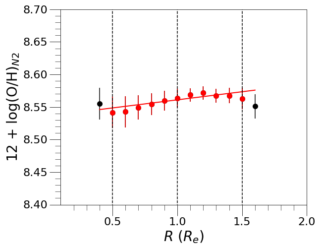
which are valid in the range for equation 2 and in the range for equation 3. Finally, we calculate the radial profile from H flux-weighted median value of the abundance map along the circular annuli. Then, the following linear fitting was obtained

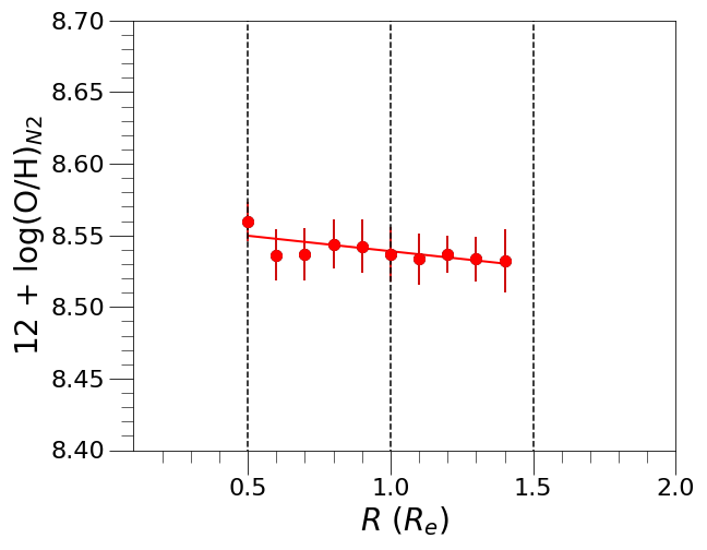
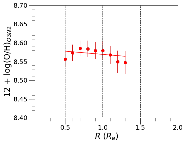
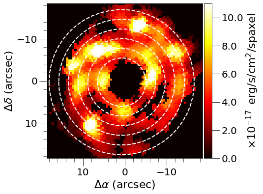
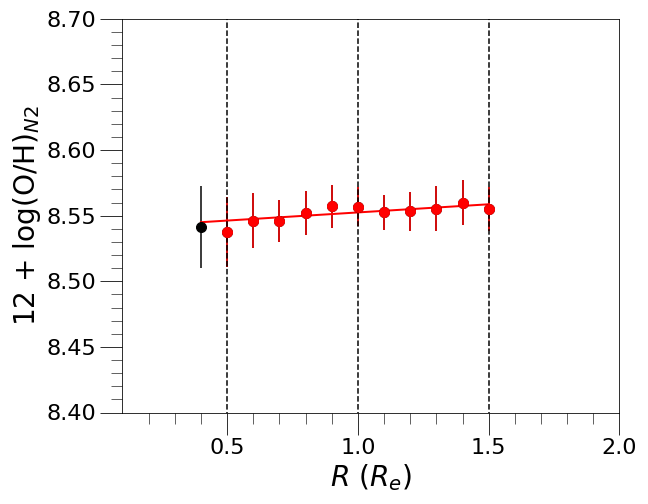
| (4) |
where is the oxygen abundance at a given galactocentric distance (in units of arcsec), is the regression slope, and is the extrapolated value of the metallicity gradient at the centre of the galaxy ( kpc). This fitting was performed for both and indexes obtaining two pairs of 12+log(O/H)0 and grad for each galaxy. We computed these metallicity gradients for galaxies with at least 5 radial bins between 0.5 and 1.5 . In this way, we were able to perform the radial fitting for 33 and 32 galaxies using the and indexes, respectively. The central and right panels of Fig. 6 present for 7495-12704, 7990-12704, 8249-12704, and 8318-12703 the metallicity gradients derived from and indexes, respectively.
4 Results
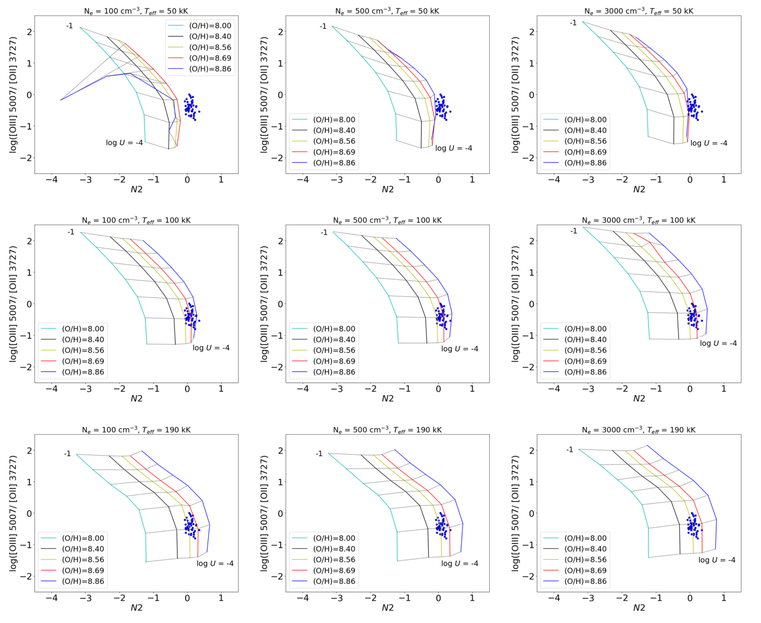
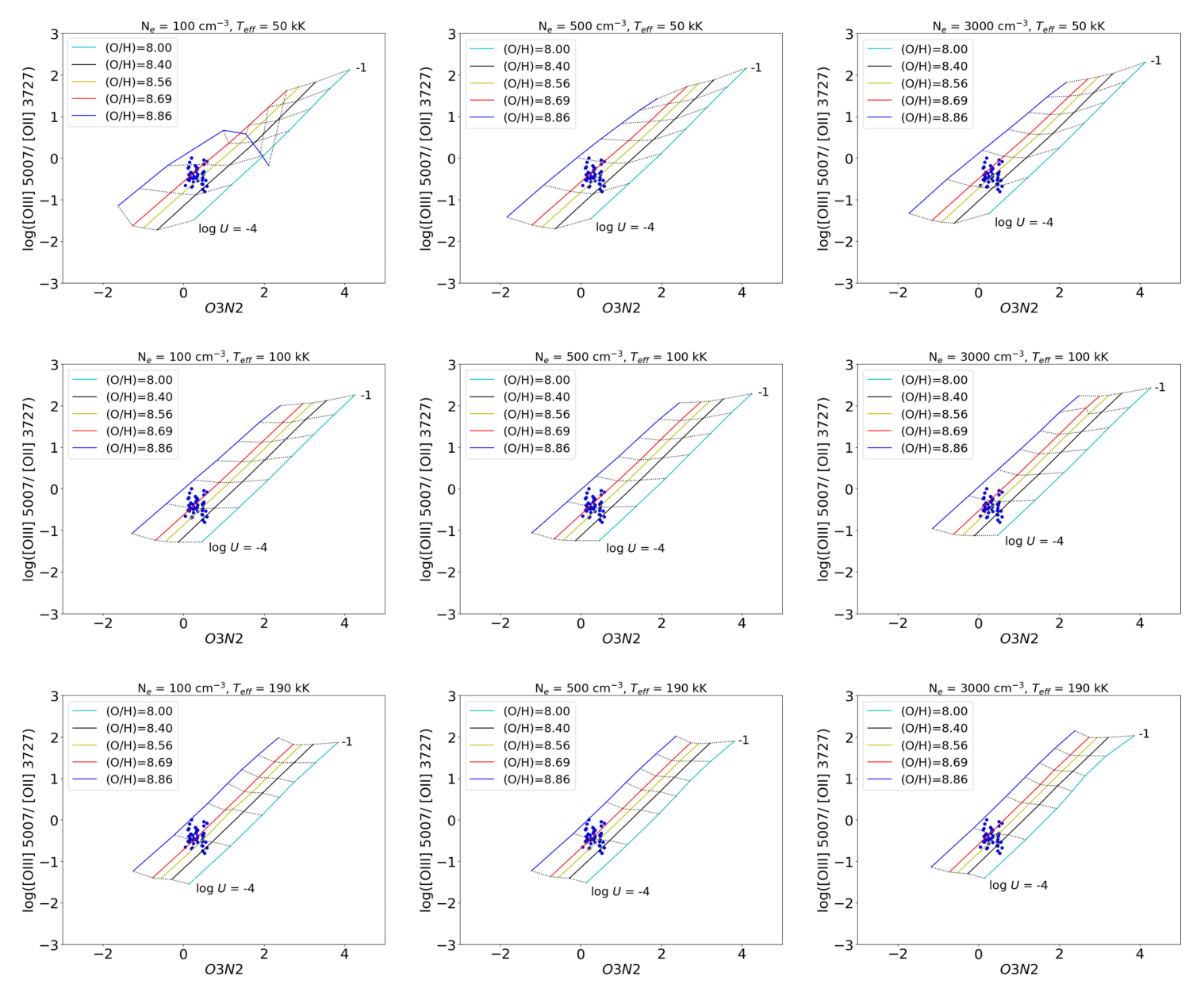
The diagnostic diagrams containing the photoionization model results and the observational data of the nuclei for the objects of our sample are shown in Figs. 7 and 8, for versus index and versus the indexes, respectively. Nine model grids with different and values are considered for the and indexes. For models with 100 and 190 kK all observational data fall within the regions occupied by the models, while models with =50 kK do not reproduce well the emission line ratios for the index. This result agrees with that found by Krabbe et al. (2021) for UGC 4805. Thus, the photoionization model results with =50 kK for the index were not taken into account in our study. The values of O/H and were derived using linear interpolations between the photoionization models following the procedure applied by Krabbe et al. (2021). In this way, we derived three pairs of points for each object: (, O/H), (, O/H) and (, ). Then, we obtained a set of point pairs for the sample and analysed the building of the calibrations.
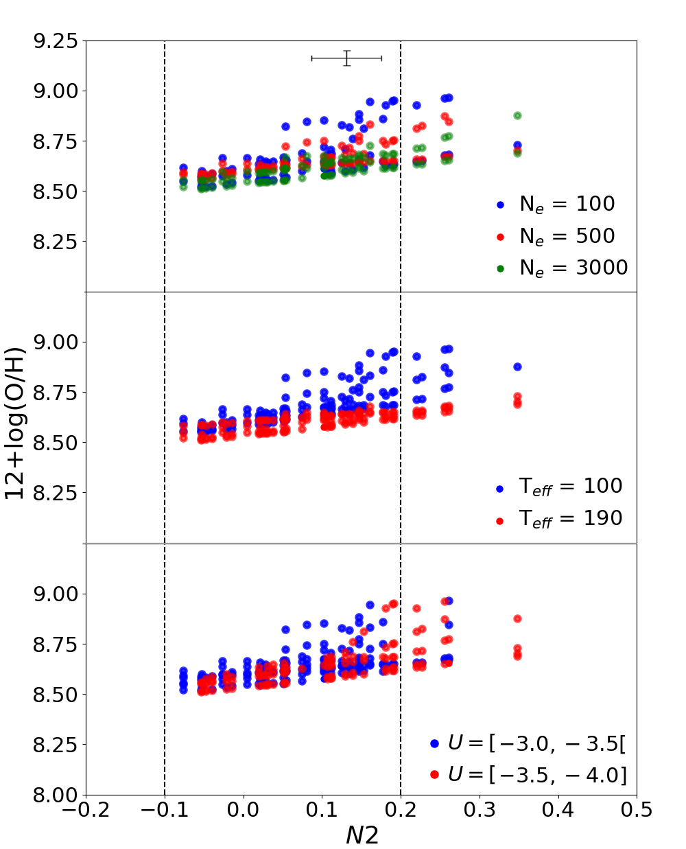
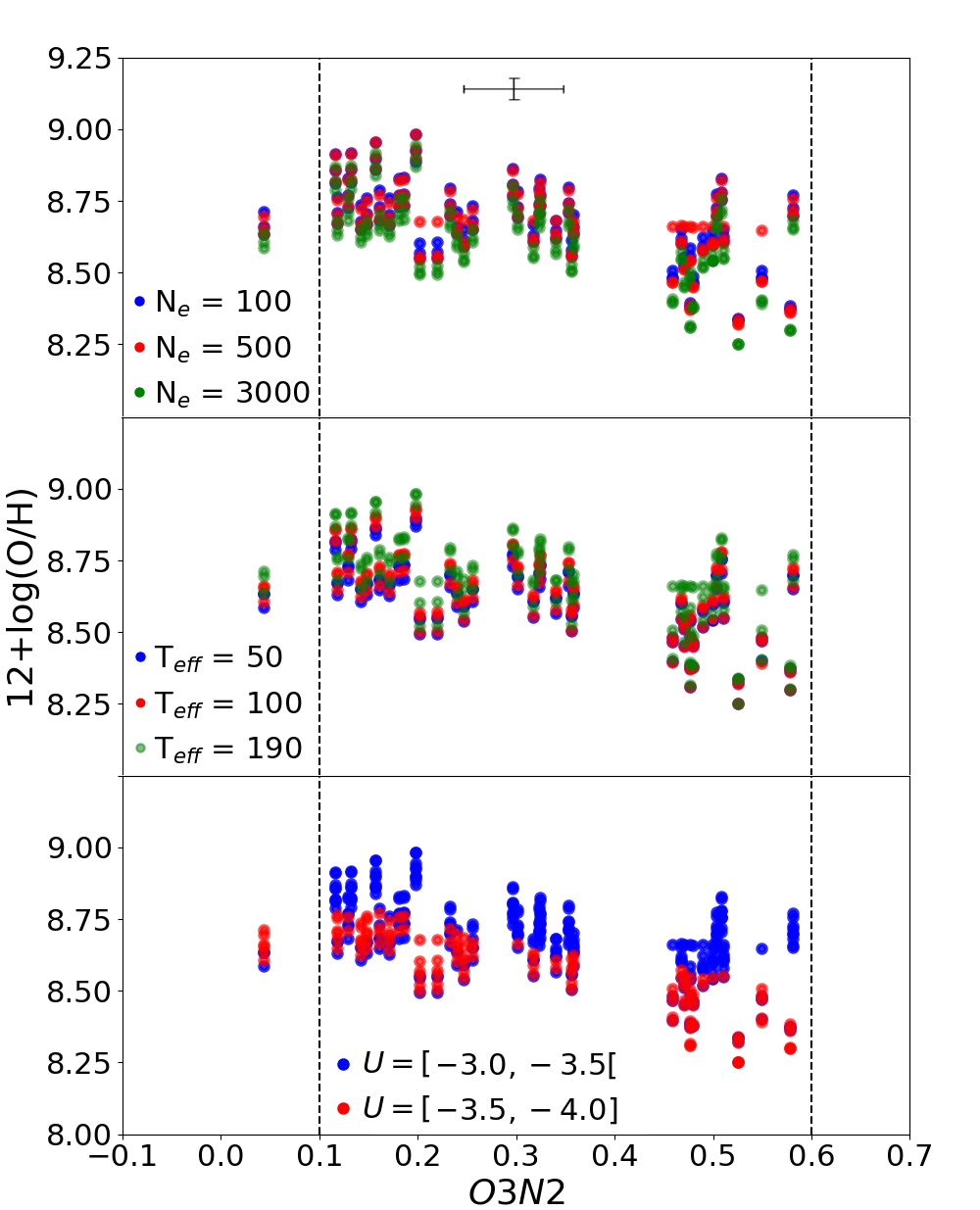
That allowed us to analyse the dependency of the oxygen abundance with , , and as a function of the and indexes, which are shown in Fig. 9. Data exhibited in this figure correspond to the interpolated model values obtained from Figs. 7 and 8 for each object, i.e., each galaxy has 6 points in each left panel of Fig. 9 and 9 points in each right panel of Fig. 9. We limited the analysis to the ranges of and , which correspond to the bulk of the observational data. For the index (left panels of Fig. 9), the higher oxygen abundance values were derived from lower values of and , without dependency on . On the other hand, for the index, the oxygen abundance is dependent on the , and , in that the higher oxygen abundance was derived from the lower values of density and higher values of effective temperature and ionization parameter. However, as seen in Fig. 9, the average error in the observational values of and produces uncertainties in the abundance estimations in the order of or even larger than those due to the variation of the nebular parameters (see also Carvalho et al. 2020).
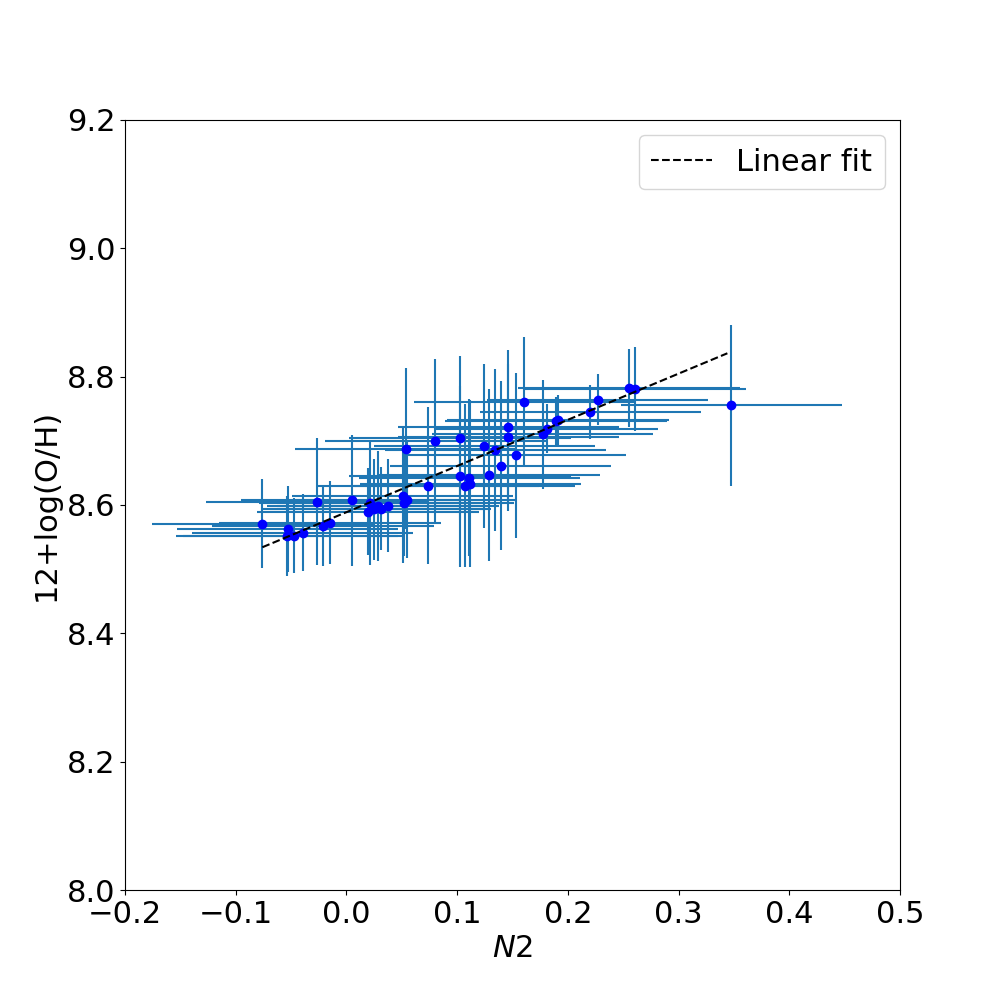
Therefore, using the orthogonal distance regression (ODR) method, which takes into account errors in both the x and y variables (Boggs & Rogers, 1990), we performed two unidimensional semi-empirical calibration considering all points, i.e., for each galaxy the assumed oxygen abundance value is the average of the interpolations for the six photoionization grid models from Fig. 7 and the nine photoionization grid models from Fig. 8. Fig. 10 presents the averaged oxygen abundance values versus the and indexes (left and right panels, respectively). The index is well correlated with the oxygen abundance with low dispersion, while the index also has a linear correlation with the oxygen abundance, but with a higher dispersion. The derived linear calibrations are given by
| (5) |
and
| (6) |

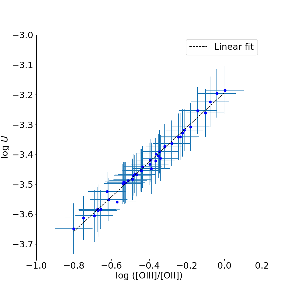
The interpolated values from Figs. 7 and 8 can also be used to derive a calibration between the observed log([O iii]/[O ii]) and the ionization parameter , which is assumed as the average, for each object, of the interpolated model values. Fig 11 contains these values, together with the obtained linear regression fit given by
| (7) |
where x=log([O iii]/[O ii]). We did not find any dependence of this relation on , and O/H, similar to the results obtained by Carvalho et al. (2020) for Narrow Line Regions of Seyfert 2 galaxies.
5 Discussions
In the chemical abundance determinations of the gas phase, the knowledge of the ionizing source is fundamental, especially when it is estimated using indirect methods. The nature of the ionizing source of LINERs is an open problem in astronomy, and three mechanisms have been proposed as responsible for the ionization: shocks (Heckman, 1980), accretion gas into a central black hole (AGN, Halpern & Steiner 1983; Ferland & Netzer 1983; Ho et al. 1993), and hot stars (post-AGB stars, Terlevich & Melnick 1985; Shields 1992; Taniguchi et al. 2000). In our specific case, the sample is composed by objects with a LINER nucleus, and according to the WHAN diagram are classified as retired galaxies. We argued that the LINER ionization sources of these galaxies are probably post-AGB stars spread along the gas (see also Krabbe et al. 2021). Therefore, based on this assumption, we proposed two semi-empirical calibrations between the and line ratios and the metallicity, as well as a calibration between [O iii]/[O ii] ratio and the ionization parameter derived from photoionization models assuming the ionizing sources are post-AGBs.
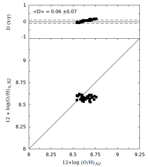
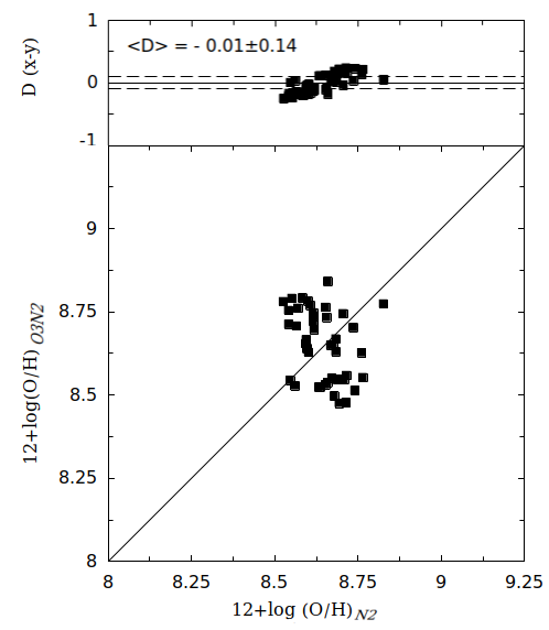
In Table 3, we list for all sampled galaxies the oxygen abundance values obtained using the calibrations proposed in this work (see Sec. 4) and those derived by extrapolating the radial gradients (see Sec. 3.2), as well as the ionization parameter values obtained by using Eq. 7. Fig. 12 shows versus through the index (left panel) and those through the index (right panel). Both and relations produced higher oxygen abundance values than those derived by the oxygen abundance gradient extrapolation method. Taking into account the observational uncertainties ( dex, Kennicutt et al. 2003) and the accuracy of the theoretical and (semi)empirical calibrations ( dex, e.g., Kewley & Dopita 2002, Carvalho et al. 2020, Dors 2021), we can claim that the present estimated abundances through the different methods agree with each other. Therefore, these estimations support the validity of the semi-empirical calibration for LINER objects obtained in this work. Using these calibrations, we found that LINERs exhibit an oxygen abundance range , with a mean value of . Fig. 13 contains a comparison between the abundance values obtained using our two calibrations. and oxygen abundance estimations are in agreement. However, this relation has a high dispersion, and the difference between both estimations (upper panel) exhibits a systematic linear behaviour. Therefore, considering these results and that the calibration presents a higher dispersion than the (see Fig. 10), even if we are able to use both calibrations to estimate the central oxygen abundance of LINER galaxies, we recommend using the calibration.

| Plate-IFU | 12+log(O/H) | 12+log(O/H)0 | |||||
|---|---|---|---|---|---|---|---|
| 7495-12704 | 8.62 0.02 | 8.74 0.05 | 3.19 0.01 | 8.54 0.02 | 8.63 0.02 | ||
| 7977-3704 | 8.57 0.01 | 8.71 0.06 | 3.47 0.02 | 8.61 0.02 | 8.56 0.03 | ||
| 7977-12703 | 8.54 0.00 | 8.75 0.05 | 3.46 0.01 | 8.60 0.01 | 8.58 0.02 | ||
| 7990-6103 | 8.55 0.01 | 8.54 0.08 | 3.55 0.02 | 8.61 0.02 | 8.60 0.03 | ||
| 7990-12704 | 8.59 0.01 | 8.67 0.06 | 3.37 0.01 | 8.61 0.03 | 8.67 0.05 | ||
| 8083-12704 | 8.58 0.01 | 8.79 0.04 | 3.32 0.01 | 8.56 0.02 | 8.72 0.03 | ||
| 8131-9102 | 8.71 0.06 | 8.55 0.08 | 3.62 0.02 | 8.58 0.04 | 8.56 0.09 | ||
| 8140-12703 | 8.62 0.02 | 8.72 0.05 | 3.57 0.02 | 8.56 0.02 | 8.62 0.02 | ||
| 8243-9102 | 8.83 0.12 | 8.77 0.05 | 3.50 0.02 | - | - | ||
| 8243-12701 | 8.69 0.04 | 8.55 0.08 | 3.46 0.01 | 8.57 0.02 | 8.62 0.02 | ||
| 8247-3701 | 8.60 0.02 | 8.78 0.04 | 3.42 0.01 | 8.61 0.02 | 8.61 0.05 | ||
| 8249-12704 | 8.64 0.03 | 8.52 0.09 | 3.21 0.01 | 8.56 0.02 | 8.59 0.03 | ||
| 8252-12702 | 8.71 0.02 | 8.48 0.09 | 3.58 0.01 | - | - | ||
| 8254-3704 | 8.62 0.01 | 8.70 0.06 | 3.44 0.01 | 8.54 0.02 | 8.59 0.02 | ||
| 8257-1902 | 8.57 0.01 | 8.76 0.05 | 3.44 0.02 | 8.62 0.03 | 8.60 0.04 | ||
| 8258-12704 | 8.74 0.05 | 8.51 0.09 | 3.65 0.01 | 8.60 0.04 | 8.54 0.06 | ||
| 8259-9102 | 8.60 0.04 | 8.63 0.07 | 3.50 0.01 | 8.54 0.02 | 8.61 0.02 | ||
| 8313-9102 | 8.71 0.04 | 8.74 0.05 | 3.38 0.01 | 8.61 0.01 | 8.64 0.03 | ||
| 8313-12705 | 8.68 0.04 | 8.63 0.07 | 3.33 0.01 | 8.61 0.02 | 8.58 0.05 | ||
| 8318-12703 | 8.68 0.06 | 8.67 0.06 | 3.29 0.02 | 8.54 0.02 | 8.65 0.02 | ||
| 8320-9102 | 8.67 0.03 | 8.65 0.07 | 3.32 0.01 | 8.58 0.02 | 8.62 0.03 | ||
| 8332-12705 | 8.72 0.02 | 8.56 0.08 | 3.54 0.01 | 8.58 0.02 | 8.62 0.03 | ||
| 8330-9102 | 8.65 0.02 | 8.76 0.05 | 3.25 0.01 | - | - | ||
| 8332-6103 | 8.63 0.01 | 8.52 0.09 | 3.37 0.02 | 8.57 0.02 | 8.57 0.04 | ||
| 8440-12704 | 8.62 0.08 | 8.75 0.05 | 3.39 0.01 | 8.59 0.01 | 8.49 0.06 | ||
| 8481-1902 | 8.59 0.04 | 8.65 0.06 | 3.46 0.02 | - | - | ||
| 8482-12703 | 8.76 0.02 | 8.63 0.07 | 3.41 0.02 | 8.59 0.02 | 8.67 0.03 | ||
| 8549-3703 | 8.68 0.07 | 8.50 0.09 | 3.49 0.02 | 8.60 0.01 | 8.57 0.02 | ||
| 8550-6103 | 8.61 0.03 | 8.77 0.05 | 3.47 0.01 | 8.56 0.01 | 8.63 0.02 | ||
| 8550-12704 | 8.74 0.03 | 8.70 0.06 | 3.52 0.02 | 8.56 0.02 | 8.66 0.04 | ||
| 8550-12705 | 8.66 0.00 | 8.54 0.08 | 3.41 0.01 | 8.57 0.03 | 8.60 0.05 | ||
| 8552-9101 | 8.66 0.01 | 8.84 0.03 | 3.56 0.02 | 8.59 0.02 | 8.59 0.02 | ||
| 8601-12705 | 8.54 0.04 | 8.71 0.06 | 3.40 0.01 | 8.55 0.02 | 8.59 0.03 | ||
| 8588-9101 | 8.55 0.01 | 8.79 0.04 | 3.48 0.01 | 8.60 0.01 | 8.59 0.02 | ||
| 8138-3702 | 8.67 0.03 | 8.55 0.08 | 3.49 0.02 | - | - | ||
| 8138-9101 | 8.60 0.01 | 8.64 0.07 | 3.44 0.01 | 8.58 0.02 | 8.64 0.02 | ||
| 8482-3704 | 8.66 0.00 | 8.73 0.05 | 3.58 0.01 | 8.58 0.02 | 8.62 0.03 | ||
| 8482-9101 | 8.69 0.08 | 8.48 0.09 | 3.23 0.01 | 8.53 0.06 | - | ||
| 8554-1902 | 8.56 0.04 | 8.53 0.09 | 3.27 0.01 | - | - | ||
| 8603-12703 | 8.53 0.03 | 8.78 0.04 | 3.31 0.01 | - | - | ||
| 8604-12703 | 8.76 0.04 | 8.55 0.08 | 3.400.01 | - | - | ||
| 8604-6102 | 8.68 0.03 | 8.65 0.07 | 3.350.02 | - | - | ||
| 8606-3702 | 8.65 0.03 | 8.53 0.08 | 3.390.01 | - | - | ||
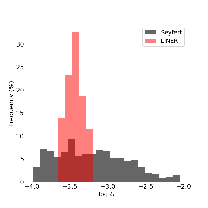
For the ionization parameter, it is well known that LINERs have a lower ionization parameter than Seyferts (see Ferland & Netzer 1983; Kewley et al. 2006). Fig. 14 compare the estimated values of the logarithm of the ionization parameter () of our sample of LINERs with those derived for a sample of Seyfert 2 galaxies studied by Carvalho et al. (2020). The values of are in the range from to and from to , for the Seyfert 2 and LINERs, respectively. The mean value of is about () and (), for the Seyfert 2 and LINER galaxies, respectively. This difference represents a factor of almost 2 on a linear scale. Hence, although some Seyferts 2 have lower ionization parameters, they extend to much higher values than the ones estimated for the LINERs. This large variation in was also reported by Stasińska (1984) for Seyfert nuclei. This author presented a series of diagrams in which different line intensity ratios are plotted for a sample of Seyfert 2 galaxies and, found that objects with low density clouds ( ) present that varies from to .
6 Conclusion
Using optical data of 43 LINER galaxies obtained from the MaNGA survey, we proposed, for the first time, two semi-empirical calibrations based on photoionization models to estimate the oxygen abundance of this class of objects, as a function of the and emission-line intensity ratios. Due to the nuclei of the objects in our sample classified as RGs according to the WHAN diagnostic diagram, we argue that these LINERs are probably ionized by post-AGB stars. Therefore, to derive the calibrations, we built photoionization models using the cloudy code considering post-AGB stars with three different effective temperatures (50, 100, 190 kK) as the ionizing sources. Using the calibrations proposed in this work, we found that LINERs exhibit an oxygen abundance range , with a mean value of . We compared the results produced by both calibrations and found they are in agreement. Comparing the results produced by the calibrations, taking into account the observational and theoretical errors, we found good agreement. Considering this result and that the calibration presents a much smaller dispersion than the calibration, we recommend the use of the index to estimate the oxygen abundances of LINERs. We compared the metallicities values produced by the proposed calibrations, with those derived by extrapolating the disk oxygen abundance gradients to the centre of the galaxies, finding that they are in good agreement. We also derived a calibration between the logarithm of the ionization parameter and the emission-line ratio.
Acknowledgements
CBO is grateful to the Fundação de Amparo à Pesquisa do Estado de São Paulo (FAPESP) for the support under grant 2019/11934-0 and to the Coordenação de Aperfeiçoamento de Pessoal de Nível Superior (CAPES). ACK thanks FAPESP for the support grant 2020/16416-5 and the Conselho Nacional de Desenvolvimento Científico e Tecnológico (CNPq). JAHJ acknowledges support from FAPESP, process number 2021/08920-8. OLD is grateful to FAPESP and CNPq. IAZ acknowledges support by the National Academy of Sciences of Ukraine under the Research Laboratory Grant for young scientists No. 0120U100148. AFM gratefully acknowledges support from CAPES.
7 Data Availability
The data underlying this article will be shared on reasonable request to the corresponding author.
References
- Aguado et al. (2019) Aguado D. S., et al., 2019, ApJS, 240, 23
- Allende Prieto et al. (2001) Allende Prieto C., Lambert D. L., Asplund M., 2001, ApJ, 556, L63
- Alloin et al. (1979) Alloin D., Collin-Souffrin S., Joly M., Vigroux L., 1979, A&A, 78, 200
- Alloin et al. (1992) Alloin D., Bica E., Bonatto C., Prugniel P., 1992, A&A, 266, 117
- Asplund et al. (2009) Asplund M., Grevesse N., Sauval A. J., Scott P., 2009, ARA&A, 47, 481
- Astropy Collaboration et al. (2013) Astropy Collaboration et al., 2013, A&A, 558, A33
- Astropy Collaboration et al. (2018) Astropy Collaboration et al., 2018, AJ, 156, 123
- Baldwin et al. (1981) Baldwin J. A., Phillips M. M., Terlevich R., 1981, PASP, 93, 5
- Belfiore et al. (2017) Belfiore F., et al., 2017, MNRAS, 469, 151
- Belfiore et al. (2019) Belfiore F., et al., 2019, AJ, 158, 160
- Blanton et al. (2017) Blanton M. R., et al., 2017, AJ, 154, 28
- Boggs & Rogers (1990) Boggs P. T., Rogers J. E., 1990, in Contemporary Mathematics. p. 186
- Bosch et al. (2001) Bosch G., Selman F., Melnick J., Terlevich R., 2001, A&A, 380, 137
- Bremer et al. (2013) Bremer M., Scharwächter J., Eckart A., Valencia-S. M., Zuther J., Combes F., Garcia-Burillo S., Fischer S., 2013, A&A, 558, A34
- Bundy et al. (2015) Bundy K., et al., 2015, ApJ, 798, 7
- Cappellari (2017) Cappellari M., 2017, MNRAS, 466, 798
- Cappellari & Copin (2003) Cappellari M., Copin Y., 2003, MNRAS, 342, 345
- Cardelli et al. (1989) Cardelli J. A., Clayton G. C., Mathis J. S., 1989, ApJ, 345, 245
- Carvalho et al. (2020) Carvalho S. P., et al., 2020, MNRAS, 492, 5675
- Castro et al. (2017) Castro C. S., Dors O. L., Cardaci M. V., Hägele G. F., 2017, MNRAS, 467, 1507
- Cid Fernandes et al. (2010) Cid Fernandes R., Stasińska G., Schlickmann M. S., Mateus A., Vale Asari N., Schoenell W., Sodré L., 2010, MNRAS, 403, 1036
- Cid Fernandes et al. (2011) Cid Fernandes R., Stasińska G., Mateus A., Vale Asari N., 2011, MNRAS, 413, 1687
- Díaz et al. (2007) Díaz Á. I., Terlevich E., Castellanos M., Hägele G. F., 2007, MNRAS, 382, 251
- Dors (2021) Dors O. L., 2021, MNRAS, 507, 466
- Dors et al. (2008) Dors O. L. J., Storchi-Bergmann T., Riffel R. A., Schimdt A. A., 2008, A&A, 482, 59
- Dors et al. (2015) Dors O. L., Cardaci M. V., Hägele G. F., Rodrigues I., Grebel E. K., Pilyugin L. S., Freitas-Lemes P., Krabbe A. C., 2015, MNRAS, 453, 4102
- Dors et al. (2017) Dors O. L., Hägele G. F., Cardaci M. V., Krabbe A. C., 2017, MNRAS, 466, 726
- Dors et al. (2020) Dors O. L., et al., 2020, MNRAS, 492, 468
- Drory et al. (2015) Drory N., et al., 2015, The Astronomical Journal, 149, 77
- Elmegreen et al. (1992) Elmegreen B. G., Elmegreen D. M., Montenegro L., 1992, ApJS, 79, 37
- Ercolano et al. (2009) Ercolano B., Bastian N., Stasińska G., 2009, Ap&SS, 324, 199
- Falcón-Barroso et al. (2011) Falcón-Barroso J., Sánchez-Blázquez P., Vazdekis A., Ricciardelli E., Cardiel N., Cenarro A. J., Gorgas J., Peletier R. F., 2011, A&A, 532, A95
- Ferland & Netzer (1983) Ferland G. J., Netzer H., 1983, ApJ, 264, 105
- Ferland et al. (2017) Ferland G. J., et al., 2017, Rev. Mex. Astron. Astrofis., 53, 385
- Hägele et al. (2006) Hägele G. F., Pérez-Montero E., Díaz Á. I., Terlevich E., Terlevich R., 2006, MNRAS, 372, 293
- Hägele et al. (2008) Hägele G. F., Díaz Á. I., Terlevich E., Terlevich R., Pérez-Montero E., Cardaci M. V., 2008, MNRAS, 383, 209
- Halpern & Steiner (1983) Halpern J. P., Steiner J. E., 1983, ApJ, 269, L37
- Harris et al. (2020) Harris C. R., et al., 2020, Nature, 585, 357
- Heckman (1980) Heckman T. M., 1980, A&A, 87, 152
- Hernandez-Jimenez (2022) Hernandez-Jimenez J. A., 2022, Astroplotlib: Python scripts to handle astronomical images, Astrophysics Source Code Library, record ascl:2204.002 (ascl:2204.002)
- Hernandez-Jimenez et al. (2013) Hernandez-Jimenez J. A., Pastoriza M. G., Rodrigues I., Krabbe A. C., Winge C., Bonatto C., 2013, MNRAS, 435, 3342
- Hernandez-Jimenez et al. (2015) Hernandez-Jimenez J. A., Pastoriza M. G., Bonatto C., Rodrigues I., Krabbe A. C., Winge C., 2015, MNRAS, 451, 2278
- Ho et al. (1993) Ho L. C., Filippenko A. V., Sargent W. L. W., 1993, ApJ, 417, 63
- Hunter (2007) Hunter J. D., 2007, Computing in Science & Engineering, 9, 90
- Izotov & Thuan (2008) Izotov Y. I., Thuan T. X., 2008, ApJ, 687, 133
- Jamet & Morisset (2008) Jamet L., Morisset C., 2008, A&A, 482, 209
- Jensen et al. (1976) Jensen E. B., Strom K. M., Strom S. E., 1976, ApJ, 209, 748
- Jin et al. (2022) Jin Y., Kewley L. J., Sutherland R., 2022, ApJ, 927, 37
- Kauffmann et al. (2003) Kauffmann G., et al., 2003, MNRAS, 346, 1055
- Kennicutt et al. (2003) Kennicutt Robert C. J., Bresolin F., Garnett D. R., 2003, ApJ, 591, 801
- Kewley & Dopita (2002) Kewley L. J., Dopita M. A., 2002, ApJS, 142, 35
- Kewley et al. (2001) Kewley L. J., Dopita M. A., Sutherland R. S., Heisler C. A., Trevena J., 2001, ApJ, 556, 121
- Kewley et al. (2006) Kewley L. J., Groves B., Kauffmann G., Heckman T., 2006, MNRAS, 372, 961
- Kewley et al. (2019) Kewley L. J., Nicholls D. C., Sutherland R. S., 2019, ARA&A, 57, 511
- Krabbe et al. (2021) Krabbe A. C., Oliveira C. B., Zinchenko I. A., Hernández-Jiménez J. A., Dors O. L., Hägele G. F., Cardaci M. V., Telles N. R., 2021, MNRAS, 505, 2087
- López-Sánchez & Esteban (2010) López-Sánchez Á. R., Esteban C., 2010, A&A, 517, A85
- Maiolino & Mannucci (2019) Maiolino R., Mannucci F., 2019, A&ARv, 27, 3
- Marino et al. (2013) Marino R. A., et al., 2013, A&A, 559, A114
- Mayya & Prabhu (1996) Mayya Y. D., Prabhu T. P., 1996, AJ, 111, 1252
- Monreal-Ibero et al. (2011) Monreal-Ibero A., Relaño M., Kehrig C., Pérez-Montero E., Vílchez J. M., Kelz A., Roth M. M., Streicher O., 2011, MNRAS, 413, 2242
- Netzer (2013) Netzer H., 2013, The Physics and Evolution of Active Galactic Nuclei. Cambridge University Press, doi:10.1017/CBO9781139109291
- Osterbrock & Ferland (2006) Osterbrock D. E., Ferland G. J., 2006, Astrophysics of gaseous nebulae and active galactic nuclei. University Science Books
- Pagel et al. (1979) Pagel B. E. J., Edmunds M. G., Blackwell D. E., Chun M. S., Smith G., 1979, MNRAS, 189, 95
- Peimbert et al. (2017) Peimbert M., Peimbert A., Delgado-Inglada G., 2017, PASP, 129, 082001
- Pérez-Montero (2017) Pérez-Montero E., 2017, PASP, 129, 043001
- Pérez-Montero & Contini (2009) Pérez-Montero E., Contini T., 2009, MNRAS, 398, 949
- Pettini & Pagel (2004) Pettini M., Pagel B. E. J., 2004, MNRAS, 348, L59
- Pilyugin (2003) Pilyugin L. S., 2003, A&A, 399, 1003
- Pilyugin et al. (2004) Pilyugin L. S., Vílchez J. M., Contini T., 2004, A&A, 425, 849
- Pilyugin et al. (2007) Pilyugin L. S., Thuan T. X., Vílchez J. M., 2007, MNRAS, 376, 353
- Rauch (2003) Rauch T., 2003, A&A, 403, 709
- Sánchez-Blázquez et al. (2006) Sánchez-Blázquez P., et al., 2006, MNRAS, 371, 703
- Sánchez et al. (2016) Sánchez S. F., et al., 2016, Rev. Mex. Astron. Astrofis., 52, 171
- Shields (1992) Shields J. C., 1992, ApJ, 399, L27
- Singh et al. (2013) Singh R., et al., 2013, A&A, 558, A43
- Smee et al. (2013) Smee S. A., et al., 2013, AJ, 146, 32
- Stasińska (1984) Stasińska G., 1984, A&A, 135, 341
- Storchi-Bergmann et al. (1994) Storchi-Bergmann T., Calzetti D., Kinney A. L., 1994, ApJ, 429, 572
- Storchi-Bergmann et al. (1998) Storchi-Bergmann T., Schmitt H. R., Calzetti D., Kinney A. L., 1998, The AJ, 115, 909
- Taniguchi et al. (2000) Taniguchi Y., Shioya Y., Murayama T., 2000, The AJ, 120, 1265
- Terlevich & Melnick (1985) Terlevich R., Melnick J., 1985, MNRAS, 213, 841
- Toribio San Cipriano et al. (2017) Toribio San Cipriano L., Domínguez-Guzmán G., Esteban C., García-Rojas J., Mesa-Delgado A., Bresolin F., Rodríguez M., Simón-Díaz S., 2017, MNRAS, 467, 3759
- Vila-Costas & Edmunds (1992) Vila-Costas M. B., Edmunds M. G., 1992, MNRAS, 259, 121
- Virtanen et al. (2020) Virtanen P., et al., 2020, Nature Methods, 17, 261
- Wake et al. (2017) Wake D. A., et al., 2017, AJ, 154, 86
- Westfall et al. (2019) Westfall K. B., et al., 2019, AJ, 158, 231
- Winkler (2014) Winkler H., 2014, arXiv e-prints, p. arXiv:1409.2966
- Yan (2018) Yan R., 2018, MNRAS, 481, 476
- Yan & Blanton (2012) Yan R., Blanton M. R., 2012, The ApJ, 747, 61
- Zinchenko et al. (2019) Zinchenko I. A., Dors O. L., Hägele G. F., Cardaci M. V., Krabbe A. C., 2019, MNRAS, 483, 1901
- do Nascimento et al. (2022) do Nascimento J. C., et al., 2022, MNRAS, 513, 807
- van Zee et al. (1998) van Zee L., Salzer J. J., Haynes M. P., O’Donoghue A. A., Balonek T. J., 1998, AJ, 116, 2805