Can locational disparity of prosumer energy optimization due to inverter rules be limited?

Abstract

To mitigate issues related to the growth of variable smart loads and distributed generation, distribution system operators (DSO) now make it binding for prosumers with inverters to operate under pre-set rules. In particular, the maximum active and reactive power set points for prosumers are based on local voltage measurements to ensure that inverter output does not cause voltage violations. However, such actions, as observed in this work, restrict the range available for local energy management, with more adverse losses on arbitrage profits for prosumers located farther away from the substation. The goal of the paper is three-fold: (a) to develop an optimal local energy optimization algorithm for activation of load flexibility and inverter-interfaced solar PV and energy storage under time-varying electricity prices; (b) to quantify the locational impact on prosumer arbitrage gains due to inverter injection rules prevalent in different energy markets; (c) to propose a computationally efficient hybrid inverter control policy which provides voltage regulation while substantially reducing locational disparity. Using numerical simulations on three identical prosumers located at different parts of a radial feeder, we show that our control policy is able to minimize locational disparity in arbitrage gains between customers at the beginning and end of the feeder to 1.4%, while PV curtailment is reduced by 91.7% compared to the base case with restrictive volt-Var and volt-watt policy.

Abbreviation
ANRC	Avoiding Negative Reinforcement Control
CVC	Cumulative Voltage Correction
DN	Distribution Network
DG	Distributed Generation
DSO	Distribution System Operator
HVAC	Heating, Ventilation, and Air Conditioning
LCG	Loss of Consumer Gain
LP	Linear Programming
PCC	Point of Common Coupling
PRC	Positive reinforcement control
P(U)	Volt-Watt
Q(U)	Volt-Var
PV	PhotoVoltaic
TCI	Total Curtailed Energy
VCI	Voltage Correction Index
VR	Voltage regulation

I Introduction

The penetration of distributed generation (DG) and flexible loads in low voltage (LV) distribution networks (DN) is growing at an astounding pace, and near future projections point towards a substantial share of total energy consumed being met. Along with DG, prosumers with flexible loads such as water heaters, HVAC [1], pool pumps [2], and energy storage can perform local energy optimization to minimize their electricity bill. Further, distribution system operators (DSOs) motivate such LV prosumers to be responsive by introducing time-varying electricity prices, net-energy metering, peak demand charge, etc. The authors in [3, 4, 5] use thermostatically controlled load and energy storage for performing energy arbitrage, while [6] uses energy storage for peak shaving and frequency control, and [7] studies power factor correction along with arbitrage. The authors in [8, 9, 10] use energy storage for increasing photovoltaic (PV) hosting capacity. The growth of DGs in a DN causes several problems for DSO such as localized voltage rise beyond permissible limits, and reverse power flow causing damage to electrical appliances [11]. In order to mitigate these issues, DSOs choose either or a combination of four paths: (a) develop new inverter connection grid rules, (b) upgrade DN with reinforcements, such as installing tap changing transformers, etc, (c) curtail renewable generation or load in case of voltage rise/dip beyond thresholds, or (d) create a market for procuring prosumer load flexibility directly or through an aggregator. Indeed, IEEE-1547-2018 standard makes it mandatory for incoming DGs to comply with voltage regulation capabilities [12, 13] to minimize system violations, as summarized in Table I. The standard promotes operation modes such as (a) constant power factor mode, (b) constant reactive power mode, (c) volt-Var, (d) P-Q mode, and (f) volt-watt mode.

TABLE I: Desired capabilities according to IEEE-1547-2018 [12, 13]

	Mandatory voltage regulation capability modes
Performance Categories	Constant power factor ($\cos\phi$)	Constant reactive power	Voltage-reactive power (volt-Var)	Active power-reactive power	Voltage-active power (volt-watt)
Category A: Minimum performance	yes	yes	yes	Not required	Not required
Category B: for smart inverters	yes	yes	yes	yes	yes

In Europe, inverter control rules are also commonly used by the DSOs [14, 15]. This involves controlling the active (P) and reactive (Q) power output of the inverter as a function of local voltage measurements (U). This is also referred to as volt-watt and volt-Var control in literature [16]. As an example, reactive power injection rules are shown in Table II for Mitnetz Strom, a DSO in Eastern Germany [17]

TABLE II: Mitnetz Strom inverter operational modes [17]

	Inverter $\leq$ 4.6 kVA	Inverter $\geq$ 4.6 kVA
Desired $\cos\phi$	0.95	0.9
Generation	1) $\cos\phi$ (P) characteristic	1) Volt-Var
	2) Fixed $\cos\phi$	2) $\cos\phi$ (P) characteristic
		3) Fixed $\cos\phi$
Storage	1) Fixed $\cos\phi$	1) Volt-Var
		2) Fixed $\cos\phi$

P(U) and Q(U) inverter control in standalone and/or in combination have been studied in [18, 19, 20, 21] for performing localized voltage regulation, ensuring DN voltage does not aggravate due to additional injection or consumption of P and Q. The authors in [22, 23, 24] use Q(U) control with active power curtailment as a last resort for mitigating overvoltages caused by PV injection. In [25], the authors propose reactive power control envelopes based on the unused solar inverter capacity for ensuring nodal voltages are within bounds. However, [22, 25] do not consider local optimization of prosumers. Authors in [26, 27] propose centralized dispatch of PV inverters for avoiding voltage issues and minimizing curtailment. However, centralized control for small-sized inverters is not practical as it requires feedback from local measurements, which is ineffective in DNs due to the incomplete spread of smart meters [28] and privacy concerns [29]. This motivates us to focus on studying distributed inverter control with optimizing flexible prosumer’s energy cost.

In recent years, many works have highlighted the disparity caused in inverter usage due to prosumer location in a radial DN. [30] proposes a PV hosting capacity mechanism in presence of inverter control policies such as volt-var and volt-watt, where they exemplify the locational impact of prosumer PV connection. Authors in [31] underscore that the DN relay settings are affected by the location of DN protection relay in a radial DN. They utilize relay settings as a basis for DG placement. In [32], an assessment is performed to quantify the locational impact on the lifetime of PV inverters. The authors conclude that the operational life of the inverter is significantly affected by the installation site along with ambient temperatures. In radial DN, the voltage levels drop as one moves farther away from the feeder head or substation [33, 34], leading to greater voltage fluctuations at farther locations. Hence, current local inverter rules will lead to different operational regimes for prosumers at different locations and affect their arbitrage opportunity. In this work, we will analyze locational impacts on load flexibility and arbitrage due to volt-Var and volt-watt modes of inverter control in detail. To this end, we design new hybrid modes for inverter control that remedy the locational disparity. It is worth noting that our study is in line with the mandate that DSOs should broadly provide a level-playing field for all prosumers consuming or injecting electrical energy, irrespective of prosumer location [35].

Contributions: The goal of the paper is to quantify the locational discrepancy for a prosumer with DG, energy storage, and flexible load due to contemporary DSO rules which enforce active and reactive power limits on inverter-interfaced generation. The prosumer considered in this paper is shown in Fig. 1.

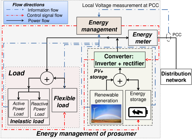
Figure 1: Prosumer energy management with voltage regulation at the point of common coupling (PCC) using local voltage measurement

The main contributions of the paper are:

• To evaluate the economic value of energy storage and load flexibility, using an LP (linear programming) based formulation for resource dispatch and further to quantify the locational disparity of prosumers that perform local energy optimization while following inverter control rules that ensure grid voltages are within the safe operational region.

• To propose a novel local hybrid inverter control policy that minimizes the locational disparity and is computationally efficient. We compare our approach against two traditional inverter policies: (a) positive reinforcement control (PRC) and (b) avoiding negative reinforcement control (ANRC), which represent an optimistic and pessimistic interpretation of volt-Var and volt-watt control policies.

Using the proposed framework, we observe the loss of consumer profit due to inverter control and note that a prosumer at the end of the feeder may have to pay more than 43% in the variable component of their electricity bill, compared to a similar prosumer located near the distribution substation. Moreover, we observe that passive inverter rules may fail if a large capacity energy storage device is connected at a node, as storage can reverse the mode of operation, i.e. from charging to discharging and vice versa, which may cause voltage violation in the opposite direction compared to the direction of correction. Crucially, we observe that a hybrid inverter control policy where active power (P) is controlled using ANRC and reactive power (Q) is controlled using PRC significantly reduces the prosumer excess cost of consumption while ensuring the correction of nodal voltage.

This paper is structured as follows. In Section II, the mathematical formulation for scheduling load flexibility and energy storage is performed using linear programming. This formulation is an extension of prior work on storage performing arbitrage proposed in [36]. Section III translates the inverter control rules into permissible ranges for an active and reactive generation. These ranges are utilized to validate the energy optimization output at a faster timescale. Section IV details the effect of the location of prosumer on DN and performance indices used, and directions in which fairness can be incorporated. Section V presents the numerical results. Section VI concludes this paper.

II Prosumer energy management

We consider a prosumer with inelastic and flexible load components, local generation, and energy storage (as shown in Fig. 1). It is connected to the DN, from where it can buy or to which it can sell energy. Based on buying and selling price fluctuations, load, and generation variations, the prosumer energy management system optimizes battery states and flexible loads at regular intervals to minimize the cost of energy. Moreover, the prosumer is obliged to follow active and reactive power injection rules as detailed in Section III. We now describe the optimization problem for the prosumer in detail.

II-A Notation and system model

The price of electricity at time instant $i$ consists of $p_{b}^{i}$ (the buying price) and $p_{s}^{i}$ (the selling price). The difference between buying and selling prices is common in DSOs [37, 38], and their ratio is denoted as $\kappa_{i}$. The end user’s inelastic consumption is denoted as $d_{i}\geq 0$, the flexible load is denoted as $y_{i}\geq 0$, and renewable generation is given as $r_{i}\geq 0$. Net uncontrolled power seen at the energy meter is denoted as $z_{i}=d_{i}-r_{i}~{}\in\mathbb{R}$.

II-A1 Timescale and notation

Prosumer energy optimization is performed at a slower timescale at every time instant $i$. The total time duration, $T$, of operation is divided into $N$ equal steps, indexed by $\{1,...,N\}$. The time duration of each step $1\leq i\leq N$ is denoted as $h$. Hence, $T=Nh$.

The time period between $i$ and $i+1$ can be divided into a faster timescale as shown in Fig. 2 and referred to using $k_{i}$. The value of $k_{i}$ resets to 0 at $i$. At this faster timescale, local voltage regulation is performed.

In this work, energy management is performed every 15 minutes, and the voltage is regulated every minute based on the voltage measurement at PCC. The grid voltage at PCC is measured every minute. Active and reactive power outputs are adjusted to satisfy the grid’s needs.

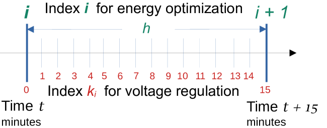
Figure 2: Pictorial representation of timescale for optimization and voltage regulation

II-A2 Flexibility model

The flexible component of the load can be controlled within a range while ensuring the cumulative energy consumed is not decreased. This is given by

$$K-\epsilon\leq h\sum_{i=1}^{N}y_{i}\leq K+\epsilon,\text{and}~{}y_{i}\in[y_{\min}^{i},y_{\max}^{i}],~{}\forall i,$$ (1)

where $K$ denotes targeted cumulative energy consumed by flexible loads (ensuring the quality of service). The flexible loads can be operated with an upper and lower envelope denoted as $y_{\max}^{i}$ and, $y_{\min}^{i}$ respectively. Note that the flexibility is derived from loads, therefore, $y_{\min}^{i}\geq 0$. (1) will ensure arbitrage benefits are due to energy management and not because of a reduction in total energy consumption. $\epsilon$ denotes a small number for ensuring total energy consumed by flexible devices is approximately equal to $K$ with a small slack. In the absence of slack, (1) is an equality constraint.

II-A3 Battery model

The battery model considers the ramping constraint, and the capacity constraint along with charging and discharging efficiencies denoted by $\eta_{\text{ch}},\eta_{\text{dis}}\in(0,1]$, respectively. The energy optimization considers the change in energy levels of the battery at time $i$ is denoted as $x_{i}$. Selection of $x_{i}$ as the decision variable ensures that the energy storage arbitrage problem is convex, provided the ratio of selling and buying price of electricity denoted as $\kappa$ satisfies $\kappa\leq 1$ [4, 36, 38]. Change in battery energy level at $i$ is defined as $x_{i}=h\delta_{i}$, where $\delta_{i}\in[\delta_{\min},\delta_{max}]$ $\forall i$ denotes ramp rate of the battery. $\delta_{i}>0$ when the battery is charging and vice versa. Note, $\delta_{i}$ is in units of power and $x_{i}$ is in units of energy. The battery charge level is denoted as

$$b_{i}=b_{i-1}+x_{i},\quad b_{i}\in[b_{\min},b_{\max}],\forall i,$$ (2)

where $b_{\min},b_{\max}$ are the minimum and maximum battery capacity. The power consumed by a battery at time $i$ is denoted as

$$f(x_{i})=\frac{[x_{i}]^{+}}{h\eta_{\text{ch}}}-\frac{\eta_{\text{dis}}[x_{i}]^{-}}{h}=\frac{1}{h\eta_{\text{ch}}}\max(0,x_{i})-\frac{\eta_{\text{dis}}\max(0,-x_{i})}{h},$$ (3)

where $x_{i}$ must lie in the range from $X_{\min}=\delta_{\min}h$ to $X_{\max}={\delta_{\max}h}$. The total power consumed between time step $i$ and $i+1$ is given as $L_{i}=z_{i}+y_{i}+f(x_{i})$, where $z_{i}$ is the uncontrolled net load, $y_{i}$ is the flexible load, and $f(x_{i})$ is the battery consumption.

The battery model is denoted as $x$C-$y$C: the battery will require $1/x$ hours to fully charge and $1/y$ hours to fully discharge.

II-B Price based energy arbitrage

The optimal arbitrage problem is defined as the minimization of the cost of consumption of energy (sum of net inflexible load, flexible load, and storage) over a time horizon considering battery constraints and load flexibility constraints.

$$\min_{x,y}h\sum_{i}^{N}[z_{i}+y_{i}+f(x_{i})]^{+}p_{\text{b}}^{i}-[z_{i}+y_{i}+f(x_{i})]^{-}p_{\text{s}}^{i},$$ (4a)

$$\text{s.t.}~{}~{}\eqref{eq:loadflexibility},$$ (4b)

$$b_{\min}-b_{0}\leq h\sum_{i}^{N}f(x_{i})\leq b_{\max}-b_{0},~{}\forall i,$$ (4c)

$$x_{i}\in[X_{\min},X_{\max}],~{}\forall i.$$ (4d)

The first constraint relates to load flexibility, the second to battery capacity, and the third to battery ramping. This formulation can be solved as a linear programming (LP) formulation, denoted as $(P_{LP})$ in Appendix -A. In the next section, we discuss the introduction of non-linear inverter size constraints that will be updated at a finer timescale based on voltage measurement.

III Inverter control and operation

III-A Inverter model

The inverter, shared by PV and battery, has a maximum $S_{\max}$ rating in Volt-Ampere (VA). Its output over each 15-minute slot, based on energy optimization in (4a), is denoted as $P_{\text{inv}}^{i}=f(x_{i})-r_{i}$, where $r_{i}$ denotes the renewable generation. Within each time-slot $i$, the inverter active power $P_{\text{inv}}^{k_{i}}$ and the storage output $P_{B}^{k_{i}}$ are modeled at a faster timescale of 1 minute (see Fig. 2), related as

$$P_{\text{inv}}^{k_{i}}=P_{B}^{k_{i}}-r_{i}+P_{\text{curt}}^{k_{i}},$$ (5)

where $P_{\text{curt}}^{k_{i}}$ denotes curtailed active power. Note $P_{\text{curt}}^{k_{i}}\in[0,r_{i}]$. The inverter power limits are given as

$$P_{\text{inv}}^{k_{i}}\in[-P_{\max},P_{\max}],\text{ where }P_{\max}\leq S_{\max},$$ (6a)

$$\begin{split}&Q_{\text{inv}}^{k_{i}}\in[-Q_{\max},Q_{\max}]\text{ where }\\ &\begin{cases}Q_{\max}=P_{\text{inv}}^{k_{i}}\tan(\cos^{-1}{\text{pf}^{wc})},&\text{if }P_{\max}\in[0.1,\text{pf}^{wc}S_{\max}],\\ Q_{\max}=\sqrt{(S_{\max})^{2}-(P_{\text{inv}}^{k_{i}})^{2}},&\text{otherwise,}\end{cases}\end{split}$$ (6b)

Here, $\text{pf}^{wc}$ denotes the worst-case power factor set by the DSO.

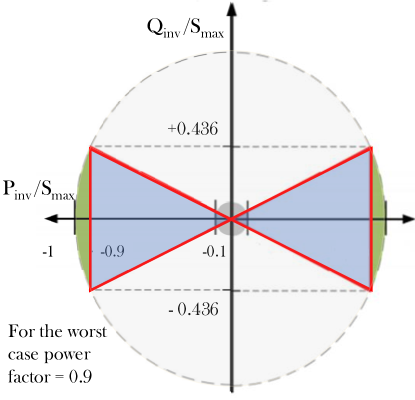
Figure 3: P, Q feasible region of inverter based on power factor limit of 0.9

Fig. 3 denotes the feasible active and reactive power regions based on the worst-case power factor limit. The blue-shaded and green regions are where the inverter is allowed to operate.

We next discuss the inverter rules for P(U) and Q(U) control, implemented at a faster timescale of one minute. The DSO imposes such control based on local voltage $U$. Many recent works such as [39, 40, 41, 42, 43] have explored similar volt-var (Q(U)) and volt-watt (P(U)) inverter control policy design. As standard, we consider inverter control to operate with P-priority, i.e., priority being given to active power output in case both P, Q set-points cannot be met.

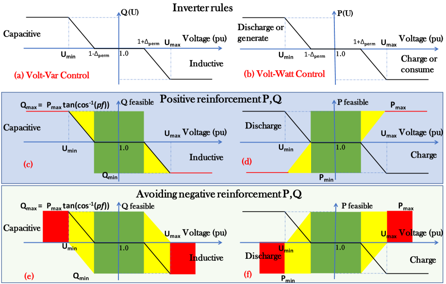
Figure 4: (a) Volt-var or Q(U) control and (b) volt-watt or P(U) translated into energy storage inverter feasible operation region considering positive reinforcement towards voltage regulation at the node denoted in the green region in (c) and (d). (e) and (f) denotes feasible region for avoiding negative reinforcement towards voltage regulation at the node. The feasible region is depicted as traffic-light control with green as no reduction in the feasible region, the yellow region shrinks the feasible region, and the red region shrinks it even further.

III-B Voltage zones for inverter control

Consider the instantaneous local voltage magnitude $U_{k_{i}}$ at PCC at time $k_{i}$. As shown in Fig. 4 (a) and (b), the operational voltage can be divided into 5 zones:

• Zone 1: $U_{k_{i}}<U_{\min}$,

• Zone 2: $U_{k_{i}}\in[U_{\min},1-\Delta_{perm})$,

• Zone 3: $U_{k_{i}}\in[1-\Delta_{perm},1+\Delta_{perm}]$,

• Zone 4: $U_{k_{i}}\in(1+\Delta_{perm},U_{\max}]$,

• Zone 5: $U_{k_{i}}>U_{\max}$,

where $\Delta_{perm}$ denotes the permissible voltage deviation in the distribution network before any voltage regulation is required. The values of $U_{\min}$, $U_{\max}$ are defined by the DSO. The value of $\Delta_{\text{perm}}$ will decide the droop slopes. For simplicity, we assume $\Delta_{\text{perm}}$ to be symmetrical around under and over-voltage.

The operating region for the inverter is defined based on the inverter’s characteristics and instantaneous voltage $U$. For active power, we denote the region as $R_{P}^{U}$, and for reactive power, as $R_{Q}^{U}$.

$$\begin{split}R_{P}^{U}(U_{k_{i}})\equiv[R^{U}_{P_{\min}},R^{U}_{P_{\max}}],\\ R_{Q}^{U}(U_{k_{i}})\equiv[R^{U}_{Q_{\min}},R^{U}_{Q_{\max}}],\end{split}$$ (7)

where $R^{U}_{P_{\min}}$, $R^{U}_{Q_{\min}}$ denote the lower operating envelopes and $R^{U}_{P_{\max}}$ and $R^{U}_{Q_{\max}}$ denote the upper operating envelopes. Note that these ranges are modified based on the zone that the voltage exists in and the kind of control. In the next sections III-C and III-D, we define three such control designs.

III-C PRC inverter operation

Under the Positive reinforcement control (PRC) model for P, Q, the inverter actively contributes to rectifying voltage issues in the different nodal voltage zones described in Section III-B. The ranges for P and Q under PRC are listed in Table III and depicted in Figs. 4 (c) and (d). For extreme nodal voltage levels (zones Z1 or Z5), the operating region is just one point. For moderate voltages (Z2 and Z4), the ranges for inverter output are restricted for voltage regulation using a linear droop. Finally, for voltage in Z3, inverter control does not limit arbitrage optimization opportunities.

TABLE III: Positive reinforcement inverter mode of operation

$U_{k_{i}}$	$[R^{U}_{P_{\min}},R^{U}_{P_{\max}}]$	$[R^{U}_{Q_{\min}},R^{U}_{Q_{\max}}]$
Z1	[$P_{\min}$, $P_{\min}$]	[$Q_{\max}$, $Q_{\max}$]
Z2	[$P_{\min}$, $\frac{P_{\min}(U_{k_{i}}-(1-\Delta_{\text{perm}}))}{U_{\min}-(1-\Delta_{\text{perm}})}$]	[$\frac{Q_{\max}(U_{k_{i}}-(1-\Delta_{\text{perm}}))}{U_{\min}-(1-\Delta_{\text{perm}})}$, $Q_{\max}$]
Z3	[$P_{\min}$, $P_{\max}$]	[$Q_{\min}$,$Q_{\max}$]
Z4	[$\frac{P_{\max}(U_{k_{i}}-(1+\Delta_{\text{perm}}))}{U_{\max}-(1+\Delta_{\text{perm}})}$, $P_{\max}$]	[$Q_{\min}$, $\frac{Q_{\min}(U_{k_{i}}-(1+\Delta_{\text{perm}}))}{U_{\max}-(1+\Delta_{\text{perm}})}$]
Z5	[$P_{\max}$, $P_{\max}$]	[$Q_{\min}$, $Q_{\min}$]

III-D ANRC inverter operation

Unlike PRC, avoiding negative reinforcement control (ANRC) model does not make the inverter actively contribute to mitigating voltage problems but prevents it from aggravating the current condition. The ranges for P and Q under ANRC are provided in Table  IV and Figs. 4 (e) and (f). Note that the $R^{U}$ for P, Q for ANRC is larger than or equal to the range generated using PRC, therefore, ANRC is less restrictive for prosumer energy optimization compared to PRC.

TABLE IV: ANRC inverter mode of operation

$U_{k_{i}}$	$[R^{U}_{P_{\min}},R^{U}_{P_{\max}}]$	$[R^{U}_{Q_{\min}},R^{U}_{Q_{\max}}]$
Z1	[$P_{\min}$, 0]	[0, $Q_{\max}$]
Z2	[$P_{\min}$, $\frac{P_{\max}(U_{\min}-U_{k_{i}})}{U_{\min}-(1-\Delta_{\text{perm}})}$]	[$\frac{Q_{\min}(U_{\min}-U_{k_{i}})}{U_{\min}-(1-\Delta_{\text{perm}})}$, $Q_{\max}$]
Z3	[$P_{\min}$, $P_{\max}$]	[$Q_{\min}$, $Q_{\max}$]
Z4	[$\frac{P_{\min}(U_{\max}-U_{k_{i}})}{U_{\max}-(1+\Delta_{\text{perm}})}$, $P_{\max}$]	[$Q_{\min}$, $\frac{Q_{\max}(U_{\max}-U_{k_{i}})}{U_{\max}-(1+\Delta_{\text{perm}})}$]
Z5	[0, $P_{\max}$]	[$Q_{\min}$, 0]

III-E Hybrid inverter operation

From Fig. 4, we observe that PRC is more restrictive for active and reactive power control compared to ANRC. Typically, energy management in low voltage consumers deals with only active power, therefore, PRC-based inverter P control can lead to a significant reduction in benefits for prosumer energy optimization. We propose a hybrid inverter control policy that selects active power output based on ANRC and reactive power output based on PRC. The lower and upper bound of ranges for this based on voltage magnitude is listed in Table V.

TABLE V: Hybrid inverter mode of operation

$U_{k_{i}}$	$[R^{U}_{P_{\min}},R^{U}_{P_{\max}}]$	$[R^{U}_{Q_{\min}},R^{U}_{Q_{\max}}]$
Z1	[$P_{\min}$, 0]	[$Q_{\max}$, $Q_{\max}$]
Z2	[$P_{\min}$, $\frac{P_{\max}(U_{\min}-U_{k_{i}})}{U_{\min}-(1-\Delta_{\text{perm}})}$]	[$\frac{Q_{\max}(U_{k_{i}}-(1-\Delta_{\text{perm}}))}{U_{\min}-(1-\Delta_{\text{perm}})}$, $Q_{\max}$]
Z3	[$P_{\min}$, $P_{\max}$]	[$Q_{\min}$, $Q_{\max}$]
Z4	[$\frac{P_{\min}(U_{\max}-U_{k_{i}})}{U_{\max}-(1+\Delta_{\text{perm}})}$, $P_{\max}$]	[$Q_{\min}$, $\frac{Q_{\min}(U_{k_{i}}-(1+\Delta_{\text{perm}}))}{U_{\max}-(1+\Delta_{\text{perm}})}$]
Z5	[0, $P_{\max}$]	[$Q_{\min}$, $Q_{\min}$]

III-F Minimizing Constraint validation

From (5), solving $P_{LP}$ (energy arbitrage) without any inverter control gives $P_{inv}^{k_{i}}=P^{i}_{inv}=f(x_{i})-r_{i}$ with $P_{\text{curt}}^{k_{i}}=0$, and $Q_{inv}^{k_{i}}=Q_{\text{default}}=0~{}\forall~{}k_{i}$. Under the permissible active P(U) and reactive limits Q(U) defined under PRC, ANRC, or hybrid control, the following three conditions may emerge:

• $P^{i}_{inv}$ satisfies both the output constraints derived by P(U) and Q(U) curves,

• $P^{i}_{inv}$ satisfies only one of the output constraints derived by P(U) or Q(U),

• $P^{i}_{inv}$ does not satisfy both output constraints derived by P(U) and Q(U) curves.

For cases where the output $P^{i}_{inv}$ lies outside the feasible range $[R^{U}_{P_{\min}},R^{U}_{P_{\max}}]$ of voltage-based operation, let the nearest boundary to $P^{i}_{inv}$ be $P^{U}_{trgt}$. The controller solves the following linear programming optimization problem ($P_{LP}^{curt}$) to determine minimum curtailment of $r_{i}$ to reach $P^{U}_{trgt}$:

$$(P_{LP}^{curt})~{}~{}\min_{P_{B}^{k_{i}}}~{}~{} P_{\text{curt}}^{k_{i}}$$ (8a)

s.t. $$P_{B}^{k_{i}}-(r_{i}-P_{\text{curt}}^{k_{i}})=P^{U}_{trgt}$$ (8b)

$$0\leq P_{\text{curt}}^{k_{i}}\leq r_{i},$$ (8c)

$$P_{B}^{k_{i}}\in\Big{[}\max\Big{(}\delta_{\min},\frac{(b_{\min}-b_{k-1})\eta_{\text{dis}}}{k}\Big{)},$$

$$\hskip 30.0pt\min\Big{(}{\delta_{\max}},\frac{(b_{\max}-b_{k-1})}{k\eta_{\text{ch}}}\Big{)}\Big{]}.$$ (8d)

Here, $P^{U}_{trgt}$ is based on the corresponding zone in Tables III, IV, or V and voltage $U_{k_{i}}$. Note that in some cases, ($P_{LP}^{curt}$) may not have a feasible solution due to too low or high state of charge of the battery, high renewable generation, or limited feasible range of operation for the inverter. In that case, $P_{\text{curt}}^{k_{i}}$ and $P_{B}^{k_{i}}$ are operated based on sign of $P^{U}_{trgt}$, i.e., if $P^{U}_{trgt}>0$ then charge the battery at $P_{B}^{\max^{k_{i}}}$, else discharge at $P_{B}^{\min^{k_{i}}}$. If $P^{U}_{trgt}>0$ then $P_{\text{curt}}^{k_{i}}$ is set at $r_{i}$, else it is set to $0$. The inverter’s remaining capacity is then utilized to set the reactive power. In case the remaining capacity is not enough, the reactive power is set closest to the minimum or maximum bound level based on Tables III, IV, or V. The inverter control procedure is detailed in Appendix -B.

Algorithm 1 details the entire procedure, conducted in a receding horizon fashion. Here the energy arbitrage is first solved using $(P_{LP})$ at Step 4 to give battery states at a slower timescale. Then the voltage is regulated based on inverter rules at a faster timescale for each time slot. First, the inverter rules for selected permissible P and Q ranges are identified in Step 10. Then the curtailed active power and reactive injection are determined using the associated Algorithm 2, detailed in Appendix -B. The battery’s initial state for the next 15 minutes is fixed based on the battery charge level at the end of the faster timescale.

Inputs: $U_{k_{i}},r_{i},b_{0},S_{\max}$, battery parameters

1:Set $P_{\max}=S_{\max}$, $i=1$

2:while $i<=N$ do

3:    Based on battery parameters, price levels, inelastic load, flexible load, renewable generation, initial battery level calculated matrices $A,b,X,f,lb,ub,$ detailed in Appendix -A,

4:    Solve $P_{LP}$ using load, generation, electricity price values, and initial battery capacity,

5:    Set $k=0$

6:    while $k<15$ do

7:         Increment $k=k+1$,

8:         Inverter output based on energy management $\zeta_{i}=f(x_{i})-r_{i}$,

9:         Measure local voltage $U_{k_{i}}$,

10:         Based on $U_{k_{i}}$ calculate $R^{U}_{P_{\min}},R^{U}_{P_{\max}},R^{U}_{Q_{\min}},R^{U}_{Q_{\max}}$ as global variables. Refer to Table III for PRC, Table IV for ANRC and Table V for hybrid inverter control,

11:         Calculate $Q_{\max}$ based on (6b) as a function of $R_{P}^{U}$

12:         Execute Algorithm 2 with range derived from Tables III, IV, or V to find $P_{\text{curt}}^{k_{i}},P_{\text{inv}}^{k_{i}},Q_{\text{inv}}^{k_{i}}$,

13:         Update battery charge level $b_{k_{i}}=b_{{k-1}_{i}}+f^{-1}(P_{B}^{k_{i}})$

14:         Concatenate results $P_{\text{curt}},P_{\text{inv}},Q_{\text{inv}},b_{{k=15}_{i}}$.

15:    end while

16:    Update battery charge level $b_{i}=b_{{k=15}_{i}}$

17:    Increment $i=i+1$,

18:    Calculate matrices $A,b,X,f,lb,ub$ for time $i$ till $N$

19:end while

20:Return $P_{\text{curt}},P_{\text{inv}},Q_{\text{inv}}$.

Algorithm 1 Prosumer energy management with inverter rules

In the next section, we describe methods to understand the effect of location on the prosumer operation, while imposing the inverter controls with arbitrage.

IV Effect of prosumer location on DN feeder

In this section, we develop performance indices for understanding the effect of prosumer location in a DN on its optimization for arbitrage, with rules for DN voltage correction, and the effect of PRC, ANRC, or hybrid voltage control policies.

IV-A Performance indices

The proposed indices relate to (a) voltage violations (b) arbitrage gains (c) energy curtailment [44, 19], all of which are very relevant to operational issues in the distribution grid as well as understanding the extent of profitability and opportunity cost associated with inverter interfaced resources in the distribution grids. In fact, the comparison of arbitrage profits versus issues of grid limits on voltage is the primary objective of study for several smart grid control/optimization algorithms proposed in the literature as mentioned in [45].

We consider the following performance indices:
Prosumer energy bill: If inverter rules and associated control are imposed on prosumers, their savings due to the operation of the battery will be reduced due to voltage fluctuations, with more loss at nodes with greater fluctuation of voltage such as terminal nodes. Note that the cost of consumption without inverter control at node $j$ is denoted as

$$C_{\text{wic}}^{j}=\sum_{i}\Big{(}p_{b}^{i}(d_{i}+y_{i}-r_{i}+f(x_{i}))^{+}-p_{s}^{i}(d_{i}+y_{i}-r_{i}+f(x_{i}))^{-}\Big{)}h.$$ (9)

The cost of consumption with inverter control for a prosumer connected at node $j$ is denoted as

$$C_{\text{inv}}^{j}=\sum_{i}^{N} p_{b}^{i}\big{(}d_{i}+y_{i}-r_{i}+\frac{1}{15}\sum_{k=1}^{15}(P_{B}^{k_{i}}+P_{\text{curt}}^{k_{i}})\big{)}^{+}h$$

$$- p_{s}^{i}\big{(}d_{i}+y_{i}-r_{i}+\frac{1}{15}\sum_{k=1}^{15}(P_{B}^{k_{i}}+P_{\text{curt}}^{k_{i}})\big{)}^{-}h.$$ (10)

The loss of consumer gain (LCG) due to location is denoted as

$$\text{LCG}_{j}=C_{\text{inv}}^{j}-C_{\text{wic}}^{j}.$$ (11)

Prosumer energy curtailed: Nodes with greater voltage fluctuations result in a more restricted range of inverter operation, thus leading to greater energy curtailment. The total curtailed energy (TCE) for inverter at node $j$ is denoted as

$$\text{TCE}_{j}=\sum_{k}P_{\text{curt}}^{(j,k)}.$$ (12)

Prosumer voltage correction: The Voltage correction index (VCI) consists of four metrics that shows

• cumulative instances where voltage is beyond $V_{\max}$,

• cumulative instances where voltage is beyond $1+\Delta_{\text{perm}}$,

• cumulative instances where voltage is below $1-\Delta_{\text{perm}}$,

• cumulative instances where voltage is below $V_{\min}$.

VCI for voltage time series $U$ is given as

$$\begin{split}\text{VCI}(U)=\Big{[}\sum_{k}\mathbf{1}(U>U_{\max}),~{}~{}\sum_{k}\mathbf{1}(U>1+\Delta_{\text{perm}}),\\ \sum_{k}\mathbf{1}(U<1-\Delta_{\text{perm}}),\sum_{k}\mathbf{1}(U<U_{\min})\Big{]},\end{split}$$ (13)

where $\mathbf{1}(\text{condition})$ returns 1 if the condition is true, else it returns 0. VCI provides the number of samples where the voltage level is outside the permissible level. The cumulative voltage correction can be identified by adding all voltage deviation outside $[1-\Delta_{\text{perm}},1+\Delta_{\text{perm}}]$ denoted as cumulative voltage correction (CVC). CVC for voltage U is given as

$$\begin{split}\text{CVC}(U)=\sum_{k}\mathbf{1}(U>1+\Delta_{\text{perm}})(U-1-\Delta_{\text{perm}})~{}+\\ \sum_{k}\mathbf{1}(U<1-\Delta_{\text{perm}})(1-\Delta_{\text{perm}}-U).\end{split}$$ (14)

Next, we use the performance indices proposed to quantify the locational impact on prosumer energy optimization in presence of inverter rules based on voltage measurement at PCC.

V Numerical results

Three numerical simulations are presented in this section. In Section V-A, energy optimization presented in Section II is implemented. The second numerical experiment in Section V-B combines the energy optimization with inverter P(U) and Q(U) rules for a prosumer. The effect of two controls PRC and ANRC with varying inverter sizes on performance indices are presented. Based on historical voltage variation, this exercise can be used to select the best-suited inverter. The DN locational dependency of prosumer inverter control is explored in Section V-C. A stylized DN with 3 identical consumers at different positions in the distribution feeder is analyzed for (a) their cost of energy consumption, (b) voltage correction ability, and (c) renewable energy curtailment. Performance indices presented in Section IV are used to compare different cases.

V-A Energy optimization of storage and load flexibility

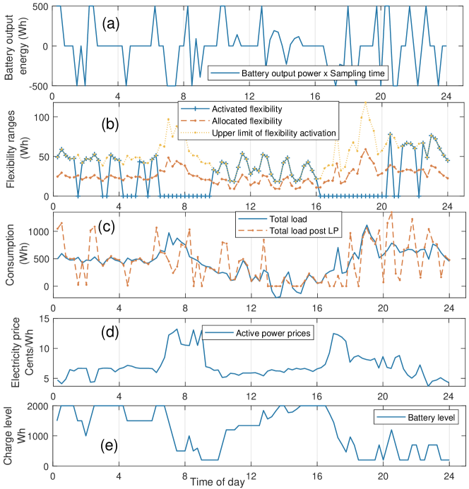
Figure 5: Numerical validation for activating load flexibility and energy storage arbitrage; 5% load flexibility, $p_{s}/p_{b}=0.5$

The results for energy management with 5% load flexibility, 2 kWh 1C-1C battery, 1.8 kWp solar is presented in Fig. 5. Electricity price data is used from New York Independent System Operator or NYISO wholesale real-time electricity price. The load flexibility bounds are from 0 to twice the available flexibility. The deadline constraint ensures that the energy consumption of the flexible resources is respected. Fig. 5 (a) shows the battery ramp rate, (b) the operation and bounds of load flexibility, (c) the total billable load, (d) buying price of electricity, and (e) the battery charge level. The flexible load output shows that it is activated in a way to avoid morning and evening peaks in electricity prices, thus reducing the cost of consumption. Since $\kappa=0.5$, self-consumption is prioritized which is evident from Fig. 5 (c) where the net load after energy optimization saturates at zero, therefore, avoiding injection of active power in DN.

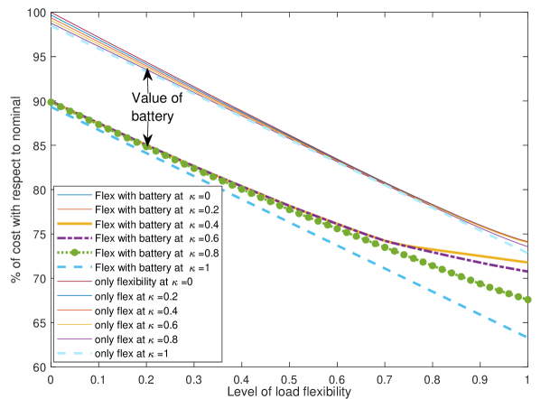
Figure 6: Value of storage, flexibility with varying load flexibility levels and $\kappa$ which is the ratio of selling price and buying price of electricity

Fig. 6 shows the decrease in the cost of consumption with load flexibility without and with battery. Prosumers can reduce their cost of consumption by more than 25% by selecting a consumption profile without reducing energy consumption. Observe that load flexibility control is immune to $\kappa=p_{s}/p_{b}$. However, for batteries, the "value of battery" is higher for a lower value of $\kappa$.

V-B Inverter controls with(out) energy optimization

Residential bidirectional inverters interfacing solar PV and battery are expensive components. Selecting the size of the inverter is crucial in limiting the solar curtailed energy. In this numerical simulation, we perform a sensitivity analysis using (a) percentage solar energy, (b) percentage cost of consumption with respect to nominal load profile, and (c) percentage of profit with respect to only energy optimization without voltage control. Many DSOs motivate prosumers to self-consume their PV generation, this is ensured by setting $p_{s}<<p_{b}$. For this experiment, we assume $p_{s}=0$. The size of the solar panel is 2kWp and the battery capacity is 2 kWh (0.5C-0.5C, $\eta_{ch}=\eta_{dis}=0.95$) requires $\approx$1.25 kW inverter for PRC inverter control and close to $\approx$2 kW for ANRC inverter control. Note from Fig. 7 that the profit with ANRC approaches to energy optimization profit for a large-sized inverter. Fig. 7 also shows that for PV and battery, sharing an inverter will lead to a reduction in the required size of inverters compared to if individual inverters are used for PV and battery. For the oversized inverter, the profit with ANRC reaches 82.4% and PRC reaches 25% compared to only energy optimization.

Clearly, PRC-based inverter control will drastically reduce the energy optimization opportunities for a prosumer. Thus, it is anticipated that more volatile nodes at the end of a radial distribution feeder may have to pay more for energy compared to the same amount of energy consumed close to the substation, causing the locational disparity. In Section V-C we quantify this locational disparity.

TABLE VI: Line parameters for the network considered

branch from & to node	Resistance ($\Omega$)	Reactance ($\Omega$)
node 1 to 2	0.0922	0.0470
node 2 to 3	0.1844	0.0940
node 3 to 4	0.3660	0.1864

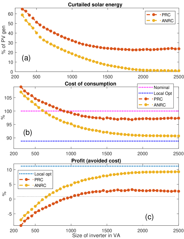
Figure 7: Inverter size impact on DG curtailed and consumer bill with $\kappa=1$

V-C Effect of prosumer location in radial DN

DN feeders are predominantly radial. These feeders are exposed to different levels of voltage fluctuations depending on their location on the feeder. For nodes close to the feeder, the fluctuation is small compared to node buses away from the feeder. We consider 4 bus simple distribution feeders. The network diagram is shown in Fig. 8. The line parameters of the 4 bus network considered in this work are listed in Table VI. The minimum and maximum voltage are assumed to be $V_{\min}=0.92$ and $V_{\max}=1.08$. The permissible voltage level $\Delta_{\text{perm}}=0.04$. For this numerical example, the inverter is oversized so as to not curtail energy due to the capacity limitation of the inverter. The PV size at the prosumer end is 2.5 KWp and a 1 kW 0.5C-0.5C battery is connected to the 3 kVA bidirectional inverter.

The loads at nodes 2, 3, and 4 consist of a residential prosumer with identical load and solar generation. Energy optimization with/without voltage-based inverter control is implemented at one node at a time. The nodal voltage in absence of inverter control is shown in Fig. 9. The voltage at node 2 shows minimal fluctuations compared to node 4. The following controls are evaluated and listed in Table VII:

• Prosumer with no energy optimization,

• Energy optimization without inverter rules,

• Energy optimization with P(U) and Q(U) for ANRC,

• Energy optimization with P(U) and Q(U) for PRC,

• Energy optimization with hybrid policy: P control using ANRC and Q based on PRC.

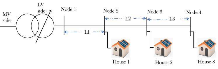
Figure 8: Stylized 4 bus radial DN with identical prosumers connected at bus 2,3,4

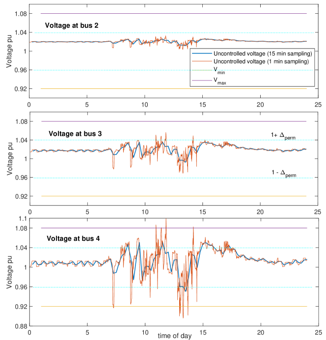
Figure 9: Nodal voltage in 3 bus radial distribution feeder

TABLE VII: Effect of inverter control on performance indices

Mode		Nominal case			With inverter control
		(with energy opt.)			PRC			ANRC			Hybrid
Node id		2	3	4	2	3	4	2	3	4	2	3	4
VCI	$\sum\mathbf{1}(V>V_{\max})$	0	0	4	0	0	0	0	0	0	0	0	0
	$\sum\mathbf{1}(V>1+\Delta_{\text{perm}})$	0	3	86	0	3	0	0	3	82	0	3	71
	$\sum\mathbf{1}(V<1-\Delta_{\text{perm}})$	0	0	39	0	0	48	0	0	35	0	0	35
	$\sum\mathbf{1}(V<V_{\min})$	0	0	1	0	0	0	0	0	1	0	0	0
CVC		0	0.006	1.71	0	0.006	0.637	0	0.006	1.345	0	0.006	0.329
Consumption cost (€ cents)		37.78	37.78	37.78	37.78	38.14	54.16	37.78	37.78	38.27	37.78	37.78	38.27
LCG (%)		-	-	-	0%	0.95%	43.35%	0%	0%	1.3%	0%	0%	1.3%
TCE (kWh)		0	0	0	0	0.102	2.275	0	0	0.188	0	0	0.188

Table VII summarizes the results. The nodal voltages are calculated using power flows performed using MATPOWER [46]. Since the nodal voltage control is performed in an open loop, therefore, we observe the voltage deterioration for some time instances due to energy optimization, although the correction is performed for cases where voltage is outside its bound. The prosumer connected at node 4 has LCG increases up to 43.35%, refer to Table VII, causing increased consumption cost. For ANRC, the curtailed energy is significantly reduced compared to PRC inverter control. ANRC does correct the node voltage, however, the correction is lower compared to PRC. ANRC is more favorable for consumer optimization as LCG is reduced from 43.35% for PRC to a mere 1.3%. Using ANRC will be fairer for prosumers located away from the feeder. Note that for only energy optimization at node 4, the voltage profile deteriorates the most. This implies prosumer energy optimization needs to consider the network state into account.

For the prosumer located at node 2, the local voltage is always within bounds due to its proximity to the DN substation. Therefore, the prosumer does not have to bear any loss in energy optimization due to inverter rules and also does not have to provide any Q. This is also observed in [47]. One could observe that a prosumer connected at node 4 is at a disadvantage due to its location in the network and is obliged to supply Q and limit energy optimization gains without receiving any additional benefits compared to a prosumer at node 2.

The hybrid inverter control uses ANRC for active power control and uses PRC for reactive power control. For our network example, R/X = 2. The hybrid inverter control outperforms only PRC in terms of CVC. For the hybrid model, CVC at node 4 is 0.3286 compared to 0.637 for PRC. Fig. 10 compares the voltages with only prosumer energy optimization and with energy optimization plus inverter voltage control.

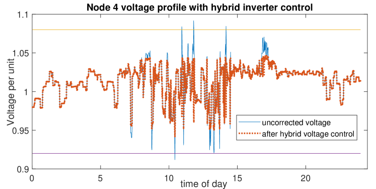
Figure 10: Corrected voltage at node 4 for hybrid controller

For the simulations, the computation time is calculated using 10000 Monte Carlo simulation runs. Simulations are performed on HP Intel(R) Core(TM) i7 CPU, 1.90GHz, 32 Gb RAM personal computer on Matlab 2021a. The runtime evaluations for energy arbitrage based on LP (see Fig. 11(a)) is done separately from run times for voltage regulation in the inner loop (see Fig. 11(b)). Note that the mean runtime for energy arbitrage is higher than the meantime of the inner loop with 1 iteration of energy arbitrage every 15 minutes because of the shrinking time horizon and because arbitrage is performed only once for the next 15 minutes. Key observations for runtime are

• LP-based energy arbitrage takes on average 0.0168 seconds for running 96 times for the entire day.

• The inner loop which performs voltage regulation includes (a) time taken to perform Power flows that depend on the network size, (b) one iteration of energy arbitrage every 15 minutes, and (c) voltage regulation performed every minute. For the test network, 1440 power flows are performed for 1 day, each iteration on average takes 0.015 seconds.

• The total runtime for energy arbitrage, power flows, and voltage regulation takes on an average of 20.55 seconds. Monte Carlo simulations for 1000 days were performed.

Thus, the proposed voltage regulation with local energy optimization is computationally efficient.

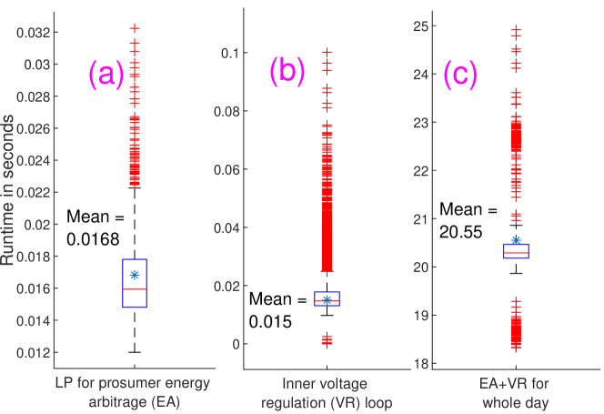
Figure 11: Computational time taken for energy arbitrage and voltage regulation for 10000 Monte Carlo runs. (a) energy arbitrage based on LP for one entire day, (b) Inner loop runtime with 1 iteration of LP for energy arbitrage in receding horizon, (c) Total runtime for local energy optimization with voltage regulation for the entire day. The blue star shows the mean value.

VI Conclusion and discussion

We propose an LP formulation to control energy storage and load flexibility while considering electricity price variation, load profile, and renewable generation over a time horizon. This optimization is performed at a slower timescale. The output of local energy optimization is taken as input to update inverter output based on grid rules for inverter output on the basis of local voltage measurement. The P(U) and Q(U) inverter control is translated into positive reinforcement control (PRC) and avoiding negative reinforcement control (ANRC). The inverter control is performed at a finer timescale. Algorithms are presented to consider these different time scales, inverter size, locally measured voltage, and myopic curtailment reduction.

We quantify the prosumer "loss of consumer gain" due to their location. A stylized network-based analysis is performed for a radial distribution network. Numerical results for a DN feeder indicate the prosumer connected at the end of the feeder may have to pay 43% more than prosumers close to the feeder. DSOs and regulators should hence consider that prosumer location could cause a disparity in their cost of consumption. Hybrid inverter control with P control using ANRC and Q control using PRC along with P-priority significantly reduces the disparity for prosumers located at more vulnerable nodes while significantly improving the nodal voltage. This control methodology can be utilized to minimize the locational disparity caused by voltage-based inverter control from a prosumer perspective.

Inverter sizing is crucial for ensuring the full use of local resources such as energy storage, PV generation, and network connection rules. We observe through numerical results that bidirectional inverter architecture where residential renewable generation and battery share a single inverter could lead to a significant reduction in its size compared to dedicated solar and battery inverters.

The mapping of voltage into P, and Q feasible ranges can be utilized in active distribution network design while using these ranges for cost optimization. Future work will utilize a forecast of nodal voltages for real-time operation and analyze the impact of inverter control on feeder hosting capacity. Further assessment is required to optimally set and numerically verify convergence of the droop slopes for envelope generation while taking into account the location of a prosumer in the DN. Finally, we will compare the centralized dispatch of resources for voltage regulation with our proposed distributed framework developed in this work.

-A LP formulation for arbitrage with energy storage and price-based flexibility dispatch

In our earlier work [36], we used linear programming (LP) based formulation to solve the optimal energy storage arbitrage problem. This LP formulation uses epigraph-based minimization [48]. We extend the LP formulation in [36, 49] for including control of flexible load under time-varying electricity price. The formulation in [36] uses the geometry of the cost function to form 4 line segments over which the epigraph-based cost function is minimized. Since flexible load $y_{i}\geq 0$, the operation of flexible loads does not lead to adding more line segments to the geometry of the cost function in [36, 49]. The LP formulation for solving the arbitrage problem is given as $P_{LP}$. The objective function and associated linear constraints are given in (15).

$$(P_{LP})~{}~{}\min\quad\{t_{1}+t_{2}+...+t_{N}\},$$ (15a)

subject to,

$$\text{Segment 1:~{}}\frac{p_{b}^{i}}{\eta_{ch}}x_{i}+p_{b}^{i}y_{i}-t_{i}\leq-z_{i}p_{b}^{i},~{}\forall~{}i,$$ (15b)

$$\text{Segment 2:~{}}{p_{s}^{i}}{\eta_{dis}}x_{i}+p_{s}^{i}y_{i}-t_{i}\leq-z_{i}p_{s}^{i},~{}\forall~{}i,$$ (15c)

$$\text{Segment 3:~{}}{p_{b}^{i}}{\eta_{dis}}x_{i}+p_{b}^{i}y_{i}-t_{i}\leq-z_{i}p_{b}^{i},~{}\forall~{}i,$$ (15d)

$$\text{Segment 4:~{}}\frac{p_{s}^{i}}{\eta_{ch}}x_{i}+p_{s}^{i}y_{i}-t_{i}\leq-z_{i}p_{s}^{i},~{}\forall~{}i,$$ (15e)

$$\text{Ramp constraint:~{}}x_{i}\in[X_{\min},X_{\max}],~{}\forall~{}i,$$ (15f)

$$\text{Capacity constraint:~{}}\sum{x_{i}}\in[b_{\min}-b_{0},b_{\max}-b_{0}],~{}\forall~{}i,$$ (15g)

$$\text{Flexibility ramp constraint:~{}}\sum{y_{i}}\in[y_{\min}^{i},y_{\max}^{i}],~{}\forall~{}i,$$ (15h)

$$\text{Cumulative flexibility:}\sum{y_{i}}\in[K-\epsilon,K+\epsilon],\text{for~{}}i=N.$$ (15i)

The matrix format for the optimization problem $P_{LP}$ is denoted as minimize ${f}^{T}X$, subject to ${A}X\leq b$, and $X\in[lb,ub]$. The dimension of $A$ is (6N+2)x3N, $b$ is (6N+2)x1, $X$ and $f$ are of size 3Nx1, and N denotes the number of samples in the horizon of optimization.

$$f\text{=}{\begin{bmatrix}0\\ :\\ 0\\ 0\\ :\\ 0\\ 1\\ :\\ 1\\ \end{bmatrix}},X\text{=}{\begin{bmatrix}x_{1}\\ :\\ x_{N}\\ y_{1}\\ :\\ y_{N}\\ t_{1}\\ :\\ t_{N}\\ \end{bmatrix}},$$ (16)

$$lb\text{=}{\begin{bmatrix}X_{\min}\\ X_{\min}\\ :\\ X_{\min}\\ y_{\min}(1)\\ y_{\min}(2)\\ :\\ y_{\min}(N)\\ T_{\min}\\ T_{\min}\\ :\\ T_{\min}\\ \end{bmatrix}}\leq{\begin{bmatrix}x_{1}\\ x_{2}\\ :\\ x_{N}\\ y_{1}\\ y_{2}\\ :\\ y_{N}\\ t_{1}\\ t_{2}\\ :\\ t_{N}\\ \end{bmatrix}}\leq ub\text{=}{\begin{bmatrix}X_{\max}\\ X_{\max}\\ :\\ X_{\max}\\ y_{\max}(1)\\ y_{\max}(2)\\ :\\ y_{\max}(N)\\ T_{\max}\\ T_{\max}\\ :\\ T_{\max}\\ \end{bmatrix}},~{}{b}={\begin{bmatrix}-z_{i}p_{b}(1)\\ :\\ -z_{i}p_{b}(N)\\ -z_{i}p_{s}(1)\\ :\\ -z_{i}p_{s}(N)\\ -z_{i}p_{s}(1)\\ :\\ -z_{i}p_{s}(N)\\ -z_{i}p_{b}(1)\\ :\\ -z_{i}p_{b}(N)\\ b_{\max}-b_{0}\\ :\\ b_{\max}-b_{0}\\ b_{0}-b_{\min}\\ :\\ b_{0}-b_{\min}\\ K+\epsilon\\ -K+\epsilon\end{bmatrix}}.$$ (17)

where $T_{\min}$ and $T_{\max}$ are bounds on $t_{i}$. Since these bounds are not known to us, we choose $T_{\min}$ to be negative with a large magnitude and $T_{\max}$ to be positive with a large magnitude.

$${A}={\left[\begin{array}[]{c c c c c|c c c c c|c c c c c}\frac{p_{b}(1)}{\eta_{ch}}&0&0&...&0&p_{b}(1)&0&0&...&0&-1&0&0&...&0\\ 0&\frac{p_{b}(2)}{\eta_{ch}}&0&...&0&0&p_{b}(2)&0&...&0&0&-1&0&...&0\\ :&:&:&...&:&:&:&:&...&:&:&:&:&...&:\\ 0&0&0&...&\frac{p_{b}(N)}{\eta_{ch}}&0&0&0&...&p_{b}(N)&0&0&0&...&-1\\ \hline\cr{p_{s}(1)}{\eta_{dis}}&0&0&...&0&p_{s}(1)&0&0&...&0&-1&0&0&...&0\\ 0&{p_{s}(2)}{\eta_{dis}}&0&...&0&0&p_{s}(2)&0&...&0&0&-1&0&...&0\\ :&:&:&...&:&:&:&:&...&:&:&:&:&...&:\\ 0&0&0&...&{p_{s}(N)}{\eta_{dis}}&0&0&0&...&p_{s}(N)&0&0&0&...&-1\\ \hline\cr\frac{p_{s}(1)}{\eta_{ch}}&0&0&...&0&p_{s}(1)&0&0&...&0&-1&0&0&...&0\\ 0&\frac{p_{s}(2)}{\eta_{ch}}&0&...&0&0&p_{s}(2)&0&...&0&0&-1&0&...&0\\ :&:&:&...&:&:&:&:&...&:&:&:&:&...&:\\ 0&0&0&...&\frac{p_{s}(N)}{\eta_{ch}}&0&0&0&...&p_{s}(N)&0&0&0&...&-1\\ \hline\cr{p_{b}(1)}{\eta_{dis}}&0&0&...&0&p_{b}(1)&0&0&...&0&-1&0&0&...&0\\ 0&{p_{b}(2)}{\eta_{dis}}&0&...&0&0&p_{b}(2)&0&...&0&0&-1&0&...&0\\ :&:&:&...&:&:&:&:&...&:&:&:&:&...&:\\ 0&0&0&...&{p_{b}(N)}{\eta_{dis}}&0&0&0&...&p_{b}(N)&0&0&0&...&-1\\ \hline\cr 1&0&0&...&0&0&0&0&...&0&0&0&0&...&0\\ 1&1&0&...&0&0&0&0&...&0&0&0&0&...&0\\ :&:&:&...&:&:&:&:&...&:&:&:&:&...&:\\ 1&1&1&...&1&0&0&0&...&0&0&0&0&...&0\\ \hline\cr-1&0&0&...&0&0&0&0&...&0&0&0&0&...&0\\ -1&-1&0&...&0&0&0&0&...&0&0&0&0&...&0\\ :&:&:&...&:&:&:&:&...&:&:&:&:&...&:\\ -1&-1&-1&...&-1&0&0&0&...&0&0&0&0&...&0\\ \hline\cr 0&0&0&...&0&1&1&1&...&1&0&0&0&...&0\\ 0&0&0&...&0&-1&-1&-1&...&-1&0&0&0&...&0\end{array}\right]},$$ (18)

-B LP formulation for arbitrage with energy storage and price-based flexibility dispatch

We provide here, the details of the algorithm to determine curtailment, inverter active and reactive outputs over a faster timescale, discussed in Section III-F. Algorithm 2 used bounds $[R^{U}_{P_{\min}},R^{U}_{P_{\max}}]$ and $[R^{U}_{Q_{\min}},R^{U}_{Q_{\max}}]$ from the respective Tables III, IV, and V for different control policies (PRC, ANRC or Hybrid).

1:Use $f(x_{i}),r_{i}$ as global variables,

2:if $\zeta_{i}\in[R^{U}_{P_{\min}},R^{U}_{P_{\max}}]$ and $Q_{\text{default}}\in[R^{U}_{Q_{\min}},R^{U}_{Q_{\max}}]$ then

3:     Set $P_{\text{inv}}^{k_{i}}=\zeta_{i},Q_{\text{inv}}^{k_{i}}=0,P_{\text{curt}}^{k_{i}}=0$

4:else if $\zeta_{i}\notin[R^{U}_{P_{\min}},R^{U}_{P_{\max}}]$ and $Q_{\text{default}}\in[R^{U}_{Q_{\min}},R^{U}_{Q_{\max}}]$ then

5:     if $\zeta_{i}<R^{U}_{P_{\min}}$ then Active_Point_Minimize($R^{U}_{P_{\min}}$)

6:     else if $\zeta_{i}>R^{U}_{P_{\max}}$ then Active_Point_Minimize($R^{U}_{P_{\max}}$)

7:     end if

8:     Set $Q_{\text{inv}}^{k_{i}}=0$

9:else if $\zeta_{i}\in[R^{U}_{P_{\min}},R^{U}_{P_{\max}}]$ & $Q_{\text{default}}\notin[R^{U}_{Q_{\min}},R^{U}_{Q_{\max}}]$ then

10:     if $Q_{\text{default}}<R^{U}_{Q_{\min}}$ then     $Q_{\text{inv}}^{k_{i}}=R^{U}_{Q_{\min}}$

11:     else if $Q_{\text{default}}>R^{U}_{Q_{\max}}$ then    $Q_{\text{inv}}^{k_{i}}=R^{U}_{Q_{\max}}$

12:     end if

13:     Set $P_{\text{inv}}^{k_{i}}=\zeta_{i},P_{\text{curt}}^{k_{i}}=0$

14:else if $\zeta_{i}\notin[R^{U}_{P_{\min}},R^{U}_{P_{\max}}]$ & $Q_{\text{default}}\notin[R^{U}_{Q_{\min}},R^{U}_{Q_{\max}}]$ then

15:     if $\zeta_{i}<R^{U}_{P_{\min}}$ and $Q_{\text{default}}<R^{U}_{Q_{\min}}$ then

16:         Execute Active_Point_Minimize($R^{U}_{P_{\min}}$) to find $P_{\text{curt}}^{k_{i}},P_{\text{inv}}^{k_{i}}$; Set $Q_{\text{inv}}^{k_{i}}=R^{U}_{Q_{\min}}$,

17:     else if $\zeta_{i}<R^{U}_{P_{\min}}$ and $Q_{\text{default}}>R^{U}_{Q_{\max}}$ then

18:         Execute Active_Point_Minimize($R^{U}_{P_{\min}}$) to find $P_{\text{curt}}^{k_{i}},P_{\text{inv}}^{k_{i}}$; Set $Q_{\text{inv}}^{k_{i}}=R^{U}_{Q_{\max}}$,

19:     else if $\zeta_{i}>R^{U}_{P_{\max}}$ and $Q_{\text{default}}<R^{U}_{Q_{\min}}$ then

20:         Execute Active_Point_Minimize($R^{U}_{P_{\max}}$) to find $P_{\text{curt}}^{k_{i}},P_{\text{inv}}^{k_{i}}$; Set $Q_{\text{inv}}^{k_{i}}=R^{U}_{Q_{\min}}$,

21:     else if $\zeta_{i}>R^{U}_{P_{\max}}$ and $Q_{\text{default}}>R^{U}_{Q_{\max}}$ then

22:         Execute Active_Point_Minimize($R^{U}_{P_{\max}}$) for $P_{\text{curt}}^{k_{i}},P_{\text{inv}}^{k_{i}}$, and Set $Q_{\text{inv}}^{k_{i}}=R^{U}_{Q_{\max}}$,

23:     end if

24:end if

25:return $P_{\text{curt}}^{k_{i}},P_{\text{inv}}^{k_{i}},Q_{\text{inv}}^{k_{i}}$

26:function Active_Point_Minimize($P^{U}_{trgt}$)

27:     minimize $P_{\text{curt}}^{k_{i}}$ as described in (8), and Set $P_{\text{inv}}^{k_{i}}=P_{B}^{k_{i}}-r_{i}+P_{\text{curt}}^{k_{i}}$,

28:     if optimization ($P_{LP}^{curt}$) does not provide a solution then

29:         if $P^{U}_{trgt}>0$ then $P_{\text{curt}}^{k_{i}}=r_{i}$ and $P_{B}^{k_{i}}=$ max charge,

30:         else if $P^{U}_{trgt}<0$ then $P_{\text{curt}}^{k_{i}}=0$ and $P_{B}^{k_{i}}=$ max discharge,

31:         end if

32:     end if

33:     return $P_{\text{curt}}^{k_{i}},P_{\text{inv}}^{k_{i}}$

34:end function

Algorithm 2 Local Inverter Output Control

Md Umar Hashmi is a senior postdoctoral researcher at KU Leuven and EnergyVille in Belgium. He completed his PhD at École Normale Supérieure and INRIA, Paris France in December 2019. He also worked for Eaton Corporation as a Controls Engineer and for Eirgrid in Dublin as Senior Engineer. He completed his master’s and bachelor’s degree from the Indian Institute of Technology Bombay in 2012 and Aligarh Muslim University in 2010, respectively. His research interests include electrical power systems, smart grids, renewable integration, data analytics, control, and optimization algorithm development.

Deepjyoti Deka is a staff scientist in the Applied Mathematics and Plasma Physics group of the Theoretical Division at Los Alamos National Laboratory, where he was previously a postdoctoral research associate at the Center for Nonlinear Studies. His research interests include data analysis of power grid structure, operations and security, and optimization in social and physical networks. At LANL, Dr. Deka serves as a co-principal investigator for DOE projects on machine learning in distribution systems and in cyber-physical security. Before joining the laboratory he received the M.S. and Ph.D. degrees in electrical engineering from the University of Texas, Austin, TX, USA, in 2011 and 2015, respectively. He completed his undergraduate degree in electrical engineering from IIT Guwahati, India in 2009 with an institute silver medal as the best outgoing student of the department. Dr. Deka is a senior member of IEEE.

Ana Bušić is a Research Scientist at Inria Paris Research Centre and the Computer Science Department at Ecole Normale Supérieure, PSL University, France. She received the M.S. degree in Applied Mathematics and the Ph.D. degree in Computer Science from the University of Versailles, France, in 2003 and 2007, respectively. She was a Post-Doctoral Fellow at Inria Grenoble—Rhône-Alpes and at University Paris-Diderot-Paris 7. Her research interests include stochastic modeling, simulation, optimization, and reinforcement learning, with applications to communication networks and energy systems. She is a member of the Laboratory of Information, Networking, and Communication Sciences, a joint lab between Inria, Institut Mines-Télécom, UPMC Sorbonne Universities, Nokia Bell Labs, and SystemX. She received a Google Faculty Research Award in 2015.

Dirk Van Hertem graduated as a M.Eng. in 2001 from the KHK, Geel, Belgium and as a M.Sc. in Electrical Engineering from the KU Leuven, Belgium in 2003. In 2009, he has obtained his PhD, also from the KU Leuven. In 2010, Dirk Van Hertem was a member of EPS group at the Royal Institute of Technology (KTH), in Stockholm. Since spring 2011 he is back at the University of Leuven where he is currently professor and member of the ELECTA division. His special fields of interest are decision support for grid operators, power system operation and control in systems with FACTS and HVDC and building the transmission system of the future, including offshore grids and the supergrid concept. The research activities of Prof. Van Hertem are all part of the EnergyVille research center, where he leads the Electrical Networks activities. Dr. Van Hertem is an active member of both IEEE (PES and IAS) and Cigré.

References

- [1] A. Hassan, S. Acharya, M. Chertkov, D. Deka, and Y. Dvorkin, “A hierarchical approach to multienergy demand response: From electricity to multienergy applications,” Proceedings of the IEEE, vol. 108, no. 9, pp. 1457–1474, 2020.
- [2] S. P. Meyn, P. Barooah, A. Bušić, Y. Chen, and J. Ehren, “Ancillary service to the grid using intelligent deferrable loads,” IEEE Transactions on Automatic Control, vol. 60, no. 11, pp. 2847–2862, 2015.
- [3] J. L. Mathieu, M. Kamgarpour, J. Lygeros, and D. S. Callaway, “Energy arbitrage with thermostatically controlled loads,” in 2013 European Control Conference (ECC). IEEE, 2013, pp. 2519–2526.
- [4] M. U. Hashmi, A. Mukhopadhyay, A. Bušić, and J. Elias, “Optimal control of storage under time varying electricity prices,” in 2017 IEEE International Conference on Smart Grid Communications (SmartGridComm). IEEE, 2017, pp. 134–140.
- [5] A. Hassan, R. Mieth, M. Chertkov, D. Deka, and Y. Dvorkin, “Optimal load ensemble control in chance-constrained optimal power flow,” IEEE Transactions on Smart Grid, vol. 10, no. 5, pp. 5186–5195, 2018.
- [6] J. Engels, B. Claessens, and G. Deconinck, “Optimal combination of frequency control and peak shaving with battery storage systems,” IEEE Transactions on Smart Grid, vol. 11, no. 4, pp. 3270–3279, 2019.
- [7] M. U. Hashmi, D. Deka, A. Bušić, L. Pereira, and S. Backhaus, “Arbitrage with power factor correction using energy storage,” IEEE Transactions on Power Systems, vol. 35, no. 4, pp. 2693–2703, 2020.
- [8] S. Hashemi and J. Østergaard, “Efficient control of energy storage for increasing the pv hosting capacity of lv grids,” IEEE Transactions on Smart Grid, vol. 9, no. 3, pp. 2295–2303, 2016.
- [9] B. Bletterie, S. Kadam, R. Bolgaryn, and A. Zegers, “Voltage control with pv inverters in low voltage networks—in depth analysis of different concepts and parameterization criteria,” IEEE Transactions on Power Systems, vol. 32, no. 1, pp. 177–185, 2016.
- [10] J. Lee, J.-P. Bérard, G. Razeghi, and S. Samuelsen, “Maximizing pv hosting capacity of distribution feeder microgrid,” Applied Energy, vol. 261, p. 114400, 2020.
- [11] K. Chmielowiec, Ł. Topolski, A. Piszczek, and Z. Hanzelka, “Photovoltaic inverter profiles in relation to the european network code nc rfg and the requirements of polish distribution system operators,” Energies, vol. 14, no. 5, p. 1486, 2021.
- [12] D. J. Narang and M. Ingram, “Highlights of ieee standard 1547-2018,” National Renewable Energy Lab.(NREL), Golden, CO (United States), Tech. Rep., 2019.
- [13] I. 1547-2018, “Ieee std 1547-2018 (revision of ieee std 1547-2003) ieee standard for interconnection and interoperability of distributed energy resources with associated electric power systems interfaces,” 2018.
- [14] E. Troester, “New german grid codes for connecting pv systems to the medium voltage power grid,” in 2nd International workshop on concentrating photovoltaic power plants: optical design, production, grid connection, 2009, pp. 1–4.
- [15] M. Juamperez, G. Yang, and S. B. Kjær, “Voltage regulation in lv grids by coordinated volt-var control strategies,” Journal of Modern Power Systems and Clean Energy, vol. 2, no. 4, pp. 319–328, 2014.
- [16] J. H. Braslavsky, L. D. Collins, and J. K. Ward, “Voltage stability in a grid-connected inverter with automatic volt-watt and volt-var functions,” IEEE Transactions on Smart Grid, vol. 10, no. 1, pp. 84–94, 2017.
- [17] Mitnetz strom: We bring electricity to the region. [Online]. Available: https://www.mitnetz-strom.de/
- [18] X. Fu, H. Chen, R. Cai, and P. Yang, “Optimal allocation and adaptive var control of pv-dg in distribution networks,” Applied Energy, vol. 137, pp. 173–182, 2015.
- [19] S. Weckx, C. Gonzalez, and J. Driesen, “Combined central and local active and reactive power control of pv inverters,” IEEE Transactions on Sustainable Energy, vol. 5, no. 3, pp. 776–784, 2014.
- [20] S. Karagiannopoulos, P. Aristidou, and G. Hug, “Hybrid approach for planning and operating active distribution grids,” IET Generation, Transmission & Distribution, vol. 11, no. 3, pp. 685–695, 2017.
- [21] D. Mak and D.-H. Choi, “Optimization framework for coordinated operation of home energy management system and volt-var optimization in unbalanced active distribution networks considering uncertainties,” Applied Energy, vol. 276, p. 115495, 2020.
- [22] F. Olivier, P. Aristidou, D. Ernst, and T. Van Cutsem, “Active management of low-voltage networks for mitigating overvoltages due to photovoltaic units,” IEEE Transactions on Smart Grid, vol. 7, no. 2, pp. 926–936, 2015.
- [23] T. S. Ustun, J. Hashimoto, and K. Otani, “Impact of smart inverters on feeder hosting capacity of distribution networks,” IEEE Access, vol. 7, pp. 163 526–163 536, 2019.
- [24] D. Gebbran, S. Mhanna, Y. Ma, A. C. Chapman, and G. Verbič, “Fair coordination of distributed energy resources with volt-var control and pv curtailment,” Applied Energy, vol. 286, p. 116546, 2021.
- [25] A. Cagnano, E. De Tuglie, M. Liserre, and R. A. Mastromauro, “Online optimal reactive power control strategy of pv inverters,” IEEE Transactions on Industrial Electronics, vol. 58, no. 10, pp. 4549–4558, 2011.
- [26] E. Dall’Anese, S. V. Dhople, and G. B. Giannakis, “Optimal dispatch of photovoltaic inverters in residential distribution systems,” IEEE Transactions on Sustainable Energy, vol. 5, no. 2, pp. 487–497, 2014.
- [27] H. Ji, C. Wang, P. Li, J. Zhao, G. Song, F. Ding, and J. Wu, “A centralized-based method to determine the local voltage control strategies of distributed generator operation in active distribution networks,” Applied energy, vol. 228, pp. 2024–2036, 2018.
- [28] S. Bhela, V. Kekatos, and S. Veeramachaneni, “Enhancing observability in distribution grids using smart meter data,” IEEE Transactions on Smart Grid, vol. 9, no. 6, pp. 5953–5961, 2017.
- [29] R. Knyrim and G. Trieb, “Smart metering under eu data protection law,” International Data Privacy Law, vol. 1, no. 2, pp. 121–128, 2011.
- [30] J. F. Sousa, C. L. Borges, and J. Mitra, “Pv hosting capacity of lv distribution networks using smart inverters and storage systems: A practical margin,” IET Renewable Power Generation, vol. 14, no. 8, pp. 1332–1339, 2020.
- [31] H. Zhan, C. Wang, Y. Wang, X. Yang, X. Zhang, C. Wu, and Y. Chen, “Relay protection coordination integrated optimal placement and sizing of distributed generation sources in distribution networks,” IEEE Transactions on Smart Grid, vol. 7, no. 1, pp. 55–65, 2015.
- [32] U.-M. Choi, “Study on effect of installation location on lifetime of pv inverter and dc-to-ac ratio,” IEEE Access, vol. 8, pp. 86 003–86 011, 2020.
- [33] R. Tonkoski, D. Turcotte, and T. H. El-Fouly, “Impact of high pv penetration on voltage profiles in residential neighborhoods,” IEEE Transactions on Sustainable Energy, vol. 3, no. 3, pp. 518–527, 2012.
- [34] M. N. Kabir, Y. Mishra, G. Ledwich, Z. Xu, and R. Bansal, “Improving voltage profile of residential distribution systems using rooftop pvs and battery energy storage systems,” Applied energy, vol. 134, pp. 290–300, 2014.
- [35] “Directive (eu) 2019/944 of the european parliament and of the council of 5 june 2019 on common rules for the internal market for electricity and amending directive 2012/27/eu, vol. oj l.” 2019.
- [36] M. U. Hashmi, A. Mukhopadhyay, A. Bušić, J. Elias, and D. Kiedanski, “Optimal storage arbitrage under net metering using linear programming,” in 2019 IEEE International Conference on Communications, Control, and Computing Technologies for Smart Grids (SmartGridComm). IEEE, 2019, pp. 1–7.
- [37] A. Gautier, B. Hoet, J. Jacqmin, and S. Van Driessche, “Self-consumption choice of residential pv owners under net-metering,” Energy policy, vol. 128, pp. 648–653, 2019.
- [38] M. U. Hashmi, A. Mukhopadhyay, A. Bušić, and J. Elias, “Storage optimal control under net metering policies,” arXiv preprint arXiv:2002.01524, 2020.
- [39] R. A. Jabr, “Robust volt/var control with photovoltaics,” IEEE Transactions on Power Systems, vol. 34, no. 3, pp. 2401–2408, 2019.
- [40] H. V. Padullaparti, Q. Nguyen, and S. Santoso, “Advances in volt-var control approaches in utility distribution systems,” in 2016 IEEE Power and Energy Society General Meeting (PESGM). IEEE, 2016, pp. 1–5.
- [41] J. H. Braslavsky, J. K. Ward, and L. Collins, “A stability vulnerability in the interaction between volt-var and volt-watt response functions for smart inverters,” in 2015 IEEE Conference on Control Applications (CCA). IEEE, 2015, pp. 733–738.
- [42] D. Chathurangi, U. Jayatunga, S. Perera, A. Agalgaonkar, and T. Siyambalapitiya, “Comparative evaluation of solar pv hosting capacity enhancement using volt-var and volt-watt control strategies,” Renewable Energy, 2021.
- [43] T. O. Olowu, A. Inaolaji, A. Sarwat, and S. Paudyal, “Optimal volt-var and volt-watt droop settings of smart inverters,” in 2021 IEEE Green Technologies Conference (GreenTech). IEEE, 2021, pp. 89–96.
- [44] K. Yamane, D. Orihara, D. Iioka, Y. Aoto, J. Hashimoto, and T. Goda, “Determination method of volt-var and volt-watt curve for smart inverters applying optimization of active/reactive power allocation for each inverter,” Electrical Engineering in Japan, vol. 209, no. 1-2, pp. 10–19, 2019.
- [45] T. Navidi, A. El Gamal, and R. Rajagopal, “Co-optimizing energy, grid services and voltage support in networks with distributed storage,” in 2019 IEEE Power & Energy Society General Meeting (PESGM). IEEE, 2019, pp. 1–5.
- [46] R. D. Zimmerman, C. E. Murillo-Sánchez, and R. J. Thomas, “Matpower: Steady-state operations, planning, and analysis tools for power systems research and education,” IEEE Transactions on power systems, vol. 26, no. 1, pp. 12–19, 2010.
- [47] E. Demirok, P. C. Gonzalez, K. H. Frederiksen, D. Sera, P. Rodriguez, and R. Teodorescu, “Local reactive power control methods for overvoltage prevention of distributed solar inverters in low-voltage grids,” IEEE Journal of Photovoltaics, vol. 1, no. 2, pp. 174–182, 2011.
- [48] S. Boyd and L. Vandenberghe, Convex optimization. Cambridge university press, 2004.
- [49] M. U. Hashmi, “Optimization and control of storage in smart grids,” Theses, Université Paris sciences et lettres, Dec. 2019. [Online]. Available: https://tel.archives-ouvertes.fr/tel-02462786