On Linear Power Control Policies for Energy Harvesting Communications

Abstract

A comprehensive analysis of linear power control polices, which include the well-known greedy policy and fixed fraction policy as special cases, is provided. The notions of maximin optimal linear policy for given battery capacity $c$ and mean-to-capacity ratio $p$ as well as its $c$-universal versions are introduced. It is shown, among others, that the fixed fraction policy is $c$-universal additive-gap optimal but not $c$-universal multiplicative-factor optimal. Tight semi-universal bounds on the battery-capacity-threshold for the optimality of the greedy policy are established for certain families of energy arrival distributions.

I Introduction

Due to recent advances in Internet of Things, wireless nodes have become vital as they provide accessibility to distant locations or provide sensor measurements for different applications. Seeking greater mobility and flexibility, most of these wireless nodes rely on batteries for their operation, instead of resorting to the power line. The ability to harvest energy from the environment significantly increases the lifespan of wireless nodes and enhances their independence, self-reliance, and self-sustainability. A particular problem for these energy harvesting communication systems is to find the optimal policy for energy expenditure that maximizes the long-term average throughput. This problem has been studied intensely in recent years [1, 2, 3, 4, 5, 6, 7, 8, 9, 10, 11, 12, 13, 14, 15, 16, 17, 18, 19, 20, 21, 22] with particular attention to two different settings: offline power control and online power control.

In the offline setting, the energy arrival process is known in advance, so the underlying distribution does not have much relevance as far as the design of power control policy is concerned. The optimal offline policy admits a relatively simple characterization, which basically strives to keep the battery level at a fixed value while avoiding overflows [3, 4, 2].

By contrast, in the online setting, the nodes do not know the realization of the energy arrival process ahead of time. As such, the distribution of energy arrivals has to be taken into account when it comes to policy design. In general, the optimal online power control policy is only implicitly characterized via the Bellman equation. One exception is the Bernoulli energy arrival case, for which the optimal online policy is known explicitly [16, 19, 20].

In view of the difficulty in finding the optimal online power control policy and its potential high complexity, some efforts have been made to analyze the performance of certain simple policies. The greedy policy, which depletes the battery in every time slot, is thoroughly investigated in [21], which reveals that this seemingly trivial policy is actually optimal in the low-battery-capacity regime. Also noteworthy is the fixed fraction policy introduced in [16]. This policy expends a constant fraction $p$ of the available energy in each time slot, where $p$ is the mean-to-capacity ratio (MCR). Despite its simplicity, the fixed fraction policy enjoys the remarkable property that its performance is universally near optimal in terms of additive and multiplicative gaps from the fundamental limit.

Interestingly, both the greedy policy and the fixed fraction policy are linear policies in the sense that the amount of energy expended in each time slot is a time-invariant linear function of the battery level. They only differ in the slopes of their respective linear functions ($1$ for the greedy policy and $p$ for the fixed fraction policy). The results in [21, 16] suggest that in addition to having the obvious advantage of low implementation complexity, linear policies can be performance-wise quite competitive. Motivated by this observation, we attempt to conduct a systematic study of such policies in the present work.

The rest of the paper is organized as follows. We formulate the problem with necessary notations and definitions in Section II. Then in Section III, we study the problem of worst-case optimal linear policy with respect to certain families of energy arrival distributions. Subsequently, in Section IV, we continue the work of [21] on the optimality of greedy policy for certain families of energy arrival distributions. Finally, the paper is concluded in Section V, and the appendices contain the proofs and numerical verification of all nontrivial results in this paper.

The main contributions of this paper are as follows.

1) In Section III-A, we introduce and analyze the so-called maximin optimal linear policy for given battery capacity $c$ and MCR $p$. It is shown that the maximin optimal linear policy has strictly better multiplicative factor in the worst case (of $(c,p)$), compared to the fixed fraction policy, while still having the same low-complexity.

2) In Section III-B, we investigate the worst-case optimal linear policies for given MCR in terms of multiplicative factor or additive gap, which yield the so-called $c$-universal multiplicative-factor optimal linear policy and $c$-universal additive-gap optimal linear policy, respectively. While the latter turns out to be the fixed fraction policy, the former is a new kind of $c$-universal policy, having the same nominal multiplicative factor in the worst case as the maximin optimal linear policy. Therefore, in terms of multiplicative factor, the $c$-universal multiplicative optimal linear policy also outperforms the fixed fraction policy.

3) In Section IV-A, we find the semi-universal (lower and upper) bounds on the threshold $c^{*}$ given the possible-value interval and mean of an energy arrival distribution, where $c^{*}$ is the maximum battery capacity for which the greedy policy is optimal. The obtained bounds match the bounds in [21, Props. 4 and 5], which implies that they are the tightest semi-universal bounds for the given parameters.

4) In Sections IV-B and IV-C, we study the bounds on $c^{*}$ for given parameters of a clipped energy arrival distribution. The tightest semi-universal bounds on $c^{*}$ are established in Sections IV-B when the least possible value and the clipped mean are given. In this case, the lower bound degenerates to the clipped mean. In Section IV-C, we consider a special case where the least possible value is zero and only the MCR instead of the clipped mean is known. A tight semi-universal upper bound on $c^{*}$ as well as the distributions achieving this bound is presented.

The most useful part of these results are summarized in Table I. The multiplicative factor and additive gap are quantities (defined by (2) and (3)) for comparing the performance of a policy with the best performance by taking division or subtraction. Their best values are $1$ and $0$, respectively.

TABLE I: The Performance of Worst-Case Optimal Linear Policies and Greedy Policy

Type of linear policies	Slope	Multiplicative factor	Additive gap (nat)
maximin optimal	$s^{*}(c,p)$	$\gtrapprox 0.6530$	$\leq\frac{1}{2}$
	(Eq. (4))	(Prop. 9)	(Prop. 10)
$c$-universal multiplicative-factor optimal	$s^{\times}(p)$	$\gtrapprox 0.6530$	$\lessapprox 0.7292$
	(Eq. (16))	(Prop. 13)	(Prop. 18)
$c$-universal additive-gap optimal	$s^{+}(p)=p$	$\geq\frac{1}{2}$	$\leq\frac{1}{2}$
	(Eq. (17) and Prop. 17)	([16, Prop. 4])	([16, Prop. 3])
greedy	$1$	$<1$ if $c>\overline{c}^{\prime\prime}(p)$	$>0$ if $c>\overline{c}^{\prime\prime}(p)$
		(Th. 30)	(Th. 30)

II Problem Formulation

Consider a discrete-time energy harvesting communication system with a battery of capacity $c$. The amount of energy harvested at time $t$ is denoted by $E_{t}$. The process $E^{\infty}=(E_{t})_{t=1}^{\infty}$ of energy arrivals is assumed to be i.i.d. with marginal probability distribution being $Q$, a probability measure on $\mathbb{R}_{\geq 0}$ (with the associated Borel $\sigma$-field). Under the assumption of the harvest-store-use architecture, the harvested energy is first stored in the battery and then consumed to transmit data over a point-to-point quasi-static fading AWGN channel. Let $B_{t}$ be the battery energy level at time $t$ (after the arrival of $E_{t}$) and $G_{t}$ the consumed energy in time slot $t$. Then

$$B_{t+1}=\min\{B_{t}-G_{t}+E_{t+1},c\}$$

with the admissibility condition $G_{t}\leq B_{t}$ for all $t\geq 1$.

In its most general form, $G_{t}$ is a function of $E^{t}=(E_{1},\ldots,E_{t})$, that is, $G_{t}=\pi_{t}(E^{t})$. A sequence $\pi^{\infty}=(\pi_{t})_{t=1}^{\infty}$ of such functions forms an (admissible) online power control policy. The induced (long-term average) throughput of the system is defined as

$$\mathcal{T}_{c}(\pi^{\infty},Q):=\liminf_{n\to\infty}\frac{1}{n}\mathbb{E}\left[\sum_{t=1}^{n}r(G_{t})\right],$$

where

$$r(x):=\frac{1}{2}\log(1+\gamma x)$$ (1)

is the capacity of the quasi-static fading AWGN channel with $\gamma$ being the channel coefficient that remains constant throughout the entire transmission time. With no loss of generality, we assume $\gamma=1$ as its effect can be absorbed in other parameters of the problem. Besides, throughout this paper, the base of the logarithm function is $e$.

The following quantities will be used frequently in our analysis. The mean and the clipped mean (also called effective mean) of $Q$ are denoted by

$$\mu=\mathbb{E}_{X\sim Q}X$$

and

$$\bar{\mu}=\mathbb{E}_{X\sim Q}(\min\{X,c\}),$$

respectively. The mean-to-capacity ratio (MCR) $p$ of $Q$ is defined by

$$p=\operatorname{MCR}_{c}(Q):=\frac{\bar{\mu}}{c}\quad\text{\cite[cite]{[\@@bibref{}{yang2020maximin}{}{}, Def.~{}3]}}.$$

The core of the problem is to find an optimal online power control policy to achieve the maximum throughput

$$\mathcal{T}_{c}^{*}(Q):=\sup_{\pi^{\infty}}\mathcal{T}_{c}(\pi^{\infty},Q),$$

where the supremum is taken over all (admissible online power control) policies. In general, under certain conditions (e.g., [23, Th. 6.1]), there exists a stationary policy (i.e., a time-invariant policy depending on $E^{t}$ only through $B_{t}$), identified by a mapping $\sigma:[0,c]\to[0,c]$ satisfying $\sigma(x)\leq x$, such that $(G_{t}=\sigma(B_{t}))_{t=1}^{\infty}$ achieves the maximum throughput. In this work, we will focus on a subclass of stationary policies, linear policies, defined as

$$\varphi_{s}(b):=sb,$$

where $s\in[0,1]$ is the slope of the policy. Both fixed-fraction and greedy policies are special cases of the above with $s=p$ and $s=1$, respectively. The throughput induced by a linear policy $\varphi_{s}$ for distribution $Q$ is denoted by $\mathcal{T}_{c}(\varphi_{s},Q)$. By comparing it with the maximum throughput, relatively or absolutely, we have the following two quantities for performance evaluation.

1) Multiplicative factor:

$$F_{Q}(c,s):=\frac{\mathcal{T}_{c}(\varphi_{s},Q)}{\mathcal{T}_{c}^{*}(Q)}.$$ (2)

2) Additive gap:

$$G_{Q}(c,s):=\mathcal{T}_{c}^{*}(Q)-\mathcal{T}_{c}(\varphi_{s},Q).$$ (3)

It is usually difficult to obtain analytic expressions for these two quantities. In the next section, we will define correspondingly two nominal quantities independent of $Q$, which serve as simple but useful bounds on the actual multiplicative factor or additive gap.

III Worst-Case Optimal Linear Policy

In this section, we will investigate optimal linear policies that yield the best worst-case performance over certain families of energy arrival distributions. The numerical verification and proofs of the results in this section are presented in Appendices A and B, respectively.

III-A Maximin Optimal Linear Policy for Fixed Battery Capacity and MCR

We consider the maximin optimal linear policy over the family of energy arrival distributions with fixed MCR $p\in(0,1)$ for fixed battery capacity $c$. This can be formulated as the problem of determining the best policy slope

$$s^{*}(c,p) := \arg\sup_{s\in(0,1]}\inf_{Q\in\mathcal{Q}_{c,p}}\mathcal{T}_{c}(\varphi_{s},Q)$$ (4)

$$\buildrel\textrm{(a)}\over{=} \arg\sup_{s\in(0,1]}\mathcal{T}_{c}(\varphi_{s},\tilde{\mathrm{B}}_{c,p})$$

$$\buildrel\textrm{(b)}\over{=} \arg\max_{s\in(0,1]}\underline{\Gamma}(c,p,s),$$

where

$$\mathcal{Q}_{c,p}:=\{Q:\operatorname{MCR}_{c}(Q)=p\},$$

$$\underline{\Gamma}(c,p,s):=\sum_{i=0}^{\infty}p(1-p)^{i}r(cs(1-s)^{i}),$$ (5)

(a) follows from [16, Prop. 5] that the worst case in $\mathcal{Q}_{c,p}$ for a linear policy is the Bernoulli distribution

$$\tilde{\mathrm{B}}_{c,p}:=(1-p)\delta_{0}+p\delta_{c}$$ (6)

with

$$\delta_{x}(A):=\begin{cases}1&if$x\in A$,\\ 0&otherwise,\end{cases}$$ (7)

and (b) from [20, Lemma 2] as well as the continuity of $\underline{\Gamma}(c,p,s)$ with respect to $s$.

Proposition 1

If $c\leq p/(1-p)$, then $s^{*}(c,p)=1$.

This is a straightforward consequence of [21, Th. 1], which shows that the greedy policy is optimal (among all online policies) for $c\leq p/(1-p)$.

Fact 2

If $c>p/(1-p)$, $\underline{\Gamma}(c,p,s)$ is a unimodal function of $s$ (for fixed $c$ and $p$). Thus, the optimal value can be obtained by solving the following equation:

$$\frac{\partial\underline{\Gamma}(c,p,s)}{\partial s}\Bigg{|}_{s=s^{*}}=\frac{1}{2}\mathbb{E}_{N}\left\{{\frac{c[1-(N+1)s^{*}](1-s^{*})^{N-1}}{1+cs^{*}(1-s^{*})^{N}}}\right\}=0,$$

where $P\{N=i\}:=p(1-p)^{i}$ for $i\geq 0$. Equivalently, we have

$$s^{*}\mathbb{E}_{N}\left\{\frac{c[1-(N+1)s^{*}](1-s^{*})^{N}}{1+cs^{*}(1-s^{*})^{N}}\right\}=0$$

$$\Leftrightarrow 1-s^{*}\mathbb{E}_{N}(N+1)+\mathbb{E}_{N}\left[\frac{(N+1)s^{*}-1}{1+cs^{*}(1-s^{*})^{N}}\right]=0$$

$$\Leftrightarrow \mathbb{E}_{N}\left[\frac{s^{*}(N+1)-1}{1+cs^{*}(1-s^{*})^{N}}\right]=\frac{s^{*}}{p}-1.$$ (8)

Remark 3

It is not easy to find the analytic expression of $s^{*}(c,p)$ for $c>p/(1-p)$. But we can find it numerically with only a one-time calculation as part of the initial process. Although (8) provides a way to find $s^{*}(c,p)$, it is not as straightforward as it may seem. This is because the convergence rate of the series on the left-hand side of (8) is even slightly slower than the convergence rate of (5). Therefore, we may simply apply a general optimization algorithm to the unimodal function $f(s)=\underline{\Gamma}(c,p,s)$.

An immediate consequence of Proposition 1 and Fact 2 is the following result on the asymptotic behavior of $s^{*}(c,p)$.

Proposition 4

$$\lim_{c\to\infty}s^{*}(c,p) =p,$$ (9)

$$\lim_{c\to 0}s^{*}(c,p) =1.$$ (10)

Fact 5

The optimal slope $s^{*}(c,p)$ is non-decreasing in $p$ for fixed $c$, and is non-increasing in $c$ for fixed $p$ (see Fig. 1 for a 3-D plot of the surface of $s^{*}(c,p)$). The latter property together with Proposition 4 further implies

$$s^{*}(c,p)\geq p$$ (11)

for all $c>0$ and $p\in(0,1)$.

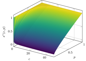
Figure 1: The surface of the optimal slope $s^{*}(c,p)$.

Another asymptotic scenario where $p\to 0$ but $c\to+\infty$ is investigated in the following result:

Lemma 6

Let $a\geq 1$, $b>0$, and $0<p<1/a$. Then

$$-a\gamma_{0}p\leq\underline{\Gamma}(b/p,p,ap)-\Gamma_{0}(a,b)\leq\gamma_{1}p\log\frac{1}{p}+e^{2}\gamma_{0}p,$$

where

$$\Gamma_{0}(a,b):=\int_{0}^{+\infty}e^{-x}r(abe^{-ax})\mathrm{d}x,$$

$\gamma_{0}=r(ab)$, and $\gamma_{1}=\gamma_{0}/2+a/4$.

Next, we evaluate the performance gap for the linear policy of slope $s^{*}(c,p)$ with respect to the throughput upper bound

$$\overline{\Gamma}(c,p):=r(pc)\quad\text{(\cite[cite]{[\@@bibref{}{ozgur2016universally}{}{}, Prop.~{}2]})}.$$ (12)

We consider the nominal multiplicative factor

$$F^{*}(c,p):=\frac{\underline{\Gamma}(c,p,s^{*}(c,p))}{\overline{\Gamma}(c,p)}$$

and the nominal additive gap

$$G^{*}(c,p):=\overline{\Gamma}(c,p)-\underline{\Gamma}(c,p,s^{*}(c,p)).$$

It is clear that for any $Q\in\mathcal{Q}_{c,p}$, $F^{*}(c,p)$ and $G^{*}(c,p)$ provide a lower bound on $F_{Q}(c,s^{*}(c,p))$ and an upper bound on $G_{Q}(c,s^{*}(c,p))$, respectively.

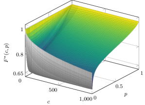
Figure 2: The surface of the nominal multiplicative factor $F^{*}(c,p)$.

A 3-D plot of $F^{*}(c,p)$ is shown in Fig. 2, which, together with Table II, indicates that the infimum of $F^{*}(c,p)$ occurs at $c\to\infty,p\to 0$ but $cp\to b$ for some $b>0$. The quantities $\underline{F}^{*}_{c}$ and $p^{*}(c)$ in Table II are defined by

$$\underline{F}^{*}_{c}:=\inf_{p\in(0,1)}F^{*}(c,p)$$

and

$$p^{*}(c):=\arg\inf_{p\in(0,1)}F^{*}(c,p).$$

It can be seen that the infimum of $F^{*}(c,p)$ is $\lim_{c\to+\infty}\underline{F}^{*}_{c}\approx 0.6530$ and meanwhile $\lim_{c\to+\infty}cp^{*}(c)\approx 1.7938$, both of which are consistent with the results of Proposition 9 to be introduced.

TABLE II: The Limits of $\underline{F}^{*}_{c}$ and $cp^{*}(c)$ as $c\to+\infty$

$c$	$p^{*}(c)$	$\underline{F}^{*}_{c}$	$cp^{*}(c)$
$10^{-3}$	0.000997	0.999501	9.970395e-07
$10^{-2}$	0.009708	0.995082	9.708167e-05
$10^{-1}$	0.076583	0.957074	7.658333e-03
$10^{0}$	0.211543	0.806004	2.115430e-01
$10^{1}$	0.105229	0.683399	1.052286e+00
$10^{2}$	0.016660	0.656616	1.665987e+00
$10^{3}$	0.001780	0.653408	1.779910e+00
$10^{4}$	0.000179	0.653079	1.792391e+00
$10^{5}$	0.000018	0.653046	1.793649e+00
$10^{6}$	0.000002	0.653043	1.793795e+00

Inspired by this observation, we proceed to determine the infimum of $F^{*}(c,p)$.

Fact 7

For $b>0$, $F^{*}(b/p,p)$ is non-decreasing in $p$.

Fact 8

$\alpha(b):=\lim_{p\to 0}s^{*}(b/p,p)/p<+\infty$ for all $b>0$.

Proposition 9

$$\underline{F}^{*} := \inf_{c>0,p\in(0,1)}F^{*}(c,p)$$

$$= \inf_{b>0}\max_{a\geq 1}\frac{\Gamma_{0}(a,b)}{r(b)}$$

$$= \frac{\Gamma_{0}(a^{*},b^{*})}{r(b^{*})}\approx 0.6530,$$

where the minimax occurs at the unique point $(a^{*},b^{*})$ defined by

$$a^{*}:=\hat{\alpha}(b^{*})=\alpha(b^{*})\approx 2.2847,$$ (13)

$$b^{*}:=\arg\inf_{b>0}\frac{\Gamma_{0}(\hat{\alpha}(b),b)}{r(b)}\approx 1.7938,$$ (14)

with

$$\hat{\alpha}(b):=\arg\max_{a\geq 1}\Gamma_{0}(a,b).$$ (15)

The infimum $\underline{F}^{*}\approx 0.6530$ indicates a $30\%$ improvement over the fixed fraction policy, whose actual multiplicative factor in the worst case is only $\frac{1}{2}$ [20, Th. 7]. In contrast, as the next proposition shows, the supremum of $G^{*}(c,p)$ is the same as the maximum nominal additive gap of fixed fraction policy.

Proposition 10

$\overline{G}^{*}:=\sup_{c>0,p\in(0,1)}G^{*}(c,p)=\frac{1}{2}$.

This is a straightforward consequence of the observation that the performance of the maximin optimal linear policy is bounded above and below by the maximin optimal policy and the fixed fraction policy, respectively, both of which have the same maximum nominal additive gap $\frac{1}{2}$ (nat) [16, Prop. 3] and [19, Table I].

III-B Worst-Case Optimal Linear Policy for Fixed MCR

In this subsection, we will go further to find universally good slope $s$ independent of battery capacity $c$. To formulate this problem, we consider the best worst-case performance compared to the upper bound (12). Specifically, we have two kinds of universally good linear policies in terms of multiplicative factor or additive gap:

1) $c$-universal optimal nominal multiplicative factor:

$$F^{\times}_{p}:=\max_{s\in(0,1]}\inf_{c>0}\frac{\underline{\Gamma}(c,p,s)}{\overline{\Gamma}(c,p)}$$

with the associated $c$-universal multiplicative-factor optimal linear policy of slope

$$s^{\times}(p):=\arg\max_{s\in(0,1]}\inf_{c>0}\frac{\underline{\Gamma}(c,p,s)}{\overline{\Gamma}(c,p)}.$$ (16)

2) $c$-universal optimal nominal additive gap:

$$G^{+}_{p}:=\min_{s\in(0,1]}\sup_{c>0}(\overline{\Gamma}(c,p)-\underline{\Gamma}(c,p,s))$$

with the associated $c$-universal additive-gap optimal linear policy of slope

$$s^{+}(p):=\arg\min_{s\in(0,1]}\sup_{c>0}(\overline{\Gamma}(c,p)-\underline{\Gamma}(c,p,s)).$$ (17)

First, we study the performance of $c$-universal multiplicative-factor optimal linear policy in the worst case (of $p$) as well as the approximation of $s^{\times}(p)$.

Fact 11

Let $p\in(0,1)$ and

$$F_{p}(c,s):=\frac{\underline{\Gamma}(c,p,s)}{\overline{\Gamma}(c,p)}.$$

Then

$$\max_{s\in(0,1]}\inf_{c>0}F_{p}(c,s)=\inf_{c>0}\max_{s\in(0,1]}F_{p}(c,s),$$

which occurs at the unique saddle point $(c^{\times}(p),s^{\times}(p))$, where $c^{\times}(p):=\arg\inf_{c>0}F_{p}(c,s^{\times}(p))$.

Proposition 12

$s^{\times}(p)=s^{*}(c^{\times}(p),p)$ for all $p\in(0,1)$.

Proposition 13

$\underline{F}^{\times}:=\inf_{p\in(0,1)}F^{\times}_{p}=\underline{F}^{*}$.

Since $\underline{F}^{\times}$, like $\underline{F}^{*}$, occurs at $p\to 0$, it is natural to conjecture that $\lim_{p\to 0}s^{\times}(p)/p=a^{*}$ and $\lim_{p\to 0}pc^{\times}(p)=b^{*}$.

Fact 14

As $p\to 0$, the limits of $pc^{\times}(p)$ and $s^{\times}(p)/p$ exist.

Proposition 15

$$a^{\times} := \lim_{p\to 0}\frac{s^{\times}(p)}{p}=a^{*},$$ (18)

$$b^{\times} := \lim_{p\to 0}pc^{\times}(p)=b^{*}.$$ (19)

where $a^{*}$ and $b^{*}$ are defined by (13) and (14), respectively.

Moreover, an accurate approximation of $s^{\times}(p)$ is obtained.

Fact 16

Let

$$\hat{s}^{\times}(p):=\min\left\{\frac{p}{2}\log(1+\tilde{s}(p))+\left(1-\frac{p}{2}\right)\tilde{s}(p),1\right\},$$

where

$$\tilde{s}(p):=(a^{*})^{0.05}\log(1+(a^{*})^{0.95}p).$$

Then $|\hat{s}^{\times}(p)-s^{\times}(p)|<0.0015$ for $p\in(0,1)$.

Both $s^{\times}(p)$ and $\hat{s}^{\times}(p)$ are plotted in Fig. 3.

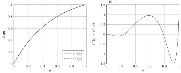
Figure 3: Plots of $s^{\times}(p)$, $\hat{s}^{\times}(p)$, and $\hat{s}^{\times}(p)-s^{\times}(p)$.

Next, we investigate the analytic expression and the worst-case performance of $c$-universal additive-gap optimal linear policy. As is shown by the next proposition, the $c$-universal additive-gap optimal linear policy turns out to be the fixed fraction policy.

Proposition 17

Let $p\in(0,1)$ and

$$G_{p}(c,s):=\overline{\Gamma}(c,p)-\underline{\Gamma}(c,p,s).$$

Then $G_{p}(c,s)$ is non-decreasing in $c$ for fixed $s$. Moreover, $s^{+}(p)=p$ and $\overline{G}^{+}:=\sup_{p\in(0,1)}G_{p}^{+}=\frac{1}{2}$.

In addition, it is worth evaluating the performance of $c$-universal multiplicative-factor optimal linear policy and $c$-universal additive-gap optimal linear policy in terms of additive gap and multiplicative factor, respectively. Therefore, we consider

$$\overline{G}^{\times}:=\sup_{c>0,p\in(0,1)}G_{p}(c,s^{\times}(p))$$

and

$$\underline{F}^{+}:=\sup_{c>0,p\in(0,1)}F_{p}(c,s^{+}(p)).$$

By [16, Prop. 4] and [20, Th. 7], it is clear that $\underline{F}^{+}=\frac{1}{2}$. As for $\overline{G}^{\times}$, we have the following result.

Proposition 18

$\overline{G}^{\times}=(a^{*}-\log a^{*})/2\approx 0.7292$.

IV Greedy Policy

In this section, we investigate a special linear policy—greedy policy. In [21], the greedy policy is shown to maximize the long-term average throughput in the small battery capacity regime. Specifically, it is proved that, given the reward function $r(x)$, the greedy policy is optimal if and only if

$$c\leq c^{*}(Q):=\max\left\{c\geq 0:r^{\prime}(c)\geq\int_{[0,c)}r^{\prime}(x)\mathrm{d}Q\right\},$$ (20)

where $Q$ is the marginal probability distribution of the i.i.d. process of energy arrivals. For the reward function (1), the threshold is given by

$$c^{*}(Q)=\max\left\{c\geq 0:\frac{1}{1+c}\geq\int_{[0,c)}\frac{1}{1+x}dQ\right\}.$$ (21)

As an example, we have $c^{*}=p/(1-p)$ for $Q=\tilde{\mathrm{B}}_{c,p}$ (see Proposition 1).

However, as the exact distribution of the energy arrival process is not always in hand, our aim in the sequel is to find the tightest bounds on the value of $c^{*}$ for certain families of energy arrival distributions. Specifically, we are interested in three cases, from general to special:

1) distribution $Q$ with the possible-value interval $[\underline{x},\overline{x}]$ (satisfying $Q([\underline{x},\overline{x}])=1$) and the mean $\mu$ ($\underline{x}\leq\mu\leq\overline{x}$);

2) clipped distribution $Q$ with the possible-value interval $[\underline{x},c]$ and the clipped mean $\bar{\mu}$ ($\underline{x}\leq\bar{\mu}\leq c$);

3) clipped distribution $Q$ with the possible-value interval $[0,c]$ and the MCR $p\in(0,1)$.

The proofs of results in this section are presented in Appendix C.

IV-A Semi-Universal Bounds on $c^{*}$ Given the Possible-Value Interval and Mean of an Energy Arrival Distribution

In this subsection, we will determine the tightest lower and upper bounds on $c^{*}$ given $\underline{x}$, $\overline{x}$, and $\mu$ of energy arrival distribution $Q$.

Definition 19

Let

$$\underline{c}(\underline{x},\overline{x},\mu):=\inf_{Q\in Q^{\prime}_{\underline{x},\overline{x},\mu}}c^{*}(Q)$$

and

$$\overline{c}(\underline{x},\overline{x},\mu):=\sup_{Q\in Q^{\prime}_{\underline{x},\overline{x},\mu}}c^{*}(Q),$$

where

$$\mathcal{Q}^{\prime}_{\underline{x},\overline{x},\mu}:=\{Q:Q([\underline{x},\overline{x}])=1,\mathbb{E}_{X\sim Q}X=\mu\}.$$

In order to find $\underline{c}(\underline{x},\overline{x},\mu)$ and $\overline{c}(\underline{x},\overline{x},\mu)$, one must maximize (minimize) the integral in (20). Thus, we need to find the values of

$$\overline{f}(c,\underline{x},\overline{x},\mu):=\sup_{Q\in\mathcal{Q}^{\prime}_{\underline{x},\overline{x},\mu}}\int_{[0,c)}r^{\prime}(x)\mathrm{d}Q$$

and

$$\underline{f}(c,\underline{x},\overline{x},\mu):=\inf_{Q\in\mathcal{Q}^{\prime}_{\underline{x},\overline{x},\mu}}\int_{[0,c)}r^{\prime}(x)\mathrm{d}Q,$$

The relation between $\underline{c}(\underline{x},\overline{x},\mu)$ (resp., $\overline{c}(\underline{x},\overline{x},\mu)$) and $\overline{f}(c,\underline{x},\overline{x},\mu)$ (resp., $\underline{f}(c,\underline{x},\overline{x},\mu)$) is established by the next lemma.

Lemma 20

Let $r$ be a non-decreasing, continuously differentiable, and strictly concave function on $[0,+\infty)$. Then,

$$\underline{c}(\underline{x},\overline{x},\mu)=\underline{c}^{\prime}(\underline{x},\overline{x},\mu):=\sup\left\{c\geq 0:r^{\prime}(c)\geq\overline{f}(c,\underline{x},\overline{x},\mu)\right\}$$

and

$$\overline{c}(\underline{x},\overline{x},\mu)=\overline{c}^{\prime}(\underline{x},\overline{x},\mu):=\sup\left\{c\geq 0:r^{\prime}(c)\geq\underline{f}(c,\underline{x},\overline{x},\mu)\right\}.$$

In the rest of this section, we will focus on the case of reward function (1). In this case, the exact values of $\underline{f}(c,\underline{x},\overline{x},\mu)$ and $\overline{f}(c,\underline{x},\overline{x},\mu)$ are determined by the next lemma.

Lemma 21

$$2\underline{f}(c,\underline{x},\overline{x},\mu)=\begin{cases}0&$c\in[0,\mu]$,\\ \frac{c-\mu}{(1+\underline{x})(c-\underline{x})}&$c\in[0, \iota(\text@underline{x})) \cap(\mu,\overline{x}]$,\\ \frac{4(c-\mu)}{(c+1)^{2}}&$c\in[\iota(\text@underline{x}),\iota(\mu)) \cap(\mu,\overline{x}]$,\\ \frac{1}{1+\mu}&$c\in[\iota(\mu),\overline{x}]\cup(\overline{x},+\infty)$,\end{cases}$$ (22)

$$2\overline{f}(c,\underline{x},\overline{x},\mu)=\begin{cases}0&$c\in[0,\text@underline{x}]$,\\ \frac{\overline{x}-\mu}{(\overline{x}-\underline{x})(1+\underline{x})}&$c\in[0,\tau]\cap(\text@underline{x},\overline{x}]$,\\ \frac{\overline{x}-\mu}{(\overline{x}-c)(1+c)}&$c\in(\tau,+\infty)\cap(\text@underline{x},\mu]$,\\ \frac{1+\underline{x}+c-\mu}{(1+\underline{x})(1+c)}&$c\in(\tau,+\infty)\cap(\mu,\overline{x}]$,\\ \frac{1+\underline{x}+\overline{x}-\mu}{(1+\underline{x})(1+\overline{x})}&$c\in(\overline{x},+\infty)$,\\ \end{cases}$$ (23)

where $\iota(x):=2x+1$ and $\tau:=\overline{x}-\underline{x}-1$.

Based on Lemma 21, we obtain $\underline{c}(\underline{x},\overline{x},\mu)$ and $\overline{c}(\underline{x},\overline{x},\mu)$.

Theorem 22

$$\underline{c}(\underline{x},\overline{x},\mu)=\begin{cases}\underline{c}_{1}&$\mu<\tau$,\\ \mu&$\mu\geq\tau$,\end{cases}$$

where

$$\underline{c}_{1}:=\frac{(\overline{x}-\underline{x})(1+\underline{x})}{\overline{x}-\mu}-1.$$

Corollary 23

$\underline{c}(\underline{x},\overline{x},\mu)=\overline{x}$ if and only if $\mu=\overline{x}$.

Theorem 24

$$\overline{c}(\underline{x},\overline{x},\mu)=\begin{cases}\min\{\overline{c}_{1},\overline{x}\}&$\mu<\frac{3}{2}\text@underline{x}+\frac{1}{2}$,\\ \min\{\overline{c}_{2},\overline{x}\}&$\mu\geq\frac{3}{2}\text@underline{x}+\frac{1}{2}$,\end{cases}$$

where

$$\overline{c}_{1}:=\frac{\underline{x}+\mu+\sqrt{(\underline{x}+\mu)^{2}-4(\underline{x}^{2}+\underline{x}-\mu)}}{2},$$

$$\overline{c}_{2}:=\frac{4\mu+1}{3}.$$

Corollary 25

$\overline{c}(\underline{x},\overline{x},\mu)=\overline{x}$ if and only if

$$\overline{x}\leq\begin{cases}\overline{c}_{1}&$\mu<\frac{3}{2}\text@underline{x}+\frac{1}{2}$,\\ \overline{c}_{2}&$\mu\geq\frac{3}{2}\text@underline{x}+\frac{1}{2}$.\end{cases}$$

Remark 26

The bounds given by Theorems 22 and 24 coincide with the bounds in [21, Props. 4 and 5], and hence the tightness of the former implies the tightness of the latter. This observation can be easily understood by the following trick. Let $Q$ be a distribution attaining $\underline{c}(\underline{x},\overline{x},\mu)$ or $\overline{c}(\underline{x},\overline{x},\mu)$. By definition, we only have $Q([\underline{x},\overline{x}])=1$, and in general, the essential infimum and supremum of a random variable with distribution $Q$ may be strictly larger than $\underline{x}$ and strictly less than $\overline{x}$, respectively. Consider a random variable $X_{t}$ with distribution

$$Q_{t}:=(1-t)Q+t\left(\frac{\overline{x}-\mu}{\overline{x}-\underline{x}}\delta_{\underline{x}}+\frac{\mu-\underline{x}}{\overline{x}-\underline{x}}\delta_{\overline{x}}\right)$$

where $t\in(0,1]$. Then, the essential minimum and maximum of $X_{t}$ are $\underline{x}$ and $\overline{x}$, respectively. Taking $t=1/n$, we obtain a sequence $\{Q_{1/n}\}_{n=1}^{\infty}$ of distributions approaching the bounds in [21, Props. 4 and 5].

IV-B Semi-Universal Bounds on $c^{*}$ Given the Least Possible Value and Mean of a Clipped Energy Arrival Distribution

In this subsection, we will determine the tightest lower and upper bounds on $c^{*}$ given $\underline{x}$, $\bar{\mu}$ of clipped energy arrival distribution $Q$.

Definition 27

Let

$$\underline{c}^{\prime}(\underline{x},\bar{\mu}):=\inf\{c\geq\bar{\mu}:c^{*}(Q)\geq c\ \text{for all $Q\in\mathcal{Q}^{\prime}_{\underline{x},c,\bar{\mu}}$}\}$$

and

$$\overline{c}^{\prime}(\underline{x},\bar{\mu}):=\sup\{c\geq\bar{\mu}:c^{*}(Q)\geq c\ \text{for some $Q\in\mathcal{Q}^{\prime}_{\underline{x},c,\bar{\mu}}$}\}.$$

By Corollaries 23 and 25 as well as the proof of Lemma 21, it is easy to determine the values of $\underline{c}^{\prime}(\underline{x},\bar{\mu})$ and $\overline{c}^{\prime}(\underline{x},\bar{\mu})$.

Theorem 28

$$\underline{c}^{\prime}(\underline{x},\bar{\mu}) = \bar{\mu},$$

$$\overline{c}^{\prime}(\underline{x},\bar{\mu}) = \begin{cases}\overline{c}_{1}&$\bar{\mu}<\frac{3}{2}\text@underline{x}+\frac{1}{2}$,\\ \overline{c}_{2}&$\bar{\mu}\geq\frac{3}{2}\text@underline{x}+\frac{1}{2}$,\end{cases}$$

where $\overline{c}^{\prime}(\underline{x},\bar{\mu})$ is attained by

$$\overline{Q}_{1}:=\begin{cases}\frac{c-\bar{\mu}}{c-\underline{x}}\delta_{\underline{x}}+\frac{\bar{u}-\underline{x}}{c-\underline{x}}\delta_{c}&$\bar{\mu}<\frac{3}{2}\text@underline{x}+\frac{1}{2}$,\\ \frac{2(c-\bar{\mu})}{c+1}\delta_{(c-1)/2}+\frac{2\bar{\mu}-c+1}{c+1}\delta_{c}&$\bar{\mu}\geq\frac{3}{2}\text@underline{x}+\frac{1}{2}$.\end{cases}$$

IV-C Semi-Universal Upper Bound on $c^{*}$ Given the MCR

In this subsection, we will determine the tightest upper bound on $c^{*}$ given MCR $p$ of clipped energy arrival distribution $Q$.

Definition 29

Let

$$\overline{c}^{\prime\prime}(p):=\sup\{c>0:c\leq\overline{c}^{\prime}(0,pc)\}.$$

Theorem 30

$$\overline{c}^{\prime\prime}(p)=\begin{cases}\frac{p}{1-p}&$p\in(0,\frac{1}{2})$,\\ \frac{1}{3-4p}&$p\in[\frac{1}{2},\frac{3}{4})$,\\ +\infty&$p\in[\frac{3}{4},1)$.\end{cases}$$

It can be attained by

$$\overline{Q}_{2}:=\begin{cases}(1-p)\delta_{0}+p\delta_{p/(1-p)}&$p\in(0,\frac{1}{2})$,\\ \frac{1}{2}\delta_{(2p-1)/(3-4p)}+\frac{1}{2}\delta_{1/(3-4p)}&$p\in[\frac{1}{2},\frac{3}{4})$,\end{cases}$$

and $\{\overline{Q}_{3}^{(n)}\}_{n=1}^{\infty}$ (for the last case) with

$$\overline{Q}_{3}^{(n)}:=\frac{2n(1-p)}{n+1}\delta_{(n-1)/2}+\frac{2pn-n+1}{n+1}\delta_{n}.$$

V Conclusion

We have systematically investigated linear power control policies for energy harvesting communications. Our formulations require a minimal amount of information regarding the energy arrival process, and consequently can capture various universality aspects of linear policies. The analysis of such formulations is feasible largely due to certain extremal properties of the Bernoulli energy arrival process and its variants. As shown in [20], to some extent, these extremal properties continue to be preserved even when a broader class of policies (not necessarily linear) are adopted. So it might be possible to expand the scope of our work by going beyond linear policies, which will enable a meaningful discussion of complexity vs. performance in the context of online power control.

Appendix A Numerical Verification of Facts in Sec. III

In order to provide a strong proof of the facts, we take the following methods in the numerical verification.

1) The verification process usually involves the computation of a one-variable function

$$f_{\xi_{1},\ldots,\xi_{k}}(x).$$

with parameters $\xi_{1}$, …, $\xi_{k}$. When $c$ or $p$ are the parameters of $f$, we choose by default

$$A:=\{j\times 10^{i}:-3\leq i\leq 2,1\leq j\leq 9\}\cup\{10^{3}\}$$

and

$$B:=\{10^{-3}\}\cup\{0.01i:1\leq i\leq 99\}$$

for the enumeration of $c$ and $p$, respectively. We also choose the values of

$$A_{1}:=\{10^{i}:i\geq-3\}$$

and

$$B_{1}:=\{0.001,0.01,0.1,0.5,0.9,0.99\}$$

as typical values of $c$ and $p$, respectively, for demonstration purposes.

2) In order to verify a qualitative property of a function $f(x)$, we take an adaptive sampling strategy to ensure that every pair of adjacent points, $(x,f(x))$ and $(x^{\prime},f(x^{\prime}))$, satisfies

$$|x-x^{\prime}|\leq d_{1}$$

or

$$\sqrt{(x-x^{\prime})^{2}+(f(x)-f(x^{\prime}))^{2}}\leq d_{2}.$$

The values of $d_{1}$ and $d_{2}$ are set to be $10^{-4}$ and $10^{-3}$, respectively.

3) In some cases, the domain of a function is not bounded. For example, the range of $c$ is $[0,+\infty)$. In this case, we consider a monotone transform, e.g.,

$$g(c^{\prime}):=\frac{c^{\prime}}{1-c^{\prime}}.$$

Then the domain of the new function $\hat{f}(c^{\prime}):=f(g(c^{\prime}))$ is $[0,1)$.

Proof:

It is verified that, for $(c,p)\in A\times B$ with $c>p/(1-p)$, $\underline{\Gamma}(c,p,s)$ is a unimodal function of $s$. As is shown by Table III, the slope $s^{*}_{2}$ obtained by solving (8) coincides with the optimal slope $s^{*}$ computed directly by a general optimization algorithm, except a minor difference in the first two rows, which is because $c$ and $p$ are so small that the default tolerance parameters of the algorithms are not small enough to ensure a completely consistent result.

TABLE III: Optimal Slopes $s^{*}$ (by General Optimization Algorithms) and $s^{*}_{2}$ (by Solving (8))

$c$	$p$	$s^{*}$	$\underline{\Gamma}(c,p,s^{*})$	$s^{*}_{2}$	$\underline{\Gamma}(c,p,s^{*}_{2})$
0.01	0.001	0.481011	0.000005	0.480988	0.000005
0.10	0.001	0.182497	0.000050	0.182496	0.000050
	0.010	0.485549	0.000487	0.485549	0.000487
1.00	0.001	0.062051	0.000485	0.062051	0.000485
	0.010	0.188597	0.004560	0.188597	0.004560
	0.100	0.531404	0.039166	0.531404	0.039166
10.00	0.001	0.020568	0.004540	0.020568	0.004540
	0.010	0.068740	0.037627	0.068740	0.037627
	0.100	0.251019	0.236875	0.251019	0.236875
	0.500	0.677521	0.698589	0.677521	0.698589
	0.900	0.992232	1.079208	0.992232	1.079208
100.00	0.001	0.007076	0.037480	0.007076	0.037480
	0.010	0.027547	0.229471	0.027547	0.229471
	0.100	0.141503	0.855315	0.141503	0.855315
	0.500	0.545454	1.650356	0.545454	1.650356
	0.900	0.918506	2.137336	0.918506	2.137336
	0.990	0.999903	2.284485	0.999903	2.284485
1000.00	0.001	0.002781	0.228762	0.002781	0.228762
	0.010	0.014573	0.838041	0.014573	0.838041
	0.100	0.109353	1.857101	0.109353	1.857101
	0.500	0.509370	2.766345	0.509370	2.766345
	0.900	0.903606	3.275259	0.903606	3.275259
	0.990	0.991160	3.426725	0.991160	3.426725

∎

Proof:

It is verified that $s^{*}(c,p)$ is non-decreasing in $p$ for $c\in A$ and is non-increasing in $c$ for $p\in B$. ∎

Proof:

It is verified that for fixed $b\in\{0.1i:i=1,2,\ldots,100\}\cup\{0.01,b^{*}\approx 1.7938,100\}$, $F^{*}(b/p,p)$ is non-decreasing on $[10^{-5},1]$, where $b^{*}$ is defined by (14). ∎

Proof:

As is shown by Table IV, the limit of $\lim_{p\to 0}s^{*}(b/p,p)/p$ exists and coincides with (15) for $b>0$.

TABLE IV: The Limit of $s^{*}(b/p,p)/p$ as $p\to 0$

$b$	$p=0.1$	$0.01$	$0.001$	$0.0001$	$0.00001$	$\hat{\alpha}(b)$
0.0010	10.000000	48.554922	62.051334	63.819945	64.002236	64.022630
0.0100	10.000000	18.859726	20.567566	20.754940	20.773864	20.775953
0.1000	5.314041	6.873961	7.076355	7.097194	7.099293	7.099519
0.5000	3.127759	3.553981	3.601971	3.606830	3.607317	3.607371
1.0000	2.510194	2.754738	2.781294	2.783972	2.784244	2.784270
1.5000	2.223322	2.400866	2.419834	2.421743	2.421931	2.421956
1.7938	2.112148	2.266523	2.282913	2.284562	2.284726	2.284745
2.0000	2.048791	2.190643	2.205649	2.207157	2.207309	2.207327
2.5000	1.928407	2.047797	2.060342	2.061603	2.061731	2.061743
3.0000	1.839015	1.942837	1.953693	1.954784	1.954892	1.954905

∎

Proof:

It is verified that Fact 11 holds for $p\in A$. See Table V for some examples of the saddle points.

TABLE V: The Saddle Points of $F_{p}(c,s)$

$p$	$\displaystyle\max_{s\in(0,1]}\inf_{c>0}F_{p}(c,s)$	the maximin point	$\displaystyle\inf_{c>0}\max_{s\in(0,1]}F_{p}(c,s)$	the minimax point
0.001	0.653247	(1795.415923, 0.002282)	0.653247	(1795.415904, 0.002282)
0.010	0.655090	(181.016024, 0.022600)	0.655090	(181.016024, 0.022600)
0.100	0.674155	(19.712070, 0.205705)	0.674155	(19.712069, 0.205705)
0.500	0.776854	(6.509979, 0.720563)	0.776854	(6.509980, 0.720563)
0.900	0.935771	(15.180153, 0.967304)	0.935771	(15.180150, 0.967304)
0.990	0.992095	(125.323723, 0.997956)	0.992095	(125.323729, 0.997956)

∎

Proof:

As is shown by Table VI, the limits of $pc^{\times}(p)$ and $s^{\times}(p)/p$ exist and coincide with the values $b^{*}$ and $a^{*}$, respectively.

TABLE VI: The Limits of $pc^{\times}(p)$ and $s^{\times}(p)/p$ as $p\to 0$

$p$	$c^{\times}(p)$	$s^{\times}(p)$	$pc^{\times}(p)$	$s^{\times}(p)/p$
0.10000	19.712069	0.205705	1.971207	2.057054
0.01000	181.016024	0.022600	1.810160	2.260028
0.00100	1795.415923	0.002282	1.795416	2.282255
0.00010	17939.539246	0.000228	1.793954	2.284499
0.00001	179381.073316	0.000023	1.793811	2.284725

∎

Proof:

It is verified that $|\hat{s}^{\times}(p)-s^{\times}(p)|<0.0015$ for $p\in\{i\times 10^{-3}:i=1,2,\ldots,10^{3}\}$. ∎

Appendix B Proofs of Results in Sec. III

Proof:

For $c\to 0$, it is clear that $s^{*}(c,p)=1$ because $s^{*}(c,p)=1$ for $c\leq p/(1-p)$. For $c\to+\infty$, it follows from (8) and the dominated convergence theorem that

$$\lim_{c\to+\infty}\left(\frac{s^{*}}{p}-1\right) = \lim_{c\to+\infty}\mathbb{E}_{N}\left(\frac{s^{*}(N+1)-1}{1+cs^{*}(1-s^{*})^{N}}\right)$$

$$= \mathbb{E}_{N}\lim_{c\to+\infty}\frac{s^{*}(N+1)-1}{1+cs^{*}(1-s^{*})^{N}}=0,$$

or equivalently, $\lim_{c\to+\infty}s^{*}(c,p)=p$. ∎

Proof:

On the one hand,

$$\underline{\Gamma}(b/p,p,ap) = \sum_{i=0}^{\infty}p(1-p)^{i}r(ab(1-ap)^{i})$$

$$\buildrel\textrm{(a)}\over{\leq} \sum_{i=0}^{\infty}pe^{-pi}r(abe^{-api})$$

$$= \sum_{i=0}^{N-1}pe^{-pi}r(abe^{-api})+\sum_{i=N}^{\infty}pe^{-pi}r(abe^{-api})$$

$$\buildrel\textrm{(b)}\over{\leq} \sum_{i=0}^{N-1}\left(\int_{pi}^{p(i+1)}pe^{-x}r(abe^{-ax})\mathrm{d}x+\gamma_{1}p^{2}\right)+e^{2}\gamma_{0}p$$

$$\leq \int_{0}^{+\infty}e^{-x}r(abe^{-ax})\mathrm{d}x+\gamma_{1}p\log\frac{1}{p}+e^{2}\gamma_{0}p,$$

where (a) follows from $1+x\leq e^{x}$ for $x\in\mathbb{R}$,

$$-\frac{\log p}{p}-1<N:=\left\lfloor-\frac{\log p}{p}\right\rfloor\leq-\frac{\log p}{p},$$

and (b) from Lemma 31 with

$$\sup_{x>0}|(e^{-x}r(abe^{-ax}))^{\prime}| = \sup_{x>0}(e^{-x}r(abe^{-ax})+a^{2}be^{-(1+a)x}r^{\prime}(abe^{-ax}))$$

$$\leq r(ab)+\sup_{x>0}\frac{a^{2}be^{-x}}{2(e^{ax}+ab)}$$

$$\leq r(ab)+\frac{a}{2}$$

and

$$\sum_{i=N}^{\infty}pe^{-pi}r(abe^{-api}) \leq pr(ab)e^{-pN}\sum_{i=0}^{\infty}e^{-pi}$$

$$= pr(ab)\frac{e^{-pN}}{1-e^{-p}}$$

$$\leq pr(ab)\frac{pe^{p}}{1-e^{-p}}$$

$$= p^{2}r(ab)\frac{e^{2p}}{e^{p}-1}$$

$$\leq p^{2}r(ab)\frac{e^{2}}{p}=e^{2}\gamma_{0}p.$$

On the other hand,

$$\underline{\Gamma}(b/p,p,ap) \buildrel\textrm{(a)}\over{\geq} \sum_{i=0}^{\infty}pe^{-pi/(1-p)}r(abe^{-api/(1-ap)})$$

$$\buildrel\textrm{(b)}\over{\geq} (1-ap)\sum_{i=0}^{\infty}\int_{pi/(1-ap)}^{p(i+1)/(1-ap)}e^{-pi/(1-ap)}r(abe^{-api/(1-ap)})\mathrm{d}x$$

$$= (1-ap)\int_{0}^{+\infty}e^{-x}r(abe^{-ax})\mathrm{d}x$$

$$\geq \int_{0}^{+\infty}e^{-x}r(abe^{-ax})\mathrm{d}x-a\gamma_{0}p,$$

where (a) follows from $1+x\geq e^{x/(1+x)}$ for $x>-1$ and (b) from Lemma 31. ∎

Proof:

We first show that

$$\lim_{p\to 0}\underline{\Gamma}(b/p,p,s^{*}(b/p,p))=\max_{a\geq 1}\Gamma_{0}(a,b)$$

for fixed $b>0$. By (11) and Fact 8,

$$\lim_{p\to 0}\underline{\Gamma}(b/p,p,s^{*}(b/p,p)) = \lim_{p\to 0}\max_{a\in[1,p^{-1/2}]}\underline{\Gamma}(b/p,p,ap)$$

$$\buildrel\textrm{(a)}\over{=} \lim_{p\to 0}\left(\max_{a\in[1,p^{-1/2}]}\Gamma_{0}(a,b)+\operatorname{O}\left((b+1)p^{1/2}\log\frac{1}{p}\right)\right)$$

$$= \max_{a\geq 1}\Gamma_{0}(a,b),$$

where (a) follows from Lemma 6.

Next, it is clear that $\Gamma_{0}(a,b)$ is a continuous function of $a$ for fixed $b$. It can also be verified numerically that $\Gamma_{0}(a,b^{*})$ has the unique maximum at $\hat{\alpha}(b^{*})\approx 2.2847$. Then by Lemma 6 and Fact 8 again, we have

$$\Gamma_{0}(\hat{\alpha}(b^{*}),b^{*}) = \lim_{p\to 0}\underline{\Gamma}(b^{*}/p,p,s^{*}(b^{*}/p,p))$$

$$= \lim_{p\to 0}\Gamma_{0}(s^{*}(b^{*}/p,p)/p,b^{*})$$

$$= \Gamma_{0}(\alpha(b^{*}),b^{*}),$$

which implies $\alpha(b^{*})=\hat{\alpha}(b^{*})$.

Finally, by definition,

$$\underline{F}^{*} = \inf_{c>0,p\in(0,1)}F^{*}(c,p)$$

$$= \inf_{b>0}\inf_{p\in(0,1)}F^{*}(b/p,p)$$

$$\buildrel\textrm{(a)}\over{=} \inf_{b>0}\lim_{p\to 0}F^{*}(b/p,p)$$

$$= \inf_{b>0}\frac{\lim_{p\to 0}\underline{\Gamma}(b/p,p,s^{*}(b/p,p))}{r(b)}$$

$$= \inf_{b>0}\max_{a\geq 1}\frac{\Gamma_{0}(a,b)}{r(b)}$$

$$= \frac{\Gamma_{0}(a^{*},b^{*})}{r(b^{*})}\approx 0.6530,$$

where (a) follows from the non-decreasing property of $F^{*}(b/p,p)$ (Fact 7), and the last approximation is obtained at $b^{*}\approx 1.7938$ with $a^{*}=\hat{\alpha}(b^{*})\approx 2.2847$. It is also easy to verify numerically that the minimax point $(a^{*},b^{*})$ is unique. ∎

Proof:

Since $(c^{\times}(p),s^{\times}(p))$ is a saddle point of $F_{p}(c,s)$ (Fact 11), it follows that

$$s^{\times}(p) = \arg\max_{s\in(0,1]}F_{p}(c^{\times}(p),s)$$

$$= \arg\max_{s\in(0,1]}\underline{\Gamma}(c^{\times}(p),p,s)=s^{*}(c^{\times}(p),p).$$

∎

Proof:

$$\underline{F}^{\times} = \inf_{p\in(0,1)}\max_{s\in(0,1]}\inf_{c>0}\frac{\underline{\Gamma}(c,p,s)}{\overline{\Gamma}(c,p)}$$

$$\buildrel\textrm{(a)}\over{=} \inf_{p\in(0,1)}\inf_{c>0}\max_{s\in(0,1]}\frac{\underline{\Gamma}(c,p,s)}{\overline{\Gamma}(c,p)}$$

$$= \inf_{p\in(0,1)}\inf_{c>0}\frac{\underline{\Gamma}(c,p,s^{*}(c,p))}{\overline{\Gamma}(c,p)}$$

$$= \inf_{c>0,p\in(0,1)}F^{*}(c,p)=\underline{F}^{*},$$

where (a) follows from Fact 11. ∎

Proof:

By a similar argument to the proof of Proposition 13, we have $F_{p}(c^{\times}(p),s^{\times}(p))=\inf_{c>0}F^{*}(c,p)$. It is also easy to see that

$$\inf_{c>0}F^{*}(c,p)\geq\inf_{c>0}F^{*}\left(\frac{cp}{p^{\prime}},p^{\prime}\right)=\inf_{c>0}F^{*}(c,p^{\prime})$$

for $p^{\prime}<p$ (Fact 7). Then by Propositions 9 and 13,

$$\lim_{p\to 0}F_{p}(c^{\times}(p),s^{\times}(p))=\underline{F}^{\times}=\inf_{b\geq 1}\max_{a\geq 1}\frac{\Gamma_{0}(a,b)}{r(b)}=\frac{\Gamma_{0}(a^{*},b^{*})}{r(b^{*})}.$$

On the other hand, by Lemma 6 and a similar argument to the proof of Proposition 9,

$$\lim_{p\to 0}F_{p}(c^{\times}(p),s^{\times}(p)) = \lim_{p\to 0}\frac{\underline{\Gamma}(c^{\times}(p),p,s^{*}(c^{\times}(p),p))}{r(pc^{\times}(p))}$$

$$= \max_{a\geq 1}\frac{\Gamma_{0}(a,b^{\times})}{r(b^{\times})}.$$

The uniqueness of the minimax point $(a^{*},b^{*})$ then implies $b^{\times}=b^{*}$ and $a^{\times}=a^{*}$. ∎

Proof:

We first show that $G_{p}(c,s)$ is non-decreasing in $c$ for any fixed $s\in(0,1]$. For any $c>0$ and $s\in(0,1]$.

$$\frac{\partial G_{p}(c,s)}{\partial c} = pr^{\prime}(pc)-\sum_{i=0}^{\infty}p(1-p)^{i}r^{\prime}(cs(1-s)^{i})s(1-s)^{i}$$

$$= \frac{p}{2(1+pc)}-\frac{1}{2c}\sum_{i=0}^{\infty}p(1-p)^{i}\frac{cs(1-s)^{i}}{1+cs(1-s)^{i}}$$

$$\buildrel\textrm{(a)}\over{\geq} \frac{p}{2(1+pc)}-\frac{\hat{\mu}}{2c(1+\hat{\mu})}\geq 0,$$

where (a) follows from Jensen’s inequality with the concavity of $x/(1+x)$ (for $x>0$) and

$$\hat{\mu} := psc\sum_{i=0}^{\infty}[(1-p)(1-s)]^{i}$$

$$= \frac{psc}{1-(1-p)(1-s)}$$

$$= \frac{c}{1/p+1/s-1}\leq pc.$$

Then,

$$\min_{s\in(0,1]}\sup_{c>0}G_{p}(c,s) = \min_{s\in(0,1]}\lim_{c\to+\infty}G_{p}(c,s)$$

$$= \min_{s\in(0,1]}\lim_{c\to+\infty}\frac{1}{2}\sum_{i=0}^{\infty}p(1-p)^{i}\log\left[\frac{1+cp}{1+cs(1-s)^{i}}\right]$$

$$= \min_{s\in(0,1]}\frac{1}{2}\sum_{i=0}^{\infty}p(1-p)^{i}\left[\log\frac{p}{s}-i\log(1-s)\right]$$

$$= \min_{s\in(0,1]}G_{p}(s)=G_{p}(p),$$

where

$$G_{p}(s):=\frac{1}{2}\left(\log\frac{p}{s}-\frac{1-p}{p}\log(1-s)\right)$$ (24)

with its minimum occurring at $s=p$. Therefore, $s^{+}(p)=p$ and hence $\overline{G}^{+}=\inf_{p\in(0,1)}G_{p}(p)=\lim_{p\to 0}G_{p}(p)=\frac{1}{2}$ (see also [16, Prop. 3]). ∎

Proof:

By Proposition 17 and a similar argument to its proof, we have

$$\overline{G}^{\times} = \sup_{p\in(0,1)}\lim_{c\to+\infty}G_{p}(c,s^{\times}(p))$$

$$= \sup_{p\in(0,1)}G_{p}(s^{\times}(p))$$

$$\buildrel\textrm{(a)}\over{=} \lim_{p\to 0}G_{p}(s^{\times}(p))$$

$$\buildrel\textrm{(b)}\over{=} \frac{a^{*}-\log a^{*}}{2}\approx 0.7292,$$

where $G_{p}(s)$ is defined by (24), (a) is verified numerically (Fig. 4), and (b) follows from (18).

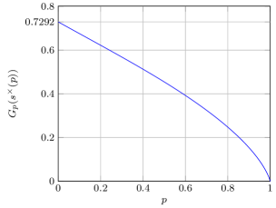
Figure 4: Plot of $G_{p}(s^{\times}(p))$ versus $p$.

∎

Appendix C Proofs of Results in Sec. IV

Proof:

By definition, for any $c<\underline{c}^{\prime}(\underline{x},\overline{x},\mu)$,

$$r^{\prime}(c)\geq\overline{f}(c,\underline{x},\overline{x},\mu)\geq\int_{[0,c)}r^{\prime}(x)\mathrm{d}Q$$

for all $Q\in Q^{\prime}_{\underline{x},\overline{x},\mu}$, which implies $c\leq c^{*}(Q)$ for all $Q\in Q^{\prime}_{\underline{x},\overline{x},\mu}$, hence $c\leq\underline{c}(\underline{x},\overline{x},\mu)$, and therefore $\underline{c}^{\prime}(\underline{x},\overline{x},\mu)\leq\underline{c}(\underline{x},\overline{x},\mu)$. On the other hand, for any $c<\underline{c}(\underline{x},\overline{x},\mu)$,

$$r^{\prime}(c)\geq\int_{[0,c)}r^{\prime}(x)\mathrm{d}Q$$

for all $Q\in Q^{\prime}_{\underline{x},\overline{x},\mu}$, that is, $r^{\prime}(c)\geq\overline{f}(c,\underline{x},\overline{x},\mu)$, which implies $c\leq\underline{c}^{\prime}(\underline{x},\overline{x},\mu)$, and hence $\underline{c}(\underline{x},\overline{x},\mu)\leq\underline{c}^{\prime}(\underline{x},\overline{x},\mu)$. Therefore, $\underline{c}(\underline{x},\overline{x},\mu)=\underline{c}(\underline{x},\overline{x},\mu)$.

Similarly, for any $c<\overline{c}^{\prime}(\underline{x},\overline{x},\mu)$,

$$r^{\prime}(c)>r^{\prime}\left(\frac{c+\overline{c}^{\prime}(\underline{x},\overline{x},\mu)}{2}\right)\\ \geq\underline{f}\left(\frac{c+\overline{c}^{\prime}(\underline{x},\overline{x},\mu)}{2},\underline{x},\overline{x},\mu\right)\geq\underline{f}(c,\underline{x},\overline{x},\mu),$$

and hence

$$r^{\prime}(c)\geq\int_{[0,c)}r^{\prime}(x)\mathrm{d}Q$$

for some $Q\in Q^{\prime}_{\underline{x},\overline{x},\mu}$. This implies $c\leq c^{*}(Q)\leq\overline{c}(\underline{x},\overline{x},\mu)$, and hence $\overline{c}^{\prime}(\underline{x},\overline{x},\mu)\leq\overline{c}(\underline{x},\overline{x},\mu)$. Moreover, for any $c<\overline{c}(\underline{x},\overline{x},\mu)$, there exists a $Q\in Q^{\prime}_{\underline{x},\overline{x},\mu}$ such that

$$r^{\prime}(c)\geq\int_{[0,c)}r^{\prime}(x)\mathrm{d}Q\geq\underline{f}(c,\underline{x},\overline{x},\mu).$$

This implies $c\leq\overline{c}^{\prime}(\underline{x},\overline{x},\mu)$, and hence $\overline{c}(\underline{x},\overline{x},\mu)\leq\overline{c}^{\prime}(\underline{x},\overline{x},\mu)$. ∎

Proof:

The problem to be solved is a linear program in a measure space. By [24, Th. 3.1], the optimal value, minimum or maximum, must occur at an extreme point of the set of feasible probability measures, all probability measures $Q$ satisfying the constraints

$$\int_{\mathbb{R}_{\geq 0}}\mathrm{d}Q=1\ \text{and}\ \int_{\mathbb{R}_{\geq 0}}x\mathrm{d}Q=\mu.$$

It follows from [24, Th. 3.2] that such an extreme point $Q$ must be a discrete probability measure concentrated at one or two points. Therefore, it suffices to consider $Q$ of the form $Q(\mu)=1$ or

$$Q(a)=\frac{b-\mu}{b-a}\ \text{and}\ Q(b)=\frac{\mu-a}{b-a}$$

with $\underline{x}\leq a<\mu<b\leq\overline{x}$. The optimization problem then reduces to the following simplified forms:

$$\underline{g}(c,\underline{x},\overline{x},\mu):=\begin{cases}0&$c \leq\mu$,\\ \displaystyle\min\left\{\underline{g}_{a,b}(c),\frac{1}{1+\mu}\right\}&$c > \mu$,\end{cases}$$

and

$$\overline{g}(c,\underline{x},\overline{x},\mu):=\begin{cases}\overline{g}_{a,b}(c)&$c \leq\mu$,\\[4.30554pt] \displaystyle\max\left\{\overline{g}_{a,b}(c),\frac{1}{1+\mu}\right\}&$c > \mu$,\end{cases}$$

where

$$\underline{g}_{a,b}(c):=\inf_{\underline{x}\leq a<\mu<b\leq\overline{x}}g_{a,b}(c),$$

$$\overline{g}_{a,b}(c):=\sup_{\underline{x}\leq a<\mu<b\leq\overline{x}}g_{a,b}(c),$$

and

$$g_{a,b}(c):=\frac{b-\mu}{(b-a)(1+a)}1\{c>a\}+\frac{\mu-a}{(b-a)(1+b)}1\{c>b\}.$$

1) If $c>b$, then

$$g_{a,b}(c)=\frac{b-\mu}{(b-a)(1+a)}+\frac{\mu-a}{(b-a)(1+b)}.$$

By the convexity of $1/(1+x)$ (for $x\geq 0$), the infimum and the supremum of $g_{a,b}(c)$ are attained as $(a,b)\to(\mu,\mu)$ (Jensen’s inequality) and $(a,b)\to(\underline{x},c^{\prime})$ ([16, Lemma 2]), respectively, where

$$c^{\prime}:=\min\{c,\overline{x}\},$$

so

$$\underline{g}_{a,b}(c)=\frac{1}{1+\mu}\ \text{and}\ \overline{g}_{a,b}(c)=\frac{1+\underline{x}+c^{\prime}-\mu}{(1+\underline{x})(1+c^{\prime})}.$$

2) If $\mu<c\leq b$, then

$$g_{a,b}(c)=\frac{b-\mu}{(b-a)(1+a)}=\frac{1}{1+a}-\frac{\mu-a}{(b-a)(1+a)},$$ (25)

which is strictly increasing in $b$ for any fixed $a$ and $c$. On the other hand,

$$g_{a,b}(c)=\frac{b-\mu}{-\left(a-\frac{b-1}{2}\right)^{2}+\frac{(b+1)^{2}}{4}},$$

which is strictly decreasing and strictly increasing in $a$ for $a<(b-1)/2$ and $a>(b-1)/2$, respectively. Thus, taking $b=c$ and according to the position of

$$a_{0}:=\frac{b-1}{2}=\frac{c-1}{2}$$

(compared to $\underline{x}$ and $\mu$), we have

$$\underline{g}_{a,b}(c) = \begin{cases}g_{\underline{x},c}(c)&$a_0<\text@underline{x}$,\\ g_{a_{0},c}(c)&$\text@underline{x}\leq a_0<\mu$,\\ g_{\mu,c}(c)&$a_0\geq\mu$,\end{cases}=\begin{cases}\frac{c-\mu}{(c-\underline{x})(1+\underline{x})}&$c\in[0,\iota(\text@underline{x}))\cap(\mu, \overline{x}]$,\\ \frac{4(c-\mu)}{(c+1)^{2}}&$c\in[\iota(\text@underline{x}),\iota(\mu))\cap(\mu, \overline{x}]$,\\ \frac{1}{1+\mu}&$c\in[\iota(\mu),+\infty)\cap(\mu, \overline{x}]$.\end{cases}$$

Similarly, taking $b=\overline{x}$ and comparing

$$a_{1}:=\frac{b-1}{2}=\frac{\overline{x}-1}{2}$$ (26)

with

$$a_{2}:=\frac{\underline{x}+\mu}{2},$$

we have

$$\overline{g}_{a,b}(c) = \begin{cases}g_{\mu,\overline{x}}(c)&$a_1<a_2$,\\ g_{\underline{x},\overline{x}}(c)&$a_1\geq a_2$,\end{cases}=\begin{cases}\frac{1}{1+\mu}&$\mu>\tau$,\\ \frac{\overline{x}-\mu}{(\overline{x}-\underline{x})(1+\underline{x})}&$\mu\leq\tau$.\end{cases}$$

3) If $a<c\leq\mu$, we also have (25). Thus, taking $b=\overline{x}$ and comparing $a_{1}$ (defined by (26)) with

$$a_{3}:=\frac{\underline{x}+c}{2},$$

we have

$$\overline{g}_{a,b}(c) = \begin{cases}g_{c,\overline{x}}(c)&$a_1<a_3$,\\ g_{\underline{x},\overline{x}}(c)&$a_1\geq a_3$,\end{cases}=\begin{cases}\frac{\overline{x}-\mu}{(\overline{x}-c)(1+c)}&$c>\tau$,\\ \frac{\overline{x}-\mu}{(\overline{x}-\underline{x})(1+\underline{x})}&$c\leq\tau$.\end{cases}$$

4) If $c\leq a$, then $g_{a,b}(c)=0$.

Combining Parts (1)–(4) gives (22) and (23). Some of the cases in (23) are slightly complicated, because the comparison of several candidates of the maximum are need as follows:

$$\frac{1}{1+\mu}<\frac{1+\underline{x}+c-\mu}{(1+\underline{x})(1+c)}\quad\text{for $c\in(\mu,\overline{x}]$}$$

and

$$\frac{\overline{x}-\mu}{(\overline{x}-\underline{x})(1+\underline{x})}\lesseqqgtr\frac{1+\underline{x}+c-\mu}{(1+\underline{x})(1+c)}\quad\text{for $c\gtreqqless\tau$ and $c\in(\mu,\overline{x}]$.}$$

∎

Proof:

It is clear that

$$\underline{c}_{1}\lesseqqgtr\tau\quad\text{for $\mu\lesseqqgtr\tau$}.$$

By Lemmas 20 and 21,

$$\underline{c}(\underline{x},\overline{x},\mu) = \sup([0,\underline{x}]\cup A\cup B)=\begin{cases}\underline{c}_{1}&$\mu<\tau$,\\ \mu&$\mu\geq\tau$,\end{cases}$$

where

$$A = [0,\underline{c}_{1}]\cap[0,\tau]\cap(\underline{x},\overline{x}]=\begin{cases}(\underline{x},\underline{c}_{1}]&$\mu<\tau$,\\ {}(\underline{x},\tau]&$\mu\geq\tau$,\end{cases}$$

$$B = (\tau,+\infty)\cap(\underline{x},\mu].$$

∎

Proof:

Note that

$$\overline{c}_{1}\lesseqqgtr\iota(\underline{x})\quad\text{for $\mu\lesseqqgtr\frac{3}{2}\underline{x}+\frac{1}{2}$}$$

and

$$\overline{c}_{2}\lesseqqgtr\iota(\underline{x})\quad\text{for $\mu\lesseqqgtr\frac{3}{2}\underline{x}+\frac{1}{2}$}.$$

By Lemmas 20 and 21,

$$\overline{c}(\underline{x},\overline{x},\mu) = \sup([0,\mu]\cup A\cup B)=\begin{cases}\min\{\overline{c}_{1},\overline{x}\}&$\mu<\frac{3}{2}\text@underline{x}+\frac{1}{2}$,\\ \min\{\overline{c}_{2},\overline{x}\}&$\mu\geq\frac{3}{2}\text@underline{x}+\frac{1}{2}$,\end{cases}$$

where

$$A = [0,\overline{c}_{1}]\cap[0,\iota(\underline{x})]\cap(\mu,\overline{x}],$$

$$B = [\iota(\underline{x}),\overline{c}_{2}]\cap(\mu,\overline{x}].$$

∎

Proof:

Let $f(x):=\overline{c}^{\prime}(0,x)$. By Theorem 28,

$$f(x)=\begin{cases}\frac{x+\sqrt{x^{2}+4x}}{2}&$x<\frac{1}{2}$,\\ \frac{4}{3}x+\frac{1}{3}&$x\geq\frac{1}{2}$.\end{cases}$$

Then for $x<\frac{1}{2}$,

$$f^{\prime}(x)=\frac{1}{2}+\frac{x+2}{2(x^{2}+4x)^{1/2}}>0$$

and

$$f^{\prime\prime}(x) = \frac{2(x^{2}+4x)^{1/2}-2(x+2)^{2}(x^{2}+4x)^{-1/2}}{4(x^{2}+4x)}$$

$$= \frac{2(x^{2}+4x)-2(x+2)^{2}}{4(x^{2}+4x)^{3/2}}=-\frac{2}{(x^{2}+4x)^{3/2}}<0.$$

It is clear that $f^{\prime}(0)=+\infty$ and $f$ is differentiable at $x=1/2$ with $f^{\prime}(\frac{1}{2})=\frac{4}{3}$. Hence $f$ is strictly increasing and concave on $[0,+\infty)$, and therefore, for every $p\in(0,1)$, $\overline{c}^{\prime\prime}(p)$ is the unique positive solution of $c=f(pc)$ (if exists) or $+\infty$. Solving the equation then gives

$$\overline{c}^{\prime\prime}(p)=\begin{cases}\frac{p}{1-p}&$p\in(0,\frac{1}{2})$,\\ \frac{1}{3-4p}&$p\in[\frac{1}{2},\frac{3}{4})$,\\ +\infty&$p\in[\frac{3}{4},1)$.\end{cases}$$

The verification of the remaining part of the theorem is straightforward. ∎

Appendix D Some Useful Results

Lemma 31

If $f:[a,b]\to\mathbb{R}$ is continuous on $[a,b]$, differentiable on $(a,b)$, and satisfies $f(x)\leq f(a)$ for all $x\in[a,b]$, then

$$f(a)(b-a)-\frac{1}{2}A(b-a)^{2}\leq\int_{a}^{b}f(x)\mathrm{d}x\leq f(a)(b-a),$$

where $A=\sup_{x\in(a,b)}|f^{\prime}(x)|$.

Proof:

Observe that

$$0\leq f(a)-f(x)\leq A(x-a)$$

by the mean value theorem, Taking integration over $[a,b]$, we obtain

$$0\leq\int_{a}^{b}(f(a)-f(x))\mathrm{d}x\leq\frac{1}{2}A(b-a)^{2},$$

which concludes the lemma. ∎

References

- [1] V. Sharma, U. Mukherji, V. Joseph, and S. Gupta, “Optimal energy management policies for energy harvesting sensor nodes,” IEEE Trans. Wireless Commun., vol. 9, no. 4, pp. 1326–1336, Apr. 2010.
- [2] O. Ozel, K. Tutuncuoglu, J. Yang, S. Ulukus, and A. Yener, “Transmission with energy harvesting nodes in fading wireless channels: Optimal policies,” IEEE J. Sel. Areas Commun., vol. 29, no. 8, pp. 1732–1743, Sep. 2011.
- [3] J. Yang and S. Ulukus, “Optimal packet scheduling in an energy harvesting communication system,” IEEE Trans. Commun., vol. 60, no. 1, pp. 220–230, Jan. 2012.
- [4] K. Tutuncuoglu and A. Yener, “Optimum transmission policies for battery limited energy harvesting nodes,” IEEE Trans. Wireless Commun., vol. 11, no. 3, pp. 1180–1189, Mar. 2012.
- [5] C. K. Ho and R. Zhang, “Optimal energy allocation for wireless communications with energy harvesting constraints,” IEEE Trans. Signal Process., vol. 60, no. 9, pp. 4808–4818, Sep. 2012.
- [6] O. Ozel and S. Ulukus, “Achieving AWGN capacity under stochastic energy harvesting,” IEEE Trans. Inf. Theory, vol. 58, no. 10, pp. 6471–6483, Oct. 2012.
- [7] P. Blasco, D. Gunduz, and M. Dohler, “A learning theoretic approach to energy harvesting communication system optimization,” IEEE Trans. Wireless Commun., vol. 12, no. 4, pp. 1872–1882, Apr. 2013.
- [8] Q. Wang and M. Liu, “When simplicity meets optimality: Efficient transmission power control with stochastic energy harvesting,” in Proc. IEEE INFOCOM 2013, Apr. 2013, pp. 580–584.
- [9] R. Srivastava and C. E. Koksal, “Basic performance limits and tradeoffs in energy-harvesting sensor nodes with finite data and energy storage,” IEEE/ACM Trans. Netw., vol. 21, no. 4, pp. 1049–1062, Aug. 2013.
- [10] M. B. Khuzani and P. Mitran, “On online energy harvesting in multiple access communication systems,” IEEE Trans. Inf. Theory, vol. 60, no. 3, pp. 1883–1898, Mar. 2014.
- [11] J. Xu and R. Zhang, “Throughput optimal policies for energy harvesting wireless transmitters with non-ideal circuit power,” IEEE J. Sel. Areas Commun., vol. 32, no. 2, pp. 322–332, Feb. 2014.
- [12] R. Rajesh, V. Sharma, and P. Viswanath, “Capacity of Gaussian channels with energy harvesting and processing cost,” IEEE Trans. Inf. Theory, vol. 60, no. 5, pp. 2563–2575, May 2014.
- [13] S. Ulukus, A. Yener, E. Erkip, O. Simeone, M. Zorzi, P. Grover, and K. Huang, “Energy harvesting wireless communications: A review of recent advances,” IEEE J. Sel. Areas Commun., vol. 33, no. 3, pp. 360–381, Mar. 2015.
- [14] Y. Dong, F. Farnia, and A. Özgür, “Near optimal energy control and approximate capacity of energy harvesting communication,” IEEE J. Sel. Areas Commun., vol. 33, no. 3, pp. 540–557, Mar. 2015.
- [15] F. Amirnavaei and M. Dong, “Online power control optimization for wireless transmission with energy harvesting and storage,” IEEE Trans. Wireless Commun., pp. 4888–4901, Jul. 2016.
- [16] D. Shaviv and A. Özgür, “Universally near optimal online power control for energy harvesting nodes,” IEEE J. Sel. Areas Commun., vol. 34, no. 12, pp. 3620–3631, Dec. 2016.
- [17] ——, “Approximately optimal policies for a class of Markov decision problems with applications to energy harvesting,” in Proc. 2017 15th International Symposium on Modeling and Optimization in Mobile, Ad Hoc, and Wireless Networks (WiOpt). Paris, France: IEEE, May 2017, pp. 1–8.
- [18] A. Arafa, A. Baknina, and S. Ulukus, “Online fixed fraction policies in energy harvesting communication systems,” IEEE Trans. Wireless Commun., vol. 17, no. 5, pp. 2975–2986, May 2018.
- [19] S. Yang and J. Chen, “A maximin optimal online power control policy for energy harvesting communications,” in Proc. 2020 IEEE International Conference on Communications (ICC). Dublin, Ireland: IEEE, Jun. 2020, pp. 1–6.
- [20] ——, “A maximin optimal online power control policy for energy harvesting communications,” IEEE Trans. Wireless Commun., vol. 19, no. 10, pp. 6708–6720, Oct. 2020.
- [21] Y. Wang, A. Zibaeenejad, Y. Jing, and J. Chen, “On the optimality of the greedy policy for battery limited energy harvesting communications,” IEEE Trans. Inf. Theory, vol. 67, no. 10, pp. 6548–6563, Oct. 2021.
- [22] A. Zibaeenejad, S. Yang, and J. Chen, “On optimal power control for energy harvesting communications with lookahead,” IEEE Trans. Wireless Commun., vol. 21, no. 6, pp. 4054–4067, Jun. 2022.
- [23] A. Arapostathis, V. S. Borkar, E. Fernández-Gaucherand, M. K. Ghosh, and S. I. Marcus, “Discrete-Time Controlled Markov Processes with Average Cost Criterion: A Survey,” SIAM J. Control Optim., vol. 31, no. 2, pp. 282–344, Mar. 1993.
- [24] H. Lai and S. Wu, “Linear programming in measure spaces,” Optimization, vol. 29, no. 2, pp. 141–156, Jan. 1994.