Globally stable and locally optimal model predictive control using a softened initial state constraint - extended version

Abstract

To address feasibility issues in model predictive control (MPC), most implementations relax hard state constraints using additional slack variables with a suitable penalty. We propose an alternative strategy for open-loop asymptotically/Lyapunov stable nonlinear systems by relaxing the initial state constraint with a suitable penalty. The proposed MPC framework is globally feasible, ensures (semi-)global asymptotic stability, and (approximately) recovers the closed-loop properties of the nominal MPC on the feasible set. The proposed framework can be naturally combined with a robust formulation to ensure robustness subject to bounded disturbances while retaining input-ot-state stability in case of arbitrarily large disturbances. We also show how the overall design can be simplified in case the nonlinear system is exponentially stable. In the special case of linear systems, the proposed MPC formulation reduces to a quadratic program and the offline design and online computational complexity is only marginally increased compared to anominal design. Benefits compared to classical soft contrained MPC formulations are demonstrated with numerical examples.

I Introduction

Model predictive control (MPC) is an optimization-based control technique that is applicable to general nonlinear systems and can incorporate both state and input constraints [1, 2]. The main desired properties of MPC schemes are (approximate/local) optimality, asymptotic stability, and closed-loop constraint satisfaction for a large set of initial conditions. However, these properties are typically based on the presence of hard constraints in the MPC optimization problem, which in turn can lead to a loss of feasibility during run-time, e.g., due to unexpected disturbances. Hence, to avoid feasibility issues, constraints are often relaxed and replaced by a suitable penalty on constraint violation, which is commonly referred to as soft constraints [3, 4, 5, 6, 7, 8, 9, 10, 11]. However, even if soft state constraints are considered, existing MPC formulations need to trade off global stability and local optimality in the offline design of the terminal ingredients. In this paper, we consider open-loop asymptotically/Lyapunov stable systems and provide a (semi-)globally asymptotically stable MPC formulation, which (approximately) recovers optimality and state constraint satisfaction on the feasible set by relaxing the initial state constraint.

Related work

For linear stable systems without state constraints, a globally stabilizing MPC can be designed using the infinite-horizon open-loop cost as a terminal penalty [12, Thm. 1]. To account for state constraints, [4] penalizes the peak constraint violation over the infinite-horizon, which preserves global stability. In [5], standard point-wise in time constraint violations are penalized, but the corresponding infinite-horizon terminal penalty increases the computational complexity. Using the fact that the penalty on constraint violation is quadratically bounded, a globally valid quadratic terminal penalty ensuring stability can be constructed [11]. In general, these MPC formulations ensure global stability, but the corresponding terminal penalties are rather conservative over-approximations of the infinite-horizon optimal cost, resulting in a deterioration of the closed-loop performance.

For stabilizable linear systems with quadratic stage cost and both state and input constraints, infinite-horizon optimal performance, i.e., the constrained linear quadratic regulator (LQR), can be achieved by defining the terminal ingredients based on the LQR and choosing a sufficiently large prediction horizon (in dependence of the initial condition), compare [13, 14, 15]. However, for a fixed prediction horizon, the presence of hard state and terminal constraints yields a bounded feasible set. This feasible set can be increased by relaxing the state constraints using soft constraints and even further by partially softening the terminal set constraint [8]. This MPC formulation is further extended to a softened polytopic terminal set in [9], compare also [10]. These MPC formulations can achieve local optimality, but the terminal set constraints cannot be completely relaxed and thus feasibility issues may still occur in closed loop.

For nonlinear systems subject to state and input constraints, assuming stabilizability of the linearization, suitable terminal ingredients can be computed based on the LQR [16], resulting in (locally) approximately optimal controllers (cf. [17, Thm. 6.4]) with a bounded feasible set. The corresponding terminal set constraint can also be omitted to provide a globally feasible MPC formulation, however, the corresponding closed-loop properties are only valid on some strict subset [18]. For a certain class of nonlinear stabilizable systems without state constraints, MPC formulations without terminal ingredients can ensure (semi-)global asymptotic stability with a sufficiently large prediction horizon, compare [19, 17], [2, Chap. 6]. However, in general these MPC formulations can only approach infinite-horizon optimal performance if the prediction horizon tends to infinity. Furthermore, the presence of state constraints results again in a limited region of attraction [20]. Intuitively, this problem could be solved by relaxing the state constraints using a suitable penalty. However, the closed-loop properties in these MPC schemes depend highly on the so called cost-controllability constants (cf. [2, Ass. 6.5.]), which deteriorate in case of soft-constrained penalties.

Overall, the authors are not aware of any (finite-horizon) MPC framework that ensures both: global feasibility/stability and (approximate) local optimality, even for linear stable systems without state constraints.

In the absence of hard state constraints and with properly designed terminal ingredients, nominal MPC formulations are inherently robust (cf. [21, 22]), i.e, feasibility and stability properties are retained under sufficiently small disturbances. Loss of feasibility can also be avoided by utilizing a robust MPC design (cf. [23, 24, 25, 26]) based on a known disturbance bound. However, in general such a design cannot account for large outlier disturbances. Stochastic MPC formulations can systematically account for possible outliers by considering unbounded distributions and relaxing constraint satisfaction to corresponding probabilistic versions. However, ensuring recursive feasibility typically requires additional modifications, e.g., relaxing/modifying the initial state constraint [27, 28, 29, 30]. The proposed idea has some similarities to these stochastic MPC approaches, as it also relaxes the initial state constraint, but uses a penalty to ensure stability (cf. discussion in Section VI).

Contribution

In this paper, we propose to relax the initial state constraint in MPC and introduce a penalty to provide a globally feasible optimization problem. We consider open-loop (incrementally) stable nonlinear systems and penalize the difference between the measured state and a nominally optimized initial state using a weighted (incremental) Lyapunov function in the MPC cost as a penalty. This formulation is conceptually related to methods in tube-based MPC [23, 24, 26, 25, 28, 27, 29, 30] with the main difference that instead of a conservative constraint tightening a penalty is utilized in the cost function. The proposed MPC formulation ensures the following properties:

• global asymptotic stability and input-to-state stability (ISS, cf. [31]) w.r.t. arbitrary disturbances;

• cumulative state constraint violation (approximately) bounded by the distance of the initial state to the original feasible set and the energy of the disturbances;

• (approximately) recover nominal performance bound on the original feasible set;

• exact recovery of the nominal MPC on the feasible set for a large enough penalty under additional conditions.

In contrast to soft-constrained MPC formulations (cf. [4, 8, 9, 10, 11, 5]), directly relaxing the initial condition avoids difficulties in the design of the terminal ingredients and simply extends the feasible set of a given nominal stabilizing MPC. Due to this difference, the approach is equally applicable to MPC formulations without terminal ingredients (cf. [2, 19, 20]), cases where the value function is not directly a Lyapunov function (cf. [32, 19]), or if the region of attraction of the nominal MPC is a strict subset of the feasible set (cf. [20, 18]), compare Appendix -B for a detailed discussion. We also show semi-global asymptotic stability if only Lyapunov stability of the open-loop system is assumed.

In case of exponentially stable systems, we show that the penalty on the initial state can be implicitly characterized by predicting a second trajectory in the MPC. Thus, the overall design effort and the online computational complexity are only moderately increased compared to a nominal MPC.

The proposed framework also allows for a natural fusion with tube-based robust MPC formulations, such as [23, 24, 26, 25]. In particular, by relaxing the initial state constraint in robust MPC formulations with a suitable penalty, the proposed approach ensures robust constraint satisfaction for a specified magnitude of disturbances, while the constraint violations due to excessive disturbances are suitably bounded.

In the special case of linear systems, a simple quadratic penalty can be computed using the Lyapunov equation, resulting in a quadratic program (QP) with a marginally increased computational complexity compared to the nominal MPC.

We demonstrate advantages of the proposed framework compared to state-of-the-art soft-constrained MPC formulations [8, 9, 11] with a linear numerical example. Furthermore, we also provide a nonlinear example subject to large disturbances to demonstrate the practical applicability.

Outline

Section II introduces the problem setup, including the nominal MPC formulation, the open-loop stability assumptions, and the proposed formulation. Section III contains the theoretical analysis, showing ISS and suitable bounds on constraint satisfaction and performance. Section IV shows how the penalty on the initial state can be implicitly characterized by predicting a second trajectory in the MPC. Section V combines the proposed softened initial state constraint with a robust design. Section VI discusses the special case of linear systems and existing soft-constrained MPC formulations. Section VII provides numerical examples, demonstrating the benefits compared to soft-constrained MPC formulations. Section VIII concludes the paper.

Notation

The interior of a set $\mathbb{X}$ is denoted by $\mathrm{int}(\mathbb{X})$. The set of integers in the interval $[a,b]\subseteq\mathbb{R}$ are denoted by $\mathbb{I}_{[a,b]}$. By $\mathcal{K}_{\infty}$, we denote the set of continuous functions $\alpha:\mathbb{R}_{\geq 0}\rightarrow\mathbb{R}_{\geq 0}$ that are strictly increasing, unbounded, and satisfy $\alpha(0)=0$. The quadratic norm with respect to a positive definite matrix $Q=Q^{\top}$ is denoted by $\|x\|_{Q}^{2}=x^{\top}Qx$. For symmetric matrices $Q=Q^{\top}\in\mathbb{R}^{n\times n}$ the maximal and minimal eigenvalue are denoted by $\sigma_{\max}(Q)$, $\sigma_{\min}(Q)$, respectively. The point-to-set distance for a set $\mathcal{A}\subset\mathbb{R}^{n}$ and a vector $x\in\mathbb{R}^{n}$ is denoted by $\|x\|_{\mathcal{A}}:=\inf_{s\in\mathcal{A}}\|x-s\|$.

II Problem setup

In this section, we introduce the problem setup, the considered open-loop stability assumption, the nominal MPC, and the proposed relaxed MPC formulation.

II-A Setup

We consider the following nonlinear discrete-time system

$$x(k+1)=f(x(k),u(k))+w(k),\quad x(0)=x_{0},$$ (1)

with state $x(k)\in\mathbb{R}^{n}$, control input $u(k)\in\mathbb{U}\subseteq\mathbb{R}^{m}$, disturbances $w(k)\in\mathbb{R}^{n}$, time $k\in\mathbb{I}_{\geq 0}$, and initial state $x_{0}\in\mathbb{R}^{n}$. In addition to the hard input constraints, we have state constraints $x\in\mathbb{X}$. These constraints should ideally be always satisfied, but temporary violations are allowed in case we cannot guarantee satisfaction, compare the setup in soft-constrained MPC formulations [3, 4, 5, 6, 7, 8, 9, 10, 11]. We consider the problem of stabilizing the origin and minimizing the closed-loop performance measured by a stage cost $\ell:\mathbb{R}^{n}\times\mathbb{U}\rightarrow\mathbb{R}_{\geq 0}$, with the following standard assumptions.

Assumption 1.

There exists a function $\alpha_{\ell}\in\mathcal{K}_{\infty}$, such that $\ell(x,u)\geq\alpha_{\ell}(\|x\|+\|u\|)$ for all $(x,u)\in\mathbb{R}^{n}\times\mathbb{U}$. Furthermore, $f(0,0)=0$, $\ell(0,0)=0$, $0\in\mathrm{int}(\mathbb{U})$, $0\in\mathrm{int}(\mathbb{X})$, $f,\ell$ are continuous, and $\mathbb{U}$ is compact.

II-B Stable nonlinear systems

In order to guarantee global stability properties despite the presence of hard input constraints, we restrict ourselves to open-loop stable systems, as done in the corresponding linear MPC literature [4, 12].

Assumption 2.

(Incremental stability) There exist a continuous incremental Lyapunov function $V_{\delta}:\mathbb{R}^{n}\times\mathbb{R}^{n}\rightarrow\mathbb{R}_{\geq 0}$ and functions $\alpha_{\delta,1},\alpha_{\delta,2},\alpha_{\delta,3},\alpha_{\delta,4}\in\mathcal{K}_{\infty}$, such that for all $x,z,w\in\mathbb{R}^{n}$, and all $u\in\mathbb{U}$, we have

$$\alpha_{\delta,1}(\|x-z\|)\leq V_{\delta}(x,z)\leq\alpha_{\delta,2}(\|x-z\|),$$ (2a)

$$V_{\delta}(f(x,u)+w,f(z,u))-V_{\delta}(x,z)$$

$$\leq -\alpha_{\delta,3}(\|x-z\|)+\alpha_{\delta,4}(\|w\|).$$ (2b)

Inequalities (2a)–(2) with $w=0$ are an equivalent characterization of asymptotic incremental stability (cf. [33, 34]), which characterizes the fact that two different initial conditions subject to the same open-loop control input $u$ asymptotically converge to the same state trajectory $x$. For $w\neq 0$, Condition (2) additionally ensures incremental ISS w.r.t. disturbances $w$ (cf. [26, 33]). This asymptotic stability condition can also be relaxed to marginal/Lyapunov stability (cf. Remark 3/Appendix -A). In the linear case (cf. Section VI), Assumption 2 reduces to a Schur stable system matrix.

II-C Nominal MPC

In the following, we describe the nominal MPC formulation, including the corresponding closed-loop properties. For a given initial state $x\in\mathbb{R}^{n}$ and input sequence $\mathbf{u}\in\mathbb{U}^{N}$, we denote the solution to (1) with $w\equiv 0$ (nominal prediction) after $k$ steps by $x_{\mathbf{u}}(k,x)\in\mathbb{R}^{n}$, $k\in\mathbb{I}_{[0,N]}$ with $x_{\mathbf{u}}(0,x)=x$. Furthermore, for $\mathbf{u}\in\mathbb{U}^{N}$, $\mathbf{u}_{k}\in\mathbb{U}$ denotes the $k$-th element in the sequence with $k\in\mathbb{I}_{[0,N-1]}$. For a given prediction horizon $N\in\mathbb{I}_{\geq 1}$, we consider the following finite-horizon cost

$$\mathcal{J}_{N}(x,{\mathbf{u}}):=\sum_{k=0}^{N-1}\ell(x_{\mathbf{u}}(k,x),\mathbf{u}_{k})+V_{\mathrm{f}}(x_{\mathbf{u}}(N,x)),$$

where $V_{\mathrm{f}}:\mathbb{R}^{n}\rightarrow\mathbb{R}_{\geq 0}$ is a continuous terminal penalty function. Given a measured state $x\in\mathbb{R}^{n}$, the nominal MPC is defined by the following optimization problem

$$V_{\mathrm{nom}}(x)= \min_{\mathbf{u}\in\mathbb{U}^{N}}\mathcal{J}_{N}(x,\mathbf{u})$$ (3)

s.t. $$x_{\mathbf{u}}(k,x)\in\mathbb{X},~{}k\in\mathbb{I}_{[0,N-1]},~{}x_{\mathbf{u}}(N,x)\in\mathbb{X}_{\mathrm{f}},$$

where $\mathbb{X}_{\mathrm{f}}\subseteq\mathbb{X}$ is a corresponding terminal set, which contains the origin. We denote a corresponding minimizer by $\mathbf{u}^{*}(x)\in\mathbb{U}^{N}$. The corresponding control law is given by applying the first element of the open-loop optimal input sequence, i.e., $\pi_{\mathrm{nom}}(x):=\mathbf{u}^{*}_{0}(x)\in\mathbb{U}$. The set of states $x$ for which (3) is feasible is defined as the feasible set $\mathbb{X}_{N}\subseteq\mathbb{R}^{n}$.

The following assumption ensures the nominal stability and performance properties of the MPC scheme.

Assumption 3.

(Nominal stability) There exist $\alpha_{1},\alpha_{2}\in\mathcal{K}_{\infty}$, $\alpha_{N}\in(0,1]$, such that for all $x\in\mathbb{X}_{N}$:

$$\alpha_{1}(\|x\|)\leq V_{\mathrm{nom}}(x)\leq\alpha_{2}(\|x\|),$$ (4a)

$$V_{\mathrm{nom}}(x^{+})\leq V_{\mathrm{nom}}(x)-\alpha_{N}\ell(x,\pi_{\mathrm{nom}}(x)),$$ (4b)

with $x^{+}=f(x,\pi_{\mathrm{nom}}(x))\in\mathbb{X}_{N}$.

The standard design of the terminal ingredients $V_{\mathrm{f}}$, $\mathbb{X}_{\mathrm{f}}$ using a local control Lyapunov function (CLF) (cf. [1, 16, 35]) ensures satisfaction of Assumption 3, compare Appendix -B for details and alternative MPC designs. By construction, the nominal closed-loop system ($w\equiv 0$) satisfies the posed state and input constraints, i.e., $(x(k),u(k))\in\mathbb{X}\times\mathbb{U}$, $k\in\mathbb{I}_{\geq 0}$, for any $x_{0}\in\mathbb{X}_{N}$. In addition, Inequalities (4) in combination with $\ell$ positive definite (cf. Ass. 1) ensure closed-loop stability and the following performance bound (cf. [17, Prop. 2.2]) for the nominal dynamics ($w\equiv 0$):

$$\alpha_{N}\sum_{k=0}^{\infty}\ell(x(k),u(k))\leq V_{\mathrm{nom}}(x_{0})\leq\alpha_{2}(\|x_{0}\|).$$ (5)

II-D Proposed formulation

We assume that the closed-loop properties provided by the nominal MPC (stability, performance, constraint satisfaction) are already satisfactory, assuming $x_{0}\in\mathbb{X}_{N}$ and $w\equiv 0$. Hence, our main goal is to ensure that comparable closed-loop properties are preserved for initial states $x_{0}$ outside of the nominal feasible set $\mathbb{X}_{N}$ and in the presence of disturbances $w(k)\neq 0$. To this end, we combine the properties of the nominal MPC on the feasible set (Ass. 3) with the assumed global stability of the system (Ass. 2) using the following optimization problem

$$V_{\mathrm{slack}}(x)= \min_{\overline{x}\in\mathbb{X}_{N}}V_{\mathrm{nom}}(\overline{x})+\lambda V_{\delta}(x,\overline{x}),$$ (6)

where $\lambda>0$ is a tunable weight. The main idea is that we optimize over a nominal initial state $\overline{x}$ and penalize the deviation to the true state $x$, i.e., we relax the initial state constraint $x=\overline{x}$ with a suitable penalty. Intuitively, for a large weight $\lambda$, this problem computes a (weighted) projection of the state $x$ on the feasible set $\mathbb{X}_{N}$. For the implementation, Problem (6) can be equivalently written as

$$V_{\mathrm{slack}}(x)= \min_{\overline{x}\in\mathbb{R}^{n},\mathbf{u}\in\mathbb{U}^{N}}\mathcal{J}_{N}(\overline{x},{\mathbf{u}})+\lambda V_{\delta}(x,\overline{x}),$$ (7)

s.t. $$x_{\mathbf{u}}(k,\overline{x})\in\mathbb{X},~{}k\in\mathbb{I}_{[0,N-1]},~{}x_{\mathbf{u}}(N,\overline{x})\in\mathbb{X}_{f}.$$

Compared to the nominal MPC in Problem (3), the computational complexity is (mildly) increased due to the additional decision variable $\overline{x}\in\mathbb{R}^{n}$ and the evaluation of the nonlinear function $V_{\delta}$ (Ass. 2), which is comparable to tube-based robust MPC formulations (cf. Section V). We denote a corresponding minimizer by $\overline{x}^{*}(x)$. The corresponding control law $\pi_{\mathrm{slack}}$ is equivalent to the nominal MPC control law evaluated at the nominal $\overline{x}^{*}(x)$, i.e., $\pi_{\mathrm{slack}}(x):=\pi_{\mathrm{nom}}(\overline{x}^{*}(x))$. The resulting closed-loop system is given by

$$x(k+1)=f(x(k),u(k))+w(k),~{}u(k)=\pi_{\mathrm{slack}}(x(k)).$$ (8)

Remark 1.

(Stabilizable systems and soft input constraints) In case temporary violations of the input constraints $\mathbb{U}$ are allowed (cf. [6, 11]), Assumption 2 can be relaxed to universal stabilizability [36]. In this case, the control law $\pi_{\mathrm{slack}}$ drives the state $x$ to the nominal state $\overline{x}^{*}(x)$ (cf. tube-based robust MPC formulations [23, 24, 25]).

Remark 2.

(Penalty $V_{\delta}$) The proposed design requires an analytical expression for the incremental Lyapunov function $V_{\delta}$ (Ass. 2) in Problem (7). Such a certificate can, e.g., be computed using contraction metrics and sum-of-squares (SOS) (cf. [37, 36]), but the corresponding offline computation may complicate the design. In Section IV, we show how we can instead implicitly characterize $V_{\delta}$ by predicting a second trajectory in the MPC, which facilitates the design.

III Closed-loop analysis: ISS, constraint satisfaction, and performance

In the following, we provide the theoretical analysis of the proposed MPC formulation. First, Theorem 1 ensures global asymptotic stability and ISS w.r.t. disturbances. Then, suitable bounds for the closed-loop constraint violation and performance are derived in Theorems 2 and 3. Finally, Lemma 1 provides sufficient conditions for an exact penalty, i.e., we exactly recover the nominal MPC on the feasible set $\mathbb{X}_{N}$.

III-A Global input-to-state stability

The following theorem characterizes the global stability properties of the proposed MPC formulation.

Theorem 1.

Let Assumptions 1, 2, and 3 hold. Then, the closed-loop system (8) is ISS.

Proof.

In the following, we show that there exist functions $\tilde{\alpha}_{1},\tilde{\alpha}_{2},\tilde{\alpha}_{3},\tilde{\alpha}_{4}\in\mathcal{K}_{\infty}$, such that for any $x,w\in\mathbb{R}^{n}$:

$$\tilde{\alpha}_{1}(\|x\|)\leq V_{\mathrm{slack}}(x)\leq\tilde{\alpha}_{2}(\|x\|),$$ (9a)

$$V_{\mathrm{slack}}(f(x,\pi_{\mathrm{slack}}(x))+w)-V_{\mathrm{slack}}(x)$$

$$\leq -\tilde{\alpha}_{3}(\|x\|)+\tilde{\alpha}_{4}(\|w\|).$$ (9b)

Hence, $V_{\mathrm{slack}}$ is a global continuous ISS Lyapunov function for the closed loop (8), which implies ISS [31, Lemma 3.5].
Part I: Note that $0\in\mathbb{X}_{\mathrm{f}}\subseteq\mathbb{X}$, $0\in\mathbb{U}$, and $f(0,0)=0$ ensure that the nominal MPC (3) satisfies $0\in\mathbb{X}_{N}$ and $V_{\mathrm{nom}}(0)=0$. Thus, Problem (6) is globally feasible with $\overline{x}=0$ and $V_{\mathrm{slack}}(x)\leq\lambda V_{\delta}(x,0)\leq\lambda\alpha_{2,\delta}(\|x\|)$. Correspondingly, the upper bound (9a) holds with $\tilde{\alpha}_{2}:=\lambda\cdot\alpha_{2,\delta}\in\mathcal{K}_{\infty}$.
Part II: Define $\tilde{\alpha}_{1}(c):=\min\{\alpha_{1}(c/2),\lambda\alpha_{1,\delta}(c/2)\}$, $c\geq 0$, which satisfies $\tilde{\alpha}_{1}\in\mathcal{K}_{\infty}$ (cf. [38]). Using the ”weak triangle inequality” for $\mathcal{K}_{\infty}$ functions (cf. [38, Eq. (8)])

$$\alpha(a+b)\leq\alpha(2a)+\alpha(2b),\quad\forall a,b\geq 0,\quad\alpha\in\mathcal{K}_{\infty},$$ (10)

the lower bound in Inequality (9a) holds with

$$V_{\mathrm{slack}}(x)= V_{\mathrm{nom}}(\overline{x}^{*}(x))+\lambda V_{\delta}(x,\overline{x}^{*}(x))$$

$$\stackrel{{\scriptstyle\eqref{eq:nom_MPC_Lyap_1},\eqref{eq:increm_Lyap_1}}}{{\geq}} \alpha_{1}(\|\overline{x}^{*}(x)\|)+\lambda\alpha_{\delta,1}(\|x-\overline{x}^{*}(x)\|)$$

$$\geq \tilde{\alpha}_{1}(2\|\overline{x}^{*}(x)\|)+\tilde{\alpha}_{1}(2\|x-\overline{x}^{*}(x)\|)$$

$$\stackrel{{\scriptstyle\eqref{eq:weak_triang}}}{{\geq}} \tilde{\alpha}_{1}(\|\overline{x}^{*}(x)\|+\|x-\overline{x}^{*}(x)\|)\geq\tilde{\alpha}_{1}(\|x\|).$$

Part III: Abbreviate $\overline{x}=\overline{x}^{*}(x)$, $\overline{x}^{+}=f(\overline{x},\pi_{\mathrm{nom}}(\overline{x}))$, and $x^{+}=f(x,\pi_{\mathrm{slack}}(x))+w=f(x,\pi_{\mathrm{nom}}(\overline{x}))+w$. We use $\overline{x}^{+}$ as a feasible candidate solution in (6), yielding

$$V_{\mathrm{slack}}(x^{+})\leq V_{\mathrm{nom}}(\overline{x}^{+})+\lambda V_{\delta}(x^{+},\overline{x}^{+})$$ (11)

$$\stackrel{{\scriptstyle\eqref{eq:nom_MPC_Lyap_2},\eqref{eq:increm_Lyap_2}}}{{\leq}} V_{\mathrm{nom}}(\overline{x})-\alpha_{N}\ell(\overline{x},\pi_{\mathrm{nom}}(\overline{x}))$$

$$+\lambda(V_{\delta}(x,\overline{x})-\alpha_{3,\delta}(\|\overline{x}-x\|)+\alpha_{4,\delta}(\|w\|))$$

$$\stackrel{{\scriptstyle\text{Ass.~{}\ref{ass:standing}},\eqref{eq:MPC_equ}}}{{\leq}} V_{\mathrm{slack}}(x)-\alpha_{N}\alpha_{\ell}(\|\overline{x}\|)$$

$$-\lambda\alpha_{3,\delta}(\|\overline{x}-x\|)+\lambda\alpha_{4,\delta}(\|w\|).$$

Choose $\tilde{\alpha}_{3}(c):=\min\{\alpha_{N}\alpha_{\ell}(c/2),\lambda\alpha_{3,\delta}(c/2)\}$, $c\geq 0$, $\tilde{\alpha}_{3}\in\mathcal{K}_{\infty}$ and $\tilde{\alpha}_{4}:=\lambda\alpha_{4,\delta}\in\mathcal{K}_{\infty}$. Inequality (9) follows with

$$\alpha_{N}\alpha_{\ell}(\|\overline{x}\|)+\lambda\alpha_{3,\delta}(\|\overline{x}-x\|)\geq\tilde{\alpha}_{3}(2\|\overline{x}\|)+\tilde{\alpha}_{3}(2\|\overline{x}-x\|)$$

$$\stackrel{{\scriptstyle\eqref{eq:weak_triang}}}{{\geq}} \tilde{\alpha}_{3}(\|\overline{x}\|+\|\overline{x}-x\|)\geq\tilde{\alpha}_{3}(\|x\|).$$

This theorem ensures that the proposed MPC formulation inherits the assumed open-loop stability properties (Ass. 2). In particular, even though the value function of the nominal MPC (3) may in general be discontinuous (cf. [39]), the proposed relaxation ensures that the corresponding value function $V_{\mathrm{slack}}$ is a global (continuous) ISS Lyapunov function w.r.t. additive disturbances $w$ (cf. [31]). Note that ISS also implies that the closed-loop system is globally asymptotically stable in the absence of disturbances ($w\equiv 0$).

Remark 3.

(Marginally stable systems) The stability results in Theorem 1 can be extended to marginally stable systems (e.g., systems containing harmonic oscillators, integrators, invariant manifolds) by explicitly utilizing the nominal stability of the MPC. In particular, in the absence of disturbances ($w\equiv 0$), the proposed MPC formulation ensures semi-global asymptotic stability for marginally stable systems (Inequality (2) holds with $\alpha_{\delta,3}=0$), if stronger quadratic bounds are assumed. A detailed theoretical exposition of this non-trivial result can be found in Appendix -A. In comparison, most MPC stability results for linear marginally stable systems [12, Thm. 4], [4, Thm. 3] require that a sufficiently large prediction horizon $N$ is chosen in dependence of the initial condition (cf. [4, Rk. 3]). In [19, Cor. 4], this requirement was relaxed to a uniform bound on the prediction horizon $N$ (independent of the initial condition), by utilizing an MPC formulation without terminal constraints. Another solution to this problem involves an iterative adjustment of the input regularization in the cost to ensure that the corresponding iteratively updated terminal region can be reached within the prediction horizon [40]. In contrast to these classical MPC results, the proposed formulation directly achieves local optimal performance (cf. Theorem 3 below) and (semi-)global asymptotic stability without requiring specific bounds on the prediction horizon $N$, restriction to linear systems, or other adjustments.

III-B Constraint satisfaction

The following theorem provides a suitable bound on the cumulative constraint violation.

Theorem 2.

Let Assumptions 1, 2, 3 hold with $\alpha_{i}(r)=c_{i}r^{2}$, $i\in\mathbb{I}_{[1,2]}$, $\alpha_{\ell}(r)=c_{\ell}r^{2}$, $\alpha_{i,\delta}=c_{i,\delta}r^{2}$, $i\in\mathbb{I}_{[1,4]}$ and $\mathbb{X}_{N}$ compact. There exist constants $c_{\mathbb{X},1}$, $c_{\mathbb{X},2}$, $c_{\mathbb{X},3}\geq 0$, such that the closed-loop system (8) satisfies

$$\sum_{k=0}^{\infty}\|x(k)\|_{\mathbb{X}}^{2}\leq c_{\mathbb{X},1}\|x_{0}\|_{\mathbb{X}_{N}}^{2}+\dfrac{c_{\mathbb{X},2}}{\lambda}+c_{\mathbb{X},3}\sum_{k=0}^{\infty}\|w(k)\|^{2}.$$ (12)

Proof.

First note that $\alpha_{i}$, $\alpha_{\ell}$, $\alpha_{i,\delta}$ quadratic implies an exponential contraction rate $\rho_{\delta}=1-c_{3,\delta}/c_{2,\delta}\in[0,1)$, $\rho_{\mathrm{nom}}=1-c_{\ell}\alpha_{N}/c_{2}\in[0,1)$ for Assumptions 2 and 3. By applying the arguments from Inequality (11), we obtain

$$V_{\mathrm{slack}}(x^{+})\leq V_{\mathrm{nom}}(\overline{x}^{+})+\lambda V_{\delta}(x^{+},\overline{x}^{+})$$

$$\leq \rho_{\mathrm{nom}}V_{\mathrm{nom}}(\overline{x})+\lambda\rho_{\delta}V_{\delta}(x,\overline{x})+c_{4,\delta}\lambda\|w\|^{2}$$

$$\leq \tilde{\rho}V_{\mathrm{slack}}(x)+c_{4,\delta}\lambda\|w\|^{2},$$ (13)

with $\tilde{\rho}=\max\{\rho_{\delta},\rho_{\mathrm{nom}}\}\in[0,1)$ independent of $\lambda>0$. The point-wise in time constraint violation satisfies

$$\|x\|_{\mathbb{X}}^{2}\leq\|x\|^{2}_{\mathbb{X}_{N}}\leq\|x-\overline{x}^{*}(x)\|^{2}\stackrel{{\scriptstyle\eqref{eq:increm_Lyap_1}}}{{\leq}}\dfrac{V_{\delta}(x,\overline{x}^{*}(x))}{c_{\delta,1}}\stackrel{{\scriptstyle\eqref{eq:MPC_proposed}}}{{\leq}}\dfrac{V_{\mathrm{slack}}(x)}{c_{\delta,1}\lambda}.$$

Using Inequality (III-B) in a telescopic sum yields

$$V_{\mathrm{slack}}(x(k))\leq\tilde{\rho}^{k}V_{\mathrm{slack}}(x_{0})+c_{\delta,4}\lambda\sum_{j=0}^{k-1}\tilde{\rho}^{k-j-1}\|w(j)\|^{2}.$$

Summing up the quadratic constraint violation yields

$$c_{\delta,1}\sum_{k=0}^{\infty}\|x(k)\|_{\mathbb{X}}^{2}\leq\dfrac{1}{\lambda}\sum_{k=0}^{\infty}V_{\mathrm{slack}}(x(k))$$

$$\leq \sum_{k=0}^{\infty}\dfrac{\tilde{\rho}^{k}}{\lambda}V_{\mathrm{slack}}(x_{0})+c_{\delta,4}\sum_{k=0}^{\infty}\sum_{j=0}^{k-1}\tilde{\rho}^{k-j-1}\|w(j)\|^{2}$$

$$= \dfrac{V_{\mathrm{slack}}(x_{0})}{\lambda(1-\tilde{\rho})}+\dfrac{c_{4,\delta}}{1-\tilde{\rho}}\sum_{j=0}^{\infty}\|w(j)\|^{2}.$$

Note that $\mathcal{J}_{N}$ continuous and $\mathbb{X}_{N}$, $\mathbb{U}$ compact imply a uniform upper bound $\overline{V}>0$, i.e., $V_{\mathrm{nom}}(\overline{x})\leq\overline{V}$ for any $\overline{x}\in\mathbb{X}_{N}$. Consider a candidate $\overline{x}\in\arg\min_{\overline{x}\in\mathbb{X}_{N}}\|x_{0}-\overline{x}\|$, which satisfies $V_{\delta}(x_{0},\overline{x})\stackrel{{\scriptstyle\eqref{eq:increm_Lyap_1}}}{{\leq}}c_{\delta,2}\|x_{0}-\overline{x}\|^{2}=c_{\delta,2}\|x_{0}\|_{\mathbb{X}_{N}}^{2}$ and hence

$$V_{\mathrm{slack}}(x_{0})\leq\lambda V_{\delta}(x_{0},\overline{x})+V_{\mathrm{nom}}(\overline{x})\leq c_{\delta,2}\lambda\|x_{0}\|^{2}_{\mathbb{X}_{N}}+\overline{V}.$$

Inequality (12) follows by choosing $c_{\mathbb{X},1}:=\dfrac{c_{\delta,2}}{(1-\tilde{\rho})c_{\delta,1}}$, $c_{\mathbb{X},2}:=\dfrac{\overline{V}}{(1-\tilde{\rho})c_{\delta,1}}$, $c_{\mathbb{X},3}:=\dfrac{c_{4,\delta}}{(1-\tilde{\rho})c_{\delta,1}}$. ∎

In the nominal case ($x_{0}\in\mathbb{X}_{N}$, $w\equiv 0$), Inequality (12) ensures that the constraint violation becomes arbitrarily small as we increase the weight $\lambda$. Furthermore, Inequality (12) ensures that the constraint violation scales linearly with the distance of the initial state to the feasible set $\|x_{0}\|_{\mathbb{X}_{N}}^{2}$ and the magnitude of the disturbances $\|w(k)\|^{2}$. In addition, the corresponding gain is uniform w.r.t. the weight $\lambda$.

III-C Performance analysis

In the following, we study the effect of the weight $\lambda>0$ on the closed-loop performance.

Theorem 3.

Let Assumptions 1, 2, 3 hold with $\alpha_{i,\delta}=c_{i,\delta}r^{2}$, $i\in\mathbb{I}_{[3,4]}$, $\ell(x,u)=\|x\|_{Q}^{2}+\|u\|_{R}^{2}$, and positive definite matrices $Q$, $R$. There exists a constant $c>0$, such that for any initial condition $x_{0}\in\mathbb{X}_{N}$, the closed-loop system (8) satisfies

$$\tilde{\alpha}_{N}\sum_{k=0}^{\infty}\ell(x(k),u(k))\leq V_{\mathrm{nom}}(x_{0})+\lambda c_{4,\delta}\sum_{k=0}^{\infty}\|w(k)\|^{2},$$

$$\tilde{\alpha}_{N}:=\alpha_{N}\dfrac{\lambda c}{1+c\lambda}\in(0,\alpha_{N}].$$ (14)

Proof.

With $x_{0}\in\mathbb{X}_{N}$, a feasible candidate solution for Problem (6) is given by $\overline{x}=x_{0}$, which implies $V_{\mathrm{slack}}(x_{0})\leq V_{\mathrm{nom}}(x_{0})$. Abbreviate $\overline{x}(k):=\overline{x}^{*}(x(k))$ and $\Delta x(k):=\overline{x}(k)-x(k)$. Inequality (11) and $\alpha_{3,\delta},\alpha_{4,\delta}$ quadratic imply

$$V_{\mathrm{slack}}(x(k+1))-V_{\mathrm{slack}}(x(k))$$

$$\leq -\alpha_{N}\ell(\overline{x}(k),u(k))-\lambda c_{3,\delta}\|\Delta x(k)\|^{2}+\lambda c_{4,\delta}\|w(k)\|^{2}.$$

Using a telescopic sum and $V_{\mathrm{slack}}\geq 0$, we arrive at

$$\sum_{k=0}^{\infty}\alpha_{N}\ell(\overline{x}(k),u(k))+\lambda c_{3,\delta}\|\Delta x(k)\|^{2}$$ (15)

$$\leq V_{\mathrm{slack}}(x_{0})+\lambda c_{4,\delta}\|w(k)\|^{2}\leq V_{\mathrm{nom}}(x_{0})+\lambda c_{4,\delta}\|w(k)\|^{2}.$$

Given that $\ell$ is quadratic, we can use Cauchy-Schwarz and Young’s inequality with some $\epsilon>0$ to ensure:

$$\dfrac{1}{1+\epsilon}\ell(x(k),u(k))\leq\ell(\overline{x}(k),u(k))+\dfrac{1}{\epsilon}\|\Delta x(k)\|_{Q}^{2}.$$ (16)

Consider $\tilde{\alpha}_{N}:=\alpha_{N}/(1+\epsilon)\in(0,1)$. Multiplying by $\alpha_{N}$ yields

$$\tilde{\alpha}_{N}\ell(x(k),u(k))\leq\alpha_{N}\ell(\overline{x}(k),u(k))+\dfrac{\alpha_{N}}{\epsilon}\|\Delta x(k)\|_{Q}^{2}$$

$$\leq \alpha_{N}\ell(\overline{x}(k),u(k))+\lambda c_{3,\delta}\|\Delta x(k)\|^{2},$$

where the last inequality follows by choosing $\epsilon:=\dfrac{\sigma_{\max}(Q)}{\lambda c_{3,\delta}}>0$ and using $\alpha_{N}\in(0,1]$. By plugging this inequality in the telescopic sum (15), we arrive at the desired performance bound (3). Finally, defining $c:=\dfrac{c_{3,\delta}}{\sigma_{\max}(Q)}>0$, we have $\epsilon=\dfrac{1}{\lambda c}$ and thus $\dfrac{\tilde{\alpha}_{N}}{\alpha_{N}}=\dfrac{1}{1+\epsilon}=\dfrac{\lambda c}{1+\lambda c}$. ∎

In the absence of disturbances ($w\equiv 0$), the performance bound (3) is almost equivalent to the nominal performance bound (5). The difference lies in the factor $\dfrac{\tilde{\alpha}_{N}}{\alpha_{N}}=\dfrac{\lambda c}{1+\lambda c}$, which approaches $1$ as we increase the weight $\lambda>0$. Hence, by increasing the weight $\lambda>0$ we approach the nominal performance on the feasible set $\mathbb{X}_{N}$. Under additional conditions, these nominal performance guarantees also imply a bound w.r.t. the infinite-horizon optimal solution (cf., [2, Thm. 5.22], [17, Thm. 6.2/6.4], [41, App. A]) and in the special case of linear dynamics, exact recovery of the constrained LQR is possible [13, 14, 15]. Hence, we can approximately achieve local optimality by increasing the penalty $\lambda$. However, the impact of the disturbances $w$ scales linearly with $\lambda>0$, which suggests that in the presence of disturbances trying to exactly recover the nominal MPC might be detrimental to the closed-loop performance (cf. also non-robustness of nominal MPC [39]).

III-D Exact penalties

The following lemma provides sufficient conditions to exactly recover the nominal MPC on the feasible set $\mathbb{X}_{N}$.

Lemma 1.

Let Assumptions 1, 2 hold with $\alpha_{\delta,1}(r)=c_{\delta,1}r$, $c_{\delta,1}>0$. Suppose that the nominal value function $V_{\mathrm{nom}}$ is Lipschitz continuous. Then, there exists a constant $\underline{\lambda}>0$, such that for any $x\in\mathbb{X}_{N}$ and any weight $\lambda>\underline{\lambda}$, the minimizer to Problem (7) satisfies $\overline{x}^{*}(x)=x$.

Proof.

Denote the Lipschitz constant of ${V}_{\mathrm{nom}}$ by $L_{\mathrm{V}}>0$ and the minimizer to Problem (7) by $\overline{x}\in\mathbb{X}_{N}$. We have

$$V_{\mathrm{nom}}(x)\geq V_{\mathrm{slack}}(x)=V_{\mathrm{nom}}(\overline{x})+\lambda V_{\delta}(x,\overline{x})$$

$$\geq V_{\mathrm{nom}}(x)-L_{\mathrm{V}}\|x-\overline{x}\|+\lambda c_{\delta,1}\|x-\overline{x}\|.$$

Choosing $\lambda>\underline{\lambda}:=L_{\mathrm{V}}/c_{\delta,1}$ ensures $x=\overline{x}$. ∎

More general conditions for exact penalties in nonlinear programs can also be found in [42, Thm. 1]. In case of active state constraints, the value function of a nonlinear MPC is in general not continuous [39] and hence we cannot apply exact penalties. In the absence of active state and terminal constraints, Lipschitz continuity of $V_{\mathrm{nom}}$ results if $\ell$, $V_{\mathrm{f}},f$ are Lipschitz continuous w.r.t. $x$ [43, Prop. 1]. In the linear case (linear dynamics, convex/polytopic constraints, quadratic cost), Lipschitz continuity of the value function $V_{\mathrm{nom}}$ and exact penalties directly follow from duality [6]. Notably, all the previous results and also the results in the remainder of this paper do not require an exact penalty.

IV Implicit initial state penalty

In the following, we show how the proposed MPC formulation (7) can be implemented without requiring an explicit characterization of the incremental Lyapunov function $V_{\delta}$ (cf. Remark 2). This facilitates the overall design of the proposed MPC formulation.

IV-A Implicit incremental Lyapunov function

We assume hat the system is open-loop incrementally (exponentially) stable (Ass. 4), but we do not have an explicit Lyapunov function $V_{\delta}$ certifying this property (Ass. 2). The main idea is that we use an implicit characterization of $V_{\delta}(x,\overline{x})$ by predicting the open-loop system starting from both initial conditions over some finite horizon $M\in\mathbb{I}_{\geq 1}$ with an input sequence $\mathbf{u}\in\mathbb{U}^{M}$, i.e.,

$$V_{\delta,\mathrm{impl}}(x,\overline{x},\mathbf{u}):= \sum_{k=0}^{M-1}\|x_{\mathbf{u}}(k,x)-x_{\mathbf{u}}(k,\overline{x})\|^{2}.$$ (17)

This design is inspired by the converse Lyapunov theorem in [33] (cf. also [41, App. C]), and the approximate terminal cost design in [41, Prop. 4.34].

Assumption 4.

(Incremental exponential stability) There exist constants $C\geq 1$, $\rho\in[0,1)$, such that for any $x,\overline{x}\in\mathbb{R}^{n}$ and any $\mathbf{u}\in\mathbb{U}^{\infty}$, it holds

$$\|x_{\mathbf{u}}(k,x)-x_{\mathbf{u}}(k,\overline{x})\|^{2}\leq C\rho^{k}\|x-\overline{x}\|^{2},\quad k\in\mathbb{I}_{\geq 0}.$$ (18)

Assumption 4 reflects the fact that the system is exponentially incrementally stable (cf. [33, 34]) and for the following derivation we assume that a rough upper bound for $C,\rho$ is known. Given an input sequence $\mathbf{u}\in\mathbb{U}^{L}$, we use $\mathbf{u}_{[k_{1},k_{2}]}\in\mathbb{U}^{k_{2}-k_{1}+1}$ to denote the subsequence starting at $k_{1}$ and ending at $k_{2}$ with $k_{1},k_{2},L\in\mathbb{I}_{\geq 1}$, $k_{2}\leq L-1$.

Lemma 2.

Let Assumption 4 hold and suppose $M>\log(C)/\log(\rho)$. There exist constants $c_{\delta,1},c_{\delta,2},c_{\delta,3},c_{\delta,4}>0$, such that for any $x,\overline{x}\in\mathbb{R}^{n}$, and any $\mathbf{u}\in\mathbb{U}^{M+1}$, it holds:

$$c_{\delta,1}\|x-\overline{x}\|^{2}\leq V_{\delta,\mathrm{impl}}(x,\overline{x},\mathbf{u}_{[0:M-1]})\leq c_{\delta,2}\|x-\overline{x}\|^{2},$$ (19a)

$$V_{\delta,\mathrm{impl}}(f(x,\mathbf{u}_{0})+w,f(\overline{x},\mathbf{u}_{0}),\mathbf{u}_{[1,M]})$$

$$\leq V_{\delta,\mathrm{impl}}(x,\overline{x},\mathbf{u}_{[0:M-1]})-c_{\delta,3}\|x-\overline{x}\|^{2}+c_{\delta,4}\|w\|^{2}.$$ (19b)

Proof.

The lower bound in Inequality (19a) holds with $c_{\delta,1}:=1$ using $M\geq 1$. The upper bound holds with $c_{\delta,2}:=\dfrac{1-\rho^{M}}{1-\rho}C$ using Inequality (18) with a geometric series. Denote $\tilde{\mathbf{u}}:=\mathbf{u}_{[1,M]}$ and note that

$$V_{\delta,\mathrm{impl}}(f(x,\mathbf{u}_{0}),f(\overline{x},\mathbf{u}_{0}),\tilde{\mathbf{u}})-V_{\delta,\mathrm{impl}}(x,\overline{x},\mathbf{u}_{[0:M-1]})$$

$$= \|x_{\mathbf{u}}(M,x)-x_{\mathbf{u}}(M,\overline{x})\|^{2}-\|x-\overline{x}\|^{2}$$

$$\stackrel{{\scriptstyle\eqref{eq:increm_exp_stable}}}{{\leq}} (C\rho^{M}-1)\|x-\overline{x}\|^{2}.$$ (20)

Furthermore, for any $\epsilon>0$ we have

$$\dfrac{1}{1+\epsilon}V_{\delta,\mathrm{impl}}(f(x,\mathbf{u}_{0})+w,f(\overline{x},\mathbf{u}_{0}),\tilde{\mathbf{u}})$$

$$= \dfrac{1}{1+\epsilon}\sum_{k=0}^{M-1}\|x_{\tilde{\mathbf{u}}}(k,f(x,\mathbf{u}_{0})+w)-x_{\tilde{\mathbf{u}}}(k,f(\overline{x},\mathbf{u}_{0}))\|^{2}$$

$$\leq \sum_{k=0}^{M-1}\|x_{\tilde{\mathbf{u}}}(k,f(x,\mathbf{u}_{0}))-x_{\tilde{\mathbf{u}}}(k,f(\overline{x},\mathbf{u}_{0}))\|^{2}$$

$$+\dfrac{1}{\epsilon}\sum_{k=0}^{M-1}\|x_{\tilde{\mathbf{u}}}(k,f(x,\mathbf{u}_{0})+w)-x_{\tilde{\mathbf{u}}}(k,f(x,\mathbf{u}_{0}))\|^{2}$$

$$= V_{\delta,\mathrm{impl}}(f(x,\mathbf{u}_{0}),f(\overline{x},\mathbf{u}_{0}),\tilde{\mathbf{u}})$$

$$+\dfrac{1}{\epsilon}V_{\delta,\mathrm{impl}}(f(x,\mathbf{u}_{0})+w,f(x,\mathbf{u}_{0}))$$

$$\stackrel{{\scriptstyle\eqref{eq:increm_implicit_ineq_1},\eqref{eq:increm_implicit_extend}}}{{\leq}} V_{\delta,\mathrm{impl}}(x,\overline{x},\mathbf{u}_{[0,M-1]})$$

$$-(1-C\rho^{M})\|x-\overline{x}\|^{2}+\dfrac{c_{\delta,2}}{\epsilon}\|w\|^{2},$$

where the first inequality used Cauchy-Schwarz and Young’s inequality (cf. (16)). Inequality (19) follows by multiplying this inequality by $1+\epsilon>0$ and using the upper bound (19a):

$$V_{\delta,\mathrm{impl}}(f(x,\mathbf{u}_{0})+w,f(\overline{x},\mathbf{u}_{0}),\mathbf{u}_{[1,M]})$$

$$\leq V_{\delta,\mathrm{impl}}(x,\overline{x},\mathbf{u}_{[0:M-1]})+\underbrace{\dfrac{1+\epsilon}{\epsilon}c_{\delta,2}}_{=:c_{\delta,4}}\|w\|^{2}$$

$$-\underbrace{\left[(1+\epsilon)(1-C\rho^{M})-\epsilon c_{\delta,2}\right]}_{=:c_{\delta,3}}\|x-\overline{x}\|^{2},$$

where $c_{\delta,3}>0$ follows from $C\rho^{M}<1$ and choosing $\epsilon>0$ sufficiently small. ∎

Lemma 2 ensures that for a sufficiently large horizon $M$, $V_{\delta,\mathrm{impl}}$ satisfies properties comparable to an incremental ISS Lyapunov function $V_{\delta}$ (Ass. 2). In contrast to a usual incremental Lyapunov function $V_{\delta}$, Inequality (19) is only applicable if the future input trajectory $\mathbf{u}$ is known and hence is only practically applicable in the considered predictive control context.

IV-B Proposed formulation and closed-loop analysis

The proposed MPC formulation with an implicit characterization of $V_{\delta}$ is given by

$$\min_{\overline{x}\in\mathbb{R}^{n},\mathbf{u}\in\mathbb{U}^{N}}\mathcal{J}_{N}(\overline{x},\mathbf{u})+\lambda\sum_{k=0}^{M-1}\|x_{\mathbf{u}}(k,x)-x_{\mathbf{u}}(k,\overline{x})\|^{2},$$ (21a)

s.t. $$x_{\mathbf{u}}(k,\overline{x})\in\mathbb{X},~{}k\in\mathbb{I}_{[0,N-1]},~{}x_{\mathbf{u}}(N,\overline{x})\in\mathbb{X}_{f},$$ (21b)

$$\mathbf{u}_{k}=k_{\mathrm{f}}(x_{\mathbf{u}}(k,\overline{x})),\quad k\in\mathbb{I}_{[N,M-2]}.$$ (21c)

Compared to Problem (7), the incremental Lyapunov function $V_{\delta}$ is replaced by the finite-horizon cost from Lemma 2. Instead of designing a Lyapunov function $V_{\delta}$ offline, the complexity of Problem (21) is increased by additionally predicting a second trajectory $x_{\mathbf{u}}(k,x)$. To ensure that this trajectory is well-defined in case $M>N+1$, we append $u=k_{\mathrm{f}}(x)$ for the remaining horizon.

We denote the corresponding value function, control law, and nominal state by $V_{\mathrm{impl}}$, $\pi_{\mathrm{impl}}$, $\overline{x}^{*}_{\mathrm{impl}}$ and the closed-loop system is given by

$$x(k+1)=f(x(k),u(k))+w(k),~{}u(k)=\pi_{\mathrm{impl}}(x(k)).$$ (22)

The following assumption captures the standard conditions regarding the terminal ingredients ($\overline{\mathbb{X}}_{\mathrm{f}}$, $V_{\mathrm{f}}$).

Assumption 5.

(Terminal ingredients) There exist a terminal control law $k_{\mathrm{f}}:\mathbb{X}_{\mathrm{f}}\rightarrow\mathbb{U}$ and a constant $c_{\mathrm{f}}>0$, such that for any $x\in\mathbb{X}_{\mathrm{f}}$, we have

• local CLF: $V_{\mathrm{f}}(x^{+})\leq V_{\mathrm{f}}(x)-\ell(x,k_{\mathrm{f}}(x))$,
  $0\in\mathrm{int}(\mathbb{X}_{\mathrm{f}})$, $V_{\mathrm{f}}(x)\leq c_{\mathrm{f}}\|x\|^{2}$,

• constraint satisfaction: $(x,k_{\mathrm{f}}(x))\in\mathbb{X}\times\mathbb{U}$,

• positive invariance: $x^{+}\in\mathbb{X}_{\mathrm{f}}$,

with $x^{+}=f(x,k_{\mathrm{f}}(x))$.

The following theorem shows that this MPC formulation also enjoys the same closed-loop properties as Problem (7).

Theorem 4.

Let Assumptions 1, 4, and 5 hold. Furthermore, suppose $M>\log(C)/\log(\rho)$, $\ell(x,u)=\|x\|_{Q}^{2}+\|u\|_{R}^{2}$ with $Q,R$ positive definite, and $\mathbb{X}_{N}$ compact. Then, the results in Theorems 1, 2, 3 (ISS, bounded constraint violation (12), performance bound (3)) also hold for the closed-loop system (22).

Proof.

Abbreviate $\overline{x}=\overline{x}_{\mathrm{impl}}^{*}(x)$, $\overline{x}^{+}=f(\overline{x},\pi_{\mathrm{nom}}(\overline{x}))$, and $x^{+}=f(x,\pi_{\mathrm{nom}}(\overline{x}))+w$. Following the arguments in Theorem 1, we show that there exist constants $\tilde{c}_{i}>0$, $i\in\mathbb{I}_{[1,4]}$, such that

$$\tilde{c}_{1}\|x\|^{2}\leq {V}_{\mathrm{impl}}(x)\leq\tilde{c}_{2}\|x\|^{2},$$ (23a)

$${V}_{\mathrm{impl}}(x^{+})\leq V_{\mathrm{impl}}(x)-\tilde{c}_{3}\|x\|^{2}+\tilde{c}_{4}\|w\|^{2},$$ (23b)

which implies that $V_{\mathrm{impl}}$ is an ISS Lyapunov function and correspondingly the closed-loop system is ISS. The constraint satisfaction and performance results follow then analogously to Theorems 2 and 3, using Inequalities (23) and (19).
Part I: Inequalities (4) from Assumption 3 hold with $\alpha_{N}=1$ and $\alpha_{1},\alpha_{2}$ quadratic using Assumption 5, $\ell$ quadratic, $V_{\mathrm{f}}$ quadratically bounded, and $\mathbb{X}_{N}$ compact (cf. [1, Sec. 2.4.2]).
Part II: The lower and upper bound in Inequality (23a) holds analogous to Inequality (9a) in Theorem 1 using Assumption 3 and Lemma 2.
Part III: By $\overline{\mathbf{u}}\in\mathbb{U}^{N+1}$, we denote the minimizing input $\mathbf{u}^{*}(\overline{x})\in\mathbb{U}^{N}$ appended with terminal control law $k_{\mathrm{f}}$, i.e., $\overline{\mathbf{u}}_{k}=\mathbf{u}^{*}_{k}(\overline{x})$, $k\in\mathbb{I}_{[0,N-1]}$, $\overline{\mathbf{u}}_{N}=k_{\mathrm{f}}(x_{\mathbf{u}}(N,\overline{x}))$. Considering the feasible candidate $\tilde{\mathbf{u}}:=\overline{\mathbf{u}}_{[1,N]}\in\mathbb{U}^{N}$, $\overline{x}^{+}$, the value function satisfies

$$V_{\mathrm{impl}}(x^{+})\leq\mathcal{J}_{N}(\overline{x}^{+},\tilde{\mathbf{u}})+\lambda V_{\delta,\mathrm{impl}}(x^{+},\overline{x}^{+},\tilde{\mathbf{u}})$$

$$\stackrel{{\scriptstyle\eqref{eq:nom_MPC_Lyap_2},\eqref{eq:increm_implicit_ineq_2}}}{{\leq}} V_{\mathrm{nom}}(\overline{x})-\ell(\overline{x},\pi_{\mathrm{nom}}(\overline{x}))+\lambda c_{\delta,4}\|w\|^{2}$$

$$+\lambda\left[V_{\delta,\mathrm{impl}}(x,\overline{x},\overline{\mathbf{u}}_{[0,N-1]})-c_{\delta,3}\|x-\overline{x}\|^{2}\right]$$

$$\leq V_{\mathrm{impl}}(x)-\underbrace{\frac{1}{2}\min\{\sigma_{\min}(Q),\lambda c_{\delta,3}\}}_{=:\tilde{c}_{3}}\|x\|^{2}+\underbrace{c_{\delta,4}\lambda}_{=:\tilde{c}_{4}}\|w\|^{2},$$

where the last inequality used $2\|a\|^{2}+2\|b\|^{2}\geq\|a+b\|^{2}$ with $a=\overline{x}$ and $b=x-\overline{x}$. Note that $\tilde{c}_{3}>0$ since $c_{\delta,3}>0$ according to Lemma 2. ∎

Compared to Problem (7), the formulation in Problem (23) does not require an explicit representation of an incremental Lyapunov function $V_{\delta}$ (Ass. 2). Instead, it only requires the offline choice of a horizon $M>0$ (depending on the stability properties) and the online optimization requires an additional simulation to determine $x_{\mathbf{u}}(\cdot,x)$, which facilitates implementation. In the linear case, $V_{\delta,\mathrm{impl}}$ would be a quadratic function (independent of $\mathbf{u}$) corresponding to the finite-horizon Lyapunov equation.

Remark 4.

(Stabilizable systems and soft input constraints) In case the system is stabilizable (instead of open-loop stable), the input constraints need to be relaxed and a stabilizing feedback $\kappa(x,\overline{x},u)$ needs to be implemented (cf. Remark 1). The implicit characterization of the incremental Lyapunov function $V_{\delta}$ in Lemma 2 can be extended to this case by simulating the initial condition $x$ with the stabilizing feedback $\kappa$. In case an analytical expression for the feedback $\kappa$ is not available, we suggest to optimize over a second input trajectory $\mathbf{u}$, resulting in the following optimization problem:

$$\min_{\overline{x}\in\mathbb{R}^{n},\overline{\mathbf{u}}\in\mathbb{U}^{N},\mathbf{u}\in\mathbb{R}^{m\times M}}\mathcal{J}_{N}(\overline{x},\overline{\mathbf{u}})$$ (24)

$$+\lambda\left[\sum_{k=0}^{M-1}\|x_{\mathbf{u}}(k,x)-x_{\overline{\mathbf{u}}}(k,\overline{x})\|^{2}+\|\mathbf{u}_{k}-\overline{\mathbf{u}}_{k}\|^{2}\right],$$

$$\mathrm{s.t.~{}} x_{\overline{\mathbf{u}}}(k,\overline{x})\in\mathbb{X},~{}k\in\mathbb{I}_{[0,N-1]},~{}x_{\overline{\mathbf{u}}}(N,\overline{x})\in\mathbb{X}_{f},$$

$$\overline{\mathbf{u}}_{k}=k_{\mathrm{f}}(x_{\overline{\mathbf{u}}}(k,\overline{x})),\quad k\in\mathbb{I}_{[N,M-1]}.$$

V Robust MPC design for small disturbances

In the following, we show how the proposed formulation can be naturally robustified w.r.t. small disturbances. In particular, the previous theoretical results (Theorems 1, 2, 3) ensure that the closed-loop properties are not fragile w.r.t. disturbances $w$. However, the corresponding disturbance gains are largely qualitative, i.e., even if a disturbance bound is known, tight bounds on the constraint violation or size of the resulting invariant set are challenging to characterize. Thus, we investigate the combination of the softened initial state constraint (cf. Problem (7)) with a robust MPC design (cf. [26, 24, 25, 23]) to combine the two complementary advantages (cf. also motivation in [8, Sec. V.B]):

• robust closed-loop properties (constraint satisfaction, performance) w.r.t. a user specified disturbance bound

• recursive feasibility and stability even in case of large disturbances (not accounted for in the robust design).

To this end, we first introduce a standard tube-based robust MPC design (Problem (26)), including its theoretical properties (Thm. 5). Then, Problem (29) proposes a natural unification/combination of this tube-based robust MPC design and the softened initial state constraint (Problem (7)). For the following exposition, we consider a simple norm bound $\mathbb{W}=\{w\in\mathbb{R}^{n}|~{}\|w\|\leq\overline{w}\}$ with some $\overline{w}>0$ in the design.

V-A Tube-based robust MPC

In the following, we first describe how the standard linear tube-based MPC approach [23] can be extended to nonlinear systems. At the core of tube-based MPC schemes is the separation of the uncertain prediction into a nominal prediction and a robustly positively invariant (RPI) set to bound the corresponding error. The following result constructs such an RPI set for bounded disturbances based on the incremental Lyapunov function (Ass. 2), similar to [26, 25].

Lemma 3.

Let Assumption 2 hold with $\alpha_{i,\delta}(r)=c_{i,\delta}r^{2}$, $i\in\mathbb{I}_{[1,4]}$. There exist constants $\delta>0$, $\rho_{\delta}\in[0,1)$, such that for any $x,z,w\in\mathbb{R}^{n}$, $u\in\mathbb{U}$, we have

$$\sqrt{V_{\delta}(f(x,u)+w,f(z,u))}-\delta$$ (25)

$$\leq \rho_{\delta}\max\{\sqrt{V_{\delta}(x,z)}-\delta,0\}+\sqrt{c_{4,\delta}}\|w\|_{\mathbb{W}}.$$

Proof.

Define $\rho_{\delta}^{2}=1-\frac{c_{\delta,3}}{c_{\delta,2}}\in[0,1)$, which yields

$$\sqrt{V_{\delta}(f(x,u)+w,f(z,u))}\stackrel{{\scriptstyle\eqref{eq:increm_Lyap_2}}}{{\leq}}\sqrt{\rho_{\delta}^{2}V_{\delta}(x,z)+c_{\delta,4}\|w\|^{2}}$$

$$\leq \rho_{\delta}\sqrt{V_{\delta}(x,z)}+\sqrt{c_{\delta,4}}\|w\|$$

$$\leq \rho_{\delta}\delta+\rho_{\delta}\max\{\sqrt{V_{\delta}(x,z)}-\delta,0\}$$

$$+\sqrt{c_{\delta,4}}\overline{w}+\sqrt{c_{4,\delta}}\max\{\|w\|-\overline{w},0\}$$

$$= \delta+\rho_{\delta}\max\{\sqrt{V_{\delta}(x,z)}-\delta,0\}+\sqrt{c_{4,\delta}}\|w\|_{\mathbb{W}},$$

where the last equation uses $\delta:=\frac{\sqrt{c_{\delta,4}}}{1-\rho_{\delta}}\overline{w}>0$. ∎

Inequality (25) ensures that the sublevel set defined by $\delta$ is RPI and exponentially contracting, if the disturbances satisfy $w\in\mathbb{W}$. An ellipsoidal inner and outer approximation of this RPI set is given by $\underline{\Omega}_{\delta}:=\{x\in\mathbb{R}^{n}|~{}c_{2,\delta}\|x\|^{2}\leq\delta^{2}\}$ and $\overline{\Omega}_{\delta}:=\{x\in\mathbb{R}^{n}|~{}c_{1,\delta}\|x\|^{2}\leq\delta^{2}\}$, respectively. To ensure constraint satisfaction $x\in\mathbb{X}$, the nominal predictions are subject to tightened constraints $\overline{x}\in\overline{\mathbb{X}}:=\mathbb{X}\ominus\overline{\Omega}_{\delta}$, where $\ominus$ denotes the Pontryagin difference. The corresponding tube-based robust MPC is given by

$$\min_{\mathbf{u}\in\mathbb{U}^{N},\overline{x}\in\mathbb{R}^{n}}\mathcal{J}_{N}(\overline{x},\mathbf{u}),$$ (26)

s.t. $$x_{\mathbf{u}}(k,\overline{x})\in\overline{\mathbb{X}},~{}k\in\mathbb{I}_{[0,N-1]},~{}x_{\mathbf{u}}(N,\overline{x})\in\overline{\mathbb{X}}_{\mathrm{f}},$$

$$V_{\delta}(x,\overline{x})\leq\delta^{2},$$

with a compact terminal set $\overline{\mathbb{X}}_{\mathrm{f}}$. Compared to a nominal MPC (3), the tube-based robust MPC is subject to tightened constraints and optimizes over the initial nominal state $\overline{x}$ within the RPI set (Lemma 3). We denote the corresponding value function, control law, and the nominal state by $V_{\mathrm{tube}}$, $\pi_{\mathrm{tube}}$, $\overline{x}^{*}_{\mathrm{tube}}$. The set of feasible nominal states $\overline{x}$ is defined as $\overline{\mathbb{X}}_{N}\subseteq\overline{\mathbb{X}}$. The set of feasible states $x$ is denoted by $\overline{\mathbb{X}}_{N,\delta}$, which satisfies $\overline{\mathbb{X}}_{N}\oplus\underline{\Omega}_{\delta}\subseteq\overline{\mathbb{X}}_{N,\delta}\subseteq\mathbb{X}$. The closed-loop system is given by

$$x(k+1)=f(x(k),u(k))+w(k),~{}u(k)=\pi_{\mathrm{tube}}(x(k)).$$ (27)

The following theorem establishes the closed-loop properties of the robust MPC scheme under standard conditions on the terminal ingredients (analogous to Ass. 5).

Assumption 6.

(Terminal ingredients) There exists a terminal control law $k_{\mathrm{f}}:\overline{\mathbb{X}}_{\mathrm{f}}\rightarrow\mathbb{U}$ and a function $\alpha_{\mathrm{f}}\in\mathcal{K}_{\infty}$, such that for any $x\in\overline{\mathbb{X}}_{\mathrm{f}}$, we have

• local CLF: $V_{\mathrm{f}}(x^{+})\leq V_{\mathrm{f}}(x)-\ell(x,k_{\mathrm{f}}(x))$,
  $0\in\mathrm{int}(\overline{\mathbb{X}}_{\mathrm{f}})$, $V_{\mathrm{f}}(x)\leq\alpha_{\mathrm{f}}(\|x\|)$,

• constraint satisfaction: $(x,k_{\mathrm{f}}(x))\in\overline{\mathbb{X}}\times\mathbb{U}$,

• positive invariance: $x^{+}\in\overline{\mathbb{X}}_{\mathrm{f}}$,

with $x^{+}=f(x,k_{\mathrm{f}}(x))$.

Theorem 5.

Let Assumptions 1 and 6 hold. Suppose further that Problem (26) is feasible with $x=x_{0}$ and $w(k)\in\mathbb{W}$, $k\in\mathbb{I}_{\geq 0}$. Then, Problem (26) is recursive feasible for all $k\in\mathbb{I}_{\geq 0}$ and the state constraints are robustly satisfied, i.e., $x(k)\in\mathbb{X}$, $k\in\mathbb{I}_{\geq 0}$, for the closed-loop system (27). Furthermore, there exist $\overline{\alpha}_{1},\overline{\alpha}_{2}\in\mathcal{K}_{\infty}$, such that for all $x\in\overline{\mathbb{X}}_{N,\delta}$, $w\in\mathbb{W}$:

$$\overline{\alpha}_{1}(\|\overline{x}^{*}_{\mathrm{tube}}(x)\|)\leq {V}_{\mathrm{tube}}(x)\leq\overline{\alpha}_{2}(\|\overline{x}^{*}_{\mathrm{tube}}(x)\|),$$ (28a)

$$V_{\mathrm{tube}}(x^{+})\leq V_{\mathrm{tube}}(x)-\ell(\overline{x}^{*}_{\mathrm{tube}}(x),\pi_{\mathrm{tube}}(x)),$$ (28b)

with $x^{+}=f(x,\pi_{\mathrm{tube}}(x))+w$. If additionally $\alpha_{\ell},\alpha_{\mathrm{f}}$ quadratic and $\overline{\mathbb{X}}_{N}$ compact, then $\overline{\alpha}_{1},\overline{\alpha}_{2}$ are quadratic.

Proof.

The proof follows established arguments from tube-based MPC [26, 25, 23]. Abbreviate $\overline{x}=\overline{x}_{\mathrm{tube}}^{*}(x)$, $\overline{x}^{+}=f(\overline{x},\pi_{\mathrm{tube}}(x))$, and $x^{+}=f(x,\pi_{\mathrm{tube}}(x))+w$.
Part I: As a candidate solution for Problem (26), we use the initial state $\overline{x}^{+}$ and shift the previous optimal input sequence $\mathbf{u}$ and append the terminal control law $k_{\mathrm{f}}$ (cf. proof Thm. 4). Lemma 3 in combination with $V_{\delta}(x,\overline{x})\leq\delta^{2}$ and $w\in\mathbb{W}$ ensures satisfaction of the initial state constraint $V_{\delta}(x^{+},\overline{x}^{+})\leq\delta^{2}$. The candidate solution also satisfies the state, input, and terminal set constraint with standard arguments from nominal MPC [1, 2], which implies recursive feasibility.
Part II: The tightened constraints are constructed such that $\overline{x}\in\overline{\mathbb{X}}$ and $V_{\delta}(x,\overline{x})\leq\delta^{2}$ imply $x\in\mathbb{X}$. Hence, recursive feasibility implies satisfaction of the state constraints.
Part III: Inequalities (28) follow with standard arguments from nominal MPC [1, Sec. 2.4.2]. The lower bound in (28a) holds with $\overline{\alpha}_{1}=\alpha_{\ell}$ (Ass. 1). The upper bound in (28a) follows from $0\in\text{int}(\overline{\mathbb{X}}_{\mathrm{f}})$ and the local upper bound $\alpha_{\mathrm{f}}$ (cf. [1, Prop. 2.16]). Inequality (28b) follows from the candidate solution and the properties of the terminal penalty $V_{\mathrm{f}}$ (Ass. 6). The quadratic lower bound follows from $\overline{\alpha}_{1}(r)=\alpha_{\ell}(r)=c_{\ell}r^{2}$. The local quadratic bound $\alpha_{\mathrm{f}}$ in combination with $\overline{\mathbb{X}}_{N}$ compact yield a quadratic bound $\overline{\alpha}_{2}(r):=\overline{c}_{2}r^{2}$. ∎

Inequalities (28) ensure that the nominal state $\overline{x}$ converges to the origin and correspondingly the true state $x$ converges to an RPI set around the origin.

V-B Tube MPC with softened initial state constraint

Theorem 5 provides suitable closed-loop properties regarding stability/convergence and constraint satisfaction, assuming the initial state is feasible ($x_{0}\in\overline{\mathbb{X}}_{N,\delta}$) and the disturbances are suitably bounded ($w\in\mathbb{W}$). In order to deal with outlier disturbances and provide a large region of attraction, we extend these properties by merging the tube-based robust MPC in Problem (26) with the relaxed initial state constraint in Problem (7) in the following MPC formulation:

$$\min_{\overline{x}\in\mathbb{R}^{n},\mathbf{u}\in\mathbb{U}^{N},s\in\mathbb{R}_{\geq 0}}\mathcal{J}_{N}(\overline{x},\mathbf{u})+\lambda s^{2}$$ (29)

s.t. $$x_{\mathbf{u}}(k,\overline{x})\in\overline{\mathbb{X}},~{}k\in\mathbb{I}_{[0,N-1]},~{}x_{\mathbf{u}}(N,\overline{x})\in\overline{\mathbb{X}}_{\mathrm{f}},$$

$$\sqrt{V_{\delta}(x,\overline{x})}\leq\delta+s.$$

In comparison to the tube-based robust MPC in Problem (26), the initial state constraint is relaxed with a slack variable $s\geq 0$, which is penalized in the cost. Hence, Problem (29) provides a simple to implement extension to robust MPC schemes to avoid feasibility issues in case of large disturbances.

Compared to the originally proposed formulation in Section II-D, the additional robustification only requires two modifications: the original state constraint $\mathbb{X}$ is replaced by tightened constraint set $\overline{\mathbb{X}}$, and the initial state constraint is relaxed by a constant $\delta>0$. In particular, instead of penalizing $V_{\delta}(x,\overline{x})$ in the cost (cf. Problem (7)), in Problem (29) we only penalize $V_{\delta}(x,\overline{x})$ if it exceeds some specified margin $\delta>0$.

We denote the corresponding value function, control law, and nominal state by $V_{\mathrm{tube,slack}}$, $\pi_{\mathrm{tube,slack}}$, $\overline{x}^{*}_{\mathrm{tube,slack}}$. The closed-loop system is given by

$$x(k+1)=f(x(k),u(k))+w(k),~{}u(k)=\pi_{\mathrm{tube,slack}}(x(k)).$$ (30)

Theorem 6.

Let Assumptions 1 2, and 6 hold with $\alpha_{\ell}$, $\alpha_{\mathrm{f}}$, $\alpha_{i,\delta}$, $i\in\mathbb{I}_{[1,4]}$, quadratic and suppose $\overline{\mathbb{X}}_{N}$ is compact There exist constants $\tilde{\rho}\in[0,1)$, $c_{\mathrm{w}}$, $\overline{c}_{\mathbb{X},1}$, $\overline{c}_{\mathbb{X},2}$, $\overline{c}_{\mathbb{X},3}\geq 0$, such that the closed-loop system (30) satisfies:

$$V_{\mathrm{tube,slack}}(x(k+1))\leq\tilde{\rho}V_{\mathrm{tube,slack}}(x(k))+\lambda c_{\mathrm{w}}\|w(k)\|_{\mathbb{W}}^{2},$$ (31)

$$\sum_{k=0}^{\infty}\|x(k)\|_{\mathbb{X}}^{2}\leq\overline{c}_{\mathbb{X},1}\|x_{0}\|_{\overline{\mathbb{X}}_{N}\oplus\underline{\Omega}_{\delta}}^{2}+\dfrac{\overline{c}_{\mathbb{X},2}}{\lambda}+\overline{c}_{\mathbb{X},3}\sum_{k=0}^{\infty}\|w(k)\|_{\mathbb{W}}^{2}.$$ (32)

Proof.

The proof follows the arguments in Theorems 1, 2, and 5.
Part I: Given any $x(k)=x\in\mathbb{R}^{n}$, $w(k)=w\in\mathbb{R}^{n}$, we denote $\overline{x}=\overline{x}_{\mathrm{tube,slack}}^{*}(x)$, $u=\overline{\pi}_{\mathrm{tube,slack}}(x)$, $\overline{x}^{+}=f(\overline{x},u)$, $x^{+}=f(x,u)+w$, and $s=\max\left\{\sqrt{V_{\delta}(x,\overline{x})}-\delta,0\right\}$. The slack $s^{+}$ corresponding to the candidate solution $\overline{x}^{+}$ satisfies

$$s^{+}:= \max\left\{\sqrt{V_{\delta}(x^{+},\overline{x}^{+})}-\delta,0\right\}$$

$$\stackrel{{\scriptstyle\eqref{eq:RPI}}}{{\leq}} \rho_{\delta}\max\{\sqrt{V_{\delta}(x,\overline{x})}-\delta,0\}+\sqrt{c_{4,\delta}}\|w\|_{\mathbb{W}}$$

$$= \rho_{\delta}s+\sqrt{c_{4,\delta}}\|w\|_{\mathbb{W}}.$$

Using Cauchy-Schwarz and Young’s inequality with some $\epsilon>0$ yields

$$(s^{+})^{2}\leq\underbrace{(1+\epsilon)\rho_{\delta}^{2}}_{=:\tilde{\rho}_{\delta}}s^{2}+\dfrac{1+\epsilon}{\epsilon}c_{4,\delta}\|w\|_{\mathbb{W}}^{2},$$

with $\overline{\rho}_{\delta}=(1+\epsilon)\rho_{\delta}^{2}<1$ by choosing $\epsilon>0$ small enough. Analogous to the nominal cost decrease form Theorem 5, the same candidate solution yields

$$V_{\mathrm{tube,slack}}(x^{+})-V_{\mathrm{tube,slack}}(x)$$

$$\stackrel{{\scriptstyle\eqref{eq:robust_MPC_Lyap_2}}}{{\leq}} \lambda(s^{+})^{2}-\lambda s^{2}-\ell(\overline{x},u)$$

$$\stackrel{{\scriptstyle\eqref{eq:robust_MPC_Lyap_1}}}{{\leq}} -(1-\rho_{\delta})\lambda s-c_{\ell}\|\overline{x}\|^{2}+\lambda\dfrac{1+\epsilon}{\epsilon}c_{4,\delta}\|w\|_{\mathbb{W}}^{2}$$

$$\leq -(1-\tilde{\rho})V_{\mathrm{tube,slack}}(x)+\lambda c_{\mathrm{w}}\|w\|_{\mathbb{W}}^{2},$$

with $\tilde{\rho}:=\max\{\tilde{\rho}_{\delta},\overline{\rho}_{\mathrm{nom}}\}\in[0,1)$, $\overline{\rho}_{\mathrm{nom}}=1-c_{\ell}/\overline{c}_{2}\in[0,1)$ and $c_{\mathrm{w}}:=\frac{1+\epsilon}{\epsilon}c_{4,\delta}$, i.e., Inequality (31) holds.
Part II: The distance to the constraint set satisfies

$$\sqrt{c_{\delta,1}}\|x\|_{\mathbb{X}}\leq\sqrt{c_{\delta,1}}\|x\|_{\overline{\mathbb{X}}\oplus\overline{\Omega}_{\delta}}\leq\sqrt{c_{\delta,1}}\|x\|_{\overline{\mathbb{X}}_{N}\oplus\overline{\Omega}_{\delta}}$$

$$\leq \sqrt{c_{\delta,1}}\|x-\overline{x}\|_{\overline{\Omega}_{\delta}}=\max\{0,\sqrt{c_{\delta,1}}\|x-\overline{x}\|-\delta\}$$

$$\leq \max\left\{\sqrt{V_{\delta}(x,\overline{x})}-\delta,0\right\}=s\leq\sqrt{V_{\mathrm{tube,slack}}(x)/\lambda}.$$ (33)

Analogous to Theorem 2, we use Inequality (31) in a telescopic sum to obtain

$$c_{\delta,1}\sum_{k=0}^{\infty}\|x(k)\|_{\mathbb{X}}^{2}\stackrel{{\scriptstyle\eqref{eq:violation_robust_slack_bound}}}{{\leq}}\sum_{k=0}^{\infty}V_{\mathrm{tube,slack}}(x(k))/\lambda$$

$$\stackrel{{\scriptstyle\eqref{eq:Lyap_robust}}}{{\leq}} \sum_{k=0}^{\infty}\dfrac{\tilde{\rho}^{k}}{\lambda}V_{\mathrm{tube,slack}}(x_{0})+c_{\mathrm{w}}\sum_{k=0}^{\infty}\sum_{j=0}^{k-1}\tilde{\rho}^{k-j-1}\|w(j)\|^{2}_{\mathbb{W}}$$

$$= \dfrac{1}{\lambda(1-\tilde{\rho})}V_{\mathrm{tube,slack}}(x_{0})+\dfrac{c_{\mathrm{w}}}{1-\tilde{\rho}}\sum_{k=0}^{\infty}\|w(k)\|^{2}_{\mathbb{W}}.$$

Given $\mathcal{J}_{N}$ continuous, and $\overline{\mathbb{X}}_{N},\mathbb{U}$ compact, there exists a uniform upper bound $\overline{V}>0$, such that $\mathcal{J}_{N}(\overline{x},\mathbf{u})\leq\overline{V}$ for any feasible nominal state $\overline{x}\in\overline{\mathbb{X}}_{N}$ and a corresponding (feasible) minimizing input $\mathbf{u}\in\mathbb{U}^{N}$. Consider a candidate $\overline{x}\in\arg\min_{\overline{x}\in\overline{\mathbb{X}}_{N}}\|x_{0}-\overline{x}\|$, which satisfies $\sqrt{V_{\delta}(x_{0},\overline{x})}\stackrel{{\scriptstyle\eqref{eq:increm_Lyap_1}}}{{\leq}}\sqrt{c_{\delta,2}}\|x_{0}-\overline{x}\|=\sqrt{c_{\delta,2}}\|x_{0}\|_{\overline{\mathbb{X}}_{N}}$. The corresponding slack variable $s$ satisfies

$$s= \max\{\sqrt{V_{\delta}(x_{0},\overline{x})}-\delta,0\}\leq\sqrt{c_{\delta,2}}\{\|x_{0}\|_{\overline{\mathbb{X}}_{N}}-{\delta}/{\sqrt{c_{\delta,2}}},0\}$$

$$= \sqrt{c_{\delta,2}}\min_{\tilde{x}:\|\tilde{x}\|\leq\delta/\sqrt{c_{\delta,2}}}\|x_{0}-\tilde{x}\|_{\overline{\mathbb{X}}_{N}}=c_{\delta,2}\|x_{0}\|_{\overline{\mathbb{X}}_{N}\oplus\underline{\Omega}_{\delta}}.$$

This implies

$$V_{\mathrm{tube,slack}}(x_{0})\leq \overline{V}+\lambda s^{2}\leq\overline{V}+\lambda c_{\delta,2}\|x_{0}\|_{\overline{\mathbb{X}}_{N}\oplus\underline{\Omega}_{\delta}}^{2}.$$

Inequality (32) follows by choosing $\overline{c}_{\mathbb{X},1}:=\dfrac{c_{\delta,2}}{(1-\tilde{\rho})c_{\delta,1}}$, $\overline{c}_{\mathbb{X},2}:=\dfrac{\overline{V}}{(1-\tilde{\rho})c_{\delta,1}}$, and $c_{\mathbb{X},3}:=\dfrac{c_{\mathrm{w}}}{(1-\tilde{\rho})c_{\delta,1}}$. ∎

In the standard tube-based robust MPC setting (Thm. 5), we assume initial feasibility of a robust MPC problem ($x_{0}\in\overline{\mathbb{X}}_{N}\oplus\underline{\Omega}_{\delta}$, cf. [23, Prop. 2]) and the disturbances are suitably bounded ($w(k)\in\mathbb{W}$). In this case, Inequality (32) ensures that the constraint violation becomes arbitrarily small as we increase the weight $\lambda$. Furthermore, Inequality (31) ensures that the value function $V_{\mathrm{tube,slack}}$ exponentially converges to zero and thus the true state $x(k)$ converges to the RPI set $\{x\in\mathbb{R}^{n}|~{}V_{\delta}(x,0)\leq\delta\}\subseteq\overline{\Omega}_{\delta}\subseteq\mathbb{X}$ around the origin. Thus, we asymptotically recover the closed-loop properties of the robust MPC scheme in case $w(k)\in\mathbb{W}$ (cf. Thm. 5).

We note that in [8, Sec. V.B], for linear systems, also a combination of soft state constraints with a robust MPC is suggested. Similar to the derived result, this formulation also recovers the properties of the robust MPC if $w(k)\in\mathbb{W}$ (cf. [8, Rk. V.3]). However, as with most soft-constrained MPC formulations (cf. Sec. VI), all closed-loop properties in [8] may be lost if (too) large disturbances $w\notin\mathbb{W}$ act, compare also the example Section VII-B. On the other hand, Theorem 6 ensures that the impact of arbitrarily large disturbances on stability and constraint satisfaction is suitably bounded.

Remark 5.

(Robust MPC using implicit $\delta$-ISS Lyapunov function) The implicit characterization of $V_{\delta}$ from Section IV can also be used in the robust MPC designs in Problems (26) and (29). In this regard, especially the generalization discussed in Remark 4 may be of independent interest for nonlinear robust MPC designs (cf. [26, 25]) as the offline design of a stabilizing feedback and an RPI set is circumvented.

Specifically, in [24] a simple nonlinear robust MPC scheme is presented by fixing a nominal trajectory subject to tightened constraints and then using a trajectory tracking MPC. For a fixed nominal trajectory $\overline{x}$, $\overline{\mathbf{u}}$, Problem (24) reduces to a trajectory tracking MPC. As such, combining the implicit characterization of $V_{\delta}$ from Problem (24), with the robust design in Problem (26)/(29) can be viewed as a generalization of the nonlinear robust MPC formulation proposed in [24]. In particular, this formulation shares the simple design. However, in the proposed formulation we can jointly optimize the nominal trajectory $\overline{x}$, $\overline{u}$, thus preserving the flexibility of MPC. We expect that these ideas can be further improved to address some of the issues inherent in existing designs for nonlinear robust MPC [44].

VI Constrained linear quadratic regulator

In the following, we study the important special case of the constrained LQR. In particular, we show how the design simplifies, discuss the relation to existing soft-constrained MPC formulations, the implementation of exact penalties, and the relation to robust and stochastic MPC methods. Consider a linear system $f(x,u)=Ax+Bu$, a quadratic stage cost $\ell(x,u)=\|x\|_{Q}^{2}+\|u\|_{R}^{2}$ with $Q,R$ positive definite, and polytopic constraint sets $\mathbb{U}$, $\mathbb{X}$ with $0\in\text{int}\left(\mathbb{X}\times\mathbb{U}\right)$.

Design procedure

Assuming $(A,B)$ stabilizable, we compute a quadratic terminal penalty $V_{\mathrm{f}}$ based on the LQR and choose $\mathbb{X}_{\mathrm{f}}$ as the corresponding maximal positive invariant set, where the constraints $\mathbb{U},\mathbb{X}$ are satisfied. Thus, the nominal MPC design satisfies Assumption 3 and is (locally) equivalent to the constrained LQR (cf. [13, 14, 15]). Regarding Assumption 2, we assume that $A$ is Schur stable and compute a quadratic function $V_{\delta}(x,z)=\|x-z\|_{P}^{2}$ using the Lyapunov equation $A^{\top}PA+Q-P=0$.

This design directly satisfies Assumptions 1–3. Compared to a nominal MPC, the proposed formulation has minimal additional design requirements (one Lyapunov equation to compute $V_{\delta}$), while providing a globally feasible optimization problem. Furthermore, the resulting MPC optimization problem (7) is a standard QP, with a marginally increased computational complexity due to the decision variable $\overline{x}\in\mathbb{R}^{n}$. The resulting closed-loop system is ISS and provides uniform bounds on the constraint violation for arbitrary initial conditions $x_{0}$ and disturbances $w$ (cf. Theorems 1 and 2). Furthermore, by increasing the weight $\lambda>0$, we approach the nominal performance on the feasible set $\mathbb{X}_{N}$ (cf. Thm. 3), which locally corresponds to the the infinite-horizon optimal performance (cf. [13, 14, 15]), i.e, we locally (approx.) recover the infinite-horizon optimal performance.

Comparison to soft-constrained MPC

In the following, we briefly recap state-of-the-art soft-constrained MPC formulations, which are also considered in the numerical comparison in Section VII. The state constraints $\mathbb{X}=\{x|~{}Hx\leq h\}$ can be relaxed by introducing a slack variable $\xi=\max\{Hx-h,0_{p}\}\in\mathbb{R}^{p}_{\geq 0}$ and adding a quadratic penalty $\|\xi\|_{Q_{\xi}}^{2}$ with $Q_{\xi}$ positive definite (cf. [5, 3]).

Using such soft constraints with hard terminal ingredients based on the LQR (cf. [13, 14, 15]) increases the set of feasible initial state, while approximately retaining the local optimality guarantees. We refer to this approach as soft-P, as it approximately recovers the nominal Performance.
A formulation to partially relax this terminal set constraint while keeping the local LQR performance has been proposed in [8], which was further refined to polytopic terminal set constraints in [9, Sec. 3]. This approach uses a terminal penalty based on the LQR and a hard terminal set constraint that only accounts for input constraints, while the future state constraint violations are additionally penalized similar to the peak-based soft constraint formulation in [4]. We refer to this approach as soft-T due to the softened Terminal constraint. We note that an alternative design to relax the terminal set constraint is proposed in [10] by imposing linear dynamics on the size of the slack variables, which need to be suitably tuned offline.

By combining existing design methods for globally stabilizing MPC approaches (cf. [4, 12]) with ideas from the terminal penalty in [11], one can also construct a globally feasible soft-constrained MPC formulation. In particular, considering $\|x\|_{Q}^{2}+\|\xi\|_{Q_{\xi}}^{2}\leq\|x\|^{2}_{Q+H^{\top}Q_{\xi}H}$, a globally valid terminal penalty is given by $V_{\mathrm{f}}(x)=\|x\|_{P}^{2}$ with $A^{\top}PA-P+Q+H^{\top}Q_{\xi}H=0$, $\mathbb{X}_{\mathrm{f}}=\mathbb{R}^{n}$, $u=k_{\mathrm{f}}(x)=0$. We refer to this approach as soft-G due to its Global properties.

The offline design requirements and online computational complexity of these different formulations are similar to nominal MPC (cf. also numerical comparison in Sec. VII-A). The soft-G approach ensures global ISS. On the other hand, the soft-P and soft-T designs ensure local optimality. The proposed approach simultaneously inherits the local optimality of the nominal MPC and global ISS from the penalty $V_{\delta}$, which makes it attractive for practical application. Additionally, while Theorems 1 and 2 provide uniform bounds on stability and constraint violation for arbitrary choices of the weight $\lambda>0$, this is in general not the case for existing soft-constrained MPC formulations.

Exact penalties

In soft-constrained MPC formulations, exact recovery of the nominal MPC is typically achieved by utilizing exact $1$-norm penalties (cf. [6] or Lemma 1). For the proposed formulation, we can compute the maximal $\rho$-contractive set with some $\rho\in[0,1)$, which is a polytope of the form $\{x|Fx\leq 1\}$ (cf. [45, Thm. 3.2]). Then, Assumption 2 can be satisfied by choosing the corresponding Minkowski functional (cf. [45]) as penalty, i.e., $V_{\delta}(x,z)=\max_{i}F_{i}(x-z)$. The resulting MPC formulation can be cast as a standard QP by formulating the $\max$-operator using additional linear inequality constraints and an exact penalty weight $\lambda>0$ can be determined using the KKT conditions [6]. For medium to large scale systems, the offline design of polytopic Lyapunov functions can be significantly more challenging and thus quadratic penalties $V_{\delta}$ might be preferable in practice.

Robust design

The standard tube-based MPC design for linear system utilizes the computation of a (minimal) RPI set under some linear control law [23]. In case no additional stabilizing tube feedback is used (cf. Remark 1 regarding the incorporation of an additional feedback), the corresponding robust MPC is equivalent to Problem (26), where $V_{\delta}$ is the polytopic Lyapunov function corresponding to the RPI set. The proposed approach (cf. Problem (29)) simply relaxes this polytopic initial state constraint with a slack variable $s$ and a penalty weight $\lambda>0$. This ensures that many important closed-loop properties are retained in case of large outlier disturbances. Notably, this modification does not complicate the design or increase the computational complexity.

Similarities to stochastic MPC

An alternative method to provide guarantees regarding stability and constraint satisfaction in the presence of unbounded disturbances are stochastic MPC schemes. In particular, the approaches in [28, 27, 29, 30] use a nominal prediction subject to tightened state constraints $\overline{\mathbb{X}}$, which are constructed such that $x(k)\in\mathbb{X}$, $k\in\mathbb{I}_{\geq 0}$, with some probability. In order to ensure recursive feasibility, the initial state constraint $x=\overline{x}$ can be relaxed/modified with: a) a fixed nominal initial state $\overline{x}$ independent of the state measurement [27] (cf. also [46]), b) a binary initialization between this nominal state or the measured state [28], c) a smooth interpolation between these extremes [30, 29]. Stability/performance bounds are ensured by predicting a separate trajectory independent of this nominal initial state $\overline{x}$ [27, 30], as also done in the proposed strategy in Section IV). Notably, these approaches do not result in a state-feedback, i.e., the control input $u(k)$ does not only depend on the current state $x(k)$, and in general there is no incentive to decrease the constraint violation beyond a given threshold.

Comparing with the proposed robust design (Sec. V), we see the following similarities: the constraints are tightened utilizing some information of disturbances and the initial state constraint is relaxed to ensure recursive feasibility. However, the stochastic MPC approaches use a known probability distribution and provide chance constraint satisfaction, while the proposed approach uses a likely disturbance bound $\overline{w}$ and provides bounds on the magnitude of the constraint violation depending on the violation of the disturbance bound. Furthermore, in contrast to stochastic MPC, the proposed penalty on the initial state admits a more intuitive energy interpretation.

VII Numerical examples

The following examples demonstrate the general applicability and advantages of the proposed method. First, we consider a simple linear system from [9] to provide a quantitative comparison to existing soft-constrained MPC approaches. Then, we showcase robustness to large disturbances using the nonlinear systems from [51], where we also demonstrate feasibility issues for classical soft-constrained MPC schemes.

VII-A Comparison to linear soft-constrained MPC

In the following, we compare the proposed MPC formulation to the existing soft-constrained MPC formulations for linear systems introduced in Section VI: locally optimal (soft-P), locally optimal with relaxed terminal constraint (soft-T), and globally feasible (soft-G). We consider a mass-spring-damper system with spring constant $1$, mass $1$, damping factor $0.1$, sampling time $0.05$, and box constraints $\mathbb{U}=[-2,2]$, $\mathbb{X}=[-1,1]^{2}$, taken from [9]. The cost is given by $Q=\text{diag}(1,0.1)$, $R=0.2$ and the prediction horizon is chosen as $N=10$. The setup is chosen such that the LQR achieves a significantly faster convergence rate than the open loop system and both the state and input constraints are active (soft-P$\neq$soft-T). The quadratic penalties for the soft constraints (cf. Sec. VI) are weighted using $\lambda=10^{3}$, $Q_{\xi}=10^{5}I_{p}$, resulting in negligible constraint violations on the feasible set $\mathbb{X}_{N}$.

We compare the performance and region of attraction using three exemplary initial conditions $x_{0}=c\cdot[0.832,1]^{\top}$, $c\in\{1,1.520,4\}$: on the boundary of the nominal feasible set $\mathbb{X}_{N}$, on the boundary of the feasible set of the soft-T approach, and a large initial condition to approximately consider the global behaviour. The resulting closed-loop trajectories can be seen in Figure 1. The following table summarizes the closed-loop cost, where $\times$ indicates infeasibility.
proposed soft-P soft-T soft-G $c=1.00$ $100\%$ $100.0\%$ $100.0\%$ $116.2\%$ $c=1.52$ $100\%$ $\times$ $102.3\%$ $109.0\%$ $c=4.00$ $100\%$ $\times$ $\times$ $82.2\%$.

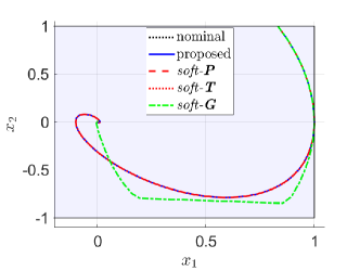
Figure 1: Closed-loop trajectories initialized at $x_{0}=c\cdot[0.832,1]^{\top}$ with $c=1$ (top), $c=1.520$ (middle), $c=4$ (top). The state constraint $\mathbb{X}$ is shaded. Infeasible MPC formulations are not plotted.

In case $c=1$, we have $x_{0}\in\mathbb{X}_{N}$ and as expected all formulations (approx.) satisfy the constraints. The proposed approach and the soft-constrained MPC formulations using an LQR based terminal penalty (soft-P, soft-T) are (approximately) equivalent to the nominal MPC on the feasible set. On the other hand, the globally feasible soft-constrained MPC (soft-G) requires a very large terminal penalty (factor $10^{6}$ larger) resulting in a significant performance deterioration.

We note that the soft-P approach looses feasibility for $c>1.02$. Hence, we directly consider $c=1.52$, on the boundary of the feasible set of soft-T. The soft-constrained MPC formulations soft-G and soft-T directly minimize the distance to the state constraints $\mathbb{X}$, which reduces the constraint violation by $5$–$8\%$. On the other hand, the proposed formulation achieves a better performance.

Considering the large initial condition with $c=4$, only the proposed approach and the soft-G implementation are feasible. In this case, the soft-G approach achieves better performance by using a bang-bang control, while the proposed approach has a smoother (and hence less performant) transition between applying the maximal and minimal input.

We note that the quantitative differences in the performance depend highly on the magnitude of the input regularization $R$.

The following table details the average relative computation times for the different MPC formulations evaluated on a $100\times 100$ grid over the feasible set $\mathbb{X}_{N}$.
nominal proposed soft-P soft-T soft-G $100\%$ $105.9\%$ $177.4\%$ $264.2.1\%$ $178.2\%$
As one may expect, the additional slack variables increase the computational demand of soft-constrained MPC schemes. Furthermore, the more complex terminal set for the soft-T approach further increases the complexity. On the other hand, the increased computational demand of the proposed relaxed initial state constraint is relatively small.

Summary

The overall complexity of the design and online optimization of the proposed approach is smaller or equal to the considered soft-constrained MPC alternatives. On the nominal feasible set $\mathbb{X}_{N}$, the proposed approach, soft-P and soft-T (approx.) recover the nominal MPC, while the soft-G approach resulted in a significant performance deterioration. For $x\notin\mathbb{X}_{N}$, the explicit penalty on constraint violations in soft-constrained MPC approaches can be tuned to achieve a smaller constraint violation, which is not directly possible in the proposed approach. For very large initial states (or equivalently outlier disturbances), only the proposed approach and soft-G are feasible, while the more direct cost in soft-G seems to result in a better performance. Overall, the proposed approach is the only method, which achieves both: local optimality and global stability; while in the soft-constrained MPC formulations either one of these properties is lost based on the choice of terminal penalty/set (soft-G vs. soft-P/T).

VII-B Nonlinear system subject to disturbances

With the following example, we demonstrate the practical benefits for nonlinear systems subject to large disturbances.

System model

We consider the four-tank system and the tracking MPC formulation from the experiments in [51, Sec. VI]. The system dynamics can be compactly written as:

$$\dot{x}_{1}= -c_{1}\sqrt{x_{1}}+c_{2}\sqrt{x_{2}}+c_{1,\mathrm{u}}u_{1},~{}~{}\dot{x}_{2}=-c_{2}\sqrt{x_{2}}+c_{2,\mathrm{u}}u_{2},$$

$$\dot{x}_{3}= -c_{3}\sqrt{x_{3}}+c_{4}\sqrt{x_{4}}+c_{3,\mathrm{u}}u_{2},~{}~{}\dot{x}_{4}=-c_{4}\sqrt{x_{4}}+c_{4,\mathrm{u}}u_{1},$$

with states $x\in\mathbb{R}_{\geq 0}^{4}$, inputs $u\in\mathbb{R}^{2}_{\geq 0}$, and positive constants $c_{i}>0$, $c_{i,\mathrm{u}}>0$, $i\in\mathbb{I}_{[1,4]}$. The input corresponds to the water flow, which is subject to the hard constraint $u\in\mathbb{U}=\{u\in\mathbb{R}^{2}_{\geq 0}|~{}u_{1}\leq 3.6,~{}u_{2}\leq 4\}$. The states correspond to the water level in different tanks and should ideally respect the constraints $x\in\mathbb{X}=\{x|~{}x_{i}\geq 0.2,~{}i\in\mathbb{I}_{[1,4]},~{}x_{i}\leq 1.36,i=1,3~{}x_{i}\leq 1.4,i=2,4\}$. The problem addresses a coupled multi-input-multi-output nonlinear open-loop stable system with non-minimum phase behaviour and constraints.

Open-loop stability

To implement the relaxed initial state constraint in Problem (7)/(29), we additionally compute an incremental Lyapunov function $V_{\delta}$ (Ass. 2) certifying open-loop stability. We consider a quadratic function $V_{\delta}(x,z)=\|x-z\|_{P}^{2}$ and hence it suffices to ensure $A^{\top}(x)P+PA(x)\prec 0$ (cf., e.g., [37, 34]) with the (continuous-time) Jacobian/linearization

$$A(x)=-0.5\begin{pmatrix}\tilde{c}_{1}&-\tilde{c}_{2}&0&0\\ 0&\tilde{c}_{2}&0&0\\ 0&0&\tilde{c}_{3}&-\tilde{c}_{4}\\ 0&0&0&\tilde{c}_{4}\end{pmatrix},\quad\tilde{c}_{i}=c_{i}x_{i}^{-0.5}.$$

Given the structure of the open-loop system, we consider the diagonal matrix $P=\text{diag}(1,p_{2},1,p_{4})$ and the stability condition reduces to

$$\begin{pmatrix}-2\tilde{c}_{1}&\tilde{c}_{2}\\ \tilde{c}_{2}&-2\tilde{c}_{2}p_{2}\\ \end{pmatrix}\prec 0,\quad\begin{pmatrix}-2\tilde{c}_{3}&\tilde{c}_{4}\\ \tilde{c}_{4}&-2\tilde{c}_{4}p_{4}\end{pmatrix}\prec 0.$$

The considered nonlinear physical model is only well-defined for $x_{i}\in(0,\infty)$ and hence open-loop stability (Ass. 2) and closed-loop properties cannot be shown globally for all $x\in\mathbb{R}^{n}$. Instead, we provide semi-global results in the sense that for each compact interval $x_{i}\in[\underline{x},\overline{x}]$, $i\in\mathbb{I}_{[1,4]}$, $0<\underline{x}\leq\overline{x}<\infty$, we can compute a suitable matrix $P$. Hence, we can ensure the provided closed-loop guarantees hold on an arbitrary large desired region of operation.

Simulation setup

As in [51, Sec. VI], we consider the problem of achieving a desired output $y=[x_{1},x_{3}]^{\top}\stackrel{{\scriptstyle!}}{{=}}y_{\mathrm{d}}=[1.3,1.3]^{\top}$, which is chosen on the boundary of the state constraints $\mathbb{X}$. We consider four MPC implementations: a nominal MPC implementation; an MPC implementation that relaxes the state constraints but keeps the terminal set constraint; the proposed formulation using a relaxed initial state constraint (Problem (7)); and the robust version thereof (Problem (29)). To assess the robustness, we consider uniformly distributed disturbances $\|w(k)\|_{\infty}\leq\overline{w}(k)$, where $\overline{w}(k)=0$ for $k\in\mathbb{I}_{[0,k_{1}]}$, then linearly increases up to $\overline{w}(k)=5\cdot 10^{-2}$ in $k\in\mathbb{I}_{[k_{1},k_{2}]}$, linearly decreases to $\overline{w}(k)=0$ in $k\in\mathbb{I}_{[k_{2},k_{3}]}$, and is again zero for $k\in\mathbb{I}_{[k_{3},k_{4}]}$ with $k_{i}\in\{50,250,450,550\}$. For the robustification w.r.t. small disturbances in Problem (29) we consider $\mathbb{W}=\{w|~{}\|w\|\leq 7\cdot 10^{-4}\}$, which is almost a factor $10^{2}$ smaller than the largest disturbances during the simulation.

The results can be seen in Figure 2. In the interval $k\in\mathbb{I}_{[0,k_{1}]}$ (no disturbances), we can see that the nominal MPC has a large region of attraction and successfully converges to the desired setpoint $y_{\mathrm{d}}$ on the boundary of the constraint set. As expected, the soft-constrained MPC and the proposed MPC using a relaxed initial state constraints are virtually indistinguishable from the nominal MPC in this nominal setting ($x\in\mathbb{X}_{N}$). In the interval $k\in\mathbb{I}_{[k_{1},k_{2}]}$, the magnitude of the disturbances $\overline{w}(k)$ increases linearly and the nominal MPC quickly becomes infeasible. Both the proposed MPC framework and the soft-constrained MPC result in trajectories with significant fluctuations and constraint violations. The soft-constrained MPC tends to achieve a smaller constraint violation, as one might expect due to the explicit penalty. Notably, despite the relaxation of the state constraints, the soft-constrained MPC has a bounded feasible set due to the required hard terminal constraints and the increasing magnitude of the disturbances $w$ results in a loss of feasibility. On the other hand, the proposed MPC framework retains feasibility irrespectively of the magnitude of the disturbances and the tracking error is proportional to the magnitude of the disturbances, as expected based on the theoretical analysis (Theorem 1).

Considering the robustified version of the proposed approach (Section V): Due to the tightened constraint set, the performance in the nominal case is worse, i.e., we do not reach the optimal steady-state on the boundary of the constraint set but keep a conservative distance. In the presence of disturbances, the constraint violations are significantly reduced (almost zero) and also the fluctuations seem to be smaller. In contrast to a conventional tube-based robust MPC design, the disturbance bound $\overline{w}$ considered in the proposed design (Sec. V) is a tuning variable that reduces constraint violations, but in general does not need to account for worst-case disturbances.

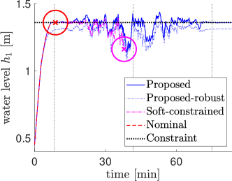
Figure 2: Closed-loop water level $h_{1}$ for different MPC formulations. State constraints and time points $k_{i}$, $i\in\mathbb{I}_{[1,4]}$, are shown as black dotted lines. The MPC schemes are stopped in case of infeasibility, which is highlighted with a circle with a cross $\times$.

Summary

We have demonstrated the practical benefits of the proposed MPC framework for nonlinear systems subject to disturbances. In the nominal case, both the proposed softened initial state constraint and the soft state constraints, approximately results in the same closed-loop trajectories as the nominal MPC scheme. In the presence of disturbances, classical soft-constrained MPC formulations may yield a smaller constraint violation. However, despite the large nominal feasible set $\mathbb{X}_{N}$ and the relaxation of the state constraints, standard soft-constrained MPC schemes may loose feasibility in the presence of large disturbances. On the other hand, the proposed relaxed initial state constraint ensures feasibility and (input-to-state) stability even under large disturbance. This makes the proposed approach particularly attractive in practice, as no infeasibility handling is required. Furthermore, the proposed robustification (Sec. V) allows for a flexible trade-off w.r.t. conservativeness and possible constraint violation, without affecting the stability and feasibility guarantees.

VIII Conclusion

For nonlinear open-loop stable systems, we showed that relaxing the initial state constraint in MPC with a suitable penalty provides a globally stabilizing formulation. The proposed approach can (approximately) recover the nominal MPC control law on the nominal feasible set, including the corresponding performance and constraint satisfaction properties. In case of large disturbances, the softened initial state constraint avoids loss of feasibility, ensures ISS w.r.t disturbances, and provides a suitable bound on the cumulative constraint violation. The proposed framework is particularly appealing in case of linear systems (Sec. VI) or as a relaxation of robust MPC formulations (Sec. V), since the penalty function $V_{\delta}$ is easy to design or already required in the robust design. The benefits of the proposed approach have been demonstrated using numerical examples (Sec. VII). Additionally, for exponentially open-loop stable systems, we showed how the overall implementation is facilitated using an implicit description of the penalty $V_{\delta}$ (Sec. IV), which may be of independent interest for the design of nonlinear robust MPC schemes (cf. Rk. 5).

-A Marginally stable systems and semi-global results

Many physical systems include integrators (e.g., kinematic problems), harmonic oscillators (i.e., without damping), or in general have some invariant quantities (e.g., energy). As such, these systems are at best marginally stable, i.e., Inequality (2) can only be satisfied with $\alpha_{\delta,3}=0$, and hence Theorem 1 is not applicable. Considering the corresponding proof, it is clear that $V_{\mathrm{slack}}$ remains a global Lyapunov function and hence the system state does not diverge in the absence of disturbances $w$. The following theorem shows that also (semi-global) asymptotic convergence/stability can be established.

Theorem 7.

Let Assumptions 1 and 3 hold with $\alpha_{i}(r)=c_{i}r^{2}$, $i\in\mathbb{I}_{[1,2]}$, $\alpha_{\ell}(r)=c_{\ell}r^{2}$, and $0\in\mathrm{int}(\mathbb{X}_{\mathrm{f}})$. Suppose further that there exists a matrix $P\succ 0$, such that $V_{\delta}(f(x,u),f(z,u))\leq V_{\delta}(x,z)$ for all $x,z\in\mathbb{R}^{n}$, $u\in\mathbb{U}$ with $V_{\delta}(x,z)=\|x-z\|_{P}^{2}$. Then, for any constant $\overline{V}>0$, there exists a constant $\lambda_{\overline{V}}>0$, such that for any $\lambda>\lambda_{\overline{V}}$ and any $x_{0}\in\mathbb{X}_{\mathrm{ROA}}=\{x\in\mathbb{R}^{n}|V_{\mathrm{slack}}(x)\leq\overline{V}\}$, the origin is exponentially stable for the closed-loop system (8) with $w(k)=0$, $k\in\mathbb{I}_{\geq 0}$.

Proof.

Note that $V_{\delta}$ satisfies Inequalities (2) with $\alpha_{1,\delta}(r)=\sigma_{\min}(P)r^{2}$, $\alpha_{2,\delta}=\sigma_{\max}(P)r^{2}$ and $\alpha_{3,\delta}=0$. Hence, $V_{\mathrm{slack}}$ is non-increasing using (11) and $\|w\|=0$, which implies that $x(k)\in\mathbb{X}_{\mathrm{ROA}}$ holds recursively. Furthermore, Inequalities (9a) remain true with $\tilde{\alpha}_{1}$ quadratic, i.e., $\tilde{\alpha}_{1}(r)=\tilde{c}_{1}r^{2}$. In the following, we use a case distinction based on whether $x\in\mathbb{X}_{N}$ to derive a lower bound on $\|x^{*}(x)\|$, which then implies exponential stability.
Part I: Consider $x\in\mathbb{X}_{N}$. Clearly, $V_{\mathrm{slack}}(x)\leq V_{\mathrm{norm}}(x)$ and hence

$$\lambda\sigma_{\min}(P)\|x-\overline{x}^{*}(x)\|^{2}\leq\lambda V_{\delta}(x,\overline{x}^{*}(x))\leq V_{\mathrm{nom}}(x)\leq c_{2}\|x\|^{2}.$$

Using the reverse triangle inequality, we arrive at

$$\|\overline{x}^{*}(x)\|\geq\|x\|-\|\overline{x}^{*}(x)-x\|\geq\left(1-\sqrt{\dfrac{c_{2}}{\lambda\sigma_{\min}(P)}}\right)\|x\|.$$

Part II: Consider $x\notin\mathbb{X}_{N}$. Given that $0\in\text{int}(\mathbb{X}_{N})$, there exists a constant $r>0$, such that $\|\overline{x}\|\leq r$ implies $\overline{x}\in\mathbb{X}_{N}$. Consider the candidate $\overline{x}=x\dfrac{r}{\|x\|}\in\mathbb{X}_{N}$, which satisfies $V_{\mathrm{nom}}(\overline{x})\leq\alpha_{2}(r)=c_{2}r^{2}$. Furthermore,

$$V_{\delta}(x,\overline{x})=\|x-\overline{x}\|_{P}^{2}=\left(1-\dfrac{r}{\|x\|}\right)^{2}V_{\delta}(x,0).$$

Note that $x\in\mathbb{X}_{\mathrm{ROA}}$, i.e., $V_{\mathrm{slack}}(x)\leq\overline{V}$, which implies

$$\tilde{c}_{1}\|x\|^{2}\stackrel{{\scriptstyle\eqref{eq:Lyap_joint_1}}}{{\leq}}V_{\mathrm{slack}}(x)\leq\overline{V}.$$ (34)

Hence, we get $\left(1-\dfrac{r}{\|x\|}\right)\leq 1-\dfrac{r\sqrt{\tilde{c}_{1}}}{\sqrt{\overline{V}}}=:\rho_{\overline{V}}\in(0,1)$. Using this feasible candidate solution, we have

$$\lambda V_{\delta}(x,\overline{x}^{*}(x))\leq V_{\mathrm{slack}}(x)\leq \lambda V_{\delta}(x,\overline{x})+V_{\mathrm{nom}}(\overline{x})$$

$$\leq \lambda\rho_{\overline{V}}^{2}V_{\delta}(x,0)+c_{2}r^{2}.$$ (35)

Applying Cauchy-Schwarz and Young’s inequality with some $\epsilon>0$ to the quadratic function $V_{\delta}$ yields

$$\|x\|_{P}^{2}\leq(1+\epsilon)\|x-\overline{x}^{*}(x)\|_{P}^{2}+\dfrac{1+\epsilon}{\epsilon}\|\overline{x}^{*}(x)\|_{P}^{2}.$$

This implies

$$\dfrac{1}{1+\epsilon}\|x\|_{P}^{2}-\dfrac{1}{\epsilon}\|\overline{x}^{*}(x)\|_{P}^{2}\leq\|x-\overline{x}^{*}(x)\|_{P}^{2}$$

$$\stackrel{{\scriptstyle\eqref{eq:semigloba_interm_2}}}{{\leq}} \rho_{\overline{V}}^{2}\|x\|_{P}^{2}+\dfrac{c_{2}}{\lambda}r^{2}.$$

Thus, we get

$$\|\overline{x}^{*}(x)\|_{P}^{2}\geq\epsilon\left(\dfrac{1}{1+\epsilon}-\rho_{\overline{V}}^{2}\right)\|x\|_{P}^{2}-\epsilon\dfrac{c_{2}r^{2}}{\lambda}.$$

Choosing $\epsilon=\dfrac{1-\rho_{\overline{V}}^{2}}{1+\rho_{\overline{V}}^{2}}>0$, we have $\dfrac{1}{1+\epsilon}-\rho_{\overline{V}}^{2}=\dfrac{1-\rho_{\overline{V}}^{2}}{2}>0$. Using additionally $\|x\|\geq r$, we get

$$\sigma_{\max}(P)\|\overline{x}^{*}(x)\|^{2}\geq\epsilon\dfrac{1-\rho_{\overline{V}}^{2}}{2}\|x\|_{P}^{2}-\epsilon\dfrac{c_{2}r^{2}}{\lambda}$$

$$\geq \epsilon\left(\dfrac{1-\rho_{\overline{V}}^{2}}{2}\sigma_{\min}(P)-\dfrac{c_{2}}{\lambda}\right)\|x\|^{2}.$$

Part III: Combing the results in Part I and II, we get

$$\|\overline{x}^{*}(x)\|^{2}\geq\epsilon_{\mathrm{V}}\|x\|^{2}\quad\forall x\in\mathbb{X}_{\mathrm{ROA}},$$

with $\epsilon_{\mathrm{V}}>0$ for $\lambda>\lambda_{\mathrm{V}}:=\dfrac{2c_{2}}{(1-\rho_{\mathrm{V}}^{2})\sigma_{\min}(P)}$. Using Inequality (11) with $\alpha_{3,\delta}=0$, $w=0$, and $\alpha_{\ell}$ quadratic, we arrive at

$$V_{\mathrm{slack}}(x^{+})-V_{\mathrm{slack}}(x)\leq -\alpha_{N}c_{\ell}\|\overline{x}^{*}(x)\|^{2}$$

$$\leq -\alpha_{N}c_{\ell}\epsilon_{\mathrm{V}}\|x\|^{2}.$$

Combining this bound with Inequalities (9a), we obtain exponential stability with the Lyapunov function $V_{\mathrm{slack}}$. ∎

This result ensures that for any compact set $\mathbb{X}_{\mathrm{RoA}}$, we can choose a large weight $\lambda$, such that the closed-loop system is exponentially stable. The result is semi-global in the sense that the value required for the weight $\lambda$ and the convergence rate deteriorate as $\overline{V}\rightarrow\infty$, which is in contrast to the uniform global guarantees in Theorem 1.

We expect that the restriction to quadratic functions $V_{\delta}$ can be relaxed by using the distance based on the Riemannian metric of general contraction metrics instead (cf. [37, 36]).

-B Nominal stabilizing MPC designs

In the following, we briefly elaborate on existing MPC design methods that ensure nominal stability on the feasible set, i.e., satisfy Assumption 3.

Most MPC designs utilize a local CLF $V_{\mathrm{f}}$ with a positive invariant terminal set $\mathbb{X}_{\mathrm{f}}\subseteq\mathbb{X}$ [35], i.e.,

$$\min_{u\in\mathbb{U}:f(x,u)\in\mathbb{X}_{\mathrm{f}}}V_{\mathrm{f}}(f(x,u))+\ell(x,u)\leq V_{\mathrm{f}}(x)\quad\forall x\in\mathbb{X}_{\mathrm{f}}.$$

A simple design for such a local CLF $V_{\mathrm{f}}$ is based on a local linearization [16], [1, Sec. 2.5.5]. Assuming $0\in\text{int}(\mathbb{X}_{\mathrm{f}})$, such a design satisfies Assumption 3 with $\alpha_{N}=1$ (cf. [1, Sec. 2.4.2]).

For MPC formulations without terminal ingredients ($\mathbb{X}_{\mathrm{f}}=\mathbb{R}^{n}$, $V_{\mathrm{f}}=0$), asymptotic stability can be ensured if $\mathbb{X}=\mathbb{R}^{n}$, an additional exponential cost-controllability holds, and a sufficiently large prediction horizon $N$ is chosen [2]. In this case, Assumption 3 holds with the suboptimality index $\alpha_{N}\in(0,1)$ and $\mathbb{X}_{N}=\mathbb{R}^{n}$.

The presented approach can be extended to the case where the recursive properties in Assumption 3 only hold on a sublevel set of the Lyapunov function $\mathbb{X}_{\mathrm{ROA}}=\{x\in\mathbb{X}_{N}|~{}V_{\mathrm{nom}}(x)\leq\overline{V}\}$, by explicitly including the constraint $\mathcal{J}_{N}(\overline{x},\mathbf{u})\leq\overline{V}$ in Problem (7). This generalization is relevant for the implicitly enforced terminal set constraints in [18]. This extension is also needed in MPC schemes without terminal penalty to handle the case of hard state constraints $\mathbb{X}$ [20].

In case the stage cost $\ell$ is not positive definite (Ass. 1), the value function $V_{\mathrm{nom}}$ is typically not a Lyapunov function and an additional storage function $W:\mathbb{R}^{n}\rightarrow\mathbb{R}_{\geq 0}$ is commonly added to obtain a Lyapunov function (cf. [19, 32], [1, Thm. 2.24]). In this case, the same storage function $W(\overline{x})$ is included in the cost function in (7) to ensure stability.

Johannes Köhler received his Master degree in Engineering Cybernetics from the University of Stuttgart, Germany, in 2017. In 2021, he obtained a Ph.D. in mechanical engineering, also from the University of Stuttgart, Germany, for which he received the 2021 European Systems & Control Ph.D. award. He is currently a postdoctoral researcher at the Institute for Dynamic Systems and Control (IDSC) at ETH Zürich. His current research interests are in the area of model predictive control and control and estimation for nonlinear uncertain systems.

Melanie N. Zeilinger is an Assistant Professor at ETH Zürich, Switzerland. She received the Diploma degree in engineering cybernetics from the University of Stuttgart, Germany, in 2006, and the Ph.D. degree with honors in electrical engineering from ETH Zürich, Switzerland, in 2011. From 2011 to 2012 she was a Postdoctoral Fellow with the Ecole Polytechnique Federale de Lausanne (EPFL), Switzerland. She was a Marie Curie Fellow and Postdoctoral Researcher with the Max Planck Institute for Intelligent Systems, Tübingen, Germany until 2015 and with the Department of Electrical Engineering and Computer Sciences at the University of California at Berkeley, CA, USA, from 2012 to 2014. From 2018 to 2019 she was a professor at the University of Freiburg, Germany. Her current research interests include safe learning-based control, as well as distributed control and optimization, with applications to robotics and human-in-the loop control.

References

- [1] J. B. Rawlings, D. Q. Mayne, and M. Diehl, Model Predictive Control: Theory, Computation, and Design. Nob Hill Publishing, 2017.
- [2] L. Grüne and J. Pannek, Nonlinear Model Predictive Control. Springer, 2017.
- [3] N. M. de Oliveira and L. T. Biegler, “Constraint handing and stability properties of model-predictive control,” AIChE J., vol. 40, no. 7, pp. 1138–1155, 1994.
- [4] A. Zheng and M. Morari, “Stability of model predictive control with mixed constraints,” IEEE Trans. Autom. Control, vol. 40, no. 10, pp. 1818–1823, 1995.
- [5] P. O. Scokaert and J. B. Rawlings, “Feasibility issues in linear model predictive control,” AIChE Journal, vol. 45, no. 8, pp. 1649–1659, 1999.
- [6] E. C. Kerrigan and J. M. Maciejowski, “Soft constraints and exact penalty functions in model predictive control,” in Proc. UKACC Int. Conf. on Control (CONTROL), 2000.
- [7] A. Richards, “Fast model predictive control with soft constraints,” European J. Control, vol. 25, pp. 51–59, 2015.
- [8] M. N. Zeilinger, M. Morari, and C. N. Jones, “Soft constrained model predictive control with robust stability guarantees,” IEEE Trans. Autom. Control, vol. 59, pp. 1190–1202, 2014.
- [9] K. P. Wabersich, R. Krishnadas, and M. N. Zeilinger, “A soft constrained MPC formulation enabling learning from trajectories with constraint violations,” IEEE Control Systems Letters, vol. 6, pp. 980–985, 2022.
- [10] S. V. Rakovic, S. Zhang, H. Sun, and Y. Xia, “Model predictive control for linear systems under relaxed constraints,” IEEE Trans. Autom. Control, 2021.
- [11] C. Feller and C. Ebenbauer, “Relaxed logarithmic barrier function based model predictive control of linear systems,” IEEE Trans Autom Control, vol. 62, no. 3, pp. 1223–1238, 2016.
- [12] J. B. Rawlings and K. R. Muske, “The stability of constrained receding horizon control,” IEEE Trans. Autom. Control, vol. 38, no. 10, pp. 1512–1516, 1993.
- [13] M. Sznaier and M. J. Damborg, “Suboptimal control of linear systems with state and control inequality constraints,” in Proc. IEEE Conf. Decision and Control (CDC), 1987, pp. 761–762.
- [14] D. Chmielewski and V. Manousiouthakis, “On constrained infinite-time linear quadratic optimal control,” Systems & Control Letters, vol. 29, no. 3, pp. 121–129, 1996.
- [15] P. O. Scokaert and J. B. Rawlings, “Constrained linear quadratic regulation,” IEEE Trans. Autom. Control, vol. 43, no. 8, pp. 1163–1169, 1998.
- [16] H. Chen and F. Allgöwer, “A quasi-infinite horizon nonlinear model predictive control scheme with guaranteed stability,” Automatica, vol. 34, pp. 1205–1217, 1998.
- [17] L. Grüne and A. Rantzer, “On the infinite horizon performance of receding horizon controllers,” IEEE Trans. Autom. Control, vol. 53, pp. 2100–2111, 2008.
- [18] D. Limon, T. Alamo, F. Salas, and E. F. Camacho, “On the stability of constrained MPC without terminal constraint,” IEEE Trans. Autom. Control, vol. 51, pp. 832–836, 2006.
- [19] G. Grimm, M. J. Messina, S. E. Tuna, and A. R. Teel, “Model predictive control: For want of a local control Lyapunov function, all is not lost,” IEEE Trans. Autom. Control, vol. 50, no. 5, pp. 546–558, 2005.
- [20] A. Boccia, L. Grüne, and K. Worthmann, “Stability and feasibility of state constrained MPC without stabilizing terminal constraints,” Systems & Control Letters, vol. 72, pp. 14–21, 2014.
- [21] S. Yu, M. Reble, H. Chen, and F. Allgöwer, “Inherent robustness properties of quasi-infinite horizon nonlinear model predictive control,” Automatica, vol. 50, pp. 2269–2280, 2014.
- [22] D. A. Allan, C. N. Bates, M. J. Risbeck, and J. B. Rawlings, “On the inherent robustness of optimal and suboptimal nonlinear MPC,” Systems & Control Letters, vol. 106, pp. 68–78, 2017.
- [23] D. Q. Mayne, M. M. Seron, and S. Raković, “Robust model predictive control of constrained linear systems with bounded disturbances,” Automatica, vol. 41, pp. 219–224, 2005.
- [24] D. Q. Mayne, E. C. Kerrigan, E. Van Wyk, and P. Falugi, “Tube-based robust nonlinear model predictive control,” Int. J. Robust and Nonlinear Control, vol. 21, pp. 1341–1353, 2011.
- [25] S. Singh, A. Majumdar, J.-J. Slotine, and M. Pavone, “Robust online motion planning via contraction theory and convex optimization,” in Proc. Int. Conf. Robotics and Automation (ICRA), 2017, pp. 5883–5890.
- [26] F. Bayer, M. Bürger, and F. Allgöwer, “Discrete-time incremental ISS: A framework for robust NMPC,” in Proc. European Control Conf. (ECC), 2013, pp. 2068–2073.
- [27] L. Hewing, K. P. Wabersich, and M. N. Zeilinger, “Recursively feasible stochastic model predictive control using indirect feedback,” Automatica, vol. 119, p. 109095, 2020.
- [28] L. Hewing and M. N. Zeilinger, “Stochastic model predictive control for linear systems using probabilistic reachable sets,” in Proc. Conference on Decision and Control (CDC), 2018, pp. 5182–5188.
- [29] H. Schlüter and F. Allgöwer, “Stochastic model predictive control using initial state optimization,” arXiv preprint arXiv:2203.01844, 2022.
- [30] J. Köhler and M. N. Zeilinger, “Recursively feasible stochastic predictive control using an interpolating initial state constraint,” IEEE Control Systems Letters, vol. 6, pp. 2743–2748, 2022.
- [31] Z.-P. Jiang and Y. Wang, “Input-to-state stability for discrete-time nonlinear systems,” Automatica, vol. 37, no. 6, pp. 857–869, 2001.
- [32] M. Diehl, R. Amrit, and J. B. Rawlings, “A Lyapunov function for economic optimizing model predictive control,” IEEE Trans. Autom. Control, vol. 56, pp. 703–707, 2011.
- [33] D. Angeli, “A Lyapunov approach to incremental stability properties,” IEEE Trans. Autom. Control, vol. 47, pp. 410–421, 2002.
- [34] D. N. Tran, B. S. Rüffer, and C. M. Kellett, “Convergence properties for discrete-time nonlinear systems,” IEEE Trans. Autom. Control, vol. 64, no. 8, pp. 3415–3422, 2019.
- [35] D. Q. Mayne, J. B. Rawlings, C. V. Rao, and P. O. Scokaert, “Constrained model predictive control: Stability and optimality,” Automatica, vol. 36, pp. 789–814, 2000.
- [36] I. R. Manchester and J.-J. E. Slotine, “Control contraction metrics: Convex and intrinsic criteria for nonlinear feedback design,” IEEE Trans. Autom. Control, vol. 62, pp. 3046–3053, 2017.
- [37] W. Lohmiller and J.-J. E. Slotine, “On contraction analysis for non-linear systems,” Automatica, vol. 34, pp. 683–696, 1998.
- [38] C. M. Kellett, “A compendium of comparison function results,” Mathematics of Control, Signals, and Systems, vol. 26, pp. 339–374, 2014.
- [39] G. Grimm, M. J. Messina, S. E. Tuna, and A. R. Teel, “Examples when nonlinear model predictive control is nonrobust,” Automatica, vol. 40, no. 10, pp. 1729–1738, 2004.
- [40] A. Casavola, M. Giannelli, and E. Mosca, “Global predictive regulation of null-controllable input-saturated linear systems,” IEEE Trans. Autom. Control, vol. 44, no. 11, pp. 2226–2230, 1999.
- [41] J. Köhler, “Analysis and design of MPC frameworks for dynamic operation of nonlinear constrained systems,” Ph.D. dissertation, Universität Stuttgart, 2021.
- [42] E. Rosenberg, “Exact penalty functions and stability in locally lipschitz programming,” Mathematical programming, vol. 30, no. 3, pp. 340–356, 1984.
- [43] D. Limon, T. Alamo, D. Raimondo, D. M. De La Peña, J. Bravo, A. Ferramosca, and E. Camacho, “Input-to-state stability: a unifying framework for robust model predictive control,” in Nonlinear Model Predictive Control: Towards New Challenging Applications. Springer, 2009.
- [44] D. Mayne, “Robust and stochastic model predictive control: Are we going in the right direction?” Annual Reviews in Control, vol. 41, pp. 184–192, 2016.
- [45] F. Blanchini, “Ultimate boundedness control for uncertain discrete-time systems via set-induced lyapunov functions,” IEEE Trans. Autom. Control, vol. 39, no. 2, pp. 428–433, 1994.
- [46] D. Q. Mayne, “Competing methods for robust and stochastic MPC,” in Proc. IFAC Conf. Nonlinear Model Predictive Control, 2018, pp. 169–174.
- [47] J. Lofberg, “YALMIP: A toolbox for modeling and optimization in matlab,” in Proc. IEEE Int. Symp. on Computed Aided Control Systems Design, 2004, pp. 284–289.
- [48] M. Herceg, M. Kvasnica, C. N. Jones, and M. Morari, “Multi-parametric toolbox 3.0,” in Proc. European control conference (ECC), 2013, pp. 502–510.
- [49] A. Wächter and L. T. Biegler, “On the implementation of an interior-point filter line-search algorithm for large-scale nonlinear programming,” Mathematical programming, vol. 106, no. 1, pp. 25–57, 2006.
- [50] J. A. Andersson, J. Gillis, G. Horn, J. B. Rawlings, and M. Diehl, “CasADi: A software framework for nonlinear optimization and optimal control,” Mathematical Programming Computation, vol. 11, no. 1, pp. 1–36, 2019.
- [51] D. Limon, A. Ferramosca, I. Alvarado, and T. Alamo, “Nonlinear MPC for tracking piece-wise constant reference signals,” IEEE Trans. Autom. Control, vol. 63, pp. 3735–3750, 2018.