Spotting Temporally Precise, Fine-Grained Events in Video

Abstract

We introduce the task of spotting temporally precise, fine-grained events in video (detecting the precise moment in time events occur). Precise spotting requires models to reason globally about the full-time scale of actions and locally to identify subtle frame-to-frame appearance and motion differences that identify events during these actions. Surprisingly, we find that top performing solutions to prior video understanding tasks such as action detection and segmentation do not simultaneously meet both requirements. In response, we propose E2E-Spot, a compact, end-to-end model that performs well on the precise spotting task and can be trained quickly on a single GPU. We demonstrate that E2E-Spot significantly outperforms recent baselines adapted from the video action detection, segmentation, and spotting literature to the precise spotting task. Finally, we contribute new annotations and splits to several fine-grained sports action datasets to make these datasets suitable for future work on precise spotting.

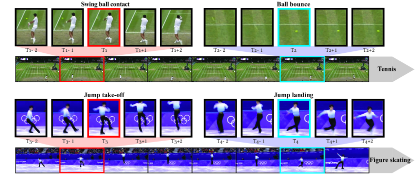
Figure 1: We perform temporally precise spotting of events in video, where success requires detecting the occurrence of an event within a single or small tolerance of frames. Examples of precise events: in tennis, the moment a player contacts the ball during a swing (red) or when a ball bounces on the court (blue); in figure skating, the moment of take-off (red) and landing (blue) during a jump.

1 Introduction

Detecting the precise moment in time events occur in a video (temporally precise event ‘spotting’) is an important video analysis task that stands to be essential to many future advanced video analytics and video editing [71] applications. However, despite significant progress in fine-grained video understanding [12, 31, 47, 62], temporal action detection (TAD) [5, 11, 30, 50, 67], and temporal action segmentation (TAS) [21, 32, 56], precise event spotting has rarely been studied by the video understanding community.

We address this gap by focusing on the challenge of precisely spotting events in sports video. We study sports video because of the quantity of data available and the high temporal accuracy needed to analyze human performances. For example, we wish to determine the frame in which a tennis player hits the ball, the frame a ball bounces on the court, or the moment a figure skater starts or lands a jump. Figure 1 shows examples from these sports and illustrates why precise spotting is challenging. The goal is to identify the precise frame when an event occurs, but adjacent frames are extremely similar visually; looking at one or two frames alone, it can be difficult even for a human to judge when a racket makes contact with a ball or when a figure skater lands a jump. However, inspection of longer sequences of frames makes the task significantly more tractable since the observer knows when to expect the event of interest in the context of a longer action (e.g., the swing of the racket, the preparation for a jump, or a ball’s trajectory). Therefore, we hypothesize that precise spotting requires models that can (1) represent subtle appearance and motion clues, and also (2) make decisions using information spread over long temporal contexts.

Surprisingly, we have found that the large body of literature on video understanding lacks solutions that meet these two requirements in the regime of temporally precise spotting. For example, action recognition (classification) models are not designed to operate efficiently on large temporal windows and struggle to learn in the heavily class-imbalanced setting created by precise spotting of rare events. Sequence models from segmentation and detection extract patterns over longer timescales, but training these complex models end-to-end has led to optimization challenges. This has resulted in many solutions that operate in two phases, relying on pre-trained (or modestly fine-tuned) input features that are not particularly specialized to capture the subtle (and often highly domain-specific) visual details needed to spot events with temporal precision.

We propose a simpler alternative (E2E-Spot) to satisfy our hypothesized requirements. The key to training a sequence model end-to-end over a wide temporal context is an efficient per-frame feature extractor that can process hundreds of contiguous frames without exceeding platform memory. We demonstrate how to combine existing modules from the video processing literature to accomplish this goal without introducing new, bespoke architectures.

Despite its simplicity, E2E-Spot significantly outperforms prior baselines, which opt for a two-phase approach, as well as naive end-to-end learning approaches on precise spotting. Moreover, E2E-Spot is computationally efficient at inference time and can complete the full end-to-end spotting task in less time than just the feature extraction phase of many prior methods [2, 6].

This paper makes three main contributions:

1. The novel task of temporally precise spotting of fine-grained events. We introduce frame-accurate labels for two existing fine-grained sports action datasets: Tennis [71] and Figure Skating [27]. We also adapt the temporal annotations from FineGym [47] and FineDiving [65] to show the generality of the precise spotting task.

2. E2E-Spot, a from-the-ground-up, end-to-end learning approach to precise spotting that combines well-established architectural components [8, 46, 57] and can be trained quickly on a single GPU.

3. Analysis of spotting performance. E2E-Spot outperforms strong baselines (§ 5) on precise temporal spotting (by 4–11 mAP, spotting within 1 frame). E2E-Spot is also competitive on coarser spotting tasks (within 1–5 sec), achieving second place in the 2022 SoccerNet Action Spotting challenge [13, 14] (within 1.1 avg-mAP) and a lift of 14.8–16.5 avg-mAP over prior work.

Our code and data are publicly available.

2 Related Work

Action Spotting.

Previous work on spotting [13] focuses on coarse action spotting, where a detection is deemed correct if it occurs within some time-window around the true event, with a loose error tolerance (1–5 or 5–60 seconds, equating to 10–100s of frames). On the Tennis [71] and Figure Skating [27] datasets described in § 4, a spotting error larger than 1–2 frames is essentially equivalent to missing the event altogether (e.g., a ball impact’s on the ground; Figure 1). For demanding applications that require precise temporal annotations, we argue the relevant task is precise event spotting, where detection thresholds are much more stringent tolerances (1–5 frames; as little as 33 ms in 25–30 FPS video). We use a similar metric to coarse action spotting: mean Average Precision (mAP @ $\delta$) but with a short temporal tolerance $\delta$.

Temporal Action Detection (TAD) and Segmentation (TAS)

localize intervals, often spanning several seconds and containing an ‘action’. Depending on the dataset, these can be atomic actions such as “standing up” [50] or broad activities such as “billiards” [30]. For such action definitions, it is often unclear what would be considered a temporally precise event to spot.

The success criteria for TAD and TAS also differ from that of precise spotting. TAD [5, 11, 30, 50, 67] is evaluated on interval-based metrics such as mAP @ temporal Intersection-over-Union (IoU) or at sub-sampled time points, neither of which enforce frame accuracy on the action boundaries. Down-sampling in time (up to 16$\times$) is a common preprocessing step [3, 38, 39, 48, 66, 70]. TAS [21, 32, 56] also optimizes interval-based metrics such as F1 @ temporal overlap. Frame-level metrics for TAS reward accuracy on densely labeled, intra-segment frames; in contrast, event frames in our spotting datasets are sparse. Spatial-temporal detection benchmarks [33, 35] differ from standard TAD, TAS, and precise spotting by combining both spatial and temporal IoU [35].

Recent approaches for TAD [10, 38, 39, 59, 66, 69] and TAS [1, 7, 20, 29, 53, 68] often proceed in two stages: (1) feature extraction then (2) head learning for the end task. Fixed, pre-trained features from video classification on Kinetics-400 are often used for the first stage [2, 6, 63], and state-of-the-art TAD methods with these features [41, 70, 73] often perform comparably to if not better than recent end-to-end learning approaches [36, 40]. Indirect fine-tuning using classification in the target domain is sometimes performed to improve feature encoding [2, 48]. Early end-to-end approaches encode video as non-overlapping segments [3] (e.g., 16 frames) or downsample in time [49, 51], producing features that are too temporally coarse to be effective for spotting frame-accurate events.

Like TAD and TAS, precise spotting is a temporal localization task performed on untrimmed video. As is the case, many models for TAD and TAS can be adapted for precise spotting. We use MS-TCN [20], GCN [66], GRU [8], and ASFormer [68] as baselines, and we test these models with different features [2, 6, 19] in § 5. However, we find that relying on fixed or indirectly fine-tuned features as input for these models is a critical limitation. Our experiments show that (1) E2E-Spot is a strong baseline for precise spotting and (2) more complex architectures do not necessarily provide additional benefit when feature learning is end-to-end. Finally, we note the long history of CNN-RNN architectures in TAD/TAS [3, 4, 52, 67, 16]; E2E-Spot is a simple design from this family, motivated by our requirements for frame-dense processing and end-to-end learning, and implemented using a modern CNN for spatial-temporal feature encoding.

Video Classification

predicts one label for an entire video, as opposed to per-frame labels for spotting. This leads to two key differences: (1) sparsely sampling frames [22, 63] is effective, whereas precise spotting requires dense sampling; (2) to obtain a video-level prediction, popular architectures for classification typically perform global space-time pooling [61] or temporal consensus [37, 63, 74]. E2E-Spot shows that omitting temporal pooling and training end-to-end yields an efficient pipeline for precise, per-frame spotting.

E2E-Spot incorporates ideas from popular video classification models for spatial-temporal feature extraction. TSM [37] introduced the temporal shift operation, which converts a 2D CNN into a spatial-temporal feature extractor by mixing channels between time steps. GSM [57] learns the shift. We find the combination of RegNet-Y [46] and GSM [57] to be effective and suggest these building blocks as a starting point for future spotting research.

Sports Activity Datasets

are a fertile testing ground for video action recognition and understanding [13, 25, 27, 28, 34, 35, 47, 65, 71]. We evaluate using temporal annotations from several recent datasets [13, 27, 47, 65, 71]. These datasets are fine-grained, meaning that all event and class labels relate to a single activity (i.e., a single sport), as compared to coarse-grained datasets [5, 30], where classes comprise a broad mix of generic activities. Supporting fine-grained concepts and labels is an important requirement of many practical, real-world applications.

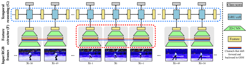
Figure 2: Overview of E2E-Spot. RGB video frames are first input to a local spatial-temporal feature extractor $F$ (a RegNet-Y [46] with GSM [57]) to produce a feature for each frame that captures subtle differences and motion across neighboring frames (red dotted box). The feature sequence is then processed by a sequence model $G$, which builds a long-scale temporal context (blue dotted box; one direction drawn) and outputs a class prediction for every frame.

3 E2E-Spot: An End-to-End Model for Precise Spotting

We define the precise temporal event spotting task as follows: given a video with $N$ frames $\mathbf{x}_{1},\ldots,\mathbf{x}_{N}$ and a set of $K$ event classes $\mathbf{c}_{1},\ldots,\mathbf{c}_{K}$, the goal is to predict the (sparse) set of frame indices when an event occurs, as well as the event’s class $(t,\hat{\mathbf{y}}_{t})\in\mathbb{N}\times\{\mathbf{c}_{1},\ldots,\mathbf{c}_{K}\}$. A prediction is deemed correct if its timestamp falls within $\delta$ frames of a labeled ground-truth event and it has the correct class label. In precise spotting, the temporal tolerance $\delta$ is small — i.e., a few frames only. We assume that the frame rate of the video is sufficiently high to capture the precise event and that frame rates are similar across videos.

We identified several key design requirements for a model to perform well on the temporally precise spotting task:

1. Task-specific local spatial-temporal features that capture subtle visual differences and motion across neighboring frames.

2. A long-term temporal reasoning mechanism, which provides a long temporal window to spot short, rare events. For instance, it is difficult to identify the precise time a figure skater enters a jump from a handful of frames. But spotting becomes much less ambiguous given the wider context of the acceleration (before) and landing (after the jump) (see Figure 1). These contexts can occur over many seconds and frames.

3. Dense frame prediction at the temporal granularity of a single frame.

These requirements call for an expressive and efficient network architecture that can be trained end-to-end via direct supervision on spotting.

E2E-Spot treats a video classification network (with global temporal pooling removed) as part of a sequence model, so that processing a clip of $N$ frames results in $N$ output features and $N$ per-frame predictions. Figure 2 illustrates our pipeline. Frames from each RGB video are first fed to a local spatial-temporal feature extractor $F$, which produces a dense feature vector for each frame (§ 3.1). This lightweight feature extractor incorporates Gate Shift Modules (GSM) [57] into a generic 2D convolutional neural network (CNN) [46]. The feature sequence is then further processed by a sequence model $G$, which builds a long-scale temporal context and outputs a class prediction for every frame, including a ‘background’ class to indicate when no event was detected (§ 3.2).

3.1 Local Spatial-Temporal Feature Extractor, $F$

The first stage of our pipeline extracts spatial-temporal features for each frame. We strive to keep the feature extractor as lightweight as possible, but found that a simple 2D CNN that processes frames independently [9, 23, 60, 63] is often insufficient for precise spotting (see § 5.2). This is because a 2D CNN does not capture the spatially-local temporal correlations between frames. In videos that are densely sampled (24–30 FPS), this temporal signal is critical to learn features that can robustly differentiate otherwise very similar frames: for instance, the speed and travel direction of a tennis ball, when each frame likely exhibits motion blur. To obtain more expressive, motion-sensitive features we implement $F$ as a 2D CNN with Gate Shift Modules (GSM) [57]. We choose RegNet-Y [46], a recent and compact CNN, as the 2D backbone.

Our feature extractor is similar to models for video classification [37, 57, 63], but with two key differences: (1) it samples frames densely and (2) it uses no final temporal consensus/pooling because our goal is to obtain one output per frame, rather than one for the whole video or multi-frame segment.

Efficiency Compared to Other Per-frame Feature Extractors.

A common alternative for per-frame feature extraction [2, 20] is to stride a video classification model densely — i.e., by using a model which takes $M$ frames as input and produces a single feature and by running it on the $M$ frame neighborhood of every frame. The overhead of processing each frame multiple times in overlapping windows makes end-to-end feature learning or fine-tuning difficult for tasks like spotting that require dense processing of frames. In contrast, our approach processes each frame once and can be trained as part of an end-to-end pipeline with much longer sequences (100s of frames), even on a single GPU (see Table 1).

3.2 Long-term Temporal Reasoning Module, $G$

To gather long-term temporal information, we use a 1-layer bidirectional Gated Recurrent Unit (GRU [8]) network $G$, which processes the dense per-frame features produced by $F$. We set the hidden dimension of $G$ to match that of $F$. Finally, we apply a fully connected layer and softmax on the GRU outputs to make a per-frame $K+1$ way prediction (including 1 ‘no-event’ background class).

We found that a single-layer GRU suffices and that more complex sequence models such as MS-TCN [20] or a deeper GRU do not necessarily improve accuracy (see § 5.2). We hypothesize that as a result of end-to-end training, the features produced by $F$ capture subtle temporal cues that are specific to a given activity’s and task’s requirements. This shifts the burden of representations to $F$ so that $G$ only needs to propagate the temporal context.

3.3 Per-frame Cross-Entropy Loss

For a $N$-frame clip, we output a sequence of $N$ class scores — i.e. a $(K+1)$-dimensional vector $\hat{\mathbf{y}}_{t}$ for each frame $t$, accounting for the background class:

$$(\hat{\mathbf{y}}_{1},\ldots,\hat{\mathbf{y}}_{N})=G\circ F(\mathbf{x}_{1},\ldots,\mathbf{x}_{N}).$$ (1)

Each frame has a ground-truth label $\mathbf{y}_{t}\in\{\mathbf{c}_{1},\ldots,\mathbf{c}_{K}\}\cup\{\mathbf{c}_{background}\}$ encoded as a one-hot vector. We optimize per-frame classification with cross-entropy loss:

$$l(\mathbf{x}_{1},\ldots,\mathbf{x}_{N})=\sum_{t=1}^{N}\operatorname{CE}(\hat{\mathbf{y}}_{t},\mathbf{y}_{t})$$ (2)

Table 1: E2E-Spot efficiency and throughput. We compare the model complexity, the maximum batch size for end-to-end training on 100 frame clips (at $224\times 224$), and per-frame inference time on a Nvidia A5000 GPU with 24GB of VRAM [44]. E2E-Spot is significantly faster at inferring features than striding a video classification model and allows for practical end-to-end trained spotting.

Architecture	Params (M)	Max batch size	Inference time (ms)
E2E-Spot: RegNet-Y 200MF w/ GSM + GRU	(2.8 + 1.7)	18	0.3
E2E-Spot: RegNet-Y 800MF w/ GSM + GRU	(5.5 + 7.1)	8	0.6
Comparison to other feature extractors: (* $:=$ exceeds GPU memory)
RegNet-Y 200MF w/ GSM (7 frames per window) 2.8		2	1.6
RegNet-Y 200MF w/ GSM (15 frames per window) 2.8		1	3.2
I3D (21 frames; used by [20])	12.3	*	8.5
R(2+1)D-34 [61] (12 frames, $128\times 128$; used by [2]) 63.7		*	11.0
ResNet-152 (1 frame only; used by [9, 23, 60])	60.2	2	1.8
Feature combination (for SoccerNet-v2) [75] $>$200		-	-

3.4 Implementation Details

We conduct experiments with two versions of $F$ utilizing RegNet-Y 200MF and 800MF (MF refers to MFLOPs [46]). These CNN backbones are initialized with pre-trained weights from ImageNet-1K [15]. Details of the complexity and throughput of these models is given in Table 1.

We train E2E-Spot on 100-frame-long clips sampled randomly and use standard data-augmentations (e.g., crop, jitter, and mixup [72]). Frames are resized to 224 pixels in height and cropped to $224\times 224$ unless otherwise stated (see Appendix 0.A). We optimize using AdamW [43] and LR annealing [42]. To mitigate imbalance arising from the rarity of precise events ($<3\%$ of frames), we boost the loss weight of the foreground classes (5$\times$) relative to the background.

At test time, we disable data-augmentation and overlap clips by 50%, averaging the per-frame predictions. To convert per-frame class scores into a set of spotting predictions, we rank all of the frames by their predicted score for each class. We follow standard procedure from coarse spotting [13] and other detection tasks [24] by reporting our results with non-maximum suppression (NMS). Empirically, we found NMS’s efficacy to vary by model and dataset (see Table 2). Refer to Appendix 0.A for more implementation details.

4 Datasets

We evaluate precise spotting on four fine-grained sports video datasets with frame-level labels: Tennis [71], Figure Skating [27], FineDiving [65], and FineGym [47]. For full details about these datasets, please refer to Appendix 0.D.

Tennis is an extension of the dataset from Vid2Player [71]. It consists of 3,345 video clips from 28 tennis matches (each clip is a ‘point’), with video frame rates of either 25 or 30 FPS. The dataset has 33,791 frame-accurate events divided into six classes: “player serve ball contact,” “regular swing ball contact,” and “ball bounce” (each divided by near- and far-court). Video from 19 matches are used for training and validation, while 9 matches are held out for testing.

Figure Skating [27] consists of 11 videos (all 25 FPS) containing 371 short program performances from the Winter Olympics (2010–2018) and World Championships (2017–2019). We refine the original labels by manually (re-)annotating the take-off and landing frames of jumps and flying spins, resulting in 3,674 event annotations across four classes. We consider two splits for evaluation:

• Competition split (FS-Comp): holds out all videos from the 2018 season for testing [27]. This split tests generalization to new videos (e.g., the next Olympics), despite domain-shift such as a new background in a new venue.

• Performance split (FS-Perf): stratifies each competition across train / val / test. This split tests a model’s ability to learn precise temporal events (by different skaters) without the background bias of the previous split.

FineDiving [65] contains 3,000 diving clips with temporal segment annotations. We spot the step transition frames for four classes, which include transitions into somersaults (pike and tuck), twists, and entry.

FineGym [47] contains 5,374 gymnastics performances, each treated as an untrimmed video. It has 32 spotting classes, derived from a hierarchy of action categories (e.g., balance beam dismounts; floor exercise turns). The original annotations denote the start and end of actions; we treat these boundaries as events — for instance, “balance beam dismount start” and “balance beam dismount end”. We ignore the original splits, which are designed for action recognition and have overlap in videos, and we propose a 3:1:1 split between train / val / test. To reduce the variation in the frame rates of the source videos (which are 25–60 FPS), we resample all 50 and 60 FPS videos to 25 and 30 FPS, respectively.

Upon inspecting the FineGym labels for frame accuracy, we found the annotations for action start frames to be more visually consistent than those for end frames. For example, unlike in the Figure Skating dataset, the end frame is often several frames after the frame of landing for a jump. Thus, we also report results for a subset, FineGym-Start, which contains only start-of-action events.

5 Evaluation

In § 5.1, we demonstrate that the quality of per-frame feature representations extracted from the video has the greatest impact on results, rather than the choice of head architecture, and that end-to-end learning with E2E-Spot outperforms methods using pre-trained or indirectly fine-tuned features. In § 5.2 and § 5.3 we analyze the effect of temporal context, the importance of temporal modeling, and additional variations of E2E-Spot. In  § 5.4 we report results on SoccerNet-v2, a temporally coarser spotting task.

Evaluation Metric.

We measure Average Precision within a tolerance of $\delta$ frames (AP @ $\delta$). AP is computed for each event class, and mAP is the mean across classes. We focus on tight tolerances such as $\delta=1$ and $\delta=2$. Precise temporal events are rare as a percentage of frames (0.2–2.9%), so metrics such as frame-level accuracy are not meaningful for precise spotting.

Baselines.

We evaluate E2E-Spot against recent baselines from TAS, TAD, and coarse spotting that we adapted to the precise spotting task. These methods are not trained end-to-end; they adopt a two-phase separation between feature extraction and head training (i.e., downstream model) for the end-task. We form our baselines by pairing a feature extraction strategy with a spotting head. The latter is trained on extracted features to perform precise spotting, using the per-frame loss from Equation 2. See Appendix 0.B for implementation details.

The baselines use the following head architectures: MS-TCN [20], GRU [8], ASFormer [68] from TAS; GCN [66] from TAD; and NetVLAD++ [23] and transformer [75] from action spotting. MS-TCN, GRU, and ASFormer performed best in our experiments, so we relegate results from the remaining architectures to § 0.C.1. We further attempt to boost the performance of these baselines using additional losses from the spotting literature, such as CALF [9] and label dilation, and by post-processing using non-maximum suppression (within $\pm 1$ frames). We report results from the best configuration of each baseline.

We pair each head architecture with pre-extracted input features, grouped into three broad categories:

1. Pre-trained features from video classification on Kinetics-400 [31], which are often used without any fine-tuning for TAD and TAS. Like Farha et al. [20], we extract per-frame I3D features by densely striding a 21-frame window around each frame. To test the impact of better pre-trained models, we also extract features with MViT-B [19], a state-of-the-art model from 2021.

2. Fine-tuned features using TSP [2] and ($K$ + 1)-way clip classification. These features come from a classifier trained to predict whether a small window (e.g., 12 frames) contains an event, and they have the benefit of being adapted to the target video domain (e.g., tennis, skating, gymnastics).

3. Pose features (VPD) for the Figure Skating dataset only, which utilize a hand-engineered pipeline for subject tracking and fine-tuning [27]. These features utilize domain-knowledge and are costly to develop for new datasets, which may include phenomena not captured by pose (e.g., ball bounce in tennis). In activities such as figure skating, defined heavily by human motion, VPD features serve as a ceiling for E2E-Spot, which is domain agnostic.

Finally, we add a naive, end-to-end learned baseline that adapts video classification directly to the spotting task (VC-Spot). VC-Spot is given a 15-frame clip and tasked to predict whether the middle frame is a precise event. This baseline is to show that precise spotting is a distinct task from video classification.

Table 2: Spotting performance (mAP @ $\delta$ frames). The top results in each category and each column are underlined. SOTA is bold. We report best results under the following: † indicates NMS; * indicates CALF [9] or dilation. (e) E2E-Spot, trained with RGB only, generally outperforms the non-pose baselines and is competitive with the pose baselines on Figure Skating. E2E-Spot can further be improved with a larger 800MF CNN and a 2-stream ensemble with flow.

Tennis

FS-Comp

FS-Perf

FineDiving

FG-Full

FG-Start

Feature

Model

$\delta$=1

2

1

2

1

2

1

2

1

2

1

2

(a) Pre-trained features (from Kinetics-400)

I3D [6]

MS-TCN

62.7

†*75.4

60.8

†*79.5

*69.0

†*89.3

-

-

-

-

-

-

(RGB & flow)

GRU

†*45.7

†*70.5

*41.8

†*69.8

*52.5

†*77.5

-

-

-

-

-

-

ASFormer

*58.1

†*76.5

*61.2

†*82.4

69.0

†*89.7

-

-

-

-

-

-

MViT-B [19]

MS-TCN

67.0

†*80.1

*57.4

†*79.9

*64.8

†*84.3

*59.3

†*78.3

†31.0

†*48.6

†41.7

†*64.8

(RGB)

GRU

64.8

†*80.8

45.6

†*73.1

56.8

†*79.1

57.3

76.7

†*28.5

†*48.6

†*39.1

†*62.2

ASFormer

*63.9

†79.9

55.8

†*81.8

*56.5

†*81.7

*38.5

†*67.4

†*25.3

†*42.9

†*32.5

†*55.3

(b) Fine-tuned features

TSP [2]

MS-TCN

*90.9

†*95.1

72.4

†*87.8

*76.8

*89.9

*57.7

†76.0

†40.5

†58.5

†53.9

†*73.5

(RGB)

GRU

89.5

†*96.0

*68.4

†*88.3

75.5

†*90.6

*57.0

*78.2

†*38.7

†*58.8

†*53.2

†*74.2

ASFormer

89.8

†*95.5

77.7

†94.1

80.2

†94.5

*51.3

†*77.4

†38.8

†57.6

†51.1

†*72.9

($K$ + 1)-VC

MS-TCN

91.1

†*95.1

66.5

†77.2

*77.2

†*89.9

63.2

†*83.5

†40.9

†*58.2

†53.2

†*73.8

(RGB)

GRU

†*91.5

†*96.2

†*61.7

†*78.9

†*76.8

†*89.4

*61.8

†*82.6

†41.1

†57.9

†54.3

†*73.6

ASFormer

92.1

†*96.2

*67.6

†*79.8

77.1

†*89.8

*58.9

†*83.5

†40.0

†*56.9

†*53.6

†*72.9

(c) Hand-engineered tracking & pose features (top scores shown; see § 0.C.1 for GRU and ASFormer)

2D-VPD [27]

MS-TCN

-

-

*83.5

†*96.2

*85.2

†*96.4

-

-

-

-

-

-

(d) VC-Spot: video classification baseline using RGB

RegNet-Y 200MF w/ GSM

†92.4

†96.0

†61.8

†75.5

†56.2

†75.3

†62.4

†85.6

†18.7

†28.6

†25.9

†38.3

(e) E2E-Spot

Default: 200MF (RGB)

96.1

†97.7

†*81.0

†*93.5

†*85.1

†*95.7

68.4

†85.3

†47.9

†65.2

†61.0

†78.4

Best: 800MF (2-stream)

†96.9

†98.1

†*83.4

†*94.9

†*83.3

†*96.0

†66.4

†84.8

†51.8

†68.5

†65.3

†81.6

Table 3: Ablation and analysis experiments (mAP @ $\delta=1$). We compare to E2E-Spot defaults in the top row (RegNet-Y 200MF w/ GSM and GRU). (a) Varying clip lengths show that temporal context from longer clips is generally helpful. (b) Removing temporal information in the feature extractor $F$ (GSM) and in the stateful predictions $G$ (GRU) generally reduces mAP. (c) Reducing input resolution from 224 to 112 pixels reduces mAP. (d) More complex models for $G$ than the 1-layer GRU do not significantly improve mAP. (e) Enlarging $F$ to 800MF and/or adding flow can improve mAP slightly on some datasets.

		Tennis		FS-Comp		FS-Perf		FineDiving		FineGym-Full
Experiment		mAP	$\Delta$	mAP	$\Delta$	mAP	$\Delta$	mAP	$\Delta$	mAP	$\Delta$
E2E-Spot default: clip length = 100		96.1		†81.0		†85.1		68.4		†47.4
(a)	clip length = 8	†95.8	$-0.3$	†73.7	$-7.3$	†74.7	$-10.4$	†67.3	$-1.1$	†32.3	$-15.1$
	clip length = 16	†96.2	$+0.1$	†74.4	$-6.6$	†80.1	$-5.0$	†64.8	$-3.6$	†40.8	$-6.6$
	clip length = 25	†96.2	$+0.1$	†74.5	$-6.5$	†80.6	$-4.5$	†67.2	$-1.2$	†43.9	$-3.5$
	clip length = 50	†96.4	$+0.3$	†76.9	$-4.1$	†82.3	$-2.8$	65.0	$-3.4$	†46.6	$-0.8$
	clip length = 250	96.4	$+0.3$	†81.3	$+0.3$	†85.6	$+0.5$	68.9	$+0.5$	†48.5	$+1.1$
	clip length = 500	95.9	$-0.2$	†78.9	$-2.1$	†87.5	$+2.4$	-	-	†48.1	$+0.7$
(b)	w/o GRU	†95.7	$-0.4$	†74.3	$-6.7$	†77.9	$-7.2$	64.1	$-4.3$	†32.9	$-14.5$
	w/ TSM [37] instead of GSM	96.1	$+0.0$	†78.6	$-2.4$	†83.3	$-1.8$	†65.3	$-3.1$	†48.1	$+0.7$
	w/o GSM	†94.1	$-2.0$	†75.5	$-5.5$	†85.6	$+0.4$	68.9	$+0.5$	†44.2	$-3.2$
	w/o GSM & GRU	†60.1	$-36.0$	†26.9	$-54.1$	†41.1	$-44.0$	†47.0	$-21.4$	†22.1	$-25.3$
(c)	w/ 112 px resolution (height)	†88.5	$-7.6$	†75.4	$-5.6$	†80.9	$-4.2$	†64.9	$-3.5$	†45.3	$-2.6$
(d)	w/ MS-TCN	95.7	$-0.4$	†77.6	$-3.4$	†84.7	$-0.4$	67.0	$-1.4$	†44.1	$-3.3$
	w/ ASFormer	95.7	$-0.4$	†68.4	$-12.6$	†75.4	$-9.7$	70.4	$+2.0$	†36.8	$-10.6$
	w/ Deeper GRU	96.5	$+0.4$	†80.2	$-0.8$	†83.5	$-1.6$	67.2	$-1.2$	†46.4	$-1.0$
	w/ GRU* (see supplement)	96.2	$+0.1$	†78.1	$-2.9$	†86.0	$+0.9$	67.4	$-1.0$	†47.9	$+0.5$
(e)	200MF (Flow)	†58.2	$-37.9$	†72.4	$-8.6$	†76.6	$-8.5$	†60.7	$-7.7$	†44.4	$-3.0$
	200MF (RGB + flow; 2-stream)	†96.3	$+0.2$	†82.2	$+1.2$	†85.1	$+0.0$	†70.1	$+1.7$	†49.0	$+1.6$
	800MF (RGB)	96.8	$+0.7$	†84.0	$+3.0$	†83.6	$-1.5$	64.6	$-3.8$	†50.1	$+2.7$
	800MF (Flow)	†59.2	$-36.9$	†74.9	$-6.1$	†74.2	$-10.9$	†59.8	$-8.6$	†46.9	$-0.5$
	800MF (RGB + flow; 2-stream)	†96.9	$+0.8$	†83.4	$+2.4$	†83.3	$-1.8$	†66.4	$-2.0$	†51.8	$+4.4$

5.1 Spotting Performance

We present two variations of E2E-Spot in the main results: (1) a default configuration with a RegNet-Y [46] 200MF CNN backbone and RGB input only, and (2) a configuration using RegNet-Y 800MF with RGB and flow input.

E2E-Spot with a 200MF CNN and RGB inputs consistently outperforms all non-pose baselines, while being comparable to the pose ones. The benefits of E2E-Spot are most striking at the most stringent tolerance, $\delta=1$ frame (Table 2e). We summarize the key takeaways of our evaluation below.

Pre-trained features generalize poorly when no fine-tuning is used, regardless of the head architecture: between 9.1–29.1 worse than E2E-Spot in mAP at $\delta=1$ (Table 2a). Fine-tuning yields a significant improvement over pre-trained features: between 3.9–25.1 mAP at $\delta=1$ (Table 2b), indicating a large domain gap between Kinetics and the fine-grained spotting datasets. However, E2E-Spot further outperforms the two-phase approaches with fine-tuned features by 3.3–6.8 mAP, showing that indirect fine-tuning strategies for temporal localization tasks should be compared against directly supervised, end-to-end learned baselines. Finally, the wide variation in baseline performance (by sport) highlights the importance of evaluating new tasks, such as precise spotting, and their methods on a visually and semantically diverse set of activities and datasets.

VC-Spot performs poorly compared to E2E-Spot (Table 2d), especially on Figure Skating and FineGym, which require temporal understanding at longer timescales (e.g., several seconds) compared to Tennis and FineDiving.

E2E-Spot achieves similar results to pose features (2D-VPD [27]) on Figure Skating, within 0.1–2.5 mAP at $\delta=1$. This is encouraging because E2E-Spot assumes no domain knowledge and is a more generally applicable approach.

Table 2e also shows E2E-Spot’s best configuration, using the larger 800MF CNN and both RGB and flow [58]. Neither of these enhancements (e.g., a larger CNN or flow) require domain knowledge, but can provide a small boost to the final performance over our 200MF defaults (0.8 mAP on Tennis and 3.9–4.3 mAP on FineGym). Details for other E2E-Spot configurations are presented in § 5.3.

5.2 Ablations of E2E-Spot

We analyze the requirements of precise spotting with respect to temporal context and network architecture. Refer to Appendix 0.C for additional ablations.

Sensitivity to Clip Length.

As a sequence model, E2E-Spot can benefit from and make stateful predictions over a long temporal context (e.g., 100s of frames). A long clip length allows for greater temporal context for each prediction, but linearly increases memory utilization per batch. We consider the number of frames needed for peak accuracy and train E2E-Spot with different clip lengths. Table 3a shows that different activities require different amounts of temporal context; the fast-paced events in Tennis can be successfully detected even when context is only 8–16 frames. In contrast, Figure Skating and FineGym show a clear drop in performance when clip length is reduced from 100 frames. Even longer clip lengths may be desirable (e.g., 250 frames), though with diminishing returns.

Value of Temporal Information in the Per-frame Features.

E2E-Spot incorporates temporal information both in the 2D CNN backbone $F$ (with GSM) and after global spatial-pooling in $G$ (with GRU). We show the criticality of both of these components in Table 3b at $\delta=1$. With neither GSM nor the GRU, the spotting task becomes a single-image classification problem; as expected, the results are poor (at least $-21$ mAP). The best results are achieved with both GSM and the GRU, except on FS-Perf and FineDiving, where results with and without GSM are similar. Replacing GSM with TSM [37] (fixed shift) ranges from comparable to worse, showing GSM to be a reasonable starting default.

Spatial Resolution.

Lowering spatial resolution [36, 40] can speed up end-to-end learning and inference but degrades mAP on precise spotting (Table 3c), where the subjects may, at times, occupy only a small portion of the frame.

5.3 Additional Variations of E2E-Spot

More Complex Architectures, $G$.

Prior TAD and TAS works catalog a rich history of head architectures (see related; § 2) operating on pre-extracted features. We examine whether these architectures can directly benefit from end-to-end learning with E2E-Spot by replacing the 1-layer GRU. Table 3d shows that improvement is not guaranteed; MS-TCN, ASFormer, and deeper GRUs neither consistently nor significantly outperform a single layer GRU. This suggests that end-to-end learned spatial-temporal features can already capture much of the logic previously handled by the downstream architecture.

Enhancements to Feature Extractor, $F$.

We explore two basic enhancements to $F$ that do not require new assumptions or domain knowledge: a larger CNN backbone (such as RegNet-Y 800MF) and optical flow [58] input. Table 3e shows that these enhancements can yield modest improvements (up to 4.4 mAP on FineGym). Flow, by itself, is worse than RGB but can improve results when ensembled with RGB. Larger models show promise on some datasets, but the improvements are not as significant as the lift from end-to-end learning.

5.4 Results on the SoccerNet Action Spotting Challenge

Table 4: Average-mAP @ $t$ for tolerances in seconds. SOTA in bold. We show the top results from the CVPR 2021 and 2022 SoccerNet Action Spotting challenges. ‡ indicates challenge results — trained on the train, validation, and test splits. Shown and unshown refer to whether actions are visible; E2E-Spot is better at detecting the former, but Soares et al. [54] is superior at the latter.

	Test split		Challenge split
Average-mAP @ tolerances	Tight (1–5 s)	Loose (5–60 s)	Tight (1–5 s)	Shown	Unshown
RMS-Net [60]	28.83	63.49	27.69	-	-
NetVLAD++ [23] -		-	43.99	-	-
Zhou et al. [75] (2021 challenge; 1st)	47.05	73.77	49.56	54.42	45.42
‡Soares et al. [54] (2022 challenge; 1st) -		-	‡67.81	‡72.84	‡60.17
E2E-Spot 200MF	61.19	73.25	63.28	70.41	45.98
E2E-Spot 800MF	61.82	74.05	66.01	72.76	51.65
‡E2E-Spot 800MF (2022 challenge; 2nd) -		-	‡66.73	‡74.84	‡53.21

E2E-Spot also generalizes to temporally coarse spotting tasks, such as SoccerNet-v2 [13], which studies 17 action classes in 550 matches — split across train / val / test / challenge sets. As in prior work [9, 23, 60], we extract frames at 2 FPS and evaluate using average-mAP across tolerances, defined as $\pm\delta/2$ second ranges around events. In Table 4, we compare E2E-Spot to the best results from the CVPR 2021 (lenient tolerances of 5–60 sec) and CVPR 2022 (less coarse, 1–5 sec tolerances) SoccerNet Action Spotting challenges [14].

E2E-Spot, with the 200MF CNN, matches the top prior method from the 2021 competition [75] in the 5–60 sec setting while outperforming it by 13.7–14.1 avg-mAP points in the less coarse, 1–5 sec setting. Increasing the CNN to 800MF improves avg-mAP slightly (by 0.4–2.7 avg-mAP). E2E-Spot places second in the (concurrent) 2022 competition (within 1.1 avg-mAP), after Soares et al. [54], due to the latter’s strong performance on unshown actions (not visible in the frame). Soares et al. [55, 54] and Zhou et al. [75] are two-phase approaches, combining pre-extracted features from multiple (5 to 6) heterogeneous, fine-tuned feature extractors and proposing downstream architectures and losses on those features. In contrast, E2E-Spot shows that direct, end-to-end training of a simple and compact model can be a surprisingly strong baseline.

6 Discussion and Future Work

In this paper, we have presented a from-the-ground-up study of end-to-end feature learning for spotting in the temporally stringent setting.

E2E-Spot is a simple baseline that obtains competitive or state-of-the-art performance on temporally precise (and coarser) spotting tasks, outperforming conventional approaches derived from related work on TAD and TAS (§ 2). The secondary benefits we obtain from end-to-end learning are a simplified analysis pipeline, trained in a single phase under direct supervision, and the ability to use smaller, simpler models, without sacrificing accuracy on the frame-accurate task. Methodological enhancements such as improved architectures (e.g., based on ViT [17]) for feature extraction, training methodologies, head architectures, and losses that benefit from end-to-end learning are interesting research directions. We hope that E2E-Spot serves as a principled baseline for this future work.

Video understanding encapsulates a broad body of tasks, of which spotting frame-accurate events is a single example. We consider it future work to analyze other tasks and their datasets, and we anticipate situations where end-to-end learning alone may be insufficient: e.g., when reliable priors such as pose are readily available, or when training data is limited or exhibits domain-shift in the pixel domain. Learning to spot accurately with few or weak labels will accelerate the curation new datasets for more advanced, downstream video analysis tasks.

7 Conclusion

We have introduced temporally precise spotting in video, supported by four fine-grained sports datasets. Many recent advances in TAD, TAS, and spotting trend towards increasingly complex models and processing pipelines, which generalize poorly for this strict, but practical setting. E2E-Spot shows that a few key design principles — task-specialized spatial-temporal features, reasoning over sufficient temporal context, and efficient end-to-end learning — can go a long way for improving accuracy and simplifying solutions.

Acknowledgements.

This work is supported by the National Science Foundation (NSF) under III-1908727, Intel Corporation, and Adobe Research. We also thank the anonymous reviewers for their comments and feedback.

Appendix 0.A Implementation Details for E2E-Spot

0.A.1 Spatial-Temporal Feature Extractor, $F$

As described in § 3, our feature extractor is a standard RegNet-Y [46] with Gate Shift Modules [57] (GSM) inserted. GSM is applied at each residual block, to $\frac{1}{4}$ of the channels, rounded up to the nearest multiple of 4. RegNet-Y 200MF and 800MF produce spatially-pooled features of dimension 368 and 768 respectively.

We choose RegNet-Y [46] over the more commonly used ResNet [26] family of 2D CNNs because the former is more recent and compact (RegNet-Y 200MF has 3.2M parameters vs. 11.7M parameters for ResNet-18), while exhibiting generally better performance on image classification benchmarks [64]. E2E-Spot, however, can be implemented with any 2D CNN architecture.

0.A.2 Long-term Temporal Reasoning Module, $G$

$G$ provides temporal reasoning on dense feature vectors, following the spatial pooling layer of $F$. The details of $G$ are given in the paper in § 3.2. Here, we provide details for the additional variations of E2E-Spot used in § 5.3.

Deeper GRU increases the number of GRU layers to 3. MS-TCN and ASFormer are described in § 0.B.1.

GRU* takes multiple 1-layer GRUs at different temporal granularities, in addition to the 1-layer GRU, to more directly aggregate information across wider contexts. We use two temporal scales, 4 and 16, requiring two additional GRUs. Each scale defines a temporal down-sampling of the clip length by a factor of the scale, $S$. For each scale, all output features are first fed to a fully connected layer and ReLU. Then, the sequence of length $N$ is divided into $\lceil\frac{N}{S}\rceil$ non-overlapping windows, and max-pooling is performed in each window. The $\lceil\frac{N}{S}\rceil$ sequence is processed by the scale-specific GRU. Finally, the outputs of each GRU, at each time scale, are up-sampled by repetition back to the full clip length $N$ and concatenated for each time step $t$.

While these experiments do not cover the full breadth of architectures and settings available, we note that we did not observe major performance gains over the 1-layer GRU in applying these alternatives alongside end-to-end learning.

0.A.3 Training Configuration

We train E2E-Spot using 100 frame long clips by default and a batch size of 8 clips. Batches are formed by randomly sampling clips from the training videos. We group every 625 training steps into a training cycle (i.e., a pseudo-epoch of 500K frames). A single cycle runs in approximately 8.5 and 14 minutes on a single A5000 GPU [44] for the 200MF and 800MF variants, respectively. All variations of E2E-Spot are trained for 50 cycles on the Tennis, Figure Skating, and FineDiving datasets. We train the 200MF model for 100 cycles and the 800MF model for 150 cycles on FineGym and SoccerNet-v2, due to the larger dataset sizes (see Appendix 0.D). Training is performed with AdamW [43], setting a base learning rate of $10^{-3}$, with 3 linear warmup cycles followed by cosine decay [42].

Data Augmentations.

We randomly apply color jitter, Gaussian blur, and mixup [72] during training. On Tennis, Figure Skating, and FineGym, we also randomly crop the $398\times 224$ frames to $224\times 224$ pixels. This crop only affects the width dimension, as cropping the height dimension can lead to precise events falling outside the visible field (e.g., the tennis court and player span the vertical dimension). For FineDiving [65], we use the frames extracted by the original authors (256 pixels in the vertical dimension) and random crops of $224\times 224$ pixels. Finally, for SoccerNet-v2, we do not use random cropping because context such as the goal or the field boundary are often at the periphery of the frame.

For Figure Skating only (FS-Perf and FS-Comp), we use label dilation of $\pm 1$ frames due to the very large imbalance between events and background frames (see § 0.D.2). Label dilation is beneficial on Figure Skating for both E2E-Spot and the baselines (see § 0.C.2). Note that label dilation is not used during testing.

Non-maximum Suppression.

We evaluated the model predictions with and without non-maximum suppression (NMS). For the temporally precise datasets, we used a window of $\pm 1$ frames whereas we use $\pm 2$ frames at 2 FPS for SoccerNet-v2. The efficacy of NMS in the temporally precise setting depends on the frame level tolerance, dataset, and model (see experiments in § 0.C.3), so the decision to apply NMS in practice should be made with application and task requirements in mind.

0.A.4 Optical Flow Extraction, for Additional Experiments

We use optical flow extracted by RAFT [58] for the additional 2-stream experiments that we described in § 5.3. During preprocessing, we subtract the median flow value for each frame and clamp to a range of $[-20,+20]$ pixels.

Appendix 0.B Implementation Details for Baselines

We adapt a number of published architectures from the action segmentation (TAS), detection (TAD), and spotting literature as baselines for temporally precise spotting and provide their key implementation details here.

0.B.1 Models

TCN and MS-TCN.

We adapt the code from Farha et al. [20], using dilated temporal convolution networks. Multiple stages typically improves results over a single stage TCN. We use 3 TCN stages for our MS-TCN baselines and a depth of 5 layers for each stage. Each layer has dimension of 256. Per-frame predictions are made with a fully connected layer that maps from 256 to $K+1$.

GRU.

We use a bidirectional GRU [8] with 5 layers and a dimension $H$ of 128. Per-frame predictions are made with a fully connected layer, from $2H$ to $K+1$.

ASFormer.

We use code and settings from the implementation by Yi et al. [68].

GCN.

We use the GCNeXt block architecture proposed by Xu et al. [66], which produces a 256 dimensional feature encoding for each frame. Per-frame predictions are made with a fully connected layer mapping from 256 to $K+1$.

StridedTransformer.

We implement a transformer [45] that operates on a window of per-frame features [75]. The model takes a consecutive clip of 31 features and positional encodings, and it predicts whether the center frame is one of the $K$ events or not.

NetVLAD++

[23] is used similarly to the transformer described above. We observe on precise spotting tasks that NetVLAD++ often fails to overcome the class imbalance between foreground events and background frames. Reducing window size from 31 to 7 frames improves performance slightly, but overall performance remains poor and the StridedTransformer described above performs significantly better (see § 0.C.1).

VC-Spot

is a end-to-end learned video classification baseline, which, given a clip of 15 consecutive RGB frames, predicts whether the middle frame is an event. We use the same RegNet-Y 200MF (with GSM) CNN backbone as E2E-Spot. Training VC-Spot using batches containing randomly sampled clips fails to overcome the large foreground / background frame imbalance. This is a challenging problem since a window that contains a temporally precise event as its middle frame differs from its neighbors by only one frame in time. To ameliorate this, we form batches with densely overlapped clips (4 sequentially) in addition to the batch size of 8.

0.B.2 Pre-trained Features

We test I3D [6] and MViT base (MViT-B) [19] features trained on Kinetics-400 [31], without fine-tuning. I3D features are extracted following the example of Farha et al. [20], with RGB and flow. MViT-B features use the 16x4 model in PyTorchVideo [18]. Performance with these features is poor — far below fine-tuned features such as TSP [2] (see Table 5 and 6). Due to the high cost of feature extraction on large datasets with I3D and the poor spotting performance of downstream models trained using I3D features, we only extract MViT-B [19] features for FineDiving and FineGym.

0.B.3 Fine-tuned Features

We test two fine-tuning strategies that use video clip classification in the target domain (i.e., the precise spotting dataset) as a fine-tuning step for temporal localization tasks.

Temporally Sensitive Pretraining (TSP).

We use code from Alwassel et al. [2], which pre-trains a R(2+1)D-34 [61] model to encode spatial-temporal features. The model is first initialized with weights from a model trained on Kinetics-400 [31]. During fine-tuning, we use a clip length of 12 frames. For the pre-trained global video feature (GVF), we use pre-extracted MViT-B [19] features (from § 0.B.2) as these serve a similar function to the frozen GVF in the original implementation. We optimize the model using TSP until its validation loss and accuracy converges.

($K$ + 1)-VC

pre-trains a RegNet-Y 200MF with GSM on a standard video classification task. It is included to demonstrate a simpler fine-tuning baseline than TSP, using a feature extractor of comparable complexity and architecture to the one that we selected for E2E-Spot.

We initialize the RegNet-Y backbone with pre-trained weights learned on ImageNet-1K [15]. For fine-tuning, we use a clip length of 7 frames. A small clip length is selected because the goal is to learn a localized, per-frame feature; downstream models for spotting will receive a long sequence of these features. Clips of the $K$ foreground classes contain a foreground event within a half clip length window in the clip center while background class clips do not. We sample background clips randomly with 20% probability during training. The model is trained with a batch size of 16 clips and for 18.8K steps. The best epoch is selected using validation accuracy.

Video Pose Distillation

(VPD) [27] features are available for the Figure Skating dataset and serve as a strong baseline / performance target for E2E-Spot.

The VPD features are learned in an unsupervised manner over the entire video dataset (including the test videos, without access to action or event labels). They make use of hand-engineered subject tracking, RGB pixels, and optical flow as inputs. We test both 2D-VPD and (view-invariant) VI-VPD features. The differences are subtle when applied to precise spotting, with 2D-VPD being better a majority of the time (see § 0.C.1).

0.B.4 Training Configuration (for Spotting)

With the exception of VC-Spot (an end-to-end learned baseline), all of the baseline architectures described in § 0.B.1 operate in two phases, learning a spotting head on densely pre-extracted features.

We train the TCN, MS-TCN, GRU, ASFormer, and GCN models on randomly sampled, 500 frame long clips — with a batch size of 50, a train-val cycle of 40 steps (1M frames), and for 50 cycles. Updates are performed using AdamW [43] with a base learning rate of $10^{-3}$, linear warmup (3 cycles), and cosine annealing [42]. The StridedTransformer and NetVLAD++ [23] baselines make singular predictions on a window of frames. We train these with a batch size of 100 clips, train-val cycles of 1,000 steps, and for 50 cycles. We use the same AdamW [43] optimizer and LR schedule as the other models. Validation mAP, computed at the end of every training cycle, is used for model selection.

Appendix 0.C Additional Experiments & Ablations

In § 0.C.1 and § 0.C.2, we present additional baselines omitted from the main paper due to space constraints. § 0.C.3 assesses the necessity of non-maximum suppression (NMS) for temporally precise spotting. § 0.C.4 provides results when evaluating spotting performance at tolerance $\delta=0$ frames (i.e., the exact frame of human annotation). § 0.C.5 analyzes the variation in precise spotting performance among the event classes in each dataset.

Table 5: Spotting performance (mAP @ $\delta$ frames) using pre-trained features without fine-tuning. † indicates NMS. The best baseline scores are underlined. Due to the low performance of I3D [6] features (compared to TSP [2]), we do not extract I3D features for FineDiving and FineGym.

Tennis

FS-Comp

FS-Perf

FineDiving

FineGym

Full

Start

$\delta$=1

2

1

2

1

2

1

2

1

2

1

2

Default: E2E-Spot 200MF (RGB)

96.1

†97.7

†81.0

†93.5

†85.1

†95.7

68.4

†85.3

†47.9

†65.2

†61.0

†78.4

Best: E2E-Spot 800MF (2-stream)

†96.9

†98.1

†83.4

†94.9

†83.3

†96.0

†66.4

†84.8

†51.8

†68.5

†65.3

†81.6

Feature

Model

Extra loss (if any)

I3D [6]

MS-TCN

62.7

75.0

60.8

†79.1

64.0

†83.6

-

-

-

-

-

-

(RGB + flow)

MS-TCN

CALF

59.7

73.6

56.4

†72.2

61.6

†81.5

-

-

-

-

-

-

MS-TCN

dilate 1

58.1

†75.4

59.7

†79.5

69.0

†89.3

-

-

-

-

-

-

GRU

40.7

†66.1

38.6

†58.7

41.4

†64.2

-

-

-

-

-

-

GRU

CALF

†45.7

†70.5

†31.2

†53.0

†50.5

†75.4

-

-

-

-

-

-

GRU

dilate 1

†41.5

†68.2

41.8

†69.8

52.5

†77.5

-

-

-

-

-

-

ASFormer

55.4

†74.5

60.8

†82.2

69.0

†88.8

-

-

-

-

-

-

ASFormer

CALF

58.1

†76.5

61.2

†82.4

66.6

†89.7

-

-

-

-

-

-

ASFormer

dilate 1

49.6

†72.9

58.1

†81.1

64.6

†87.5

-

-

-

-

-

-

TCN

†58.9

†75.1

†53.0

†72.0

†58.7

†81.3

-

-

-

-

-

-

GCN

†42.6

†55.2

†19.9

†32.5

†27.1

†45.5

-

-

-

-

-

-

StridedTF

†34.3

†48.0

†27.0

†43.8

†40.5

†63.6

-

-

-

-

-

-

StridedTF

dilate 1

†44.8

†62.9

†36.2

†56.2

†47.2

†68.9

-

-

-

-

-

-

MViT-B [19]

MS-TCN

67.0

†78.3

56.9

†75.8

63.6

†80.8

56.1

†73.9

31.0

†48.2

†41.7

†63.2

(RGB)

MS-TCN

CALF

66.8

†79.3

57.4

†75.8

64.8

†84.3

56.3

†75.5

30.0

†48.3

40.1

†63.0

MS-TCN

dilate 1

64.0

†80.1

55.6

†79.9

62.1

†82.9

59.3

†78.3

28.7

†48.6

†40.5

†64.8

GRU

64.8

79.6

45.6

†69.6

56.8

†76.1

57.3

76.7

†25.9

†42.1

†34.0

†54.3

GRU

CALF

59.1

†76.4

†45.5

†71.1

52.9

†77.3

55.8

75.6

†20.1

†34.4

†27.0

†45.3

GRU

dilate 1

†61.4

†80.8

44.7

†73.1

55.1

†79.1

48.7

†76.5

†28.5

†48.6

†39.1

†62.2

ASFormer

63.2

†79.9

55.8

†81.5

54.9

†80.4

37.4

†67.1

†24.9

†42.5

†32.4

†52.9

ASFormer

CALF

63.9

†79.5

52.3

†76.6

55.7

†81.7

38.5

†67.4

†25.3

†42.9

†32.3

†53.8

ASFormer

dilate 1

58.0

†78.9

†53.9

†81.8

56.4

†79.9

†35.2

†65.5

†23.4

†42.1

†32.5

†55.3

TCN

†66.1

†80.4

†47.8

†67.9

†59.6

†80.2

†55.5

†77.2

†31.4

†49.1

†40.7

†62.8

GCN

†36.4

†54.0

†20.8

†34.9

†27.7

†45.8

†38.8

†59.9

†12.3

†22.0

†16.8

†29.3

StridedTF

†37.9

†54.9

†27.3

†45.7

†8.7

†15.2

†38.3

†64.7

†15.8

†25.4

†22.0

†34.3

StridedTF

dilate 1

†54.8

†73.0

†32.0

†50.7

†39.7

†59.7

†42.1

†68.6

†20.6

†35.8

†26.4

†45.6

Table 6: Spotting performance (mAP @ $\delta$ frames) with features fine-tuned on RGB inputs. † indicates NMS. The best baseline scores are underlined.

Tennis

FS-Comp

FS-Perf

FineDiving

FineGym

Full

Start

$\delta$=1

2

1

2

1

2

1

2

1

2

1

2

Default: E2E-Spot 200MF (RGB)

96.1

†97.7

†81.0

†93.5

†85.1

†95.7

68.4

†85.3

†47.9

†65.2

†61.0

†78.4

Best: E2E-Spot 800MF (2-stream)

†96.9

†98.1

†83.4

†94.9

†83.3

†96.0

†66.4

†84.8

†51.8

†68.5

†65.3

†81.6

Feature

Model

Extra loss (if any)

TSP [2]

MS-TCN

90.1

†94.6

72.4

†87.4

74.3

†89.4

55.5

†76.0

†40.5

†58.5

†53.9

†73.4

MS-TCN

CALF

90.9

†95.0

72.1

†87.8

76.8

89.9

54.2

†73.8

36.9

†57.4

47.5

†71.4

MS-TCN

dilate 1

†87.5

†95.1

67.0

†85.5

76.6

†89.3

57.7

†75.9

†37.8

†57.3

†53.2

†73.5

GRU

89.5

95.1

66.6

†83.9

75.5

†89.4

55.5

76.5

†38.4

†57.2

†49.8

†70.5

GRU

CALF

88.6

†94.9

64.4

†83.0

†60.1

†84.3

57.0

78.2

†36.1

†57.2

†44.3

†70.0

GRU

dilate 1

†89.3

†96.0

†68.4

†88.3

†69.6

†90.6

†53.2

†77.4

†38.7

†58.8

†53.2

†74.2

ASFormer

89.8

†94.8

77.7

†94.1

80.2

†94.5

47.1

†73.2

†38.8

†57.6

†51.1

†72.0

ASFormer

CALF

89.0

†95.5

73.4

†92.5

78.0

†94.2

51.3

†77.4

†38.6

†57.6

†50.3

†71.6

ASFormer

dilate 1

†86.9

†95.4

†72.2

†94.0

78.0

†94.0

†49.2

†76.4

†36.5

†57.6

†50.4

†72.9

TCN

†88.1

†94.5

†62.6

†79.0

†67.3

†86.2

†51.9

†75.7

†41.1

†59.6

†53.5

†73.7

GCN

†85.7

†93.4

†52.9

†70.6

†53.5

†74.8

†48.9

†71.0

†33.2

†49.5

†43.3

†62.2

NetVLAD++

†55.5

†72.7

-

-

-

-

-

-

-

-

-

-

StridedTF

†83.0

†93.3

†53.8

†73.3

†55.3

†76.9

†46.7

†74.2

†31.5

†47.8

†42.6

†60.9

StridedTF

dilate 1

†86.0

†94.7

†61.2

†83.1

†65.3

†84.6

†46.6

†76.2

†31.7

†51.6

†39.6

†63.2

($K$ + 1)-VC

MS-TCN

91.1

†94.8

66.5

†77.2

73.6

†83.8

63.2

†81.4

†40.9

†57.9

†53.2

†71.9

MS-TCN

CALF

91.0

†94.5

60.8

†73.1

75.2

†86.7

59.0

†76.4

†38.6

†56.8

†50.1

†70.8

MS-TCN

dilate 1

†90.3

†95.1

60.3

†73.6

77.2

†89.9

60.4

†83.5

†39.2

†58.2

†53.1

†73.8

GRU

†90.8

†96.0

†61.1

†75.5

73.0

†86.5

60.0

†80.6

†41.1

†57.9

†54.3

†72.3

GRU

CALF

†88.2

†95.4

†62.4

†77.2

†73.3

†85.0

61.8

†80.5

†39.6

†55.3

†51.8

†69.5

GRU

dilate 1

†91.5

†96.2

†61.7

†78.9

†76.8

†89.4

†58.2

†82.6

†38.6

†57.5

†53.6

†73.6

ASFormer

92.1

†95.5

67.2

†79.0

77.1

†88.9

†56.9

†83.0

†40.0

†56.8

†52.4

†70.3

ASFormer

CALF

90.8

†94.5

67.6

†79.5

75.2

†88.3

58.9

†82.2

†40.0

†56.9

†52.9

†71.2

ASFormer

dilate 1

†91.6

†96.2

†65.5

†79.8

75.4

†89.8

58.8

†83.5

†38.1

†56.9

†53.6

†72.9

TCN

†91.9

†96.1

†58.8

†74.2

†74.5

†86.8

†58.6

†77.9

†42.0

†58.9

†54.6

†73.3

GCN

†88.4

†94.2

†54.8

†68.0

72.6

†84.1

†55.3

†75.4

†32.6

†46.0

†43.2

†58.6

NetVLAD++

†18.2

†26.3

-

-

-

-

-

-

-

-

-

-

StridedTF

†88.4

†94.2

†39.2

†61.2

†59.1

†78.2

†50.4

†75.6

†24.7

†36.5

†34.4

†48.2

StridedTF

dilate 1

†88.6

†95.2

†59.3

†77.2

†71.7

†87.6

†45.5

†75.3

†24.3

†39.2

†30.4

†48.3

Table 7: Spotting performance (mAP @ $\delta$ frames) on FS-Comp and FS-Perf using pose features [27], fine-tuned on RGB and optical flow. † indicates NMS. SOTA results with pose features are bold.

			FS-Comp		FS-Perf
			$\delta$=1	2	1	2
Default: E2E-Spot 200MF (RGB)			†81.0	†93.5	†85.1	†95.7
Best: E2E-Spot 800MF (2-stream)			†83.4	†94.9	†83.3	†96.0
Feature	Model	Extra loss (if any)
2D-VPD [27]	MS-TCN		77.2	†90.8	83.1	†94.5
	MS-TCN	CALF	83.5	†96.2	85.2	†96.0
	MS-TCN	dilate 1	81.7	†95.5	82.4	†96.4
	GRU		†74.4	†94.2	†77.4	†94.9
	GRU	CALF	†72.2	†93.4	†46.3	†63.0
	GRU	dilate 1	†75.9	†94.3	†75.7	†94.1
	ASFormer		78.8	†94.8	76.9	†95.1
	ASFormer	CALF	78.2	†94.5	77.2	†93.9
	ASFormer	dilate 1	†79.0	†95.7	79.3	†93.2
	TCN		†75.0	†89.5	†76.5	†89.7
	GCN		†60.3	†72.5	†64.1	†77.2
	StridedTF		†12.7	†20.0	†26.0	†37.1
	StridedTF	dilate 1	†61.3	†79.2	†66.6	†84.2
VI-VPD [27]	MS-TCN		73.4	†88.8	80.8	†91.9
	MS-TCN	CALF	74.3	88.2	79.4	†91.3
	MS-TCN	dilate 1	77.8	†91.3	77.9	†92.7
	GRU		76.0	†94.8	78.2	†94.2
	GRU	CALF	†74.6	†93.7	†77.6	†93.5
	GRU	dilate 1	†74.9	†93.9	†77.6	†95.3
	ASFormer		77.4	†94.8	85.2	†95.6
	ASFormer	CALF	80.2	†94.5	84.2	†95.9
	ASFormer	dilate 1	79.7	†95.1	80.9	†93.7
	TCN		†68.3	†85.2	†73.9	†87.9
	GCN		†57.5	†71.6	†60.3	†71.6
	StridedTF		†23.4	†35.0	†67.5	†82.0
	StridedTF	dilate 1	†65.7	†82.3	†69.7	†87.7

Table 8: Ablation of non-maximum suppression (NMS) at different tolerances $\delta$ for various model and feature configurations. Best results per configuration are underlined. A spotting method’s sensitivity to NMS can depend on the model (single vs. 2-stream), dataset, and feature type. The differences between NMS windows of 1 to 4 are also subtle, and a NMS window of 1 frame or none at all is often sufficient.

	Tennis		FS-Comp		FS-Perf		FineDiving		FineGym
									Full		Start
	$\delta$=1	2	1	2	1	2	1	2	1	2	1	2
Default: E2E-Spot 200MF (RGB)
No NMS	96.1	96.8	56.2	58.9	62.6	65.4	68.4	84.9	40.6	45.4	51.9	57.3
window = 1	96.1	96.7	81.0	93.5	85.1	95.7	66.3	85.3	47.9	65.2	61.0	78.4
window = 2	95.9	97.6	81.3	93.9	84.2	95.2	62.1	83.9	47.4	64.8	60.5	78.1
window = 4	95.7	97.4	81.2	93.8	84.1	95.1	59.2	81.6	47.0	64.2	60.2	77.6
Best: E2E-Spot 800MF (2-stream)
No NMS	93.6	94.2	55.6	58.1	57.3	60.4	66.1	80.8	43.2	48.1	55.3	60.8
window = 1	96.9	98.1	83.4	94.9	83.3	96.0	66.4	84.7	51.8	68.5	65.3	81.6
window = 2	96.7	98.1	82.8	94.9	83.0	95.8	62.5	83.1	51.2	68.0	64.9	81.3
window = 4	96.6	98.0	82.8	94.9	83.0	95.8	59.9	81.0	50.7	67.2	64.6	80.9
Baseline: MS-TCN w/ TSP features
No NMS	90.1	94.4	72.4	83.9	74.3	89.2	55.5	72.7	40.0	47.6	51.9	60.5
window = 1	87.6	94.6	68.2	87.4	68.1	89.4	50.9	76.0	40.5	58.5	53.9	73.4
window = 2	87.3	94.4	68.2	87.3	68.1	89.4	49.3	75.2	40.5	58.5	54.1	73.6
window = 4	87.0	94.0	68.2	87.3	68.1	89.4	47.7	73.4	40.4	58.3	54.0	73.4
Baseline: ASFormer w/ TSP features
No NMS	92.1	94.0	67.2	75.3	77.1	85.9	56.8	69.5	33.8	39.1	42.9	48.5
window = 1	91.8	95.5	66.1	79.0	74.5	88.9	56.9	83.0	40.0	56.8	52.4	70.3
window = 2	91.5	95.4	66.1	79.0	74.5	88.9	55.9	82.3	39.9	56.7	52.3	70.3
window = 4	91.4	95.2	66.1	79.0	74.5	88.9	55.1	81.0	39.7	56.5	52.2	70.2

Table 9: Spotting performance (mAP @ $\delta=0$), when predicting the exact frame of human annotation. SOTA is bold. Best results per-category are otherwise underlined. As noted in § 0.C.4, the conclusions that can be drawn from this table are limited because of ambiguity in the frame-level annotations.

	Tennis	FS-Comp	FS-Perf	FineDiving	FineGym
					Full	Start
Default: E2E-Spot 200MF (RGB)	71.6	36.7	40.5	30.1	22.4	27.5
Best: E2E-Spot 800MF (2-stream)	69.1	37.6	38.6	30.2	23.7	29.2
MS-TCN w/ TSP features	50.0	33.3	34.0	23.2	19.7	25.3
w/ ($K$ + 1)-VC features	61.0	31.9	36.7	26.7	19.2	24.0
w/ 2D-VPD features & CALF -		43.1	38.9	-	-	-
GRU w/ TSP features	42.4	30.6	27.4	15.4	18.6	23.5
w/ ($K$ + 1)-VC features	56.2	28.3	36.3	18.7	19.2	24.5
w/ 2D-VPD features & CALF	-	32.8	20.3	-	-	-
ASFormer w/ TSP features	51.6	36.6	37.4	22.5	18.6	23.6
w/ ($K$ + 1)-VC features	62.8	31.8	36.6	27.4	18.6	23.5
w/ 2D-VPD features & CALF	-	35.4	35.1	-	-	-

0.C.1 Full Baseline Result Tables

We report the top baseline results in § 5.1. Table 5, 6, and 7 provide full results for all of the baselines and feature combinations.

For the best performing MS-TCN [20], GRU [8], and ASFormer [68] configurations, we further trained the model with and without CALF [9] and label dilation (propagating labels to $\pm 1$ adjacent frames). NetVLAD++ [23] failed to overcome label sparsity in all tested datasets except for Tennis (with fine-tuned features). The StridedTransformer [45] performed better than NetVLAD++ and was tested with and without label dilation ($\pm 1$ frames), as it also suffers from sparsity in the foreground labels.

0.C.2 Impact of Additional Losses on Baseline Performance

Losses such as CALF [9] have been proposed in spotting literature as a way to address sparsity in temporal event labels. In the interest of obtaining strong baselines for precise spotting, we attempt to boost the top performing model architecture and feature baselines in § 0.C.1.

We add CALF as an additional loss, with parameters that smooth around a event within a 7 frame window. Conceptually, because of the tight tolerances in temporally precise spotting, the small number of frames in an appropriately sized window prevents the loss from achieving as smooth as an effect as in coarse action spotting. We also implemented a simpler label dilation baseline, which addresses the sparsity problem by propagating event labels to $\pm 1$ frame before and after each event at training time (denoted as “dilate 1”).

Table 5, 6, and 7 list results with CALF and label dilation for the MS-TCN [20], GRU [8], and ASFormer [68] architectures. The results are generally mixed, with scores being similar with and without these loss modifications (e.g., within 1-2 mAP @ $\delta=1$). On FS-Comp, the difference is more pronounced with 2D-VPD [27] features — up to 6.3 mAP improvement.

0.C.3 Sensitivity of Results to Non-Maximum Suppression

Non-maximum suppression (NMS) is a common post-processing technique in detection tasks [13, 24]. We find that, for precise spotting, NMS is typically beneficial at tolerances of $\delta\geq 2$ frames but may be harmful for $\delta\leq 1$ frame (see Table 8). Tuning the NMS window threshold past 1 frame often has a minimal effect of less than 1 mAP point.

0.C.4 Predicting the Exact Frame of Human Annotation

While our spotting datasets have annotations at the frame-level, the $\delta=0$ frame-prediction task is especially challenging to scientifically evaluate. In 25–30 FPS video, quick events such as a “ball bounce” can fall between two adjacent frames. $\delta=0$ is also unforgiving of any small inconsistencies in labeling. Ignoring these limitations, E2E-Spot outperforms the baseline approaches, and compares similarly to models using hand-engineered pose features, in agreement with human annotators (Table 9). The practical meaning of mAP @ $\delta=0$, however, is limited due to the aforementioned confounds.

0.C.5 Visualizing the Spotting Performance of Different Classes

The difficulty of precisely spotting events can vary by event class. In Figure 3, we show interpolated precision-recall curves for the different classes in the Tennis, Figure Skating, FineDiving, and FineGym datasets from our default E2E-Spot 200MF model trained on RGB inputs.

While spotting performance is similar among the different classes that comprise Tennis, Figure Skating, and FineDiving, spotting on FineGym shows a large amount of variation; some classes such as “balance beam dismounts start” and “floor exercise front_salto start” are spotted with high precision and recall at $\delta=1$, while other classes such as “vault (timestamp 0)” and “balance beam turns end” exhibit much lower performance. We noted in § 4 that there is variation in the visual precision of different FineGym classes, where the annotated frames do not necessarily map to salient visual events.

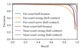
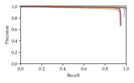
(a) Tennis (6 classes)

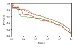
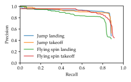
(b) FS-Comp (4 classes)

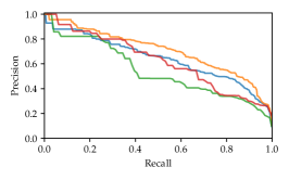
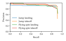
(c) FS-Perf (4 classes)

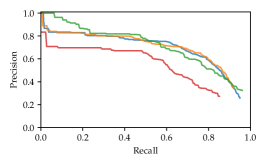
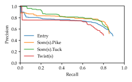
(d) FineDiving (4 classes)

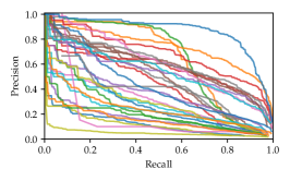
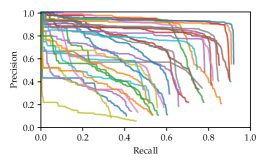
(e) FineGym-Full (32 classes)

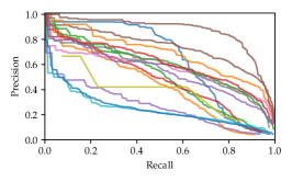
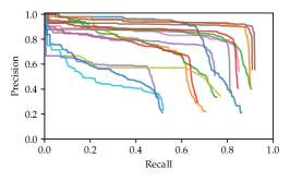
(f) FineGym-Start (16 classes)

Figure 3: Precision-recall curves for each event class at $\delta=1$, produced by E2E-Spot’s default configuration. Charts on the left are without NMS and charts on the right are with NMS. NMS improves precision by suppressing nearby detections but can also lead to lower recall.

Appendix 0.D Dataset Details

We use the Tennis [71], Figure Skating [27], FineDiving [65], and FineGym [47] datasets, with precise temporal event labels.

0.D.1 Tennis

The Tennis dataset is an extension of the dataset proposed by Zhang et al [71] to 19 new videos. Like the nine original videos from [71], the new videos are obtained from YouTube at full HD resolution and contain content from the US Open and Wimbledon tournaments. We annotate at least one full ‘set’ (a unit of gameplay) from each of the 19 new videos in order to diversify the dataset for training and evaluation.

To focus on the temporal aspect of precise spotting, we evaluate on the six top-level categories of events enumerated in § 4 and Table 10. These events are selected by their temporal definitions instead of the full set of semantic action attributes (e.g., swing type differentiated by topspin vs. slice; forehand vs. backhand; volley). The dataset contains 1.3M frames, of which 2.6% are precise temporal events.

0.D.2 Figure Skating

We extend the labels by Hong et al [27], which include fine-grained action classes and their temporal extents at approximately 1 second precision. To perform precise spotting, we manually re-annotate the labels to frame-accurate take-off and landing events.

As in Tennis, we separate temporally precise spotting from fine-grained classification of actions (e.g., the jump type) in order to focus on the temporal aspect of the spotting problem. See Table 11 for event statistics. The dataset contains 1.6M frames, of which only 0.23% are precise temporal events.

0.D.3 FineDiving

We use the pre-extracted frames provided by Xu et al [65] and spot the frames of transition between segments. The events include somersaults.pike, somersaults.tuck, twists, and entry. Note that we ignore the number of revolutions when generating frame-level event labels. See Table 12 for event statistics. The dataset contains 547K frames, of which 2.2% are precise temporal events.

0.D.4 FineGym

FineGym is a large gymnastics video dataset released by Shao et al [47]. It contains annotations for balance beam, floor exercises, uneven bars, and vaulting. The dataset is primarily used for action recognition, with 288 fine-grained classes and their time intervals. These actions are contained within individual performances (e.g., an untrimmed balance beam routine), and several performances appear in a single video from YouTube.

We detect precise events within the untrimmed performances and split the dataset three ways for training, validation, and testing; these splits do not contain overlap in performances and source videos. We discard any performances that do not contain temporal annotations, have malformed annotations, or have annotations that are missing a class label in Gym288, leaving 5,374 performances.

Shao et al. [47] propose a hierarchy of action categories (to which the Gym288 classes belong), and we reduce the spotting problem to the granularity of these categories (e.g., “balance beam dismounts” is one example). Because our focus is temporal precision, we leave the challenging task of (unbalanced) 288-way action classification, which can be performed after events have been spotted, to past and future work on fine-grained action recognition.

We define temporally precise events in FineGym as the start and end frames of action intervals. This definition is straightforward for actions in balance beam, floor exercises, and uneven bars. Each vault, however, is specified as a sequence of three back-to-back segments, which we convert into four events. See Table 13 for the event breakdown and statistics.

A minority of videos (259) in the FineGym dataset have frame rates higher than 25–30 FPS. For consistency, since our spotting tolerances are defined in $\delta$ frames, we resample those videos to between 25–30 FPS. The final dataset contains 7.6M frames, 1.1% of which are precise temporal events.

Table 10: Tennis dataset: event classes and their counts.

Event class	Train	Val	Test
Near-court serve (ball contact)	673	238	779
Near-court swing (ball contact)	2199	709	4136
Near-court ball bounce	2606	871	4650
Far-court serve (ball contact)	657	200	800
Far-court swing (ball contact)	2220	757	4146
Far-court ball bounce	2621	867	4662

Table 11: Figure Skating dataset: event classes and their counts.

	FS-Comp			FS-Perf
Event class	Train	Val	Test	Train	Val	Test
Jump takeoff	704	233	527	723	372	369
Jump landing	704	233	527	723	372	369
Flying spin takeoff	178	59	136	183	94	96
Flying spin landing	178	59	136	183	94	96

Table 12: FineDiving dataset: event classes and their counts.

Event class	Train	Val	Test
Entry	1794	449	741
Som(s).Pike	1254	345	553
Som(s).Tuck	667	149	255
Twist(s)	467	120	216

Table 13: FineGym dataset: event classes and their counts. The classes are based on the ‘set-level categories’ defined by Shao et al [47]. We refer to the full set of classes as FineGym-Full and a more visually consistent subset, containing primarily start events, as FineGym-Start.

Event class	In FineGym-Start	Train	Val	Test
Floor exercise leap_jump_hop start		2007	602	629
Floor exercise leap_jump_hop end		2007	602	629
Floor exercise turns start		683	197	223
Floor exercise turns end		683	197	223
Floor exercise side_salto start		23	13	13
Floor exercise side_salto end		23	13	13
Floor exercise front_salto start		818	259	268
Floor exercise front_salto end		818	259	268
Floor exercise back_salto start		1850	524	604
Floor exercise back_salto end		1850	524	604
Balance beam leap_jump_hop start		3062	765	960
Balance beam leap_jump_hop end		3062	765	960
Balance beam turns start		857	215	299
Balance beam turns end		857	215	299
Balance beam flight_salto start		2637	720	830
Balance beam flight_salto end		2637	720	830
Balance beam flight_handspring start		1835	440	618
Balance beam flight_handspring end		1835	440	618
Balance beam dismounts start		763	188	267
Balance beam dismounts end		763	188	267
Uneven bars circles start		4143	1151	1318
Uneven bars circles end		4143	1151	1318
Uneven bars flight_same_bar start		1029	270	325
Uneven bars flight_same_bar end		1029	270	325
Uneven bars transition_flight start		2079	630	680
Uneven bars transition_flight end		2079	630	680
Uneven bars dismounts start		750	225	252
Uneven bars dismounts end		750	225	252
Vault (timestamp 0)		1263	367	401
Vault (timestamp 1)		1263	367	401
Vault (timestamp 2)		1263	367	401
Vault (timestamp 3)		1263	367	401

References

- [1] Ahn, H., Lee, D.: Refining action segmentation with hierarchical video representations. In: Proceedings of the IEEE/CVF International Conference on Computer Vision (ICCV). pp. 16302–16310 (October 2021)
- [2] Alwassel, H., Giancola, S., Ghanem, B.: TSP: Temporally-sensitive pretraining of video encoders for localization tasks. In: Proceedings of the IEEE/CVF International Conference on Computer Vision (ICCV) Workshops. pp. 3173–3183 (October 2021)
- [3] Buch, S., Escorcia, V., Ghanem, B., Niebles, J.C.: End-to-end, single-stream temporal action detection in untrimmed videos. In: Proceedings of the British Machine Vision Conference (BMVC) (September 2017)
- [4] Buch, S., Escorcia, V., Shen, C., Ghanem, B., Carlos Niebles, J.: SST: Single-stream temporal action proposals. In: Proceedings of the IEEE Conference on Computer Vision and Pattern Recognition (CVPR) (July 2017)
- [5] Caba Heilbron, F., Escorcia, V., Ghanem, B., Carlos Niebles, J.: ActivityNet: A large-scale video benchmark for human activity understanding. In: Proceedings of the IEEE Conference on Computer Vision and Pattern Recognition (CVPR) (June 2015)
- [6] Carreira, J., Zisserman, A.: Quo vadis, action recognition? A new model and the Kinetics dataset. In: Proceedings of the IEEE Conference on Computer Vision and Pattern Recognition (CVPR) (July 2017)
- [7] Chen, M.H., Li, B., Bao, Y., AlRegib, G.: Action segmentation with mixed temporal domain adaptation. In: Proceedings of the IEEE/CVF Winter Conference on Applications of Computer Vision (WACV) (March 2020)
- [8] Chung, J., Gulcehre, C., Cho, K., Bengio, Y.: Empirical evaluation of gated recurrent neural networks on sequence modeling. In: Proceedings of NIPS Deep Learning and Representation Learning Workshop (2014)
- [9] Cioppa, A., Deliege, A., Giancola, S., Ghanem, B., Van Droogenbroeck, M., Gade, R., Moeslund, T.B.: A context-aware loss function for action spotting in soccer videos. In: IEEE/CVF Conference on Computer Vision and Pattern Recognition (CVPR) (June 2020)
- [10] Dai, R., Das, S., Minciullo, L., Garattoni, L., Francesca, G., Bremond, F.: PDAN: Pyramid dilated attention network for action detection. In: Proceedings of the IEEE/CVF Winter Conference on Applications of Computer Vision (WACV). pp. 2970–2979 (January 2021)
- [11] Dai, R., Das, S., Sharma, S., Minciullo, L., Garattoni, L., Bremond, F., Francesca, G.: Toyota Smarthome Untrimmed: Real-world untrimmed videos for activity detection (2020), arXiv:2010.14982
- [12] Damen, D., Doughty, H., Farinella, G.M., Fidler, S., Furnari, A., Kazakos, E., Moltisanti, D., Munro, J., Perrett, T., Price, W., Wray, M.: Scaling egocentric vision: The EPIC-KITCHENS dataset. In: Proceedings of the European Conference on Computer Vision (ECCV) (September 2018)
- [13] Deliege, A., Cioppa, A., Giancola, S., Seikavandi, M.J., Dueholm, J.V., Nasrollahi, K., Ghanem, B., Moeslund, T.B., Van Droogenbroeck, M.: SoccerNet-v2: A dataset and benchmarks for holistic understanding of broadcast soccer videos. In: Proceedings of the IEEE/CVF Conference on Computer Vision and Pattern Recognition (CVPR) Workshops. pp. 4508–4519 (June 2021)
- [14] Deliège, A., Cioppa, A., Giancola, S., Seikavandi, M.J., Dueholm, J.V., Nasrollahi, K., Ghanem, B., Moeslund, T.B., Droogenbroeck, M.V.: SoccerNet - action spotting. https://github.com/SoccerNet/sn-spotting (2022)
- [15] Deng, J., Dong, W., Socher, R., Li, L.J., Li, K., Fei-Fei, L.: ImageNet: A large-scale hierarchical image database. In: Proceedings of the IEEE/CVF Conference on Computer Vision and Pattern Recognition (CVPR) (June 2009)
- [16] Ding, L., Xu, C.: TricorNet: A hybrid temporal convolutional and recurrent network for video action segmentation (2017), arXiv:1705.07818
- [17] Dosovitskiy, A., Beyer, L., Kolesnikov, A., Weissenborn, D., Zhai, X., Unterthiner, T., Dehghani, M., Minderer, M., Heigold, G., Gelly, S., Uszkoreit, J., Houlsby, N.: An image is worth 16x16 words: Transformers for image recognition at scale. In: International Conference on Learning Representations (ICLR) (2021)
- [18] Fan, H., Murrell, T., Wang, H., Alwala, K.V., Li, Y., Li, Y., Xiong, B., Ravi, N., Li, M., Yang, H., Malik, J., Girshick, R., Feiszli, M., Adcock, A., Lo, W.Y., Feichtenhofer, C.: PyTorchVideo: A deep learning library for video understanding. In: Proceedings of the 29th ACM International Conference on Multimedia (2021)
- [19] Fan, H., Xiong, B., Mangalam, K., Li, Y., Yan, Z., Malik, J., Feichtenhofer, C.: Multiscale vision transformers. In: Proceedings of the IEEE/CVF International Conference on Computer Vision (ICCV). pp. 6824–6835 (October 2021)
- [20] Farha, Y.A., Gall, J.: MS-TCN: Multi-stage temporal convolutional network for action segmentation. In: Proceedings of the IEEE/CVF Conference on Computer Vision and Pattern Recognition (CVPR) (June 2019)
- [21] Fathi, A., Ren, X., Rehg, J.M.: Learning to recognize objects in egocentric activities. In: Proceedings of the IEEE/CVF Conference on Computer Vision and Pattern Recognition (CVPR) (June 2011)
- [22] Feichtenhofer, C., Fan, H., Malik, J., He, K.: SlowFast networks for video recognition. In: Proceedings of the IEEE/CVF International Conference on Computer Vision (ICCV) (October 2019)
- [23] Giancola, S., Ghanem, B.: Temporally-aware feature pooling for action spotting in soccer broadcasts. In: Proceedings of the IEEE/CVF Conference on Computer Vision and Pattern Recognition (CVPR) Workshops. pp. 4490–4499 (June 2021)
- [24] Girshick, R., Donahue, J., Darrell, T., Malik, J.: Rich feature hierarchies for accurate object detection and semantic segmentation. In: Proceedings of the IEEE Conference on Computer Vision and Pattern Recognition (CVPR) (June 2014)
- [25] Hao, Y., Zhang, H., Ngo, C.W., Liu, Q., Hu, X.: Compact bilinear augmented query structured attention for sport highlights classification. In: Proceedings of the 28th ACM International Conference on Multimedia. pp. 628–636. Association for Computing Machinery, New York, NY, USA (2020)
- [26] He, K., Zhang, X., Ren, S., Sun, J.: Deep residual learning for image recognition. In: Proceedings of the IEEE Conference on Computer Vision and Pattern Recognition (CVPR) (June 2016)
- [27] Hong, J., Fisher, M., Gharbi, M., Fatahalian, K.: Video pose distillation for few-shot, fine-grained sports action recognition. In: Proceedings of the IEEE/CVF International Conference on Computer Vision (ICCV). pp. 9254–9263 (October 2021)
- [28] Ibrahim, M.S., Muralidharan, S., Deng, Z., Vahdat, A., Mori, G.: A hierarchical deep temporal model for group activity recognition. In: Proceedings of the IEEE Conference on Computer Vision and Pattern Recognition (CVPR) (June 2016)
- [29] Ishikawa, Y., Kasai, S., Aoki, Y., Kataoka, H.: Alleviating over-segmentation errors by detecting action boundaries. In: Proceedings of the IEEE/CVF Winter Conference on Applications of Computer Vision (WACV). pp. 2322–2331 (January 2021)
- [30] Jiang, Y.G., Liu, J., Roshan Zamir, A., Toderici, G., Laptev, I., Shah, M., Sukthankar, R.: THUMOS Challenge: Action recognition with a large number of classes (2014)
- [31] Kay, W., Carreira, J., Simonyan, K., Zhang, B., Hillier, C., Vijayanarasimhan, S., Viola, F., Green, T., Back, T., Natsev, P., Suleyman, M., Zisserman, A.: The Kinetics human action video dataset (2017), arXiv:1705.06950
- [32] Kuehne, H., Arslan, A., Serre, T.: The language of actions: Recovering the syntax and semantics of goal-directed human activities. In: Proceedings of the IEEE Conference on Computer Vision and Pattern Recognition (CVPR) (June 2014)
- [33] Li, A., Thotakuri, M., Ross, D.A., Carreira, J., Vostrikov, A., Zisserman, A.: The AVA-Kinetics localized human actions video dataset (2020), arXiv:2005.00214
- [34] Li, Y., Li, Y., Vasconcelos, N.: RESOUND: Towards action recognition without representation bias. In: Proceedings of the European Conference on Computer Vision (ECCV) (September 2018)
- [35] Li, Y., Chen, L., He, R., Wang, Z., Wu, G., Wang, L.: MultiSports: A multi-person video dataset of spatio-temporally localized sports actions. In: Proceedings of the IEEE/CVF International Conference on Computer Vision (ICCV). pp. 13536–13545 (October 2021)
- [36] Lin, C., Xu, C., Luo, D., Wang, Y., Tai, Y., Wang, C., Li, J., Huang, F., Fu, Y.: Learning salient boundary feature for anchor-free temporal action localization. In: Proceedings of the IEEE/CVF Conference on Computer Vision and Pattern Recognition (CVPR). pp. 3320–3329 (June 2021)
- [37] Lin, J., Gan, C., Han, S.: TSM: Temporal shift module for efficient video understanding. In: Proceedings of the IEEE/CVF International Conference on Computer Vision (ICCV) (October 2019)
- [38] Lin, T., Liu, X., Li, X., Ding, E., Wen, S.: BMN: Boundary-matching network for temporal action proposal generation. In: Proceedings of the IEEE/CVF International Conference on Computer Vision (ICCV) (October 2019)
- [39] Lin, T., Zhao, X., Su, H., Wang, C., Yang, M.: BSN: Boundary sensitive network for temporal action proposal generation. In: Proceedings of the European Conference on Computer Vision (ECCV) (September 2018)
- [40] Liu, X., Bai, S., Bai, X.: An empirical study of end-to-end temporal action detection. In: Proceedings of the IEEE/CVF Conference on Computer Vision and Pattern Recognition (CVPR). pp. 20010–20019 (June 2022)
- [41] Liu, X., Hu, Y., Bai, S., Ding, F., Bai, X., Torr, P.H.S.: Multi-shot temporal event localization: A benchmark. In: Proceedings of the IEEE/CVF Conference on Computer Vision and Pattern Recognition (CVPR). pp. 12596–12606 (June 2021)
- [42] Loshchilov, I., Hutter, F.: SGDR: Stochastic gradient descent with warm restarts. In: Proceedings of the International Conference on Learning Representations (ICLR) (2017)
- [43] Loshchilov, I., Hutter, F.: Decoupled weight decay regularization. In: Proceedings of the International Conference on Learning Representations (ICLR) (2019)
- [44] Nvidia: Nvidia RTX A5000 data sheet (2021)
- [45] PyTorch: Pytorch documentation: Transformer (2022)
- [46] Radosavovic, I., Kosaraju, R.P., Girshick, R., He, K., Dollar, P.: Designing network design spaces. In: Proceedings of the IEEE/CVF Conference on Computer Vision and Pattern Recognition (CVPR) (June 2020)
- [47] Shao, D., Zhao, Y., Dai, B., Lin, D.: FineGym: A hierarchical video dataset for fine-grained action understanding. In: Proceedings of the IEEE/CVF Conference on Computer Vision and Pattern Recognition (CVPR) (June 2020)
- [48] Sigurdsson, G., Choi, J.: Charades Challenge (2017)
- [49] Sigurdsson, G.A., Divvala, S., Farhadi, A., Gupta, A.: Asynchronous temporal fields for action recognition. In: Proceedings of the IEEE Conference on Computer Vision and Pattern Recognition (CVPR) (July 2017)
- [50] Sigurdsson, G.A., Varol, G., Wang, X., Farhadi, A., Laptev, I., Gupta, A.: Hollywood in homes: Crowdsourcing data collection for activity understanding. In: Proceedings of the European Conference on Computer Vision (ECCV) (September 2016)
- [51] Singh, B., Marks, T.K., Jones, M., Tuzel, O., Shao, M.: A multi-stream bi-directional recurrent neural network for fine-grained action detection. In: Proceedings of the IEEE Conference on Computer Vision and Pattern Recognition (CVPR) (June 2016)
- [52] Singh, B., Marks, T.K., Jones, M., Tuzel, O., Shao, M.: A multi-stream bi-directional recurrent neural network for fine-grained action detection. In: Proceedings of the IEEE Conference on Computer Vision and Pattern Recognition (CVPR) (June 2016)
- [53] Singhania, D., Rahaman, R., Yao, A.: Coarse to fine multi-resolution temporal convolutional network (2021), arXiv:2105.10859
- [54] Soares, J.V.B., Shah, A.: Action spotting using dense detection anchors revisited: Submission to the SoccerNet Challenge 2022 (2022), arXiv:2206.07846
- [55] Soares, J.V.B., Shah, A., Biswas, T.: Temporally precise action spotting in soccer videos using dense detection anchors (2022), arXiv:2205.10450
- [56] Stein, S., McKenna, S.J.: Combining embedded accelerometers with computer vision for recognizing food preparation activities. In: Proceedings of ACM International Joint Conference on Pervasive and Ubiquitous Computing (UbiComp). pp. 729–738. Association for Computing Machinery, New York, NY, USA (2013)
- [57] Sudhakaran, S., Escalera, S., Lanz, O.: Gate-shift networks for video action recognition. In: Proceedings of the IEEE/CVF Conference on Computer Vision and Pattern Recognition (CVPR) (June 2020)
- [58] Teed, Z., Deng, J.: RAFT: Recurrent all-pairs field transforms for optical flow. In: Proceedings of the European Conference on Computer Vision (ECCV) (August 2020)
- [59] Tirupattur, P., Duarte, K., Rawat, Y.S., Shah, M.: Modeling multi-label action dependencies for temporal action localization. In: Proceedings of the IEEE/CVF Conference on Computer Vision and Pattern Recognition (CVPR). pp. 1460–1470 (June 2021)
- [60] Tomei, M., Baraldi, L., Calderara, S., Bronzin, S., Cucchiara, R.: RMS-Net: Regression and masking for soccer event spotting. In: 2020 25th International Conference on Pattern Recognition (ICPR). pp. 7699–7706. IEEE Computer Society, Los Alamitos, CA, USA (Jan 2021)
- [61] Tran, D., Wang, H., Torresani, L., Ray, J., LeCun, Y., Paluri, M.: A closer look at spatiotemporal convolutions for action recognition. In: Proceedings of the IEEE Conference on Computer Vision and Pattern Recognition (CVPR) (June 2018)
- [62] TwentyBN: The 20BN-something-something dataset v2
- [63] Wang, L., Xiong, Y., Wang, Z., Qiao, Y., Lin, D., Tang, X., Val Gool, L.: Temporal segment networks: Towards good practices for deep action recognition. In: Proceedings of the European Conference on Computer Vision (ECCV) (September 2016)
- [64] Wightman, R.: PyTorch image models. https://github.com/rwightman/pytorch-image-models (2019)
- [65] Xu, J., Rao, Y., Yu, X., Chen, G., Zhou, J., Lu, J.: FineDiving: A fine-grained dataset for procedure-aware action quality assessment. In: Proceedings of the IEEE/CVF Conference on Computer Vision and Pattern Recognition (CVPR). pp. 2949–2958 (June 2022)
- [66] Xu, M., Zhao, C., Rojas, D.S., Thabet, A., Ghanem, B.: G-TAD: Sub-graph localization for temporal action detection. In: Proceedings of the IEEE/CVF Conference on Computer Vision and Pattern Recognition (CVPR) (June 2020)
- [67] Yeung, S., Russakovsky, O., Jin, N., Andriluka, M., Mori, G., Fei-Fei, L.: Every moment counts: Dense detailed labeling of actions in complex videos. International Journal of Computer Vision 126(2-4), 375–389 (2018)
- [68] Yi, F., Wen, H., Jiang, T.: ASFormer: Transformer for action segmentation. In: Proceedings of the British Machine Vision Conference (BMVC) (November 2021)
- [69] Zeng, R., Huang, W., Tan, M., Rong, Y., Zhao, P., Huang, J., Gan, C.: Graph convolutional networks for temporal action localization. In: Proceedings of the IEEE/CVF International Conference on Computer Vision (ICCV) (October 2019)
- [70] Zhang, C., Wu, J., Li, Y.: ActionFormer: Localizing moments of actions with transformers (2022), arXiv:2202.07925
- [71] Zhang, H., Sciutto, C., Agrawala, M., Fatahalian, K.: Vid2Player: Controllable video sprites that behave and appear like professional tennis players. ACM Transactions on Graphics 40(3) (2021)
- [72] Zhang, H., Cisse, M., Dauphin, Y.N., Lopez-Paz, D.: mixup: Beyond empirical risk minimization. In: Proceedings of the International Conference on Learning Representations (ICLR) (2018)
- [73] Zhao, C., Thabet, A.K., Ghanem, B.: Video self-stitching graph network for temporal action localization. In: Proceedings of the IEEE/CVF International Conference on Computer Vision (ICCV). pp. 13658–13667 (October 2021)
- [74] Zhou, B., Andonian, A., Oliva, A., Torralba, A.: Temporal relational reasoning in videos. In: Proceedings of the European Conference on Computer Vision (ECCV) (September 2018)
- [75] Zhou, X., Kang, L., Cheng, Z., He, B., Xin, J.: Feature combination meets attention: Baidu soccer embeddings and transformer based temporal detection (2021), arXiv:2106.14447