Extremal inhomogeneous Gibbs states
for SOS-models and finite-spin models on trees

Abstract.

We consider ${\mathbb{Z}}$-valued $p$-SOS-models with nearest neighbor interactions of the form $|\omega_{v}-\omega_{w}|^{p}$, and finite-spin ferromagnetic models on regular trees. This includes the classical SOS-model, the discrete Gaussian model and the Potts model.

We exhibit a family of extremal inhomogeneous (i.e. tree automorphism non-invariant) Gibbs measures arising as low temperature perturbations of ground states (local energy minimizers), which have a sparse enough set of broken bonds together with uniformly bounded increments along them. These low temperature states in general do not possess any symmetries of the tree.

This generalises the results of Gandolfo, Ruiz and Shlosman [27] about the Ising model, and shows that the latter behaviour is robust. We treat three different types of extensions: non-compact state space gradient models, models without spin-symmetry, and models in small random fields.

We give a detailed construction and full proofs of the extremality of the low-temperature states in the set of all Gibbs measures, analysing excess energies relative to the ground states, convergence of low-temperature expansions, and properties of cutsets.

1. Introduction

Amongst probability measures on lattice spin systems, Gibbs states on trees have special properties, widely studied for almost fifty years by now, see e.g. [45, 40, 47, 33, 32, 39].

In the early nineties, Blekher and Ganikhodgaev [9], following a strategy already proposed by Higuchi in the late seventies [33], show that the Ising model (in zero external field, on regular trees) possesses uncountably many interface states, which are extremal and non translation invariant, as soon as $T<T_{c}$. In 2008, Rozikov and Rakhmatullaev [42] exhibit non-translation invariant measures corresponding to subgroups in the group representation of the Cayley tree, the so-called "weakly periodic" Gibbs measures. These states can be thought of generalizations of Dobrushin states from [19, 5], but with many interfaces, possibly countably infinitely many.

In 2012, Gandolfo, Ruiz and Shlosman [27], exhibit a rich family of extremal inhomogeneous (i.e. tree automorphism non-invariant) Gibbs measures arising as low temperature perturbations of ground states (local energy minimizers), which have a sparse enough set of broken bonds, see also [28]. These low temperature states in general do not possess any symmetries of the tree.

The aim of the present paper is to show that the latter behaviour is robust. We prove it to hold in three different types of extensions of the Ising model:

• non-compact state space gradient models

• models without spin-symmetry

• models in small random fields

The main objective is to study integer-valued gradient models, but we also derive similar results for general finite-alphabet spin models of ferromagnetic type, including the Potts model.

Gradient models belong to a very active field of research, also widely studied in the literature, either on lattices to model effective interfaces, see e.g. [13, 24, 18, 44, 6, 21, 7, 37, 16, 17, 38] or more specifically on trees [31, 29, 30, 43].

In [29], Henning and Kuelske prove, for very general classes of gradient interactions, assuming strong enough coupling, that there exist homogeneous Gibbs states which are strongly localised around one given height. The method of proof is analytic in character and based on finding fixed points of a suitable non-linear operator in a $l^{p}({\mathbb{Z}})$-sequence space of so-called boundary laws, starting from the description of Zachary [47], see also [4, 20]. Strong coupling of the interactions allows to prove that the relevant operator is a contraction. A variant of that contraction method is used to prove the existence of a different type of consistent measures, namely delocalized gradient Gibbs measures (with unbounded height-fluctuations), still in strong coupling regimes. Interestingly, coexistence of delocalized and localized states for the same interaction parameters is possible. Using dynamical systems ideas with an analysis of the unstable manifold around the free state, special types of inhomogenous gradient states are constructed, which still possess some rotation invariance, see [30].

The present work first treats general $p$-SOS models, with nearest neighbor interactions, where the interaction along an edge $(v,w)$ of the tree is of the form $\beta|\omega_{v}-\omega_{w}|^{p}$, with a fixed interaction exponent $p\in(0,\infty)$, and sufficiently large inverse temperature $\beta\in(0,\infty)$. The cases $p=1$ (the classical SOS-model) and $p=2$ (discrete Gaussian, DGFF) are the most popular choices, see e.g. [46, 2, 3] and references therein. Our approach to inhomogeneous states is completely independent from the latter two results [29, 30], based on the boundary law formalism. Instead of it, we rigorously develop low-temperature expansions around a suitable class of ground states generalising the ones initially introduced in [27] in the case of the Ising model. These ground states do not possess any symmetries as rotation invariance in general.

More precisely, in this enlarged framework, we generalise the definition of contours (or low temperature excitations), including increment sizes (which were not needed for Ising) and give a new proof of the control on the excess energy created by a low temperature excitation above a given non-homogeneous configuration. When this configuration has a sparse set of broken bonds, together with bounded increments, the excess energy control allows to conclude that it is a stable local ground state provided the degree of the tree is large enough. We provide rigorous proofs of :

• tightness and convergence of finite volume measures with boundary conditions given by these non-hommogenous configurations

• extremality of the low temperature states, derived from cluster expansion and cutset properties.

• the stability of the excess-energy control under the addition of small local field terms, which provides the extension of our results to models in small random fields.

Note that our contours have empty interior, a tree-specific property which provides more control in Peierls-type estimates and low-temperature expansions, also around inhomogeneous ground states. This allows to prove more refined results than on the lattice, where versions of Pirogov-Sinai theory would be necessary to treat situations without symmetry in spin space, even when there is spatial homogeneity, see e.g. Chapter 7 of [25]. This particularity allows us to prove the stability of these inhomogeneous ground states, and existence of well-defined infinite volume limits with the required decorrelation properties, by combining statistical mechanics technics (as cluster expansions) with probabilistic methods (cutsets, Fourier transforms, etc.).

The paper is organised as follows. In Section 2, we state our results on the stability of some ground states at low temperature. We first treat general $p$-SOS models (Theorem 1), and afterwards come to general finite-alphabet models, including the Potts model (Theorem 2).

In Section 3 we provide the definition of contours, as well as the proof of their excess energy estimate (Lemma 1).

In Section 4, we consider these contours as polymers to perform cluster expansions within the framework of Bovier-Zahradník [14] and study the low-temperature states. We use the estimates they provide in addition to the convergence of the expansions to prove Theorem 1 and Theorem 2. We get an exponential control of the polymer weights (Proposition 3), convergence of finite-dimensional marginals via Fourier transforms (Lemma LABEL:Lem3), quantitative tightness in the unbounded spins case (Section LABEL:sec-tightness), DLR-property of the limiting measures (Section LABEL:sec-DLR), identifiability of the different low-temperatures phases obtained from sparse ground states (Section LABEL:sec-DLR). Finally, in Section LABEL:sec-cutset, we derive cutset properties as well as correlation decay for events of polymer type, that eventually lead to extremality.

In Section 5 we describe applications of our theory to existence of extremal states for inhomogeneous locally perturbed models. This includes the random field Potts model, and the $p$-SOS model in random fields and in random media.

2. Definitions and main results

Let $\mathcal{T}^{d}=(V,E)$ denote the Cayley tree of order $d$, on which any vertex $i\in V$ has exactly $d+1$ neighbors. To any vertex $i\in V$, we attach a spin, which is a random variable $\sigma_{i}$ taking values in $\Omega_{0}$. The spin space $\Omega_{0}$ we consider will be either the discrete set ${\mathbb{Z}}_{q}=\{0,\dots,q-1\}$, for $q\in\{2,3,\ldots\}$, or the unbounded countable set ${\mathbb{Z}}$, equipped with a product $\sigma$-algebra $\mathcal{E}=\mathcal{P}(\Omega_{0})$. We are interested in probability measures on the product space $(\Omega,\mathcal{F})=(\Omega_{0}^{V},\mathcal{E}^{\otimes V})$. For any subset $\Lambda\subset V$ we define $\omega_{\Lambda}=(\omega_{v})_{v\in\Lambda}$. For any subset $W\subset V$ we denote by $\mathcal{F}_{W}$ the sigma algebra generated by the variables $(\sigma_{i})_{i\in W}$. If $\Lambda\subset V$ is a finite subset, we write $\Lambda\Subset V$.

We introduce an interaction potential $\Phi$ and consider equilibrium states to be Gibbs measures built with the DLR framework, see e.g. [32]: they are the probability measures $\mu$ consistent with the Gibbsian specification $\gamma^{\Phi}$ in the sense that a version of their conditional probabilities w.r.t. the outside of any finite set $\Lambda$ of the tree is given by the corresponding element of the Gibbs specification $\gamma_{\Lambda}^{\Phi}$, that is

$$\forall\Lambda\Subset V,\;\forall\omega_{\Lambda}\in\Omega_{\Lambda},\;\mu[\sigma_{\Lambda}=\omega_{\Lambda}\mid\mathcal{F}_{\Lambda^{c}}](\cdot)=\gamma_{\Lambda}^{\Phi}(\omega_{\Lambda}\mid\cdot),\;\mu-a.s.$$

where the elements of the Gibbs specification $\gamma^{\Phi}=\gamma^{\Phi}(\beta)$ are the probability kernels $\gamma_{\Lambda}^{\Phi}$ from $\Omega_{\Lambda^{c}}$ to $\mathcal{F}_{\Lambda}$ defined for all finite $\Lambda$ as

$$\gamma_{\Lambda}^{\Phi}(\omega_{\Lambda}\mid\tau_{\Lambda^{c}})=\frac{1}{Z_{\Lambda}^{\tau}}e^{-\beta H_{\Lambda}(\omega_{\Lambda}\tau_{\Lambda^{c}})}.$$

The partition function $Z_{\Lambda}^{\tau}$ is the usual normalization constant for a fixed boundary condition $\tau$, at finite volume $\Lambda$, and the Hamiltonian $H_{\Lambda}^{\Phi}$ with boundary condition $\tau$ is there provided by $H_{\Lambda}(\omega_{\Lambda}\tau_{\Lambda^{c}})=\sum_{A\cap\Lambda\neq\emptyset}\Phi_{A}(\omega_{\Lambda}\tau_{\Lambda^{c}})$ where $\omega_{\Lambda}\tau_{\Lambda^{c}}$ denotes the concatenation of $\omega_{\Lambda}$ and $\tau_{\Lambda^{c}}$. We sometimes shortly write $H$ for the Hamiltonian with free boundary conditions:

$$H(\omega)=H_{\Lambda}^{f}(\omega):=\sum_{A\subset\Lambda}\Phi_{A}(\omega_{\Lambda}).$$ (2.1)

The ferromagnetic potentials we consider are nearest-neighbor potentials and will be generically denoted by $\Phi$. Pairs $\{i,j\}\in E$ of nearest-neighbors are written $i\sim j$. In the case where $\Omega_{0}$ is unbounded, we consider $p$-SOS models, where the potential is given for any $p>0$ by

$$\Phi_{ij}(\omega)=|\omega_{i}-\omega_{j}|^{p}\quad\text{for all}\quad i\sim j$$ (2.2)

and 0 otherwise, where $\mid\cdot\mid$ is the absolute value. In the case where $\Omega_{0}={\mathbb{Z}}_{q}$, we consider any nearest neighbor model of the form

$$\Phi_{ij}(\omega)=\sum_{k,\ell=0}^{q-1}u_{k,\ell}\mathbf{1}_{\omega_{i}=k,\omega_{j}=\ell}\text{ where }{\forall k,\ell\in{\mathbb{Z}}_{q},u_{k,\ell}\geq 0}\text{ and }u_{k,k}=0.$$ (2.3)

The latter includes the $q$-state Potts model, for which

$$\Phi_{ij}(\omega)=\mathbf{1}_{\omega_{i}\neq\omega_{j}}.$$ (2.4)

For a given set of edges $D\subset E$, and a given vertex $v\in V$ we define $d_{D}(v)$ to be the number of bonds in $D$ which are incident to $v$. Then, we define the number :

$$d_{D}=\max_{v\in V}d_{D}(v).$$

2.1. p-SOS models

Existence of phase transitions on trees with homogeneous phases holds for very general interactions at low-temperature [29, 30]. However, we investigate here the low-temperature stability of non translation-invariant (inhomogeneous) ground states, defined as follows below (see an example in Figure 1), and show how they are related to infinite-volume Gibbs measures. Our first main result reads then:

Theorem 1.

Let $p>0$ and consider the $p$-SOS models (2.2) on the Cayley tree of degree $d$. Let $d_{\max},M\in{\mathbb{N}}_{0}$, where $d_{\max}\leq d$. Define ${\mathcal{G}}^{0}={\mathcal{G}}^{0}({d_{\max}},{d},M)$ to be the set of configurations $\omega^{0}\in{\mathbb{Z}}^{V}$ which satisfy the following sparsity requirement on the set of broken edges and have uniformly bounded spin increments along them:

1. The set of broken edges $D:=\{\{v,w\}\in E:\omega^{0}_{v}\neq\omega^{0}_{w}\}$ is such that $d_{D}\leq d_{\max}$.

2. All increments are uniformly bounded by $M$: $\max_{v\sim w}|\omega^{0}_{v}-\omega^{0}_{w}|\leq M$.

Then, for each interaction exponent $p>0$, each maximal increment size $M\in{\mathbb{N}}_{0}$, and each maximal internal degree $d_{\max}\in{\mathbb{N}}_{0}$ there is a minimal degree $d(p,M,{d_{\max}})$ such that for all degrees $d\geq d(p,M,{d_{\max}})$ the following holds:

There exists a finite $\beta_{0}=\beta_{0}(d,p,{d_{\max}},M)$ such that for all $\beta\geq\beta_{0}$ for the $p$-SOS model on the regular tree of degree $d$, there is a family of Gibbs measures $(\mu^{\omega^{0}}_{\beta})_{\omega^{0}\in{\mathcal{G}}^{0}}$ with the properties

1. $\omega^{0}\neq\tau^{0}$ implies $\mu^{\omega^{0}}_{\beta}\neq\mu^{\tau^{0}}_{\beta}$.

2. The measures $\mu^{\omega^{0}}_{\beta}$ are extremal in the set of all Gibbs measures.

3. $\mu^{\omega^{0}}_{\beta}$ concentrates around $\omega^{0}$ in the sense that there exist two positive constants $c,C$ such that for any $v\in V$ and for all increments $k\in{\mathbb{Z}}$,

   $$\begin{split}&\mu^{\omega^{0}}_{\beta}(\sigma_{v}-\omega_{v}^{0}=k)\leq Ce^{-c\beta|k|^{p}}.\end{split}$$ (2.5)

Remark. Further properties will be derived in the explicit construction, see below. Moreover, the assumptions 1 and 2 of Theorem 1 can be replaced by the more general assumption (LABEL:generalsparsity) below which mixes geometric sparsity and boundedness of heights.

2.2. Finite-spin ferromagnetic models

We have an analogous theorem in the situation of finite-alphabet models (2.3) with generalized ferromagnetic interactions $\Phi\geq 0$ in the following sense.

Theorem 2.

Let $q\in{\mathbb{N}}_{0}$ and consider the $q$-spin model (2.3) on the Cayley tree of degree $d$. Let $d_{\max}\in{\mathbb{N}}_{0}$, with $d_{\max}\leq d$. Put $u:={\min}_{k\neq\ell}u_{k,\ell}$ and $U:=\max_{k,\ell}u_{k,\ell}$. Define ${\mathcal{G}}_{q}^{0}={\mathcal{G}}_{q}^{0}({d_{\max},{d}})$ to be the set of configurations $\omega^{0}\in{\mathbb{Z}}^{V}$ whose set of broken bonds $D=\{\{v,w\}\in E:\omega^{0}_{v}\neq\omega^{0}_{w}\}$ is such that $d_{D}\leq d_{\max}$.

Then, under the following geometric sparsity condition on the set of broken bonds

$$(d-1)u>d_{\max}(U+u)$$ (2.6)

there exists a finite $\beta_{0}=\beta_{0}(d,q,u,U,{d_{\max}})\;{>0}$ such that for all $\beta\geq\beta_{0}$ there is a family of Gibbs measures $(\mu^{\omega^{0}}_{\beta})_{\omega^{0}\in{\mathcal{G}}^{0}}$ with the following properties:

1. $\omega^{0}\neq\tau^{0}$ implies $\mu^{\omega^{0}}_{\beta}\neq\mu^{\tau^{0}}_{\beta}$.

2. The measures $\mu^{\omega^{0}}_{\beta}$ are extremal in the set of all Gibbs measures.

3. $\mu^{\omega^{0}}_{\beta}$ concentrates around $\omega^{0}$ in the sense that there exist two positive constants $c,C$ such that for any vertex $v\in V$,

   $$\begin{split}&\mu^{\omega^{0}}_{\beta}(\sigma_{v}=\omega_{v}^{0})\geq 1-Ce^{-c\beta}.\end{split}$$ (2.7)

Remark: In the case of the Potts model (2.4), we have $u=U=1$ and thus the sparsity assumption (2.6) on $d_{\max}$ becomes $2d_{\max}<d-1$ which coincides with the sparsity requirement for the Ising model given in [27]. See Figure 1 for an example.

3. Excess energy for sparse ground states

In this section, we derive useful lower bounds on excess energies in our models, which are the starting point of the low-temperature expansions and extensions. Similar estimates were obtained for the Ising model in [27] using induction over the size of the contours. Here we follow a different non-inductive approach which provides useful bounds in the case of unbounded spins.

Let us start with the introduction of contours as labelled contours, namely as pairs of supports $\gamma$ and spin configurations $\omega_{\gamma}$ on these supports.

Definition 1.

Let $\omega^{0}\in\Omega_{0}^{V}$ be a fixed reference configuration. A contour for the general spin configuration $\omega\in\Omega_{0}^{V}$ relative to $\omega^{0}$ is a pair $\bar{\gamma}=(\gamma,\omega_{\gamma})$ where the support $\gamma=\{v\in V:\omega_{v}\neq\omega_{v}^{0}\}$ is a connected component of the set of incorrect points for $\omega$ (with respect to $\omega^{0}$), and $\omega_{\gamma}=(\omega_{v})_{v\in\gamma}$. See Figure 2.

The contour definition above generalizes the one of [27] for the Ising model, in the sense that it also encodes the spin configuration on the support. This definition facilitates to relate probabilities of the occurrence of given local patterns to suitable contour sums. Due to their tree-nature, our contours always have no interior components of their complement, which allows to avoid symmetry requirements or spin-flip considerations in applying Peierls-type arguments and expansions.

Note moreover that for each $\omega$ for which $\bar{\gamma}$ is a contour we must have $\omega_{\partial\gamma}=\omega^{0}_{\partial\gamma}$, i.e. the spin configuration must take the values of the ground state in the outer boundary of the contour support.

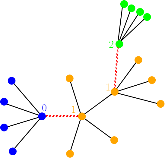
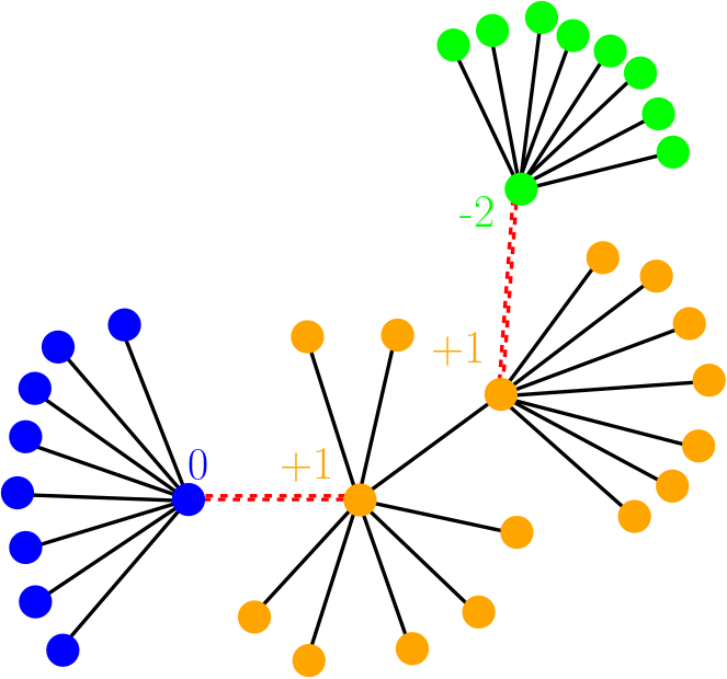
Figure 1. Ground state configurations with $d_{\max}=1$ (same colors denote same spin values, dashed lines denote broken bonds): (Left) for the 3-Potts model. The above configurations are ground states for $d\geq 4$ (see the proof of Corollary 2). (Right) for the SOS model, with $p=1,M=3$. The above configuration is a ground state for $d\geq 8$ (see the proof of Corollary 1).

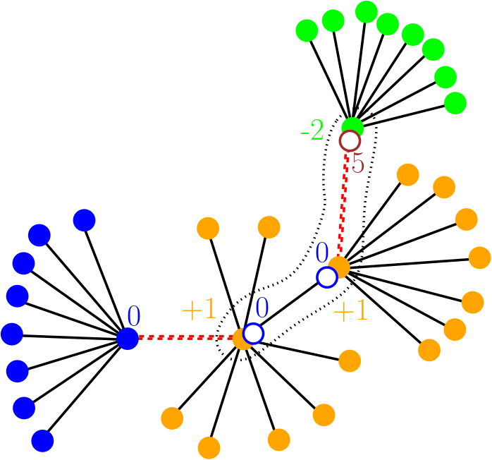
Figure 2. A contour $\bar{\gamma}=(\gamma,\omega_{\gamma})$ relative to the ground state $\omega^{0}$ of Figure 1. The configuration $\omega^{0}$ is depicted by full circles. The support $\gamma$ consists of 3 sites surrounded by a dotted line. The configuration $\omega_{\gamma}$ is depicted by open circles.

3.1. Stable inhomogeneous ground states for the p-SOS models

Consider the homogeneous $p$-SOS-models defined in (2.2), for $d\geq 2$.

Definition 2.

We say that a configuration $\omega^{0}\in\Omega$ is stable with stability constant $c>0$ if for all configurations $\omega\in\Omega$ differing from $\omega^{0}$ at finitely many sites, the excess energy relative to $\omega^{0}$ satisfies the lower bound

$$\begin{split}&H(\omega)-H(\omega^{0})\geq c\sum_{v}|\omega_{v}-\omega^{0}_{v}|^{p}.\end{split}$$ (3.1)

In particular, all stable configurations are ground states in the usual sense that finite volume perturbations raise the energy.

This notion will allow to perform the large-$\beta$ expansions around stable $\omega^{0}$ of Section 4, as we will see. To formulate the lemma on the excess energy and develop a viable criterion on the type of ground states which are stable, consider a pair of configurations $(\omega,\omega^{0})$ which differ on a contour $\bar{\gamma}$. The following notations are useful. Describe the geometric part $\gamma$ of a contour to be a finite subtree rooted at the origin $0$. We think of it embedded into the full tree which we describe as rooted tree which has $d+1$ offspring at the origin, but offspring $d$ at all other sites. By homogeneity of the tree and of the potential, there is no loss in doing so. We write $w\leftarrow v$ if $w$ is a child (or offspring) of $v$ on the full tree relative to the chosen root. We write $k_{v}$ for the number of children of $v$ in the contour $\gamma$. For $v\neq 0$ we have $k_{v}\in\{0,1,\dots,d\}$, while $k_{0}\in\{0,\dots,d+1\}$.

Now we present the lemma on the excess energy of a spin configuration $\omega$ relative to a general ground state $\omega^{0}\in{\mathbb{Z}}^{V}$.

Lemma 1.

Let $p\in(0,\infty)$, $\omega^{0}\in{\mathbb{Z}}^{V}$, and $\omega=\omega_{\gamma}\omega^{0}_{\gamma^{c}}$ such that $\bar{\gamma}=(\gamma,\omega_{\gamma})$ is a contour with respect to the fixed configuration $\omega^{0}$.

Then the excess energy satisfies

$$\begin{split}&H(\omega)-H(\omega^{0})=\sum_{v\in\gamma,w\leftarrow v}\Bigl{(}|\omega_{v}-\omega_{w}|^{p}-|\omega^{0}_{v}-\omega^{0}_{w}|^{p}\Bigr{)}\cr&\geq(dc_{p}^{2}-1)\sum_{v\in\gamma}|\omega_{v}-\omega^{0}_{v}|^{p}-(c_{p}+1)\sum_{v\in\gamma,w\leftarrow v}|\omega^{0}_{v}-\omega^{0}_{w}|^{p}\end{split}$$ (3.2)

where $c_{p}=\min\{2^{1-p},1\}$.

Corollary 1.

For each interaction exponent $p>0$, each maximal increment size $M\in{\mathbb{N}}_{0}$, and each maximal internal degree ${d_{\max}}\in{\mathbb{N}}_{0}$ there is a minimal degree $d(p,M,{d_{\max}})$ such that for all $d\geq d(p,M,{d_{\max}})$ all configurations $\omega^{0}\in{\mathcal{G}}^{0}({d_{\max}},M)$ are stable ground states.

Proof of Corollary 1.

By Lemma 1,

$$\begin{split}&H(\omega)-H(\omega^{0})\geq(dc_{p}^{2}-1-(c_{p}+1)d_{\max}M^{p})\sum_{v\in\gamma}|\omega_{v}-\omega^{0}_{v}|^{p}.\end{split}$$ (3.3)

Thus by taking $d(p,M,{d_{\max}})=1+\lfloor c_{p}^{-2}+(c_{p}^{-1}+c_{p}^{-2}){d_{\max}}M^{p}\rfloor,$ this implies stability with the constant $c:=dc_{p}^{2}-1-(c_{p}+1)d_{\max}M^{p}>0$. ∎

Remark. We may also work with a more general mixed sparsity requirement on $\omega^{0}$ of the form

$$\begin{split}&(dc_{p}^{2}-1)>(c_{p}+1)\sup_{v}\sum_{w\sim v}|\omega^{0}_{v}-\omega^{0}_{w}|^{p}\end{split}$$ (3.4)

which follows from the right hand side of (LABEL:XSpSOS2), and which will provide good bounds to ensure convergence of the cluster expansion, when multiplied with a sufficiently large $\beta$, see below.

Remark. In the particular case of ground state increments bounded in modulus by $M=1$, and sparse set of broken bonds with $d_{D}=1$, we get the minimial degree of $d(p,1,1)=4$, as for the Ising model in [27], for all $p\leq 1$. For the discrete Gaussian (2-SOS model) we get $d(2,1,1)=11$.

Proof.

Let us write

$$s_{v}:=\omega_{v}-\omega^{0}_{v}$$

for the deviation of the spin from the ground state. As $\gamma$ is the support of the contour we have $s_{v}\neq 0$ for $v\in\gamma$ and $s_{w}=0$ for $w\not\in\gamma$. Note that

$$\begin{split}\inf_{s\in{\mathbb{R}}}(|s+t|^{p}+|s|^{p})=c_{p}|t|^{p}\end{split}$$ (3.5)

where, by scaling $c_{p}=\inf_{s\in{\mathbb{R}}}(|s+1|^{p}+|s|^{p})$.

For the standard SOS-model with $p=1$ this becomes the triangle inequality. The infimum in the formula of $c_{p}$ is achieved either at $0$ or $-1/2$ and hence $c_{p}=\min\{2^{1-p},1\}$. Using this twice we obtain

$$\begin{split}|\omega_{v}-\omega_{w}|^{p}&=|s_{v}-s_{w}+(\omega^{0}_{v}-\omega^{0}_{w})|^{p}\cr&\geq c_{p}|s_{v}+(\omega^{0}_{v}-\omega^{0}_{w})|^{p}-|s_{w}|^{p}\cr&\geq c^{2}_{p}|s_{v}|^{p}-c_{p}|\omega^{0}_{v}-\omega^{0}_{w}|^{p}-|s_{w}|^{p}.\cr\end{split}$$ (3.6)

We have

$$\begin{split}&\sum_{v\in\gamma,w\leftarrow v}\Bigl{(}c_{p}^{2}|s_{v}|^{p}-|s_{w}|^{p}\Bigr{)}\cr&=(d+1)c_{p}^{2}|s_{0}|^{p}+(dc_{p}^{2}-1)\sum_{v\in\gamma\backslash 0}|s_{v}|^{p}\geq(dc_{p}^{2}-1)\sum_{v\in\gamma}|s_{v}|^{p}.\end{split}$$ (3.7)

From this the claim follows. ∎

3.2. Stable inhomogeneous ground states for finite-state models

In the case of finite-state ferromagnetic models defined in (2.3), the boundedness of increments is automatic, and the notion of stability becomes the following.

Definition 3.

In our finite-state cases with potentials (2.3) we say that a configuration $\omega^{0}\in\Omega$ is stable with stability constant $c>0$ if for all $\omega\in\Omega$ which differ at most at finitely many sites from $\omega^{0}$, we have the lower bound

$$\begin{split}&H(\omega)-H(\omega^{0})\geq c\sum_{v}1_{\omega_{v}\neq\omega^{0}_{v}}.\end{split}$$ (3.8)

We then have the following analogue of Lemma 1.

Lemma 2.

Consider the finite-state models (2.3). Let $\bar{\gamma}=(\omega_{\gamma},\gamma)$ be a contour relative to the fixed ground state $\omega^{0}$. Denote $\omega=(\omega_{\gamma}\omega^{0}_{\gamma^{c}})$ the corresponding excited spin configuration.

Then the excess energy satisfies

$$\begin{split}&H(\omega)-H(\omega^{0})=\sum_{v\in\gamma,w\leftarrow v}\Bigl{(}\Phi(\omega_{v},\omega_{w})-\Phi(\omega^{0}_{v},\omega^{0}_{w})\Bigr{)}\cr&\geq(d-1)u|\gamma|-\sum_{v\in\gamma,w\leftarrow v}\Bigl{(}\Phi(\omega^{0}_{v},\omega^{0}_{w})+u1_{\omega^{0}_{v}\neq\omega^{0}_{w}}\Bigr{)}\cr&\geq((d-1)u-d_{D}(U+u))|\gamma|.\end{split}$$ (3.9)

Proof.

As $\gamma$ is the support of the contour we have $\omega_{v}\neq\omega^{0}_{v}$ for $v\in\gamma$ and $\omega_{w}=\omega^{0}_{w}$ for $w\not\in\gamma$.

First, realize that

$$\begin{split}\Phi(\omega_{v},\omega_{w})\geq u1_{\omega_{v}\neq\omega^{0}_{v}}-u1_{\omega_{w}\neq\omega^{0}_{w}}-u1_{\omega^{0}_{v}\neq\omega^{0}_{w}}.\end{split}$$ (3.10)

To see this write the inequality in the equivalent form

$$\begin{split}\Phi(\omega_{v},\omega_{w})+u1_{\omega^{0}_{v}\neq\omega^{0}_{w}}+u1_{\omega_{v}=\omega^{0}_{v}}\geq u1_{\omega_{w}=\omega^{0}_{w}}.\end{split}$$ (3.11)

The inequality trivially holds when the r.h.s. equals zero, so let us assume $\omega_{w}=\omega^{0}_{w}$. In the subcase $\omega_{v}=\omega^{0}_{v}$ the inequality obviously holds. In the subcase $\omega_{v}\neq\omega^{0}_{v}$ it is impossible that the two first terms on the l.h.s. reach zero at the same time. This proves the claim (3.10).

Hence we have

$$\begin{split}&\sum_{v\in\gamma,w\leftarrow v}\Bigl{(}1_{\omega_{v}\neq\omega^{0}_{v}}-1_{\omega_{w}\neq\omega^{0}_{w}}\Bigr{)}\cr&=(d+1)1_{\omega_{0}\neq\omega^{0}_{0}}+(d-1)\sum_{v\in\gamma\backslash 0}1_{\omega_{v}\neq\omega^{0}_{v}}\geq(d-1)|\gamma|.\end{split}$$ (3.12)

From the last two inequalities the claim (LABEL:XSfinite) follows. ∎

Corollary 2.

For each interaction constants $u,U$, and each maximal internal degree ${d_{\max}}\in{\mathbb{N}}_{0}$ there is a minimal degree $d(u,U,{d_{\max}})$ such that for all $d\geq d(u,U,{d_{\max}})$, all configurations $\omega^{0}\in{\mathcal{G}}^{0}_{q}({d_{\max},d})$ are stable ground states.

Proof of Corollary 2.

Take

$$d(u,U,{d_{\max}})=2+\lfloor d_{\max}(u+U)/u\rfloor$$

Then indeed

$$(d-1)u-d_{\max}(u+U)=:c>0$$

which by Lemma 2 implies stability with the constant $c$. Note that $d(u,U,{d_{\max}})$ does not depend on $q$. ∎

4. Properties of low-temperature states

Low temperature expansions on trees have unusual properties, as compared to similar expansions on lattices.

First, there is the lack of limiting free energies, which is another way of saying that boundary terms are not smaller than volume terms. In particular, this provocates the failure of variational principles for Gibbs measures on trees (see e.g. [15], also [23], Remarks 3.11, for a valid "inner" variational principle). Next, on trees the complement of a support of a contours is never a connected set, and there are never interior connected components. This facilitates the extension of Peierls argument to not necessarily symmetric frameworks, as we discuss in Section LABEL:sec-tightness.

All of this requires care in proper handling when it comes to more subtle properties, see e.g. the decorrelation property (LABEL:decorr) for unbounded support sets, which we use to prove extremality, after having properly introduced specific cutsets to take care of possibly atypical tail-events of unbounded support. We thus need to be precise to ensure convergence in particular in the case of unbounded spin models, and especially as we do not have homogeneity of our ground states.

4.1. p-SOS models: Proof of Theorem 1

4.1.1. Convergence proof for the partition function

We now turn to the proof of convergence of cluster expansion in the case of the $p$-SOS model, assuming, for $\eta>0$ sufficiently large, the lower bound of the form

$$\begin{split}&\beta(H(\omega)-H(\omega^{0}))\geq\eta\sum_{v\in\gamma}|\omega_{v}-\omega^{0}_{v}|^{p}\end{split}$$ (4.1)

with $\bar{\gamma}=(\omega_{\gamma},\gamma)$ a contour relative to the fixed ground state $\omega^{0}$ and $\omega=(\omega_{\gamma}\omega^{0}_{\gamma^{c}})$ the corresponding excited spin configuration. This bound is given by the excess energy Lemma 1.

We start with a polymer partition function representation of the spin partition function in a finite volume $\Lambda$ with boundary condition equal to $\omega^{0}$, which reads

$$\begin{split}Z_{\Lambda}^{\omega^{0}}={\sum_{n\in{\mathbb{N}}}}\sum_{\bar{\gamma}_{1},\dots,\bar{\gamma}_{n}}\prod_{i=1}^{n}\rho(\bar{\gamma}_{i})\end{split}$$ (4.2)

where the sum is over pairwise compatible polymers $\bar{\gamma}$ with activities

$$\rho(\bar{\gamma})=e^{-\beta(H_{\gamma\cup\partial\gamma}(\omega_{\gamma\cup\partial\gamma})-H_{\gamma\cup\partial\gamma}(\omega^{0}_{\gamma\cup\partial\gamma}))}$$

given in terms of the excess energy.

In our case the pairwise compatibility relation $\bar{\gamma}_{1}\sim\bar{\gamma}_{2}$ is equivalent to the separation of their supports, i.e. $\text{dist}(\gamma_{1},\gamma_{2})\geq 2$. Recall that, by definition, the spin configuration on the complement of the union of the supports of the polymers $\cup_{i=1}^{n}\gamma_{i}$ necessarily coincides with the ground state $\omega^{0}$. The aim of the cluster expansion is to write

$$\begin{split}\log Z_{\Lambda}^{\omega^{0}}={\sum_{I}w_{I}}\end{split}$$ (4.3)

as an analytic function in the complex variables $\rho(\bar{\gamma})$ for $\bar{\gamma}\in P_{\Lambda}$ where $P_{\Lambda}$ denotes the set of polymers in the finite volume $\Lambda$ for the given fixed ground state, and $(w_{I})_{I\in\mathbb{N}_{0}^{P_{\Lambda}}}$ are the expansion terms. For fixed multi-index $I$, $w_{I}$ is proportional to

$$\prod_{\bar{\gamma}\in P_{\Lambda}}\rho(\bar{\gamma})^{I(\bar{\gamma})}.$$

We have the following quantitative convergence criterion.

Proposition 3.

For each degree $d\geq 2$ and interaction exponent $p\in(0,\infty)$ there is a finite constant $\eta_{0}(d,p)$ such that for all $\eta\geq\eta_{0}(d,p)$ the cluster expansion converges for all polymer activities in the polydisk

$$\begin{split}|\rho(\bar{\gamma})|\leq\exp\left(-\eta\sum_{v\in\gamma}|\omega_{v}-\omega^{0}_{v}|^{p}\right)\end{split}$$ (4.4)

for all $\bar{\gamma}$.

Fix a ground state $\omega^{0}$. Let $U\subset W$ be two finite nested volumes. We say that there is an $(U,W)$-cutset (w.r.t $\omega^{0}$) in the configuration $\omega$ if every path from $U$ to infinity has a site $v\in W\setminus U$ for which $\omega_{v}=\omega^{0}_{v}$.

First we prove that there are always cutsets around arbitrary large volumes in sufficiently large annuli, with $\mu^{\omega^{0}}$-probability arbitrarily close to one:

Lemma 4.

Let $v$ be an arbitrary vertex and $B(r,v)\subset V$ the ball of radius $r$ and center $v$ on the tree w.r.t. to the graph distance.

Then, for any radius $r$ and $\epsilon>0$ there exists a finite radius $R>r$ such there is a $\big{(}B(r,v),B(R,v)\big{)}$-cutset with $\mu^{\omega^{0}}$-probability at least $1-\epsilon$.

Proof.

Define $N_{v}$ to be the $({\mathbb{N}}_{0}\cup{\{\infty\}})$-valued random variable which gives the size of a contour containing $v$. Clearly, in finite volume with boundary condition $\omega^{0}$, its value is bounded by the size of the finite volume. Let us now derive an exponential bound on the tail which is uniform in the volume, and also holds in infinite volume.

To do so, look at the exponential moment generating function, which we will do first in finite volume $\Lambda$. Rewrite in terms of polymer partition functions for $t>0$ and estimate

$$\begin{split}&\mu^{\omega^{0}}_{\Lambda}(e^{tN_{v}})=\mu_{\Lambda}^{\omega^{0}}(N_{v}=0)+\sum_{\bar{\gamma}:\gamma\ni v}^{\Lambda}\rho(\bar{\gamma})e^{t|\gamma|}\frac{\sum_{n}\sum^{\Lambda}_{\bar{\gamma}_{1},\dots,\bar{\gamma}_{n}\sim\bar{\gamma}}\prod_{i=1}^{n}\rho(\bar{\gamma}_{i})}{\sum_{n}\sum^{\Lambda}_{\bar{\gamma}_{1},\dots,\bar{\gamma}_{n}}\prod_{i=1}^{n}\rho(\bar{\gamma}_{i})}\cr&\leq 1+\sum_{\bar{\gamma}:\gamma\ni v}^{\Lambda}\rho(\bar{\gamma})e^{t|\gamma|}.\cr\end{split}$$ (4.28)

The last line follows, as all the terms inside the polymer partition function in the numerator are contained in the polymer partition function in the denominator. Decomposing the contour sum in the last line over contours of size $l$ and using the entropy estimate as above, the r.h.s. of the last display is bounded above by

$$\begin{split}1+\sum_{l=1}^{\infty}(d+1)^{2(l-1)}\Bigl{(}\sum_{r\in{\mathbb{Z}}\backslash 0}e^{-|r|^{p}\eta}\Bigr{)}^{l-1}e^{tl}=:L(t).\cr\end{split}$$ (4.29)

$L(t_{0})$ is clearly finite for any choice of $t_{0}$ such that the geometric $l$-sum converges, i.e. s.t.

$$\begin{split}\sum_{l=1}^{\infty}(d+1)^{2}\sum_{r\in{\mathbb{Z}}\backslash 0}e^{-|r|^{p}\eta}e^{t_{0}}<1.\cr\end{split}$$ (4.30)

Assuming such a choice for $t_{0}$, we deduce by the Markov inequality the uniform exponential upper bound on the size-distribution of the contour containing $v$:

$$\begin{split}&\mu^{\omega^{0}}_{\Lambda}(N_{v}\geq N)\leq L(t_{0})e^{-Nt_{0}}\end{split}$$ (4.31)

which extends also to the infinite-volume measure.

We may use this exponential bound on the contour size distribution to control the non-existence event of a cutset in an annulus. To see this, consider contours anchored at the boundary of the inner volume $B(r,v)$ and note

$$\begin{split}&\mu^{\omega^{0}}(\text{there is no cutset in }B(R,v)\backslash B(r,v))\cr&\leq\mu^{\omega^{0}}(\text{there is site }w\in\partial B(r,v):N_{w}\geq R-r)\cr&\leq|\partial B(r,v)|L(t_{0})e^{-(R-r)t_{0}}\end{split}$$ (4.32)

This can be made smaller than $\epsilon$ by chosing $R$ large enough, which proves Lemma 4. ∎

Correlation decay for events of polymer type. We start with correlation bounds for events which can be nicely expressed in terms of contours and polymer partition functions. We say that a local event $A\in{\mathcal{F}}_{W}$ is of polymer-type with supporting set $W$, if $\omega\in A$ implies that $\omega_{v}=\omega^{0}_{v}$ for all sites $v$ in the inner boundary of $W$. Of course not every local event is of such a type, for example the event $\{\omega_{v}=\omega^{0}_{v}+1\}$ is not of this form.

Lemma 5.

(Decay of polymer correlations.) For any local events $A\in{\mathcal{F}}_{W}$ and $B\in{\mathcal{F}}_{U}$ of polymer-type we have

$$|\mu^{\omega^{0}}(A\cap B)-\mu^{\omega^{0}}(A)\mu^{\omega^{0}}(B)|\leq\phi\bigl{(}|W|,d(W,U)\bigr{)}$$

with a decay function of the form $\phi(|W|,r)\leq\exp(C|W|e^{-cr})-1$, for $C,c>0$.

Remark. Note that the estimate is uniform in the size of one of the volumes, which is here chosen to be $|U|$.

Proof.

The proof of the lemma follows by expressing the events $A,B$ in question as unions over events formulated in terms of two finite polymer families, one of the families with supports inside of $W$, the other one in $U$ respectively.

Let us write for short $\mu$ for the infinite-volume measure $\mu^{\omega_{0}}$. We have for the probability of a single contour $a$ the expression

$$\mu(a)=\rho(a)\exp(-\sum_{I\not\sim a}w_{I}).$$

The similar expression for a family of contours reads

$$\mu(a_{1},\dots,a_{l})=\prod_{i=1}^{l}\rho(a_{i})\exp(-\sum_{I:\exists i\in\{1,\dots,l\}:I\not\sim a_{i}}w_{I}).$$

This gives for the correlation between two families of contours with disjoint supports

$$\begin{split}&\mu(a_{1},\dots,a_{l},b_{1},\dots,b_{m})-\mu(a_{1},\dots,a_{l})\mu(b_{1},\dots,b_{m})\cr&=\prod_{i=1}^{l}\rho(a_{i})\prod_{j=1}^{l}\rho(b_{i})\Bigl{(}\exp(-\sum_{I:\exists c\in\{a_{1},\dots,a_{l},b_{1},\dots,b_{m}\}:I\not\sim c}w_{I})\cr&-\exp(-\sum_{I:\exists i\in\{1,\dots,l\}:I\not\sim a_{i}}w_{I})\exp(-\sum_{I:\exists j\in\{1,\dots,m\}:I\not\sim b_{i}}w_{I})\Bigr{)}\end{split}$$ (4.33)

which can be rewritten as

$$\mu(a_{1},\dots,a_{l})\mu(b_{1},\dots,b_{m})\Bigl{(}\exp(-\sum_{I:\exists c\in\{a_{1},\dots,a_{l},b_{1},\dots,b_{m}\}:I\not\sim c}w_{I}$$

$$\hskip 113.81102pt+\sum_{I:\exists i\in\{1,\dots,l\}:I\not\sim a_{i}}w_{I}+\sum_{I:\exists j\in\{1,\dots,m\}:I\not\sim b_{i}}w_{I})-1\Bigr{)}$$ (4.34)

$${=\mu(a_{1},\dots,a_{l})\mu(b_{1},\dots,b_{m})\Bigl{(}\exp(+\sum_{I:\exists(i,j)\in\{1,\ldots,\ell\}\times\{1,\ldots,m\}:I\not\sim\{a_{i},b_{j}\}}w_{I})-1\Bigr{)}}$$ (4.35)

This means that only clusters $I$ are surviving which connect the supporting sets $W$ and $U$, which are controlled by the number of anchoring points in $|W|$ and the cluster expansion estimates. By (LABEL:66), the argument of the above exponential term is indeed bounded by

$$\sum_{w\in W}\sum_{\begin{subarray}{c}\gamma\ni w:\\ |\gamma|\geq d(W,U)\end{subarray}}\sum_{I\ni\gamma}w_{I}$$ (4.36)

$$\leq L(\delta)|W|\sum_{\ell=d(W,U)}^{\infty}(d+1)^{2(\ell-1)}\left(\sum_{r\in{\mathbb{Z}}\backslash 0}e^{(-\eta+A)|r|^{p}}\right)^{\ell}$$ (4.37)

$$\leq|W|C(\delta,d)e^{-c(d,\eta)d(W,U)}.$$ (4.38)

This delivers the existence of the decay function $\phi$ with the promised property such that

$$\begin{split}&\mu(a_{1},\dots,a_{l},b_{1},\dots,b_{m})-\mu(a_{1},\dots,a_{l})\mu(b_{1},\dots,b_{m})\cr&\leq\mu(a_{1},\dots,a_{l})\mu(b_{1},\dots,b_{m})\phi(|W|,{d(W,U)}).\end{split}$$ (4.39)

Finally note that the estimate survives the summation over all possible different families of contours inside $W,U$ (which form the decomposition of the events $A,B$), as the prefactors sum up at most to $1$. Indeed, let $A=A_{W}\times\Omega_{0}^{W^{c}}\in\mathcal{F}_{W}$ and $B=B_{U}\times\Omega_{0}^{U^{c}}\in\mathcal{F}_{U}$, then

$$|\mu(A\cap B)-\mu(A)\mu(B)| =|\sum_{\omega_{W}\in A_{W}}\sum_{\eta_{U}\in B_{U}}\mu(\omega_{W}\eta_{U})-\mu(\omega_{W})\mu(\eta_{U})|$$ (4.40)

$$\leq\sum_{\omega_{W}\in A_{W}}\sum_{\eta_{U}\in B_{U}}\mu(\omega_{W})\mu(\eta_{U})\phi(|W|,d(W,U))$$ (4.41)

$$\leq\phi(|W|,d(W,U)).$$ (4.42)

This proves Lemma 5. ∎

Extremality via decorrelation of general events via cutsets. We turn to the proof of extremality of the above constructed measures $\mu^{\omega_{0}}$. By [Proposition 7.9] of [32], it is equivalent to show the following

Proposition 4.

For any fixed $A\in{\mathcal{F}}$, and cofinal volume sequence $(\Lambda_{n})_{n\in{\mathbb{N}}}$ the decorrelation property holds

$$\begin{split}&\lim_{n\to\infty}\sup_{B\in{\mathcal{F}}_{\Lambda^{c}_{n}}}|\mu^{\omega^{0}}(A\cap B)-\mu^{\omega^{0}}(A)\mu^{\omega^{0}}(B)|=0.\end{split}$$ (4.43)

Remark 2.

Indeed, from (LABEL:decorr) the tail-triviality of $\mu=\mu^{\omega^{0}}$ follows by taking $A=B$ to be a tail-event. This is an allowed choice in the above limit statement, which delivers the desired formula $\mu(A)=\mu(A)^{2}$.

Proof.

Spelling out the above general decorrelation property we are aiming at, means that for any $A\in\mathcal{F}$ and $\delta>0$ there exists $n_{0}(A,\delta)\in{\mathbb{N}}$ such that for all $n\geq n_{0}$ we have for any $B\in{\mathcal{F}}_{\Lambda^{c}_{n}}$

$$\begin{split}&|\mu(A\cap B)-\mu(A)\mu(B)|\leq\delta.\end{split}$$ (4.44)

To see this, we apply the semi-ring approximation theorem twice, and condition on the presence of suitable cutsets, as follows. Note first that by the semi-ring approximation theorem applied to the semi-ring of cylinder events, for any $\epsilon>0$ and any event $A{\in\mathcal{F}}$ we may choose a cylinder event $A_{\epsilon}$ such that $\mu(A\triangle A_{\epsilon})\leq\epsilon$. See e.g. the book of Klenke [36], Theorem 1.65 (ii).

It is now elementary that we can choose $\epsilon>0$ small enough such that for any four events for which $\mu(A\triangle A_{\epsilon})\leq\epsilon$ and $\mu(B\triangle B_{\epsilon})\leq\epsilon$ we always have

$$\begin{split}|\mu(A;B)-\mu(A_{\epsilon};B_{\epsilon})|\leq\delta/2\end{split}$$ (4.45)

where $\mu(A;B):=\mu(A\cap B)-\mu(A)\mu(B)$. (The choice of $\epsilon=\frac{\delta}{{8}}$ will do for this). Given $A\in\mathcal{F}$, let us fix the cylinder set $A_{\epsilon}$ which is obtained in such a way. It then suffices to show that there exists $n_{1}=n_{1}(A_{\epsilon},\delta)\in{\mathbb{N}}$ such that for all $n\geq n_{1}$ for any cylinders $B_{\epsilon}\in{\mathcal{F}}_{\Lambda^{c}_{n}}$ we have

$$\begin{split}&|\mu(A_{\epsilon};B_{\epsilon})|\leq\delta/2.\end{split}$$ (4.46)

As the approximating cylinder events $A_{\epsilon},B_{\epsilon}$ may not be of polymer type as introduced above, we can not directly apply the decay estimate of Lemma 5 for those events without further ado. We solve this problem by the introduction of cutsets, which occur with high probability, in the following way depicted in Figure 3.

Fix a vertex $v$, and choose $r_{1}$ s.t. $A_{\epsilon}\in{\mathcal{F}}_{B(r_{1},v)}$. For radii $r_{1}<R_{1}<r_{2}<R_{2}<r_{3}<R_{3}$, consider cutset events of the type

$$C_{i}:=\{\text{there is a cutset in }B(R_{i},v)\backslash B(r_{i},v)\}$$

for $i=1,2,3$. Let us now construct the radii. Fix $\delta^{\prime}>0$, to be chosen below.

Annulus for inner cutset. By Lemma 4, choose $R_{1}>r_{1}$ large enough such that with probability at least $1-\delta^{\prime}$ there is a cutset in the annulus with $r_{1},R_{1}$.

Decorrelation annulus. Given $R_{1}$, by Lemma 5, choose $r_{2}$ large enough such that $\phi(|B_{R_{1}}|,r_{2}-R_{1})\leq\delta/4$.

Annulus for middle cutset. Choose $R_{2}$ large enough such that with probability at least $1-\delta^{\prime}$ there is a cutset in the annulus with $r_{2},R_{2}$. Choose $n$ large enough such that $\Lambda_{n}\supset B(R_{2},v)$.

Outmost cutset. Let $B_{\epsilon}$ be a cylinder set in ${\mathcal{F}}_{\Lambda^{c}_{n}}$. Choose $r_{3}$ such that $B_{\epsilon}\in{\mathcal{F}}_{B(r_{3},v)}$. Choose $R_{3}$ large enough such that with probability at least $1-\delta^{\prime}$ there is a cutset in the annulus with respective radii $r_{3}$ and $R_{3}$.

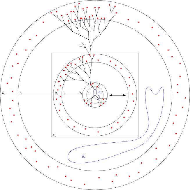
Figure 3. The picture shows the events $A_{\epsilon}^{\prime}$ and $B_{\epsilon}^{\prime}$ on the binary tree where $d=2$: in blue are the supports of the cylinder events $A_{\epsilon}$ (inside the ball of radius $r_{1}$) and $B_{\epsilon}$ (inside the ball of radius $r_{3}$ and outside the box $\Lambda_{n}$). The (larger) red dots represent sites $v$ on the cutsets where $\sigma_{v}=\omega^{0}_{v}$. The decorrelation annulus (between radii $R_{1}$ and $r_{2}$) is emphasized with a bold arrow.

Now define the following events, as depicted on Figure 3:

$$A^{\prime}_{\epsilon}:=A_{\epsilon}\cap C_{1},\qquad B^{\prime}_{\epsilon}:=B_{\epsilon}\cap C_{2}\cap C_{3}.$$

The advantage of these events is that they are of polymer-type with well-separated supporting sets, and by construction enjoy the decorrelation property

$$\begin{split}&|\mu(A^{\prime}_{\epsilon};B^{\prime}_{\epsilon})|\leq\delta/4.\end{split}$$ (4.47)

Noting that $\mu(A^{\prime}_{\epsilon}\triangle A_{\epsilon})\leq\delta^{\prime}$ and $\mu(B^{\prime}_{\epsilon}\triangle B_{\epsilon})\leq 2\delta^{\prime}$ by the construction of the width of the radii for the cutsets, we now assume a choice of $\delta^{\prime}$ has been made such that

$$\begin{split}&|\mu(A^{\prime}_{\epsilon};B^{\prime}_{\epsilon})-\mu(A_{\epsilon};B_{\epsilon})|\leq\delta/4.\end{split}$$ (4.48)

$\delta^{\prime}=\frac{\delta}{48}$ will do for this. This finishes the proof of Proposition 4. ∎

4.2. Finite-spin models: Proof of Theorem 2

We discuss the corresponding proofs for the finite-spin models defined in (2.3). We are assuming the lower bound of the form

$$\begin{split}&\beta(H(\omega)-H(\omega^{0}))\geq\zeta|\gamma|\end{split}$$ (4.49)

with $\zeta>0$, which is provided by Lemma 2 for the excess energy with respect to configurations $\omega^{0}$ which are elements in the set of stable ground states ${\mathcal{G}}^{0}_{q}(d_{D})$, which was defined in the statement of Theorem 2.

The definition of labelled contours $\bar{\gamma}$ w.r.t. a fixed stable reference ground state $\omega^{0}$ stays the same, i.e. they are connected sets of incorrect points, together with the spin values on these sets. We are again using representations in terms of polymer partition functions in which the contours carry activities

$$\rho(\bar{\gamma})=e^{-\beta(H_{\gamma\cup\partial\gamma}(\omega_{\gamma\cup\partial\gamma})-H_{\gamma\cup\partial\gamma}(\omega^{0}_{\gamma\cup\partial\gamma}))}$$

given in terms of the excess energy.

We first prove a convergence criterion for the low-temperature expansions, which parallels Proposition 3, but assumes only volume-suppression for contour-activities in the following form.

Proposition 5.

For each degree $d\geq 2$ and $q\in(2,\infty)$ there is a finite constant $\zeta_{0}(d,p)$ such that for all $\zeta\geq\zeta_{0}(d,p)$ the cluster expansion converges for all complex polymer activities in the polydisk

$$\begin{split}|\rho(\bar{\gamma})|\leq\exp\left(-\zeta|\gamma|\right)\end{split}$$ (4.50)

for all $\bar{\gamma}$.

Remark. Note that the r.h.s. depends only on the volume $|\gamma|$ of the labelled contour $\bar{\gamma}$, as opposed to the configuration-dependent assumption in Proposition 3. Such uniformity in the spin configuration on $\gamma$ is only possible for finite-spin models.

Proof.

We choose the generalized volume function $b$ for labelled contours in the application of Theorem 1 of Bovier-Zahradník ([14], Theorem 1, page 768), only depending on the volume of the contour in the form

$$\begin{split}&b(\bar{\gamma})=B|\gamma|\end{split}$$ (4.51)

where the prefactor $B>0$ can be chosen to our convenience, see below.

Rerunning the convergence proof for the partition function as before, we see the following. The first condition (LABEL:Condi1) is satisfied for $e^{B}\leq\delta e^{\zeta}$, by the assumption (4.50). The second condition (LABEL:Condi2) is now implied if we have

$$\begin{split}(d+2)\sum_{l=1}^{\infty}e^{-l(\zeta-B)}(q-1)^{l}(d+1)^{2(l-1)}\leq\frac{B}{L(\delta)}.\end{split}$$ (4.52)

Note that the number of choices of spin-values per site on the contour support is $q-1$, which is responsible for its appearance on the l.h.s. of (4.52) above. We may finally choose $B=1,\delta=\frac{1}{2}$ to see that we satisfy both conditions by choosing $\zeta$ large enough. This proves Proposition 5. ∎

Having seen this, the remaining parts of the proof of the main theorem all carry over from the $p$-SOS analogues. This including convergence via Fourier transform (while tightness is automatic), polymer decorrelation, and finally the extremality of the measures $\mu^{\omega^{0}}$ via the general correlation decay of Proposition 4, which holds by means of the Lemma 4 on cutsets. We finally remark that from (4.52) follows that for the $q$-state Potts model we have a bound on the minimal inverse temperature $\beta$ for which all low-temperature states exist, on the order of $\log(q-1)$.

This provides the proof of Theorem 2.

Remark. We are not after optimality of the degree $d$ of the tree for which our states exist. It may be possible to extend the construction in the $p$-SOS and finite-spin cases to include also trees of low degree, even the binary tree, by demanding the distance between broken bonds in the ground state to be large. This has been outlined for the particular case of foliated states for the Ising model on binary trees in [28], whether it can be done for our models we leave for future work.

5. Applications to inhomogeneous systems with local disorder terms

5.1. Models

Let us consider our previously discussed ${\mathbb{Z}}_{q}$-valued or ${\mathbb{Z}}$-valued models with homogeneous pair interactions $\Phi$, defined in (2.2) and (2.3), but under the additional influence in the interaction of single-site terms $\Psi_{v}:\Omega_{0}\rightarrow{\mathbb{R}}$ at the sites $v\in V$. So the Hamiltonian now takes the following form

$$\begin{split}\sum_{v\sim w}\Phi(\omega_{v},\omega_{w})+\sum_{v}\Psi_{v}(\omega_{v}).\end{split}$$ (5.1)

It is in general spatially inhomogeneous, but the case $\Psi_{v}=\Psi$ of a homogeneous local potential is not excluded, and already of interest. Let us highlight some prototypical special cases.

${\mathbb{Z}}_{q}$-valued Potts model in quenched random potentials, random field Ising model

As before we write the pair potential of the Potts model in the form $\Phi(\omega_{v},\omega_{w})=1_{\omega_{v}\neq\omega_{w}}$. Moreover, the single-site term $\Psi_{v}(\cdot)$ is a quenched random potential on ${\mathbb{Z}}_{q}$, which is usually assumed to be i.i.d. over the sites $v\in V$, according to an external probability distribution ${\mathbb{P}}$, and studied w.r.t. to its ${\mathbb{P}}$-a.s. properties. The case of a deterministic single-site interaction where $\Psi_{v}(\cdot)=\Psi(\cdot)$ is allowed and models the Potts model in a homogeneous vector-valued field.

The subcase $q=2$ is identical to the random field Ising model (RFIM) for spins $\omega_{v}\in\{-1,1\}$, and quenched random fields $\eta_{v}\in{\mathbb{R}}$, with Hamiltonian

$$-\sum_{v\sim w}\omega_{v}\omega_{w}-\sum_{v}\eta_{v}\omega_{v}$$

which was already considered on the tree by Bleher et al. [12]. These authors proved in particular that for the RFIM in the low temperature (large $\beta$) regime, there is a strictly positive maximal strength $\eta^{*}(\beta)>0$ such that for all random field configurations $\eta=(\eta_{v})_{v\in V}$ with $\sup_{v\in V}|\eta_{v}|\leq\eta^{*}(\beta)$ there are at least two different $\eta$-dependent Gibbs measures $\mu^{+}[\eta],\mu^{-}[\eta]$. These infinite-volume measures are obtained as weak limits of the finite-volume measures with all-plus (all-minus) boundary conditions. In their result the actual distribution under ${\mathbb{P}}$ plays no role.
We are aiming in this section at a broad generalization of this statement to extremal measures $\mu^{\omega^{0}}[\eta]$ constructed with non-homogeneous spin-boundary conditions $\omega^{0}$, and the more general model classes under discussion here.

${\mathbb{Z}}$-valued random field random surface models: random field $p$-SOS model

In this variation of the $p$-SOS model the Hamiltonian takes the form

$$\begin{split}\sum_{v\sim w}|\omega_{v}-\omega_{w}|^{p}+\sum_{v}\eta_{v}\omega_{v}\end{split}$$ (5.2)

with quenched random fields $\eta_{v}\in{\mathbb{R}}$ and spins $\omega_{v}\in{\mathbb{Z}}$. Note that the local disorder term of random-field type adds an unbounded perturbation to the Hamiltonian, even for uniformly bounded random fields $\eta_{v}$. The model is well-defined for $p\geq 1$, while the case $p<1$ would lead to infinite partition functions for non-zero external fields. It has been recently studied in detail on the lattice for $p=2$ in [17] with a focus on the case where $(\eta_{v})_{v\in V}$ are symmetrically distributed i.i.d. quenched random variables which have mean zero and finite variance. The authors obtained in their work upper and lower bounds on disorder-averages of the gradient fluctuations $|\omega_{v}-\omega_{w}|^{2}$ w.r.t. to the finite-volume zero-boundary condition Gibbs measure $\mu^{0}_{\Lambda}[\eta]$, valid for all finite boxes $\Lambda$. They provide boundedness of gradient fluctuations uniformly in the box-size in $d\geq 3$, and roughening of local fluctuations in $d\leq 2$.

Continuous-spin versions of the model with spin values $\omega_{v}\in{\mathbb{R}}$, also thereby allowing more general pair-interactions, were studied in [17, 16]. We point out that the model (5.2) is of gradient-type, due to the multiplicative nature of the local terms, which opens the field for the study of Gradient Gibbs measures in the infinite volume which are defined on configurations of heights modulo a joint height shift, with state-space ${\mathbb{Z}}^{V}/{\mathbb{Z}}$.

${\mathbb{Z}}$-valued p-SOS models in random media

Here one keeps the gradient interaction, but allows more general local interactions, so that the Hamiltonian becomes

$$\begin{split}\sum_{v\sim w}|\omega_{v}-\omega_{w}|^{p}+\sum_{v}\zeta_{v}(\omega_{v})\end{split}$$ (5.3)

where $(\zeta_{v}(k))_{v\in V,k\in{\mathbb{Z}}}$ are real numbers. This model has been studied on the lattice ${\mathbb{Z}}^{d}$ for $p=1$ in [13] under the assumption that $\eta=(\zeta_{v}(k))_{v\in V,k\in{\mathbb{Z}}}$ is a process of i.i.d. random variables. As main result the existence of infinite-volume Gibbs measures $\mu^{0}[\eta]$ obtained with zero-boundary conditions was shown for small disorder, large inverse temperature in lattice dimensions $d\geq 3$. The proof was based on a rigorous renormalization group analysis using multiscale cluster expansions.

Let us consider the above perturbed models on the regular tree and present two stability theorems.

5.2. Stability Theorems

Theorem 6.

Let $p\geq 1$ and consider the $p$-SOS models (2.2) under the assumptions of Theorem 1 formulated for the model without disorder.

Consider now the model in the additional presence of quenched random fields $\eta=(\eta_{v})_{v\in V}$ with Hamiltonian (5.2). Then there is a strictly positive threshold $\delta^{*}>0$ such that for each $\eta$ satisfying

$$\begin{split}\sup_{v\in V}|\eta_{v}|\leq\delta^{*}\end{split}$$ (5.4)

at $\beta$ sufficiently large, there is an identifiable class of extremal Gibbs measures $\mu^{\omega^{0}}_{\beta}[\eta]$, concentrated on the stable ground states $\omega^{0}$, as described in Theorem 1.

Remark: Note that the case of a small homogeneous non-zero field is encluded. Note also that $\delta^{*}$ provided by the theorem depends on the parameters $d,{d_{{\max}}},M$ describing the sparsity and uniform bounds on the increments of the ground states $\omega^{0}$, which were discussed before.

We turn to a corresponding stability result in the remaining classes of disordered models described above.

Theorem 7.

Consider the ${\mathbb{Z}}$-valued $p$-SOS models (2.2) for $p>0$ under the assumptions of Theorem 1 formulated for the model without disorder, but in the presence of additional local perturbations of the form ((5.1)).

Alternatively consider the ${\mathbb{Z}}_{q}$-valued models under the assumptions of Theorem 2 formulated for the model without disorder, but in the presence of additional local perturbations of the form 5.2

Then, for both types of models, there is a strictly positive threshold $\epsilon^{*}>0$ such that for each choice of local potentials $\eta=(\Psi_{v}(\cdot))_{v\in V}$ satisfying

$$\begin{split}\sup_{v\in V}\sup_{k,l\in\Omega_{0}}|\Psi_{v}(k)-\Psi_{v}(l)|\leq\epsilon^{*}\end{split}$$ (5.5)

there is an identifiable class of extremal Gibbs measures $\mu^{\omega^{0}}[\eta]$, concentrated on the stable ground states $\omega^{0}$, as described in Theorem 1 and Theorem 2 respectively.

5.3. Proofs via stability of excess energy estimates

To prove the last two stability theorems it turns out that we can use exactly the same contour definitions and characterizations of ground states in spe, as for the unperturbed models. However, in doing this we need to ensure that the expansions around the ground states $\omega^{0}$ which were identified in the homogeneous models, and their consequences, also stay valid for the $\eta$-perturbed models. This leads us to the study of excess energies in the perturbed models.

Recall for this purpose the definition of stability of a ground state $\omega^{0}$ with a constant $c>0$ given above in the two cases of finite or infinite local state space. We then have the following lemma on the stability in the models perturbed by a collection of local potentials $\eta=(\Psi_{v})_{v\in V}$.

Lemma 6.

Consider ${\mathbb{Z}}$-valued or ${\mathbb{Z}}_{q}$-valued models with additional local potentials of the type (5.1). Assume that $\omega_{0}\in\Omega$ is a ground state which is stable with a constant $c>0$ for the model with $\eta=0$.

• If the single-site potentials obey the smallness condition

  $$\begin{split}\sup_{v\in V}\sup_{k,l\in\Omega_{0}}|\Psi_{v}(k)-\Psi_{v}(l)|=:\epsilon<c\end{split}$$ (5.6)

  then $\omega_{0}\in\Omega$ is a stable ground state with reduced constant $c-\epsilon>0$.

• Consider specifically the random field random surface model (5.2) with $p\geq 1$. If

  $$\begin{split}\sup_{v\in V}|\eta_{v}|=:\delta<c\end{split}$$ (5.7)

  then $\omega_{0}\in\Omega$ is a stable ground state with reduced constant $c-\delta>0$.

Proof.

The statements follow from spelling out the definitions in terms of the excess energies, and the triangle inequality. Note for the second case, that the excess energy of $\omega$ relative to $\omega^{0}$ in the model (5.2) has the lower bound $\sum_{v}(c|\omega_{v}-\omega_{v}^{0}|^{p}-\epsilon|\omega_{v}-\omega_{v}^{0}|)\geq\sum_{v}(c-\epsilon)|\omega_{v}-\omega_{v}^{0}|^{p}$. The estimate works iff $p\geq 1$, which had to be already assumed before to have a well-defined model. This explains the restriction to the case of convex interactions in the $p$-SOS models with random field disorder in the formulation of the lemma and of Theorem 6. ∎

Given Lemma 6 the proof of Theorem 6 and Theorem 7 is straightforward.

References

- [1] H. Akim, U. Rozikov, S. Temir. A new set of limiting Gibbs measures for the Ising model on a Cayley tree. J. Stat. Phys. 142, no 2:314–321, 2011.
- [2] R. Bauerschmidt, J. Park, P.-F. Rodriguez. The Discrete Gaussian model, I. Renormalisation group flow. Preprint arXiv 2202.02286. 2022.
- [3] R. Bauerschmidt, J. Park, P.-F. Rodriguez. The Discrete Gaussian model, II. Infinite-volume scaling limit at high temperature. Preprint arXiv 2202.02287. 2022.
- [4] S. Bergmann, S. Kissel, C. Külske. Dynamical Gibbs-non-Gibbs transitions in Widom-Rowlinson models on trees. Accepted for publication in Annales de l’Institut Henri Poincaré, available on arXiv:2012.09718. 2020.
- [5] H. van Beijeren. Interface Sharpness in the Ising System. Comm. Math. Phys., 40:1–6, 1975.
- [6] M. Biskup, R. Kotecký, H. Spohn. Phase coexistence of gradient Gibbs states. Proba. Th. Relat. Fields 139, no 1-2:1–39, 2007.
- [7] M. Biskup, H. Spohn. Scaling limit for a class of gradient fields with nonconvex potentials. Ann. Proba. 39, no 1:224–251, 2011.
- [8] P. Bleher. Extremity of the disordered phase in the Ising model on the Bethe lattice. Comm. Math. Phys. 128:411-419, 1990.
- [9] P. Bleher, N. Ganikhodjaev. On pure phases of the Ising model on the Bethe lattice. Theo. Prob. Appl. 35:1-26, 1991.
- [10] P. Bleher, J. Ruiz, V. Zagrebnov. On the Phase Diagram of the Random Field Ising Model on the Bethe Lattice. J. Stat. Phys. 93:33–78, 1998.
- [11] P. Bleher, J. Ruiz, R. Schonmann, S. Shlosman, V. Zagrebnov. Rigidity of the critical phases on a Cayley tree. Moscow Math. J. 1, no 3:345–363, 2001.
- [12] P. Bleher, J. Ruiz, V. Zagrebnov. On the purity of the limiting Gibbs state for the Ising model on the Bethe lattice. J. Stat. Phys. 79:473-482, 1995.
- [13] A. Bovier, C. Külske. A rigorous renormalization group method for interfaces in random media. Rev. Math. Phys. 6, no 3:413–496, 1994.
- [14] A. Bovier, M. Zahradník. A simple inductive approach to the problem of convergence of cluster expansions of polymer models. J. Stat. Phys. 100, no3-4:765–778, 2000.
- [15] R. Burton, C-E. Pfister, J. Steif. The variational principle for Gibbs states fails on trees. Mark. Proc. Relat. Fields 1, no 3:387-406, 1995.
- [16] C. Cotar, C. Külske. Existence of random gradient states. Ann. Appl. Proba. 22, no 4:1650–1692, 2012.
- [17] P. Dario, M. Harel, R. Peled. Random-field random surfaces. Preprint arXiv 2021.02199. To appear in Proba. Th. Relat. Fields, 2021+.
- [18] J.-D. Deuschel, G. Giacomin, D. Ioffe. Large deviation and concentration properties for interfaces models. Proba. Th. Relat. Fields 117, no 1:49-111, 2000.
- [19] R. L. Dobrushin. Gibbs States Describing Coexistence of Phases for a Ising Model. Theo. Probab. Appli., 17(4), 1972.
- [20] A. van Enter, V. Ermolaev, G. Iacobelli, C. Külske. Gibbs-non-Gibbs properties for evolving Ising models on trees. Annales de l’Institut Henri Poincaré 48, no 3:774–791, 2012.
- [21] A. van Enter, C. Külske. Nonexistence of random gradient Gibbs measures in continuous interface models in . Ann. Appl. Proba. 18, no 1:109–119, 2008.
- [22] W. Evans, C. Kenyon, Y. Peres, L. Schulman. Broadcasting on trees and the Ising model. Ann. Proba 10, no 2:410–433, 2000.
- [23] H. Föllmer, J. Snell. An “inner” variational principle for Markov fields on a graph. Z. Wahrsch. verw. Geb. 39:187-195, 1977.
- [24] T. Funaki, H. Spohn. Motion by mean curvature from the Ginzburg-Landau interface model. Comm. Math. Phys. 185:1–36, 1997.
- [25] S. Friedli, Y. Velenik. Statistical Mechanics of Lattice Systems: a Concrete Mathematical Introduction. Cambridge University Press, 2017.
- [26] D. Gandolfo, C. Maes, J. Ruiz, S. Shlosman. Glassy states: The free Ising model on a tree. J. Stat. Phys. 180, no 1/6: 227–237, 2020.
- [27] D. Gandolfo, J. Ruiz, S. Shlosman. A manifold of Gibbs states of the Ising model on a Cayley tree. J. Stat. Phys. 148:999–1005, 2012.
- [28] D. Gandolfo, J. Ruiz, S. Shlosman. A manifold of pure Gibbs states of the Ising model on Lobatchevsky plane. Comm. Math. Phys. 334:313–330, 2015.
- [29] F. Henning, C. Külske. Coexistence of localized Gibbs measures and delocalized gradient Gibbs measures on trees. Ann. Appl. Proba. 31, no 5:2284–2310, 2021.
- [30] F. Henning, C. Külske. Existence of gradient Gibbs measures on regular trees which are not translation invariant. Preprint arXiv 2102.11899. To appear in Ann. Appl. Proba. 2022+
- [31] F. Henning, C. Külske, A. Le Ny, U. Rozikov. Gradient Gibbs measures for the SOS-model with countable values on Cayley tree. Elec. J. Proba. 24, 2019.
- [32] H.O. Georgii. Gibbs measures and phase transitions. de Gruyter studies in mathematics, Vol. 9, Berlin–New York, 1988.
- [33] Y. Higuchi. Remarks on the limiting Gibbs states on a (d+1)-tree. Publ. RIMS Kyoto Univ. 13:335-348, 1977.
- [34] D. Ioffe. Extremality of the disordered state for the Ising model on general trees. Workshop in Versailles, B. Chauvin, S. Cohen, A. Rouault Eds, Progr. Probab. 40:3-14, 1996.
- [35] D. Ioffe. On the extremality of the disordered state of the Ising model on the Bethe lattice. Lett. Math. Phys. 37:137-143, 1996.
- [36] A. Klenke. Probability theory, a comprehensive course. Second edition, ser. Universitext. Springer, London 2014.
- [37] R. Kotecký, S. Luckhaus. Nonlinear elastic free energies and gradient Young-Gibbs measures. Comm. Math. Phys. 326:887–917, 2014.
- [38] P. Lammers, S. Ott. Delocalization and absolute-value-FKG in the solid-on-solid model. Preprint 2021. arXiv 2101.05139.
- [39] R. Lyons. The Ising model and percolation on trees and tree-like graphs. Comm. Math. Phys. 125, no 2:337-353, 1989.
- [40] C. Preston. Gibbs states on countable sets. Cambridge tracts in Math. 68, Cambridge University Press, 1974.
- [41] C. Preston. Random Fields. Lecture Notes in Mathematics 534, Springer-Verlag, 1976.
- [42] M. Rakhmatullaev, U. Rozikov. Description of weakly periodic Gibbs measures for the Ising model on a Cayley tree. Theo. Math. Phys. 156, no 2:1218–1227, 2008.
- [43] U. Rozikov. Gibbs measures on Cayley trees. World Scientific, Hackensack, NJ, 2013.
- [44] S. Sheffield. Random surfaces. Astérisque 304, Société Mathématique de France, 2005.
- [45] F. Spitzer. Markov random fields on an infinite tree. Ann. Probab. 3:387-398, 1975.
- [46] Y. Velenik. Localization and delocalization of random interfaces. Proba. Surveys 3:112–169, 2006.
- [47] S. Zachary. Countable state space Markov random fields and Markov chains on trees. Ann. Probab. 11:894-903, 1983.