Constrained Prescriptive Trees via Column Generation

Abstract

With the abundance of available data, many enterprises seek to implement data-driven prescriptive analytics to help them make informed decisions. These prescriptive policies need to satisfy operational constraints, and proactively eliminate rule conflicts, both of which are ubiquitous in practice. It is also desirable for them to be simple and interpretable, so they can be easily verified and implemented. Existing approaches from the literature center around constructing variants of prescriptive decision trees to generate interpretable policies. However, none of the existing methods are able to handle constraints. In this paper, we propose a scalable method that solves the constrained prescriptive policy generation problem. We introduce a novel path-based mixed-integer program (MIP) formulation which identifies a (near) optimal policy efficiently via column generation. The policy generated can be represented as a multiway-split tree which is more interpretable and informative than a binary-split tree due to its shorter rules. We demonstrate the efficacy of our method with extensive experiments on both synthetic and real datasets.

Introduction

With the abundance of available data, many enterprises seek to implement data-driven prescriptive analytics to help them make better decisions. Unlike predictive analytics, which applies mathematical models to forecast potential outcomes, prescriptive analytics determines the best course of action for the future, frequently utilizing the outcome of a predictive model (Lepenioti et al. 2020). For instance, in revenue management, pricing decisions are based on estimated demand learnt from historical sales data; in healthcare, personalized medicine is prescribed based on past patients’ responses towards different treatment options. A key characteristic of prescriptive analytics is the presence of constraints, which is largely missing from predictive analytics. Constraints are ubiquitous in practice: a revenue-maximization problem may limit prices such that the resulting demand does not exceed production capacity; similarly, a patient’s available treatment options may be limited by his or her pre-existing conditions.

Despite machine learning (ML) making huge strides in recent years, there are several obstacles standing in the way of widespread adoption of prescriptive analytics in practice. Firstly, prescriptive analytics often works in conjunction with predictive models, whose output may be nonlinear, non-convex and/or discontinuous (and therefore not differentiable), resulting in intractable downstream optimization problems. To generate meaningful policies, it is critical to embed the myriad of business requirements into the decision optimization problem, exacerbating the computational challenge at hand. Secondly, powerful black-box predictive models inevitably obscure the downstream decision-making process, making it difficult for enterprises to understand and trust the prescribed policies. Meanwhile, recommendations based on these models tend to be highly complex, making implementation and maintenance of these policies challenging and cumbersome.

There have been some recent works studying the problem of generating interpretable prescriptive policy. A common theme is to construct variants of decision trees which represent the prescribed policies, as trees provide “human-friendly” explanations (Frosst and Hinton 2017; Miller 2019). Each path in a tree from the root node to a leaf node corresponds to a policy, and all samples in a leaf are prescribed with a same action. The procedure of generating such a tree-based policy may vary - the prediction step can be either embedded in the policy generation step (Kallus 2017; Bertsimas, Dunn, and Mundru 2019), or explicitly separated from prescription (Zhou, Athey, and Wager 2018; Amram, Dunn, and Zhuo 2020; Biggs, Sun, and Ettl 2021). Meanwhile, the prescriptive tree can be constructed either greedily (Zhou, Athey, and Wager 2018; Biggs, Sun, and Ettl 2021) or optimally (Kallus 2017; Amram, Dunn, and Zhuo 2020). However, none of the existing methods are capable of handling operational constraints which are paramount for successful enterprise adoption of prescriptive analytics - this is the gap which we intend to fill with this work.

In this paper, we propose a scalable method to solve the constrained prescriptive policy generation problem. We consider the predictive teacher and prescriptive student framework (Zhou, Athey, and Wager 2018; Amram, Dunn, and Zhuo 2020; Biggs, Sun, and Ettl 2021), where a predictive model (teacher) is first trained to produce counterfactual outcomes associated with different actions for every sample in the dataset. Based on the counterfactual estimations, the downstream prescriptive model (student) determines the best set of policies to divide the samples that optimizes the given objective. Our key contributions are as follows:

1. Constrained policy prescription To the best of our knowledge, we are the first to propose a prescriptive tree which is capable of handling constraints that span across multiple rules. Existing tree-based approaches in the literature typically produce unconstrained policies that ignore rule conflicts and operational feasibility, severely limiting their usefulness in practice.

2. Novel MIP formulation We model rules or paths in a tree explicitly as it provides a natural way to impose constraints unlike prior MIP methods which rely on arc-based feature-level models. More specifically, we show that the constrained tree-based policy prescription problem can be formulated as a set-partitioning problem with side-constraints. A key challenge here is that the search space for rules may be computationally prohibitive to solve the problem directly for high dimensional datasets. To overcome this hurdle, we implement column generation (Ford Jr and Fulkerson 1958), where promising candidate rules can be generated dynamically. Column Generation (CG) can be applied as an exact method as well as an efficient technique to obtain near-optimal solutions in practical settings.

3. Scalable algorithm The aforementioned path-based MIP formulation enables breakthroughs in scalability over prior arc-based MIP decision tree methods (e.g., Bertsimas, Dunn, and Mundru 2019; Amram, Dunn, and Zhuo 2020), which suffer from a scalability issue as their formulation requires $O(2^{k}M)$ binary variables where $k$ and $M$ refer to the depth of the tree and the number of samples respectively. In contrast, the number of binary decision variables in our MIP formulation is independent of the sample size and equals the number of candidate decision rules. While this number can also be prohibitive in the worst case, we only need to generate candidates as needed to find a near-optimal solution and typically the resultant number of candidate rules is far less than the number of possible rules. As a result, while existing approaches struggle to process datasets beyond $10^{5}$ samples and depth 2, a first crude implementation of our proposed CG heuristic algorithm handles $10^{6}$ samples at a depth equivalent of 5, with the potential to solve larger datasets using more efficient implementations.

4. More interpretable policies Contrary to the existing tree-based methods which typically construct a binary-split tree where each node has at most two children, we consider a multiway-split tree, where a node may have more than two child nodes (refer to Figure 1(b) for an example). Multiway trees offer the advantage over binary trees that an attribute rarely appears more than once in any path from root to leaf, which are easier to comprehend than its binary counterparts (Fulton, Kasif, and Salzberg 1995).

5. Extensive numerical results We perform extensive experiments to show that the proposed approach produces solutions of superior quality compared to prior prescriptive tree approaches in the literature. We present several use cases with public datasets to demonstrate our method’s flexibility in handling a variety of constraints.

Related Literature

There has been a surge of interest in making ML models more interpretable in the recent years (e.g., Ribeiro, Singh, and Guestrin 2016; Lundberg and Lee 2017; Guidotti et al. 2018; Carvalho, Pereira, and Cardoso 2019). A common framework used to gain interpretability is knowledge distillation (Hinton, Vinyals, and Dean 2015), where a complex model serves as a teacher and a simpler model learns to mimic the teacher as a student. For instance, this concept has been implemented in explainable reinforcement learning (XRL) (Liu et al. 2018; Puiutta and Veith 2020), where a black-box teacher model first learns the policies, then a regression tree is trained to approximate these policies. A notable distinction of the framework considered in this work lies in the different roles played by the teacher and the student models. More specifically, in our setting, the prescriptive student does not merely replicate the teacher’s behavior, rather it determines the optimal policies. Meanwhile, the teacher in our framework does not produce policy, rather it provides the counterfactual estimations which guide the student in determining the optimal policies.

As this framework explicitly decouples prediction from prescription, one can take advantage of the latest advances in ML and utilize powerful models such as boosted trees or deep neural networks for the prediction task. It is in contrast to an alternative approach, i.e., embedding prediction inside prescription by combining the tasks of estimating a predictive model and learning the optimal policy (Kallus 2017; Bertsimas, Dunn, and Mundru 2019). While this approach offers the benefit of learning prediction and prescription from data in a single step, it also limits the predictive models to piecewise-constant or piecewise-linear functions for computational tractability. Such restriction may lead to severe model misspecification when the underlying structure of the outcome takes a more complex form.

Besides the aforementioned interpretable prescription methods, there exist approaches from causal analysis, where the focus is on estimating heterogeneous treatment effects which can in turn quantify the impact of prescribing actions (e.g., Shalit, Johansson, and Sontag 2017; Wager and Athey 2018; Künzel et al. 2019). These methods are typically limited to binary actions and are less concerned with interpretability.

Decision trees have been used extensively in machine learning, mainly due to their transparency which allows users to derive interpretable results (Zhu et al. 2020). As learning an optimal decision tree is NP-complete (Laurent and Rivest 1976), popular algorithms such as CART (Breiman et al. 1984) have relied on greedy heuristics to construct trees. Recent advances in modern optimization has facilitated a nascent stream of research that leverages mixed-integer programming to train globally-optimal trees (e.g., Bertsimas and Dunn 2017; Bertsimas, Dunn, and Mundru 2019; Aghaei, Azizi, and Vayanos 2019; Aghaei, Gomez, and Vayanos 2020; Zhu et al. 2020). In particular, Bertsimas, Dunn, and Mundru 2019 and Amram, Dunn, and Zhuo 2020 have applied this MIP approach to learn a prescription policy. Notable differences between our work and the aforementioned MIP approach are 1) instead of constructing a binary-split tree, we construct a multiway-split tree which is more interpretable (Fulton, Kasif, and Salzberg 1995). 2) Instead of an arc-based formulation, we present a path-based MIP formulation to construct the tree, which allows us to model constraints naturally and solve the problem efficiently via column generation (CG). CG has been successfully adopted by the AI community (e.g., Bach 2008; Jawanpuria, Nath, and Ramakrishnan 2011) and in practice to solve complex discrete optimization models including airline scheduling (Klabjan et al. 2002; Subramanian and Sherali 2008; Bront, Méndez-Díaz, and Vulcano 2009), vehicle routing (Chen and Xu 2006), and inventory planning for supply chain, among others (Desaulniers, Desrosiers, and Solomon 2006; Xu 2019).

Problem Formulation

Predictive Teacher with Prescriptive Student Tree

We assume there are $M$ observational data samples $\{(x_{i},\pi_{i},y_{i})\}_{i=1}^{M}$, where $x_{i}\in\mathcal{X}^{d}$ are features, $\pi_{i}$ refers to the action chosen from a discrete set $\Pi$, and $y_{i}$ is the uncertain quantity of interest, which can be a discrete label for classification or a continuous quantity for regression. In a use case of pricing studied in Section Real Datasets, $x_{i}$ represents customer features, $\pi_{i}$ is the price of a product and $y_{i}\in\{0,1\}$ indicates whether the product was sold $(1)$ or not $(0)$. In another use case on housing upgrade, $x_{i}$ represents attributes associated with a house, $\pi_{i}$ is the construction grade which a builder can choose from, and $y_{i}$ indicates the sale price of a house.

As a standard practice in causal inference literature, we make the ignorability assumption (Hirano and Imbens 2004), i.e., there were no unmeasured confounding variables that affected both the choice of decision and the outcome.

We assume an underlying function $f:\mathcal{X}^{d}\times\Pi$ which maps the features and an action to the outcome $y$. An optimal policy selects an action $\tau^{*}(x)$ for each sample based on its features to maximize the objective function:

$$\tau^{*}(x)=\operatorname*{arg\,max}_{\pi\in\Pi}g(f(x,\pi))$$ (1)

In pricing, $f(x,\pi)$ represents the probability of purchase given price $\pi$ and customer feature $x$, while $g=\pi f(x,\pi)$ denotes the expected revenue.

In reality, the true response function $f(x,\pi)$ is unknown, but can be estimated. We refer to the proxy response function $\hat{f}$ as the teacher model. There are many possible choices for $\hat{f}$. Biggs, Sun, and Ettl 2021 learn a teacher model by solving an empirical risk minimization problem. Zhou, Athey, and Wager 2018; Amram, Dunn, and Zhuo 2020 use doubly-robust estimators to estimate the counterfactual outcomes (Dudík, Langford, and Li 2011). The advantage of separating the prediction task from prescription is that one has the flexibility to choose the “best” counterfactual inference model available as the teacher for a given application.

If we substitute the proxy response function $\hat{f}$ into the optimization problem in (1), the prescription problem is reduced to enumerate through $\Pi$ to determine the optimal policy. More concretely, we use $g_{i,\pi}$ to denote the estimated counterfactual outcome by the teacher model for a given action $\pi$, i.e., $g_{i,\pi}=g(\hat{f}(x_{i},\pi))$, and the policy prescription problem becomes

$$\tau(x)=\operatorname*{arg\,max}_{\pi\in\Pi}\sum_{i=1}^{M}g_{i,\pi}$$

Note that since $g_{i,\pi}$ is just an input to the downstream optimization problem, the task of policy prescription becomes much simpler, i.e., for each sample $i$, enumerate through $g_{i,\pi}$ and select the best action. One caveat of this approach is that the resulting policy may be too complex when the action space is huge, and may not offer any insight into how the prescription is made.

To aid interpretability, we restrict the policy to a certain class of prescriptive models. A common choice in the literature is a binary-split decision tree of a pre-specified depth $k$, $\mathcal{T}_{b}(k)$, which has at most $2^{k}$ leaves (e.g., Biggs, Sun, and Ettl 2021; Amram, Dunn, and Zhuo 2020). In this work, we consider a multiway-split tree (MT) as the prescriptive student model, denoted as $\mathcal{T}_{m}(n)$, where $n$ indicates the number of leaves. An example of a MT with $n=8$ is shown in Fig 1(b). A MT with $n$ leaves $\mathcal{T}_{m}(n)$ is comparable to a binary-split tree grown to its full width with the same number of leaves, i.e., $\mathcal{T}_{b}(k)$ where $2^{k}=n$. We refer to our model as student prescriptive multiway-split tree problem, or SPMT,

$$\textbf{(SPMT)}\qquad\max_{\tau(x)\in\mathcal{T}_{m}(n)}\sum_{i=1}^{M}g_{i,\pi}$$ (2)

There are many real-life situations where a decision maker may only want to use a subset of features $\hat{x}$ to define a policy. For instance, one may not want to include personal features due to privacy and fairness concerns. This highlights another advantage of the prescriptive knowledge distillation framework - an “informative” teacher which is trained on all available data provides accurate estimates on the counterfactuals and guides a student model which uses fewer features. To avoid overloading notations, in the remainder of the paper, we assume $x^{d}$ are $d$ categorical features that can be accessed by the student model. Our method can also be applied to numerical features that are discretized, as shown in the experiments in Section Experiments. More discussions can be found in the supplementary material.

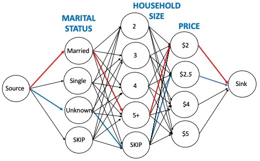
(a) Feature graph with 3 features including action (price)

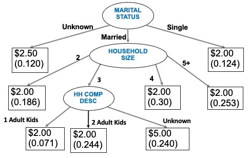
(b) A multiway-split tree with $n=8$ rules

Figure 1: A sample output from the grocery pricing use case

Decision Rule Space

The high level idea of our approach is to identify $n$ decision rules from a potentially huge rule space, which contains every possible combination of input features for policy prescription. To model this, we construct a feature graph, where each decision rule is mapped to a distinct, independent path in the graph. Specifically, we consider an acyclic multi-level digraph, $G(V,E)$, where each feature indicates a level in the graph, represented by multiple nodes corresponding to its distinct feature values. Nodes of one feature are fully connected to nodes in the next level. $V$ also contains a source and sink node. In addition, a unique and critical characteristic of $G$ is that for each feature, with the exception of the action nodes $\pi$, we introduce a dummy node SKIP. Fig 1(a) illustrates an example of a feature graph with three features, including the action nodes.

A decision rule is defined as a path $P\in\mathcal{P}$ from the source to the sink node on $G$. A path passing through a SKIP node excludes the corresponding feature from the decision rule. As SKIP nodes allow paths to ignore features, paths on this acyclic graph represent all possible feature combinations, defining the full decision rule set $\mathcal{P}$ that one has to enumerate through to solve the policy prescription problem. In the rest of the paper, we use paths and rules interchangeably.

Proposition 1

$|V|$ is linear in $d$. $|\mathcal{P}|$ is exponential in $d$.

The space for decision rules expands dramatically for high-dimensional datasets and enumerating $\mathcal{P}$ becomes intractable. We present an algorithm which searches through the space efficiently in Section An Efficient and Scalable Algorithm, by solving linear programs (LP) and dynamically generating paths when needed.

So far, we have described our approach of policy prescription as a rule selection problem, whereas the SPMT problem in (2) restricts the policy to be a multiway-split tree $\mathcal{T}_{m}(n)$. There is a key distinction between a set of decision rules and a tree: the former is viewed as unordered rules which may overlap, whereas a tree has a hierarchical structure which ensures rules are non-overlapping, i.e., each example is covered by exactly one rule (Fürnkranz 2017). In the next section, we will introduce a MIP formulation to ensure the sample-level non-overlapping condition will be satisfied by the prescribed rules. Note that while the arrangement of features in $G$ is not relevant to the objective value of (2), it does affect interpretability. Hence, we utilize insights from the teacher model and arrange the features based on their importance (e.g., Lundberg and Lee 2017) when constructing $G$ (see an example presented in the supplementary material).

Set Partitioning Problem

We now present a novel path-based MIP formulation to select a subset of $n$ rules from a feature graph. We denote decision rule as $j=1,\cdots,N$, where $N=|\mathcal{P}|$. Let $S_{j}\in[M]$ be the subset of observations which fall into rule $j$. Every sample in $S_{j}$ is prescribed with a same action $q_{j}\in\Pi$. Let $z_{j}$ be a binary decision variable which indicates whether rule $j$ is selected (1) or not (0), for $j=1,\cdots,N$. We would like to enforce that each sample $i$ is only assigned to a single rule, and failure to comply with the condition incurs a positive cost $c_{i}=c$ for all $i$. Define $r_{j}$ as the expected outcome associated with rule $j$, i.e., $r_{j}=\sum_{i\in S_{j}}g_{i,q_{j}}$. The set partitioning problem (SPP) which identifies $n$ out of $N$ decision rules can be written as follows,

$$\quad\max\quad \sum_{j=1}^{N}r_{j}z_{j}-\sum_{i=1}^{M}c_{i}s_{i}$$

s.t. $$\sum_{j=1}^{N}a_{ij}z_{j}+s_{i}=1,\quad\forall i=1,\cdots,M$$ (3)

$$\sum_{j=1}^{N}z_{j}\leq n$$ (4)

$$z_{j}\in\{1,0\},\quad\forall j=1,\cdots,N$$

$$s_{i}\geq 0,\quad\forall i=1,\cdots,M$$

where $a_{ij}=1$ if sample $i$ satisfies the conditions (features) specified in rule $j$, and 0 otherwise. While a sample may fall into several rules, the set partitioning constraint (3) along with the non-negative slack variables $s_{i}$ that are included with a sufficiently large penalty $c_{i}$, ensure that each sample is ultimately covered by exactly one rule. Cardinality constraint (4) ensures that at most $n$ rules are active in the optimal solution $\mathbf{z}^{*}$, where $n$ is a user defined input corresponding to $2^{k}$ leaf nodes in a binary-split tree of depth $k$.

Theorem 1

Active paths in $\mathcal{P}$ which are identified by $\mathbf{z}^{*}$ correspond to an optimal solution $\mathcal{T}^{*}_{m}(n)$ in SPMT.

We have shown that if we can solve SPP, then we have identified a multiway-split tree with $n$ rules. It is well-known that SPP is NP-Hard (Wolsey and Nemhauser 1999). Nevertheless, (near) optimal or high quality feasible solutions can be obtained in practice for moderate sized instances (Atamtürk, Nemhauser, and Savelsbergh 1996). Unfortunately, in our case, the cardinality of feasible rules may become prohibitive to solve it directly. We will now present an efficient algorithm to overcome this hurdle.

An Efficient and Scalable Algorithm

The technique of column generation (CG) is used for solving linear problems with a huge number of variables for which it is not practical to explicitly generate all columns (variables) of the problem matrix. More specifically, we consider a restricted master problem (RMP) version of SPP, where we 1) consider only a subset of paths, $\hat{N}$, where $\hat{N}$ is typically much smaller than $N$, and 2) relax the integrality constraints on $z_{j}$ to $0\leq z_{j}\leq 1$ for all $j=1,\cdots,\hat{N}$.

Denote the dual variables associated with the set partitioning constraints in (3) and the cardinality constraint in (4) as ${\lambda}_{i}$ and $\mu$ respectively. The dual formulation of RMP can be found in the supplementary material. In particular, the dual feasibility constraint corresponding to path $j$ is given by

$$\sum_{i=1}^{M}a_{ij}\lambda_{i}+\mu\geq r_{j},\quad\forall j=1,\cdots,\hat{N}$$ (5)

From (5), we can derive the reduced cost for path $j$ as

$$rc_{j}=r_{j}-\left(\sum_{i=1}^{M}a_{ij}\lambda_{i}+\mu\right).$$ (6)

Additional constraints are handled in (6) similar to the partitioning and cardinality restrictions via their corresponding dual variables.

The key idea of CG is as follows - as we solve a much smaller RMP to optimality, dual feasibility is guaranteed only for the rules included in $\hat{N}$ and we must verify that the dual feasibility are also satisfied by the rules not included in the RMP. A path violating the dual constraint (5) has a positive reduced cost and must be added to the RMP. Therefore, we identify paths that maximally violate Eq (5), i.e., $\max rc_{j}$ or $\min-rc_{j}$. The implicit search for $K$ paths having the highest reduced cost amounts to optimizing a subproblem, which is a K-shortest path problem (KSP) over $G$ (Horne 1980; Irnich and Desaulniers 2005), where the cost on a path is the negative of its reduced cost defined in (6). The CG procedure converges to an optimal solution of the LP relaxation of SPP when dual feasibility is achieved, i.e., $rc_{j}\leq 0$ for all $j=1,\cdots,N$. Otherwise, new paths are found and their corresponding columns $A_{j}$ which comprise of coefficients $a_{ij}$ are added to RMP, which is re-optimized. We repeatedly solve RMP and KSP until successive dual solutions converge or we reach a maximum iteration limit.

Once the CG procedure has converged, we reimpose the binary restrictions on $\mathbf{z}$ and solve the resultant Master-MIP. Any of two MIP approaches below can be adopted either individually or in combination depending on the end goal. Since SPP is NP-Hard, obtaining a provably optimal solution may require inordinate run times for challenging instances. For simplicity and replicability, we solve the Master-MIP directly here using a standard optimization library (CPLEX 2020) to distill a (near) optimal subset of prescriptive decision rules. Thereafter, one can optionally switch to the more advanced “branch-and-price” method to converge to an optimal MIP solution (Barnhart et al. 1998).

One common yet critical requirement of prescriptive analytics is to incorporate a myriad of operational constraints. They can be broadly categorized into intra-rule and inter-rule constraints, which are handled differently in the algorithm.

The scope of intra-rule constraints is limited to a single decision rule. They may involve complex path-dependent nonlinear conditions involving several features that cannot be abstracted efficiently into linear constraints. For instance, disallowing certain feature combinations or limiting the number of features. These constraints are easily handled within the KSP subproblem as a feasibility check while extending a partial path to the next node in $G$ (we refer readers to Section 1.2 in Barnhart et al. 1998 for more discussions).

Inter-rule constraints span across many decision rules. One example is the cardinality constraint in (4). Inter-rule constraints can be expressed as linear inequalities in the RMP, which in turn influence the subproblem by modifying the reduced cost. We present detailed use cases in Section Real Datasets along with a house pricing constraint and loyalty pricing implementation in the supplementary material.

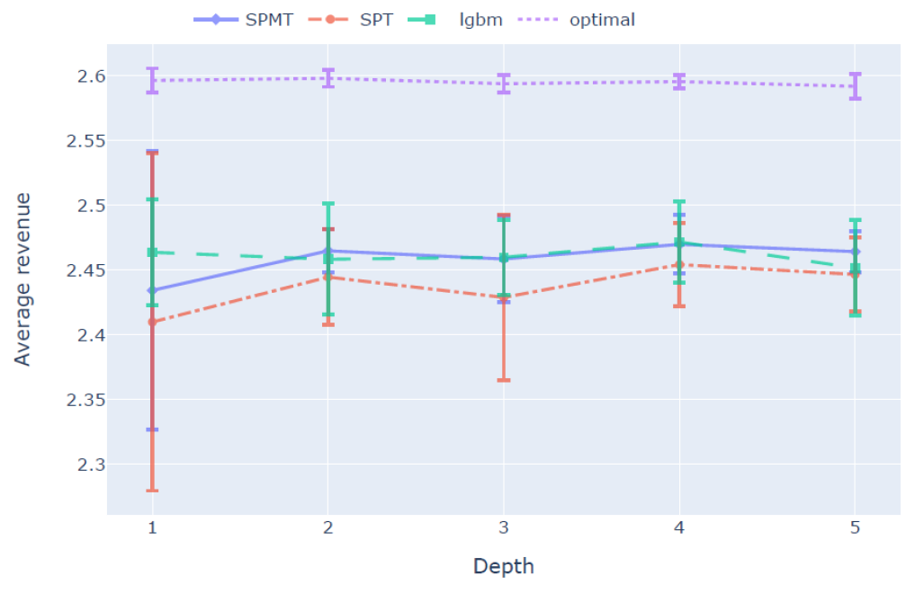
(a) Revenue with varying tree depth

(b) Revenue with varying training data size

Figure 2: Experiment results on realized outcome for synthetic Dataset (6)

Experiments

In this section, we perform experiments to demonstrate the efficacy of our method, Student Prescriptive Multiway-split Tree (SPMT). We first perform experiments on six simulated datasets which allow us to accurately calculate the resulting outcome. We want to point out that since none of the existing interpretable tree-based methods are capable of handling constraints, we can only benchmark against them in the unconstrained setting. Next, we present three use cases with real data as we discuss constrained policy prescription, two of which use publicly available data.

The following baselines are considered: The greedy student prescriptive tree (SPT), is used as the key tree-based prescriptive benchmark since Biggs, Sun, and Ettl 2021 has demonstrated that it outperforms other competing prescriptive tree methods (i.e., Kallus 2017; Athey and Imbens 2016). A true optimum policy (optimal) which can be found by identifying the price which results in the highest revenue according to the underlying probability model in synthetic datasets. The baseline (lgbm) determines the sample-level optimal policy based on the predictions of a lightGBM model, which is also the teacher model. All experiments were run on an Intel 8-core i7 PC with 32GB RAM. CPLEX 20.1 was used to solve the RMP. The minimum number of samples per rule for SPMT is set to 10. $K=100$ for KSP.

Synthetic Datasets

We follow the identical setup in Biggs, Sun, and Ettl 2021, where we generate six datasets consisting entirely of numerical features, simulated from different generative demand models. The data generation process can be found in the supplementary materials. We train a gradient boosted tree ensemble model using the lightGBM package (Ke et al. 2017) as the teacher model. The action set consists of 9 prices, ranging from the $10^{th}$ to the $90^{th}$ percentile of observed prices in $10\%$ increments.

Varying policy size We explore how the expected revenue changes with the number of policies. We use a SPT of depth $k$ which is grown to its full width to benchmark against a multiway-split tree (SPMT) with $n=2^{k}$ rules, where $k=\{1,..,5\}$. The number of training samples is held constant at $M=5000$. For each tree depth, we run 10 independent simulations for each dataset and each $k$ (i.e., 300 experiments in total). We highlight the results for $k=3$ and 5 in Table 1, which summarizes mean revenue over the simulations. Fig 2(a) shows the performance on dataset (6) with respect to the number of rules as an illustrative example, while detailed results for individual datasets are included in the supplementary materials.

Although both SPMT and SPT use the same teacher model, SPMT generally outperforms SPT, which employs a greedy heuristic, as seen in the modest gains shown in the experiments. Furthermore, SPT is unable to incorporate constraints, a shortcoming which severely limits its usefulness.

n = 8 / k = 3 n = 32 / k = 5 Dataset optimal lgbm SPMT SPT SPMT SPT 1 3.275 (0.016) 3.161 (0.054) 3.233 (0.038) 3.201 (0.071) 3.201 (0.053) 3.188 (0.063) 2 2.963 (0.034) 2.716 (0.038) 2.166 (0.034) 2.127 (0.042) 2.378 (0.015) 2.277 (0.039) 3 3.420(0.006) 3.275 (0.064) 3.347(0.048) 3.331(0.052) 3.336(0.047) 3.333(0.047) 4 3.492(0.012) 3.344 (0.057) 3.365(0.051) 3.343(0.079) 3.379(0.055) 3.366(0.06) 5 3.35(0.007) 3.260 (0.029) 3.291(0.056) 3.260(0.067) 3.296(0.017) 3.287(0.022) 6 2.592(0.01) 2.456 (0.033) 2.459(0.033) 2.429(0.064) 2.464(0.016) 2.447(0.029)

Table 1: Comparison on realized outcome for synthetic datasets ($M=5000$)

Varying data size We also investigate how SPMT performs as the size of the samples increases, where $M=\{100,300,10^{3},3\times 10^{3},10^{4},3\times 10^{4},10^{5},3\times 10^{5},6\times 10^{5},9\times 10^{5},10^{6}\}$. We focus on $n=8$ and 32 rules, again for 10 independent iterations for each configuration (i.e., 220 experiments) using Dataset (6). Fig 2(b) shows the result on realized revenue versus data size $M$.

The baseline lgbm is an upper bound to SPMT in theory since the latter trades off performance for interpretability. It can be seen as the revenue gap between lgbm and SPMT policies Fig 2(b) when the training sample size becomes large and the lgbm model produces a more accurate estimate of the underlying groundtruth. With small sample sizes, lgbm may overfit and the realized outcome may appear worse/noisier. It is crucial to note that policy from the lgbm baseline is not interpretable and can be potentially very complex (such as a fully personalized price). It is also not surprising that a policy with more rules generally outperforms fewer rules. However, once the sample size exceeds $3\times 10^{4}$, both policies with $n=8$ and $32$ converge to the same realized revenue and we do not observe further improvement from either policy by increasing the sample size.

Runtime study We investigate CG runtime as the sample size $M$ increases from 100 to $10^{6}$, with the same setup described earlier. In our experiments, all RMP instances converged in less than 20 CG iterations, with 11.19 (1.33) seconds for each iteration of RMP and KSP. Detailed results are available in the supplementary material. The key observation is that our proposed SPMT approach is inherently more scalable than prior MIP approaches when near-optimal solutions suffice. In the experiment which allowed up to 32 rules for the dataset having $10^{6}$ samples, prior MIP models would require more than $32\times 10^{6}$ binary variables. In comparison, our Master-MIP required less than 3000 binary variables.

Real Datasets

Grocery pricing case study We consider the problem of grocery pricing, using a publicly available dataset that contains over two years of household level transactions from a group of 2,500 households at a grocery retailer. A processed dataset with 97,295 rows which contain both purchases and “no-purchases” of strawberries is available online.

The unconstrained use case of maximizing expected revenue has been studied in Biggs, Sun, and Ettl 2021 and Amram, Dunn, and Zhuo 2020. We follow the same experiment setup described in these papers, where we divide the data in halves, and independently train a teacher and an evaluator (as the ground truth) using lightGBM. With $n=64$, SPMT policy achieves 82.8% increase in revenue over the historical baseline, compared to 65.9% and 77.1% reported in Biggs, Sun, and Ettl 2021 and Amram, Dunn, and Zhuo 2020 respectively. Noting that the latter work and our approach both seek optimal prescriptive policies, the difference in gain highlights the benefit of a multiway-split tree over a binary-split tree, for being more informative. An example of a SPMT with $n=8$ is shown in Fig 1(b).

There are two drawbacks with the existing unconstrained policy. First, its predicted demand almost doubles the historical sales, which may not be realizable due to supply constraints and other limitations. Second, the price discrimination based on customer-level features raises legal and fairness concerns. We briefly describe two constrained scenarios to address these issues, where more details are provided in the supplementary material. First, stores are grouped into 5 clusters based on historical sales and we require the predicted demand under a new pricing policy does not deviate too much from the historical average. With $n=64$, SPMT produces rules that result in 47.49% and 61.72% increase in revenue when the allowable change in predicted demand is set to 25% and 50% of the historical value. In a separate scenario, we use inter-rule constraints to model a store-based loyalty pricing policy, where all shoppers at a store receive the same price except loyalty-card shoppers, who receive a price that is same or lower. This setting is an example of inter-rule constraints involving logical conjunctions of categorical and numerical features (StoreID, Loyalty, Price), which are handled naturally in our path-based MIP, but relatively difficult to express efficiently using arc-based feature-level models. The resulting pricing policy using only storeID and a loyalty indicator to define rules achieves 65.4% increase in revenue over the baseline without discriminating customers based on their personal features.

Housing upgrade use case We consider a Kaggle dataset on house prices that includes numerical and categorical attributes such as age, square footage, number of bedrooms, bathrooms, zipcode, as well as grade, i.e., an index from 1-13, where higher value indicates better construction and design. We first train a regression model to predict the house value given the attributes as the teacher. We then formulate a prescriptive problem, i.e., maximize the predicted sale price in the test set by adjusting the grade of individual houses. As the teacher model predicts that grade increases the house value, an unconstrained policy search simply recommends that all houses upgrade to the highest level.

One of the constrained scenarios that we consider requires houses to “conform to the neighborhood”, i.e., the predicted sale price of houses with the same zip code must be within 10% of the historical value. The decision rules no longer upgrade all houses but prescribe a mix of upgrades and downgrades based on other housing features while satisfying the price constraint for each neighborhood. More constrained scenarios are included in the supplementary materials.

Airline pricing use case We consider the task of pricing premium seats for a large airline (an industry partner) using easily interpretable prescriptive rules. The dataset contains more than 1.3 million samples across multiple markets with several features such as departure day and time, duration of the flight, market, whether one-way or round trip. We want to point out that our work allows multiple actions to be added as stacks of action nodes e.g., to represent the prices for the first class, business class and premium economy seats respectively. Structured decision making can be modeled as constraints, e.g., given the same trip information, a business class (premium economy) seat should be at least $250 cheaper than a first (business) class seat. For confidentiality reasons, details of the study are omitted.

We compare the policies from the greedy SPT and our proposed SPMT method for a same number of decision rules. With SPT, seat capacity limits were violated and resulted in a overly high predicted gain. Further analysis revealed that these rules would have allowed early bookers to purchase premium seats at a bargain, cannibalizing the demand from high-value customers who typically show up later. By adding market-specific capacity constraints on the predicted conversions, we revised the rules to achieve a more realistic gain that is more likely to be realized in live settings.

Conclusion

Our work adds to a stream of growing research which deserves more attention in the literature due to its paramount practical importance, i.e., generating interpretable policy from data for decision making. We address the problem of distilling prescriptive rules using a teacher model, providing counterfactual estimates. We formulate a mixed integer optimization problem to distill active decision rules that are shown to represent a multiway-split tree on an acyclic feature graph. The number of binary decision variables in our model can increase exponentially in the number of features that comprise the rules. As only a small subset of rules are active in an optimal solution, we propose a column generation approach to solve the MIP. Our method can handle complex inter-rule and intra-rule constraints that cannot be satisfied by existing prescriptive tree methods. We provide computational results on synthetic and publicly available real-life data and solve instances having up to a million samples within an hour of computation time. The proposed method offers a generic and widely applicable way of generating (near) optimal prescriptive rules by transforming blackbox AI/ML predictions into operationally effective decisions that may benefit enterprises.

References

- Aghaei, Azizi, and Vayanos (2019) Aghaei, S.; Azizi, M. J.; and Vayanos, P. 2019. Learning optimal and fair decision trees for non-discriminative decision-making. In Proceedings of the AAAI Conference on Artificial Intelligence, volume 33, 1418–1426.
- Aghaei, Gomez, and Vayanos (2020) Aghaei, S.; Gomez, A.; and Vayanos, P. 2020. Learning optimal classification trees: Strong max-flow formulations. arXiv preprint arXiv:2002.09142.
- Amram, Dunn, and Zhuo (2020) Amram, M.; Dunn, J.; and Zhuo, Y. D. 2020. Optimal Policy Trees. arXiv preprint arXiv:2012.02279.
- Atamtürk, Nemhauser, and Savelsbergh (1996) Atamtürk, A.; Nemhauser, G. L.; and Savelsbergh, M. W. 1996. A combined Lagrangian, linear programming, and implication heuristic for large-scale set partitioning problems. Journal of heuristics, 1(2): 247–259.
- Athey and Imbens (2016) Athey, S.; and Imbens, G. 2016. Recursive partitioning for heterogeneous causal effects. Proceedings of the National Academy of Sciences, 113(27): 7353–7360.
- Bach (2008) Bach, F. 2008. Exploring large feature spaces with hierarchical multiple kernel learning. arXiv preprint arXiv:0809.1493.
- Barnhart et al. (1998) Barnhart, C.; Johnson, E. L.; Nemhauser, G. L.; Savelsbergh, M. W.; and Vance, P. H. 1998. Branch-and-price: Column generation for solving huge integer programs. Operations research, 46(3): 316–329.
- Bertsimas and Dunn (2017) Bertsimas, D.; and Dunn, J. 2017. Optimal classification trees. Machine Learning, 106(7): 1039–1082.
- Bertsimas, Dunn, and Mundru (2019) Bertsimas, D.; Dunn, J.; and Mundru, N. 2019. Optimal prescriptive trees. INFORMS Journal on Optimization, 1(2): 164–183.
- Biggs, Sun, and Ettl (2021) Biggs, M.; Sun, W.; and Ettl, M. 2021. Model Distillation for Revenue Optimization: Interpretable Personalized Pricing. In International Conference on Machine Learning, 946–956. PMLR.
- Breiman et al. (1984) Breiman, L.; Friedman, J.; Stone, C. J.; and Olshen, R. A. 1984. Classification and regression trees. CRC press.
- Bront, Méndez-Díaz, and Vulcano (2009) Bront, J. J. M.; Méndez-Díaz, I.; and Vulcano, G. 2009. A column generation algorithm for choice-based network revenue management. Operations research, 57(3): 769–784.
- Carvalho, Pereira, and Cardoso (2019) Carvalho, D. V.; Pereira, E. M.; and Cardoso, J. S. 2019. Machine learning interpretability: A survey on methods and metrics. Electronics, 8(8): 832.
- Chen and Xu (2006) Chen, Z.-L.; and Xu, H. 2006. Dynamic column generation for dynamic vehicle routing with time windows. Transportation Science, 40(1): 74–88.
- CPLEX (2020) CPLEX, I. 2020. Introducing IBM ILOG CPLEX Optimization Studio 20.1.0. https://www.ibm.com/docs/en/icos/20.1.0. Accessed: 2021-03-25.
- Desaulniers, Desrosiers, and Solomon (2006) Desaulniers, G.; Desrosiers, J.; and Solomon, M. M. 2006. Column generation, volume 5. Springer Science & Business Media.
- Dudík, Langford, and Li (2011) Dudík, M.; Langford, J.; and Li, L. 2011. Doubly Robust Policy Evaluation and Learning. In ICML.
- Ford Jr and Fulkerson (1958) Ford Jr, L. R.; and Fulkerson, D. R. 1958. A suggested computation for maximal multi-commodity network flows. Management Science, 5(1): 97–101.
- Frosst and Hinton (2017) Frosst, N.; and Hinton, G. 2017. Distilling a neural network into a soft decision tree. arXiv preprint arXiv:1711.09784.
- Fulton, Kasif, and Salzberg (1995) Fulton, T.; Kasif, S.; and Salzberg, S. 1995. Efficient algorithms for finding multi-way splits for decision trees. In Machine Learning Proceedings 1995, 244–251. Elsevier.
- Fürnkranz (2017) Fürnkranz, J. 2017. Decision Lists and Decision Trees, 328–329.
- Guidotti et al. (2018) Guidotti, R.; Monreale, A.; Ruggieri, S.; Turini, F.; Giannotti, F.; and Pedreschi, D. 2018. A survey of methods for explaining black box models. ACM computing surveys (CSUR), 51(5): 1–42.
- Hinton, Vinyals, and Dean (2015) Hinton, G.; Vinyals, O.; and Dean, J. 2015. Distilling the knowledge in a neural network. arXiv preprint arXiv:1503.02531.
- Hirano and Imbens (2004) Hirano, K.; and Imbens, G. W. 2004. The propensity score with continuous treatments. Applied Bayesian modeling and causal inference from incomplete-data perspectives, 226164: 73–84.
- Horne (1980) Horne, G. 1980. Finding the K least cost paths in an acyclic activity network. Journal of the Operational Research Society, 31(5): 443–448.
- Irnich and Desaulniers (2005) Irnich, S.; and Desaulniers, G. 2005. Shortest path problems with resource constraints. In Column generation, 33–65. Springer.
- Jawanpuria, Nath, and Ramakrishnan (2011) Jawanpuria, P.; Nath, J. S.; and Ramakrishnan, G. 2011. Efficient rule ensemble learning using hierarchical kernels. In ICML.
- Kallus (2017) Kallus, N. 2017. Recursive partitioning for personalization using observational data. In Proceedings of the 34th International Conference on Machine Learning-Volume 70, 1789–1798. JMLR. org.
- Ke et al. (2017) Ke, G.; Meng, Q.; Finley, T.; Wang, T.; Chen, W.; Ma, W.; Ye, Q.; and Liu, T.-Y. 2017. Lightgbm: A highly efficient gradient boosting decision tree. In Advances in neural information processing systems, 3146–3154.
- Klabjan et al. (2002) Klabjan, D.; Johnson, E. L.; Nemhauser, G. L.; Gelman, E.; and Ramaswamy, S. 2002. Airline crew scheduling with time windows and plane-count constraints. Transportation science, 36(3): 337–348.
- Künzel et al. (2019) Künzel, S. R.; Sekhon, J. S.; Bickel, P. J.; and Yu, B. 2019. Metalearners for estimating heterogeneous treatment effects using machine learning. Proceedings of the national academy of sciences, 116(10): 4156–4165.
- Laurent and Rivest (1976) Laurent, H.; and Rivest, R. L. 1976. Constructing optimal binary decision trees is NP-complete. Information processing letters, 5(1): 15–17.
- Lepenioti et al. (2020) Lepenioti, K.; Bousdekis, A.; Apostolou, D.; and Mentzas, G. 2020. Prescriptive analytics: Literature review and research challenges. International Journal of Information Management, 50: 57–70.
- Liu et al. (2018) Liu, G.; Schulte, O.; Zhu, W.; and Li, Q. 2018. Toward interpretable deep reinforcement learning with linear model u-trees. In Joint European Conference on Machine Learning and Knowledge Discovery in Databases, 414–429. Springer.
- Lundberg and Lee (2017) Lundberg, S. M.; and Lee, S.-I. 2017. A unified approach to interpreting model predictions. In Advances in neural information processing systems, 4765–4774.
- Miller (2019) Miller, T. 2019. Explanation in artificial intelligence: Insights from the social sciences. Artificial intelligence, 267: 1–38.
- Puiutta and Veith (2020) Puiutta, E.; and Veith, E. M. 2020. Explainable reinforcement learning: A survey. In International Cross-Domain Conference for Machine Learning and Knowledge Extraction, 77–95. Springer.
- Ribeiro, Singh, and Guestrin (2016) Ribeiro, M. T.; Singh, S.; and Guestrin, C. 2016. ” Why should i trust you?” Explaining the predictions of any classifier. In Proceedings of the 22nd ACM SIGKDD international conference on knowledge discovery and data mining, 1135–1144.
- Shalit, Johansson, and Sontag (2017) Shalit, U.; Johansson, F. D.; and Sontag, D. 2017. Estimating individual treatment effect: generalization bounds and algorithms. In International Conference on Machine Learning, 3076–3085. PMLR.
- Subramanian and Sherali (2008) Subramanian, S.; and Sherali, H. D. 2008. An effective deflected subgradient optimization scheme for implementing column generation for large-scale airline crew scheduling problems. INFORMS Journal on Computing, 20(4): 565–578.
- Wager and Athey (2018) Wager, S.; and Athey, S. 2018. Estimation and inference of heterogeneous treatment effects using random forests. Journal of the American Statistical Association, 113(523): 1228–1242.
- Wolsey and Nemhauser (1999) Wolsey, L. A.; and Nemhauser, G. L. 1999. Integer and combinatorial optimization, volume 55. John Wiley & Sons.
- Xu (2019) Xu, Y. 2019. Solving Large Scale Optimization Problems in the Transportation Industry and Beyond Through Column Generation. In Optimization in Large Scale Problems, 269–292. Springer.
- Zhou, Athey, and Wager (2018) Zhou, Z.; Athey, S.; and Wager, S. 2018. Offline multi-action policy learning: Generalization and optimization. arXiv preprint arXiv:1810.04778.
- Zhu et al. (2020) Zhu, H.; Murali, P.; Phan, D.; Nguyen, L.; and Kalagnanam, J. 2020. A Scalable MIP-based Method for Learning Optimal Multivariate Decision Trees. In Advances in Neural Information Processing Systems, volume 33, 1771–1781.
- Aghaei, Azizi, and Vayanos [2019] Aghaei, S.; Azizi, M. J.; and Vayanos, P. 2019. Learning optimal and fair decision trees for non-discriminative decision-making. In Proceedings of the AAAI Conference on Artificial Intelligence, volume 33, 1418–1426.
- Aghaei, Gomez, and Vayanos [2020] Aghaei, S.; Gomez, A.; and Vayanos, P. 2020. Learning optimal classification trees: Strong max-flow formulations. arXiv preprint arXiv:2002.09142.
- Amram, Dunn, and Zhuo [2020] Amram, M.; Dunn, J.; and Zhuo, Y. D. 2020. Optimal Policy Trees. arXiv preprint arXiv:2012.02279.
- Atamtürk, Nemhauser, and Savelsbergh [1996] Atamtürk, A.; Nemhauser, G. L.; and Savelsbergh, M. W. 1996. A combined Lagrangian, linear programming, and implication heuristic for large-scale set partitioning problems. Journal of heuristics, 1(2): 247–259.
- Athey and Imbens [2016] Athey, S.; and Imbens, G. 2016. Recursive partitioning for heterogeneous causal effects. Proceedings of the National Academy of Sciences, 113(27): 7353–7360.
- Bach [2008] Bach, F. 2008. Exploring large feature spaces with hierarchical multiple kernel learning. arXiv preprint arXiv:0809.1493.
- Barnhart et al. [1998] Barnhart, C.; Johnson, E. L.; Nemhauser, G. L.; Savelsbergh, M. W.; and Vance, P. H. 1998. Branch-and-price: Column generation for solving huge integer programs. Operations research, 46(3): 316–329.
- Bertsimas and Dunn [2017] Bertsimas, D.; and Dunn, J. 2017. Optimal classification trees. Machine Learning, 106(7): 1039–1082.
- Bertsimas, Dunn, and Mundru [2019] Bertsimas, D.; Dunn, J.; and Mundru, N. 2019. Optimal prescriptive trees. INFORMS Journal on Optimization, 1(2): 164–183.
- Biggs, Sun, and Ettl [2021] Biggs, M.; Sun, W.; and Ettl, M. 2021. Model Distillation for Revenue Optimization: Interpretable Personalized Pricing. In International Conference on Machine Learning, 946–956. PMLR.
- Breiman et al. [1984] Breiman, L.; Friedman, J.; Stone, C. J.; and Olshen, R. A. 1984. Classification and regression trees. CRC press.
- Bront, Méndez-Díaz, and Vulcano [2009] Bront, J. J. M.; Méndez-Díaz, I.; and Vulcano, G. 2009. A column generation algorithm for choice-based network revenue management. Operations research, 57(3): 769–784.
- Carvalho, Pereira, and Cardoso [2019] Carvalho, D. V.; Pereira, E. M.; and Cardoso, J. S. 2019. Machine learning interpretability: A survey on methods and metrics. Electronics, 8(8): 832.
- Chen and Xu [2006] Chen, Z.-L.; and Xu, H. 2006. Dynamic column generation for dynamic vehicle routing with time windows. Transportation Science, 40(1): 74–88.
- CPLEX [2020] CPLEX, I. 2020. Introducing IBM ILOG CPLEX Optimization Studio 20.1.0. https://www.ibm.com/docs/en/icos/20.1.0. Accessed: 2021-03-25.
- Desaulniers, Desrosiers, and Solomon [2006] Desaulniers, G.; Desrosiers, J.; and Solomon, M. M. 2006. Column generation, volume 5. Springer Science & Business Media.
- Dudík, Langford, and Li [2011] Dudík, M.; Langford, J.; and Li, L. 2011. Doubly Robust Policy Evaluation and Learning. In ICML.
- Ford Jr and Fulkerson [1958] Ford Jr, L. R.; and Fulkerson, D. R. 1958. A suggested computation for maximal multi-commodity network flows. Management Science, 5(1): 97–101.
- Frosst and Hinton [2017] Frosst, N.; and Hinton, G. 2017. Distilling a neural network into a soft decision tree. arXiv preprint arXiv:1711.09784.
- Fulton, Kasif, and Salzberg [1995] Fulton, T.; Kasif, S.; and Salzberg, S. 1995. Efficient algorithms for finding multi-way splits for decision trees. In Machine Learning Proceedings 1995, 244–251. Elsevier.
- Fürnkranz [2017] Fürnkranz, J. 2017. Decision Lists and Decision Trees, 328–329.
- Guidotti et al. [2018] Guidotti, R.; Monreale, A.; Ruggieri, S.; Turini, F.; Giannotti, F.; and Pedreschi, D. 2018. A survey of methods for explaining black box models. ACM computing surveys (CSUR), 51(5): 1–42.
- Hinton, Vinyals, and Dean [2015] Hinton, G.; Vinyals, O.; and Dean, J. 2015. Distilling the knowledge in a neural network. arXiv preprint arXiv:1503.02531.
- Hirano and Imbens [2004] Hirano, K.; and Imbens, G. W. 2004. The propensity score with continuous treatments. Applied Bayesian modeling and causal inference from incomplete-data perspectives, 226164: 73–84.
- Horne [1980] Horne, G. 1980. Finding the K least cost paths in an acyclic activity network. Journal of the Operational Research Society, 31(5): 443–448.
- Irnich and Desaulniers [2005] Irnich, S.; and Desaulniers, G. 2005. Shortest path problems with resource constraints. In Column generation, 33–65. Springer.
- Jawanpuria, Nath, and Ramakrishnan [2011] Jawanpuria, P.; Nath, J. S.; and Ramakrishnan, G. 2011. Efficient rule ensemble learning using hierarchical kernels. In ICML.
- Kallus [2017] Kallus, N. 2017. Recursive partitioning for personalization using observational data. In Proceedings of the 34th International Conference on Machine Learning-Volume 70, 1789–1798. JMLR. org.
- Ke et al. [2017] Ke, G.; Meng, Q.; Finley, T.; Wang, T.; Chen, W.; Ma, W.; Ye, Q.; and Liu, T.-Y. 2017. Lightgbm: A highly efficient gradient boosting decision tree. In Advances in neural information processing systems, 3146–3154.
- Klabjan et al. [2002] Klabjan, D.; Johnson, E. L.; Nemhauser, G. L.; Gelman, E.; and Ramaswamy, S. 2002. Airline crew scheduling with time windows and plane-count constraints. Transportation science, 36(3): 337–348.
- Künzel et al. [2019] Künzel, S. R.; Sekhon, J. S.; Bickel, P. J.; and Yu, B. 2019. Metalearners for estimating heterogeneous treatment effects using machine learning. Proceedings of the national academy of sciences, 116(10): 4156–4165.
- Laurent and Rivest [1976] Laurent, H.; and Rivest, R. L. 1976. Constructing optimal binary decision trees is NP-complete. Information processing letters, 5(1): 15–17.
- Lepenioti et al. [2020] Lepenioti, K.; Bousdekis, A.; Apostolou, D.; and Mentzas, G. 2020. Prescriptive analytics: Literature review and research challenges. International Journal of Information Management, 50: 57–70.
- Liu et al. [2018] Liu, G.; Schulte, O.; Zhu, W.; and Li, Q. 2018. Toward interpretable deep reinforcement learning with linear model u-trees. In Joint European Conference on Machine Learning and Knowledge Discovery in Databases, 414–429. Springer.
- Lundberg and Lee [2017] Lundberg, S. M.; and Lee, S.-I. 2017. A unified approach to interpreting model predictions. In Advances in neural information processing systems, 4765–4774.
- Miller [2019] Miller, T. 2019. Explanation in artificial intelligence: Insights from the social sciences. Artificial intelligence, 267: 1–38.
- Puiutta and Veith [2020] Puiutta, E.; and Veith, E. M. 2020. Explainable reinforcement learning: A survey. In International Cross-Domain Conference for Machine Learning and Knowledge Extraction, 77–95. Springer.
- Ribeiro, Singh, and Guestrin [2016] Ribeiro, M. T.; Singh, S.; and Guestrin, C. 2016. ” Why should i trust you?” Explaining the predictions of any classifier. In Proceedings of the 22nd ACM SIGKDD international conference on knowledge discovery and data mining, 1135–1144.
- Shalit, Johansson, and Sontag [2017] Shalit, U.; Johansson, F. D.; and Sontag, D. 2017. Estimating individual treatment effect: generalization bounds and algorithms. In International Conference on Machine Learning, 3076–3085. PMLR.
- Subramanian and Sherali [2008] Subramanian, S.; and Sherali, H. D. 2008. An effective deflected subgradient optimization scheme for implementing column generation for large-scale airline crew scheduling problems. INFORMS Journal on Computing, 20(4): 565–578.
- Wager and Athey [2018] Wager, S.; and Athey, S. 2018. Estimation and inference of heterogeneous treatment effects using random forests. Journal of the American Statistical Association, 113(523): 1228–1242.
- Wolsey and Nemhauser [1999] Wolsey, L. A.; and Nemhauser, G. L. 1999. Integer and combinatorial optimization, volume 55. John Wiley & Sons.
- Xu [2019] Xu, Y. 2019. Solving Large Scale Optimization Problems in the Transportation Industry and Beyond Through Column Generation. In Optimization in Large Scale Problems, 269–292. Springer.
- Zhou, Athey, and Wager [2018] Zhou, Z.; Athey, S.; and Wager, S. 2018. Offline multi-action policy learning: Generalization and optimization. arXiv preprint arXiv:1810.04778.
- Zhu et al. [2020] Zhu, H.; Murali, P.; Phan, D.; Nguyen, L.; and Kalagnanam, J. 2020. A Scalable MIP-based Method for Learning Optimal Multivariate Decision Trees. In Advances in Neural Information Processing Systems, volume 33, 1771–1781.