Dot Product Bounds in Galois Rings

ABSTRACT

We consider a problem related to the Erdős Unit Distance Conjecture: How often can a single dot product configuration or a multiple dot product configuration occur over a Galoi Ring? We also find a bound on an inverse vector matrix multiplication problem.

KEYWORDS: Dot Product, Erdős Unit Distance Conjecture, Galois Rings

1 Introduction

In 1946, Paul Erdős asked how many unit distances may occur in the plane with $n$ points? Erdős proved that $n$ points in $R^{2}$ determines $\Omega(n^{1/2})$ many unit distances and conjectured that there are $\Omega(n^{c})$ for any $c<1$ (see [7]). The best known result is $\Omega(n/\log(n))$ by Guth and Katz [9] in 2015. For $R^{d}$, Erdős proved that $n$ points determines $\Theta(n^{2/d})$ unit distances and in 2008 Solymosi and Vu proved the bound of $\Omega(n^{2/d-2/(d(d+2))})$ [15]. The idea of the unit distance problem has since been extended to various rings by using a distance like functional. We see this in Covert, Iosevich and Pakianathan’s 2011 work [4] where they study integers modulo a prime power and also Iosevich and Rudnev’s 2008 work [12] over finite fields.

A common extension to this question is the single dot product problem: “How often can a specified dot product occur between $n$ points in some ambient space?”. This has been studied in [10], [1], [5], and more, where different bounds and configurations are studied.

1.1 Focus of the article

This article will focus on various configurations of the dot product problem in the ambient space of Galois rings. Galois rings are a set of finite rings that contain both all of $F_{p^{l}}$ and $\mathbb{Z}_{p^{l}}$. They are constructed as $R_{e,k}\cong\mathbb{Z}_{p^{e}}[x]/(f)$ where $f$ is of degree $k$ and irreducible in $\mathbb{Z}_{p}[x]$ under the mod $p$ map. The configurations that we consider are single dot products, pairs of dot products, and general forest configurations. We further show an application of the forest configuration leads to a bound on the number of solutions to the matrix equation $aA=b$ where $b$ is a given column and $a$ and $A$ are our variables.

Galois rings are finding applications in computer networking through coding theory. For more on Galois rings in coding theory see [2, §8.1.3]. Another reason to study finite rings is that they provide a test bed for complicated analysis problems as integrals are always convergent. The prototypical example of this is Zeev Dvir’s paper “On the size of Kakeya sets in finite fields” [6, Theorem 2], where he proved the Kakeya Conjecture (relates to subsets of $\mathbb{F}_{p^{l}}$ that contain a line in every direction) via simple means. We study forest configurations as they encompass all dot product configurations that contain no cycles.

1.2 Results

Our first result follows in form the proof by Covert, Iosevich, and Pakianathan [4, Theorem 1.3.2]. There they study the Erdős distance problem over the integers modulo an odd prime to a power. We define our counting function $\nu$, which counts how many pairs of points give a specified dot product.

Definition 1.

Let $E\subset R_{e,k}^{d}$. Let $p,e,k,d$ be given natural numbers with $p$ prime, $e\geq 5$, $d\geq 2$, and $k\geq 1$. Define

$$\nu(t)=\left|\{(x,y)\in E\times E:x\cdot y=t\}\right|.$$

Covert et al. in [4] show that $\nu(t)=|E|^{2}/p^{l}+R(t)$, where

$$|R(t)|<l|E|p^{l\left(\frac{d-1}{2}(2-1/l)\right)}<|E|^{2}/{p^{l}}$$

whenever $|E|>lp^{ld-d/2+1/2}$.

Our first result gives that the number of pairs of points that give a specified dot product must be no more than twice the expected value whenever the size of our point set is large enough.

Theorem 1.1.

Let $E\subset R_{e,k}^{d}$. Let $p,e,k,d$ be given natural numbers with $p$ prime, $e\geq 5$, $d\geq 2$, and $k\geq 1$. Let $\nu(t)=|\{(x,y)\in E\times E:x\cdot y=t\}|$. Then

$$\nu(t)\leq 2|E|/p^{ek}$$

for any $t\in R_{e,k}$ whenever $|E|\geq\sqrt{6+3e}p^{dek-dk/2+ek/2+k/2}$.

As $|E|\leq|R^{d}|=p^{dek}$, this result is non-trivial when $d\geq e+1+\frac{\log_{p}(6+3e)}{k}$. Our second results gives that the number of triplets of points $(x,y,z)$ that give specified dot products ($x\cdot y=\alpha,\,y\cdot z=\beta$) must be no more than twice the expected value whenever the size of our point set is large enough. Graphically, this is given in Figure 1. We define a new counting function to count these triplets of points.

Figure 1: Pair of Dot Products

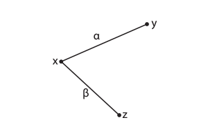
Definition 2.

Let $d\geq 3,\ e\geq 5,\ k\geq 1$. Let $E\subset(R_{e,k})^{d}$ and suppose that $\alpha,\beta\in R_{e,k}$. We define

$$\Pi_{\alpha,\beta}(E)=\{(x,y,z)\in E^{3}:x\cdot y=\alpha,x\cdot z=\beta\}.$$

The proof follows and extends the paper “Pairs of Dot Products in Finite Fields and Rings” by David Covert and Steven Senger [5], where they consider both $\mathbb{F}_{p^{l}}$ and $\mathbb{Z}_{p^{l}}$. Covert and Senger find

$$\left|\Pi_{\alpha,\beta}(E)\right|=\frac{|E|^{3}}{p^{2l}}(1+o(1))$$

whenever $|E|>cp^{l\left(\frac{d+1}{2}\right)}$ for $E\subset\mathbb{F}_{p^{l}}^{d}$ and $|E|>cp^{dl-d/2+1}$ when $E\subset\mathbb{Z}_{p^{l}}^{d}$ for some constant $c$.

Theorem 1.2.

Let $E\subset R_{e,k}^{d}$. Let $d\geq 3,\ e\geq 5,\ k\geq 1$. Let $E\subset(R_{e,k})^{d}$ and suppose that $\alpha,\beta\in R_{e,k}$. We have the bound

$$|\Pi_{\alpha,\beta}(E)|\leq\frac{2|E^{3}|}{p^{2ek}}$$

whenever $|E|\geq\sqrt{35e/8}p^{dek-dk/2+ek/2+k/2}.$

This result is non-trivial when $d\geq e+1+\log_{p}(35e/8)/k$. Our third result is similar, but for tree configurations. We extend the results of [3] by Blevins, Lynch, Senger, and the author from chains over $\mathbb{Z}_{p}^{l}$ and $\mathbb{F}_{p}^{l}$ to forests over Galois rings. We create a third counting function as follows:

Definition 3.

Let $E\subset R_{e,k}^{d}$. Let $T$ be a forest with vertices $V$ with $|V|=m$ where each vertex represents an element of $E$ and edges $\mathcal{F}$ with $|\mathcal{F}|=n$ where each edge $(e_{i},e_{j})$ represents that we have specified $e_{i}\cdot e_{j}=\alpha_{ij}$ where $\alpha=\{\alpha_{\epsilon}\}_{\epsilon\in\mathcal{F}}$ is given. An example graph is visualized in Figure 2. We define $\Pi_{\alpha}(T)=\{x\in E^{m}:\forall\alpha_{ij}\in\alpha,x_{i}\cdot x_{j}=\alpha_{ij}\}.$

Figure 2: Forest of elements and dot products

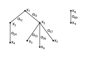
Theorem 1.1.

Let $d\geq 3,\ e\geq 5,\ k\geq 1,\ n\geq 3$. Let $E\subset R_{e,k}^{d}$. Let $T$ be a forest with vertices $V$ with $|V|=m$ where each vertex represents an element of $E$ and edges $\mathcal{F}$ with $|\mathcal{F}|=n$ where each edge $(e_{i},e_{j})$ represents that we have specified $e_{i}\cdot e_{j}=\alpha_{ij}$ where $\alpha=\{\alpha_{\epsilon}\}_{\epsilon\in\mathcal{F}}$ is given. Then

$$\Pi_{\alpha}(T)\leq\frac{2|E|^{m}}{p^{nek}}$$

whenever $|E|\geq\max\left\{2n\sqrt{6+3e}p^{dek-dk/2+3ek/2+k/2},\sqrt{14}ep^{dek-dk/2+nek/2+n/2-ek/2+k/2}\right\}.$

When $n\geq 4$, the bound on $|E|$ reduces to $|E|\geq\sqrt{14}enp^{dek-dk/2+nek/2+n/2-ek/2+3k/2}.$ This is nontrivial (with $n\geq 4$) when $d\geq(n-1)e+3+\frac{n+\log_{p}(14en^{2})}{k}$. An application of Theorem 1.1 gives a bound on how many pairs of row-vectors and matrices there are that multiply to a specified column-vector.

Theorem 1.2.

Let $d\geq 3,\ e\geq 5,\ k\geq 1,\ n\geq 4$. Let $E\subset R_{e,k}^{d}$. Let $aA=b$ be an equation where $a\in E$, the columns of $A$ are in $E$, and $b$ is a given row-vector of length $n$. Whenever $|E|>en\sqrt{14}p^{dek-dk/2+nek/2+n/2-ek/2+k}$, the number of solutions

$$S=\left|\left\{(a,A)\mid a\in E,A\in E^{n},\ aA=b\right\}\right|$$

has $S\leq\frac{2|E|^{n+1}}{p^{nek}}.$

We now compare this bound to the known number for when $e=k=1$ and $E=R^{d}_{e,k}=\mathbb{Z}_{p}^{d}$. From Hodges 1966 work [16], where he gives an expression for the number of represntations of a bilinear form ($\bmod\ p^{a}$), we are able to find that the number of such solutions $S$ is $p^{dn-n}(p^{d}-1)$ which is less than twice the expected value of $\frac{2p^{dn+d}}{p^{n}}$. The proof for Theorem 1.2 works by showing a similarity of structures. So should there be a bound on the matrix-matrix multiplication problem $AB=C$, then its bound should give a bound on a corresponding dot product configuration with cycles.

1.3 Background

For proofs of the below statements see [2], [11], and [13].

Definition 4 ($\chi_{e,k}$).

The canonical additive character $\chi_{e,k}:R_{e,k}\rightarrow\mathbf{C}^{\times}$ is defined as

$$\chi_{e,k}(z)=e^{2\pi i\operatorname{Tr}_{e,k}(z)/p^{e}}.$$

Lemma 5 (Orthogonality).

Let $e,k$ be given. For any $a\in R$,

$$\sum_{z\in R}\chi(az)=\begin{cases}|R|,&a=0\\ 0,&a\neq 0\end{cases}$$

Theorem 1.3.

Let $\beta$ be a generator of the subgroup of $R_{e,k}^{\times}$ isomorphic to $\mathbb{Z}_{p^{k}-1}$. Let $T_{e,k}=\{0,1,\beta,\ldots,\beta^{p^{k}-2}\}$. Every $z\in R$ has a unique $p$-adic representation

$$z=z_{0}+pz_{1}+\cdots+p^{e-1}z_{e-1},\quad z_{i}\in T_{e,k}.$$

Definition 6.

We will use the notation $[p^{i}]$ to mean $(p^{i})\setminus(p^{i+1})$.

Lemma 7.

Any $s\in[p^{i}]$ has the form $s=p^{i}u$ where $u$ is the uniquely determined unit of the form $u_{1}+pu_{2}+\cdots+p^{e-i-1}u_{e-i-1}$ where $u_{i}\in T_{e,k}$.

Corollary 8.

If $a\in R_{e,k}$ is given, then

$$\sum_{z\in p^{i}R_{e,k}}\chi_{e,k}(az)=\sum_{w\in R_{e-i,k}}\chi_{e-i,k}(\rho_{i}(a)w).$$

Where $\rho_{i}(a_{0}+pa_{1}+\cdots+p^{e-1}a_{e-1})=a_{0}+pa_{1}+\cdots+p^{e-1-i}a_{e-1-i}$ with $a_{0}+pa_{1}+\cdots+p^{e-1}a_{e-1}$ being the $p$-adic expansion of $a$.

Proof.

By definition of $\chi_{e,k}$, $\operatorname{Tr}$, and characteristic of a ring, this is immediate. Let $(az)_{0}+\cdots+p^{e-1}(az)_{e-1}$ be the $p$-adic expansion of $az$. Note,

$$\sum_{z\in p^{i}R_{e,k}}\chi_{e,k}(az)$$

$$=\sum_{z\in R_{e,k}}\exp\left(2\pi i\left[p^{i}az+\left(p^{i}(az)_{0}^{p}+\cdots+p^{e-1+i}(az)^{p}_{e-1}\right)+\cdots+\left(p^{i}(az)_{0}^{p^{k}}+\ldots p^{e-1+i}(az)^{p^{k}}_{e-1}\right)\right]/p^{e}\right)$$

$$=\sum_{z\in R_{e,k}}\exp\left(2\pi i\left[az+\left(p^{i}(az)_{0}^{p}+\cdots+p^{e-1-i}(az)^{p}_{e-1}\right)+\cdots+\left((az)_{0}^{p^{k}}+\cdots+p^{e-1}(az)^{p^{k}}_{e-1}\right)\right]/p^{e-i}\right)$$

$$=\sum_{w\in R_{e-i,k}}\chi_{e-i,k}(\rho_{i}(a)w).$$

∎

Lemma 9.

Let $e,k$ be given and $R=R_{e,k}$. If $n$ is a given natural number and $0<n<e$, then

$$\sum_{z\in R^{\times}}\chi(p^{n}z)\leq 0.$$

Proof.

Note that

$$\sum_{z\in R^{\times}}\chi(p^{n}z) =\sum_{z\in R}\chi(p^{n}z)-\sum_{z\in(p)}\chi(p^{n}z)$$

$$=I+II.$$

By orthogonality (Lemma 5), $I=0$. So $\sum_{z\in R^{\times}}\chi(p^{n}z)=-\sum_{z\in(p)}\chi(p^{n}z)$. Thus, when $n+1=e$, $\sum_{z\in R^{\times}}\chi(p^{n}z)=-|(p)|=-|pR_{e,k}|$. In the case that $n+1\neq e$, we apply Corollary 8,

$$\sum_{z\in R^{\times}}\chi(p^{n}z) =-\sum_{pz\in pR_{e,k}}\chi(p^{n+1}z)$$

$$=-\sum_{w\in R_{e-1,k}}\chi_{e-1,k}(p^{n}w).$$

By orthogonality in $z$, this is $0$ (as $n\neq e-1$). Thus, $\sum_{z\in R^{\times}}\chi(p^{n}z)\leq 0$ when $n<e$. Further,

$$\sum_{z\in R^{\times}}\chi(p^{n}z)=\begin{cases}-|pR_{e,k}|&,\ n+1=e\\ 0&,\ n+1<e\end{cases}$$

∎

For more properties of character sums over Galois rings, see F. Shuqin and H. Wenbao [14].

2 Proof of Single Dot Product Result

Theorem 1.1 is an application of the more technical Theorem 2.1 whose proof we delay until later.

Theorem 2.1.

Let $e,k$ be given natural numbers greater than 0. Let $E\subset R_{e,k}^{d}$. Let $\nu(t)=|\{(x,y)\in E\times E:x\cdot y=t\}|$. For any $t\in R$,

$$\nu(t)<|E|^{2}/p^{ek}+D(t).$$

Further, the discrepancy $D(t)$, has $D(t)<|E|^{2}/p^{ek}$ whenever

$$|E|\geq p^{ek}\sum_{i=0}^{e-1}\sqrt{p^{dek+dik-ik}\left(2p^{-ik-k}+1+p^{-ek}\right)}.$$

We now prove Theorem 1.1.

Proof.

Label

$$F=p^{ek}\sum_{i=0}^{e-1}\sqrt{p^{dek+dik-ik}\left(2p^{-ik-k}+1+p^{-ek}\right)}.$$ (1)

By Theorem 2.1, we know that

$$|E| \geq F.$$

Examining $$F$$, we see

$$F =p^{ek}\sum_{i=0}^{e-1}\sqrt{p^{dek+dik-ik}\left(2p^{-ik-k}+1+p^{-ek}\right)}$$

$$=p^{ek+dek/2}\sum_{i=0}^{e-1}\sqrt{p^{dik-ik}\left(2p^{-ik-k}+1+p^{-ek}\right)}.$$

So,

$$\frac{F}{p^{ek}p^{dek/2}} \leq\sum_{i=0}^{e-1}p^{dik/2-ik/2}\sqrt{2p^{-ik-k}+1+p^{-ek}}.$$

For getting a cleaner bound for Theorem 2.1, we now apply Cauchy–Schwarz, which loosens our bound to

$$\frac{F}{p^{ek}p^{dek/2}} \leq\sqrt{\sum_{i=0}^{e-1}(p^{dik/2-ik/2})^{2}\sum_{i=0}^{e-1}\sqrt{2p^{-ik-k}+1+p^{-ek}}^{2}}$$

$$\leq\sqrt{\sum_{i=0}^{e-1}p^{dik-ik}\sum_{i=0}^{e-1}2p^{-ik-k}+1+p^{-ek}}.$$

This is a sum of geometric series or constants. Thus,

$$\frac{F}{p^{ek}p^{dek/2}} \leq\sqrt{\frac{1-p^{dek-ek}}{1-p^{dk-k}}\left(2p^{-k}\frac{1-p^{-ek}}{1-p^{-k}}+e+ep^{-ek}\right)}.$$

The above fraction in parenthesis is maximized when $$e k=1 p=2 \frac{1-p^{-ek}}{1-p^{-k}}\leq 2$$ grows large, , and , giving . Ergo,

$$\frac{F}{p^{ek}p^{dek/2}} \leq\sqrt{\frac{1-p^{dek-ek}}{1-p^{dk-k}}\left(4p^{-k}+e+ep^{-ek}\right)}$$

$$\leq\sqrt{\left(\frac{1}{1-p^{dk-k}}-\frac{p^{dek-ek}}{1-p^{dk-k}}\right)\left(4p^{-k}+e+ep^{-ek}\right)}.$$

Let $$C=1/(1-p^{dk-k}) -\frac{p^{dek-ek}}{1-p^{dk-k}} 2p^{dek-ek-dk+k} \frac{-1}{1-B}\leq\frac{2}{B} B\geq 2$$. We may bound by as for any . This gives,

$$\frac{F}{p^{ek}p^{dek/2}} \leq\sqrt{(C+2p^{dek-ek-dk+k})\left(4p^{-k}+e+ep^{-ek}\right)}.$$

Since $$e\geq 5 k\geq 1 p\geq 2 4p^{-k}+e+ep^{-ek}\leq 69/32+e$$, , and , we have . So,

$$\frac{F}{p^{ek}p^{dek/2}} \leq\sqrt{(C+2p^{dek-ek-dk+k})\left(69/32+e\right)}.$$

As $$C=1/(1-p^{dk-k}) p^{dk-k}\geq 2 |C|\leq 1 p^{dek-ek-dk+k}\geq 2 C+2p^{dek-ek-dk+k}\leq(|C|/2+2)p^{dek-ek-dk+k}$$, , , and , we have . So,

$$\frac{F}{p^{ek}p^{dek/2}} \leq\sqrt{(1/2+2)p^{dek-ek-dk+k}\left(69/32+e\right)}$$

$$\leq\sqrt{6+3e}p^{dek/2-dk/2-ek/2+k/2}.$$

Thus

$$F\leq\sqrt{6+3e}p^{dek-dk/2+ek/2+k/2}$$ (2)

and so $\nu(t)\leq 2|E|/p^{ek}$ whenever

$$|E|>\sqrt{6+3e}p^{dek-dk/2+ek/2+k/2}.$$

∎

As $|E|\leq|R^{d}|=p^{dek}$, this result is non-trivial when

$$p^{dek} \geq\sqrt{6+3e}p^{dek-dk/2+ek/2+k/2},$$

which simplifies to

$$p^{dk/2} \geq\sqrt{6+3e}p^{ek/2+k/2}$$

$$dk \geq ek+k+\log_{p}(6+3e).$$

So whenever $d\geq e+1+\frac{\log_{p}(6+3e)}{k}$, then we may take a proper subset of $R^{d}$ for Theorem 1.1. We now get to the heart of this paper; the technical result for the number of pairs of points in a Galois ring that have a specified dot product. The proof of Theorem 2.1 is given below.

Proof.

Recall that by Lemma 5, $\sum_{r\in R}\chi(ra)=0$ if $a\neq 0$ and $p^{ek}$ if $a=0$. Since we are after $x\cdot y=t$, we examine $\sum_{s\in R}\sum_{x,y\in E}\chi(s(x\cdot y-t))$. This sum gives out a $p^{ek}$ precisely when $x\cdot y=t$ and 0 when $x\cdot y\neq t$. Thus, by multiplying this sum by $p^{-ek}$ we get the number of $x,y\in E$ such that $x\cdot y=t$. We rewrite $\nu(t)$ (Definition 1) as below and split $\nu(t)$ into the following parts

$$\nu(t) =p^{-ek}\sum_{s\in R}\sum_{x,y\in E}\chi(s(x\cdot y-t))$$

$$=\nu_{0}(t)+\cdots+\nu_{e}(t),$$

where

$$\nu_{i}(t)=p^{-ek}\sum_{s\in[p^{i}]}\sum_{x,y\in E}\chi(s(x\cdot y))\chi(-st).$$

For $\nu_{e}(t)$, we have

$$\nu_{e}(t)=p^{-ek}\sum_{x,y\in E}\chi(0(x\cdot y))\chi(-0t)=|E|^{2}/p^{ek}.$$

The discrepancy is

$$D(t)=\sum_{i=0}^{e-1}\nu_{i}(t)=p^{-ek}\sum_{s\in R\setminus\{0\}}\sum_{x,y\in E}\chi(s(x\cdot y-t)).$$ (3)

We now examine $\nu_{i}(t)$ for some $i\neq e$. Recall,

$$\nu_{i}(t) =p^{-ek}\sum_{s\in[p^{i}]}\sum_{x,y\in E}\chi(s(x\cdot y))\chi(-st).$$

We will prepare to use Cauchy-Schwarz by recognizing that

$$\nu_{i}(t) =p^{-ek}\left(\sum_{x\in E}\left(1\right)\sum_{y\in E}\sum_{s\in[p^{i}]}\chi(s(x\cdot y))\chi(-st)\right)$$

$$=\left(\sum_{x\in E}\left(1\right)\sum_{y\in E}p^{-ek}\sum_{s\in[p^{i}]}\chi(s(x\cdot y))\chi(-st)\right).$$

By applying Cauchy-Schwarz with $$a_{x}=1 b_{x}=\sum_{y\in E}p^{-ek}\sum_{s\in[p^{i}]}\chi(s(x\cdot y))\chi(-st)$$ and ,

$$|\nu_{i}(t)|^{2} \leq p^{-2ek}\left(\sum_{x\in E}1\bar{1}\right)\left(\sum_{x\in E}\sum_{y\in E}\sum_{s\in[p^{i}]}\chi(s(x\cdot y))\chi(-st)\overline{\sum_{y^{\prime}\in E}\sum_{s^{\prime}\in[p^{i}]}\chi(s^{\prime}(x\cdot y^{\prime}))\chi(-s^{\prime}t)}\right).$$

Because $$z\bar{z}\geq 0 z\in\mathbf{C} x\in E x\in R^{d}$$ for any , we may dominate the second sum of by , obtaining,

$$|\nu_{i}(t)|^{2} \leq p^{-2ek}|E|\sum_{x\in R^{d}}\sum_{y,y^{\prime}\in E}\sum_{s,s^{\prime}\in[p^{i}]}\chi(s(x\cdot y-t))\chi(-s^{\prime}(x\cdot y^{\prime}-t)).$$

By Lemma 7, $$s\in[p^{i}] p^{i}u\in[p^{i}] u\in T_{e,k} s,s^{\prime}\in[p^{i}] s=p^{i}u s^{\prime}=p^{i}v \overline{0} R_{e,k}^{d}$$ is the same as where . Thus as , we let and . Using to be the zero element of this gives,

$$|\nu_{i}(t)|^{2}\leq p^{-2ek}|E|\sum_{x\in R^{d}}\sum_{y,y^{\prime}}\sum_{p^{i}u,p^{i}v\in[p^{i}]}\chi(p^{i}(uy-vy^{\prime})\cdot x)\chi(p^{i}t(u-v))$$ (4)

$$=p^{-2ek}|E|\sum_{y\in E}\left(\sum_{\begin{subarray}{c}y^{\prime}\in E,\ p^{i}u,p^{i}v\in[p^{i}]\\ p^{i}(uy-vy^{\prime})=\overline{0}\end{subarray}}\sum_{x\in R^{d}}\chi(p^{i}(uy-vy^{\prime})\cdot x)\chi(p^{i}t(u-v))\right.$$

$$\qquad+\left.\sum_{\begin{subarray}{c}y^{\prime}\in E,\ p^{i}u,p^{i}v\in[p^{i}]\\ p^{i}(uy-vy^{\prime})\neq\overline{0}\end{subarray}}\sum_{x\in R^{d}}\chi(p^{i}(uy-vy^{\prime})\cdot x)\chi(p^{i}t(u-v))\right).$$

By orthogonality in $$x p^{i}(uy-vy^{\prime})=\bar{0} p^{ek} x p^{i}(uy-vy^{\prime})\neq 0$$, whenever we get a factor of for each component of . When , we get a factor of zero. Thus,

$$|\nu_{i}(t)|^{2} \leq|E|p^{dek-2ek}\sum_{\begin{subarray}{c}y,y^{\prime}\in E\\ p^{i}(uy-vy^{\prime})=\overline{0}\\ p^{i}u,p^{i}v\in[p^{i}]\end{subarray}}\chi(p^{i}t(v-u)).$$

We now split this sum into

$$|\nu_{i}(t)|^{2} \leq I+II,$$

where $I$ has $u=v$ and $II$ has $u\neq v$.

Lemma 10.

For $I$, we have $|I|\leq|E|^{2}p^{dek+ikd-ek-ik}.$

Proof.

For $I$, we have

$$I =|E|p^{dek-2ek}\sum_{\begin{subarray}{c}y,y^{\prime}\in E\\ p^{i}(uy-vy^{\prime})=\overline{0}\\ p^{i}u=p^{i}v\in[p^{i}]\end{subarray}}\chi(p^{i}t(v-u)),$$

which as $$u=v$$,

$$I =|E|p^{dek-2ek}\sum_{\begin{subarray}{c}y,y^{\prime}\in E\\ p^{i}u(y-y^{\prime})=\overline{0}\\ p^{i}u\in[p^{i}]\end{subarray}}\chi(p^{i}t(0)).$$

Let $$E(y)=1 y\in E E(y)=0 y\not\in E u p^{i}u(y-y^{\prime})=\overline{0} p^{i}(y-y^{\prime})=\overline{0} \chi(p^{i}t0)=1$$ when and when . As is a unit, is the same as . As , we have

$$I =|E|p^{dek-2ek}\left|[p^{i}]\right|\sum_{\begin{subarray}{c}y,y^{\prime}\in R^{d}\\ p^{i}(y-y^{\prime})=\overline{0}\end{subarray}}E(y)E(y^{\prime})$$

$$=|E|p^{dek-2ek}\left(p^{(e-i)k}-p^{(e-i-1)k}\right)\sum_{\begin{subarray}{c}y,y^{\prime}\in R^{d}\\ p^{i}(y-y^{\prime})=\overline{0}\end{subarray}}E(y)E(y^{\prime}).$$

Note

$$\sum_{\begin{subarray}{c}y,y^{\prime}\in R^{d}\\ p^{i}(y-y^{\prime})=\overline{0}\end{subarray}}E(y)E(y^{\prime})$$

is the count of $(y,y^{\prime})\in E^{2}$ such that $y-y^{\prime}\in(p^{e-i})^{d}$. This we may bound above by taking an arbitrary $y\in E$ and seeing that there are, at most, $|p^{e-i}R|=p^{ik}$ choices for each component of $y^{\prime}$. This gives

$$\sum_{\begin{subarray}{c}y,y^{\prime}\in R^{d}\\ p^{i}(y-y^{\prime})=\overline{0}\end{subarray}}E(y)E(y^{\prime})\leq\sum_{y\in E}\sum_{\begin{subarray}{c}y^{\prime}\in R^{d}\\ p^{i}(y-y^{\prime})=\bar{0}\end{subarray}}1\leq|E|p^{ikd}.$$

Thus,

$$|I|\leq|E|p^{dek-2ek}\left(p^{(e-i)k}-p^{(e-i-1)k}\right)|E|p^{ikd}\leq|E|^{2}p^{dek+ikd-ek-ik}.$$

∎

For $II$ we have $v\neq u$. So,

$$II =|E|p^{dek-2ek}\sum_{y\in E}\sum_{\begin{subarray}{c}y^{\prime}\in E,\ p^{i}u,p^{i}v\in[p^{i}]\\ p^{i}(uy-vy^{\prime})=\overline{0}\\ u\neq v\end{subarray}}\chi(p^{i}t(v-u)).$$

Let $$v=b a=u/v$$ and . This gives us,

$$II =|E|p^{dek-2ek}\sum_{y\in E}\sum_{\begin{subarray}{c}y^{\prime}\in E,\ p^{i}u,p^{i}v\in[p^{i}]\\ p^{i}b(ay-y^{\prime})=\overline{0}\\ u\neq v\end{subarray}}\chi(p^{i}tb(1-a))$$

$$=II_{u}+II_{n},$$

where $II_{u}$ has $1-a$ being a unit and $II_{n}$ has $1-a$ being a non-unit.

Lemma 11.

For $II_{u}$ we have,

$$|II_{u}|\leq|E|^{2}p^{dek+dik-2ik-k}+|E|^{2}p^{dek+dik-ik}.$$

Proof.

For $II_{u}$, we have that as $1-a$ is a unit,

$$II_{u} =|E|p^{dek-2ek}\sum_{y\in E}\sum_{\begin{subarray}{c}y^{\prime}\in E,\ p^{i}u,p^{i}v\in[p^{i}]\\ p^{i}b(ay-y^{\prime})=\overline{0}\\ u\neq v\\ 1-a\in R_{e-i,k}^{\times}\end{subarray}}\chi(p^{i}tb(1-a)).$$

As $$b=v p^{i}v\in[p^{i}] b b=u_{1}+pu_{2}+\cdots+p^{e-i-1}u_{e-i-1} u_{i}\in T_{e,k} p^{i}b\in[p^{i}] b\in R_{e-i,k}^{\times} a=u/v 1-a\neq 0 u\neq v$$ and , has the form where by Lemma 7. So, summing over is the same as summing over . As and , it must be that (allowing us to drop it from the restriction on the summation). This gives,

$$|II_{u}| \leq|E|p^{dek-2ek}\sum_{y\in E}\sum_{\begin{subarray}{c}y^{\prime}\in E,\ b\in R^{\times}_{e-i,k}\\ p^{i}b(ay-y^{\prime})=\overline{0}\\ 1-a\in R_{e-i,k}^{\times}\end{subarray}}\chi_{e-i,k}(tb(1-a)).$$

Since $p^{i}b(ay-y^{\prime})=\bar{0}$, and $b$ is a unit, we must have $ay-y^{\prime}\in(p^{e-i})^{d}$, so

$$|II_{u}| \leq|E|p^{dek-2ek}\sum_{y\in E}\sum_{\begin{subarray}{c}y^{\prime}\in E,\ b\in R^{\times}_{e-i,k}\\ ay-y^{\prime}\in(p^{e-i})^{d}\\ 1-a\in R_{e-i,k}^{\times}\end{subarray}}\chi_{e-i,k}(tb(1-a)).$$

As $a$ is a unit, and $ay-y^{\prime}\in(p^{e-i})^{d}$, it must be that for each choice of $y$, that $y^{\prime}$ is in the same coset of $(p^{e-i})^{d}$. Being the case that $\chi_{e-i,k}(tb(1-a))$ does not depend on $y$ nor $y^{\prime}$, we can bound $ay-y^{\prime}\in(p^{e-i})^{d}$ by summing $y\in E$ and summing $y^{\prime}\in-ay+(p^{e-i})^{d}$. This gives $|(p^{e-i})^{d}|=p^{idk}$ choices for $y^{\prime}$. Pulling out this factor of $p^{idk}$, we get

$$|II_{u}| \leq|E|p^{dek-2ek+idk}\sum_{y\in E}\sum_{\begin{subarray}{c}1-a\in R_{e-i,k}^{\times}\end{subarray}}\sum_{b\in R^{\times}_{e-i,k}}\chi_{e-i,k}(tb(1-a)).$$

As $b$ sums over $R_{e-i,k}^{\times}$, by Lemma 9, we have that $II_{u}=0$ when $t\not\in(p^{e-i-1})$. When $t\in[p^{e-i-1}]$, we have, by Lemma 9,

$$|II_{u}| \leq\left||E|p^{dek-2ek+idk}\sum_{y\in E}\sum_{\begin{subarray}{c}1-a\in R_{e-i,k}^{\times}\end{subarray}}-\left|pR_{e-i,k}\right|\right|,$$

which then simplifies to

$$|II_{u}| \leq\left|E\right|p^{dek-2ek+idk}\left|E\right|\left|R^{\times}_{e-i,k}\right|\left|pR_{e-i,k}\right|$$

$$\leq|E|^{2}p^{dek+dik-2ik-k}.$$

In the final case that $t\in(p^{e-i})$, we have $\chi(tb(1-a))=1$, and so

$$|II_{u}| \leq|E|p^{dek-2ek+idk}\sum_{y\in E}\sum_{\begin{subarray}{c}1-a\in R_{e-i,k}^{\times}\end{subarray}}|R_{e-i,k}^{\times}|.$$

Which then simplifies as follows:

$$|II_{u}| \leq\left|E\right|p^{dek-2ek+idk}\left|E\right|\left|R^{\times}_{e-i,k}\right||R_{e-i,k}^{\times}|$$

$$\leq|E|^{2}p^{dek+dik-ik}.$$

Thus,

$$|II_{u}|\leq|E|^{2}p^{dek+dik-2ik-k}+|E|^{2}p^{dek+dik-ik}.$$

∎

Lemma 12.

For $II_{n}$, we have

$$|II_{n}|\leq|E|^{2}p^{dek+dik-2ik-k}.$$

Proof.

Recall $v=b$ and $a=u/v$. For $II_{n}$, we have $1-a$ being a non-unit, hence $p^{i}(1-a)\in(p^{i+1})$. This requirement makes $u\neq v$ satisfied. Thus,

$$II_{n} =|E|p^{dek-2ek}\sum_{y\in E}\sum_{\begin{subarray}{c}y^{\prime}\in E,\ p^{i}v,p^{i}u\in[p^{i}]\\ p^{i}b(ay-y^{\prime})=\overline{0}\\ p^{i}(1-a)\in(p^{i+1})\end{subarray}}\chi(p^{i}tb(1-a)).$$

As summing over $$p^{i}u\in[p^{i}] p^{i}u/v\in[p^{i}]$$ is the same as summing over , we have,

$$II_{n} =|E|p^{dek-2ek}\sum_{y\in E}\sum_{\begin{subarray}{c}y^{\prime}\in E,\ p^{i}b,p^{i}a\in[p^{i}]\\ p^{i}b(ay-y^{\prime})=\overline{0}\\ p^{i}(1-a)\in(p^{i+1})\end{subarray}}\chi(p^{i}tb(1-a)).$$

Recall $$p^{i}a\in[p^{i}] a=u_{0}+pz_{1}+\cdots+p^{e-i-1}z_{e-i-1} u_{0} z_{j}\in T_{e,k} 1-a a=1+pr r\in R_{e,k} p^{i}(1-a)\in(p^{i+1}) p^{i}a\in[p^{i}] p^{i}a\in p^{i}+(p^{i+1})$$ means that for some unit and by Lemma 7. As is not a unit, for some . This means that the restriction restricts to the subset . Thus,

$$II_{n} =|E|p^{dek-2ek}\sum_{y\in E}\sum_{\begin{subarray}{c}y^{\prime}\in E,\ p^{i}b\in[p^{i}],\ p^{i}a\in p^{i}+(p^{i+1})\\ p^{i}b(ay-y^{\prime})=\overline{0}\end{subarray}}\chi(p^{i}tb(1-a)).$$

By letting $c=p^{i}(1-a)$, we have

$$II_{n} =|E|p^{dek-2ek}\sum_{y\in E}\sum_{\begin{subarray}{c}y^{\prime}\in E,\ p^{i}b\in[p^{i}],\ c\in(p^{i+1})\\ p^{i}b(ay-y^{\prime})=\overline{0}\end{subarray}}\chi(tbc).$$

As $$p^{i}b(ay-y^{\prime})=\overline{0} y^{\prime}\in ay+(p^{e-i})^{d} y^{\prime} y^{\prime}\in(p^{e-i})^{d}$$ means and no where else do we depend on , we bound this sum by summing . This gives,

$$|II_{n}| \leq|E|p^{dek-2ek}\sum_{y\in E}\sum_{\begin{subarray}{c}y^{\prime}\in(p^{e-i})^{d},\ p^{i}b\in[p^{i}],\ c\in(p^{i+1})\end{subarray}}\chi(tbc).$$

Which, by Corollary 8 (supressing $$\rho_{i} y^{\prime}\in(p^{e-i})^{d}$$) and pulling out , is

$$|II_{n}| \leq|E|p^{dek-2ek}\left|(p^{e-i})^{d}\right|\sum_{y\in E}\sum_{\begin{subarray}{c}p^{i}b\in[p^{i}]\end{subarray}}\sum_{c\in R_{e-i-1,k}}\chi(tbc).$$

By orthogonality in $c$, Lemma 5, we have $II_{n}=0$ when $t\not\in(p^{e-i-1})$. Otherwise,

$$|II_{n}| \leq|E|p^{dek-2ek}\left|(p^{e-i})^{d}\right|\sum_{y\in E}\sum_{\begin{subarray}{c}p^{i}b\in[p^{i}]\end{subarray}}\sum_{c\in R_{e-i-1,k}}1.$$

We simplify this to

$$|II_{n}| \leq|E|^{2}p^{dek+dik-2ik-k}.$$

∎

Recall,

$$|II| \leq|II_{u}|+|II_{n}|,$$

which by Lemmas 11 and 12 give,

$$|II| \leq\left(|E|^{2}p^{dek+dik-2ik-k}+|E|^{2}p^{dek+dik-ik}\right)+|E|^{2}p^{dek+dik-2ik-k}$$

$$\leq 2|E|^{2}p^{dek+dik-2ik-k}+|E|^{2}p^{dek+dik-ik}.$$

As $|\nu_{i}(t)|^{2}\leq|I|+|II|$ and by our bounds on $II$ and $I$ (Lemma 10),

$$|\nu_{i}(t)|^{2}\leq 2|E|^{2}p^{dek+dik-2ik-k}+|E|^{2}p^{dek+dik-ik}+|E|^{2}p^{dek+ikd-ek-ik}.$$ (5)

Thus the discrepancy, $D(t)=\left|\sum_{i=0}^{e-1}\nu_{i}(t)\right|$, has

$$D(t) \leq\sum_{i=0}^{e-1}\sqrt{2|E|^{2}p^{dek+dik-2ik-k}+|E|^{2}p^{dek+dik-ik}+|E|^{2}p^{dek+ikd-ek-ik}}$$

$$\leq\sum_{i=0}^{e-1}\sqrt{|E|^{2}p^{dek+dik-ik}\left(2p^{-ik-k}+1+p^{-ek}\right)}.$$

Thus,

$$D(t)\leq|E|\sum_{i=0}^{e-1}\sqrt{p^{dek+dik-ik}\left(2p^{-ik-k}+1+p^{-ek}\right)}.$$ (6)

So as we want $\nu_{e}(t)\geq D(t)$, we must have

$$|E|^{2}/p^{ek} \geq|E|\sum_{i=0}^{e-1}\sqrt{p^{dek+dik-ik}\left(2p^{-ik-k}+1+p^{-ek}\right)}$$

$$|E| \geq p^{ek}\sum_{i=0}^{e-1}\sqrt{p^{dek+dik-ik}\left(2p^{-ik-k}+1+p^{-ek}\right)}.$$

This concludes the proof of Theorem 2.1. ∎

We have also proved the following two corollaries.

Corollary 13.

Let $p$ be prime, $e\geq 5,\,k\geq 1,\,d\geq 2$ be given. With $R=R_{e,k}$,

$$p^{-2ek}|E|\sum_{y,y^{\prime}\in E}\sum_{p^{i}u,p^{i}v\in[p^{i}]}\sum_{x\in R^{d}}\chi(p^{i}(uy-vy^{\prime})\cdot x)\chi(p^{i}t(u-v))$$

$$\leq 2|E|^{2}p^{dek+dik-2ik-k}+|E|^{2}p^{dek+dik-ik}+|E|^{2}p^{dek+ikd-ek-ik}$$

whenever

$$|E|\geq p^{ek}\sum_{i=0}^{e-1}\sqrt{p^{dek+dik-ik}\left(2p^{-ik-k}+1+p^{-ek}\right)}$$

Proof.

By Equation 4 we have our left hand side is greater than $|\nu_{i}(t)|^{2}$ and by Equation 5 we have our right hand side is greater than $|\nu_{i}(t)|^{2}$. As we only relaxed our bound between the two equations, this follows. ∎

Corollary 14.

Let $p$ be prime, $e\geq 5,\,k\geq 1,\,d\geq 2$ be given. With $R=R_{e,k}$,

$$p^{-ek}\sum_{s\in R\setminus\{0\}}\sum_{x,y\in E}\chi(s(x\cdot y-t))$$

$$\leq|E|\sum_{i=0}^{e-1}\sqrt{p^{dek+dik-ik}\left(2p^{-ik-k}+1+p^{-ek}\right)}$$

whenever

$$|E|\geq p^{ek}\sum_{i=0}^{e-1}\sqrt{p^{dek+dik-ik}\left(2p^{-ik-k}+1+p^{-ek}\right)}$$

Proof.

By the definition of $D(t)$ (Equation 3) and Equation 6 this is immediate. ∎

Corollary 15.

Let $p$ be prime, $e\geq 5,\,k\geq 1,\,d\geq 2$ be given. With $R=R_{e,k}$,

$$p^{-ek}\sum_{s\in R\setminus\{0\}}\sum_{x,y\in E}\chi(s(x\cdot y-t))\leq\sqrt{6+3e}|E|p^{dek-dk/2+ek/2+k/2}$$

whenever

$$|E|\geq p^{ek}\sum_{i=0}^{e-1}\sqrt{p^{dek+dik-ik}\left(2p^{-ik-k}+1+p^{-ek}\right)}$$

Proof.

By Corollary 14, and the relaxations made between Equations 1 and 2 from the proof of Theorem 1.1 this is clear. ∎

3 Proofs of Mulitiple Dot Produt Results

3.1 Proof of Pairs of Dot Products Result

Theorem 1.2 relies on the more technical Theorem 3.1 whose statement is below and whose proof is given later in this section.

Theorem 3.1.

Let $e,k\geq 1$. Let $d\geq 3$, $E\subset(R_{e,k})^{d}$ and suppose that $\alpha,\beta\in R_{e,k}$. We have the bound

$$|\Pi_{\alpha,\beta}(E)|=\frac{|E^{3}|}{p^{2ek}}(1+o(1))$$

whenever

$$|E|\geq\max\left(p^{ek}\sum_{i=0}^{e-1}\sqrt{p^{dek+dik-ik}\left(2p^{-ik-k}+1+p^{-ek}\right)},\sqrt{2G}\right)$$

where

$$G =p^{dek+2ek}e\left(2p^{-k}\frac{p^{dek-2ek}-1}{p^{dk-2k}-1}+(1+p^{-ek})\frac{p^{dek-ek}-1}{p^{dk-k}-1}\right).$$

We now begin the proof of Theorem 1.2.

Proof.

Let $e\geq 5,d\geq 3$, and $k\geq 1$. By Theorem 3.1 we know that

$$|\Pi_{\alpha,\beta}(E)|=\frac{|E^{3}|}{p^{2ek}}(1+o(1))$$

is true whenever

$$|E|\geq\max\left(p^{ek}\sum_{i=0}^{e-1}\sqrt{p^{dek+dik-ik}\left(2p^{-ik-k}+1+p^{-ek}\right)},\sqrt{2G}\right)$$

where

$$G =p^{dek+2ek}e\left(2p^{-k}\frac{p^{dek-2ek}-1}{p^{dk-2k}-1}+(1+p^{-ek})\frac{p^{dek-ek}-1}{p^{dk-k}-1}\right).$$

By Equations 1 and 2, we know

$$p^{ek}\sum_{i=0}^{e-1}\sqrt{p^{dek+dik-ik}\left(2p^{-ik-k}+1+p^{-ek}\right)}\leq\sqrt{6+3e}p^{dek-dk/2+ek/2+k/2}$$

whenever $e\geq 5,\ d\geq 2$, and $k\geq 1$, which is given. We focus now on getting a nice upper bound on $G$. Recall

$$G =p^{dek+2ek}e\left(2p^{-k}\frac{p^{dek-2ek}-1}{p^{dk-2k}-1}+(1+p^{-ek})\frac{p^{dek-ek}-1}{p^{dk-k}-1}\right).$$

As $$1/(B-1)\leq 2/B B\geq 2$$ for any ,

$$G \leq 2p^{dek+2ek}e\left(2p^{-k}\frac{p^{dek-2ek}-1}{p^{dk-2k}}+(1+p^{-ek})\frac{p^{dek-ek}-1}{p^{dk-k}}\right)$$

$$\leq 2p^{2dek+ek-dk+k}e\left(3p^{-ek}+1\right).$$

Recall, $$e\geq 5,p\geq 2,k\geq 1 e=5,\ p=2, k=1$$, so the part in parentheses is maximized when and . Thus,

$$G \leq 2p^{2dek+ek-dk+k}e\left(3(2^{-5})+1\right)$$

$$\leq p^{2dek+ek-dk+k}e(35/16).$$

Thus, this lemma is true whenever

$$|E|\geq\max\left(\sqrt{6+3e}p^{dek-dk/2+ek/2+k/2},\sqrt{2(35/16)ep^{2dek+ek-dk+k}}\right).$$

As $\sqrt{35e/8}p^{dek-dk/2+ek/2+k/2}\geq\sqrt{6+3e}p^{dek+ek/2-dk/2+k/2}$ since $e\geq 5$, we have that

$$|E|\geq\sqrt{35e/8}p^{dek-dk/2+ek/2+k/2}.$$

∎

This is non-trivial when $|E|<p^{dek}$, giving $p^{dek}\geq\sqrt{35e/8}p^{dek-dk/2+ek/2+k/2}.$ Hence, this result is non-trivial when $d\geq e+1+\log_{p}(35e/8)/k$. We now begin the proof of Theorem 3.1.

Proof.

For the sake of brevity, we will use $R$ to stand for $R_{e,k}$. Let $\chi$ denote the canonical additive character of $R$ (Definition 4). Recall that,

$$|\Pi_{\alpha,\beta}(E)| =|\{(x,y,z)\in E\times E\times E:x\cdot y=\alpha,x\cdot z=\beta\}|.$$

As we want $$x\cdot y=\alpha x\cdot z=\beta$$ and , the character sum becomes

$$|\Pi_{\alpha,\beta}(E)| =p^{-2ek}\sum_{s,t\in R}\sum_{x,y,z\in E}\chi(s(x\cdot y-\alpha))\chi(t(x\cdot z-\beta))$$

$$=I+II+III,$$

where $I$ has $s=t=0$, $II$ has $s$ or $t$ equal to zero but not both, and $III$ has $s\neq 0$ and $t\neq 0$.

For $I$, we see

$$I=p^{-2ek}\sum_{s=t=0}\sum_{x,y,z\in E}\chi(-0\alpha)\chi(0\beta)\chi(x\cdot(0y-0z))=p^{-2ek}|E|^{3}.$$ (7)

With $II$ and $III$, we will use Theorem 2.1 from Section 2, which requires that

$$|E|\geq p^{ek}\sum_{i=0}^{e-1}\sqrt{p^{dek+dik-ik}\left(2p^{-ik-k}+1+p^{-ek}\right)}$$

which is given.

For $II$, as either $s=0$ or $t=0$ but not both, we may split the sum as two sums where either $s=0$ or $t=0$,

$$II=p^{-ek}\left(p^{-ek}\sum_{s\in R,t=0}\sum_{x,y,z\in E}\chi(s(x\cdot y-\alpha))+p^{-ek}\sum_{t\in R,s=0}\sum_{x,y,z\in E}\chi(t(x\cdot z-\beta))\right).$$ (8)

Notice that this is the sum of two $\nu(t)$ from Theorem 2.1. Thus by Theorem 2.1, we have $II<4|E|^{2}/p^{2ek}$.

Considering $III$, we have as $s,t\neq 0$,

$$|III|\leq\left|p^{-2ek}\sum_{s,t\in R_{e,k}\setminus\{0\}}\sum_{x,y,z\in E}\chi(s(x\cdot y-\alpha))\chi(t(\beta-x\cdot z))\right|$$ (9)

which we then prepare for Cauchy-Schwarz. So,

$$|III| \leq\left|p^{-2ek}\sum_{x\in E}\sum_{y\in E}\sum_{s\neq 0}\chi(s(x\cdot y-\alpha))\sum_{t\neq 0}\sum_{z\in E}\chi(t(\beta-x\cdot z))\right|$$

$$\leq p^{-2ek}\sum_{x\in R^{d}}\left|\sum_{y\in E}\sum_{s\neq 0}\chi(s(x\cdot y-\alpha))\right|\left|\sum_{t\neq 0}\sum_{z\in E}\chi(t(\beta-x\cdot z))\right|.$$

By Cauchy-Schwarz,

$$|III|\leq p^{-2ek}\left(\sum_{x\in R^{d}}\left|\sum_{s\neq 0}\sum_{y\in E}\chi(s(x\cdot y-\alpha))\right|^{2}\right)^{1/2}\left(\sum_{x\in R^{d}}\left|\sum_{t\neq 0}\sum_{z\in E}\chi(t(x\cdot z-\beta))\right|^{2}\right)^{1/2}.$$ (10)

Which we relabel as

$$|III| \leq p^{-2ek}III_{\alpha}\cdot III_{\beta}.$$

Notice that $III_{\alpha}$ and $III_{\beta}$ are similar, so we will examine $III_{\alpha}$. With $III_{\alpha}$ we prepare to apply Cauchy-Schwarz a second time. Note,

$$III_{\alpha}^{2} =\sum_{x\in R^{d}}\left|\sum_{s\neq 0}\sum_{y\in E}\chi(s(x\cdot y-\alpha))\right|^{2}.$$

So,

$$III_{\alpha}^{2}=\sum_{x\in R^{d}}\left|\sum_{i=0}^{e-1}\left[(1)\left(\sum_{s\in[p^{i}]}\sum_{y\in E}\chi(s(x\cdot y-\alpha))\right)\right]\right|^{2}.$$ (11)

Which by Cauchy-Schwarz is

$$III_{\alpha}^{2} \leq\sum_{x\in R^{d}}\sum_{i=0}^{e-1}(1)^{2}\sum_{i=0}^{e-1}\left|\sum_{s\in[p^{i}]}\sum_{y\in E}\chi(s(x\cdot y-\alpha))\right|^{2}$$

$$\leq e\sum_{x\in R^{d}}\sum_{i=0}^{e-1}\sum_{s,s^{\prime}\in[p^{i}]}\sum_{y,y^{\prime}\in E}\chi(s(x\cdot y-\alpha))\overline{\chi(s^{\prime}(x\cdot y^{\prime}-\alpha))}.$$

Recall that by Lemma 7, $$s\in[p^{i}] s=p^{i}u u s^{\prime}=p^{i}v s,s^{\prime}\in[p^{i}] p^{i}u,p^{i}v\in[p^{i}] \chi$$ means for some unit . Likewise . This allows us to relabel as . Since is an additive character, we may rearrange the terms in the innermost sum to the below:

$$III_{\alpha}^{2} \leq e\sum_{x\in R^{d}}\sum_{i=0}^{e-1}\sum_{y,y^{\prime}\in E}\sum_{p^{i}u,p^{i}v\in[p^{i}]}\chi(p^{i}(uy-vy^{\prime})\cdot x)\chi(p^{i}\alpha(v-u)).$$

We now introduce a factor of $$|E|p^{-2ek} III_{\alpha}^{2}$$ into the outer-most sum to prepare for Corollary 13:

$$III_{\alpha}^{2} \leq(|E|p^{-2ek})^{-1}e\sum_{i=0}^{e-1}|E|p^{-2ek}\sum_{x\in R^{d}}\sum_{y,y^{\prime}\in E}\sum_{p^{i}u,p^{i}v\in[p^{i}]}\chi(p^{i}(uy-vy^{\prime})\cdot x)\chi(p^{i}\alpha(v-u)).$$

Which by Corollary 13 is

$$\leq(|E|p^{-2ek})^{-1}e\sum_{i=0}^{e-1}\left(2|E|^{2}p^{dek+dik-2ik-k}+|E|^{2}p^{dek+dik-ik}\right.\left.+|E|^{2}p^{dek+dik-ek-ik}\right).$$

This then simplifies as follows,

$$III_{\alpha}^{2} \leq|E|^{-1}p^{2ek}e\sum_{i=0}^{e-1}|E|^{2}p^{dek+dik-ik}\left(2p^{-ik-k}+1+p^{-ek}\right)$$

$$=|E|p^{dek+2ek}e\sum_{i=0}^{e-1}\left(2p^{-k}p^{dik-2ik}+p^{dik-ik}+p^{-ek}p^{dik-ik}\right).$$

Summing each term in $i$ gives,

$$III_{\alpha}^{2}\leq|E|p^{dek+2ek}e\left(2p^{-k}\frac{p^{dek-2ek}-1}{p^{dk-2k}-1}+(1+p^{-ek})\frac{p^{dek-ek}-1}{p^{dk-k}-1}\right).$$ (12)

Let

$$F =|E|p^{dek+2ek}e\left(2p^{-k}\frac{p^{dek-2ek}-1}{p^{dk-2k}-1}+(1+p^{-ek})\frac{p^{dek-ek}-1}{p^{dk-k}-1}\right).$$

By equation 12, we have $III_{\alpha}^{2}\leq F$. Likewise $III_{\beta}^{2}\leq F$. Ergo, $III_{\alpha}III_{\beta}\leq F$.

Thus as $|III|\leq p^{-2ek}III_{\alpha}III_{\beta}$,

$$\begin{split}|III|&\leq p^{-2ek}F.\end{split}$$ (13)

Putting $I,\ II,\ III$ together, we see that

$$I+II+III\leq|E|^{3}/p^{2ek}+4|E|^{2}/p^{2ek}+p^{-2ek}F$$

As we want $I+II+III=|E^{3}|/p^{2ek}(1+o(1))$, we need show that $II+III=(|E|^{3}/p^{2ek})o(1)$ when $|E|$ is of sufficient size. Note that by definition of $F$, we have $e|E|p^{dek}/p^{2ek}\leq F/p^{2ek}$. As $4|E|^{2}/p^{2ek}<e|E|p^{dek}/p^{2ek}$ for any size of $E$ (recall $E\subset R^{d}$ and $|R|=p^{ek}$), we need only have $2p^{-2ek}F\leq|E|^{3}p^{-2ek}$.

Let $G=F/|E|$. This gives rise to the inequality,

$$|E|^{3}p^{-2ek} \geq 2p^{-2ek}F.$$

Which simplifies to

$$|E|^{2} \geq 2G$$

$$|E| \geq\sqrt{2G}.$$

Thus, as we used Theorem 2.1 earlier in the proof and it requires

$$|E|\geq p^{ek}\sum_{i=0}^{e-1}\sqrt{p^{dek+dik-ik}\left(2p^{-ik-k}+1+p^{-ek}\right)},$$

we must have

$$|E| \geq\max\left(p^{ek}\sum_{i=0}^{e-1}\sqrt{p^{dek+dik-ik}\left(2p^{-ik-k}+1+p^{-ek}\right)},\sqrt{2G}\right).$$

∎

We now give a few lemmas that will be used later that come from the above proof.

Definition 16.

Let

$$S_{E,\alpha}:=\sum_{s\in R\setminus\{0\}}\sum_{y\in E}\chi(s(x\cdot y-\alpha)).$$

Lemma 1.

Let $d\geq 3,e\geq 5,k\geq 1$. Let $E\subset R_{e,k}^{d}$. Let

$$|E|\geq\max\left(p^{ek}\sum_{i=0}^{e-1}\sqrt{p^{dek+dik-ik}\left(2p^{-ik-k}+1+p^{-ek}\right)},\sqrt{2G}\right).$$

Then,

$$\left(\sum_{x\in E}\left|S_{E,\alpha}(x)\right|^{2}\right)^{1/2}\left(\sum_{z\in R_{e,k}}\left|S_{E,\beta}(z)\right|^{2}\right)^{1/2}$$

$$\qquad\leq|E|p^{dek+2ek}e\left(2p^{-k}\frac{p^{dek-2ek}-1}{p^{dk-2k}-1}+\left(1+p^{-ek}\right)\frac{p^{dek-ek}-1}{p^{dk-k}-1}\right).$$

Proof.

From Equation 10 we get $p^{2ek}|III|$ is less than our left hand side and from Equation 13 we get $p^{2ek}|III|$ is less than our right hand side. As we only relax our bound on $|III|$ between the two equations, the lemma follows. ∎

Lemma 2.

Let $d\geq 3,e\geq 5,k\geq 1$ and $E\subset R_{e,k}^{d}$. Let

$$|E|\geq\max\left(p^{ek}\sum_{i=0}^{e-1}\sqrt{p^{dek+dik-ik}\left(2p^{-ik-k}+1+p^{-ek}\right)},\sqrt{2G}\right).$$

Then,

$$\left(\sum_{x\in E}|S_{E,\alpha}(x)|^{2}\right)^{1/2}\left(\sum_{z\in R_{e,k}}|S_{E,\beta}(z)|^{2}\right)^{1/2}\leq 7e|E|p^{2dek+ek-dk+k}.$$

Proof.

From Lemma 1, we have:

$$\left(\sum_{x\in E}\left|S_{E,\alpha}(x)\right|^{2}\right)^{1/2}\left(\sum_{z\in R_{e,k}}\left|S_{E,\beta}(z)\right|^{2}\right)^{1/2}$$

$$\qquad\leq|E|p^{dek+2ek}e\left(2p^{-k}\frac{p^{dek-2ek}-1}{p^{dk-2k}-1}+\left(1+p^{-ek}\right)\frac{p^{dek-ek}-1}{p^{dk-k}-1}\right)$$

which relaxes to

$$\left(\sum_{x\in E}\left|S_{E,\alpha}(x)\right|^{2}\right)^{1/2}\left(\sum_{z\in R_{e,k}}\left|S_{E,\beta}(z)\right|^{2}\right)^{1/2}\leq 7e|E|p^{2dek+ek-dk+k}$$

∎

3.2 Tree Configurations of Dot Products Proof

We will now prove Theorem 1.1. We will make use of the following lemma from [8].

Lemma 3.

Let $m$ and $n$ be positive integers. Then for each double sequence $\{c_{jk}:1\leq j\leq m,\ 1\leq k\leq n\}$ and pair of sequence $\{z_{j}:1\leq j\leq m\}$ and $\{y_{k}:1\leq k\leq n\}$ of complex numbers, we have the bound

$$\left|\sum_{j=1}^{m}\sum_{k=1}^{n}z_{j}y_{k}c_{jk}\right|\leq\sqrt{RC}\left(\sum_{j=1}^{m}|z_{j}|^{2}\right)^{1/2}\left(\sum_{k=1}^{n}|y_{k}|^{2}\right)^{1/2}$$

where $R=\max_{1\leq j\leq m}\sum_{k=1}^{m}c_{jk}$ and $C=\max_{1\leq k\leq m}\sum_{j=1}^{m}c_{jk}$, the row and column sum maxima.

Definition 17.

By antenna, we will mean a leaf (a vertex with only one edge) and its corresponding edge.

We now prove Theorem 1.1.

Proof.

Let $T$ be as stated in the theorem. Recall Definition 3. By Orthogonality we see that

$$\Pi_{\alpha}(T)=p^{-nek}\sum_{\begin{subarray}{c}x_{v}\in E\\ v\in V\end{subarray}}\sum_{\begin{subarray}{c}s_{\epsilon}\in R\\ \epsilon\in\mathcal{F}\end{subarray}}\prod_{\epsilon\in\mathcal{F}}\chi(s_{\epsilon}(x_{\epsilon_{1}}\cdot x_{\epsilon_{2}}-\alpha_{\epsilon})).$$

Let $R_{\ell}$ be the sum of the sums with $\ell$ many $s_{j}\neq 0$. In the case that all $s_{j}=0$, we get that

$$|R_{0}| =p^{-nek}\sum_{\begin{subarray}{c}x_{v}\in E\\ v\in V\end{subarray}}\sum_{\begin{subarray}{c}s_{\epsilon}=0\\ \epsilon\in\mathcal{F}\end{subarray}}\prod_{\epsilon\in\mathcal{F}}\chi(s_{\epsilon}(x_{\epsilon_{1}}\cdot x_{\epsilon_{2}}-\alpha_{\epsilon}))$$

$$=p^{-nek}\sum_{\begin{subarray}{c}x_{v}\in E\\ v\in V\end{subarray}}\sum_{\begin{subarray}{c}s_{\epsilon}=0\\ \epsilon\in\mathcal{F}\end{subarray}}\prod_{\epsilon\in\mathcal{F}}1$$

$$=p^{-nek}|E|^{|V|}$$

$$=\frac{|E|^{m}}{p^{nek}}.$$

For $R_{1}$, we first consider an arbitrary configuration $R_{\Upsilon}$ with only one $s_{j}\neq 0$. Let edge $\Xi=(v_{1},v_{2})$ correspond with this choice of $s_{j}$. We may factor the $\chi(s_{j}(v_{1}\cdot v_{2}-\alpha_{\Xi}))$ term out as any other character with $v_{1}$ or $v_{2}$ in it must be equal to 1. This gives,

$$R_{\Upsilon} \leq p^{-nek}\sum_{v_{2}\in E}\left(\sum_{v_{1}\in E}\sum_{s_{j}\neq 0}\chi(s_{j}(v_{1}\cdot v_{2}-\alpha_{\Xi}))\right)\sum_{\begin{subarray}{c}x_{v}\in E\\ v\in V\setminus\{v_{2},v_{1}\}\end{subarray}}\sum_{\begin{subarray}{c}s_{\epsilon}=0\\ \epsilon\in\mathcal{F}\setminus\{\Xi\}\end{subarray}}\prod_{\epsilon\in\mathcal{F}\setminus\{\Xi\}}\chi(0(x_{\epsilon_{1}}\cdot x_{\epsilon_{2}}-\alpha_{\epsilon}))$$

$$\leq p^{-nek}\sum_{v_{2}\in E}\left(\sum_{v_{1}\in E}\sum_{s_{j}\neq 0}\chi(s_{j}(v_{1}\cdot v_{2}-\alpha_{\Xi}))\right)|E|^{|V|-2}.$$

By Corollary 15

$$R_{\Upsilon} \leq p^{-nek+ek}\sqrt{6+3e}|E|p^{dek-dk/2+ek/2+k/2}|E|^{|V|-2}.$$

As we have $n$ choices for our one edge $\Xi=(v_{1},v_{2})$ with $s_{j}\neq 0$, this gives

$$|R_{1}|\leq p^{-nek}\sqrt{6+3e}n|E|^{m-1}p^{dek-dk/2+3ek/2+k/2}.$$

For the case of $R_{\ell}$ with $\ell>1$, we consider first an arbitrary configuration $R_{\Phi}$ with $\ell$ many $s_{j}\neq 0$. Let $\mathcal{F}_{\neq}$ be the set of edges with $s_{j}\neq 0$ and $\mathcal{F}_{=}$ the set with $s_{j}=0$. Then as we have a tree and $\ell>0$, there must exist two antennae with edges in $\mathcal{F}_{\neq}$, let there vertices be $a_{1},a_{2}$ and edges be $e_{1}=(a_{1},b_{1})$ and $e_{2}=(a_{2},b_{2})$ with $a_{1}\cdot b_{1}=\alpha_{ab_{1}}$ and $a_{2}\cdot b_{2}=\alpha_{ab_{2}}$. Then

$$|R_{\Phi}| =p^{-nek}\sum_{b_{1}\in E}\left(\sum_{s_{ab_{1}}\in R\setminus\{0\}}\sum_{a_{1}\in E}\chi_{s_{ab_{1}}}(a_{1}\cdot b_{1}-\alpha_{ab_{1}})\right)$$

$$\qquad\times\sum_{b_{2}\in E}\left(\sum_{s_{ab_{2}}\in R\setminus\{0\}}\sum_{a_{2}\in E}\chi_{s_{ab_{w}}}(a_{2}\cdot b_{2}-\alpha_{ab_{2}})\right)F(b_{1},b_{2})$$

where $F$ represents the rest of the sum

$$F(b_{1},b_{2})=\sum_{\begin{subarray}{c}x_{v}\in E\\ v\in V\setminus\{b_{2},b_{1}\}\end{subarray}}\sum_{\begin{subarray}{c}s_{\epsilon}=0\\ s_{\epsilon}^{\prime}\neq 0\\ \epsilon\in\mathcal{F}_{=}\\ \epsilon^{\prime}\in\mathcal{F}_{\neq}\setminus\{e_{1},e_{2}\}\end{subarray}}\prod_{\epsilon\in\mathcal{F}\setminus\{e_{1},e_{2}\}}\chi(s_{\epsilon}(x_{\epsilon_{1}}\cdot x_{\epsilon_{2}}-\alpha_{\epsilon})).$$

For Lemma 3, let $j=b_{1}$, $k=b_{2}$, and $z_{j}=\sum_{s_{ab_{1}}\in R\setminus\{0\}}\sum_{a_{1}\in E}\chi_{s_{ab_{1}}}(a_{1}\cdot b_{1}-\alpha_{ab_{1}})$, and $y_{k}=\sum_{s_{ab_{2}}\in R\setminus\{0\}}\sum_{a_{2}\in E}\chi_{s_{ab_{w}}}(a_{2}\cdot b_{2}-\alpha_{ab_{2}})$, and $c_{jk}=F$ (viewing $F$ as a matrix by $F_{b_{1}b_{2}}=F(b_{1},b_{2})$). By Lemma 2 we get an upper bound of $7e|E|p^{2dek-dk+ek+k}$ for our factored out edges. By Lemma 3 we have a bound on $F$ by $\sqrt{RC}$ where $R$ and $C$ are the row and column sum maxima of $F(b_{1},b_{2})$. That is $R=\max_{b_{1}\in E}\sum_{b_{2}\in E}|F(b_{1},b_{2})|$. Together, we have

$$|R_{\Phi}| \leq p^{-nek}7e|E|p^{2dek-dk+ek+k}\cdot\sqrt{RC}.$$

By the triangle inequality, and that characters are bounded above by $1$, may bound the product inside of $F$ by $1$, giving

$$|F(b_{1},b_{2})| \leq\sum_{\begin{subarray}{c}x_{v}\in E\\ v\in V\setminus\{b_{2},b_{1},a_{1},a_{2}\}\end{subarray}}\sum_{\begin{subarray}{c}s_{\epsilon}=0\\ s_{\epsilon}^{\prime}\neq 0\\ \epsilon\in\mathcal{F}_{=}\\ \epsilon^{\prime}\in\mathcal{F}_{\neq}\setminus\{e_{1},e_{2}\}\end{subarray}}1.$$

Then each vertex that $F$ sums over contributes a factor of $|E|$, each edge with $s_{j}=0$ that $F$ sums over contributes a factor of $1$, and each edge with $s_{j}\neq 0$ contributes a factor of $p^{ek}$, giving that $F\leq|E|^{m-4}p^{ek(\ell-2)}$ and so $R\leq|E|^{m-3}p^{ek(\ell-2)}$. Likewise, $C\leq|E|^{m-3}p^{ek(\ell-2)}$. This gives

$$|R_{\Phi}|\leq p^{-nek}7e|E|^{m-2}p^{ek(\ell-2)}p^{2dek-dk+ek+k}$$

and so since we have ${n\choose\ell}$ ways to choose our $R_{\Phi}$,

$$R_{\ell}\leq p^{-nek}{n\choose\ell}7e|E|^{m-2}p^{ek(\ell-2)}p^{2dek-dk+ek+k}.$$

As we want to find the size of $E$ such that $R_{0}\geq\sum_{i=1}^{n}R_{n}$, we have

$$\frac{|E|^{m}}{p^{nek}} \geq p^{-nek}n\sqrt{6+3e}|E|^{m-1}p^{dek-dk/2+3ek/2+k/2}+\sum_{\ell=2}^{n}p^{-nek}{n\choose\ell}7e|E|^{m-2}p^{ek(\ell-2)}p^{2dek-dk+ek+k}$$

$$|E|^{2} \geq n\sqrt{6+3e}|E|p^{dek-dk/2+3ek/2+k/2}+7ep^{-2ek}(p^{ek}+1)^{n}p^{2dek-dk+ek+k}$$

$$|E| \geq\sqrt{n\sqrt{6+3e}|E|p^{dek-dk/2+3ek/2+k/2}+7ep^{-2ek}(p^{ek}+1)^{n}p^{2dek-dk+ek+k}}$$

$$|E| \geq\sqrt{2}\max\left\{\sqrt{n\sqrt{6+3e}|E|p^{dek-dk/2+3ek/2+k/2}},\ \sqrt{7ep^{-2ek}(p^{ek}+1)^{n}p^{2dek-dk+ek+k}}\right\}.$$

For the first branch of the $\max$,

$$|E| \geq\sqrt{2n\sqrt{6+3e}|E|p^{dek-dk/2+3ek/2+k/2}}$$

$$|E| \geq 2n\sqrt{6+3e}p^{dek-dk/2+3ek/2+k/2}.$$

For the second,

$$|E| \geq\sqrt{14}ep^{-ek}(p^{ek}+1)^{n/2}p^{dek-dk/2+ek/2+k/2}$$

$$\geq\sqrt{14}ep^{dek-dk/2+nek/2+n/2-ek/2+k/2}.$$

When $n\geq 4$, $|E|\geq\sqrt{14}enp^{dek-dk/2+nek/2+n/2-ek/2+3k/2}.$

∎

3.3 Corollaries of Tree Configurations Result

3.3.1 K-Chains

Definition 18.

A $k$-chain is a $(k+1)$-tuple of distinct points $(x_{1},\ldots,x_{k+1})\in E^{k+1}$ such that $x_{j}\cdot x_{j+1}=\alpha_{j}$ for every $1\leq j\leq k$.

Corollary 19.

Let $d\geq 3,e\geq 5,k\geq 1,n\geq 4$. Let $E\subset R_{e,k}^{d}$. Let $\alpha=(\alpha_{1},\ldots,\alpha_{n})$. Then the number of $k$-chain configurations, $\Pi_{\alpha}(K)$, has $\Pi_{\alpha}(K)\leq\frac{2|E|^{k+1}}{p^{nek}}$ whenever $|E|>\sqrt{14}enp^{dek-dk/2+nek/2+n/2-ek/2+3k/2}$.

Proof.

As this relation $x_{j}\cdot x_{j+1}=\alpha_{j}$ forms no cycles, a $k$-chain is a type of forest. Note we have $n+1$ many elements and $n$ many relations. Let $K$ be the graph formed by the $n+1$ elements as vertices and the relations $x_{j}\cdot x_{j+1}=\alpha_{j}$ for the edges. Then by Theorem 1.1, we have

$$\Pi_{\alpha}(K)\leq\frac{2|E|^{n+1}}{p^{nek}}$$

whenever $|E|>\sqrt{14}enp^{dek-dk/2+nek/2+n/2-ek/2+3k/2}$. ∎

3.3.2 Stars

Definition 20.

A star is a $(k+1)$-tuple of distinct points $(c,x_{1},\ldots,x_{k})\in E^{k+1}$ such that $c\cdot x_{j}=\alpha_{j}$ for every $1\leq j\leq k$ for some given $\{\alpha_{j}\}_{1\leq j\leq k}$.

Corollary 21.

Let $d\geq 3,e\geq 5,k\geq 1,n\geq 4$. Let $E\subset R_{e,k}^{d}$. Let $\alpha=(\alpha_{1},\ldots,\alpha_{n})$. Then the number of star configurations $\Pi_{a}l(K)$ has $\Pi_{\alpha}(K)\leq\frac{2|E|^{k+1}}{p^{nek}}$ whenever $|E|>\sqrt{14}enp^{dek-dk/2+nek/2+n/2-ek/2+3k/2}$.

Proof.

As this relation $c\cdot x_{j}=\alpha_{j}$ forms no cycles, a star is a type of forest. Note we have $n+1$ many elements and $n$ many relations. Let $K$ be the graph formed by the $n+1$ elements as vertices and the relations $c\cdot x_{j}=\alpha_{j}$ for the edges. Then by Theorem 1.1, we have

$$\Pi_{\alpha}(K)\leq\frac{2|E|^{n+1}}{p^{nek}}$$

whenever $|E|>\sqrt{14}enp^{dek-dk/2+nek/2+n/2-ek/2+3k/2}$. ∎

3.3.3 Trees in $\mathbb{Z}_{p^{l}}$

Let $R=\mathbb{Z}_{p^{e}}$, then $R=R_{e,1}$ and so our $k=1$. Let $q=p^{e}$. This gives that for a dot product configuration tree $T$ with $m$ many elements and $n$ many relations,

$$\Pi(T)\leq\frac{2|E|^{m}}{p^{nek}}$$

whenever $|E|\geq\sqrt{14}enp^{de-d/2+ne/2+n/2-e/2+3/2}$ or in terms of $q$, $|E|\geq\sqrt{14}enq^{\frac{2d-d/e}{2}+n/2-1/2}p^{n/2+3/2}.$

3.3.4 Trees in $\mathbb{F}_{p^{l}}$

Let $R=\mathbb{F}_{p^{k}}$, then $R=R_{1,k}$ and so our $e=1$. Let $q=p^{k}$. This gives that for a dot product configuration tree $T$ with $m$ many elements and $n$ many relations,

$$\Pi(T)\leq\frac{2|E|^{m}}{p^{nek}}$$

whenever $|E|\geq\sqrt{14}np^{dk-dk/2+nk/2+n/2}$ or in terms of $q$, $|E|\geq\sqrt{2}nq^{d/2+n/2}p^{n/2}.$

3.4 Inverse Row-Matrix Problem

Proof.

Let $d\geq 3,\ e\geq 5,\ k\geq 1,\ n\geq 4$. Let $R=R_{e,k}$. Let $E\subset R^{d}$. As a star is a type of tree, we know Theorem 1.1 holds for stars. Also note that a star is $\{(c,x_{1},\ldots,x_{n}),\ c,x_{j}\in E\mid c\cdot x_{j}=\alpha_{j}\}$ which has $n+1$ many vertices and $n$ many edges. As a system of linear equations, this is

$$\left\{\begin{array}[]{ccccccccc}c_{1}x_{11}&+&c_{2}x_{12}&+&\cdots&+&c_{d}x_{1d}&=&\alpha_{1}\\ c_{1}x_{21}&+&c_{2}x_{22}&+&\cdots&+&c_{d}x_{2d}&=&\alpha_{2}\\ \vdots&+&\vdots&+&\ddots&+&\vdots&=&\vdots\\ c_{1}x_{n1}&+&c_{2}x_{n2}&+&\cdots&+&c_{d}x_{nd}&=&\alpha_{d}\end{array}\right.$$

This is also the matrix equation

$$c\begin{bmatrix}x_{1}&\cdots&x_{n}\end{bmatrix}=\alpha.$$

Relabeling, we have

$$aA=b$$

where $a\in E$ and the columns of $A$ are in $E$ and $b$ is given. Let $K$ be as from Stars. By Theorem 1.1, whenever $|E|>\sqrt{14}enp^{dek-dk/2+nek/2+n/2-ek/2+3k/2}$, then $\left|\Pi_{\alpha}(K)\right|\leq\frac{2|E|^{n+1}}{p^{nek}}$.

By Definition 3,

$$\Pi_{\alpha}(K) =\{x\in E^{n+1}:\forall\alpha_{ij}\in\alpha,x_{i}\cdot x_{j}=\alpha_{ij}\}$$

$$=\{(c,x_{1},\ldots x_{n})\in E^{n+1}:\forall\alpha_{i}\in\alpha,c\cdot x_{i}=\alpha_{i}\}$$

$$\cong\{(c,[x_{1}\ldots x_{n}])\in E\times E^{n}:c[x_{1}\ldots x_{n}]=\alpha\}.$$

where $$\cong$$ means isomorphic as sets. By our relabeling, this is,

$$\Pi_{\alpha}(K) \cong\{(a,A):a\in E,A\in E^{n},aA=b\}.$$

So, the number of solutions

$$S=\left|\left\{(a,A)\mid a\in E,A\in E^{n},\ aA=b\right\}\right|$$

has

$$S\leq\frac{2|E|^{n+1}}{p^{nek}}$$

whenever $|E|>\sqrt{14}enp^{dek-dk/2+nek/2+n/2-ek/2+3k/2}$. ∎

References

- [1] D. Barker and S. Senger. Upper bounds on pairs of dot products. Journal of Combinatorial Mathematics and Combinatorial Computing 103:211–224, 2017.
- [2] G. Bini and F. Flamini. Finite commutative rings and their applications. Springer, New York, 2002.
- [3] V. Blevins, D. Crosby, E. Lynch and S. Senger. On the number of dot product chains in finite fields and rings. arXiv:2101.03277.
- [4] D. Covert, A. Iosevich and J. Pakianathan. Geometric configurations in the ring of integers modulo . Indiana University Mathematics Journal, 61(5):1949–1969, 2012.
- [5] D. Covert and S. Senger. Pairs of dot products in finite fields and rings. Combinatorial and Additive Number Theory II, 220:129–138, 2018.
- [6] Z. Dvir. On the size of Kakeya sets in finite fields. Journal of the American Mathematical Society, 22:1093–1097, 2008.
- [7] P. Erdős. On sets of distances of n points. The American Mathematical Monthly, 53:248–250, 1946.
- [8] D. J. Garling. The Cauchy-Schwarz master class: An introduction to the art of mathematical inequalities by J. Michael Steele. Am. Math. Mon., 112:575–579, 2005.
- [9] L. Guth and N. H. Katz. On the Erdős distinct distances problem in the plane. Ann. of Math., 181:155–190, 2015.
- [10] D. Hart, A. Iosevich, D. Koh and M. Rudnev. Averages over hyperplanes, sum-product theory in vector spaces over finite fields and the Erdős-Falconer distance conjecture. Transactions of the American Mathematical Society, 363:3255–3275, 2007.
- [11] G. Holdman. Error-correcting codes over Galois rings. Whitman College, 2016.
- [12] A. Iosevich and M. Rudnev. Erdős distance problem in vector spaces over finite fields. Transactions of the American Mathematical Society, 359:6127–6142, 2005.
- [13] B. R. McDonald. Finite rings with identity. New York : M. Dekker, 1974.
- [14] F. Shuqin and H. Wenbao. Character sums over Galois rings and primitive polynomials over finite fields. Finite Fields and Their Applications, 10:36–52, 2004.
- [15] J. Solymosi and V. H. Vu. Near optimal bounds for the Erdős distinct distances problem in high dimensions. Combinatorica, 28:113–125, 2008.
- [16] J.H. Hodges. Representations by bilinear forms (mod. ). Annali di Matematica, 71:93–99, 1966.