Synchronizing the helicity of Rayleigh-Bénard convection by a tide-like electromagnetic forcing

Abstract

We present results on the synchronization of the helicity in a liquid-metal Rayleigh-Bénard (RB) experiment under the influence of a tide-like electromagnetic forcing with azimuthal wavenumber $m=2$. We show that for a critical forcing strength the typical Large Scale Circulation (LSC) in the cylindrical vessel of aspect ratio unity is entrained by the period of the tide-like forcing, leading to synchronized helicity oscillations with opposite signs in two half-spaces. The obtained experimental results are consistent with and supported by numerical simulations. A similar entrainment mechanism for the helicity in the solar tachocline may be responsible for the astonishing synchronization of the solar dynamo by the 11.07-year triple synodic alignment cycle of the tidally dominant planets Venus, Earth and Jupiter.

I Introduction

Helicity, i.e. the scalar product of a vector field with its vector potential, plays a key role in various fields of hydrodynamics and plasma physics Moffatt2018 . A point in case is the decisive role of magnetic helicity conservation for Taylor relaxation in fusion plasmas Taylor1986 . A complementary example is the importance of kinetic helicity for magnetic field self-excitation in planets, stars, and galaxies Rincon2019 ; Tobias2021 , as recently confirmed in various liquid metal dynamo experiments Zamm2008 . In those cosmic bodies, and technical devices, helicity triggers the induction of electrical currents in the direction of a prevailing magnetic field. This so-called $\alpha$ effect is at the root of $\alpha^{2}$ dynamos, thought to be at work in the Earth’s liquid core, as well as of $\alpha-\Omega$ dynamos, responsible for the magnetic field generation in sun-like stars.

While contemporary solar dynamo theory Charboneau2020 has been quite successful in reproducing the main features of the solar magnetic field, such as the typical time scale of the Schwabe cycle and the shape of the butterfly diagram of sunspots, there remain some nagging doubts concerning the conceptional completeness of the models employed so far. One of the unresolved issues relates to the astonishing regularity of the 11-year Schwabe cycle which, notwithstanding some fluctuations, shows statistical features of a clocked process which distinguishes it from a simple random walk process Dicke1978 . Meanwhile, we have remarkable observational evidence for the phase-stability of the Schwabe cycle, stemming both from sunspot and cosmogenic nuclides’ data of the last millennium, pointing to a cycle length of 11.07 years, as well as from algae data of the early Holocene, showing a (barely distinguishable) period of 11.04 years Vos2004 ; AN2020 .

Inspired by previous work of Hung Hung2007 , Wilson Wilson2008 ; Wilson2013 and Scafetta Scafetta2012 , we have pursued the idea of a possible link between the Schwabe cycle and the 11.07-year triple synodic cycle of the tidally dominant planets Venus, Earth and Jupiter Weber2015 ; Stefani2016 ; Stefani2018 ; Stefani2019 ; Stefani2020 ; Stefani2021 . A promising rationale for such a connection was found in the tendency of the current-driven, kink-type ($m=1$) Tayler instability (TI) Tayler1973 ; Seilmayer2012 to undergo intrinsic helicity oscillations Weber2015 , which later were shown to be easily entrainable by a tide-like perturbation with its typical $m=2$ azimuthal dependence Stefani2016 . While, admittedly, the tidal forces exerted by the planets in the solar tachocline are very weak Callebaut2012 , the helicity entrainment mechanism employs them only as a catalyst to switch between left- and right-handed states of the pre-existing TI, leaving its very energy content nearly unchanged.

Yet, the TI is just one candidate for the tides to act upon. A very similar synchronization mechanism might apply to magneto-Rossby waves at the solar tachocline which are presently under intense investigation Dikpati2017 ; McIntosh2017 ; Tobias2017 ; Zaqarashvili2018 ; Zaqarashvili2021 . Preliminary results suggest that realistic tidal forces as exerted by planets are capable of exciting magneto-Rossby waves with velocity amplitudes that could indeed be relevant for the solar dynamo Horstmann2022 .

A related question that presents itself concerns the possible influence of tidal forces on convective motion Schumacher2020 . While, due to the huge differences between the tidal and inertial forces in the solar convection zone Callebaut2012 ; Charbonneau2022 , any noticeable effect in this region seems extremely unlikely, convection is at least an attractive candidate for an experiment on helicity synchronization. In view of the significant challenges in carrying out liquid metal experiments on the very TI Seilmayer2012 , Rayleigh-Bénard(RB) convection may provide an interesting surrogate with nearly identical topological features. Just as the TI, the Large Scale Circulation (LSC) Krishnamurti1981 ; Sano1989 ; Takeshita1996 ; Cioni1997 ; Kadanoff2001 ; XiLamXia2004 ; BrownAhlers2006 ; Resagk2006 ; Xi2008 in an H/D aspect ratio unity vessel breaks spontaneously the axi-symmetry ($m=0$) of the underlying problem and develops an $m=1$ flywheel structure. Secondary effects such as torsional Funfschilling2004 and sloshing modes XiZhou2009 ; BrownAhlers2009 , reversals and even intermittent cessations BrownAhlers2006 ; Xi2008 were experimentally studied with different working fluids, including water Krishnamurti1981 ; BrownAhlers2006 ; Xi2008 , silicon oil Krishnamurti1981 , helium-gas Sano1989 , air Resagk2006 , liquid mercury Takeshita1996 ; Cioni1997 , liquid sodium Khalilov2018 , and the eutectic alloy GaInSn Wondrak2018 ; Zuerner2019 . Since the sloshing mode with its side-wise motion (transverse to the primary LSC vortex) is also connected with a helicity oscillation, the interaction of the $m=1$ LSC with some $m=2$ tide-like perturbation seems attractive for a paradigmatic experimental verification of the more generic helicity synchronization mechanism.

With this goal in mind, we have recently proposed StepanovStefani2019 , and later confirmed POF2020 , how an electromagnetic tide-like forcing can be realized in a liquid-metal filled cylindrical cell of aspect ratio unity. For that purpose, we utilized two coils (located opposite each other) of the more versatile MULTIMAG system Pal2009 (which, in principle, allows for arbitrary superpositions of axial, rotating and travelling magnetic fields). Feeding these two coils with AC currents (with typical frequencies if 25-100 Hz) we were able to produce four-roll structures with an approximate $m=2$ symmetryPOF2020 .

As a sequel to those preliminariesStepanovStefani2019 ; POF2020 , this paper is dedicated to the investigation of the interaction of a tide-like electro-magnetic forcing with the single-roll LSC as it typically develops in cylindrical RB convection with aspect ratio unity. Our goal is to understand if, how, and under which conditions, the $m=2$ forcing leads to a synchronization of the sidewise motion of the LSC, and the helicity connected with that. In the next section we will recall the experimental set-up and the numerical methods for simulating the experiment. Then we will present the main experimental findings and compare them with numerical results. The paper concludes with a summary of our findings and a discussion of possible lessons to be learned for the original solar dynamo problem.

II Experimental and numerical setups

For the sake of completeness, in this section we recall the set-up of the experiment and the numerical solver used for its simulation. More details can be found in previous work POF2020 ; Roehrborn2022a ; Roehrborn2022b .

II.1 Experimental setup

The experiments are performed in a cylindrical container of aspect ratio $\Gamma=D/H=1$, with the height $H$ and the diameter $D=2R$ both being equal to 180 mm (see Fig. 1). As working fluid we use the liquid metal alloy GaInSn with the following physical parameters (at $20^{\circ}$ C, see Plevachuk2015 ): density $\rho=6350$ kg/m³, kinematic viscosity $\nu=3.44\times 10^{-7}$ m²/s, thermal diffusivity $\kappa=1.19\times 10^{-5}$ m²/s, electrical conductivity $\sigma=3.27\times 10^{6}$ ($\Omega$ m)^-1. From the latter values we infer a Prandtl number $Pr=\nu/\kappa=0.029$ and a magnetic Prandtl number $Pm=\mu_{0}\sigma\nu=1.40\times 10^{-6}$.

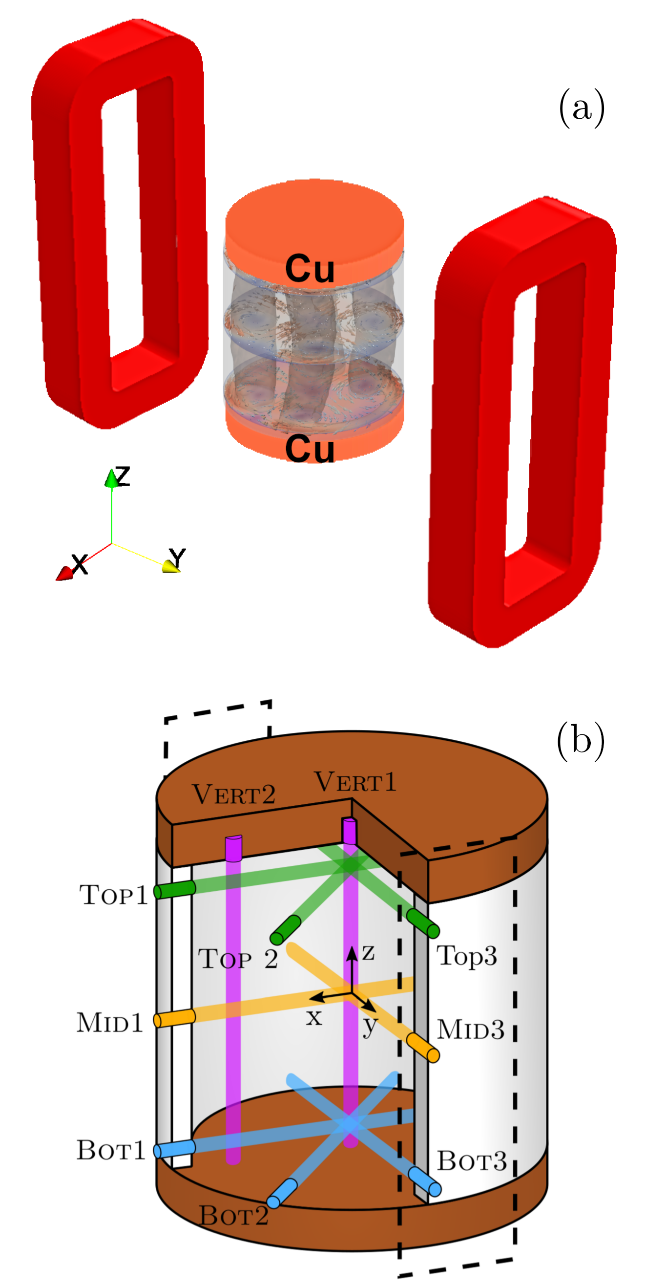
Figure 1: Schematic setup of the experiment. (a) Two coils (red), fed by an AC current with $25$ Hz, produce a tide-like $m=2$ forcing in the cylindrical container filled with GaInSn. In the case without RB flow, the tide-like force generates 4 rolls which are also shown POF2020 . (b) Configuration of the UDV sensors and the measurement paths. Here, the arrangement of the excitation coils lying on the y-axis is only indicated by the dashed lines.

The sidewalls, made of polyether ether ketone (PEEK), are considered thermally and electrically insulating. On top and bottom, the cylinder is bounded by two uncoated copper plates with 220 mm diameter and a thickness of 25 mm. During the RB experiments the bottom plate is electrically heated while the top plate is watercooled. If not otherwise stated we work with a temperature difference of 5 K which is ensured by a thermostat. This temperature difference corresponds to a Rayleigh number $Ra=\alpha gH^{3}\Delta T/\nu\kappa=1.03\times 10^{-7}$ with thermal expansion coefficient $\alpha$ and gravitational acceleration $g$. The turnover time $t_{to}=L/\overline{u}_{LSC}$ with $L$ being the LSC path length for this state is estimate to be around 50 s. From the electromagnetic point of view both copper plates are considered to be in perfect electrical contact with the GaInSn. Due to the large ratio (appr. factor 18) between the thermal conductivities of copper and GaInSn and a small size ratio resulting in a low Biot Number $\ll 1$Schindler2022 , the temperature distribution at the interface between the two materials is considered homogeneous.

Just as in POF2020 , the tide-like $m=2$ forcing is generated by AC-currents through two rectangular, stretched coils which are situated on opposite sides of the cylinder as delineated in Fig. 1a. Each has 80 turns, 10 pancake layers, a total inner height of 350 mm and a mean distance between the long leg and the x-z centre plane of 145 mmPal2009 ). The distance between the central pancake layer and the cylinder centre is 285 mm. When a current is applied to the coils a magnetic field is generated which is symmetrical to the centre plane. A tunable AC power supply is used to create an alternating current with defined amplitude and frequency in the coils. Throughout this paper, this frequency will be fixed to 25 Hz which was optimised previously POF2020 . The polarity of the coils is assigned in a way that the magnetic field is concordant in both solenoids. This configuration has turned out advantageous for generating the desired flow structure StepanovStefani2019 .

Although the cylinder is also equipped with thermo-couples, in this paper we exclusively rely on the velocity signals measured by 8 MHz Ultrasound Doppler Velocimetry (UDV) sensors, whose configuration around the vessel is illustrated in Fig. 1b. The sampling period for all the sensors is about 2.45 s for the experimental data and 1 s (plain RB) and 2 s for the numerical data. Referring to the bottom interface between copper and GaInSn, the measurement planes “Bot”, “Mid” and “Top” are located at heights of 10, 90 and 170 mm, respectively. At each height, two sensors called “1” and “3” are placed with an angle of $\pi/2$ between them (the additional sensors “2” are not utilized in the following). Two further UDV sensors for measuring the vertical flow component are placed in the top copper plate at radial positions $r/R=0$ and $r/R=0.8$. Of those, we will only utilize data of “Vert2”, situated close to the lateral boundary. A more detailed description of the cell can be found in Zuerner2019 .

II.2 Numerical scheme

The flow in the cell is computed, using OpenFOAM 6 openfoam , by solving the incompressible Navier-Stokes equation and the continuity equation

$$\rho\frac{\partial\bm{u}}{\partial t}+\rho(\bm{u}\cdot\nabla)\bm{u}=-\nabla p+\rho\nu\nabla^{2}\bm{u}+\bm{f}\,,$$ (1)

$$\nabla\cdot\bm{u}=0\,,$$ (2)

wherein the force $\bm{f}$ is a sum of the electromagnetic force generated by the AC current in the coils and the buoyancy force due to the imposed temperature difference between the lower and upper copper plates:

$$\bm{f}=M(t)\bm{f}_{EM}+\bm{f}_{buoyancy}\,.$$ (3)

The thermal convection is modelled by the Boussinesq approximation which provides the buoyant force $\bm{f}_{buoyancy}$ to the Navier-Stokes equation. Since the resulting flow speeds are low (a few mm/s), the corresponding small magnetic Reynolds numbers ($Rm\sim 10^{-3}...10^{-2}$ ) allow us to decouple the magnetic field generation from the flow calculation.

We therefore pre-computed the Lorentz force

$$\bm{f}_{EM}=\bm{j}\times\bm{B}$$ (4)

by solving Maxwell’s equations in Opera 1.7opera2018 and added it as a vector field to the Navier-Stokes equation. To emulate a time-dependent tide-like forcing, this time-constant part $\bm{f}_{EM}$ of the Lorentz force is amplitude-modulated by the factor

$$M(t)=\sin^{2}(\pi f_{mod}t)$$ (5)

wherein the frequency $f_{mod}$ is chosen close to the natural frequency $f_{slosh}$ of the sloshing motion of the LSC (which is displayed below). To achieve a positive-defined sinusoidal modulation, i.e. $0<M(t)<1$, the sine function is squared and the natural frequency is halved. Figure 7 in POF2020 shows the spatial distribution of $\bm{f}_{EM}$ at the maximum $M(t)=1$.

The mesh utilized for the simulations consists of hexahedral cells with contracted cells at the walls where the no-slip condition ${\bf u}=0$ is implemented. For all numerical simulations of the combination of RB convection and tidal forcing, we used the results from a pure RB flow after 3000 seconds as starting point.

III Results

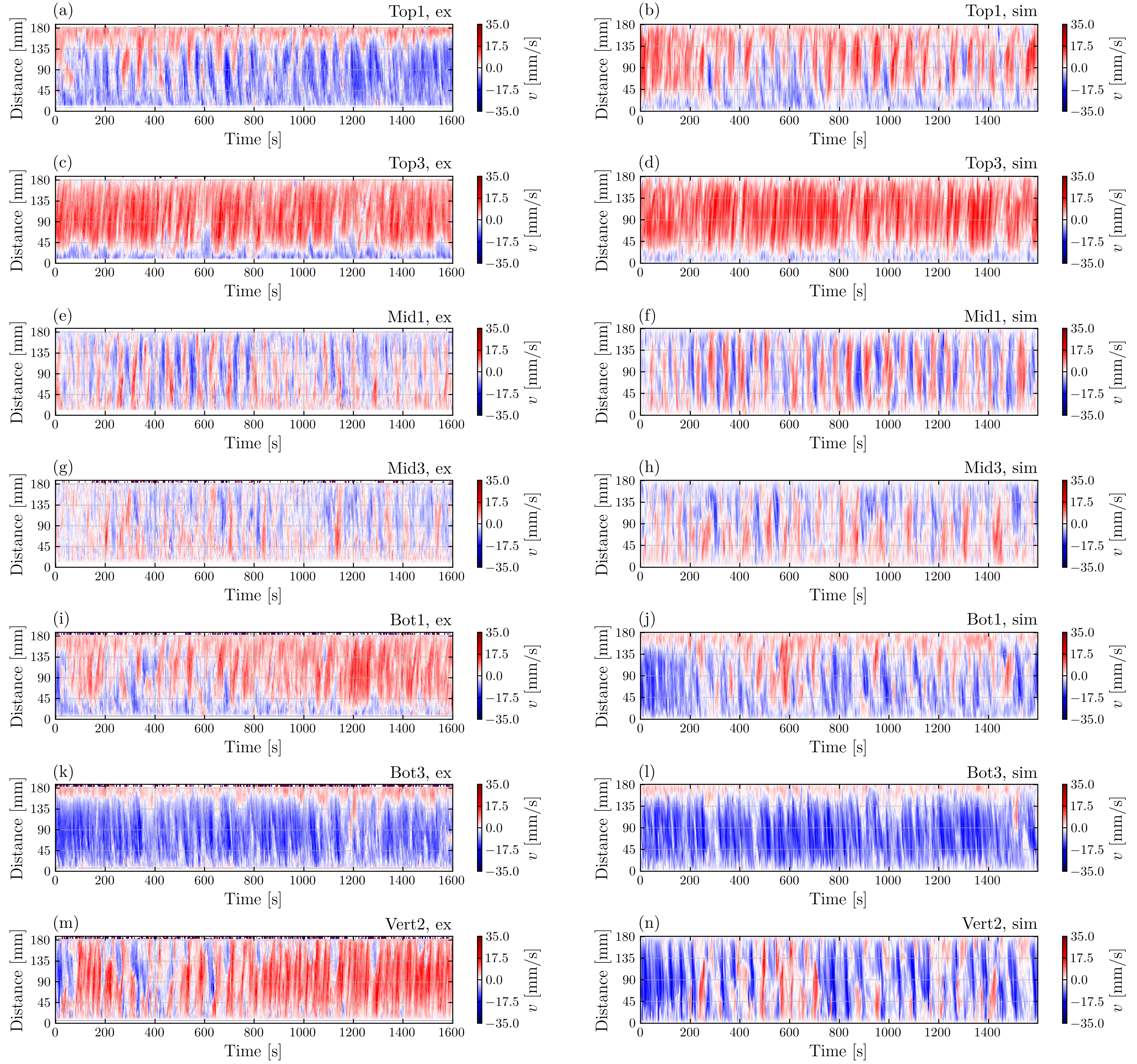
Figure 2: Contour plots of the velocities along the sensor beamlines for a coil current of 0 A (pure RB convection). The left column shows measurement data for seven selected UDV sensors, while the right column shows the corresponding virtual sensor data extracted from the simulation.

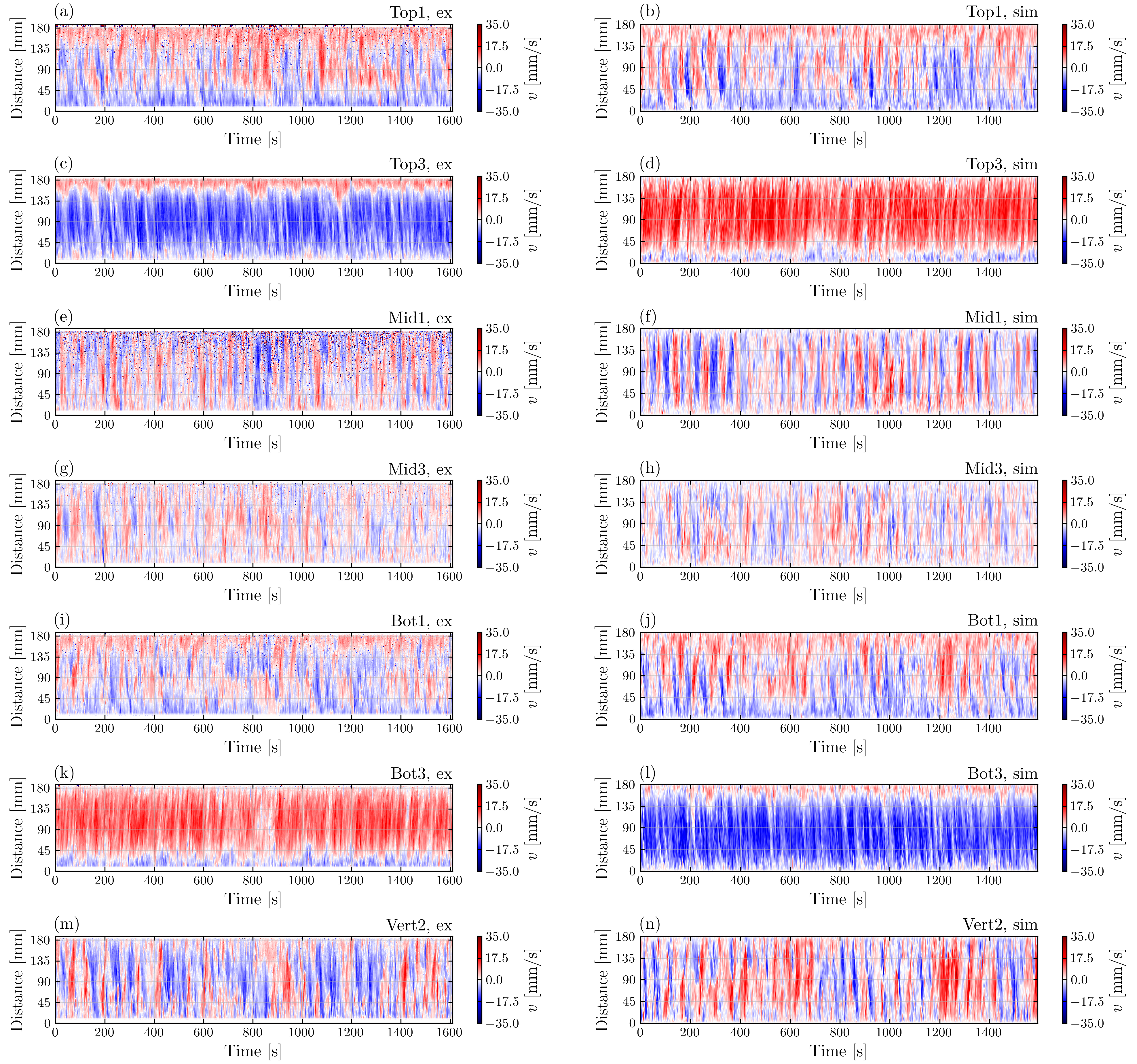
Figure 3: Same as Fig. 2, but for a coil current of 12.5 A.

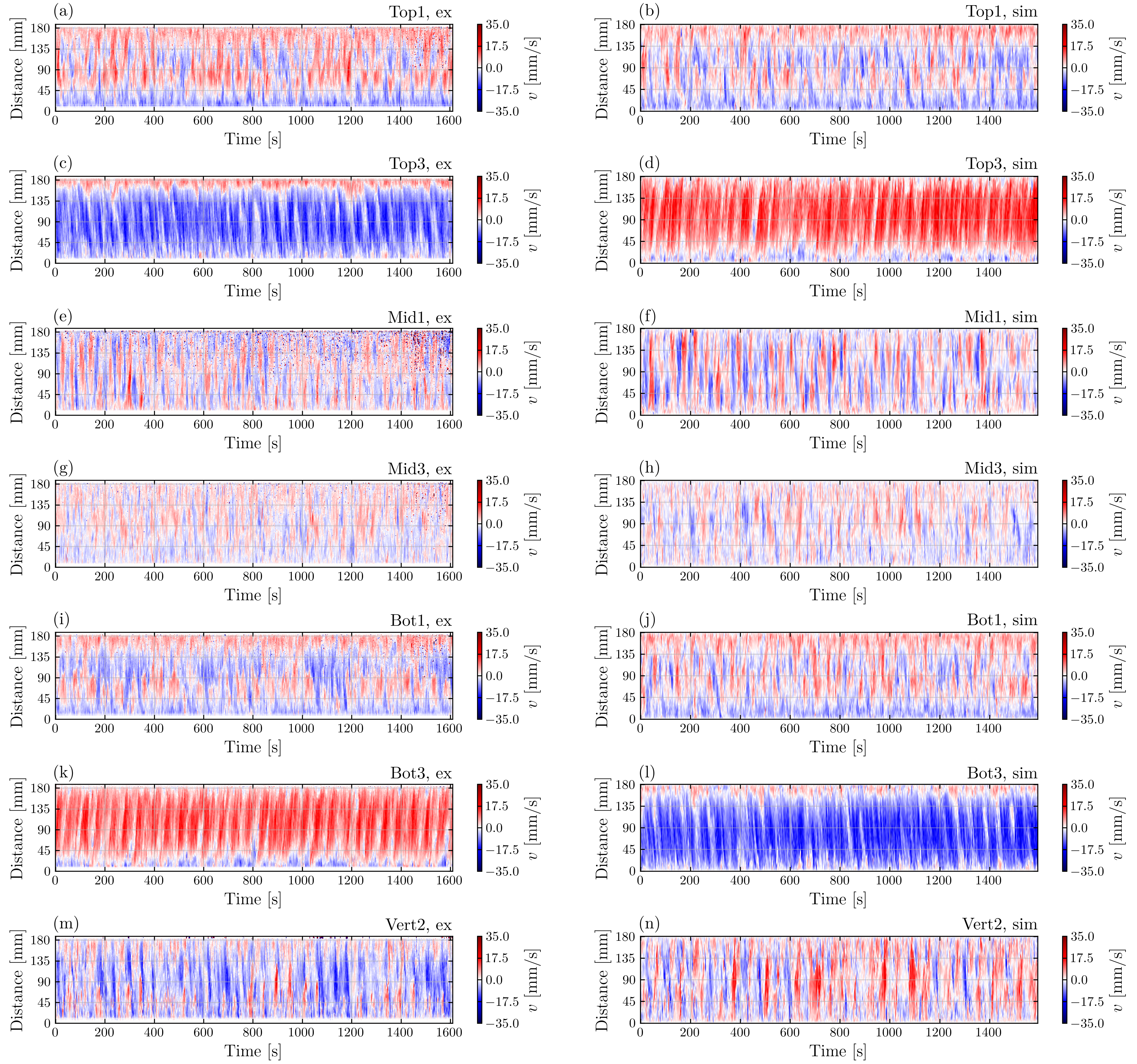
Figure 4: Same as Fig. 2, but for a coil current of 21.2 A.

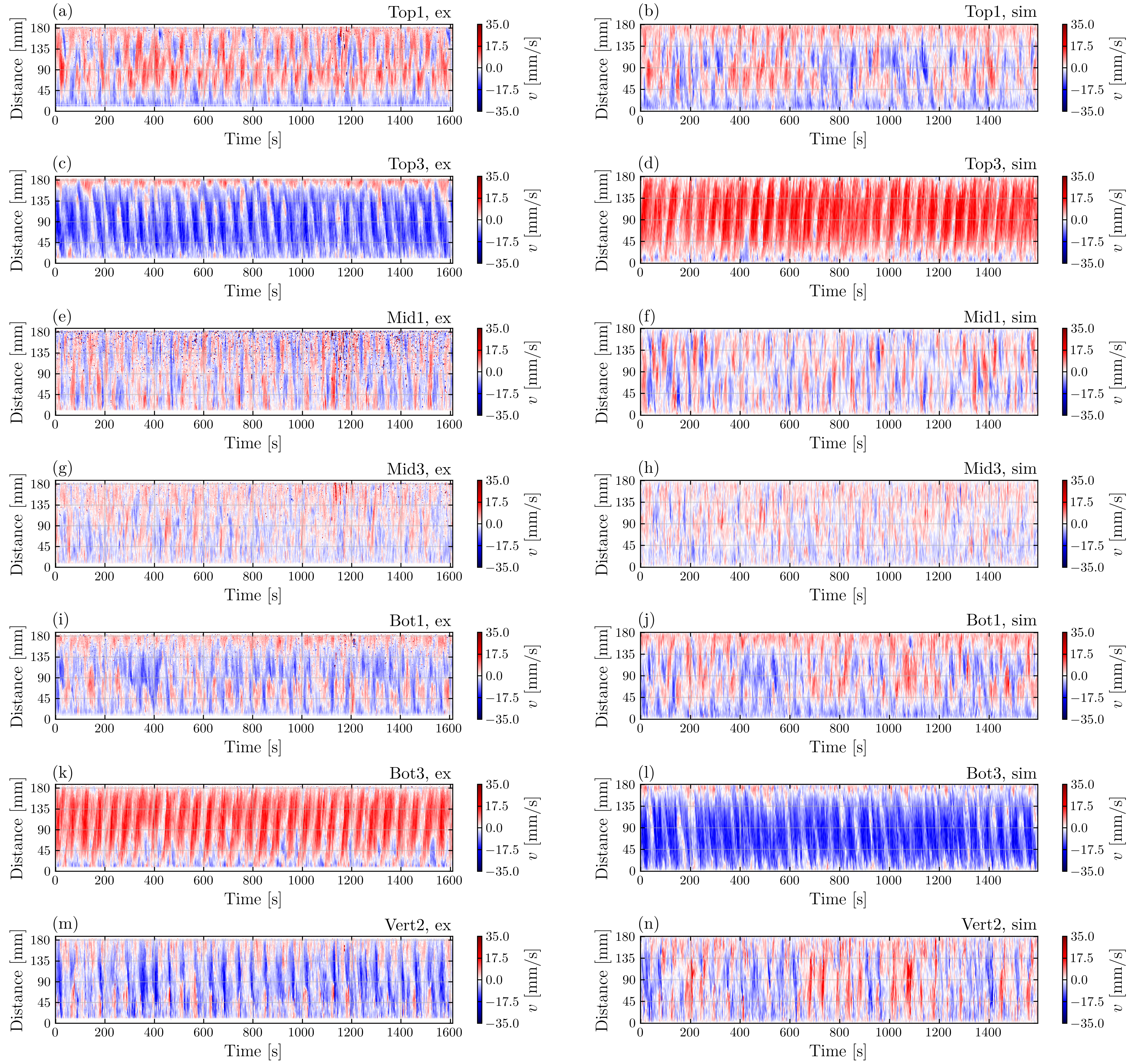
Figure 5: Same as Fig. 2, but for a coil current of 27.6 A.

Although a wide variety of frequency, current and temperature parameters has been explored in the experiments, in the following we focus on a RB flow with a temperature difference $\Delta T=5\,\mathrm{K}$ which corresponds to a Rayleigh number of $Ra=1.03\times 10^{7}$.

In all cases with forcing, the fundamental frequency of the coil current is fixed to 25 Hz, while the amplitude is slowly modulated with frequency $f_{mod}$. A setting of $f_{mod}=18\,\mathrm{mHz}$ has been chosen to be in the range of the natural sloshing frequencies of the LSC as mentioned before. The intention was, staying close to a possible 1:1 resonance, while being slightly off so a possible entrainment would be visible.
First, we present the UDV sensor data for four representative cases with increasing coil currents. This yields already a qualitative picture for the process under investigation. A following spectral analysis and forcing-signal-correlations elucidate possible causal relationships. Further insight is provided by evaluations of the simulated flow field, allowing for an attempt at a theory for the underlying mechanisms.

III.1 UDV data for four different coil currents

Here we present the velocity profiles measured along seven selected UDV sensor beams and compare them with the corresponding profiles of virtual sensors as extracted from numerical simulations. Specifically, we discuss the results for the four maximal coil current amplitudes of 0 A, 12.5 A, 21.2 A, and 27.6 A. The presented data are representative examples from, in some cases, much longer time series.

We start with the pure RB flow, i.e. with zero coil current. For seven selected sensors, Fig. 2 shows the contour plots (over time and UDV beam depth) of the actually measured signal (left column) and of the corresponding “virtual sensors” (right column). For the selected time frame of 1600 s, all sensors show velocities with amplitudes of some 30 mm/s, and short term oscillations with periods of appr. 50 s. The dominance of the flywheel-type LSC is clearly mirrored by the reciprocal flow direction (red versus blue) between sensors “Top1” and “Bot1”, as well as between “Top3” and “Bot3”. Whenever the flow is directed towards (blue) the sensor at the top, the corresponding signal at the bottom sensor is red, indicating a motion away from the sensor. Appropriately, the “Vert2” sensor observes, for most of the time, a downward motion (red). The signals from the “Mid” sensors are noticeable weaker. What they actually measure is not the flywheel itself, but basically its lateral deflection, which corresponds to the sloshing motion of the LSC with its periodicity of appr. $50$ s. On longer time scales not shown here, we also observe an azimuthal drift of the main LSC direction, as well as sudden cessations with direction change. Qualitatively, the virtual sensors on the right hand side show a very similar behaviour, including the $\sim 50$ s periodicity. Yet, in view of the random direction of the LSC and its long-term drift, a perfect agreement of all details cannot be expected.

The next plot, Fig. 3, shows the corresponding (real and virtual) sensor data for a coil current of 12.5 A. While neither the velocity amplitude nor the $\sim 50$ s periodicity have much changed from the 0 A case, we observe now a clear regularization of the flow, with the LSC constantly oriented in $y$ direction, i.e., along the sensor path of “Top3” and “Bot3”. This effect has already been noted in Roehrborn2022a ; Roehrborn2022b and is confirmed in this dataset. The fact that the direction of the LSC in the numerical simulation happens to be contrary to that in the experiment (red versus blue in “Top3”) merely results from random initial symmetry breaking and is of no consequence for the analysis. Sloshing in $x$-direction is now most strongly expressed in the “Mid1” data, while the numerical data shows slightly more regularity than the experimental one. As for the “Vert2” sensor, one can observe exchanging upward and downward streams resulting from the rotation/torsion of the LSC. Noteworthy is also the change in flow structure in the “Top1” and “Bot1” data. It switches from a mainly unidirectional flow (as in Fig. 2) to a four-section structure, which will become even more pronounced with increasing coil currents.

At 21.2 A (Fig. 4) the regular patterns become obvious, particularly visible in the “Top3” and “Bot3” data. Despite being accordant to the forcing, as will be shown below, they are unlikely to be just a measurement of the forcing, as the particular sensors “look” perpendicular to the main forcing direction. In particular, the unimodal flow direction is not what would be expected from a purely forced flow, as in POF2020 . Interestingly, also a somewhat higher frequency in “Mid1” emerges which will be discussed in more detail further below.

Finally, the 27 A case (Fig. 5) exhibits a very stable periodicity, pointing to a sort of asymptotic synchronization behaviour. The four-section structure in “Top3” and “Bot3” is now very pronounced.

III.2 Fourier spectra

Having observed an increasing flow regularity in the previous section, we asks now what frequencies are included and how they relate to the forcing. For that purpose, we discuss the Fourier spectra of several locations in the cylinder. Specifically, for “Top3”, “Bot3”, “Mid1” and “Vert2” we will focus on the central segments around 90 mm, averaged over the depth between 85 mm and 95 mm. For the “Mid1” sensor, we will additionally observe points centered around 40 mm, and 140 mm, likewise averaged over the surrounding 10 mm. Along the time axis, segments of ca. 1600 s are selected identical to the ones displayed in section III.1. The resultant time series are detrended and a von Hann window of the same length as the series is applied before the data are passed to NumPy’s real-valued discrete Fourier Transform function “rfft”. The shown periodograms are to be interpreted as examples only. As the turbulent flow (of $Re=\bm{u}D/\nu\approx 10^{5}$) has an inherently chaotic element to it, the results can vary depending on the observed time frame (particularly for the low current values).

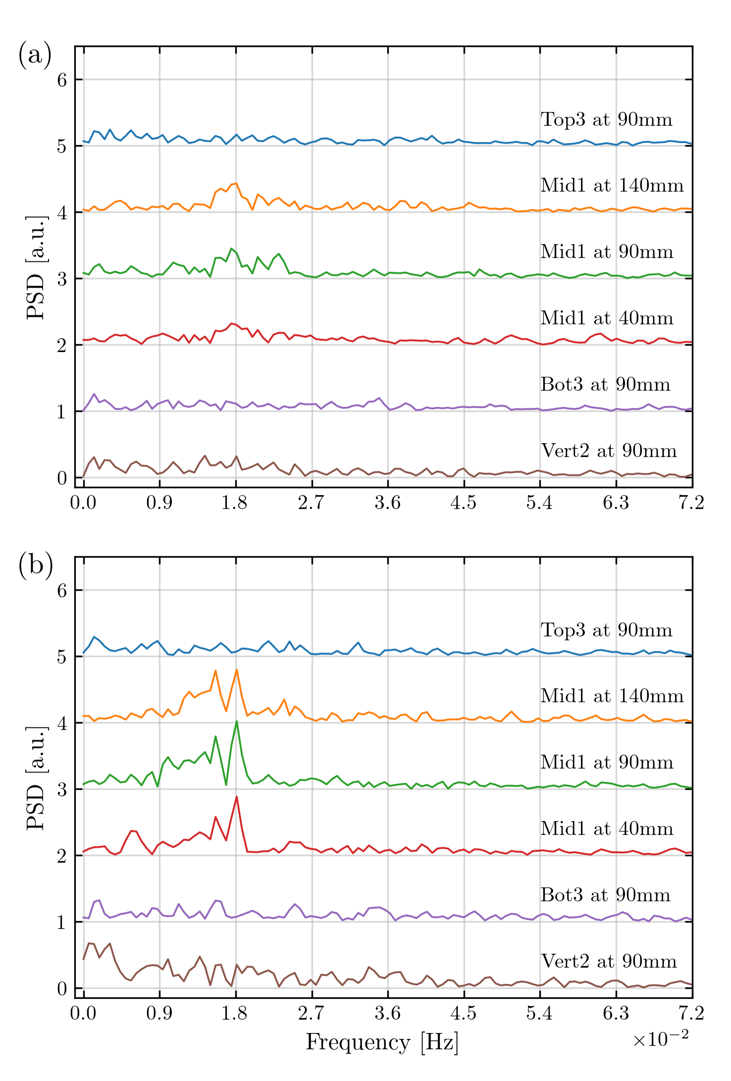
Figure 6: Power spectral density (partly shifted) of six data sets from four sensors, extracted at various depths from Fig. 2, for a coil current of 0 A. The upper panel corresponds to data from the real sensors, the lower panel to those of "virtual sensors" from simulation.

Let us begin, in Fig. 6, with an analysis of the pure RB case ($0$ A). In view of long-term wanderings of the LSC in this case, the corresponding data in Fig. 2 has been chosen from a longer time series such that the LSC is pointing roughly in the direction of the “Top3” and “Bot3”sensors. The FFTs of the center flow show a rather broad maximum around 18 mHz (corresponding to 55.56 s) which is the typical frequency of the sloshing/torsional motion in our case. This is why it has been chosen as the forcing modulation period in this study. Such a peak actually can also be found in the angle data, a measure used in previous investigations LSC-Till-2019 .

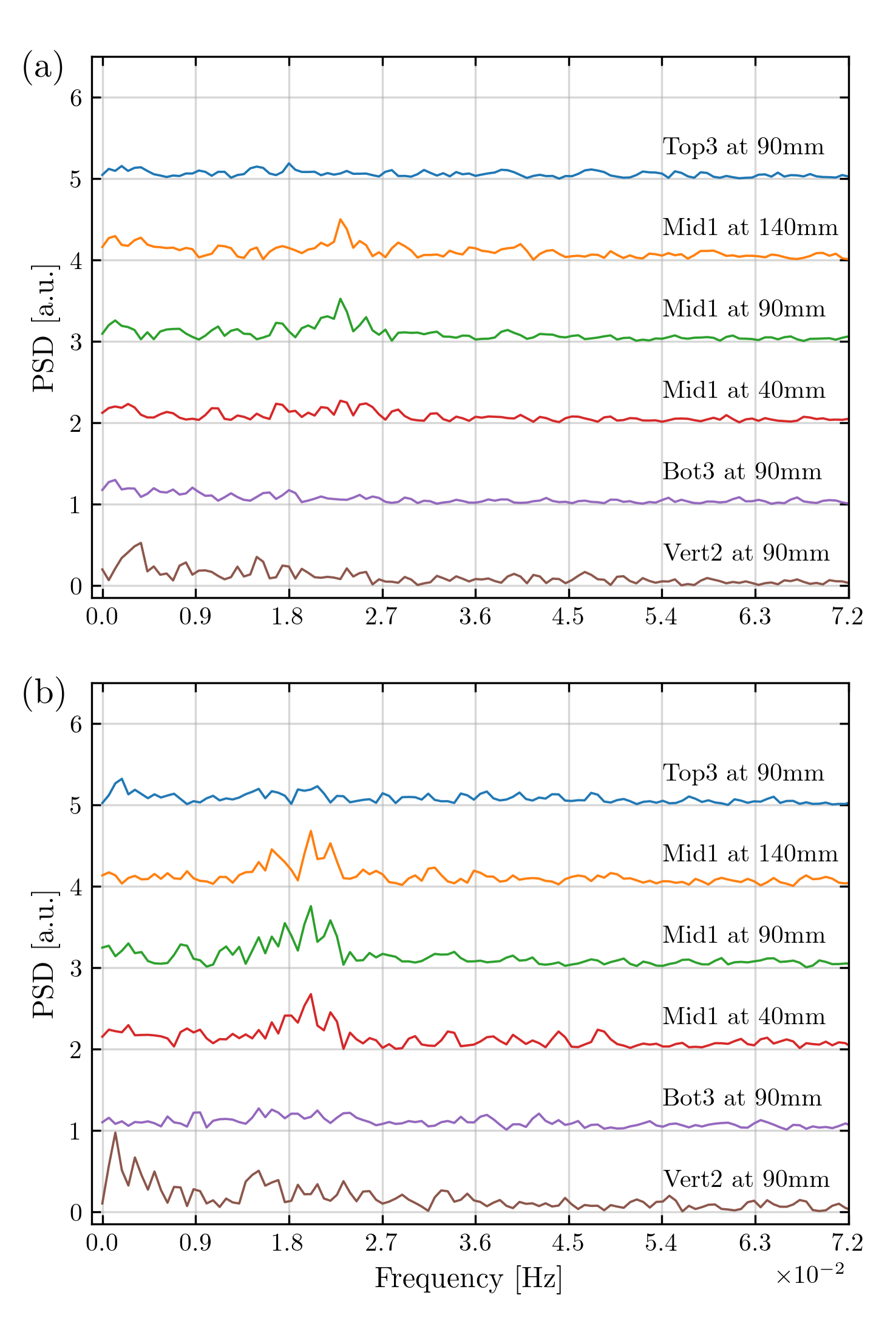
Figure 7: Same as Fig. 6, but for 12.5 A.

At 12.5 A the peaks of the “Mid1” sensor start to shift towards higher frequencies, as can be seen in Fig. 7. The other measurement points still seem to be much too irregular in behaviour for the FFT to pick up anything worth mentioning.

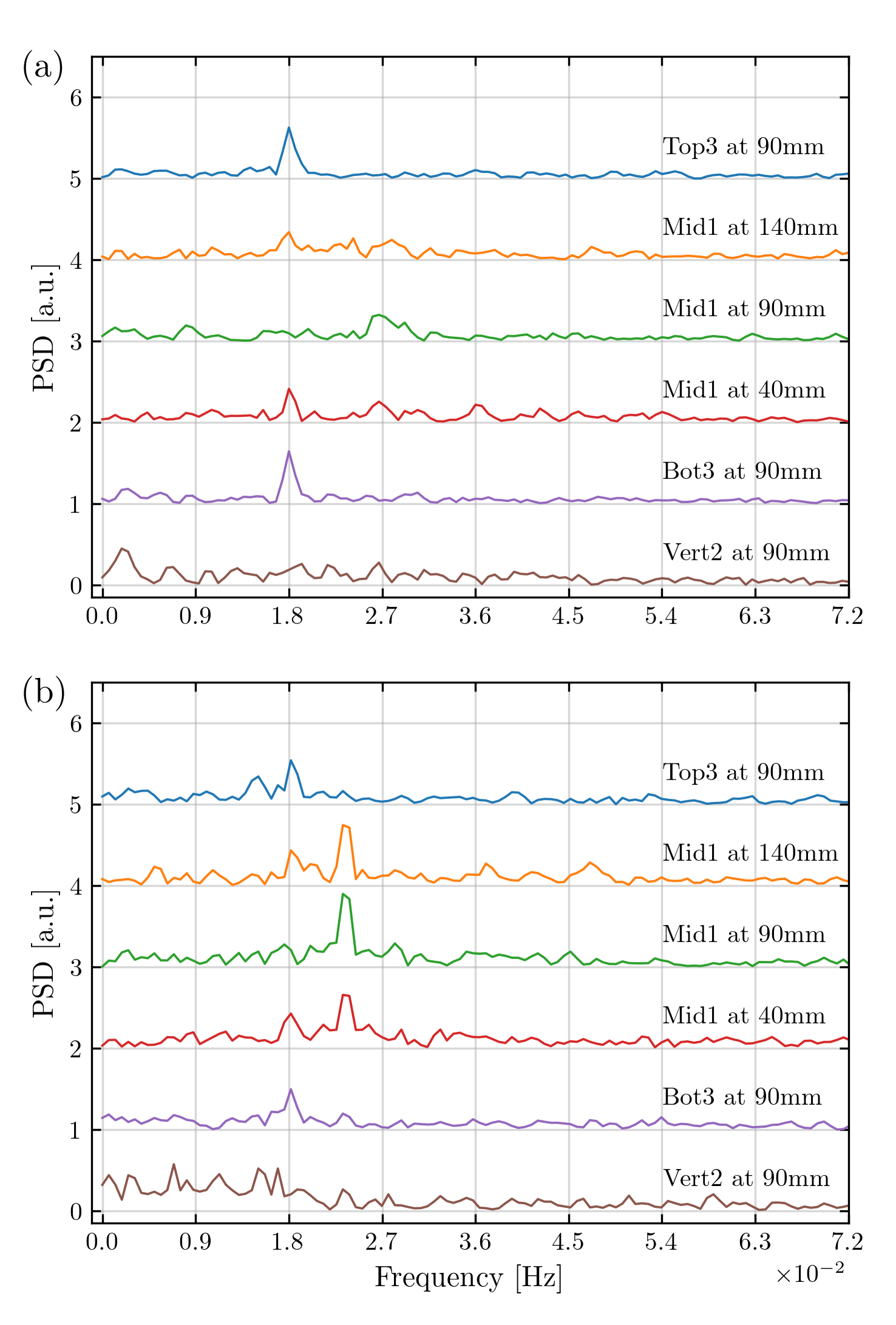
Figure 8: Same as Fig. 6, but for 21.2 A.

Increasing the coil current further to 21.2 A, Fig. 8 displays now prominent peaks at the forcing frequency of 18 mHz, both for experiment and simulation. The points roughly one fifth from the wall in “Mid1” also see this frequency in addition to the faster periods. Those faster periods also shift a little further up the scale, which seems to be consistent behaviour.

Further increasing the coil current to 27.6 A shows the same pattern with an even more expressed forcing period in the “Top3” and “Bot3” data (Fig. 9). At this stage it is even expressed in the “Vert2” experimental data.

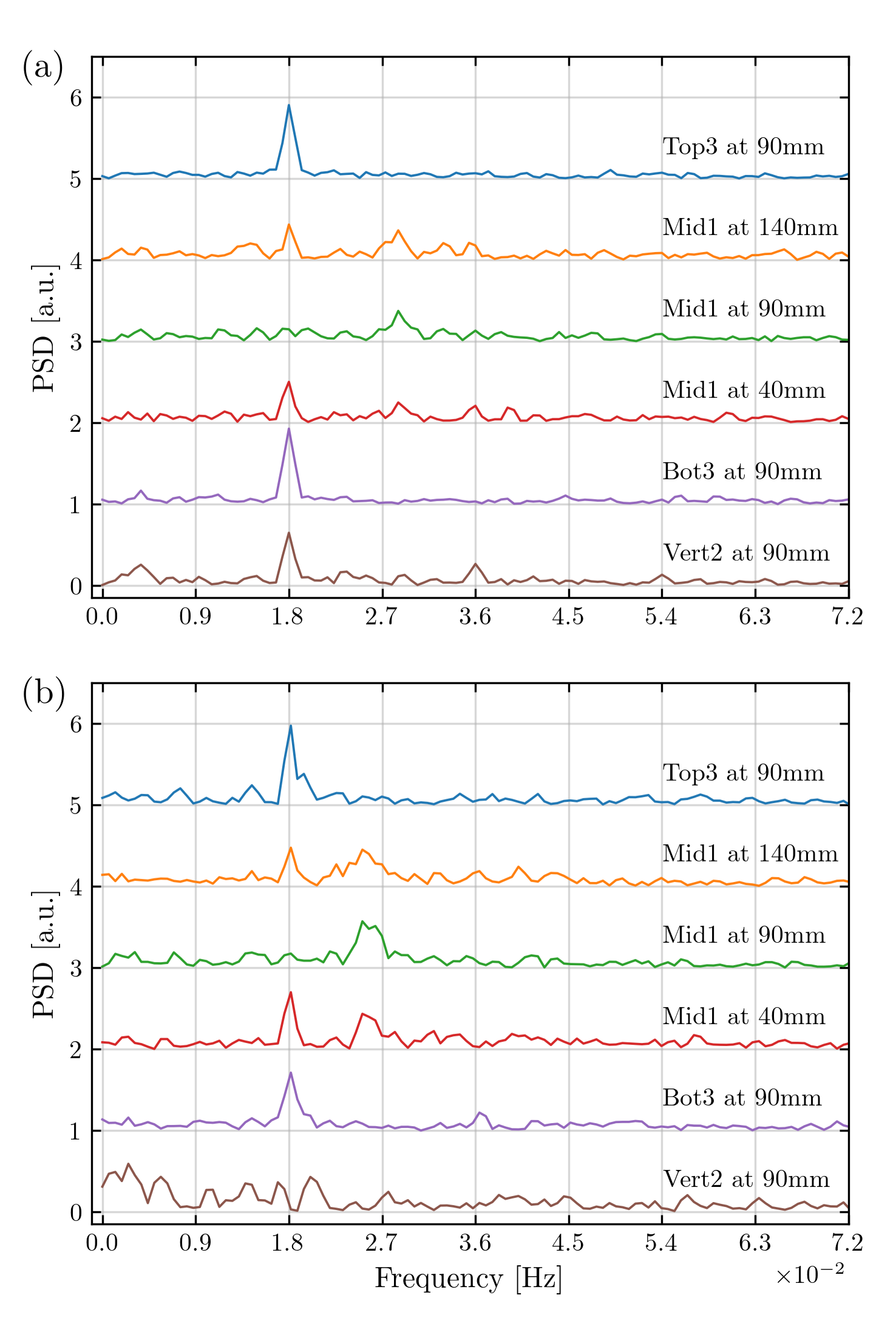
Figure 9: Same as Fig. 6, but for 27.6 A.

We conclude that the increasing Lorentz-forces clearly leave their mark in the FFT spectra as well. A remaining question is, how the fluctuation at the cylinder centre evolves. As a first glance, Fig. 10 depicts the strongest frequencies for the 90 mm data divided by the modulation frequency of 18 mHz. It is not a perfect measure and subject to statistical fluctuations, but suggests a continuous increase. And while the 37 A data points are not quite reliable due to small peaks, further simulations suggest a saturation beyond that current. At any rate, the observed periods are somewhat unstable and thus the frequency peaks are not sharply expressed.

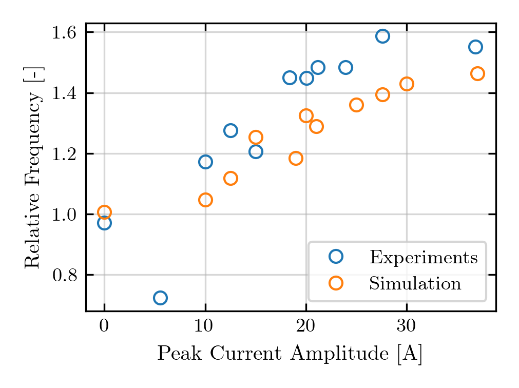
Figure 10: Analysis of the strongest frequencies in the Mid1 sensor at 90 mm for experiments and numerics, relative to the forcing modulation frequency of 18 mHz. The data points at 37 A are questionable, as the peaks are not at all pronounced.

III.3 Transition to synchronization

With a first characterization at different forcings at hand, we now discuss the synchronization in a more quantitative manner. For that purpose, we assess the correlation between the force signal $M(t)$ according to Eq. 5 and the velocity around the centre of “Bot3”. The latter data is chosen because the measured LSC velocities are perpendicular to the forcing and the sensor is delivering a low noise signal throughout all measurement runs. It also shows the strongest forcing response in the contours 2-5. The employed metric is Pearson’s empirical correlation coefficient:

$$r_{k}(x,y):=\frac{\sum_{i=1}^{n}(x_{i}-\overline{x})(y_{ik}-\overline{y}_{k})}{\sqrt{\sum_{i=1}^{n}(x_{i}-\overline{x})^{2}\sum_{i=1}^{n}(y_{ik}-\overline{y}_{k})^{2}}}$$ (6)

where $x$ is a 27 periods long segment of the forcing envelope curve, y is the formerly mentioned velocity data, from which a 29-period length is selected, and k denotes the lag between the correlation signals. During correlation, the signal y is shifted across signal x and only the part of x is used that has a corresponding value in the y data. In order for this to be executable, both signals exhibit an identical temporal sampling.

As the forcing signal is 27 periods ($\equiv$1500 s) long, only a long-term coherent effect will yield a high correlation coefficient and thus hint at synchronization. If the synchronicity is weak and the periodic velocity’s phase drifts with respect to the forcing or looses its periodic structure, the correlation coefficients will be small.

As two periods of lagging were chosen, when plotted over the lag distance the resultant coefficients resemble more ore less two periods of a sinusoid for all datasets (including plain RB). Thus, the maximum correlation and average phase difference can be estimated. Non-linear fitting of a sinusoid has been used to estimate the phase lag.

In Fig. 11 those maximal coefficients and corresponding phase lags are plotted against the coil current. The blue triangles are taken from measurements, while the grey crosses are values from the numerical data. The orange circles represent the average of the grey crosses for one current value.

Evidently, at low currents there is almost no correlation between the forcing and the flow (for the plain RB case, a proxy sine function with 18 mHz was used). Then, the correlation rises steeply between 10 A and 25 A, after which it reaches a sort of plateau. As long-term coherence is required for such high values to occur, we take this as strong evidence for a synchronization effect at play.

Nevertheless, the phase difference is quite large with more than half a period lying between the maximum of the forcing and the maximum of the flow velocity. This might hint at the synchronization mechanism working in a part of the cylinder which is away from the centre.

While the phase in Fig. 11(b) appears to be very steady even starting at 10 A, there is, obviously no reasonable phase relation to be defined for lower currents. Since the “coherence length” is rather short, the maximal correlation coefficient is strongly dependent on the chosen time frame. A first attempt on characterizing the underlying statistics has been made using a sort of bootstrapping on the numerical data. There, longer datasets were available and more than one interval of 1500 s could be evaluated. The result are the grey crosses in Fig. 11.

For high currents, the crosses have a consistently small spread, which gives some validity to the former interpretation of the data. Yet, the correlation does not reach exactly one, which is due to noise from turbulence always contained in the data.

Even though a synchronization effect is readily apparent, the actual process facilitating it has to be further illuminated.

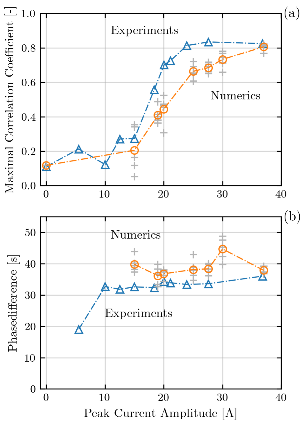
Figure 11: Onset of synchronization with increasing current. (a) Maximum of the empirical correlation coefficient of sensor “Bot3” with the function $M(t)$ according to Eq. (5). (b) Phase shift between the two signals where the maximum of the correlation occurs. In both panels, the blue triangles represent experimental results, while the grey crosses represent the numerical results for multiple intervals on the same dataset. The orange circles depict the average over the crosses for each current amplitude.

III.4 Flow geometry and helicity synchronization

In this section we will have a closer look on the actual mechanism of the synchronisation. For that purpose, we mainly rely on the numerical simulations which allow to analyze the flow in much more detail than it would be possible from the limited number of sensors used in the experiment. This applies, in particular, to the helicity of the flow which can only be quantified by numerical data. However, the good correspondence between numerics and experiments presented so far makes us confident about the physical relevance of the numerical simulations.

As previously stated, the flow geometry changes from a plain RB case to a forced case. In Figs. 12 and 13, the flow is illustrated in 9 panels distributed over one period of 55 s. For the pure RB case, in Fig. 12 the panels show the typical sloshing and torsional motion associated with the movement of the LSC in the volume. The forced case with $30$ A, shown in Fig. 13, reveals a more complex behaviour. On the mid-height plane, a back and forth motion is visible but has additional components superimposed. On the top and bottom planes, the flow seems to be parted in two, along positive and negative $x$, whenever the forcing starts to act. On closer inspection it appears that the LSC is strong on one side and then switches sides without visibly crossing the center over the course of one period. The large scale structure of the LSC seems to become more complex with those branching flows.

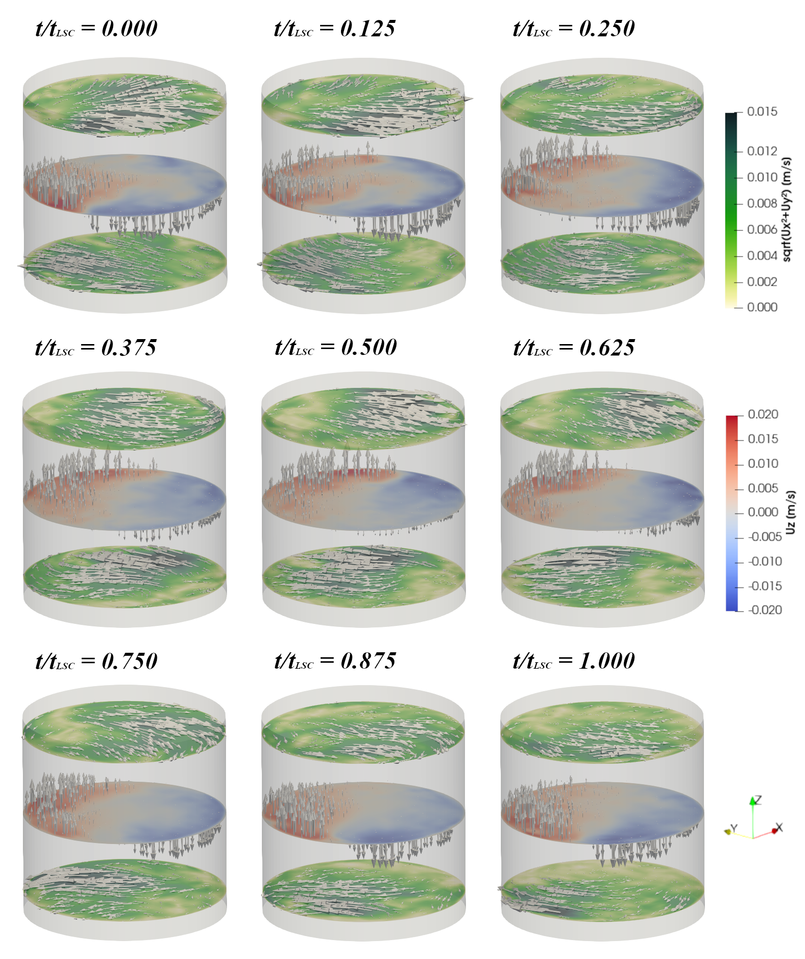
Figure 12: Illustration of the vector flow field for a coil current of 0 A (pure RB convection). The 9 panels cover a typical sloshing period of 55 seconds, during which the LSC undergoes a “round trip”. The upper and lower planes show the horizontal component of the velocity (gray arrows), including its intensity (color). The plane at mid-height shows the corresponding vertical velocity component.

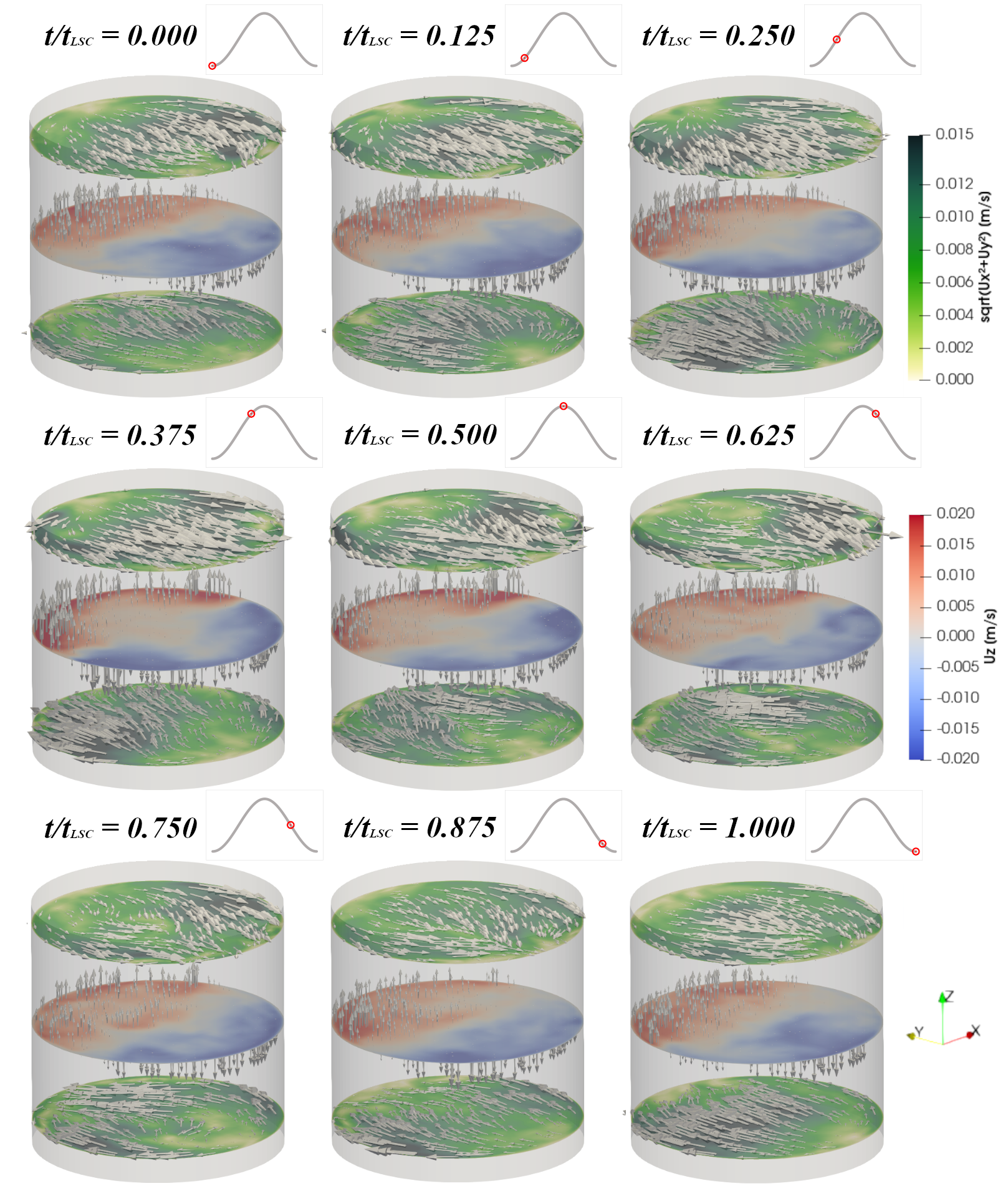
Figure 13: Same as Fig. 12, but for a coil current of 30 A.

There are several ways to interpret this behaviour. Looking at how the alternation of sides in plume formation is regularized, an interaction of the Lorentz-forces with the internals of the RB process is suggested. Further investigation is required to exclude this possibility.

Nevertheless, turning to the helicity we can find another mechanism. In order to understand this concept, we have to make a few distinctions beforehand which are illustrated in Fig. 14. In addition to the full helicityMoffatt2018

$$H=\int_{V}\bm{u}\cdot\omega dV,\quad\mathrm{with}\ \omega=\nabla\times\bm{u}$$ (7)

integrated over the entire volume $V$, we consider also the partial helicities $H^{-}$, integrated over the restricted volume with $x<0$, and $H^{+}$, integrated over $x>0$. Furthermore, we distinguish between the two helicity density contributions $h_{x}=u_{x}\omega_{x}$ (red) and $h_{z}=u_{z}\omega_{z}$ (green), whose volume integrals are denoted by $H_{x}$ and $H_{z}$, respectively. Roughly speaking, the first one, $h_{x}$, represents the projection of the vorticity $\omega_{x}$ of the LSC on its sidewise motion $u_{x}$ (presupposing that the LSC is mainly directed in $y$-direction, which is safely guaranteed only in the synchronized regime). The second one, $h_{z}$, represents the projection of the vorticity $\omega_{z}$ of the four rolls (arising from the m=2 forcing POF2020 ) on the vertical component $u_{z}$ of the LSC which penetrates them. The third contribution, $h_{y}=u_{y}\omega_{y}$ has not such a clear interpretation and is, therefore, skipped in the following.

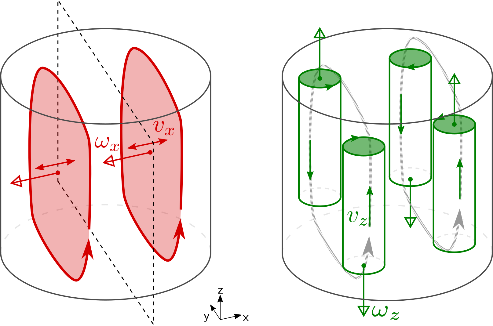
Figure 14: Illustration of the main contributions to the helicity, $h_{x}=u_{x}\omega_{x}$ (red) and $h_{z}=u_{z}\omega_{z}$ (green).

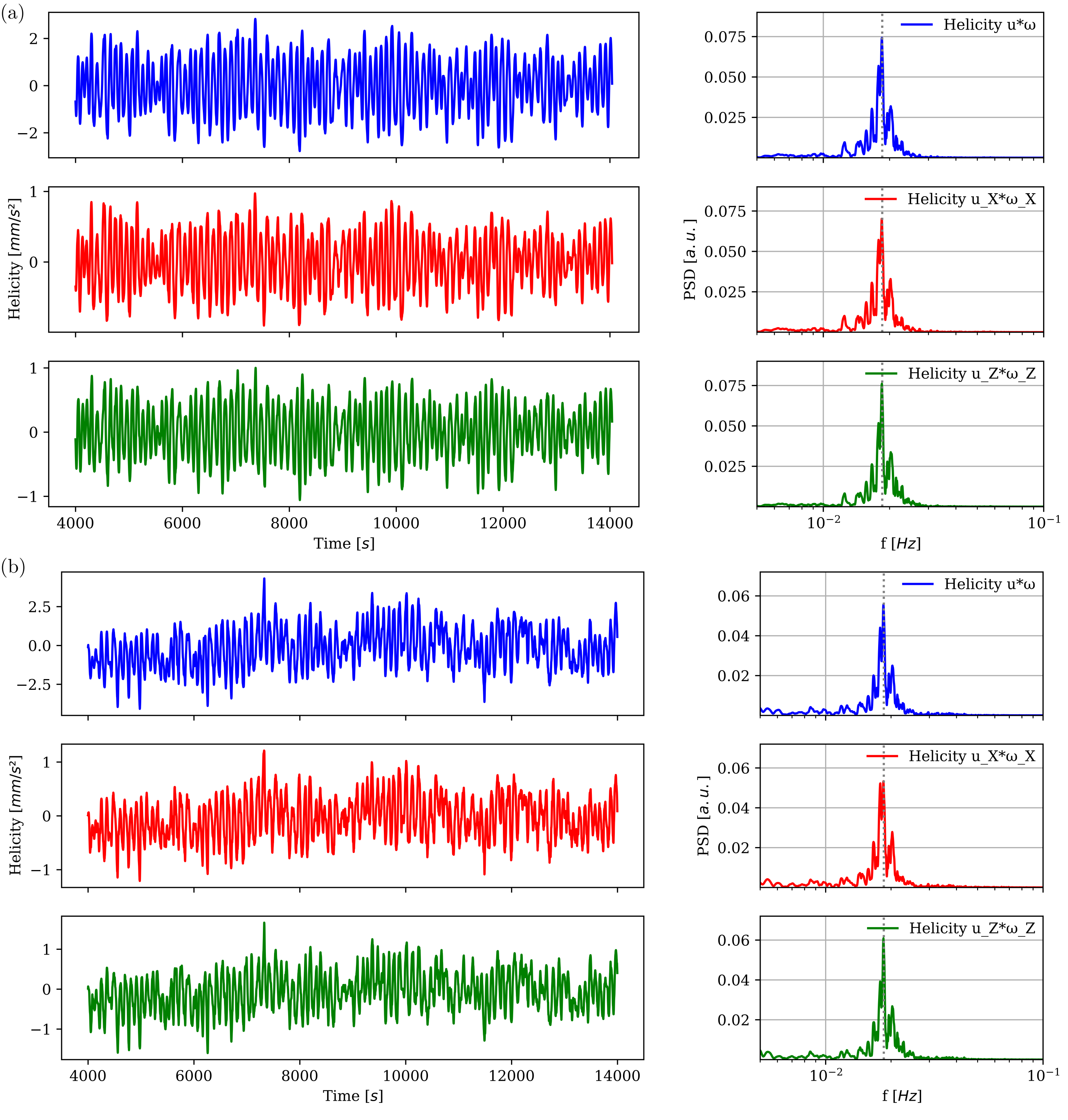
Figure 15: Time series (left) and FFTs (right) of the helicities $H$ (here normalized by the volume) in the plain RB flow. Pane (a) contains helicities calculated over the full volume, while in pane (b) only one half cylinder (negative x-values) is considered. The rows in each pane relate the full helicity $H$ (blue) and the partial contribution $H_{x}$ (red) and $H_{z}$ (green). The other half of the cylinder (positive x-values) yields comparable results and is therefore not shown.

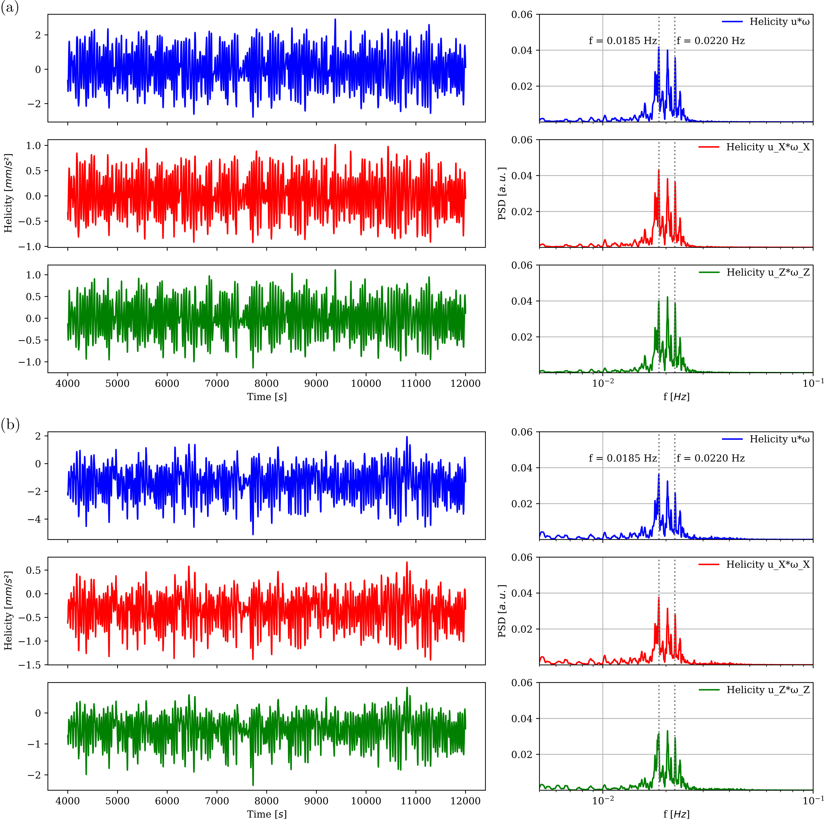
Figure 16: Same as Fig. 15, but for a coil current of 12.5 A.

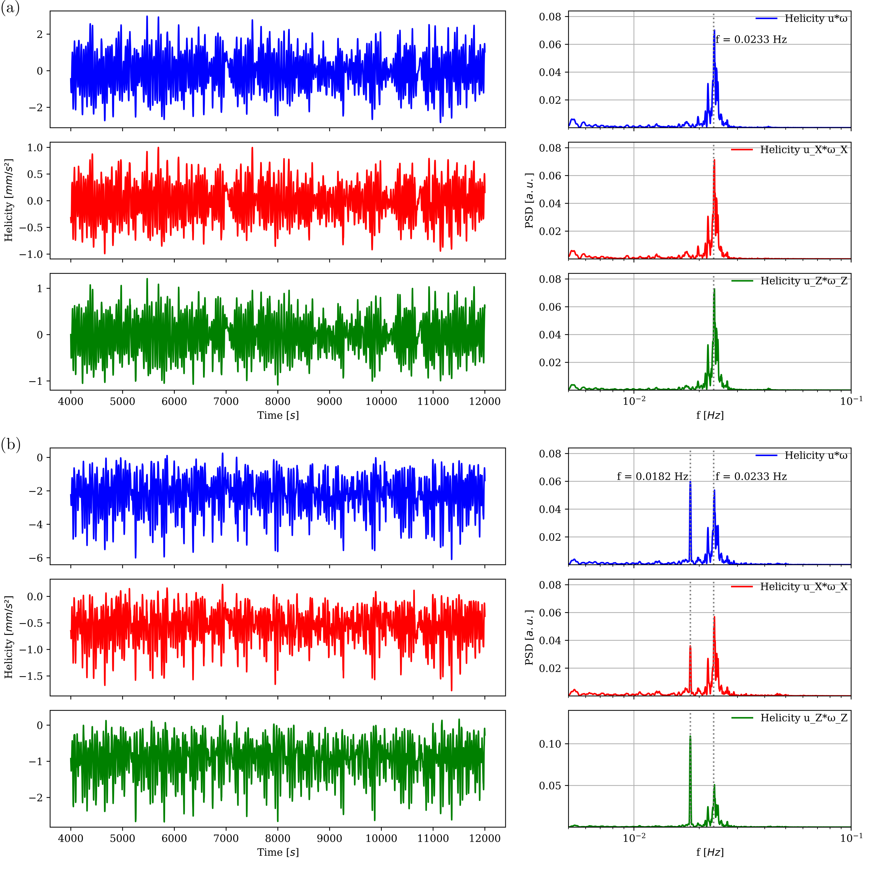
Figure 17: Same as Fig. 15, but for a coil current of 21.5 A.

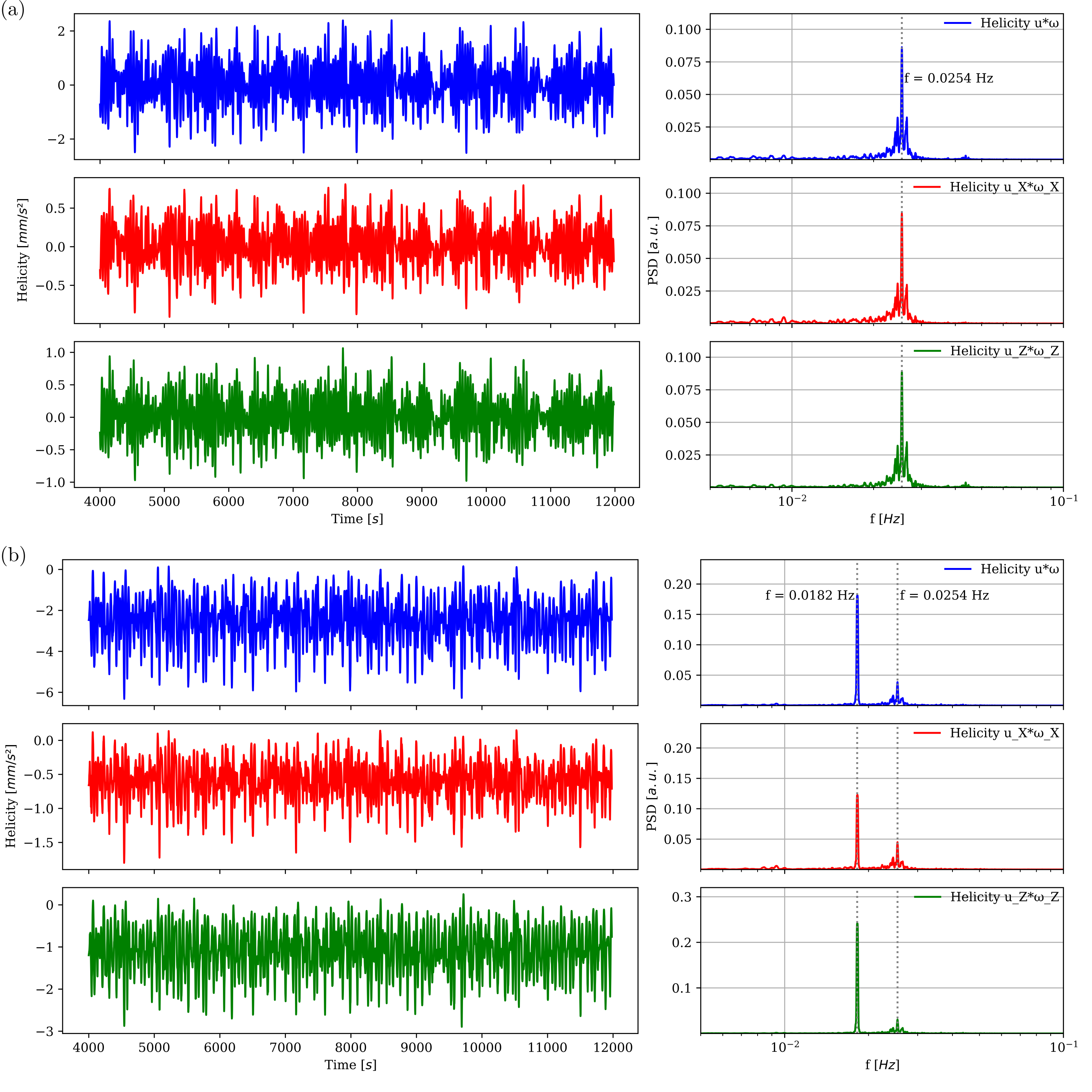
Figure 18: Same as Fig. 15, but for a coil current of 27.6 A.

We start again, in Fig. 15, with the pure RB case. Its left column exhibits time series of various helicity components, the right column shows the corresponding FFTs. The three rows of panel (a) show helicities averaged over the entire volume, while the rows of panel (b) show the corresponding partial helicity $H^{-}$ for the restricted volume with $x<0$ (we skip $H^{+}$ for $x>0$ as its graph looks similar to $H^{-}$, except with opposite sign). What we observe here in all FFTs is a rather broadband distribution, mirroring the sidewise motion of the LSC with its main, but not very sharp sloshing frequency.

For the next case of 12 A (Fig. 16), things are starting to change. All FFTs now show peaks at the synchronizing frequency of 18 mHz and also previously mentioned higher frequencies (see section III.2).

Going over to the case with 21.5 A as shown in Fig. 17, we observe even more drastic changes. All FFTs now exhibit extremely sharp peaks but with a decisive difference between the full-volume helicity $H$ and the half-volume helicity $H^{-}$. In the former, only a higher frequency at 23 mHz is apparent, while in the latter, a strong and narrow peak remains at the forcing frequency of 18 mHz.

At 27.6 A, which corresponds the to the “fully synchronized state”, the distinction becomes more or less complete. In difference to the full-volume version, the half-volume helicity $H^{-}$ of Fig. 18(b) are now dominated by the frequency of the forcing modulation, with only a minor component at the higher frequency.

From this evidence we conclude that helicity synchronization indeed occurs. The two half-volume helicities $H^{-}$ and $H^{+}$ are synchronized by the external $m=2$ forcing. $H_{x}$ and $H_{z}$ contribute comparable shares and take control of the cycle. It is not only the (unsurprising) oscillation of $\omega_{z}$ of the four rolls directly driven by the $m=2$ forcing which in combination with the reciprocal sign change of $u_{z}$ translates to a non-zero signal. But also the oscillation of $u_{x}$ leads to a more or less symmetric sloshing of the LSC in the two x half-spaces. This explains also the clear peak at the forcing frequency as seen at the “Top3” and “Bot3” sensors in Fig. 9, evidencing that the split LSC “passes by” at $x=0$ with that frequency. Evidently, with decreasing forcing this dominance of the applied frequency in the $H^{-}$ and $H^{+}$ is lost, as seen when going back from Fig. 18 to Fig. 15. It is important to note that this type of helicity synchronization is accomplished with only minor energetic effort, as illustrated in Fig. 19. Synchronization occurs already (at 21.5 A) with a 14 percent increase of the energy, and even at the highest forcing of 27.6 A, the energy changes only by 22 percent.

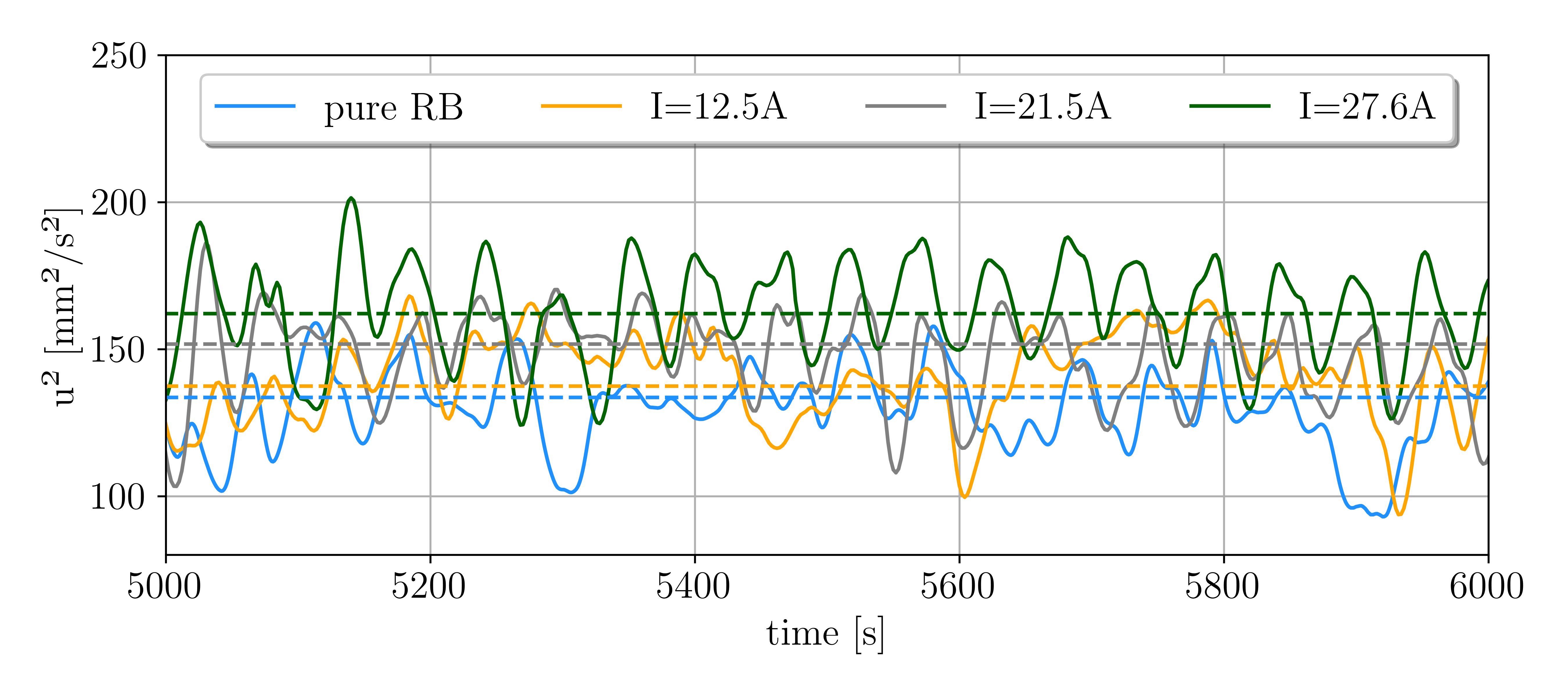
Figure 19: Mean kinetic energy of the flow for the four cases considered in this paper.

As elucidated above, the sharp peak at 18 mHz is proportional to the forcing while being perfectly canceled for the whole volume. It is probably directly driven by the forcing itself. What we are left with at this point is the question about the character of the second frequency which completely dominates the full helicity $H$. This wider frequency bunch still shows natural variation around a center value, suggesting itself as a higher order mode of the slightly more irregular LSC. As is clear from the l.h.s. of Fig. 14 a non-vanishing total $H$ is connected with a typical sloshing motion of the LSC with its $u_{x}$ that is asymmetric in $x$. This was clearly the dominant part for the pure RB case, but evidently some part of it remains also for higher forcing. A natural explanation of the frequency increase, as observed in Fig. 10, would be that the spatial range of the azimuthal LSC’s angle oscillation is restricted by the $m=2$ forcing which dominates the $x$-region farther away from the center. A stronger and more defined helicity oscillation would, in that train of thought, originate from a “stiffer” forcing potential wall. Just as an analogous guitar string would exhibit an increase of eigenfrequency under tension. What is still unexplained then is the sharpness of this second peak as seen in Fig. 16 to Fig. 18 which makes it tempting to speculate about a resonance of higher order (e.g. 4:3 or 3:2), Yet, until now the frequencies shown in Fig. 10 are not really conclusive, so that further work on that issue is definitely required.

IV Conclusions

In this paper we have presented and compared experimental and numerical results on the synchronization of the helicity in a liquid metal RB convection by a time-periodic tide-like force with its typical $m=2$ azimuthal dependence. By increasing the current in the field producing coils, between 10 A and 25 A we have observed a tightening synchronization of the flow by the force. We characterized the typical periods at various locations in the cylinder and found periodic flow structures accordant to the forcing frequency. Surprisingly, we observed also higher frequencies connected with a remaining sidewise motion perpendicular to the main flow direction. We quantified the tightness of synchronicity using a cross correlation method and found strong coherence above a certain threshold. Digging more deeply into the numerical data, helicity synchronization was clearly identified. Above the threshold, the two partial helicities $H^{-}$ and $H^{+}$, left and right of the LSC’s main plane, showed a nearly perfect synchronization with the external frequency, while the full-volume helicity $H$ turned out to have a higher frequency, perhaps related to an odd-numbered synchronization (depending on peak current amplitude), an effect that is still to be understood. For different current strengths, we have visualized the flow which reveals a complicated three-dimensional sloshing motion which acquires, at least partly, also a component that is symmetric with respect to $x$.

Admittedly, the particular final results was slightly against our initial expectation of a rather simple synchronization of the side-wise sloshing motion by the $m=2$ force, allegedly leading to an 1:1 synchronization of the total helicity, too. Such a tidal synchronization of the $m=0$ component of the helicity had been numerically observed for the Tayler instability Weber2015 ; Stefani2016 . The difference to the RB case presented here, with its LSC in form of one single roll, might have to do with the different number of $m=1$ rolls, which was equal to 2 in the TI case (using a slightly taller cylinder). It therefore suggests itself to use also a taller RB flow, with a higher number of rolls stacked above each other Schindler2022 , to better mimick the synchronization of the full-volume helicity as in the TI caseWeber2015 ; Stefani2016 .

Coming back to the motivating subject of a possible synchronization of the helicity in the solar tachocline by planetary tidal forces, it remains to be seen whether the 1:1 synchronized non-axisymmetric helicity component, as observed now, can in any descent way be applied there. At any rate, it would clearly contradict the original idea of a Tayler-Spruit dynamo with axisymmetric helicity distribution. While clearly admitting that the analogy of our RB model with the TI in a thin tachocline should not be overstretched, we also point out that an asymmetric helicity distribution (although with respect to the equator) was at the root of our 1D-synchronization model Stefani2019 of the solar dynamo. Another interesting point might be whether any higher order synchronization, could be helpful for explaining some corresponding periodicities Paula2022 of the solar dynamo.

Conflict of Interest

The authors have no conflicts to disclose.

Data Availability

The data that support the findings of this study are available from the corresponding author upon reasonable request.

Author Contributions

Peter Jüstel: Conceptualization (support), Investigation (equal), Data curation (lead), Formal analysis (lead), Methodology (equal), Visualization (lead), Software (equal), Writing - original draft (equal) Sebastian Röhrborn: Conceptualization (support), Investigation (equal), Data curation (equal), Formal analysis (equal), Methodology (equal), Visualization (equal), Software (equal), Writing - review & editing (equal) Sven Eckert: Supervision (supporting), Methodology (supporting), Writing - review & editing (supporting) Vladimir Galindo: Visualization (supporting), Data Curation (supporting), Formal analysis (supporting), Software (equal), Methodology (supporting), Writing - review & editing (equal) Thomas Gundrum: Investigation (supporting), Software (supporting), Methodology (supporting), Resources, Writing - review & editing (supporting) Rodion Stepanov: Conceptualization (equal), Formal analysis (supporting) Frank Stefani: Conceptualization (lead), Funding acquisition, Methodology (lead), Project administration, Supervision (lead), Visualization (supporting), Writing - original draft (equal)

Appendix

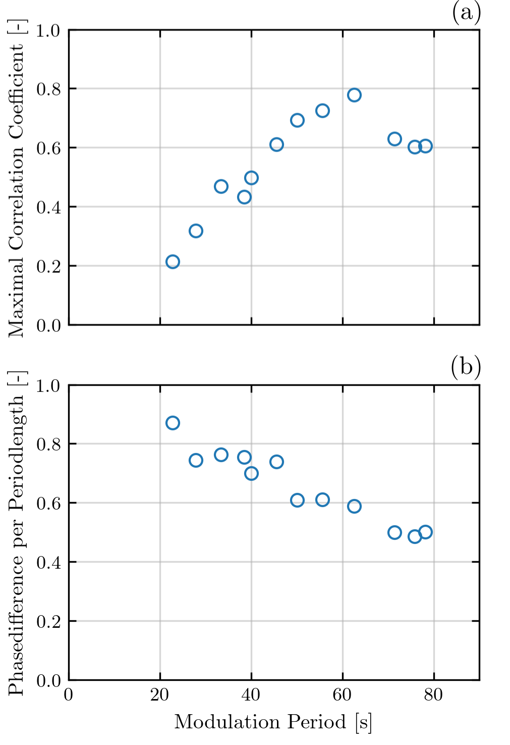
Figure 20: Maximal empirical correlation coefficients of sensor “Bot3” as in Fig. 11 for a fixed maximal current amplitude of 21.2 A and a variation of the modulation frequency. (a) Correlation coefficients (b) Phase difference normalized to the modulation period.

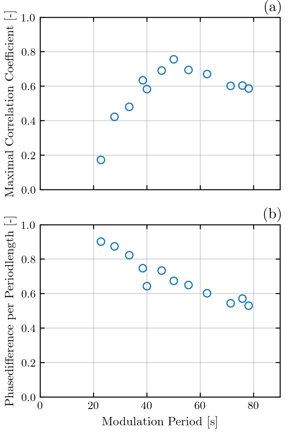
Figure 21: Same as Fig. 20 for “Top3” sensor.

Additionally to the synchronization boundary, a shift in modulation frequencies has been investigated. In Fig. 20 the result is displayed for the “Bot3” sensor. It shows a broad maximum around the LSC’s sloshing period of roughly 55 s. The maximum appears to be at over 60 s, but one has to consider the statistical variance of the values at 21.2 A, as in Fig. 11. This is also emphasized by Fig. 21, where the values for the “Top3” sensor are given. In this case, the maximum is slightly left of 55 s. We interpret these results such that the “resonance” of the forcing with the RB process is strongest at the natural sloshing frequency

The phase difference in panel (b) of Figs. 20 and 21 has been normalized to the length of one period to make the results comparable. Interestingly, the flow’s lag decreases linearly from almost one period at fast modulations to about half a period for slow modulations irrespective of the apparent synchronization strength.

References

- (1) H.K. Moffatt, "Helicity," Comptes Rendus Mecanique , 346, 165 (2018).
- (2) J.B. Taylor, "Relaxation and magnetic reconnection in plasmas," Rev. Mod. Phys. , 58, 741 (1986).
- (3) F. Rincon, "Dynamo theories," J. Plasma Phys., 84, 205850401 (2019).
- (4) S. Tobias, "The turbulent dynamo," J. Fluid Dyn. , 912, P1 (2021).
- (5) F. Stefani, A. Gailitis, and G.Gerbeth, "Magnetohydrodynamic experiments on cosmic magnetic fields," Zeitschr. Angew. Math. Mech., 88, 930 (2008).
- (6) P. Charbonneau, "Dynamo models of the solar cycle," Liv. Rev. Solar Phys. , 17, 4 (2020).
- (7) R.H. Dicke, "Is there a chronometer hidden deep in the Sun?" Nature, 276, 676 (1978).
- (8) H. Vos, C. Brüchmann, A. Lücke, J.F.W. Negendank, G.H. Schleser, B. Zolitschka, "Phase stability of the solar Schwabe cycle in lake Holzmaar, Germany, and GISP2, Greenland, between 10,000 and 9,000 cal. BP." In: Fischer, H., Kumke, T., Lohmann, G., Flöser, G., Miller, H., von Storch, H., Negendank, J.F. (eds.), "The Climate in Historical Times: Towards a Synthesis of Holocene Proxy Data and Climate Models", GKSS School of Environmental Research, Springer, Berlin, 293 (2004).
- (9) F. Stefani, J. Beer, A. Giesecke, T. Gloaguen, M. Seilmayer, R. Stepanov, and T. Weier, "Phase coherence and phase jumps in the Schwabe cycle" Astron. Nachr. 341, 600 (2020).
- (10) C.-C. Hung, "Apparent relations between solar activity and solar tides caused by the planets," NASA/TM-2007-214817 (2007).
- (11) I.R.G. Wilson, "Does a spin-orbit coupling between the Sun and the Jovian planets govern the solar cycle?" Publ. Astron. Soc. Aust. 25, 85 (2008).
- (12) I.R.G. Wilson, "The Venus-Earth-Jupiter spin-orbit coupling model," Pattern Recogn. Phys. 1, 147 (2013).
- (13) N. Scafetta, "Does the Sun work as a nuclear fusion amplifier of planetary tidal forcing? A proposal for a physical mechanism based on the mass-luminosity relation.," J. Atmos. Solar-Terr. Phys. 81-82, 27 (2012).
- (14) N. Weber, V. Galindo, F. Stefani, and T. Weier, "The Tayler instability at low magnetic Prandtl numbers: between chiral symmetry breaking and helicity oscillations," New Journal of Physics, 17, 113013 (2015).
- (15) F. Stefani, A. Giesecke, N. Weber, and T. Weier, "Synchronized helicity oscillations: a link between planetary tides and the solar cycle?" Solar Phys. 291, 2197 (2016).
- (16) F. Stefani, A. Giesecke, and T. Weier, "On the synchronizability of Tayler-Spruit and Babcock-Leighton type dynamos," Sol. Phys. 293, 12 (2018).
- (17) F. Stefani, A. Giesecke, and T. Weier, "A model of a tidally synchronized solar dynamo," Sol. Phys. 294, 60 (2019).
- (18) F. Stefani, A. Giesecke, M. Seilmayer, R. Stepanov, and T. Weier, "Schwabe, Gleissberg, Suess-de Vries: Towards a consistent model of planetary synchronization of solar cycles," Magnetohydrodynamics 56, 269 (2020).
- (19) F. Stefani, R. Stepanov, and T. Weier, "Shaken and stirred: When Bond meets Suess-de Vries and Gnevyshev-Ohl," Solar Phys. 296, 88 (2021).
- (20) R. J. Tayler, "The adiabatic stability of stars containing magnetic fields - I.Toroidal fields," Mon. Not. R. Astron. Soc. 161, 365–380 (1973).
- (21) M. Seilmayer, F. Stefani, T. Gundrum, T. Weier, G. Gerbeth, M. Gellert, and G. Rüdiger, "Experimental evidence for a transient Tayler instability in a cylindrical liquid-metal column," Phys. Rev. Lett. 108, 244501 (2012).
- (22) D.K. Callebaut, C. de Jager, S. Duhau, "The influence of planetary attractions on the solar tachocline," J. Atmos. Sol.-Terr. Phys. 80, 73 (2012).
- (23) P. Charbonneau, "External forcing of the solar dynamo", Front. Astron. Space Sci. 9, 853676 (2022).
- (24) M. Dikpati, P.S. Cally, S.W. McIntosh, and E. Heifetz, "The origin of the "seasons" in space weather," Sci. Rep. 7, 14750 (2017).
- (25) S.W. McIntosh, W.J. Cramer, M. Pichardo Marcano, and R.J. Leamon, "The detection of Rossby-like waves on the Sun," Nature Astron. 11, 0086 (2017).
- (26) X. Márquez-Artavia, C.A. Jones, and S.M. Tobias, "Rotating magnetic shallow water waves and instabilities in a sphere," Geophys. Astrophys. Fluid Dyn. 111, 282 (2017).
- (27) T. Zaqarashvili, "Equatorial magnetohydrodynamic shallow water waves in the solar tachocline," Astron Astrophys. 856, 32 (2018).
- (28) T. Zaqarashvili et al., "Rossby waves in astrophysics," Space Sci. Rev. 217, 15 (2021).
- (29) G.Horstmann, personal communication (2022)
- (30) J. Schumacher and K.R. Sreenivasan, "Colloquium: Unusual dynamics of convection in the Sun," Rev. Mod. Phys. 92 041001, (2020)
- (31) R. Krishnamurti, and L.N. Howard, "Large-scale flow generation in turbulent convection," Proc. Natl. Acad. Sci. 78, 1991 (1981).
- (32) M. Sano, X.-Z. Wu, and A. Libchaber, "Turbulence in helium-gas free convection," Phys. Rev. A 40, 6421 (1989).
- (33) T. Takeshita, T. Segawa, J.A. Glazier, and M. Sano, "Thermal turbulence in mercury," Phys. Rev. Lett. 76, 1465 (1996).
- (34) S. Cioni, S. Ciliberto, and J. Sommeria, "Strongly turbulent Rayleigh-Bénard convection in mercury: comparison with results at moderate Prandtl number," J. Fluid Mech. 335, 111 (1997).
- (35) H.-D. Xi, S. Lam., and K.-Q. Xia, "From laminar plumes to organized flows: the onset of large-scale circulation in turbulent thermal convection," J. Fluid Mech. 503, 47 (2004).
- (36) E. Brown and G. Ahlers, "Rotations and cessations of the large-scale circulation in turbulent Rayleigh-Bénard convection," J. Fluid Mech. 568, 351 (2006).
- (37) C. Resagk, R. du Puits, A. Thess, F.V. Dolzhansky, S. Grossman, F.F. Araujo, and D. Lohse, "Oscillations of the large scale wind in turbulent thermal convection," Phys. Fluids 18, 095105 (2006).
- (38) H.-D. Xi, and K.-Q. Xia, "Cessations and reversals of the large-scale circulation in turbulent thermal convection," Phys. Rev. E 75, 066307 (2008).
- (39) L.P. Kadanoff, "Turbulent heat flow: structure and scaling," Phys. Today 54, 34 (2001).
- (40) D. Funfschilling and G. Ahlers, "Plume motion and large scale circulation in a cylindrical Rayleigh-Bénard cell," Phys. Rev. Lett. 92, 194502 (2004).
- (41) H.-D. Xi, S.-Q. Zhou, T.-S. Chan, and K.-Q. Xia, "Origin of temperature oscillation in turbulent thermal convection," Phys. Rev. Lett. 102, 044503 (2009).
- (42) E. Brown, G. Ahlers, "The origin of oscillations of the large-scale circulation of turbulent Rayleigh-Bénard convection," J. Fluid Mech. 638, 383 (2009).
- (43) R. Khalilov, I. Kolesnichenko, A. Pavlinov, A. Mamykin, and A. Shestakov, "Thermal convection of liquid sodium in inclined cylinders," Phys. Rev. Fluids 3, 043503 (2018).
- (44) T. Wondrak, J. Pal, F. Stefani, V. Galindo, and S. Eckert, "Visualization of the global flow structure in a modified Rayleigh-B énard setup using contactless inductive flow tomography," Flow. Meas. Instrum. 62, 269 (2018).
- (45) T. Zürner, F. Schindler, T. Vogt, S. Eckert, and J. Schumacher, "Flow regimes of Rayleigh-Bénard convection in a vertical magnetic field,", J. Fluid Mech. 894, A21 (2020).
- (46) C. Morize, M. Le Bars, P. Le Gal, and A. Tilgner, "Experimental determination of zonal winds driven by tides,", Phys. Rev. Lett. 104. 214501 (2010)
- (47) R. Stepanov, F. Stefani, "Electromagnetic forcing of a flow with the azimuthal wave number m = 2 in cylindrical geometry", Magnetohydrodynamics 55, No. 1/2, 207-214 (2019).
- (48) P. Jüstel et al., "Generating a tide-like flow in a cylindrical vessel by electromagnetic forcing", Phys. Fluids 32, 097105 (2020).
- (49) S. Röhrborn et al., "Analyzing a modulated electromagnetic forcing and its capability to synchronize the large scale circulation in a Rayleigh-Bénard cell of aspect ratio ," Magnetohydrodynamics 58, 187-193 (2022).
- (50) S. Röhrborn et al., "Numerical simulation of the tidal synchronization of the large-scale circulation in Rayleigh-B’enard convection with aspect ratio 1," Magnetohydrodynamics, in press (2022).
- (51) J. Pal, A. Cramer, T. Gundrum, and G. Gerbeth, "MULTIMAG - A MUL- TIpurpose MAGnetic system for physical modelling in magnetohydrodynamics," Flow Meas. Instr. 20, 241 (2009).
- (52) Y. Plevachuk, V. Sklyarchuk, N. Shevchenko, and S. Eckert, "Electrophysical and structure-sensitive properties of liquid Ga-In alloys," Int. J. Mater. Res. 106, 66 (2015).
- (53) T. Zürner, F. Schindler, T. Vogt, S. Eckert, J. Schumacher, "Combined measurement of velocity and temperature in liquid metal convection," J. Fluid Mech. 87, 1108 (2019).
- (54) OpenCFD, OpenFOAM - The Open Source CFD Toolbox - User’s Guide, OpenCFD Ltd., United Kingdom, 3rd ed. (2015).
- (55) Opera, Opera - Simulation Software (Brochure), ©Dassault Systems, (2018)
- (56) F. Schindler, S. Eckert, T. Zürner, J. Schumacher, and T. Vogt, "Collapse of coherent large scale flow in strongly turbulent liquid metal convection," Phys. Rev. Lett. 128, 164501 (2022).
- (57) V. de Paula, J.J. Curto, and R. Oliver, "The cyclic behaviour in the N-S asymmetry of sunspots and solar plages for the period 1910 to 1937 using data from Ebro catalogues", arXiv:22.02.08628 (2022).