The circumstellar material around the Type IIP SN 2021yja

Abstract

The majority of Type II-plateau supernovae (SNe IIP) have light curves that are not compatible with the explosions of stars in a vacuum; instead, the light curves require the progenitors to be embedded in circumstellar matter (CSM). We report on the successful fitting of the well-observed SN IIP 2021yja as a core-collapse explosion of a massive star with an initial mass of $\sim 15$ $\mathrm{M}_{\odot}$ and a pre-explosion radius of 631 $\mathrm{R}_{\odot}$. To explain the early-time behaviour of the broad-band light curves, the presence of 0.55 $\mathrm{M}_{\odot}$ CSM within $\sim 2\times 10^{\,14}$ cm is needed. Like many other SNe IIP, SN 2021yja exhibits an early-time flux excess including ultraviolet wavelengths. This, together with the short rise time ($<2$ days) in the $gri$ bands, indicates the presence of a compact component in the CSM, essentially adjacent to the progenitor. We discuss the origin of the pre-existing CSM, which is most likely a common property of highly convective red supergiant envelopes. We argue that the difficulty in fitting the entire light curve with one spherical distribution indicates that the CSM around the SN 2021yja progenitor was asymmetric.

1 Introduction

The evidence for exploding massive stars being surrounded by circumstellar matter (CSM) increases with almost each newly discovered Type II-plateau supernova (SN IIP; Yaron et al., 2017; Förster et al., 2018; Morozova et al., 2018; Dessart & Hillier, 2019; Goldberg & Bildsten, 2020; Hiramatsu et al., 2021; Bruch et al., 2021). Up to 70% of SNe IIP cannot be explained by progenitors located in a vacuum, but require the presence of nearby CSM. The CSM may be explained by an extraordinarily strong, steady wind that a massive star experiences during the few years prior to exploding (Smith, 2014). Just before collapse, core silicon burning lasts only a day, and core oxygen burning lasts a year. One could speculate that the claimed wind happens during the last years of core carbon burning and core neon burning. Other possible mechanisms for producing this expulsion of the outermost layers include the $\varepsilon$-mechanism (Morozova et al., 2020; Tinyanont et al., 2022) or gravity/acoustic waves (Fuller, 2017). As we discuss here, yet another option is that the binary undergoes a common-envelope (CE) phase, merges, and ejects a fraction of the CE considered for dense CSM around some extreme SNe by Chevalier (2012). However, we argue that the most natural scenario for SN 2021yja and similar IIP SNe is a globally asymmetric structure of the red supergiant (RSG) and its tenuous atmosphere caused by convective motions.

The recently discovered SN IIP 2021yja (Vasylyev et al., 2022; Hosseinzadeh et al., 2022) shows a blue excess in its spectra at early times. Hosseinzadeh et al. (2022) claim a wind mass-loss rate of $10^{-6}$ $\mathrm{M}_{\odot}$ yr^-1, normal for RSG winds (Goldman et al., 2017; Beasor et al., 2020). In this study we test the hypothesis of the possible presence of matter surrounding SN 2021yja. The reconstructed colour-temperature evolution during the first 20 days shows the decline of $T_{\mathrm{col}}\propto t^{-0.6}$ predicted by shock-cooling models (Nakar & Sari, 2010; Rabinak & Waxman, 2011; Shussman et al., 2016; Faran & Sari, 2019). As suggested by Kozyreva et al. (2020a), the colour temperature during this phase is a good indicator of the progenitor radius; thus, Hosseinzadeh et al. (2022) approximate it to be 900 $\mathrm{R}_{\odot}$ or 2000 $\mathrm{R}_{\odot}$, depending on the assumed shock-cooling model, respectively Shussman et al. (2016) and Sapir & Waxman (2017). As correctly mentioned by Morag et al. (2022), an analytic formulation always provides a very rough estimate and serves as an approximate diagnostic. In fact, Hosseinzadeh et al. (2022) compare the colour-temperature evolution of SN 2021yja to a set of numerical simulations of RSG models. The numerical simulations agree well with the analytic formulation by Shussman et al. (2016), who present updated versions of the formulae by Nakar & Sari (2010). According to Shussman et al. (2016), $T_{\mathrm{col}}\propto R^{\,0.46}\,E^{\,-0.25}$, where $R$ is the progenitor radius and $E$ is an explosion energy. For simplicity, the energy is dropped off in the mentioned comparison, while $E$ is close to 1 foe (1 foe $=10^{51}$ erg) and the dependence on $E$ is weaker than dependence on $R$. If the explosion energy of SN 2021yja differs from 1 foe, the progenitor radius estimate varies accordingly as $R\propto E^{\,0.25/0.46}\approx E^{\,0.54}$ for the same colour temperature. Hence, if the energy is 50% higher then the radius is larger by a factor of 1.3, although it is still a rough estimate. Nevertheless, we emphasise that the inferred CSM/wind is optically thin before the shock propagation and does not affect the estimated progenitor radius (Dessart et al., 2017).

The paper is structured as follows. In Section 2 we describe our two best-fitting models. Section 3 presents our broad-band light curves, which match the observed light curves of SN 2021yja, are presented in Section 3, and in Section 6 we summarise our findings.

2 Input model and Method

We used model m15 from Kozyreva et al. (2019) — namely, the case with a high explosion energy of 1.53 foe. This is a 15 $\mathrm{M}_{\odot}$ solar metallicity stellar evolution model computed with MESA (Paxton et al., 2015) and exploded with V1D (Livne, 1993). We consider two values for the total mass of radioactive nickel: 0.175 $\mathrm{M}_{\odot}$ (model m15ni175) and 0.2 $\mathrm{M}_{\odot}$ (model m15ni2), although Hosseinzadeh et al. (2022) and Vasylyev et al. (2022) claim a ⁵⁶Ni mass of 0.141 $\mathrm{M}_{\odot}$ and 0.2 $\mathrm{M}_{\odot}$, respectively, based on the radioactive tail luminosity. The ⁵⁶Ni mass fraction was scaled to have a total mass of 0.175 $\mathrm{M}_{\odot}$ or 0.2 $\mathrm{M}_{\odot}$ while reducing the mass fraction of silicon. We set the higher mass of ⁵⁶Ni because the tail luminosity is not matched by a model with 0.141 $\mathrm{M}_{\odot}$ of radioactive nickel. 0.2 $\mathrm{M}_{\odot}$ of ⁵⁶Ni is at the upper limit of the total amount of radioactive nickel produced in a neutrino-driven explosion; however, it is still within the range of accepted uncertainties (Ertl et al., 2016; Sukhbold et al., 2016; Ertl et al., 2020). Moreover, if there is any asymmetry in the SN ejecta, the effective $4\pi$-equivalent mass of ⁵⁶Ni might be higher (Kozyreva et al., 2022; Sollerman et al., 2022).

We notice that the shape of the transition from the plateau to the radioactive tail in the bolometric light curve of SN 2021yja is very shallow. This is similar to the light curve of a self-consistent explosion of a 15 $\mathrm{M}_{\odot}$ progenitor and its three-dimensional (3D) post-explosion hydrodynamics simulations carried out with the PROMETHEUS-VERTEX code (Wongwathanarat et al., 2015; Utrobin et al., 2017). In these simulations the SN ejecta undergo strong macroscopic mixing. The iron-group elements, including radioactive nickel, are mixed far beyond the core and penetrate the hydrogen-rich envelope. Conversely, hydrogen is mixed deep into the interior of the SN ejecta. The combination of radioactive nickel mixed thoroughly with hydrogen in the ejecta leads to a shallow and smooth drop from the plateau. Therefore, in our current study we modify model m15 by artificially mixing hydrogen inward. The final chemical composition of model m15ni175 is shown in Figure 1.

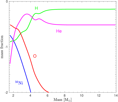
Figure 1: Chemical structure of model m15ni175. We show selected elements: hydrogen (green), helium (magenta), oxygen (red), and radioactive nickel (blue).

As SN 2021yja has a blue excess at early times, Hosseinzadeh et al. (2022) conclude that the progenitor exploded in a pre-existing tenuous environment which the authors call a “weak wind.” This particular wind rate was chosen based on the synthetic observables computed by Dessart et al. (2017). Therefore, we assume the existence of matter around the progenitor. We carried out simulations for a variety of radii, “interface” density of the CSM (the density where the CSM is adjacent to the progenitor), density slopes, and CSM with shells. Here we report only on the most successful models in which the CSM was directly attached to the surface of the progenitor. The density slope was assumed to conform to $\rho\propto r^{-2}$, and the extent of the CSM was chosen to be $1.8\times 10^{\,14}$ cm (2700 $\mathrm{R}_{\odot}$). In total, the CSM mass is 0.55 $\mathrm{M}_{\odot}$. Assuming a wind origin for the CSM, a rough estimate of the wind mass-loss rate is

$$\dot{M}\approx{\Delta M_{\mathrm{wind}}v\over{R}}={(0.55\,\mathrm{M}_{\odot})(20\,\mathrm{km\,s}^{-1})\over{1.8\times 10^{14}\,\mathrm{cm}}}\approx 0.18\,\mathrm{M}_{\odot}\,\mathrm{yr}^{-1}\,,$$ (1)

where we input a typical RSG wind velocity of 20 km s^-1 (Goldman et al., 2017; Beasor & Davies, 2018). We discuss the proposed mass of the CSM material in Section 4. Eight additional models with a variety of CSM configurations are presented in Appendix A.

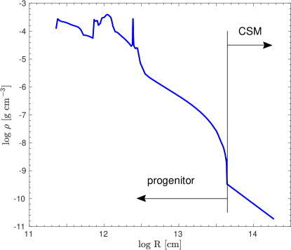
Figure 2: Density structure of model m15ni175.

Models m15ni175 and m15ni2 were mapped into the 1D radiation-hydrodynamics code STELLA (Blinnikov et al., 2006) . STELLA is capable of processing hydrodynamics, including shock propagation and its interaction with the medium, as well as the radiation field evolution — computing light curves, spectral energy distributions, and the resulting broad-band magnitudes and colours. We use the standard parameter settings, well-explained in many papers involving STELLA simulations (see, e.g., Tsvetkov et al., 2021; Moriya et al., 2020). The thermalisation parameter is set to 0.9, as recommended by the recent study of Kozyreva et al. (2020b).

We note that the CSM is added as an attached density profile with the same temperature and chemical composition as the last zone of the progenitor model, and zero velocity artificially. Therefore, the stellar structure with the attached CSM is not in hydrodynamical and thermal equilibrium. Consequently, the radiation field is not fully trustable during roughly the first day. In the plot showing the rising part of the light curve in Section 5, we deliberately do not show the first day of simulations.

3 Results

3.1 Light curve

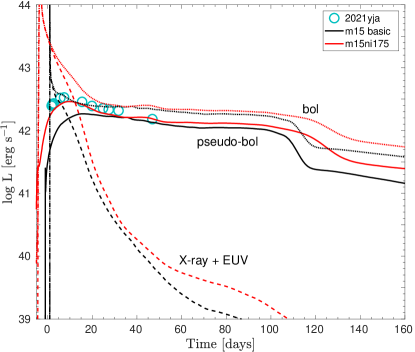
Figure 3: Pseudobolometric (solid), bolometric (dotted), and X-ray-EUV (dashed), light curves for model m15ni175 (red), along with the “bolometric” data of SN 2021yja (circles). We show the basic model m15 in black for reference and to demonstrate the effect of interaction.

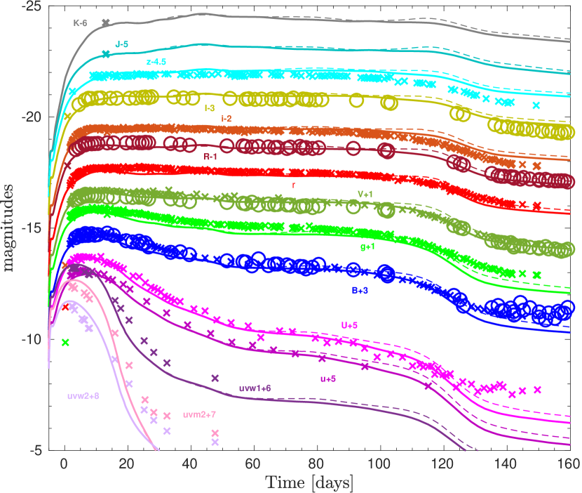
Figure 4: Broad-band light curves for models m15ni175 (thick curves) and m15ni2 (dashed curves), together with SN 2021yja. Crosses represent the observations taken from Hosseinzadeh et al. (2022), and circles represent data taken from Vasylyev et al. (2022). The statistical uncertainties of the observations are smaller than the data points. Time “0” corresponds to the explosion epoch introduced by Hosseinzadeh et al. (2022). The synthetic curves are shifted by $-8$ days to match the early phase and the end of the plateau.

In Figure 3, we present pseudobolometric, bolometric, and X-ray-EUV ($\lambda<325$ Å) light curves for the models m15ni175 (which we call “best-fit” or “best” hereafter), as well as the basic model m15, with the “bolometric” data of SN 2021yja superposed. We note that the synthetic bolometric light curves of our models are truly bolometric, while the “bolometric” light curve of SN 2021yja is not truly bolometric; instead, it is constructed based on photometric data fitted to a blackbody via Markov-Chain-Monte-Carlo light-curve fitting (Hosseinzadeh & Gomez, 2020). In this study, we intend to compare our synthetic observables to the broad-band magnitudes to avoid misinterpretation while comparing to the derived bolometric light curve of SN 2021yja. Figure 3 shows the default progenitor m15 from Kozyreva et al. (2019) as a reference to illustrate the effect of the CSM. The shock propagates through the extended surrounding medium and ionises it, turning it into a hot, expanding, relatively optically thick layer. Later cooling in this tenuous layer is responsible for the high luminosity in bluer bands. We avoid calling this mechanism “interaction” since this is the natural propagation of the shock in the pre-existing CSM adjacent to the progenitor. The difference between the default model m15 and model m15ni175, clearly demonstrates that the presence of an extended medium plays a significant role in shaping the early-time light curve during the first 35 days.

Figure 4 shows the broad-band light curves for our models m15ni175 and m15ni2, together with photometric data SN 2021yja taken from Hosseinzadeh et al. (2022) and Vasylyev et al. (2022). We note that these two observational studies propose two different distance moduli and extinction values, even though the derived absolute magnitudes do not differ significantly. The time “0” is the same as in Hosseinzadeh et al. (2022) — the estimated explosion epoch, which differs from the actual moment of core collapse. The explosion epoch introduced by Hosseinzadeh et al. (2022) is calculated based on the nondetection, the first detection, and the assumed approximation. In nature, the shock breaks out on the progenitor’s surface $\sim 1$ day after the actual explosion, if the progenitor is located in a vacuum (for the basic model), and becomes “visible”. In the case when the progenitor is embedded in the CSM (e.g., in the best-fit model), the shock breaks out after 4 days at the edge of the CSM. Hence, the explosion epoch in Figure 4 is not the same as the actual moment of core collapse, because there is a time lapse until the explosion becomes “visible”, and there is some relative degree of freedom to set the time shift for the synthetic curves. The light curves of SN 2021yaj in the majority of broad bands ($U\!V\!W\!1$, $U\!V\!M\!2$, $U\!V\!W\!2$, $uU\!BgV\!rRiIzJK$) are matched by our synthetic light curves well during the entire observed period. We show models with two different masses of radioactive nickel, since in some broad bands on the tail the model with 0.2 $\mathrm{M}_{\odot}$ of nickel fits the data better. There is some disagreement in the $U$ and $z$ bands at later times, after day 130, when the ejecta become more transparent, and proper spectral synthesis is required.

Our best-fit models do not match the first data points collected in the $gri$ bands at day 0.225 with the MuSCAT3 instrument. We discuss a possible solution for this tension in Section 5 while introducing a model with the CSM having a different density profile. The synthetic light curves in the UV bands $U\!V\!W\!1$, $U\!V\!M\!2$, and $U\!V\!W\!2$ also reproduce the observed magnitudes reasonably well, although they slightly overestimate the flux during the first 10 days, and underestimate the flux after day 20. The same model introduced to match the first $gri$ points with the different CSM density gradient fits the UV bands better for the earlier epoch. Hence, we assume that SN 2021yja might have CSM with asymmetric density structure.

3.2 Photospheric velocity

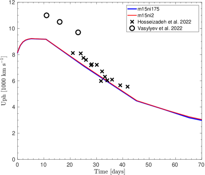
Figure 5: Photospheric velocity evolution for models m15ni175 and m15ni2, and for SN 2021yja. Crosses represent velocities obtained from fits to the iron line in Hosseinzadeh et al. (2022), and circles represent velocities from spectral modelling in Vasylyev et al. (2022).

In Figure 5, we present the synthetic photospheric velocity evolution derived from the location of the photosphere in the $B$ band (where the integrated optical depth in $B$ equals 2/3) and the photospheric velocity evolution of SN 2021yja. The data taken from Vasylyev et al. (2022) are derived via spectral modelling, while the data taken from Hosseinzadeh et al. (2022) are derived via the absorption minimum of the P Cygni profile of spectral line Fe II $\lambda 5169$. The agreement between our prediction and the velocity estimate from the iron line is very satisfactory. However, our models do not explain the velocity estimate derived from the spectral modelling, though this is to some extent model-dependent and should be considered with caution. For example, there is the epoch at day 20–21 when the photospheric velocity is estimated by both methods — TARDIS spectral modelling and via the iron line. The resulting values are different: 9700 km s^-1 and 8100 km s^-1, respectively. The photospheric velocities estimated via TARDIS modelling are systematically overestimate by 10–20% relative to those calculated via Fe or Sc lines. The estimates for SN 2005cs and SN 1999em (Figure 11, Vasylyev et al., 2022) give 4000–4500 km s^-1 (day 15) and 6000 km s^-1 (day 30), respectively, while using TARDIS spectral modelling methodology. On the contrary, Pastorello et al. (2009) estimate velocities of 3400–3800 km s^-1 for SN 2005cs and 5500 km s^-1 for SN 1999em at the same epochs via spectral lines.

Overall, the broad-band light curves and photospheric-velocity evolution are matched reasonably well with our modified 15 $\mathrm{M}_{\odot}$ stellar model embedded in confined CSM. This agrees with findings by Vasylyev et al. (2022), who reported a possible 15 $\mathrm{M}_{\odot}$ progenitors based on the analysis of archival Hubble Space Telescope data.

4 Possible origin of the CSM

The amount of CSM required by matching the light curves of SN 2021yja is 0.55 $\mathrm{M}_{\odot}$. Assuming that the CSM was produced by a steady wind, the corresponding wind estimate is 0.18 $\mathrm{M}_{\odot}$ yr^-1 (see Eq. 1), which is extraordinarily high and cannot be explained by a normal, steady, RSG wind mass-loss rate. However, the mass of CSM defined by our simulations is in good agreement with estimates done for other SNe IIP (Morozova et al., 2018; Goldberg & Bildsten, 2020). Below we discuss a few possible origins for the pre-existing CSM.

4.1 Binary interaction

Let us consider that the progenitor is a member of a binary system and that the CSM originates from recent mass-transfer interaction. The best-fitting model requires that $\sim 0.55$ $\mathrm{M}_{\odot}$ of matter is ejected on a short timescale of just a few years. This is much more than could be lost from a binary as a result of any stable (nondynamical) mass transfer; a typical rate of thermal-timescale mass transfer is $\sim 10^{-3}$–$10^{-2}$ $\mathrm{M}_{\odot}$ yr^-1. Instead, a feasible possibility is mass transfer that becomes dynamically unstable, leading to CE inspiral and a stellar merger, during which a portion of the RSG envelope may become unbound (e.g., Podsiadlowski, 2001; Morris & Podsiadlowski, 2006; Ivanova et al., 2020). The onset of the CE would have to be rapid in order to prevent significant pre-CE mass loss from the L2 and L3 points (Pejcha, 2014; Pejcha et al., 2017; MacLeod & Loeb, 2020; Blagorodnova et al., 2021) that would extend the CSM to larger radii ($\sim 10^{15}$–$10^{16}$ cm). This could be achieved through Darwin instability (Darwin, 1879), granted that the companion is $\gtrsim 6$ times less massive than the RSG (Fig. 8 in MacLeod et al., 2017, assuming $\eta_{1}\approx 0.15$ typical for RSGs). Given the low binding energies of RSG envelopes (Klencki et al., 2021), even such a low-mass companion could generate enough energy during a CE inspiral to eject $\gtrsim 0.5$ $\mathrm{M}_{\odot}$ of matter. This scenario, although in principle viable, is however extremely rare, as it would require the mass-transfer interaction to occur just a few years before core collapse. In Appendix A, based on 1D stellar models of radial expansion of RSGs, we estimate the rate of such events as $\lesssim 10^{-4}$ of all SNe, occurring preferentially at very low metallicities of a few percent of $Z_{\odot}$. We note that mass transfer close to core collapse is much more likely in the case of Type Ib or Ic SNe, particularly at low metallicity, where the previously (partially) stripped helium star is expanding during advanced burning, leading to another interaction (Dewi et al., 2002; Laplace et al., 2020; Klencki et al., 2022).

A more likely signature of a recent mass-transfer event is extended CSM at a radial distance $\sim 10$–100 times the size of the primary. Unstable but also stable and nonconservative mass transfer can lead to slow outflows of mass from the system, most likely concentrated in the equatorial plane. Moving at $\sim 20$ km s^-1, such slow ejecta would need $\sim 200$ yr to reach $10^{16}$ cm, making the time window for the onset of mass transfer much wider. Mass-transfer events occurring thousands of years prior to core collapse may still contribute to the CSM at the moment of explosion in the form of a circumbinary disk that remains from the original interaction (Kashi & Soker, 2011; Pejcha et al., 2016). Motivated by this, in Appendix B we test additional progenitor models with a more-extended CSM and shells. In particular, we constructed models with the CSM extending to radii of up to 143,000 $\mathrm{R}_{\odot}$ ($10^{16}$ cm) and having a mass of 0.05 Msun, as well as a model with the same CSM profile and a 0.16 $\mathrm{M}_{\odot}$ shell inserted at the edge of the CSM. The results of radiative-transfer simulations for these cases are presented in Appendix B together with other attempts. The light curve for the model with the shell at a distance of 143,000 $\mathrm{R}_{\odot}$ has two distinct maxima, which are not observed in SN 2021yja. Moreover, the actual interaction leads to distinct spectroscopic signatures — narrow lines, which are also not observed in SN 2021yja. Therefore, this experiment illustrates that the observables of SN 2021yja cannot be reproduced by a model with a shell; thus, binary interaction is unlikely to have played a role in shaping the CSM around SN 2021yja.

4.2 Convective nature of the RSG atmospheres

Studies by Chiavassa et al. (2009), Chiavassa et al. (2011a), Goldberg et al. (2022a) and others show that an RSG has a convective envelope, with a characteristic size of the convective cell on the order of the size of the star itself (up to $\sim 1000$ $\mathrm{R}_{\odot}$; e.g., van Belle et al. 1999; Cruzalèbes et al. 2013; Arroyo-Torres et al. 2014). Convection is inferred from giant structures observed at the stellar surface, with sizes comparable to the stellar radius and evolving on weekly or yearly timescales (e.g., Chiavassa et al., 2010a, 2011b; Montargès et al., 2018; Paladini et al., 2018). This results in extreme atmospheric conditions with large variations in velocity, density, and temperature producing strong radiative shocks in their extended atmosphere that can cause the gas to levitate and thus contribute to mass loss (Freytag et al., 2017; Chiavassa et al., 2011a). We note that the stellar radius is defined as a surface where the integrated Rosseland mean depth equals unity. This means that there is some amount of gravitationally bound stellar matter beyond the optical depth of unity (Kravchenko et al., 2019), which can be swept to a distance of 1500 $\mathrm{R}_{\odot}$ or more. The asymmetry of extended material is not a unique property of an RSG. Oblate extended atmospheres were observed in nearby RSGs such as VX Sagittarii (Chiavassa et al., 2010b, 2022), Betelgeuse (Haubois et al., 2009; Montargès et al., 2021), CE Tauri (Montargès et al., 2018), AZ Cygni (Norris et al., 2021), V602 Carinae (Climent et al., 2020), V766 Centauri (Wittkowski et al., 2017), VY CMa (Kamiński, 2019), and yellow hypergiant IRC$+$10420 (Koumpia et al., 2022). This kind of star being part of a close binary is likely to change its shape according to the equipotential surfaces (the Roche-lobe surface is the critical equipotential surface having the Lagrange point L1), which breaks spherical symmetry.

Therefore, we conclude that our best-fit model which matches the observational properties of SN 2021yja might be explained by a normal RSG star with an asymmetric, extended, convective envelope which is also most likely part of an interacting binary system. It might also be possible that the high-entropy plume was expelled during the last stages of evolution (e.g., hundreds to thousands of years prior the core collapse) and was pointed at the direction close to the line of sight of the Earth. The probable asymmetry is also supported by spectropolarimetric observations of SN 2021yja, which suggest a noticable degree of polarization (Vasylyev et al., in preparation).

5 The constraint from the rise time as a signature of asymmetry

The high-cadence observations by Hosseinzadeh et al. (2022) include a nondetection limit up to $-3$ hr before the estimated explosion epoch and the first detection at day 0.225. Together with the subsequent observations, SN 2021yja shows a feature common to many SNe IIP: a very sharp rise to maximum brightness (e.g., González-Gaitán et al., 2015). The data in the $gri$ bands are incompatible with our best-fit model, which overestimates the flux at this epoch. In Figure 4, the synthetic light curves are shifted to match the $U$-band maximum, the rising phase in the $BV\!g$ bands, and the transition from the plateau to the tail, although the early-time data in the $gri$ bands are not matched (exhibiting a sharp rise of 5.5 mag between day 0.225 and day 1.7). Therefore, we consider an additional model to match these data points. We built a model “sharp” with a sharper density gradient, with slope $\alpha=\Delta\,{\rm log}\,\rho/\Delta\,{\rm log}\,r=-7$ versus $\alpha=-2$ in the best-fit model, and the same CSM extension, $R_{\mathrm{out}}=1.8\times 10^{\,14}$ cm (2700 $\mathrm{R}_{\odot}$; see Fig. 6). The mass of the CSM in the model “sharp” is 0.26 $\mathrm{M}_{\odot}$. The radiative-transfer simulations for this model result in light curves which have shorter rise times, as seen in Figure 7. We present $gri$ light curves for the “sharp” model (together with the “best” model) in Figure 7 which match the first detection data points. Additionally, we show the light curve in the $U$ broad band and in the $U\!V\!W\!1$ band. The $U\!V\!W\!1$ light curve of the “sharp” model fits the Swift data better than the “best” model, even though it slightly underestimates the flux during the first two days, similarly to other bands.

To match the first data points, the best-model “best” and the model “sharp” with the sharper CSM have different shifts in time, a 1.6 day difference. We note that in Figure 7 the best-fit model is shifted by 2.8 days, while in Figure 4 the light curves are shifted by 8 days relative to the explosion in the simulations. Indeed, the shift in time cannot be arbitrary; we choose the different shifts to match the data in broad bands. As discussed in the previous section, RSG envelopes have a highly convective nature (i.e., macroscopic plumes). The 3D structure of the modelled RSG envelope (Goldberg et al., 2022a) shows scatter at a fixed radius coordinate within 1–2 orders of magnitude, which in turn means a scatter in the sound speed in various radial directions and different shock-crossing times. The shock propagates in different radial directions with different speeds and reaches the corrugated photosphere at different times (Chiavassa et al., 2011a; Goldberg et al., 2022b). As both our models are computed with a 1D radiation-transfer code, we do not account for different density structures of the progenitor envelope; therefore, there is physically consistent freedom to apply a relative shift to one of two light curves. Our model “sharp” does not perfectly match the rise, but we show the tendency of the actual progenitor plus CSM system.

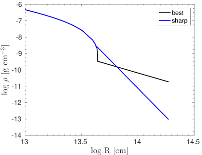
Figure 6: Density structures of the best-fit (“best”) model and the model with the sharper density gradient in the CSM (“sharp”).

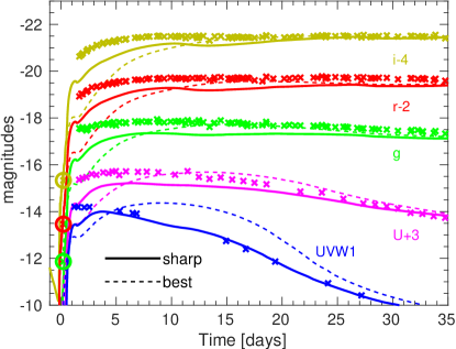
Figure 7: $U\!V\!W\!1$ and $U\!gri$ broad-band magnitudes for the best-fit model “best” (dashed curves) and the model “sharp” with the compact CSM (solid curves), and SN 2021yja.

Hence, we suggest the following physical picture underlying SN 2021yja. The progenitor of SN 2021yja is consistent with our simulations based on an initially 15 $\mathrm{M}_{\odot}$ stellar model with the convective envelope and asymmetric CSM caused by the dynamical nature of the convective envelope. The explosion forms a shock propagating nonspherically within the envelope and breaking at the surface within a day or so. The CSM caused by the plume expulsion forms an asymmetric density structures surrounding the progenitor. The sharp rise time of about 7 days is explained by the model with the sharp density gradient — that is, the first light comes from the radiation front in the radial direction of the compact CSM, while the major fraction of the light curve is then overwhelmed by radiation from the radial directions where the density decline is shallower. The fact that the best-fit model (with the shallower CSM) matches the overall broad-band light curves reasonably well (assuming different time shift; see Fig. 4) offers support for our interpretation.

6 Summary and conclusions

We simulated and explained the broad-band light curves and photospheric-velocity evolution of the bright Type IIP SN 2021yja, which shows an early UV excess. The best-fit models are initially 15 $\mathrm{M}_{\odot}$ RSGs with an admixture of 0.175 $\mathrm{M}_{\odot}$ and 0.2 $\mathrm{M}_{\odot}$ of radioactive ⁵⁶Ni. Light-curve modelling demonstrates the necessity of a high degree of mixing in the post-explosion SN ejecta: outward mixing of radioactive material and inward mixing of hydrogen, which combine to provide a smooth transition from the plateau to the tail. The early-time light-curve evolution is explained by the presence of 0.55 $\mathrm{M}_{\odot}$ of CSM adjacent to the progenitor. The CSM might originate from an asymmetric, convective mass ejection shortly before core collapse, pointing toward the observer. The amount of CSM and radioactive nickel in the ejecta might be lower than in our model, after proper accounting for the asymmetry.

SN 2021yja is another example of an SN IIP that requires CSM to explain the behaviour of early-time light curves. Overall, SNe IIP constitute a large, diverse group of explosions of RSGs surrounded by CSM at various distances, some essentially attached to the star. Analysis of the mass and extension of the CSM in these events will help provide a better understanding of the evolution of massive stars.

We thank Avishay Gal-Yam, Christian Vogl, Stefan Taubenberger, Sergey Blinnikov, Marat Potashov, Sergey Bykov, and Patrick Neunteufel for fruitful discussions, and Griffin Hosseinzadeh and Sergiy Vasylyev for providing the data for SN 2021yja. J.K. acknowledges support from an ESO Fellowship. P.B. is sponsored by grant RFBR 21-52-12032 in his work on the STELLA code development. A.V.F. received funding from the Christopher R. Redlich Fund, numerous individual donors, and Hubble Space Telescope grant GO-16178 from the Space Telescope Science Institute (STScI), which is operated by the Association of Universities for Research in Astronomy (AURA), Inc., under NASA contract NAS5-26555.

Data availability

The data computed and analysed for the current study are available via the link https://wwwmpa.mpa-garching.mpg.de/ccsnarchive/.

Appendix A Details about Probability of CEE

Here we estimate what fraction of all SN progenitors are primary stars in binary systems which engaged in a mass-transfer phase just $\Delta t_{\rm RLOF-CC}$ yr before core collapse. Because we are interested in SN progenitors that explode as RSGs and have most of their envelope retained at the time of core collapse, we only consider the first-ever mass-transfer event from the progenitor (more generally, a component of a binary system can undergo several distinct phases of mass transfer). This allows us to use single stellar models from Klencki et al. (2020) to approximate the evolution of the primary. We assume that the companion is $q=1/10$ of the initial (zero-age) mass of the primary.

For each evolutionary step, we calculate what would need to be the initial orbital period of the binary for the mass transfer to start at that particular $\Delta t_{\rm RLOF-CC}$. Orbital evolution owing to wind mass loss is taken into account. We note that an onset of mass transfer is generally only possible in phases of radial expansion of the primary. We convolve the obtained orbital periods with the initial orbital period distribution of massive binaries, ${\rm d}N/{\rm d\,log}P_{\rm ini}\propto{\rm log}\,P_{\rm ini}^{-0.55}$ (Sana et al., 2012), normalised to the range ${\rm log}\,P_{\rm ini}=[0.15,5.5]$. This allows us to obtain the cumulative distribution of ${\rm log}\,(\Delta t_{\rm RLOF-CC}$ yr^-1), shown in Figure 8 for a primary with 20 $\mathrm{M}_{\odot}$ and several different metallicities. The distribution goes up to $\sim 0.7$ as the remaining $\sim 30\%$ are members of wide noninteracting binaries. We tested that different values of $q$ have negligible effect on the distribution. For the range of interest ${\rm log}\,(\Delta t_{\rm RLOF-CC}$ yr^-1) $\lesssim 4$, there is little effect of changing the primary mass as well.

Figure 8 demonstrates that only about one in every 10,000 SN progenitors is expected to be a primary in a binary system that had undergone its first phase of mass transfer in the last $\lesssim 10$ yr. Figure 8 also gives preference to low-metallicity progenitors ($Z<0.1\,{\rm Z}_{\odot}$), as the higher-metallicity RSG models from Klencki et al. (2020) do not expand during the final evolutionary stages owing to mass loss. We caution, however, that this result is highly uncertain in 1D stellar models. In any case, unless a physical mechanism unaccounted for in the hydrostatic 1D stellar models could cause a significant expansion of RSGs just years prior to core collapse, it is very unlikely for such a SN progenitor to experience mass transfer shortly before the explosion.

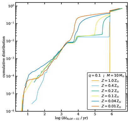
Figure 8: Cumulative distribution of the time between the onset of mass transfer and core collapse, ${\rm log}\,(\Delta t_{\rm RLOF-CC}$ yr${}^{-1})$, estimated for a 20 $\mathrm{M}_{\odot}$ RSG progenitor evolving in a binary with a 1/10 as massive companion, shown for different metallicities.

Appendix B Additional models with Different CSM Structures

We computed additional sets of models to test the effect of more extended CSM, lower density CSM, and CSM in a shell. For this purpose, we constructed models based on the best-fit progenitor model from the main study, and attached different modified CSM distributions instead of the CSM profile used as the best-fit model for SN 2021yja.

Two classes of profiles represent (1) different kinds of extended material with a varied CSM density and radius, and (2) CSM with imitated shells. While the first class might be considered as a steady wind and the extension of the convective plumes of RSGs, the cases with shells might be connected to either eruptive wind mass loss, CE ejection, or any kind of interaction in a close binary system.

The models “reduced $\rho$ 1” and “reduced $\rho$ 2” are shown in dark grey and light grey in Figures 9 and 10. The lower density (factors of 10 and 100 lower than the best-fit model) for the same extension of CSM leads to a lower flux in the early-time bolometric light curves. For the “reduced $\rho$ 2” model the bolometric light curve is very close to the basic progenitor model without CSM (see Fig. 3).

The more extended model “extended 1” with the same “interface” density (density where the CSM is attached to the progenitor) but larger outer radius (almost three times larger) tend to gain higher mass (1.95,$\mathrm{M}_{\odot}$ vs. 0.55 $\mathrm{M}_{\odot}$); consequently, the shock breakout in the CSM is delayed and the bolometric light curve is broader (the dashed black lines in Fig. 10). The $U$-band light curve of the more extended model “extended 1” has a factor of two longer duration and is 0.5 mag brighter. $V$-band magnitude for the extended model “extended 1” is brighter than the best-fit model, and its plateau is affected during the entire duration by the presence of the additional matter. The extended models “extended 2” and “extended 3” (represented by cyan and blue in the figure) have the same “interface” density (a factor of 1000 lower than in the best-fit model), and different extension of 30,000 $\mathrm{R}_{\odot}$ and 143,000 $\mathrm{R}_{\odot}$, respectively. Both “extended 2” and “extended 3” are affected only during the first 20 days (see the bolometric light curves). For the more extended case (“extended 3”), the shock breaks at lower luminosity and a has slower decline, consistent with the shock-cooling models. The broad-band light curves are very similar to those of “extended 1” — even the $U$-band magnitude, which is usually the most sensitive to any changes in the density structure and composition of the SN ejecta.

The cases “Shell 1,” “Shell 2,” and “Shell 3” (magenta, red, and green) show very distinct behaviour of their light curves. All three cases have two maxima; however, “Shell 2” has two maxima merged into one. The first peak represents the shock breakout at the edge of the CSM including the shell, and the second peak is the reproduced energy from the shock passage in the shell. “Shell 1” and “Shell 2” are inserted with the same CSM density profile, although their masses differ significantly (0.03 $\mathrm{M}_{\odot}$ and 0.17 $\mathrm{M}_{\odot}$, respectively). The first maximum in the “Shell 2” model has a lower luminosity because of the larger mass involved. The second maxima in both “Shell 1” and “Shell 2” have similar shape (as the density structures have similar shape but differ in amplitude). The larger the mass in the shell, the longer and the brighter is the second maximum, which is the release of thermal energy after the shock passage. The model “Shell 3” has the shell localed at a larger distance; consequently, both maxima are delayed. Surprisingly, the first maximum of the “Shell 3” case is similar in duration and luminosity to the best-fit model in broad bands, even though the flux is distributed differently, and “Shell 3” has larger red flux ($R$ band) and lower blue flux ($U$ band) than the “best” case. The second maximum occurs at significantly later times, 50 days later than in the “Shell 1” and “Shell 2” cases. This is explained by the lower density (more than 10 times lower in“Shell 3”) and larger radius (a factor of 10 larger in “Shell 3”), which slows the cooling processes in the ionised medium. Maybe some configuration can be found to mimic the best-fit observables, but it is beyond the scope of this paper.

Table 1: Physical properties of the CSM surrounding the best-fit progenitor model used in the current study.

	$\rho_{0}/\rho_{\mathrm{out}}$ [g cm${}^{\,-3}$]	$R_{\mathrm{out}}$ [cm/$\mathrm{R}_{\odot}$]	$M_{\mathrm{CSM}}$ [$\mathrm{M}_{\odot}$]	$M_{\mathrm{shell}}$ [$\mathrm{M}_{\odot}$]
best	$3\times 10^{\,-10}/1.9\times 10^{\,-11}$	$1.9\times 10^{\,14}$/2,700	0.55	0
extended 1	$3\times 10^{\,-10}/2.1\times 10^{\,-12}$	$5.5\times 10^{\,14}$/7,900	1.95	0
reduced $\rho$ 1	$3.8\times 10^{\,-11}/1.8\times 10^{\,-12}$	$1.9\times 10^{\,14}$/2,700	0.055	0
reduced $\rho$ 2	$3.8\times 10^{\,-12}/1.8\times 10^{\,-13}$	$1.9\times 10^{\,14}$/2,700	0.0056	0
extended 2	$3\times 10^{\,-13}/1.9\times 10^{\,-16}$	$2\times 10^{\,15}$/30,000	0.047	0
Shell 1	$3\times 10^{\,-13}/1.9\times 10^{\,-16}$	$2\times 10^{\,15}$/30,000	0.047	0.035
Shell 2	$3\times 10^{\,-13}/1.9\times 10^{\,-16}$	$2\times 10^{\,15}$/30,000	0.047	0.175
extended 3	$3\times 10^{\,-13}/8.3\times 10^{\,-18}$	$1\times 10^{\,16}$/143,000	0.045	0
Shell 3	$3\times 10^{\,-13}/8.3\times 10^{\,-18}$	$1\times 10^{\,16}$/143,000	0.045	0.16

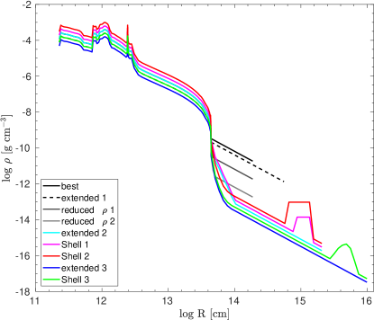
Figure 9: Density structures of the models with CSM structures specified in Table 1. The profiles of the models “extended 1” ($-0.2$), “extended 3” ($-0.4$), “Shell 1” ($+0.2$), “Shell 2” ($+0.4$), and “Shell 3” ($-0.2$) are shown with different offsets (specified in parentheses) for clarity.

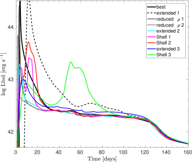
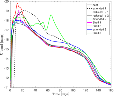
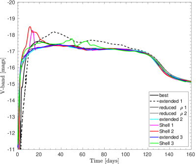
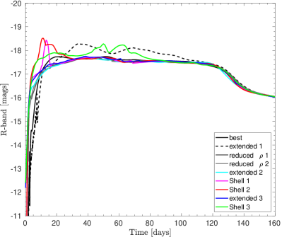
Figure 10: Bolometric, $U$, $V$, and $R$ light curves for the models in Table 1 and in Figure 9. The colours represent the same models as in Figure 9.

References

- Arroyo-Torres et al. (2014) Arroyo-Torres, B., Martí-Vidal, I., Marcaide, J. M., et al. 2014, A&A, 566, A88, doi: 10.1051/0004-6361/201323264
- Beasor & Davies (2018) Beasor, E. R., & Davies, B. 2018, MNRAS, 475, 55, doi: 10.1093/mnras/stx3174
- Beasor et al. (2020) Beasor, E. R., Davies, B., Smith, N., et al. 2020, MNRAS, 492, 5994, doi: 10.1093/mnras/staa255
- Blagorodnova et al. (2021) Blagorodnova, N., Klencki, J., Pejcha, O., et al. 2021, A&A, 653, A134, doi: 10.1051/0004-6361/202140525
- Blinnikov et al. (2006) Blinnikov, S. I., Röpke, F. K., Sorokina, E. I., et al. 2006, A&A, 453, 229, doi: 10.1051/0004-6361:20054594
- Bruch et al. (2021) Bruch, R. J., Gal-Yam, A., Schulze, S., et al. 2021, ApJ, 912, 46, doi: 10.3847/1538-4357/abef05
- Chevalier (2012) Chevalier, R. A. 2012, ApJ, 752, L2, doi: 10.1088/2041-8205/752/1/L2
- Chiavassa et al. (2011a) Chiavassa, A., Freytag, B., Masseron, T., & Plez, B. 2011a, A&A, 535, A22, doi: 10.1051/0004-6361/201117463
- Chiavassa et al. (2010a) Chiavassa, A., Haubois, X., Young, J. S., et al. 2010a, A&A, 515, A12, doi: 10.1051/0004-6361/200913907
- Chiavassa et al. (2009) Chiavassa, A., Plez, B., Josselin, E., & Freytag, B. 2009, A&A, 506, 1351, doi: 10.1051/0004-6361/200911780
- Chiavassa et al. (2010b) Chiavassa, A., Lacour, S., Millour, F., et al. 2010b, A&A, 511, A51, doi: 10.1051/0004-6361/200913288
- Chiavassa et al. (2011b) Chiavassa, A., Pasquato, E., Jorissen, A., et al. 2011b, A&A, 528, A120, doi: 10.1051/0004-6361/201015768
- Chiavassa et al. (2022) Chiavassa, A., Kravchenko, K., Montargès, M., et al. 2022, A&A, 658, A185, doi: 10.1051/0004-6361/202142514
- Climent et al. (2020) Climent, J. B., Wittkowski, M., Chiavassa, A., et al. 2020, A&A, 635, A160, doi: 10.1051/0004-6361/201936734
- Cruzalèbes et al. (2013) Cruzalèbes, P., Jorissen, A., Rabbia, Y., et al. 2013, MNRAS, 434, 437, doi: 10.1093/mnras/stt1037
- Darwin (1879) Darwin, G. H. 1879, Proceedings of the Royal Society of London Series I, 29, 168
- De Beck et al. (2010) De Beck, E., Decin, L., de Koter, A., et al. 2010, A&A, 523, A18, doi: 10.1051/0004-6361/200913771
- Dessart & Hillier (2019) Dessart, L., & Hillier, D. J. 2019, A&A, 625, A9, doi: 10.1051/0004-6361/201834732
- Dessart et al. (2017) Dessart, L., John Hillier, D., & Audit, E. 2017, A&A, 605, A83, doi: 10.1051/0004-6361/201730942
- Dewi et al. (2002) Dewi, J. D. M., Pols, O. R., Savonije, G. J., & van den Heuvel, E. P. J. 2002, MNRAS, 331, 1027, doi: 10.1046/j.1365-8711.2002.05257.x
- Ertl et al. (2016) Ertl, T., Janka, H. T., Woosley, S. E., Sukhbold, T., & Ugliano, M. 2016, ApJ, 818, 124, doi: 10.3847/0004-637X/818/2/124
- Ertl et al. (2020) Ertl, T., Woosley, S. E., Sukhbold, T., & Janka, H. T. 2020, ApJ, 890, 51, doi: 10.3847/1538-4357/ab6458
- Faran & Sari (2019) Faran, T., & Sari, R. 2019, ApJ, 884, 41, doi: 10.3847/1538-4357/ab3e3d
- Förster et al. (2018) Förster, F., Moriya, T. J., Maureira, J. C., et al. 2018, Nature Astronomy, 2, 808, doi: 10.1038/s41550-018-0563-4
- Freytag et al. (2017) Freytag, B., Liljegren, S., & Höfner, S. 2017, A&A, 600, A137, doi: 10.1051/0004-6361/201629594
- Fuller (2017) Fuller, J. 2017, MNRAS, 470, 1642, doi: 10.1093/mnras/stx1314
- Goldberg & Bildsten (2020) Goldberg, J. A., & Bildsten, L. 2020, ApJ, 895, L45, doi: 10.3847/2041-8213/ab9300
- Goldberg et al. (2022a) Goldberg, J. A., Jiang, Y.-F., & Bildsten, L. 2022a, ApJ, 929, 156, doi: 10.3847/1538-4357/ac5ab3
- Goldberg et al. (2022b) Goldberg, J. A., Jiang, Y.-f., & Bildsten, L. 2022b, arXiv e-prints, arXiv:2206.04134. https://arxiv.org/abs/2206.04134
- Goldman et al. (2017) Goldman, S. R., van Loon, J. T., Zijlstra, A. A., et al. 2017, MNRAS, 465, 403, doi: 10.1093/mnras/stw2708
- González-Gaitán et al. (2015) González-Gaitán, S., Tominaga, N., Molina, J., et al. 2015, MNRAS, 451, 2212, doi: 10.1093/mnras/stv1097
- Haubois et al. (2009) Haubois, X., Perrin, G., Lacour, S., et al. 2009, A&A, 508, 923, doi: 10.1051/0004-6361/200912927
- Hiramatsu et al. (2021) Hiramatsu, D., Howell, D. A., Van Dyk, S. D., et al. 2021, Nature Astronomy, 5, 903, doi: 10.1038/s41550-021-01384-2
- Hosseinzadeh & Gomez (2020) Hosseinzadeh, G., & Gomez, S. 2020, Light Curve Fitting, v0.2.0, Zenodo, Zenodo, doi: 10.5281/zenodo.4312178
- Hosseinzadeh et al. (2022) Hosseinzadeh, G., Kilpatrick, C. D., Dong, Y., et al. 2022, arXiv e-prints, arXiv:2203.08155. https://arxiv.org/abs/2203.08155
- Ivanova et al. (2020) Ivanova, N., Justham, S., & Ricker, P. 2020, Common Envelope Evolution, doi: 10.1088/2514-3433/abb6f0
- Kamiński (2019) Kamiński, T. 2019, A&A, 627, A114, doi: 10.1051/0004-6361/201935408
- Kashi & Soker (2011) Kashi, A., & Soker, N. 2011, MNRAS, 417, 1466, doi: 10.1111/j.1365-2966.2011.19361.x
- Klencki et al. (2022) Klencki, J., Istrate, A., Nelemans, G., & Pols, O. 2022, A&A, 662, A56, doi: 10.1051/0004-6361/202142701
- Klencki et al. (2021) Klencki, J., Nelemans, G., Istrate, A. G., & Chruslinska, M. 2021, A&A, 645, A54, doi: 10.1051/0004-6361/202038707
- Klencki et al. (2020) Klencki, J., Nelemans, G., Istrate, A. G., & Pols, O. 2020, A&A, 638, A55, doi: 10.1051/0004-6361/202037694
- Koumpia et al. (2022) Koumpia, E., Oudmaijer, R. D., de Wit, W. J., et al. 2022, arXiv e-prints, arXiv:2207.05812. https://arxiv.org/abs/2207.05812
- Kozyreva et al. (2022) Kozyreva, A., Janka, H.-T., Kresse, D., Taubenberger, S., & Baklanov, P. 2022, MNRAS, 514, 4173, doi: 10.1093/mnras/stac1518
- Kozyreva et al. (2019) Kozyreva, A., Nakar, E., & Waldman, R. 2019, MNRAS, 483, 1211, doi: 10.1093/mnras/sty3185
- Kozyreva et al. (2020a) Kozyreva, A., Nakar, E., Waldman, R., Blinnikov, S., & Baklanov, P. 2020a, MNRAS, 494, 3927, doi: 10.1093/mnras/staa924
- Kozyreva et al. (2020b) Kozyreva, A., Shingles, L., Mironov, A., Baklanov, P., & Blinnikov, S. 2020b, MNRAS, 499, 4312, doi: 10.1093/mnras/staa2704
- Kravchenko et al. (2019) Kravchenko, K., Chiavassa, A., Van Eck, S., et al. 2019, A&A, 632, A28, doi: 10.1051/0004-6361/201935809
- Laplace et al. (2020) Laplace, E., Götberg, Y., de Mink, S. E., Justham, S., & Farmer, R. 2020, A&A, 637, A6, doi: 10.1051/0004-6361/201937300
- Livne (1993) Livne, E. 1993, ApJ, 412, 634, doi: 10.1086/172950
- MacLeod & Loeb (2020) MacLeod, M., & Loeb, A. 2020, ApJ, 895, 29, doi: 10.3847/1538-4357/ab89b6
- MacLeod et al. (2017) MacLeod, M., Macias, P., Ramirez-Ruiz, E., et al. 2017, ApJ, 835, 282, doi: 10.3847/1538-4357/835/2/282
- Montargès et al. (2018) Montargès, M., Norris, R., Chiavassa, A., et al. 2018, A&A, 614, A12, doi: 10.1051/0004-6361/201731471
- Montargès et al. (2021) Montargès, M., Cannon, E., Lagadec, E., et al. 2021, Nature, 594, 365, doi: 10.1038/s41586-021-03546-8
- Morag et al. (2022) Morag, J., Sapir, N., & Waxman, E. 2022, arXiv e-prints, arXiv:2207.06179. https://arxiv.org/abs/2207.06179
- Moriya et al. (2020) Moriya, T. J., Suzuki, A., Takiwaki, T., Pan, Y.-C., & Blinnikov, S. I. 2020, MNRAS, 497, 1619, doi: 10.1093/mnras/staa2060
- Morozova et al. (2020) Morozova, V., Piro, A. L., Fuller, J., & Van Dyk, S. D. 2020, ApJ, 891, L32, doi: 10.3847/2041-8213/ab77c8
- Morozova et al. (2018) Morozova, V., Piro, A. L., & Valenti, S. 2018, ApJ, 858, 15, doi: 10.3847/1538-4357/aab9a6
- Morris & Podsiadlowski (2006) Morris, T., & Podsiadlowski, P. 2006, MNRAS, 365, 2, doi: 10.1111/j.1365-2966.2005.09645.x
- Nakar & Sari (2010) Nakar, E., & Sari, R. 2010, ApJ, 725, 904, doi: 10.1088/0004-637X/725/1/904
- Norris et al. (2021) Norris, R. P., Baron, F. R., Monnier, J. D., et al. 2021, ApJ, 919, 124, doi: 10.3847/1538-4357/ac0c7e
- Paladini et al. (2018) Paladini, C., Baron, F., Jorissen, A., et al. 2018, Nature, 553, 310, doi: 10.1038/nature25001
- Pastorello et al. (2009) Pastorello, A., Valenti, S., Zampieri, L., et al. 2009, MNRAS, 394, 2266, doi: 10.1111/j.1365-2966.2009.14505.x
- Paxton et al. (2015) Paxton, B., Marchant, P., Schwab, J., et al. 2015, ApJS, 220, 15, doi: 10.1088/0067-0049/220/1/15
- Paxton et al. (2018) Paxton, B., Schwab, J., Bauer, E. B., et al. 2018, ApJS, 234, 34, doi: 10.3847/1538-4365/aaa5a8
- Pejcha (2014) Pejcha, O. 2014, ApJ, 788, 22, doi: 10.1088/0004-637X/788/1/22
- Pejcha et al. (2016) Pejcha, O., Metzger, B. D., & Tomida, K. 2016, MNRAS, 461, 2527, doi: 10.1093/mnras/stw1481
- Pejcha et al. (2017) Pejcha, O., Metzger, B. D., Tyles, J. G., & Tomida, K. 2017, ApJ, 850, 59, doi: 10.3847/1538-4357/aa95b9
- Podsiadlowski (2001) Podsiadlowski, P. 2001, in Astronomical Society of the Pacific Conference Series, Vol. 229, Evolution of Binary and Multiple Star Systems, ed. P. Podsiadlowski, S. Rappaport, A. R. King, F. D’Antona, & L. Burderi, 239
- Rabinak & Waxman (2011) Rabinak, I., & Waxman, E. 2011, ApJ, 728, 63, doi: 10.1088/0004-637X/728/1/63
- Sana et al. (2012) Sana, H., de Mink, S. E., de Koter, A., et al. 2012, Science, 337, 444, doi: 10.1126/science.1223344
- Sapir & Waxman (2017) Sapir, N., & Waxman, E. 2017, ApJ, 838, 130, doi: 10.3847/1538-4357/aa64df
- Shussman et al. (2016) Shussman, T., Waldman, R., & Nakar, E. 2016, ArXiv e-prints. https://arxiv.org/abs/1610.05323
- Smith (2014) Smith, N. 2014, ARA&A, 52, 487, doi: 10.1146/annurev-astro-081913-040025
- Sollerman et al. (2022) Sollerman, J., Yang, S., Perley, D., et al. 2022, A&A, 657, A64, doi: 10.1051/0004-6361/202142049
- Sukhbold et al. (2016) Sukhbold, T., Ertl, T., Woosley, S. E., Brown, J. M., & Janka, H.-T. 2016, ApJ, 821, 38, doi: 10.3847/0004-637X/821/1/38
- Tinyanont et al. (2022) Tinyanont, S., Ridden-Harper, R., Foley, R. J., et al. 2022, MNRAS, 512, 2777, doi: 10.1093/mnras/stab2887
- Tsvetkov et al. (2021) Tsvetkov, D. Y., Pavlyuk, N. N., Vozyakova, O. V., et al. 2021, Astronomy Letters, 47, 291, doi: 10.1134/S1063773721050078
- Utrobin et al. (2017) Utrobin, V. P., Wongwathanarat, A., Janka, H.-T., & Müller, E. 2017, ApJ, 846, 37, doi: 10.3847/1538-4357/aa8594
- van Belle et al. (1999) van Belle, G. T., Lane, B. F., Thompson, R. R., et al. 1999, AJ, 117, 521, doi: 10.1086/300677
- Vasylyev et al. (2022) Vasylyev, S. S., Filippenko, A. V., Vogl, C., et al. 2022, arXiv e-prints, arXiv:2203.08001. https://arxiv.org/abs/2203.08001
- Wittkowski et al. (2017) Wittkowski, M., Abellán, F. J., Arroyo-Torres, B., et al. 2017, A&A, 606, L1, doi: 10.1051/0004-6361/201731569
- Wongwathanarat et al. (2015) Wongwathanarat, A., Müller, E., & Janka, H.-T. 2015, A&A, 577, A48, doi: 10.1051/0004-6361/201425025
- Yaron et al. (2017) Yaron, O., Perley, D. A., Gal-Yam, A., et al. 2017, Nature Physics, 13, 510, doi: 10.1038/nphys4025