Exploration of Parameter Spaces Assisted by Machine Learning

Abstract

We demonstrate two sampling procedures assisted by machine learning models via regression and classification. The main objective is the use of a neural network to suggest points likely inside regions of interest, reducing the number of evaluations of time consuming calculations. We compare results from this approach with results from other sampling methods, namely Markov chain Monte Carlo and MultiNest, obtaining results that range from comparably similar to arguably better. In particular, we augment our classifier method with a boosting technique that rapidly increases the efficiency within a few iterations. We show results from our methods applied to a toy model and the type II 2HDM, using 3 and 7 free parameters, respectively. The code used for this paper and instructions are publicly available on the web.

1 Introduction

Technological advancements bring computers with more powerful processing capabilities but at the same time bring more diverse, advanced and precise experimental probes. A considerable part of the scientific community is tasked with applying these powerful computers to adjust known and new theoretical models to the most up to date constraints found by experiments. This usually involves taking a set of free parameters from the model, calculate predictions for the observables that depend on them and comparing with the experiments of interest. Then we can judge the success of the model based on how well it can predict said observables within the experimental errors. One common starting point for new models is extending the model that works best, e.g., the standard model (SM) of particle physics for high energy physics (HEP) or the cold dark matter model with a cosmological constant ($\Lambda$CDM) for cosmology. For extensions that attempt to explain many deviations observed in experiments as well as provide missing pieces, one may end up with a considerably large parameter space. With an increase of parameters the number of points required for proper sampling increases exponentially—the well-known curse of dimensionality. Multiplying this number by the time required to calculate an ever growing number of experimental constraints [1] can give an estimation of the required effective time.

Besides parallelizing computations, to simplify and accelerate the task of exploring large parameter spaces (both in size and range of parameters), several techniques efficiently use any information gathered about the problem to infer parameter distributions. Two successful and well known examples are Markov chain Monte Carlo (MCMC) [2] and MultiNest [3, 4] (see Ref. [5, 6, 7, 8, 9, 10, 11, 12, 13, 14] for examples of studies that use these tools). These tools are cleverly designed to use the results from likelihood calculations to infer distributions of model parameters and provide sampling consistent with this distribution. Expectedly, in the course of working with these tools, one may find particularly complicated subspaces or regions with problematic features that may result in excessive evaluations of the likelihood function or poorly sampled regions [15, 16]. It is worth noting that issues may be found for any sampling method and depend on the implementation of the algorithm.

Machine learning (ML) techniques are natural contenders for alleviating such difficulties for their ability to find concealed patterns in large and complex data sets (See Ref. [17] for a review and references therein). In fact, in Ref. [18], an algorithm for blind accelerated multimodal Bayesian inference (BAMBI) is proposed that combines MultiNest with the universal approximating power of neural networks. Recently, a general purpose method known as ML Scan (MLS) [15, 19] was proposed, where the authors used a deep neural network (DNN) to iteratively probe the parameter space, starting with points randomly distributed. In there, the sampling is improved incrementally with active learning. Conversely, the active learning methods proposed in Refs. [16, 20] are based on finding decision boundaries of the allowed subspace. Application to HEP can be found in Ref. [21]. In Ref. [22], the authors introduce dynamic sampling techniques for beyond the SM searches.

In this work, we have implemented two broad classes of ML based efficient sampling methods of parameter spaces, using regression and classification. Similarly to Refs. [15, 19, 16, 20], we employ an iterative process where the ML model is trained on a set of parameter values and their results from a costly calculation, with the same ML model later used to predict the location of additional relevant parameter values. The ML model is refined in every step of the process, therefore, increasing the accuracy of the regions it suggests. We attempt to develop a generic tool that can take advantage of the improvements brought by this iterative process. Differently to Refs. [16, 20], we set the goal in filling the regions of interest such that in the end we provide a sample of parameter values that densely spans the region as requested by the user. Moreover, considering the steps followed in each iteration, we consider ways to improve the efficiency, particularly by employing a boosting technique that improves convergence during the first steps. With enough points sampled, it should not be difficult to proceed with more detailed studies on the implications of the calculated observables and the validity of the model under question. We pay special attention to give control to the user over the many hyperparameters involved in the process, such as the number of nodes, learning rate, training epochs, among many others, while also suggesting defaults that work adequately in many cases. The user has the freedom to decide whether to use regression or classification to sample the parameter space, depending mostly on the complexity of the problem. For example, with complicated fast changing likelihoods it may be easier for a ML classifier to converge and suggest points that are likely inside the region of interest. However, with observables that are relatively easy to adjust, a ML regressor may provide information useful to locate points of interest such as best fit points, or to estimate the distribution of the parameters. After several steps in the iterative process, it is expected to have a ML model that can accurately predict the relevance of a parameter point much faster than passing through the complicated time consuming calculation that was used during training. As a caveat, considering that this process requires iteratively training a ML model during several epochs, which also requires time by itself, for cases where the calculations can be optimized to run rather fast, other methods may actually provide good results in less time.

The organization of this paper is as follows. In Sec. 2 we describe in detail the two iterative processes for sampling parameter spaces using regression and classification. We expand in Sec. 3 by applying said processes to two toy models in 2 and 3 dimensions, including a description of how we can boost the convergence of the ML model. In Sec. 4 we describe how we sample regions of interest of the two Higgs doublet model (2HDM) using well-known HEP packages and the processes described in this paper. In the end, we conclude with a summary of the most relevant details presented in this work.

2 Machine Learning Assisted Parameter Space Finding

The process starts with a set of random values, $K_{0}$, for the parameters that will be scanned over, and their results from a calculation of observables, $Y(K_{0})$. This random set of parameter values and their results are used to train a ML model with the purpose of predicting meaningful regions in successive iterations where the model will be further refined. After the initial ($0^{\text{th}}$) training step, we will follow an iterative process that, in its most basic form, is summarized with the following steps:

1. Use the ML model to obtain a prediction, $\hat{Y}$, for the output of a HEP calculation for a large set of random parameter values, $L$.

2. Based on this prediction, select a smaller set of points, $K$, using some criteria that depends on the type of analysis of interest. Up to this step we should have a set $K$ and its corresponding predictions $\hat{Y}(K)$.

3. Pass the set $K$ of parameter values to the HEP calculation to obtain the actual results $Y(K)$.

4. Use the set $K$ and its results $Y(K)$ to refine the training of the ML model.

5. The loop closes when we use this refined model to predict the HEP calculation output for a larger set of parameter values as in step 1 above.

Later in the text and in specific examples we will expand on the implementation of these brief summary.

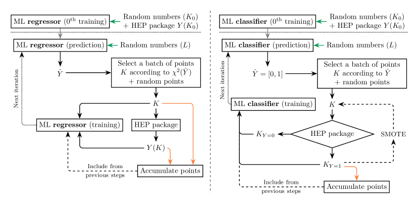
Figure 1: Charts for the ML iterative process used for the regressor (left) and the classifier (right). The main predict-train loop is indicated with black arrows, green arrows indicate places where a random number set is required and the orange arrow marks where we collect the output points. The points accumulated up to step $n_{k}$ are added for training during step $n_{k+1}$.

It is assumed that the calculation of the observables is done through an expensive, time consuming computation, such that it is worthwhile spending additional time training a ML model with its results. Taking these basic steps as the starting point, one can further fill in the details of the sampling, considering that there is a number of ML models to choose from and that the selection of the set $K$ depends highly on the region of interest. Regarding the choice of the set $K$, in general it is a good idea to add an amount of points chosen at random to enforce exploration of new parameter space regardless of the suggestion of the ML model. It is useful to gather the $K$ set and the results from the HEP calculation in every iteration as they represent the sampling of the parameter space. For the training step we always use the new points from the corresponding iteration, but we have the choice to add all or some of the set of accumulated points. After a large amount of points have been accumulated training on the full set may be time consuming, therefore, it would be a good idea to devise rules on how to include them. For example, in Ref. [16] the full set of accumulated points is used to train after a fixed number of iterations. In what follows we will describe our implementation of two broad types of models: ML regressors and ML classifiers.

We will use a ML regressor whenever we are interested in training a model to predict actual outputs from the calculation of observables. In this case the training requires parameter values and their numerical results from the HEP calculation. When we pass a large number of parameter values we get a set of predictions for the observables, $\hat{Y}$, that can aid in the selection of the regions of interest. In this case, the $K$ set could be composed of relevant points based on, e.g., $\chi^{2}$ or likelihood values. However, one could devise any number of selection mechanisms that take advantage of the access to predictions for the observables. The precision of this predictions is expected to be improved with more iterations and this can be easily checked via measures such as the mean absolute error (MAE). After several iterations, using this process should result in a parameter space sampling heavily weighted towards the region of interest used to select the $K$ set and a model specialized in giving accurate and fast predictions for this region.

A different approach would be training a ML classifier to predict if a point in the parameter space would be classified as inside or outside the region of interest according to conditions set by the study being performed. Examples of this conditions would be whether or not the parameter point is theoretically viable and if the point is still inside constraints set by experiments, among several others options. In contrast to the regressor described above, in this case, we expect a binary output from the HEP calculation, say, 1 if the point is inside, 0 if outside. However, after training the ML model, the predictions, $\hat{Y}$, would be distributed in the range $[0,1]$. This presents different opportunities for the selection of points, considering that this prediction can be interpreted as how likely a point is to be classified as inside or outside the desired region. A simple choice would be to take $K$ from the points most likely to be inside. Another choice could be taking points around $\hat{Y}=0.5$, where the model is more uncertain, or even a combination of different ranges. One advantage of already having this classification of points, is that we can try to balance training with sets of equal size for the two classes of points and apply boosting techniques if any class is undersampled. One example of boosting technique is the synthetic minority oversampling technique (SMOTE) [23] that will be explained later in the text. Another advantage of a classification is that it allows the accumulation of a sample of points inside the allowed parameter space in separation from the sample of points outside that needs to be kept to train the model.

On an important note, the danger of overtraining is avoided, in every iteration, by comparing with the true calculation and correcting regions where the ML model is giving wrong advise. For the regressor, since we focused mostly on training inside the region of interest, this means that there is a chance of larger error in predictions outside this region. Obviously, the expectation is that the process outlined above keeps this error under control to avoid missing relevant regions. The case of the classifier is different. Since here we deal with a calculation that decides whether or not a point is in the target region, the trained model responds with how confident it is that a new point belongs inside or outside. Therefore, we require the model to accumulate enough confidence to give certain enough predictions for both classes.

In Fig. 1 we show flowcharts of the iterative process followed for both the ML regressor (left) and the ML classifier (right). Both of them start with an initial $0^{\text{th}}$ training step and proceed to the first prediction step inside the iterative steps. The green arrows indicate the places where sets of random parameters have to be inserted and orange arrows indicate the steps where points are accumulated in the sampled parameter space pool.

3 Application to a multidimensional toy model

In this section we apply the iterative process described in the previous section to a simple model in 3 dimensions. For this model it is possible to find several curved regions of interest that are completely disconnected while also encircling regions of low relevance. While these two features hardly capture all the complexity that can appear when scanning the parameters of a realistic multidimensional model, with this toy model it is shown how, by means of the processes outlined in the last section, these two generic complications are easily addressed.

The 3-dimensional toy model is given by the function

$$O_{\text{3d}}=\left[2+\cos\left(\frac{x_{1}}{7}\right)\cos\left(\frac{x_{2}}{7}\right)\cos\left(\frac{x_{3}}{7}\right)\right]^{5}$$ (1)

where we will use a preferred region with center at $c_{\text{3d}}=100$ and a standard deviation of $\sigma_{\text{3d}}=20$. We will take a gaussian likelihood given by $\mathcal{L}_{\text{3d}}=\exp[-(O_{\text{3d}}-c_{\text{3d}})^{2}/2\sigma_{\text{3d}}^{2}]$ This choice of central values and deviations results in shell-shaped regions of interest for this 3-dimensional model.

To the toy model we will apply sampling with both regression and classification to illustrate the advantages of each approach and demonstrate the differences in the obtained results. We will be using a particular type of DNN, namely, a multi-layer perceptron (MLP), with fully connected layers. The network will be constructed with 4 hidden layers, each of them with 100 neurons, and ReLU activation function. The final layer will have one neuron with a linear activation function in the case of the regressor and a sigmoid activation function for the classifier. For the loss function we will use the mean squared error for the regressor and binary cross entropy for the classifier. In both cases we use the Adam optimizer with a learning rate of 0.001, exponential decay rates $\beta_{1}=0.9$ and $\beta_{2}=0.999$, and train during 1000 epochs. For all the dimensions of the toy model ($j=1,2,3$) we will scan in the range $x_{j}\in[-10\pi,10\pi]$.

To test the ML regressor, we will select the $K$ set using 90% points with a likelihood above 0.9 with the likelihood calculated for the set of predictions $\hat{Y}$ from the ML model. The other 10% will be taken randomly from the parameter space. For training, we will include the accumulated set of points every 2 iterations and in the final iteration to improve the accuracy of the model. When using a regressor, we accumulate all the suggested points which should start to accrue around the region of interest which in our case would be points above the likelihood mentioned before.

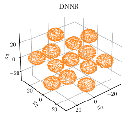
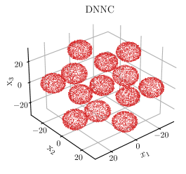
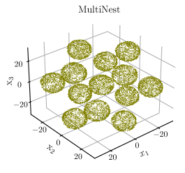
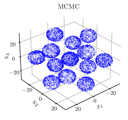
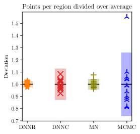
Figure 2: Coverage for 13 different regions of the toy model with 20 000 points, using DNNR (top left), DNNC (top right), MultiNest (middle left) and MCMC (middle right). Best result (less deviation) out of 10 runs is displayed. In the bottom panel we show standard deviations for the 13 regions averaged over 10 runs. The deviation has been normalized to average points per region. Markers show the distribution of the best run out of 10, corresponding to the points in the top 4 panels.

For the ML classifier, the selection of the $K$ set will be composed of 90% chosen depending on the prediction of the classifier and 10% of points chosen at random. The condition for a point to be predicted as inside is that $\hat{Y}>0.75$, points predicted $0.75\leq\hat{Y}\leq 0.25$ are considered uncertain, and points with $\hat{Y}<0.25$ are considered as predicted outside. We aim for a composition where we train with a balanced number of points in each class, therefore, for the 90% non-random part of $K$ we selected 50% from the set predicted inside, and 50% from the uncertain set and points predicted outside. This ratio could be adjusted depending on the accuracy of the model, e.g., increase the fraction of points predicted inside if the accuracy is low. After calculating the actual classification for the suggested points, if the resulting sizes of the groups are imbalanced we can apply a boosting method as will be explained in the next subsection. For training, we always make sure of using an equal amount of points in each true class. In particular, it is important to train on points that have been predicted in the wrong class and points with uncertain predictions, as well as including points from the random set. Since for the classifier we have a clear distinction between classes, at the end we report the amount of points accumulated for the class inside the region of interest.

The results from sampling the parameter space for the toy model using the regressor and classifier is shown in the upper row of Fig. 2. We accumulated a total of roughly 20 000 points with the condition $\mathcal{L}_{\text{3d}}>0.9$. For both DNNR and DNNC we start with an initial set of 500 random points and in every iteration we use the DNN to select 500 points that are passed to the likelihood calculation. It is important to note that the regions of interest are hollow shells of approximately spherical shape. To compare the coverage against other sampling methods, we use PyMultiNest [24] and emcee [25] implementations of MultiNest [3, 4] and MCMC [2], respectively. For emcee we use 500 walkers with other setting left as default. In the case of PyMultiNest we increased the number of active points to 6200 (n_live_points) and reduced the efficiency to 0.5 (sampling_efficiency). The increase of live points is aimed at collecting around 20 000 points with $\mathcal{L}_{\text{3d}}>0.9$. In order to force both emcee and PyMultiNest to concentrate on the region with $\mathcal{L}_{\text{3d}}>0.9$, we apply a weight depending on the value of $\mathcal{L}_{\text{3d}}$ according to

$$\mathcal{W}=\begin{cases}\epsilon&\text{if }\mathcal{L}_{\text{3d}}\leq 0.89\\ 1&\text{if }\mathcal{L}_{\text{3d}}\geq 0.91\\ 50(1-\epsilon)(\mathcal{L}_{\text{3d}}-0.89)+\epsilon&\text{if }0.89<\mathcal{L}_{\text{3d}}<0.91\end{cases}$$ (2)

where the last case is just $\mathcal{W}$ growing linearly to connect the two different $\mathcal{L}_{\text{3d}}$ regimes. For all the examples shown in Fig. 2, we run the sampling method 10 times and display only the points with $\mathcal{L}_{\text{3d}}>0.9$ with the least deviation between disconnected regions. Expectedly, using MCMC results in the least uniformly covered regions with DNNR having the most uniform coverage. Visually, the spread of points using DNNR and DNNC appears more uniform that in the other two examples. In the bottom panel of the same figure we show the average deviation for all the 10 runs in solid light color. The strong colored markers show the deviations in all 13 regions for the run with the least deviation. All the deviations have been normalized to the average points per region in the corresponding run and in all runs we have collected roughly 20 000 points. The DNNR shows the least deviation ($\pm 0.03$) while DNNC sits at $\pm 0.13$. DNNC performs somewhere in between MultiNest ($\pm 0.044$) and MCMC ($\pm 0.26$). The red $\times$ markers for DNNC show that it is possible to have runs with much less deviation than the average.

To comment on the most notable difference between the ML regressor and classifier, the fact that the classifier explicitly distinguishes two classes makes possible to operate differently on the points depending on where they have been classified. Above we mention that we have control over how we pick up points for the training step from the accumulated pools of the two classes. To expand on the classifier, in the next section we show how we can use a small amount of points to actively balance situations where one of the classes tends to be oversampled.

3.1 Boosting the start up convergence

Unlike the ML regressor, in the case of the ML classifier both classes of points are of equal importance. Accordingly, points outside the region of interest are also accumulated to train the model to find their subspace. Therefore, we train the model using data sets of the same size. When the subspace of points of one class is comparably much smaller than that of the other class, the ML model is inefficient to suggest enough points of the smaller class to pass to the HEP calculation in the initial steps, leading to slow convergence. Moreover, we end up training the model with much more points from one class than the other. There are several ways to rectify this imbalance of the data:

• Undersampling the majority class. In this case we loose much of the information from the undersampled class causing the model to converge more slowly.

• Oversampling the minority class by creating random copies from the underrepresented set [16]. This makes the model overestimate the majority class during the test step.

• Oversampling the minority class using SMOTE [23]. The SMOTE transformation is an oversampling technique in which the minority class is enhanced by creating synthetic samples rather than by oversampling with replacement. This technique involves taking each point from the minority class and introducing synthetic samples along the line segments joining them to their nearest neighbors. Depending on the amount of oversampling required, a number $n$ of nearest neighbors can be randomly chosen. After this, a synthetic sample is generated from the lines between a point and its $n$ nearest neighbors depending on the amount of oversampling required.

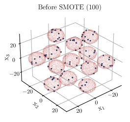
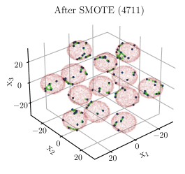
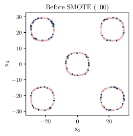
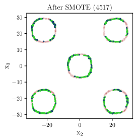
Figure 3: Effect of the SMOTE technique on the toy model of Eq. (1). On the upper panels, an initial set of 100 points (left, dark blue) in the target region is increased to 4743 (right, dark blue and green). In the bottom panels, we apply SMOTE to the $x_{1}=0$ slice of Eq. (1) to increase 100 points in the target region to 4517, where colors have identical meaning to the upper panels. In both upper and bottom panels the SMOTE technique boosts the minority class using 3 nearest neighbors. The proportion of points suggested by SMOTE that are actually in the target region is around 50% for the upper panels and around 90% for the bottom panels. The light red points indicate the target region in all the panels.

The result of oversampling the minority class using SMOTE is shown in Fig. 3 where the minority class (dark blue points) with 100 points is oversampled to around 5000 points according to the description of the process given above.

As mentioned above, we attempt to take a set $K$ made of 90% with predicted $\hat{Y}>0.5$ expecting that the HEP calculation finds most of them with $Y=1$, while the other 10% is taken randomly. If the corrected classes, as given by the HEP calculation, have different sizes we use SMOTE to oversample the minority class. The points suggested by SMOTE are then passed to the HEP calculation for proper classification. It is important to mention that the number of the nearest neighbors used by SMOTE is a hyperparameter that has to be adjusted according to the study under consideration. In Fig. 4 we compare the number of accumulated points after 100 iterations when SMOTE is applied (orange) and not applied (blue) to oversample the minority class ($Y=1$ in this case) and in case of undersampling the majority class. We found that for the 3-dimensional toy model, Eq. (1), with $K_{0}=10\,000$, $L=3000$ and $K=200$ the model is able to accumulate 5 times more points when SMOTE is employed.

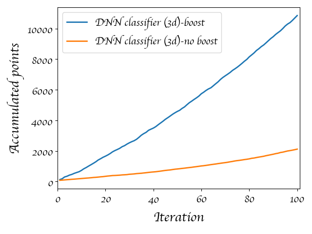
Figure 4: Number of accumulated points in terms of iterations when using (blue) and not using (orange) the boosting method, for the 3-dimensional toy model. The sizes of the sets $K_{0}$, $L$ and $K$ as well as details for the selection of points are described in the text.

4 Learning the Higgs signal strength in type II 2HDM

In this section we show the performance of ML models scanning over the parameter space of the type II 2HDM scalar potential to match the measured Higgs signal strength.

4.1 The model

The 2HDMs [26, 27] are extensions of the SM scalar sector containing two $SU(2)_{L}$ doublets, $\phi_{1}$ and $\phi_{2}$, sharing identical charge assignments under the SM gauge symmetry group:

$$\phi_{1}=\begin{pmatrix}\eta_{1}^{+}\\ (v_{1}+h_{1}+ih_{3})/\sqrt{2}\\ \end{pmatrix},\qquad\phi_{2}=\begin{pmatrix}\eta_{2}^{+}\\ (v_{2}+h_{2}+ih_{4})/\sqrt{2}\\ \end{pmatrix}\,.$$ (3)

The 4 real fields are labeled $h_{i}$, with $i=1,\ldots,4$; the complex charged fields are $\eta_{i}^{+}$, with $i=1,2$; the vacuum expectations values (VEVs) are $v_{i}$, with $i=1,2$.

The scalar setup in the 2HDM allows for flavor changing neutral currents (FCNC) from the Yukawa terms, which are restricted by current measurements. A 2HDM with no FCNC can be obtained by adding a softly broken global $Z_{2}$ symmetry [28] where $(\phi_{1},\phi_{2})\to(\phi_{1},-\phi_{2})$. In this case, the most general scalar potential is given by

$$\begin{split}V_{\phi}=&m^{2}_{11}(\phi^{\dagger}_{1}\phi_{1})+m^{2}_{22}(\phi^{\dagger}_{2}\phi_{2})-\left[m^{2}_{12}(\phi^{\dagger}_{1}\phi_{2})+\text{h.c.}\right]+\lambda_{1}(\phi^{\dagger}_{1}\phi_{1})^{2}+\lambda_{2}(\phi^{\dagger}_{2}\phi_{2})^{2}\\ &+\lambda_{3}(\phi^{\dagger}_{1}\phi_{1})(\phi^{\dagger}_{2}\phi_{2})+\lambda_{4}(\phi^{\dagger}_{1}\phi_{2})(\phi^{\dagger}_{2}\phi_{1})+\frac{1}{2}\left[\lambda_{5}(\phi^{\dagger}_{1}\phi_{2})^{2}+\text{H.c.}\right]\,,\end{split}$$ (4)

where $m_{12}^{2}$ softly breaks the $Z_{2}$ symmetry. In $V_{\phi}$, the parameters $m_{jj}^{2}$ and $\lambda_{i\neq 5}$ are real, while $m^{2}_{12}=|m^{2}_{12}|e^{i\eta(m^{2}_{12})}$ and $\lambda_{5}=|\lambda_{5}|e^{i\eta(\lambda_{5})}$ are complex parameters that allow for CP violation [34, 35]. In the following we consider a real potential with vanishing complex phases, $\eta(\lambda_{5})=\eta(m^{2}_{12})=0$. The VEVs $v_{1}$ and $v_{2}$ are related to the SM VEV by $v=\sqrt{v_{1}^{2}+v_{2}^{2}}\sim 246$ GeV, and their ratio is defined as $\tan\beta\equiv v_{2}/v_{1}$.

The mass terms, $m^{2}_{11}$ and $m^{2}_{22}$, are determined from the minimization conditions of the scalar potential. Four physical scalars are obtained after diagonalizing the mass matrices, with two CP even Higgses ($h_{1},h_{2}$), one CP odd scalar ($A$) and one charged Higgs ($H^{\pm}$) with masses given by

$$m^{2}_{h_{1,2}} =\frac{1}{2}\left[\chi^{2}_{11}+\chi^{2}_{22}\mp\sqrt{(\chi^{2}_{11}-\chi^{2}_{22})^{2}+4(\chi^{2}_{12})^{2}}\right]\,,$$ (5)

$$m^{2}_{A} =\frac{2m^{2}_{12}}{\sin 2\beta}-\lambda_{5}v^{2}\,,$$ (6)

$$m^{2}_{H^{\pm}} =\frac{2m^{2}_{12}}{\sin 2\beta}-\frac{1}{2}(\lambda_{4}+\lambda_{5})v^{2}\,,$$ (7)

with

$$\chi^{2}_{11} =m^{2}_{12}\tan\beta+2\lambda_{1}v^{2}\cos^{2}\beta\,,$$ (8)

$$\chi^{2}_{22} =m^{2}_{12}\cot\beta+2\lambda_{2}v^{2}\sin^{2}\beta\,,$$ (9)

$$\chi^{2}_{12} =-m^{2}_{12}+\frac{1}{2}(\lambda_{3}+\lambda_{4}+\lambda_{5})v^{2}\sin 2\beta\,.$$ (10)

For the type-II 2HDM, the Yukawa terms that respect the $Z_{2}$ symmetry are written in the form

$$-\mathcal{L}_{Y}=Y_{u}\overline{Q}_{L}\tilde{\phi}_{2}u_{R}+Y_{d}\overline{Q}_{L}\phi_{1}d_{R}+Y_{\ell}\overline{L}_{L}\phi_{2}\ell_{R}+H.c\,,$$ (11)

where $\tilde{\phi}_{2}=i\tau_{2}\phi_{2}^{*}$, $\tau_{2}$ is the $SU(2)$ generator corresponding to the Pauli matrix $\sigma_{2}$ and $Y_{u},Y_{d},Y_{\ell}$ are $3\times 3$ Yukawa coupling matrices.

We perform a scan over seven free parameters of the potential, $\lambda_{j}$ ($j\in\{1,2,3,4,5\}$), $\tan\beta$ and soft $Z_{2}$-breaking mass $m^{2}_{12}$, to adjust the SM-like Higgs properties to match current measurements, taking into account other constraints from the electroweak global fit and B meson decays. Note that one has the freedom to scan over physical parameters instead. Each parameter base has their own advantages, for example, using parameters of the potential allows to choose ranges where stability and perturbativity test are automatically passed. We use SPheno-4.0.5 [29] to calculate the particle spectrum of the physical eigenstates, FlavorKit [38] for B meson decays while HiggsBounds-5.3.2 [30, 31] and HiggsSignals-2.2.3 [32, 33] are used to constraint the parameter space using recent Higgs boson measurements. HiggsBounds constrains the parameter space by computing the theoretical prediction for the most sensitive channel for each scalar, $h_{i}$, and dividing by the observed experimental value to obtain the ratio, $\mathcal{O}_{i}$. The computation of $\mathcal{O}_{i}$ requires production cross sections, $\sigma$, and decay branching ratios, $\mathrm{BR}(h_{i})$, as in

$$\mathcal{O}_{i}=\frac{[\sigma\times\mathrm{BR}(h_{i})]_{\text{model}}}{[\sigma\times\mathrm{BR}(h_{i})]_{\text{obs}}}\,,$$ (12)

where a value $\mathcal{O}_{i}>1$ corresponds to a parameter point excluded by the $95\%$ C.L. limit. HiggsSignals constrains the parameter space by evaluating the statistical compatibility of the SM-like Higgs boson in the model using recent data for the $125$ GeV Higgs resonance observed at the LHC. HiggsSignals reports a total $\chi^{2}$ value for testing the model hypothesis as a combination of $\chi^{2}_{\mu}$ from the signal strength modifiers and $\chi^{2}_{m_{h_{i}}}$ from corresponding predicted Higgs masses as

$$\chi^{2}_{\text{tot}}=\chi^{2}_{\mu}+\sum^{N_{h}}_{i=1}\chi^{2}_{m_{h_{i}}}.$$ (13)

The best fit value is calculated according to

$$\chi^{2}_{\text{best}}=\chi^{2}_{\text{min}}/n_{\text{D.O.F.}}\,.$$ (14)

with $\chi^{2}_{\text{min}}$ the minimum $\chi^{2}$. We adjust our selection to accept all points with $\chi_{\text{tot}}^{2}\leq 95$, with a SM Higgs mass uncertainty of $\pm 2$ GeV. It is worth mentioning that all selected points are required to pass the HiggsBounds selection.

4.2 Additional constraints

The oblique parameters from the electroweak observables fit receive contributions from the 2HDM at one-loop level, constraining the 2HDM parameter space. From the global fit of the oblique parameters we have [37]:

$$S=0.03\pm 0.10\,,\hskip 11.38109ptT=0.05\pm 0.12\,,\hskip 11.38109ptU=0.03\pm 0.10\,.$$ (15)

Additionally, measurements from B meson decays add extra constraints on $(m_{H^{\pm}}\text{-}\tan\beta)$ plane. For large $\tan\beta$, the dominant constraints come from $\mathrm{BR}(B^{+}\to\tau^{+}\nu)=(1.06\pm 0.19)\times 10^{-4}$ and $\mathrm{BR}(B\to S\gamma)_{E_{\gamma}\geq 1.6\text{GeV}}=(3.32\pm 0.15)\times 10^{-4}$[36]. The ranges for mentioned branching ratios are displayed in the left side of Fig. 5.

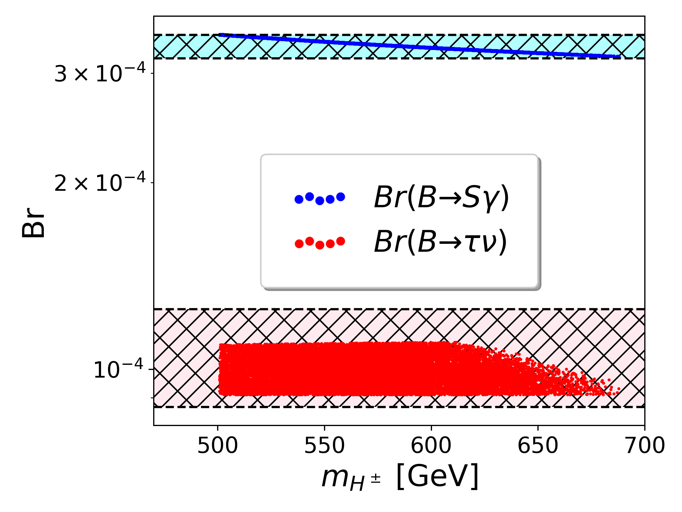
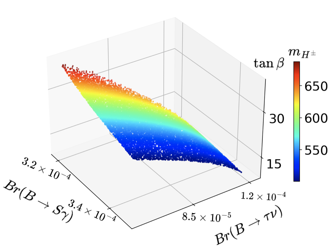
Figure 5: Accumulated points from MLP classifier model. Left: branching ratios of $B\to S\gamma$ (blue points) and $B\to\tau\nu$ (red points) versus the charged Higgs mass, while the shaded cyan and pink areas are the current allowed regions from $B\to S\gamma$ and $B\to\tau\nu$ respectively at re-fitted $1\sigma$ reported in [36]. Right: Relationship between both branching ratios displayed on the left and $\tan\beta$, colored according to the value of the charged Higgs mass.

4.3 Numerical scan details

Since the ML classifier is only concerned with points passing the conditions mentioned above, it is less affected by a fast changing total $\chi^{2}$ than the regressor

Therefore, we can consider wider ranges without a dramatic increase in the required initial number of points. Considering this, we scan over the following ranges

$$\begin{gathered}0\leq\lambda_{1}\leq 10,\qquad 0\leq\lambda_{2}\leq 0.2,\qquad-10\leq\lambda_{3}\leq 10,\qquad-10\leq\lambda_{4}\leq 10,\\ -10\leq\lambda_{5}\leq 10,\qquad 5\leq\tan\beta\leq 45,\qquad-3000\text{ GeV}^{2}\leq m^{2}_{12}\leq 0\text{ GeV}^{2}\,,\end{gathered}$$ (16)

where positive $\lambda_{1}$ and $\lambda_{2}$ are required for vacuum stability. In order to keep the light Higgs, $h_{1}$, as the SM-like Higgs of the model we consider a rather narrow range for $\lambda_{2}$ and use negative values for the soft $Z_{2}$-breaking mass parameter $m^{2}_{12}$.

We use a sequential MLP with four hidden layers with 100 neurons in each layer and ReLU activation function. The output layer has one neuron with Sigmoid activation which maps the output to probabilities between 0 and 1. We train during 1000 epochs. The loss function, binary cross entropy, is minimized by Adam optimizer with learning rate of 0.001 and exponential decay rates $\beta_{1}=0.9$ and $\beta_{2}=0.999$. In each iteration we select $K$ points from the ML predictions. The sampled $K$ points are then passed to the HEP packages to classify them. In the steps where the data sets are imbalanced, SMOTE is automatically called to oversample the minority class. Additionally, the training data are normalized according to the standard normal distribution.

For the ML regressor, We use a sequential MLP with four hidden layers each with 100 neurons and ReLU activation function. The final output layer contains only one neuron with linear activation function. The loss function in this case is the mean squared error which is minimized by Adam optimizer with learning rate of 0.001 and exponential decay rates $\beta_{1}=0.9$ and $\beta_{2}=0.999$. We train during 1000 epochs in every step. The collected samples are fully utilized to train the ML model after every two iterations, without validation and test samples, since calculating observables precisely using HEP packages is time consuming.

As for the toy model, here we compare against sampling using MCMC and MultiNest. Considering that in this case we do not have several identically shaped regions as in the case of the toy model, we compare against the efficiency in every iteration, defined as the number of in-target points over the number of tried points. For the MCMC we use emcee, we start with 300 in-target points with walkers 300 walkers using as log(likelihood) function the HiggsSignals $\chi^{2}$ plus all the other constraints discussed above. For Multinest we use PyMultiNest with log-likelihood function as the MCMC.

In Fig. 6 we show the efficiency for the 4 different methods, ML classifier (DNNC), regressor (DNNR), MCMC and MultiNest as the number of collected points per iteration over batch size (300). For all methods we require to collect 20 000 points.

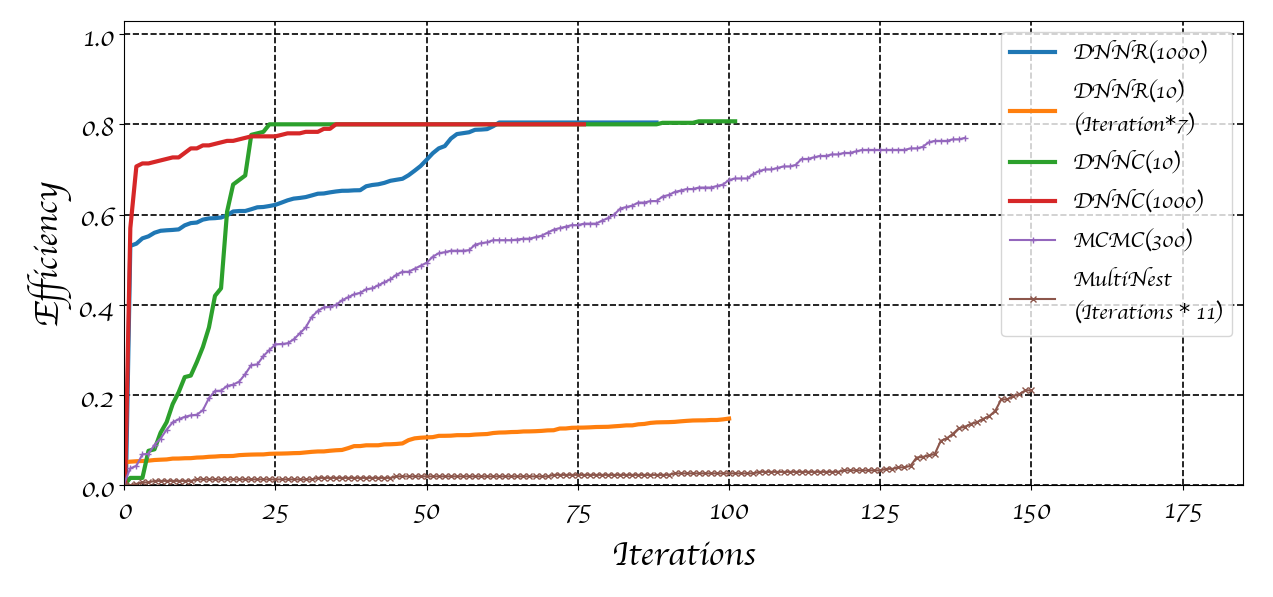
Figure 6: Efficiency in every iteration for different methods. For all the methods we run enough iterations to accumulate 20 000 points. The number in parenthesis indicates the initial in-target points for each method, except MultiNest. For some methods we have scaled the iterations by a factor indicated as “Iteration*$x$”, meaning actual iterations is number in $x$-axis times this number.

Considering that the convergence efficiency for the DNNC and DNNR depends on the initial number of in-target points, we compare the efficiency with different sizes for initial in-target points, 10 and 1000 points. For both, DNNC and DNNR, we sample the batch $K=300$ from $L=200\,000$ with $20\%$ random points. For DNNR with 1000 initial in-target points (blue line) we accumulate 20 000 points after 88 iterations while for DNNC with the same initial in-target points (red line) it requires 77 iterations. Here we point out that the maximum efficiency is $\sim 80\%$ since $20\%$ points are chosen randomly in each iteration. DNNR with 10 initial in-target points (orange line) has a far slower convergence requiring 700 iterations to accumulate 20 000 points in-target. In the case of the DNNC with 10 initial in-target points (green line), the SMOTE technique suggests enough new synthetic points in the target region, resulting in an increase of efficiency. For this case, efficiency is calculated after correcting with SMOTE (see Fig. 1). This case requires 100 iterations to accumulate the 20 000 points. For MCMC accumulating 20 000 points requires 140 iterations, adding each time more in target points, although, at a lower rate than DNNR(1000), DNNC(10) and DNNC(1000). And MultiNest expectedly spends several iterations in the beginning exploring the regions with lower likelihood, requiring a total of 1560 iterations.

4.4 MLP classifier results

As already discussed, MCMC and MultiNest require the evaluation of the log-likelihood from the HEP package for all the tested points, which may lead to longer computation time when acceptance is low. Moreover, convergence for the DNNR depends heavily on having a big enough set of in-target points. This means that for large sampling space and small target region the regressor model tends to take longer to start converging. In the case of the DNNC, we handle this problem with SMOTE as technique to collect more in-target points in the first steps and accelerate the initial convergence. As the DNNC method shows better performance on efficiency as iterations accumulate, we show the allowed ranges for the 2HDM-II scalar potential parameters and physical observables from our DNNC scan.

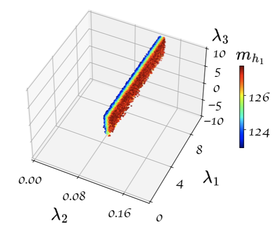
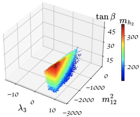
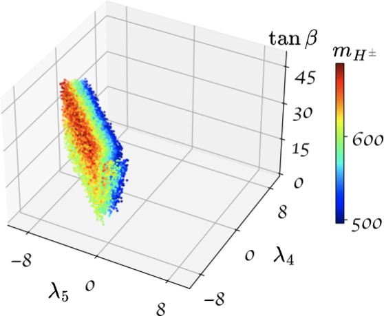
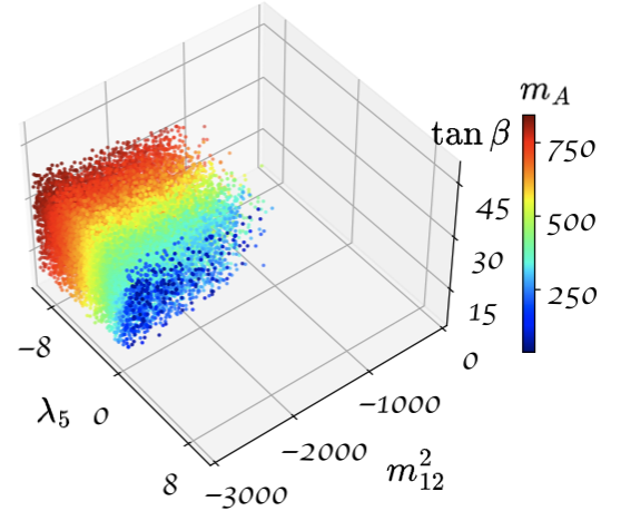
Figure 7: Allowed scalar potential parameters with 20 000 points. Color represents the mass of physical scalars according to the corresponding colorbar. All masses are given in GeV ($m^{2}_{12}$ in GeV²).

Accumulated points satisfy all theoretical and experimental constraints mentioned in Secs. 4.1 and 4.2. The obtained allowed ranges are the following

$$\begin{gathered}1.3\times 10^{-3}\leq\lambda^{\text{allowed}}_{1}\leq 10,\quad 0.12\leq\lambda^{\text{allowed}}_{2}\leq 0.14,\quad 4.1\leq\lambda^{\text{allowed}}_{3}\leq 9,\\ -10\leq\lambda^{\text{allowed}}_{4}\leq 5.3,\quad-10\leq\lambda^{\text{allowed}}_{5}\leq 1.55,\quad 10\leq\tan\beta^{\text{allowed}}\leq 38,\\ -3000\text{ GeV}^{2}\leq(m^{2}_{12})^{\text{allowed}}\leq-768\text{ GeV}^{2}\,.\end{gathered}$$ (17)

Considering these ranges for the scalar potential parameters, in Fig. 7 we show 3-dimensional projections for several parameters with color for the masses of different physical scalars. The SM-like Higgs, $h_{1}$, the lightest scalar in our setup, shows a large dependence on $\lambda_{2}$, that results in a narrowly distributed region in the upper left panel of Fig. 7. This sharp dependence in $\lambda_{2}$ can be explained with Eq. (9) where, for large $\tan\beta$, the largest contributions comes from $2\lambda_{2}v^{2}\sin^{2}\beta$. Considering that large $\tan\beta$ implies $\sin\beta\sim 1$ and $v^{2}$ is fixed, from Eq. (5) we can deduce that $m_{h_{1}}$ depends heavily on the value of $\lambda_{2}$. Conversely, the mass of the heavier Higgs, $h_{2}$, depends on $m^{2}_{12}$ and $\tan\beta$ through $\chi^{2}_{11}$ in Eq. (5), as shown in the upper right panel of Fig. 7. For the charged Higgs, $H^{\pm}$, the mass depends on a combination of $m^{2}_{12}$, $\lambda_{4}$, $\lambda_{5}$ and $\beta$. In the lower left panel of Fig. 7 can be seen clearly that $m_{H^{\pm}}$ depends on the combination of $\lambda_{4}$ and $\lambda_{5}$. It is also possible to see that larger values of $m_{H^{\pm}}$ are obtained for larger $\tan\beta$. In the case of the mass of the pseudoscalar, $A$, it depends on a combination of $\lambda_{5}$, $m^{2}_{12}$ and $\beta$. Considering the scan range for $m^{2}_{12}$, the pseudoscalar mass is strongly sensitive to $\lambda_{5}$ as shown the lower right panel of Fig. 7.

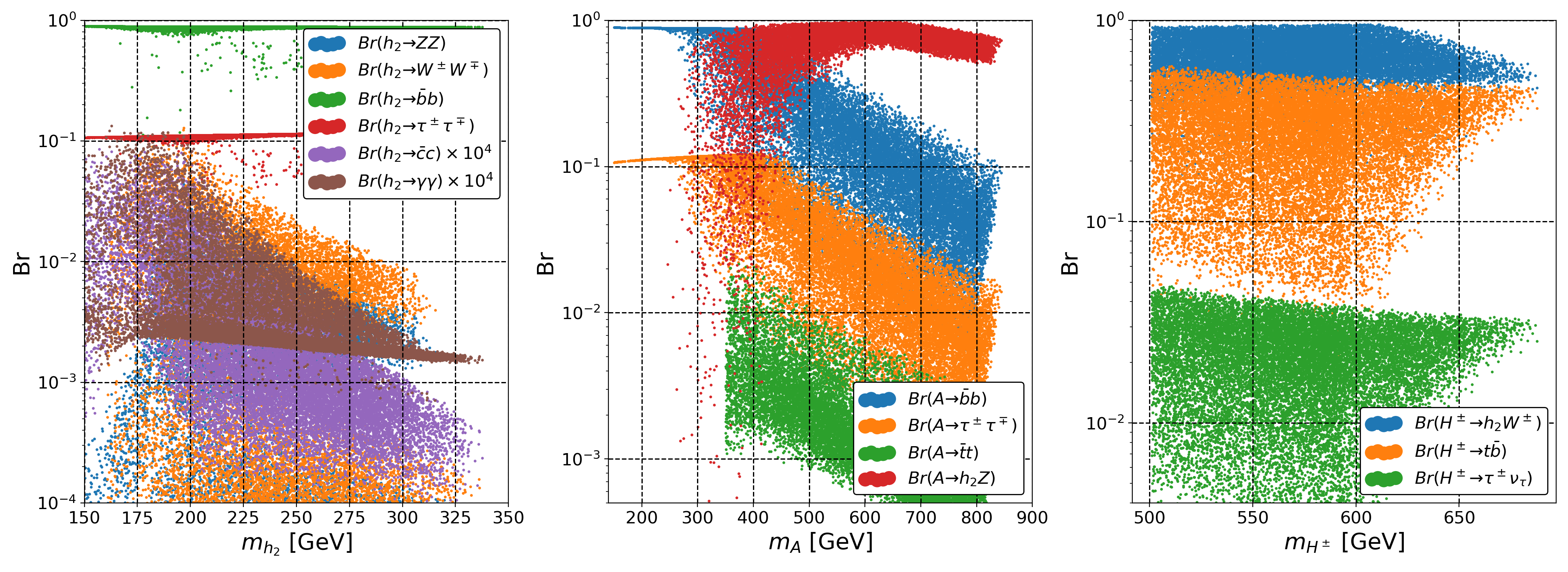
Figure 8: Dependence of branching ratios on the masses of the BSM scalars, $h_{2}$ (left), $A$ (middle) and $H^{\pm}$ (right), using the accumulated 20 000 points. Branching ratios for the SM-like Higgs, $h_{1}$, are fixed by HiggsSignals to experimental measurements.

Branching ratios for $h_{2}$, $A$ and $H^{\pm}$ scalar bosons are shown in Fig. 8. In the case of the SM-like Higgs, $h_{1}$, branching ratios have been fixed to experimental measurements by HiggsSignals. The dominant decay of $h_{2}$ is via $b$ quark pair and $\tau$ lepton pair, both proportional to $\cos\alpha/\cos\beta$. Here, $\alpha$ comes from the combination $\alpha-\beta$, which is the angle that diagonalizes the CP-even Higgses squared mass matrix. The di-gauge boson decay of $h_{2}$ is suppressed by $\cos(\alpha-\beta)$ and hence subdominant, as shown in the left pane of Fig. 8. This supression is expected, since it is a consequence of experimental constraints that force the 2HDM-II closer to the decoupling limit, $\cos(\alpha-\beta)\sim 0$. In the middle panel of Fig. 8, we show the branching ratios of the pseudoscalar, $A$, which, for $m_{A}\lesssim 300$ GeV, is dominated by $b$ quark pair and $\tau$ lepton pair. This is expected since $A$ decaying to pair of down-type quark pair or lepton pair is proportional to $\tan\beta$ which we assume to be large. In the case of decays into pairs of up-type quarks, like $t$, we have suppression by $\cot\beta$. The dominant decay mode for $m_{A}\gtrsim 400$ GeV is Br$(A\to h_{2}Z)$, whenever $m_{A}>m_{h_{2}}+m_{Z}$, which is proportional to $\sin(\alpha-\beta)$. For the charged Higgs, decay is dominated by Br$(H^{\pm}\to h_{2}W^{\pm})$ which is proportional to $\sin(\alpha-\beta)$, while the fermionic decays are suppressed by $\cot\beta$, as can be seen in the right side of Fig. 8.

5 Conclusion

In this paper we have discussed the implementation of two broad types of ML based approaches for efficient sampling of multidimensional parameter spaces: regression and classification. The ML model is employed as part of an iterative process where it is used to suggest new points and trained according to the results of this suggestion. In the case of the regression we train a ML model to precisely predict observables in regions favoured by observations. For the classification we train the model to be able to separate the points that belong to the region of interest from those outside of it. In the case of the classification we devise a process to alleviate undersampling of small regions employing SMOTE. We find that both approaches can efficiently sample regions of interest with features like several disconnected regions or regions of low interest inside regions of high interest. In particular, we applied the two types of model to a 3-dimensional toy model using sphere-like shell regions as target space. We compared sampling in this toy model against results from other methods used to determine relevant regions in parameter space, namely MCMC (as implemented in emcee) and MultiNest. We found that, for both regressor and classifier, it is possible to achieve a uniform sampling of all regions of interest with comparable or better distribution. Moreover, for the classification model we found that using the SMOTE technique to balance the sampling of the classes can considerably improve the accumulation of points when compared to not applying any balancing method. To illustrate results for a HEP model, we sampled the parameter space of the 2HDM by integrating our iterative implementation with popular HEP packages that take care of calculating the theoretical and experimental results. We found that we can accumulate points on regions of interest, defined by $\chi^{2}$ ranges, even when some parameters are narrowly distributed inside the scanned region. In particular, the classifier using the SMOTE technique to accelerate convergence of the model in the first few iterations can rapidly approach maximum efficiency. We compare against the efficiency obtained when sampling with MCMC and MultiNest. Expectedly, efficiency for our classifier is much higher since it is designed to concentrate on the target region. However, the use of neural networks and iterative training allow uniform sampling of parameters regardless of whether their distribution is wide or narrow. We finalize showing results for the sampled parameter space, including masses of the physical scalars and their obtained branching fractions. Note that there is plenty of space for extensibility, beyond the characteristics of the employed neural networks. For example, different types of problems may benefit from more sophisticated choices of points for training, using information like disagreement between the trained model and the full calculation. This possibilities are left for future improvement of the techniques described in this work. The code used for the examples presented here and corresponding documentation is freely available on the web.

References

- [1] R. L. Workman [Particle Data Group], “Review of Particle Physics,” PTEP 2022, 083C01 (2022) doi:10.1093/ptep/ptaa104.
- [2] D.J.C. MacKay, “Information Theory, Inference and Learning Algorithms,” Cambridge University Press, 2003.
- [3] F. Feroz and M. P. Hobson, “Multimodal nested sampling: an efficient and robust alternative to MCMC methods for astronomical data analysis,” Mon. Not. Roy. Astron. Soc. 384, 449 (2008) doi:10.1111/j.1365-2966.2007.12353.x [arXiv:0704.3704 [astro-ph]].
- [4] F. Feroz, M. P. Hobson and M. Bridges, “MultiNest: an efficient and robust Bayesian inference tool for cosmology and particle physics,” Mon. Not. Roy. Astron. Soc. 398, 1601-1614 (2009) doi:10.1111/j.1365-2966.2009.14548.x [arXiv:0809.3437 [astro-ph]].
- [5] A. Lewis and S. Bridle, “Cosmological parameters from CMB and other data: A Monte Carlo approach,” Phys. Rev. D 66, 103511 (2002) doi:10.1103/PhysRevD.66.103511 [arXiv:astro-ph/0205436 [astro-ph]].
- [6] R. Lafaye, T. Plehn and D. Zerwas, “SFITTER: SUSY parameter analysis at LHC and LC,” [arXiv:hep-ph/0404282 [hep-ph]].
- [7] P. Bechtle, K. Desch and P. Wienemann, “Fittino, a program for determining MSSM parameters from collider observables using an iterative method,” Comput. Phys. Commun. 174, 47-70 (2006) doi:10.1016/j.cpc.2005.09.002 [arXiv:hep-ph/0412012 [hep-ph]].
- [8] R. Ruiz de Austri, R. Trotta and L. Roszkowski, “A Markov chain Monte Carlo analysis of the CMSSM,” JHEP 05, 002 (2006) doi:10.1088/1126-6708/2006/05/002 [arXiv:hep-ph/0602028 [hep-ph]].
- [9] B. C. Allanach and C. G. Lester, “Sampling using a ‘bank’ of clues,” Comput. Phys. Commun. 179, 256-266 (2008) doi:10.1016/j.cpc.2008.02.020 [arXiv:0705.0486 [hep-ph]].
- [10] C. Strege, G. Bertone, G. J. Besjes, S. Caron, R. Ruiz de Austri, A. Strubig and R. Trotta, “Profile likelihood maps of a 15-dimensional MSSM,” JHEP 09, 081 (2014) doi:10.1007/JHEP09(2014)081 [arXiv:1405.0622 [hep-ph]].
- [11] C. Han, K. i. Hikasa, L. Wu, J. M. Yang and Y. Zhang, “Status of CMSSM in light of current LHC Run-2 and LUX data,” Phys. Lett. B 769, 470-476 (2017) doi:10.1016/j.physletb.2017.04.026 [arXiv:1612.02296 [hep-ph]].
- [12] P. Athron et al. [GAMBIT], “GAMBIT: The Global and Modular Beyond-the-Standard-Model Inference Tool,” Eur. Phys. J. C 77, no.11, 784 (2017) doi:10.1140/epjc/s10052-017-5321-8 [arXiv:1705.07908 [hep-ph]].
- [13] E. Bagnaschi, K. Sakurai, M. Borsato, O. Buchmueller, M. Citron, J. C. Costa, A. De Roeck, M. J. Dolan, J. R. Ellis and H. Flächer, et al. “Likelihood Analysis of the pMSSM11 in Light of LHC 13-TeV Data,” Eur. Phys. J. C 78, no.3, 256 (2018) doi:10.1140/epjc/s10052-018-5697-0 [arXiv:1710.11091 [hep-ph]].
- [14] T. Brinckmann and J. Lesgourgues, “MontePython 3: boosted MCMC sampler and other features,” Phys. Dark Univ. 24, 100260 (2019) doi:10.1016/j.dark.2018.100260 [arXiv:1804.07261 [astro-ph.CO]].
- [15] J. Ren, L. Wu, J. M. Yang and J. Zhao, “Exploring supersymmetry with machine learning,” Nucl. Phys. B 943, 114613 (2019) doi:10.1016/j.nuclphysb.2019.114613 [arXiv:1708.06615 [hep-ph]].
- [16] M. D. Goodsell and A. Joury, “Active learning BSM parameter spaces,” [arXiv:2204.13950 [hep-ph]].
- [17] M. Feickert and B. Nachman, “A Living Review of Machine Learning for Particle Physics,” [arXiv:2102.02770 [hep-ph]].
- [18] P. Graff, F. Feroz, M. P. Hobson and A. Lasenby, “BAMBI: blind accelerated multimodal Bayesian inference,” MNRAS, 421, 169 (2012) doi:10.1111/j.1365-2966.2011.20288.x [arXiv:1110.2997 [astro-ph]].
- [19] F. Staub, “xBIT: an easy to use scanning tool with machine learning abilities,” [arXiv:1906.03277 [hep-ph]].
- [20] S. Caron, T. Heskes, S. Otten and B. Stienen, “Constraining the Parameters of High-Dimensional Models with Active Learning,” Eur. Phys. J. C 79, no.11, 944 (2019) doi:10.1140/epjc/s10052-019-7437-5 [arXiv:1905.08628 [cs.LG]].
- [21] J. Rocamonde, L. Corpe, G. Zilgalvis, M. Avramidou and J. Butterworth, “Picking the low-hanging fruit: testing new physics at scale with active learning,” SciPost Phys. 13, 002 (2022) doi:10.21468/SciPostPhys.13.1.002 [arXiv:2202.05882 [hep-ph]].
- [22] F. A. de Souza, M. Crispim Romão, N. F. Castro, M. Nikjoo and W. Porod, “Exploring Parameter Spaces with Artificial Intelligence and Machine Learning Black-Box Optimisation Algorithms,” [arXiv:2206.09223 [hep-ph]].
- [23] N. V. Chawla, K. W. Bowyer, L. O. Hall and W. P. Kegelmeyer, “SMOTE: Synthetic Minority Over-sampling Technique,” Journal of Artificial Intelligence Research 16 (2002) 321–357 doi:10.1613/jair.953 [arXiv:1106.1813 [hep-ph]].
- [24] J. Buchner, A. Georgakakis, K. Nandra, L. Hsu, C. Rangel, M. Brightman, A. Merloni, M. Salvato, J. Donley and D. Kocevski, “X-ray spectral modelling of the AGN obscuring region in the CDFS: Bayesian model selection and catalogue,” Astron. Astrophys. 564, A125 (2014) doi:10.1051/0004-6361/201322971 [arXiv:1402.0004 [astro-ph.HE]].
- [25] D. Foreman-Mackey, D. W. Hogg, D. Lang and J. Goodman “emcee: The MCMC Hammer,” Publi. Astron. Soc. Pac. 125, 306–312 (2013) doi:10.1086/670067 [arXiv:1202.3665 [astro-ph.IM]].
- [26] T. D. Lee, “A Theory of Spontaneous T Violation,” Phys. Rev. D 8, 1226-1239 (1973) doi:10.1103/PhysRevD.8.1226
- [27] G. C. Branco, P. M. Ferreira, L. Lavoura, M. N. Rebelo, M. Sher and J. P. Silva, “Theory and phenomenology of two-Higgs-doublet models,” Phys. Rept. 516, 1-102 (2012) doi:10.1016/j.physrep.2012.02.002 [arXiv:1106.0034 [hep-ph]].
- [28] S. L. Glashow and S. Weinberg, “Natural Conservation Laws for Neutral Currents,” Phys. Rev. D 15, 1958 (1977) doi:10.1103/PhysRevD.15.1958
- [29] W. Porod and F. Staub, “SPheno 3.1: Extensions including flavour, CP-phases and models beyond the MSSM,” Comput. Phys. Commun. 183 (2012), 2458-2469 doi:10.1016/j.cpc.2012.05.021 [arXiv:1104.1573 [hep-ph]].
- [30] P. Bechtle, O. Brein, S. Heinemeyer, G. Weiglein and K. E. Williams, “HiggsBounds: Confronting Arbitrary Higgs Sectors with Exclusion Bounds from LEP and the Tevatron,” Comput. Phys. Commun. 181 (2010), 138-167 doi:10.1016/j.cpc.2009.09.003 [arXiv:0811.4169 [hep-ph]].
- [31] P. Bechtle, O. Brein, S. Heinemeyer, G. Weiglein and K. E. Williams, “HiggsBounds 2.0.0: Confronting Neutral and Charged Higgs Sector Predictions with Exclusion Bounds from LEP and the Tevatron,” Comput. Phys. Commun. 182 (2011), 2605-2631 doi:10.1016/j.cpc.2011.07.015 [arXiv:1102.1898 [hep-ph]].
- [32] P. Bechtle, S. Heinemeyer, O. Stål, T. Stefaniak and G. Weiglein, “: Confronting arbitrary Higgs sectors with measurements at the Tevatron and the LHC,” Eur. Phys. J. C 74 (2014) no.2, 2711 doi:10.1140/epjc/s10052-013-2711-4 [arXiv:1305.1933 [hep-ph]].
- [33] O. Stål and T. Stefaniak, “Constraining extended Higgs sectors with HiggsSignals,” PoS EPS-HEP2013 (2013), 314 doi:10.22323/1.180.0314 [arXiv:1310.4039 [hep-ph]].
- [34] S. Antusch, O. Fischer, A. Hammad and C. Scherb, “Testing CP Properties of Extra Higgs States at the HL-LHC,” JHEP 03 (2021), 200 doi:10.1007/JHEP03(2021)200 [arXiv:2011.10388 [hep-ph]].
- [35] S. Antusch, O. Fischer, A. Hammad and C. Scherb, “Explaining excesses in four-leptons at the LHC with a double peak from a CP violating Two Higgs Doublet Model,” JHEP 08, 224 (2022) doi:10.1007/JHEP08(2022)224 [arXiv:2112.00921 [hep-ph]].
- [36] Y. S. Amhis et al. [HFLAV], Eur. Phys. J. C 81 (2021) no.3, 226 doi:10.1140/epjc/s10052-020-8156-7 [arXiv:1909.12524 [hep-ex]].
- [37] M. Baak, M. Goebel, J. Haller, A. Hoecker, D. Kennedy, R. Kogler, K. Moenig, M. Schott and J. Stelzer, Eur. Phys. J. C 72 (2012), 2205 doi:10.1140/epjc/s10052-012-2205-9 [arXiv:1209.2716 [hep-ph]].
- [38] W. Porod, F. Staub and A. Vicente, Eur. Phys. J. C 74 (2014) no.8, 2992 doi:10.1140/epjc/s10052-014-2992-2 [arXiv:1405.1434 [hep-ph]].