The Atlas Benchmark: an Automated Evaluation Framework
for Human Motion Prediction
Abstract
Human motion trajectory prediction, an essential task for autonomous systems in many domains, has been on the rise in recent years. With a multitude of new methods proposed by different communities, the lack of standardized benchmarks and objective comparisons is increasingly becoming a major limitation to assess progress and guide further research. Existing benchmarks are limited in their scope and flexibility to conduct relevant experiments and to account for contextual cues of agents and environments. In this paper we present Atlas, a benchmark to systematically evaluate human motion trajectory prediction algorithms in a unified framework. Atlas offers data preprocessing functions, hyperparameter optimization, comes with popular datasets and has the flexibility to setup and conduct underexplored yet relevant experiments to analyze a method’s accuracy and robustness. In an example application of Atlas, we compare five popular model- and learning-based predictors and find that, when properly applied, early physics-based approaches are still remarkably competitive. Such results confirm the necessity of benchmarks like Atlas.
I Introduction
Benchmarking motion prediction algorithms is a challenging task. The evaluation outcome can be affected by various factors such as data, parameters, hyperparameters and experiment design. Elaborate and carefully designed experiments are necessary to expose specific abilities or limitations of a method, in particular for complex learning approaches. Influencing factors are, for example, the observation period, i.e. the duration that agents need to be seen to allow for accurate prediction of their motion, or the exact procedure how to set up a testing scenario from sequences of raw person detections. Even when evaluating a simple constant velocity motion model with the same dataset, metrics and prediction horizon, the evaluation results may still vary as reported in [1] and [2] due to differences in testing scenario generation and data pre-processing. The limitations of the protocols commonly used to evaluate new prediction methods have been pointed out by several authors [3, 2, 4].
In this paper we present the Atlas benchmark as a first step towards automated benchmarking of motion prediction methods in a unified framework with systematic variation of parameters. Atlas includes heterogeneous datasets of human motion trajectories, is capable of automatically extracting testing scenarios, and can deal with varying, missing and noisy agent detections using data interpolation, downsampling and smoothing111The Atlas benchmark will be available at https://github.com/boschresearch/the-atlas-benchmark. Compared to prior art such as TrajNet++ [5], it offers several tunable parameters like the observation period and prediction horizon, is able to import semantic maps and other relevant information such as goal positions in the map, allows to evaluate probabilistic prediction results and to conduct robustness experiments with simulated perception noise. Due to those features, our benchmark works with both short- and long-term predictors. Unlike TrajNet++, it is especially suited for studying how prediction parameters influence the results, in contrast to fixing the main parameters to produce the ranking scores in a specific challenge. Furthermore, our benchmark has a direct interface to the hyperparameter estimation framework SMAC3 [6] to calibrate a predictor on a specific dataset. This feature is particularly useful for model-based predictors, which, as we will show in the experiments, can perform still very well compared to recent learning-based ones.
II Background
A trajectory prediction method aims to estimate a probability distribution over future positions of a moving agent within a certain time horizon. Typically, a motion predictor uses as input the agent’s current or past motion states, possibly augmented by the current or past states of the environment. The environment is represented by the states of other moving agents, a topometric map of static obstacles, and possibly semantic information associated to parts, locations or objects of the map.
For the evaluation of a motion predictor we consider the following elements: datasets (popular examples include [11, 12, 13, 14, 15, 16]), the testing scenario extraction strategy and the evaluation metrics. As testing scenario extraction we denote the conversion of the continuous flow of (agent) detections, where past detections between consecutive frames form the observation history of length seconds (or positions), and future agent states within horizon seconds (equivalent to positions) form the predictions to be compared to the ground truth (GT). The metrics used to this end include geometric and probabilistic distance estimates between predicted and GT positions [4].
Alahi et al. were the first to propose a benchmark for human trajectory prediction, called TrajNet [17]. TrajNet has been used by many authors [18, 19, 20, 21, 22, 23, 24, 25, 26] and implements the evaluation strategy in [1]: it uses the ETH and UCY datasets with fixed and and the geometric metrics ADE and FDE. TrajNet does not include variability in the main parameters and , obstacles in the environment, nor any notion of prediction uncertainty or robustness.
TrajNet++ [5] improves TrajNet by including additional datasets and it can further be extended with new ones (stored in json format). The benchmark focuses on evaluating agent interaction modeling approaches, and offers categorization of scenarios into classes of motion. It includes the possibility to predict several discrete positions for each pedestrian in each step, but does not support other probability distribution representations. The main limitation here, however, are the rigidly defined testing parameters, which restrict the evaluation to fixed parameters and . Furthermore, the scenario extraction strategy only guarantees that in each scenario one target pedestrian has a complete track of requested consecutive positions. This contradicts the assumption, commonly made by many authors, that the history tracks for all pedestrians are available at the time of prediction [27, 28, 26, 29]. Methodologically, considering scenarios with full observation tracks allows studying the effects of having limited (as well as abundant) observations for all agents. This approach allows isolating the prediction error caused by insufficient observations of the surrounding agents, even when observing the target one sufficiently long. Finally, TrajNet++ does not support obstacle and semantic information about the environment.
Based on these insights, we developed the Atlas benchmark with an automated procedure to extract testing scenarios from datasets with flexible and parameters. Atlas accepts occupancy and semantic maps as input, supports various forms of parametric and non-parametric uncertainty representation, and includes robustness experiments with added noise to the observed trajectories.
Other recent advances in motion prediction benchmarking include the challenges in the automated driving workshops at NeurIPS 2019222https://ml4ad.github.io/2019/, NeurIPS 2020333http://challenge.interaction-dataset.com/prediction-challenge and CVPR 2020444http://cvpr2020.wad.vision/ based on the Argo and Interaction datasets. NuScenes has an own challenge based on their dataset555https://www.nuscenes.org/. These challenges concentrate on automated driving only and on specific datasets. In robotics, Hug et al. [30] proposed a Single Trajectory Sanity Check Benchmark, currently under construction666https://stsc-benchmark.github.io/. While these efforts share some aspects with Atlas, e.g., that they allow to study the effects of data pre-processing, they are limited in scope and flexibility, focusing on a single use-case, a single dataset and the generation of leaderboards for which, for example, main parameters remain fixed.
III The Atlas Benchmark
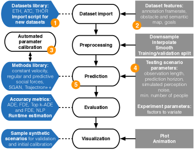
Atlas includes five main elements: data import, preprocessing, the actual prediction phase, evaluation and visualization, see Fig. 1. This design allows to interface and parametrize different prediction algorithms for a flexible and highly automated evaluation and analysis.
As first step, the datasets and, if available, information on the environment such as goals, obstacles, and semantics are imported into the benchmark. Next, the raw data is preprocessed with downsampling to a user-defined frequency, misdetection interpolation and trajectory smoothing. Once the dataset is ready, we extract the testing scenarios with the user-specified observation and prediction lengths, and the minimum number of observed people. The observed past trajectories of all people in the testing scenario, along with environment data, are explicitly interfaced as input to the prediction algorithm. The returned predictions are evaluated against the ground truth using several metrics. Finally, the prediction results can be visualized with plots or animations. Meta-parameters to control the data processing and benchmark setup are stored in separate yaml files, and the benchmark is accessed via Jupyter notebooks.
III-A Datasets
Benchmark users can import any dataset in the specific json file format defined by TrajNet++ [5], which includes for each detection the time stamp, person id and position. The json dataset format also supports obstacles and semantic grid maps [31], as well as goals (i.e. possible destinations of people) in the environment, which may influence the possible destinations of people.
Our benchmark currently includes the following three datasets:
These three datasets come from different countries and were recorded in different environments, which increases the diversity of the scenarios and allows comparing prediction methods on different social and cultural contexts. For an in-depth analysis of the datasets we refer the reader to [16] and [4]. In addition, we provide a possibility to import any dataset of labeled detections, as defined in Sec. II.
III-B Preprocessing
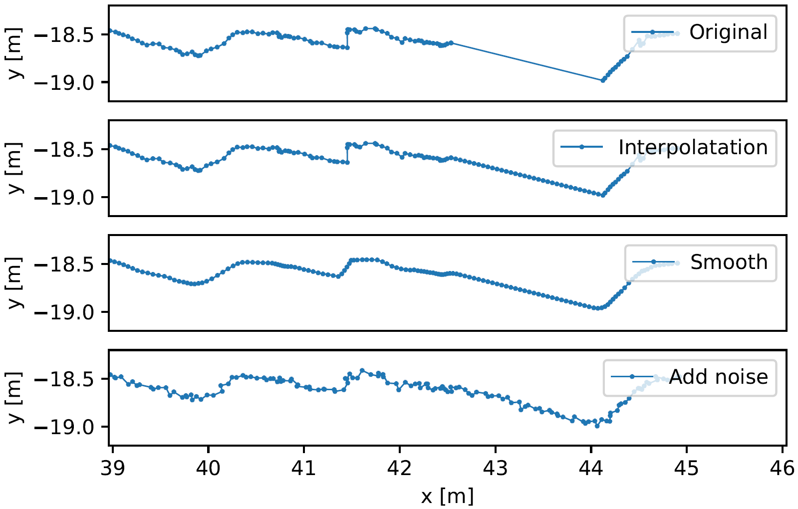
Raw datasets often include noise and annotation artifacts (e.g. missing detections) [16]. Hence, our benchmark offers interpolation and smoothing in the preprocessing step. In addition, as a way to evaluate robustness of prediction algorithms, white Gaussian noise may be added to each detection. Fig. 2 shows the preprocessing steps applied to an example trajectory in the ATC dataset. After detecting the missing frames in the original trajectory based on the average annotation frequency, we interpolate the points linearly in the missing part of the trajectory. Then, a moving average filter is used to smooth the noise. Finally, random noise distributed as , where , can be added to each detection.
After preprocessing, we generate the testing scenarios with the observation length and ground truth for the following frames. As prediction performance may strongly depend on the observation length (in particular for intention estimation or when person detections are noisy), it is critical that all people in the testing scenario are observed in each of the frames. A testing scenario, along with the environment information, is then passed to the prediction step.
III-C Prediction
Our benchmark offers a direct interface to the prediction module, which is called at this step for the given testing scenario. This allows automated evaluation with a systematic variation of parameters, defined at the previous steps. For optimizing the hyperparatemers of the prediction methods, such as [7, 8, 32, 33, 34], Atlas includes an interface to the SMAC3 optimizer [6].
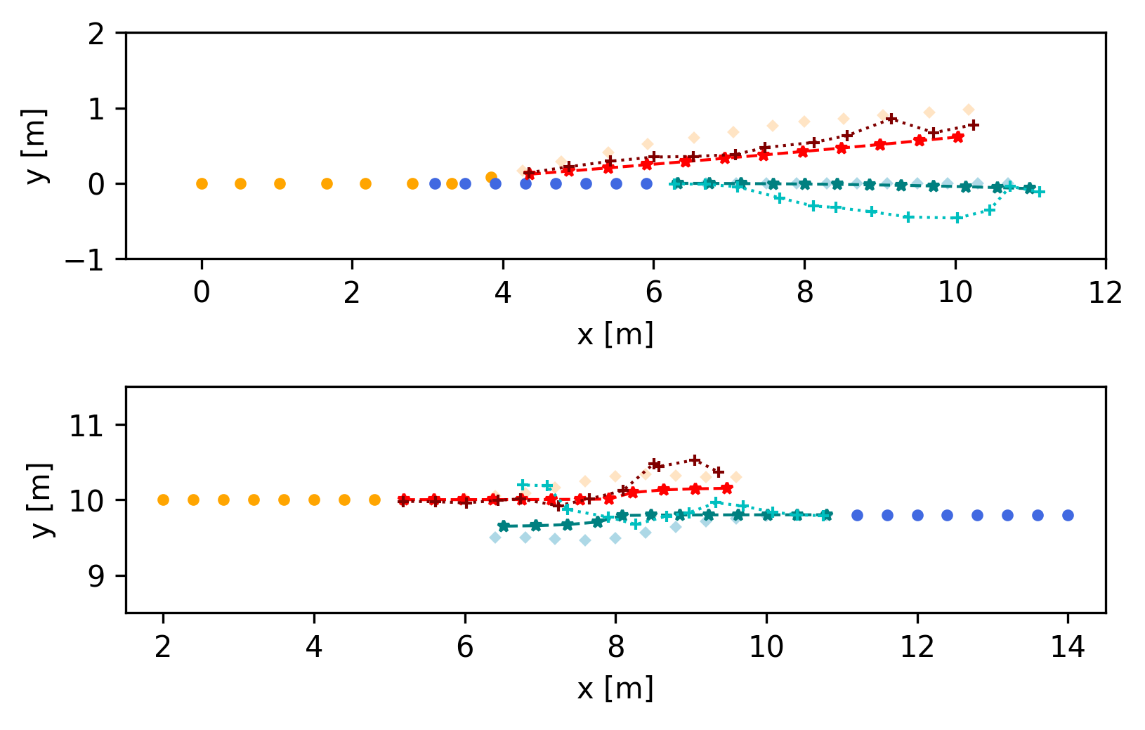
Prior to benchmarking the prediction model on real data, the users can first validate their methods with several synthetic scenarios, which model fundamental interactions between people and the environment, e.g. individuals and groups walking in the opposite directions, crossing paths and navigating around hindrances (see several examples in Fig. 3). For instance, Fig. 3 (bottom left) shows two people walking on a collision course towards each other. Their velocities are 1 and the initial displacement in the axis is 0.2 . The frame frequency is and is 8 (frames).
Our benchmark supports various forms of parametric and non-parametric uncertainty representations for the prediction results. Non-parametric particle-based uncertain predictions are represented with a set of discrete sampled positions for each timestep. Alternatively, the results can be encoded as probabilities in 2D grid-map states, separately for each person in each timestep. Parametric uncertainty can be represented with a mixture of Gaussians: each individual mode of motion is given as a sequence of Gaussian distributions , and the full predicted probability for timestep is , where are the mixture weights. These options allow the evaluation of most existing prediction algorithms.
III-D Evaluation
The Atlas benchmark supports geometric and probabilistic metrics, as defined in [4]. Geometric metrics include the Average Displacement Error (ADE), which describes the error between points of predicted trajectories and the ground truth at the same timestep, and the Final Displacement Error (FDE), which computes the error at the last prediction step. Probabilistic metrics include the Negative Log-Probability (NLP), which computes the average probability of the ground truth position under the predicted distribution for the corresponding frame, and Top-k ADE and FDE, which compute the displacements between the ground truth position and the closest of the samples from the predicted distribution.
III-E Experiments
Building on the datasets, pre-processing steps and metrics described above, the benchmark enables researchers to set up and conduct several experiments to study prediction performance under varying conditions. Such experiments are not only key for researchers to better understand the algorithm or model at hand, e.g. during ablation studies, but also for practitioners to evaluate a predictor within a system with adjacent up- and downstream tasks and real-world deployments.
III-E1 Prediction accuracy conditioned on parameters
and are among the main factors, associated with predicting motion. The accuracy naturally degrades for further time instances, while longer observations may improve it overall. In Atlas it is possible to measure the accuracy of prediction conditioned on these two main parameters. Further accuracy breakdown is possible by conditioning the measured values on the number of people in the scenario.
III-E2 Transfer experiments
A crucial part of evaluating a prediction method is to analyze its generalization ability to new environments not included in the training data. Such experiments are most often overlooked in related work. In Atlas it is possible to script hyperparameter optimization in one dataset, and evaluate the method in another. In the future we plan to extend this functionality for training models.
III-E3 Robustness experiments
For a system to work in the real world, a predictor must be robust against imperfection in perception such as noisy agent position observations. One possible way to quantify robustness, implemented in Atlas, is by measuring accuracy on the testing scenarios, after artificially adding increasing amounts of white Gaussian noise.
IV Example Evaluation
With the Atlas benchmark described above, we now demonstrate its usage in an example evaluation. To this end, we conducted experiments to study and compare the performance of a small range of popular methods for human motion prediction, from simple physics-based baselines to state-of-the-art deep learning methods.
IV-A Prediction methods
Our benchmark comes with several model- and learning-based methods [7, 8, 32, 9, 10]. The Social force model [7] (Sof) is a simple and well-known approach to interaction modeling of people in groups, used in applications such as crowd behavior analysis, simulation and animation [35, 34], robotics [36] and human motion prediction [37]. We also consider the extension of the social force model by Karamouzas et al. [8] (Kara) who added a predictive ability to the initial approach by forward projection of the agent’s current motion and avoiding collisions in advance. The constant velocity motion model (CVM) further serves as baseline in our experiments.
The shift towards learning-based methods for human motion prediction has produced a large number of new methods and models in recent years. For our example comparison, we include two state-of-the-art methods, Trajectron++ [10] (T++), a graph-structured generative neural network based on a conditional-variational autoencoder and Social GAN [9] (SGAN), which combines a recurrent sequence-to-sequence model with a generative adversarial network.
IV-B Setup
In our evaluation we vary the testing parameters around the commonly used values of and . As all datasets in our experiments are downsampled to , this implies and . This is the standard setup in all experiments in ATC and THÖR, where one parameter (for instance , , the amount of added noise , calibration/validation datasets) is varied. Due to the limited number of data in ETH, we set and (equivalent to and ) instead. To stress the agent interaction aspect of motion prediction, scenarios with less than 2 people are excluded from the evaluation. We report the mean and standard deviation of the ADE and FDE metrics across all scenarios in the experiment.
The force-based methods (Sof and Kara) are optimized separately in each dataset on the initial 30% of the detections (20% in case of ETH). The target optimization metric is FDE at . For the optimization parameters of each individual method, we refer the reader to the provided implementations. The current velocity of each person , used as input to the force-based methods and the CVM, is calculated as a weighted sum of the finite differences in the observed trajectories. The sequence of past velocities is weighted with a zero-mean Gaussian filter with to put more weight on the more recent observations: , where . The goal of each person is set to the point reached by forward propagating 40 steps into the future with .
The Trajectron++ implementation is accessed from the official repository777https://github.com/StanfordASL/Trajectron-plus-plus, for which we provide a lightweight interface. This predictor is trained on the ETH dataset. We sample Trajectron++ once to get the most likely predicted trajectory.
For the Social GAN we use the implementation provided by the authors888https://github.com/agrimgupta92/sgan. The model is trained on the ETH dataset, and is limited to accepting 8 frames as observations and producing 12 frames of prediction. Therefore, we exclude it from all experiments with and . Similarly to T++, we sample SGAN for one mode.
| Prediction horizon | |||||
| Method | 1.6 s | 3.2 s | 4.8 s | 8 s | |
| ADE | CVM | ||||
| Sof | |||||
| Kara | |||||
| SGAN | – | ||||
| T++ | |||||
| FDE | CVM | ||||
| Sof | |||||
| Kara | |||||
| SGAN | – | ||||
| T++ | |||||
| Prediction horizon | |||||
| Method | 1.6 s | 3.2 s | 4.8 s | 8 s | |
| ADE | CVM | ||||
| Sof | |||||
| Kara | |||||
| SGAN | – | ||||
| T++ | |||||
| FDE | CVM | ||||
| Sof | |||||
| Kara | |||||
| SGAN | – | ||||
| T++ | |||||
In addition to the accuracy measurements under various conditions, we also estimate the prediction runtime conditioned on the number of people in the scenario. All experiments were executed on a laptop with an Intel i7 2.7 GHz 12 core processor and 32 GB of RAM.
Note that the evaluation results may differ from the original papers [1, 9, 10], due to the differences in the evaluation protocols, which are not fully disclosed and therefore not reproducible. This particularly highlights the need for standardized benchmarks like Atlas, which allow for transparent verification of reported results and direct comparisons of methods under various conditions of interest.
IV-C Results and Discussion
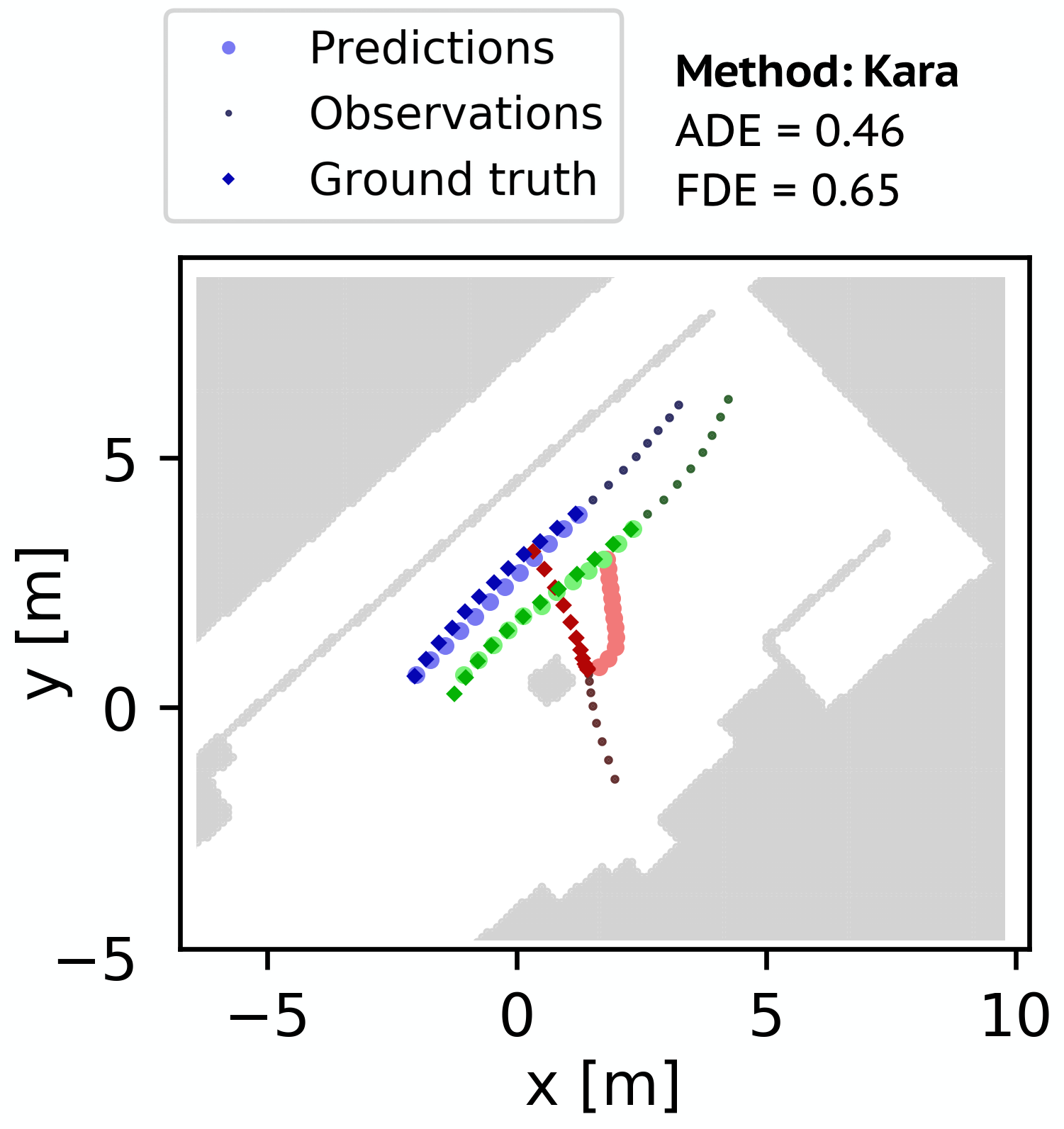
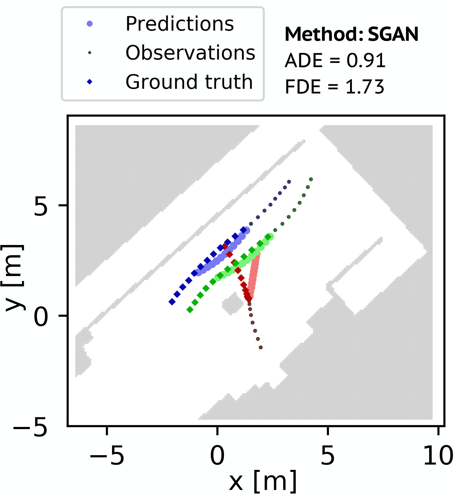
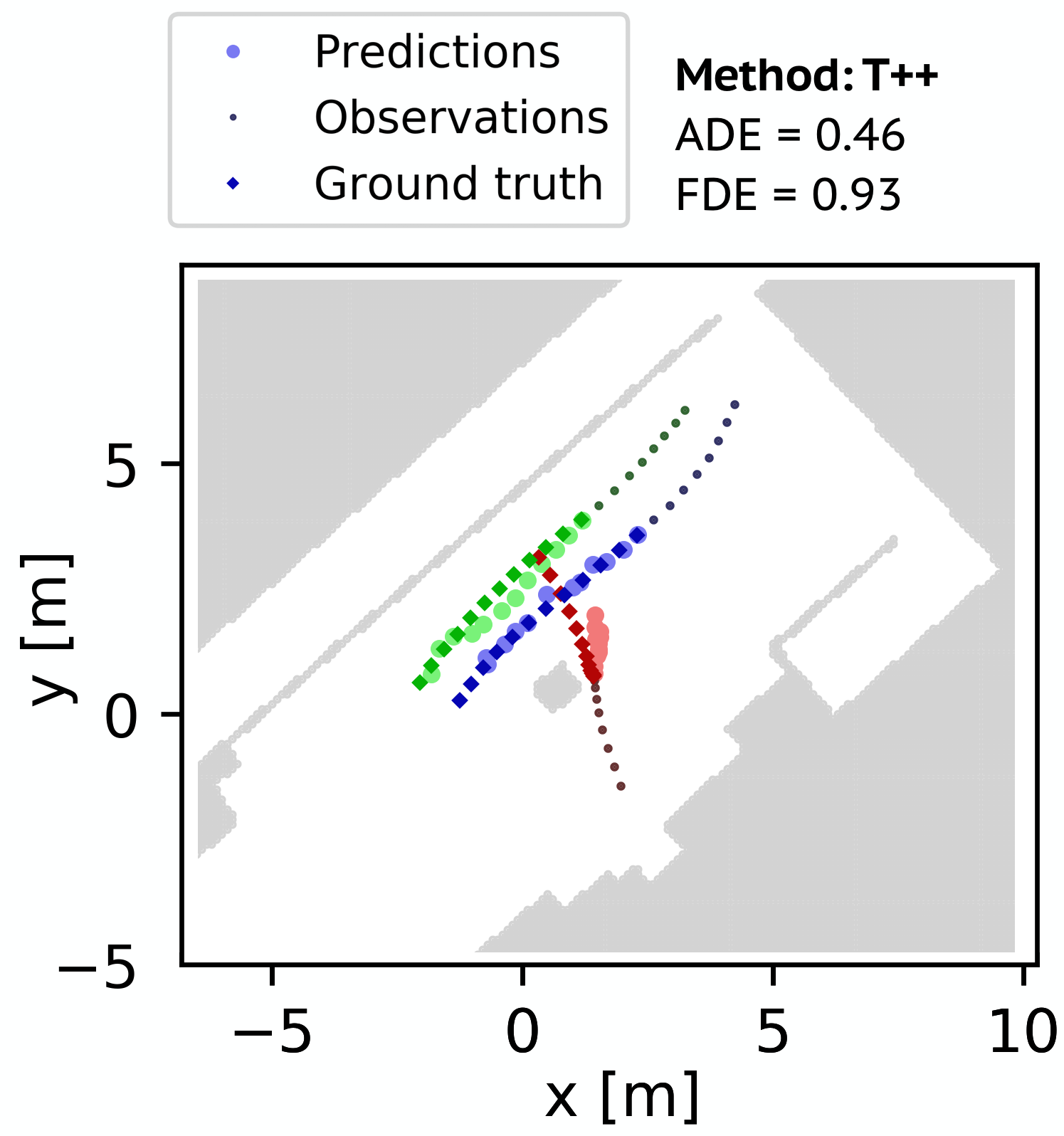
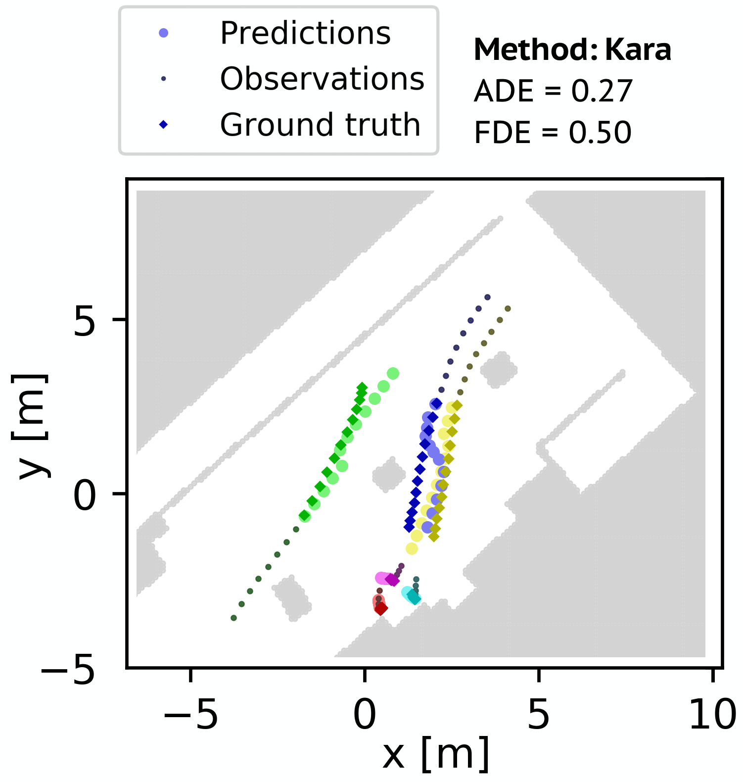
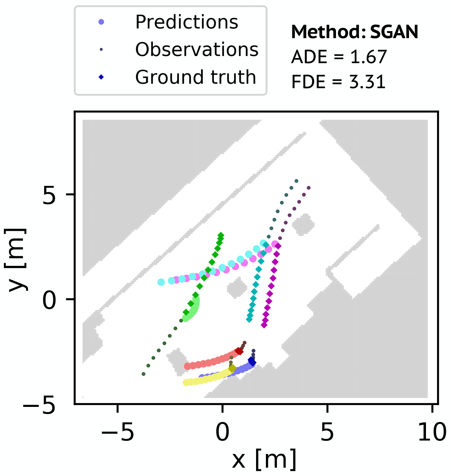
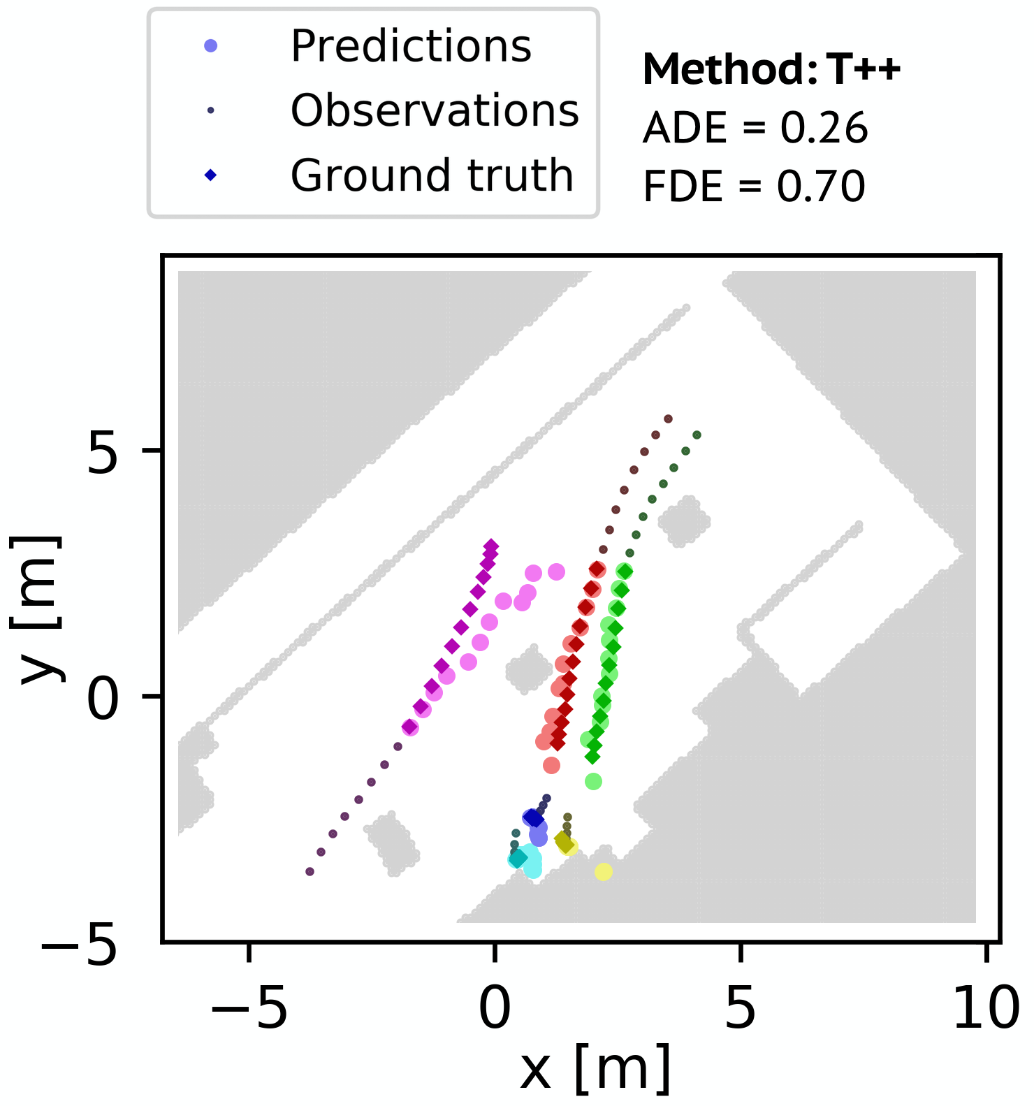
We present the results in Tables I–III, Fig. 4–8 and show example predictions in Fig. 9–12. Due to space limitations, results of each experiment are presented in selected datasets only, but the discussed trends are observed in all of them.
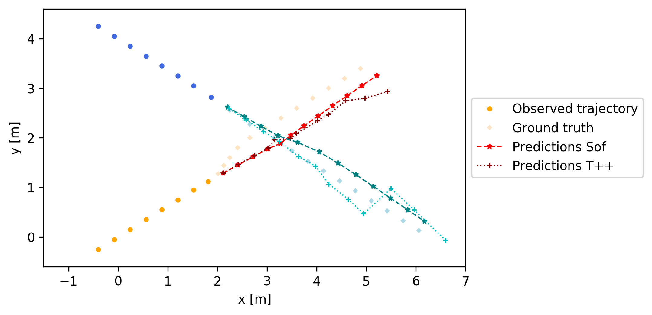
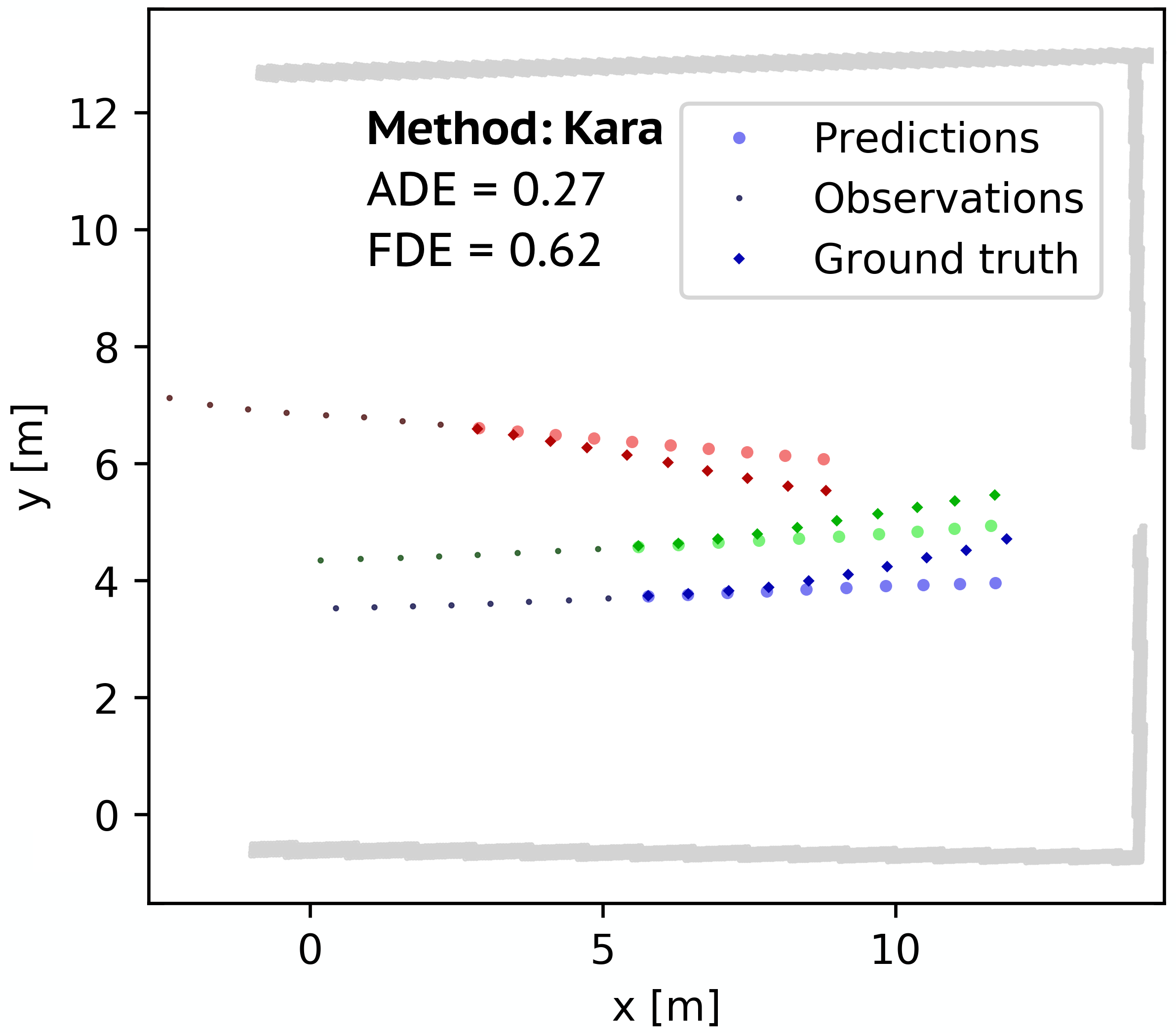
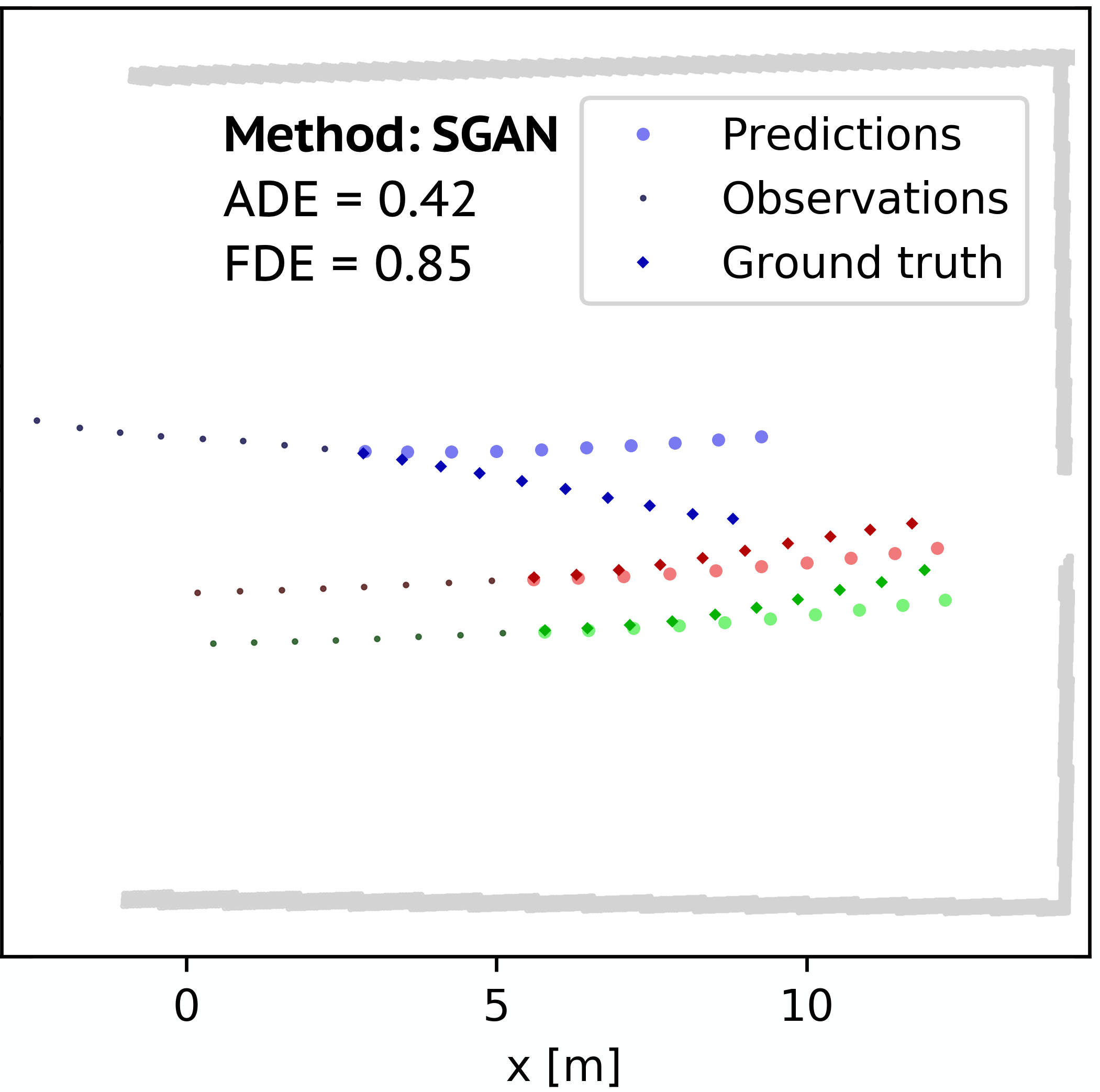
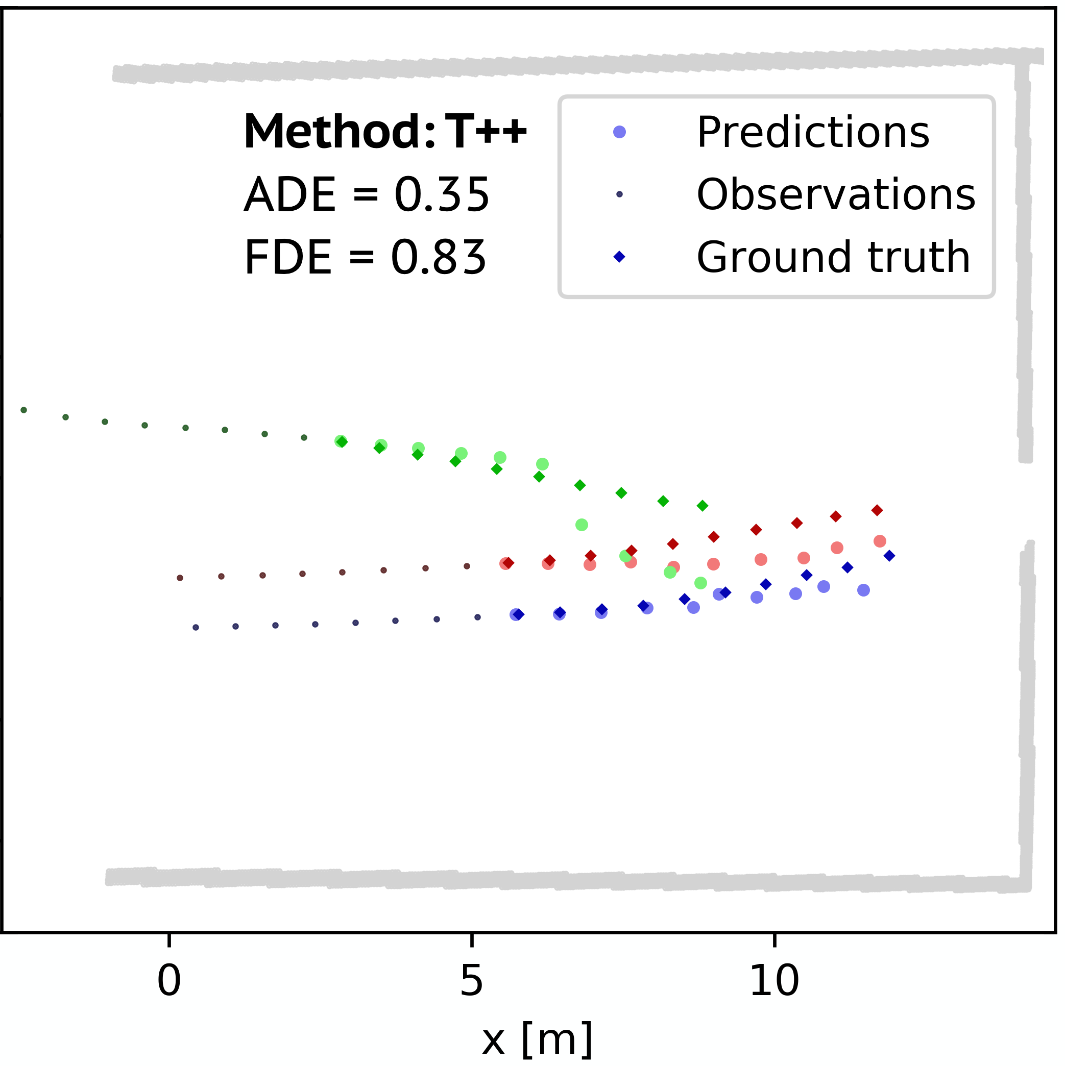
Tables I and II show the results of evaluating the ADE and FDE on different prediction horizons with the fixed observation period . In the ATC dataset, which contains mostly straight linear motion, even in crowded scenes, the force-based approaches perform on the level of constant velocity. Trajectron++ and SGAN, on the other hand, attempt to predict more variety in motion than what exists in real life, leading to higher displacement errors (see an example scenario in Fig. 10).
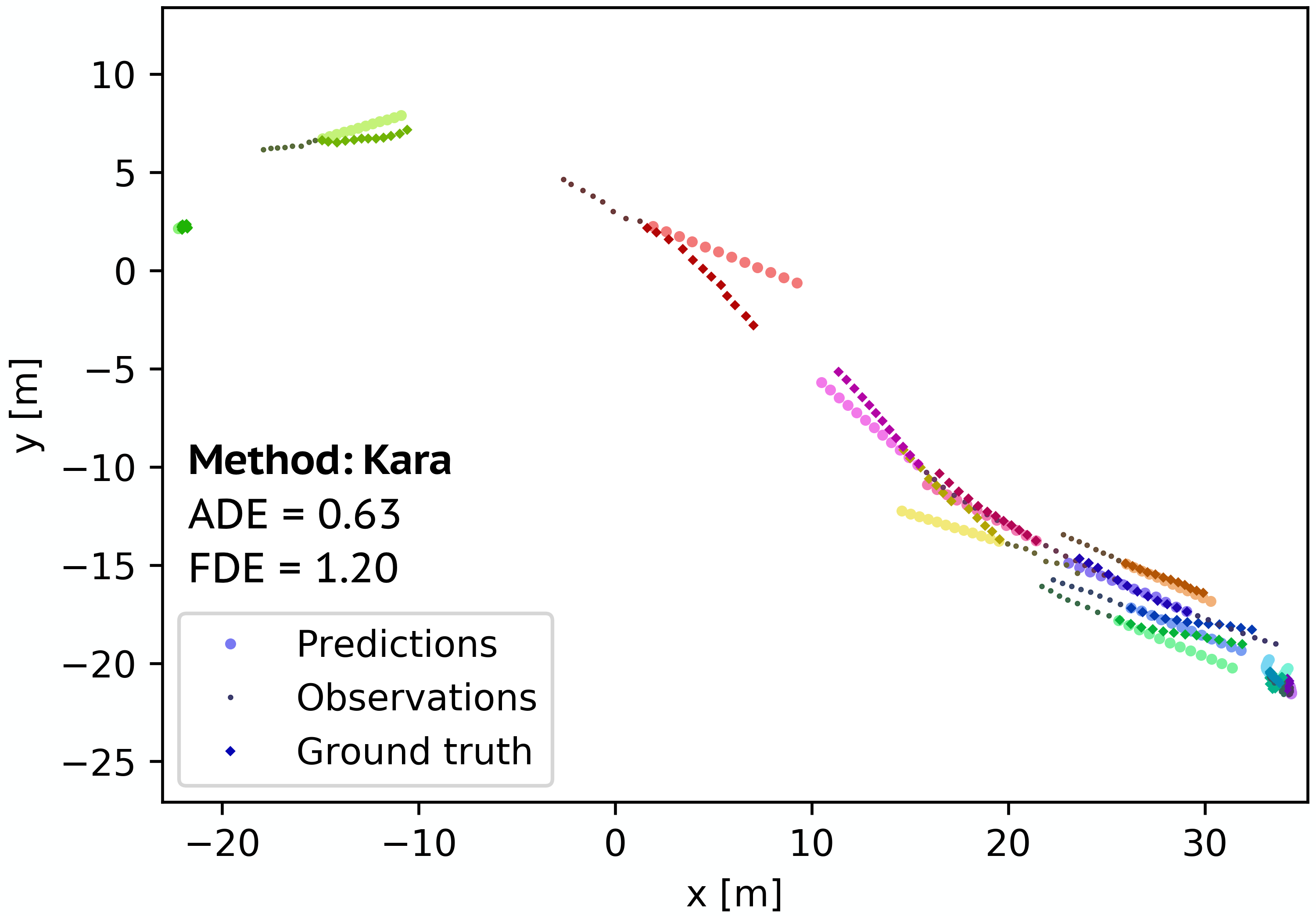
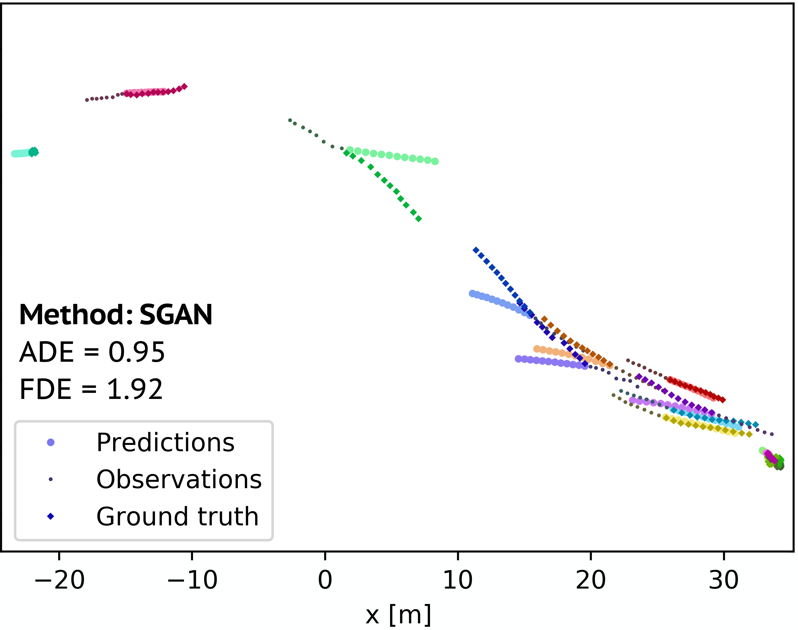
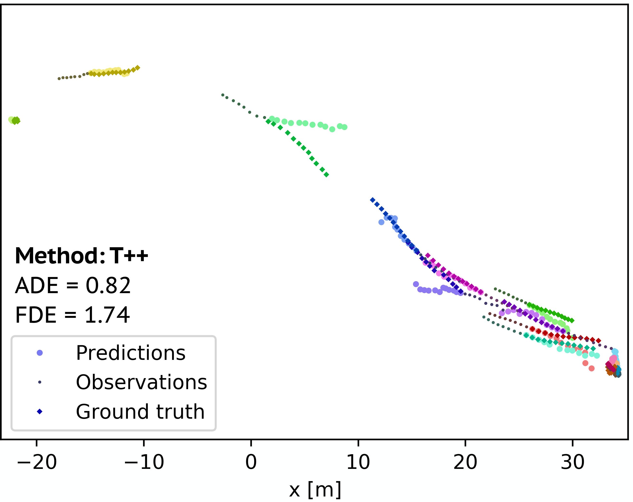
In the THÖR3 dataset (Table II and Fig. 12), on the contrary, people navigate in a tighter environment across multiple directions, increasing the importance of good interaction modeling. Here Trajectron++ outperforms the CVM, however the best and most stable results are reached by the force-based methods.
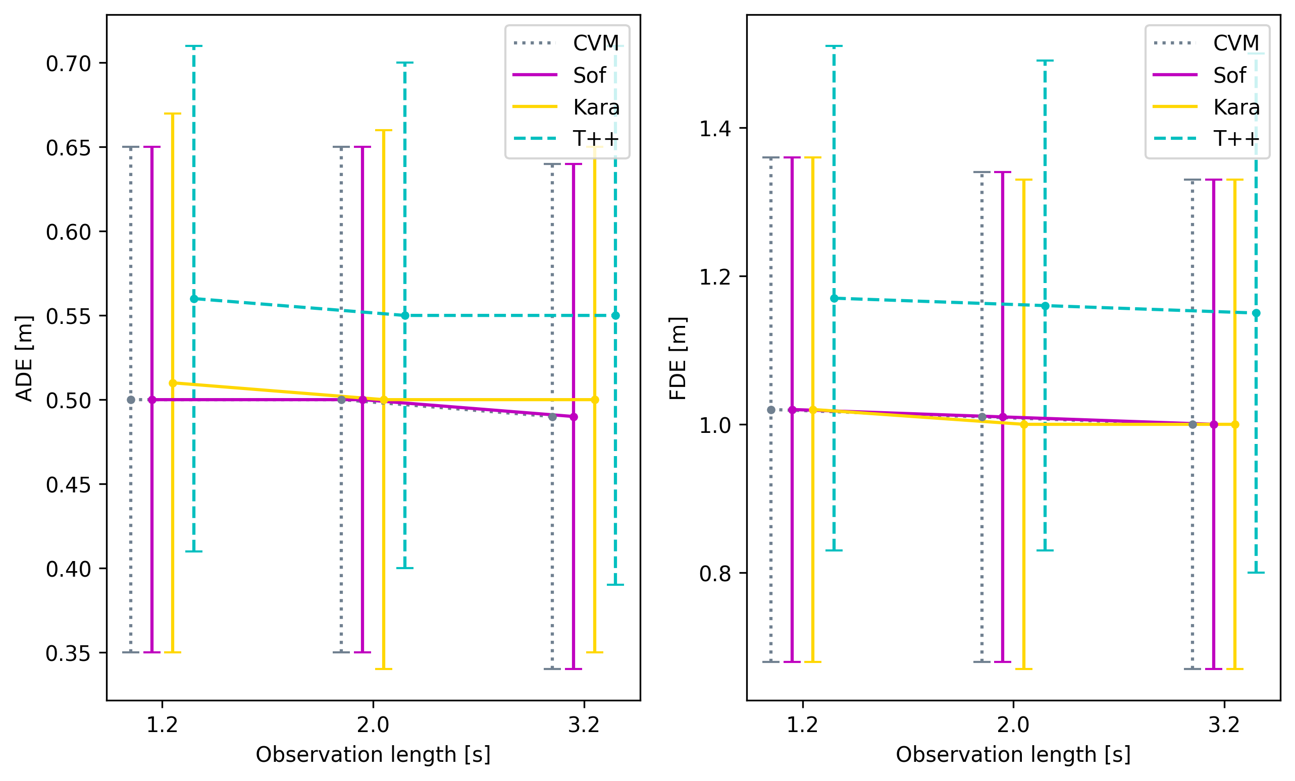
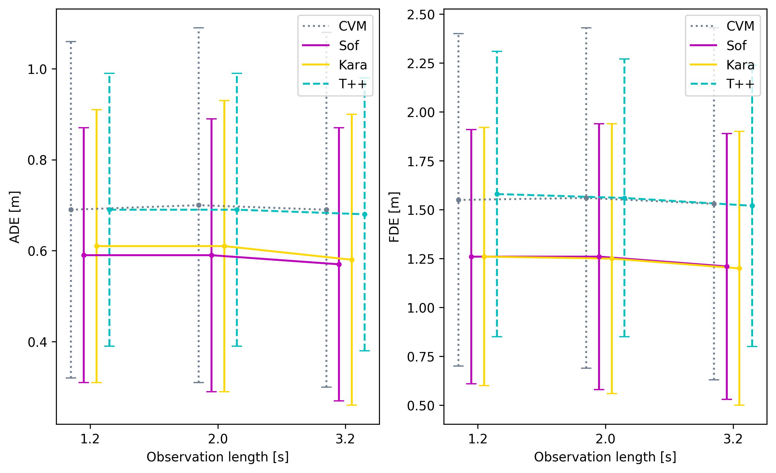
In the experiments with different observation horizons we found all methods to perform very robustly even with observation lengths as short as 1.2 , see Fig. 4 and 5. The ADE/FDE results for increasing amounts of noise in the agent positions added to the ETH and THÖR3 data are shown in Fig. 6 and 7. The performance of all methods, including Trajectron++, degrades considerably when the observations become more unreliable (with ) where SGAN shows an almost linear degradation to the amount of noise, as compared to exponential decrease of other methods. Again, the model-based methods outperform the learning-based ones.
| Test | |||||
|---|---|---|---|---|---|
| Calibrate | Dataset | ETH | ATC | THÖR1 | THÖR3 |
| ETH | CVM: Sof: Kara: SGAN: T++: | ||||
| ATC | Sof: Kara: | ||||
| THÖR1 | Sof: Kara: | ||||
| THÖR3 | Sof: Kara: | ||||
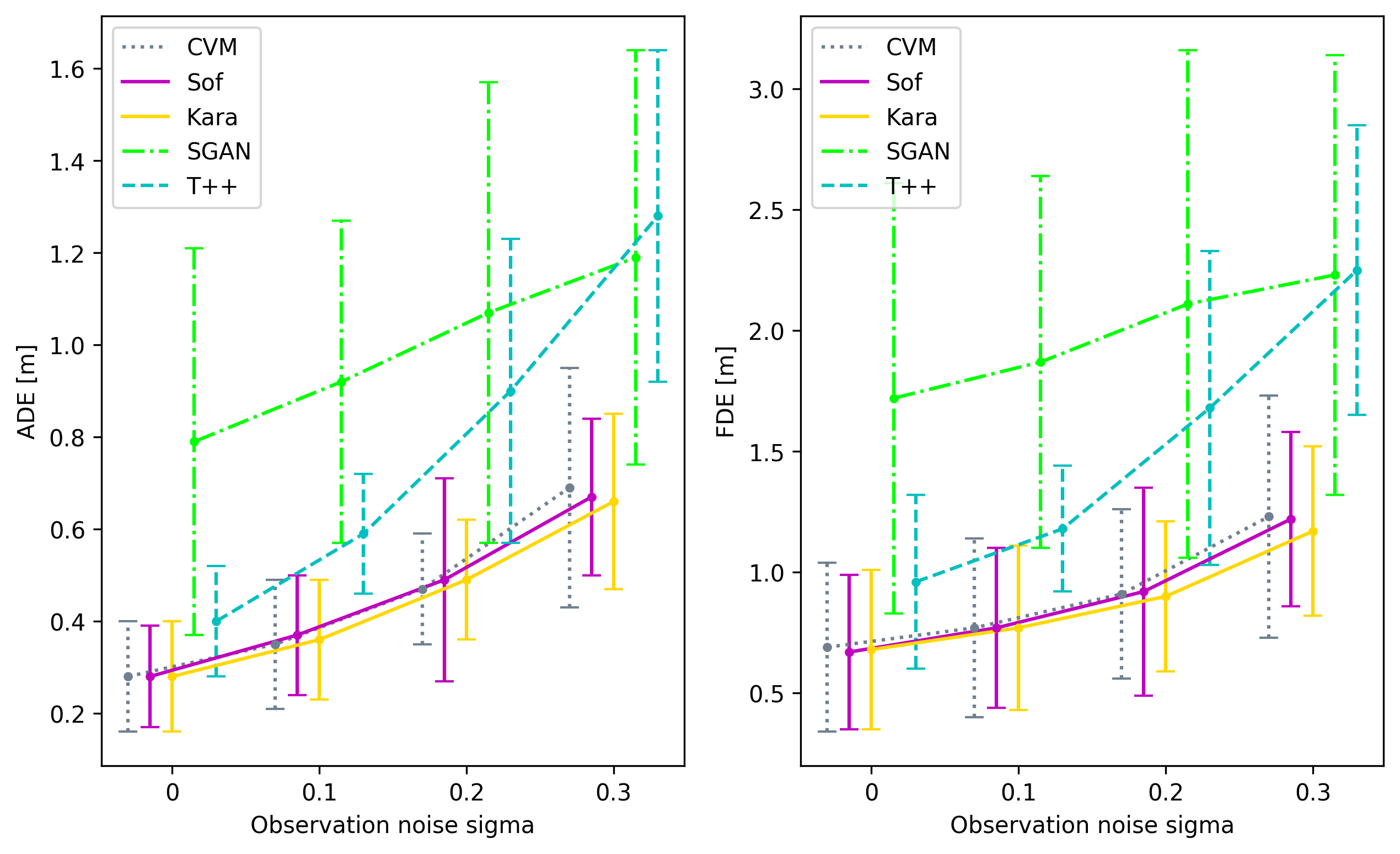
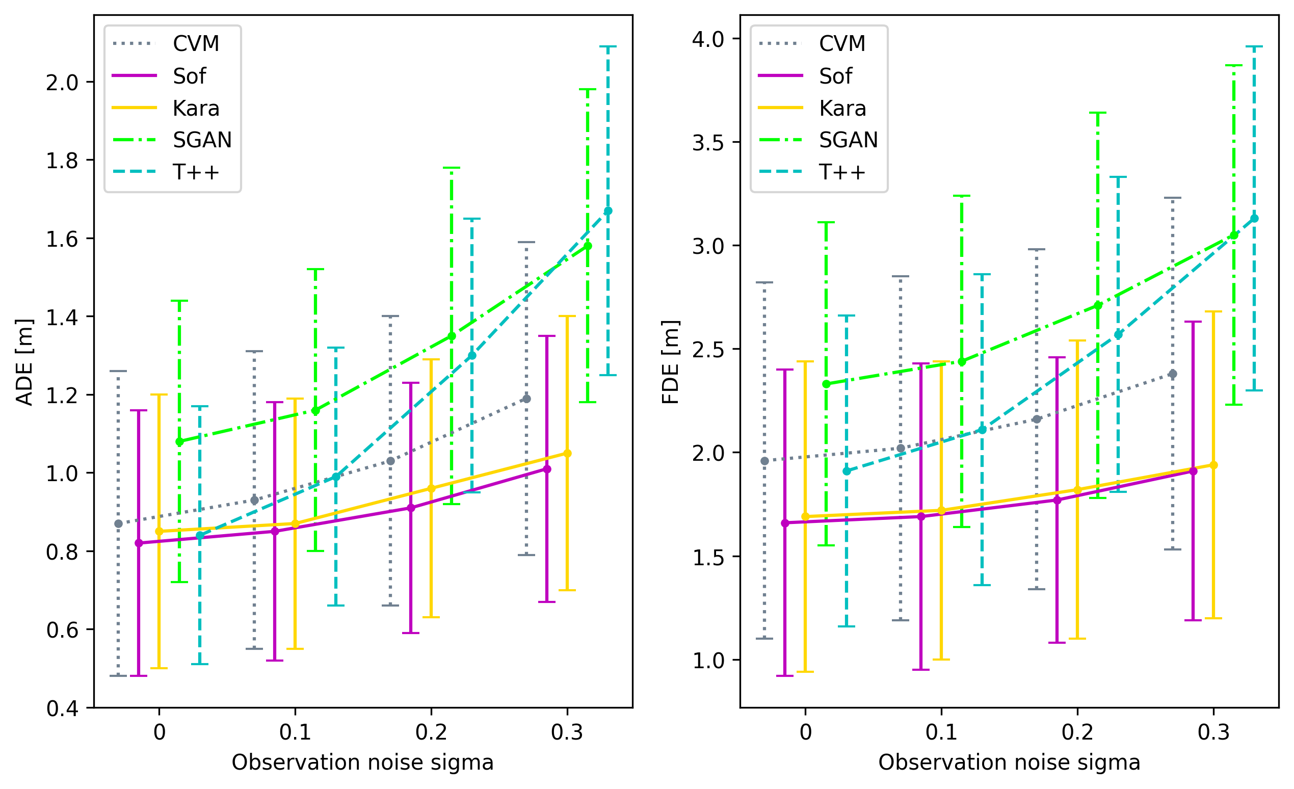
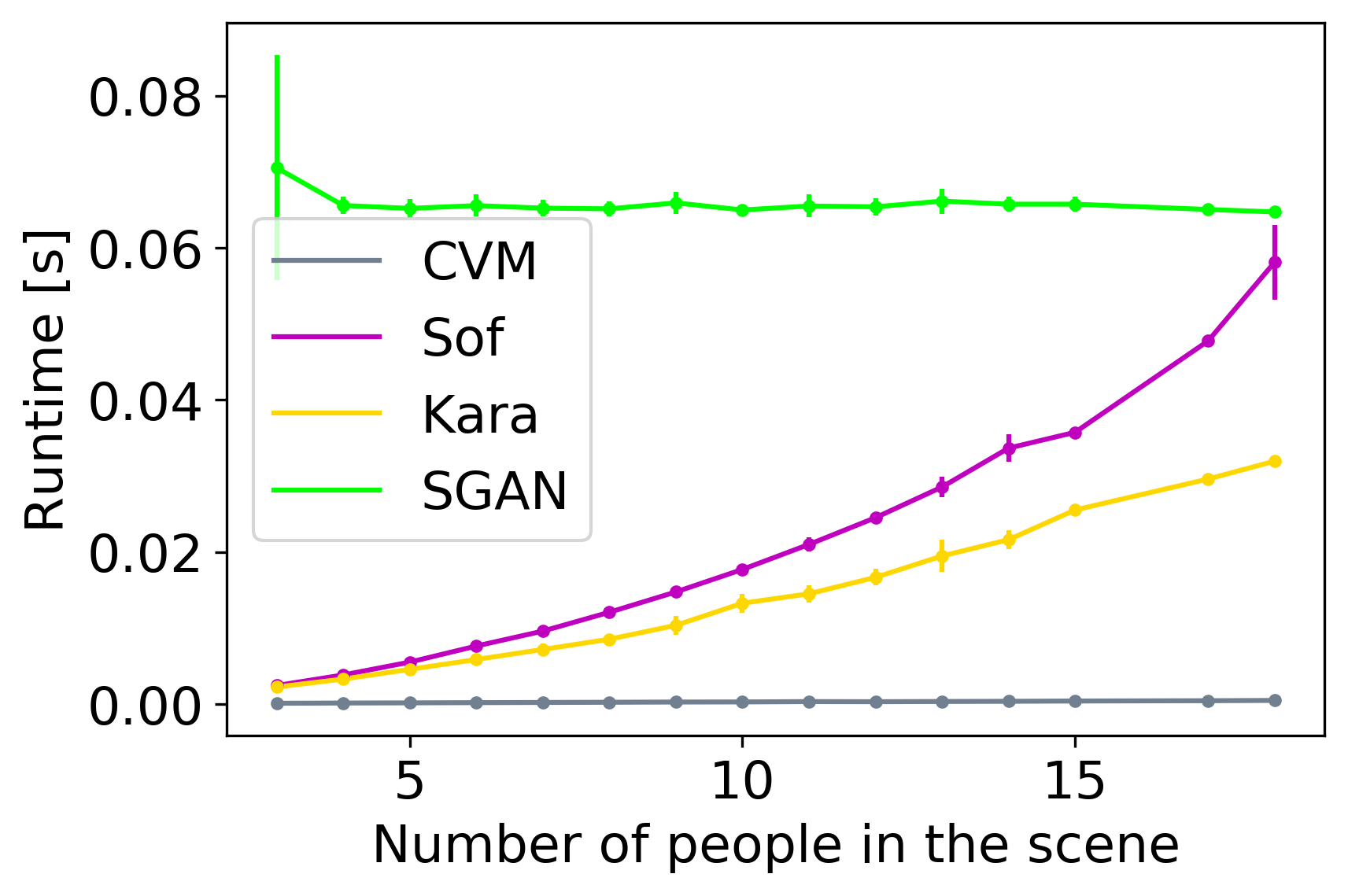
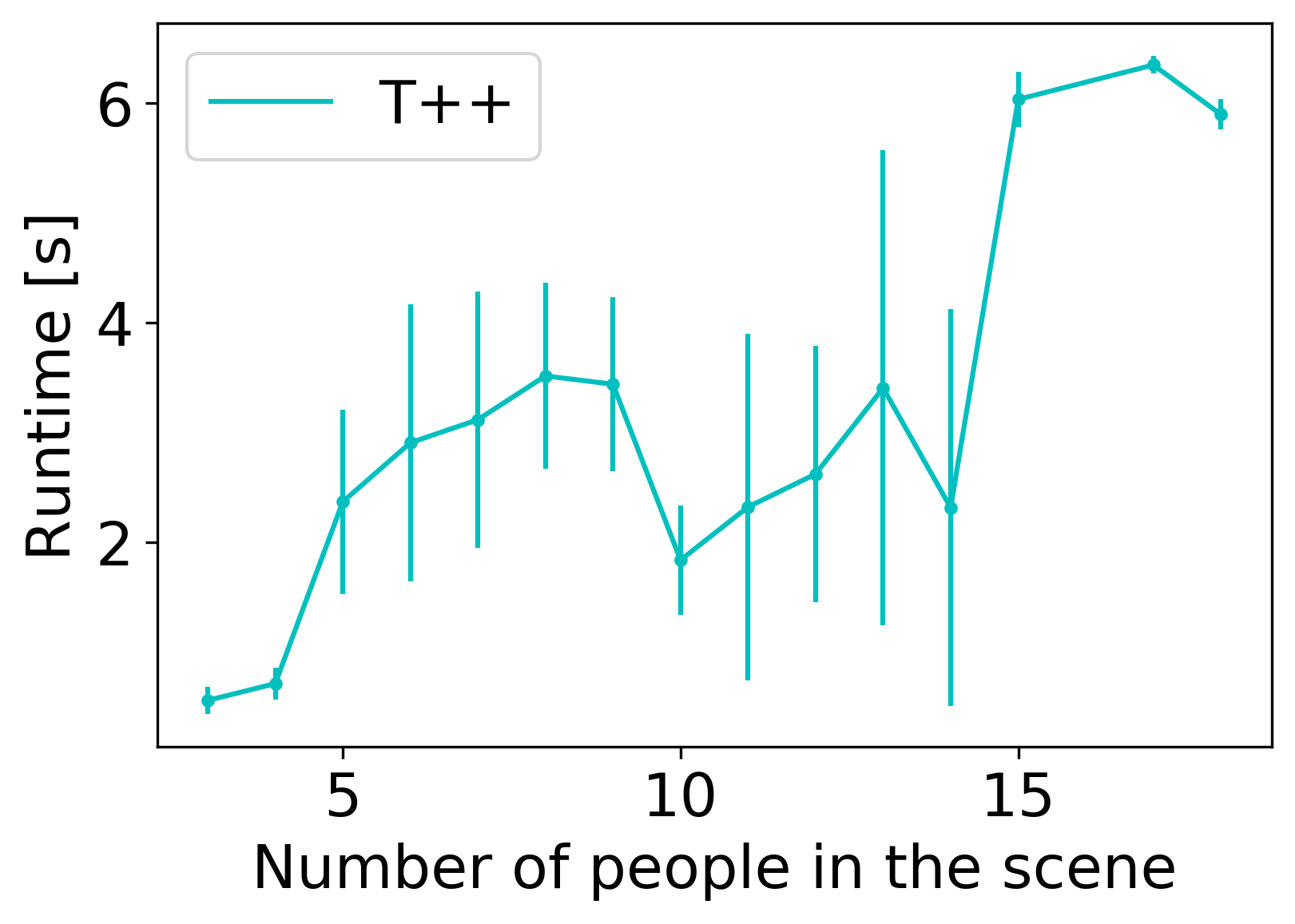
Table III summarizes the transfer experiment, where the methods are calibrated on one dataset and tested on another. We observe that the predictive social force approach (Kara) delivers more stable transfer performance in all cases as compared to the Sof method.
An overall conclusion from the experiments, supported by the qualitative analysis in Fig. 9–12, is that the model-based prediction methods, properly calibrated, with velocity filtering and goal projection, offer a surprisingly competitive alternative to the complex state-of-the-art deep learning approaches. This result seems to confirm the recent findings by Schöller et al. [2], once again indicating that learning interactions is an extremely challenging task prone to evaluation pitfalls. That, and the considerable runtime differences in favor of the model-based approaches in Fig. 8, justifies the need for further research into interaction models, both engineered and learned ones. Another conclusion is that, in our experiments, the predictive social force model does not reliably outperform the original method. Finally, the results of the force-based methods calibrated on simpler datasets with a lot of linear motion (such as the ETH and ATC) converge to the CVM model up to the 3rd decimal digit (i.e. less than 1 difference).
V Summary and Future Work
The number of approaches for human motion prediction has grown rapidly in recent years but different datasets and varying evaluation protocols make in-depth analysis and comparisons difficult. This is the motivation for Atlas, introduced in this paper, an evaluation benchmark for motion prediction that enables researchers to analyze and compare their methods in an unified easy-to-use framework. Unlike related benchmarks and challenges, Atlas offers data preprocessing functions, hyperparameter optimization, three popular datasets and the fexibility to setup and conduct underexplored yet relevant experiments to stress a method’s accuracy and robustness. In an example application of Atlas, we compared five popular prediction methods, three early physics-based approaches and two learning-based state-of-the-art approaches and found that the model-based methods, properly applied, are surprisingly competitive. While these findings motivate further research particularly in agent interaction modeling, they also show the necessity for such benchmarks to reproduce, confirm and further extend such results.
In future work we intend to extend Atlas with support for more datasets, more baselines, more motion cues such as group motion or articulated body pose, non-human dynamic agents such as vehicles or robots and other relevant environment descriptors, e.g. maps of dynamics [38]. Furthermore, considering the downstream performance metrics in how the predictions affect the robot behavior, we seek to close the loop on the human motion prediction benchmarking by connecting it to robot navigation simulation [39].
References
- [1] A. Alahi, K. Goel, V. Ramanathan, A. Robicquet, L. Fei-Fei, and S. Savarese, “Social LSTM: Human trajectory prediction in crowded spaces,” in Proc. of the IEEE Conf. on Comp. Vis. and Pat. Rec. (CVPR), 2016, pp. 961–971.
- [2] C. Schöller, V. Aravantinos, F. Lay, and A. Knoll, “What the constant velocity model can teach us about pedestrian motion prediction,” IEEE Robotics and Automation Letters, vol. 5, no. 2, pp. 1696–1703, 2020.
- [3] S. Becker, R. Hug, W. Hubner, and M. Arens, “Red: A simple but effective baseline predictor for the trajnet benchmark,” in Proc. of the Europ. Conf. on Comp. Vision (ECCV) Workshops, 2018.
- [4] A. Rudenko, L. Palmieri, M. Herman, K. M. Kitani, D. M. Gavrila, and K. O. Arras, “Human motion trajectory prediction: A survey,” Int. J. of Robotics Research, vol. 39, no. 8, pp. 895–935, 2020.
- [5] P. Kothari, S. Kreiss, and A. Alahi, “Human trajectory forecasting in crowds: A deep learning perspective,” IEEE Trans. on Intell. Transp. Syst. (TITS), 2021.
- [6] M. Lindauer, K. Eggensperger, M. Feurer, S. Falkner, A. Biedenkapp, and F. Hutter, “Smac v3: Algorithm configuration in python,” https://github.com/automl/SMAC3, 2017.
- [7] D. Helbing and P. Molnar, “Social force model for pedestrian dynamics,” Physical review E, vol. 51, no. 5, p. 4282, 1995.
- [8] I. Karamouzas, P. Heil, P. van Beek, and M. H. Overmars, “A predictive collision avoidance model for pedestrian simulation,” in Int. Workshop on Motion in Games. Springer, 2009, pp. 41–52.
- [9] A. Gupta, J. Johnson, L. Fei-Fei, S. Savarese, and A. Alahi, “Social GAN: Socially acceptable trajectories with generative adversarial networks,” in Proc. of the IEEE Conf. on Comp. Vis. and Pat. Rec. (CVPR), June 2018.
- [10] T. Salzmann, B. Ivanovic, P. Chakravarty, and M. Pavone, “Trajectron++: Dynamically-feasible trajectory forecasting with heterogeneous data,” in European Conference on Computer Vision. Springer, 2020, pp. 683–700.
- [11] S. Pellegrini, A. Ess, K. Schindler, and L. van Gool, “You’ll never walk alone: Modeling social behavior for multi-target tracking,” in Proc. of the IEEE Int. Conf. on Computer Vision (ICCV), 2009, pp. 261–268.
- [12] A. Lerner, Y. Chrysanthou, and D. Lischinski, “Crowds by example,” in Computer Graphics Forum, vol. 26, no. 3. Wiley Online Library, 2007, pp. 655–664.
- [13] B. Majecka, “Statistical models of pedestrian behaviour in the forum,” Master’s thesis, School of Informatics, University of Edinburgh, 2009.
- [14] D. Brščić, T. Kanda, T. Ikeda, and T. Miyashita, “Person tracking in large public spaces using 3-d range sensors,” IEEE Trans. on Human-Machine Systems, vol. 43, no. 6, pp. 522–534, 2013.
- [15] A. Robicquet, A. Sadeghian, A. Alahi, and S. Savarese, “Learning social etiquette: Human trajectory understanding in crowded scenes,” in Proc. of the Europ. Conf. on Comp. Vision (ECCV). Springer, 2016, pp. 549–565.
- [16] A. Rudenko, T. P. Kucner, C. S. Swaminathan, R. T. Chadalavada, K. O. Arras, and A. J. Lilienthal, “THÖR: Human-robot navigation data collection and accurate motion trajectories dataset,” IEEE Robotics and Automation Letters, vol. 5, no. 2, pp. 676–682, 2020.
- [17] A. Sadeghian, V. Kosaraju, A. Gupta, S. Savarese, and A. Alahi, “TrajNet: Towards a benchmark for human trajectory prediction,” arXiv preprint, 2018.
- [18] A. Sadeghian, V. Kosaraju, A. Sadeghian, N. Hirose, and S. Savarese, “SoPhie: An attentive GAN for predicting paths compliant to social and physical constraints,” in Proc. of the IEEE Conf. on Comp. Vis. and Pat. Rec. (CVPR), 2019, pp. 1349–1358.
- [19] Y. Huang, H. Bi, Z. Li, T. Mao, and Z. Wang, “STGAT: Modeling spatial-temporal interactions for human trajectory prediction,” in Proc. of the IEEE Int. Conf. on Computer Vision (ICCV), 2019, pp. 6272–6281.
- [20] V. Kosaraju, A. Sadeghian, R. Martín-Martín, I. Reid, H. Rezatofighi, and S. Savarese, “Social-bigat: Multimodal trajectory forecasting using bicycle-gan and graph attention networks,” Advances in Neural Inf. Proc. Syst. (NIPS), vol. 32, 2019.
- [21] N. Nikhil and B. Tran Morris, “Convolutional neural network for trajectory prediction,” in Proc. of the Europ. Conf. on Comp. Vision (ECCV), 2018.
- [22] M. Huynh and G. Alaghband, “Trajectory prediction by coupling scene-LSTM with human movement LSTM,” in Int. Symposium on Visual Computing. Springer, 2019, pp. 244–259.
- [23] H. Xue, D. Q. Huynh, and M. Reynolds, “SS-LSTM: a hierarchical LSTM model for pedestrian trajectory prediction,” in Proc. of the IEEE Winter Conf. on Applications of Computer Vision (WACV). IEEE, 2018, pp. 1186–1194.
- [24] T. Zhao, Y. Xu, M. Monfort, W. Choi, C. Baker, Y. Zhao, Y. Wang, and Y. N. Wu, “Multi-agent tensor fusion for contextual trajectory prediction,” in Proc. of the IEEE Conf. on Comp. Vis. and Pat. Rec. (CVPR), 2019, pp. 12 126–12 134.
- [25] P. Zhang, W. Ouyang, P. Zhang, J. Xue, and N. Zheng, “SR-LSTM: State refinement for LSTM towards pedestrian trajectory prediction,” in Proc. of the IEEE Conf. on Comp. Vis. and Pat. Rec. (CVPR), 2019, pp. 12 085–12 094.
- [26] J. Amirian, J.-B. Hayet, and J. Pettré, “Social ways: Learning multi-modal distributions of pedestrian trajectories with GANs,” in Proc. of the IEEE Conf. on Comp. Vis. and Pat. Rec. (CVPR) Workshops, 2019.
- [27] F. Bartoli, G. Lisanti, L. Ballan, and A. D. Bimbo, “Context-aware trajectory prediction,” in Proc. of the IEEE Int. Conf. on Pattern Recognition, 2018, pp. 1941–1946.
- [28] T. Fernando, S. Denman, S. Sridharan, and C. Fookes, “Soft+Hardwired attention: An LSTM framework for human trajectory prediction and abnormal event detection,” Neural networks, vol. 108, pp. 466–478, 2018.
- [29] C. Tao, Q. Jiang, L. Duan, and P. Luo, “Dynamic and static context-aware lstm for multi-agent motion prediction,” in Proc. of the Europ. Conf. on Comp. Vision (ECCV). Springer, 2020, pp. 547–563.
- [30] R. Hug, S. Becker, W. Hübner, and M. Arens, “A short note on analyzing sequence complexity in trajectory prediction benchmarks,” 2020.
- [31] A. Rudenko, L. Palmieri, J. Doellinger, A. J. Lilienthal, and K. O. Arras, “Learning occupancy priors of human motion from semantic maps of urban environments,” IEEE Robotics and Automation Letters, vol. 6, no. 2, pp. 3248–3255, 2021.
- [32] F. Zanlungo, T. Ikeda, and T. Kanda, “Social force model with explicit collision prediction,” EPL (Europhysics Letters), vol. 93, no. 6, p. 68005, 2011.
- [33] S. Kim, S. J. Guy, W. Liu, D. Wilkie, R. W. H. Lau, M. C. Lin, and D. Manocha, “BRVO: Predicting pedestrian trajectories using velocity-space reasoning,” Int. J. of Robotics Research, vol. 34, no. 2, pp. 201–217, 2015.
- [34] F. Farina, D. Fontanelli, A. Garulli, A. Giannitrapani, and D. Prattichizzo, “Walking ahead: The headed social force model,” PloS one, vol. 12, no. 1, p. e0169734, 2017.
- [35] X. Yang, H. Dong, Q. Wang, Y. Chen, and X. Hu, “Guided crowd dynamics via modified social force model,” Physica A: Statistical Mechanics and its Applications, vol. 411, pp. 63–73, 2014.
- [36] M. Luber, J. A. Stork, G. D. Tipaldi, and K. O. Arras, “People tracking with human motion predictions from social forces,” in Proc. of the IEEE Int. Conf. on Robotics and Automation (ICRA), 2010, pp. 464–469.
- [37] A. Rudenko, L. Palmieri, and K. O. Arras, “Joint prediction of human motion using a planning-based social force approach,” in Proc. of the IEEE Int. Conf. on Robotics and Automation (ICRA), 2018, pp. 1–7.
- [38] T. P. Kucner, A. J. Lilienthal, M. Magnusson, L. Palmieri, and C. S. Swaminathan, Probabilistic mapping of spatial motion patterns for mobile robots. Springer, 2020.
- [39] E. Heiden, L. Palmieri, L. Bruns, K. O. Arras, G. S. Sukhatme, and S. Koenig, “Bench-mr: A motion planning benchmark for wheeled mobile robots,” IEEE Robotics and Automation Letters, vol. 6, no. 3, pp. 4536–4543, 2021.