Anatomy of rocky planets formed by rapid pebble accretion
III. Partitioning of volatiles between planetary core, mantle,
and atmosphere

Volatile molecules containing hydrogen, carbon, and nitrogen are key components of planetary atmospheres. In the pebble accretion model for rocky planet formation, these volatile species are accreted during the main planetary formation phase. For this study, we modelled the partitioning of volatiles within a growing planet and the outgassing to the surface. The core stores more than 90% of the hydrogen and carbon budgets of Earth for realistic values of the partition coefficients of H and C between metal and silicate melts. The magma oceans of Earth and Venus are sufficiently deep to undergo oxidation of ferrous Fe²⁺ to ferric Fe³⁺. This increased oxidation state leads to the outgassing of primarily CO₂ and H₂O from the magma ocean of Earth. In contrast, the oxidation state of Mars’ mantle remains low and the main outgassed hydrogen carrier is H₂. This hydrogen easily escapes the atmosphere due to the irradiation from the young Sun in XUV wavelengths, dragging with it the majority of the CO, CO₂, H₂O, and N₂ contents of the atmosphere. A small amount of surface water is maintained on Mars, in agreement with proposed ancient ocean shorelines, for moderately low values of the mantle oxidation. Nitrogen partitions relatively evenly between the core and the atmosphere due to its extremely low solubility in magma; the burial of large reservoirs of nitrogen in the core is thus not possible. The overall low N contents of Earth disagree with the high abundance of N in all chondrite classes and favours a volatile delivery by pebble snow. Our model of rapid rocky planet formation by pebble accretion displays broad consistency with the volatile contents of the Sun’s terrestrial planets. The diversity of the terrestrial planets can therefore be used as benchmark cases to calibrate models of extrasolar rocky planets and their atmospheres.

1 Introduction

The delivery of volatiles to the terrestrial planets in the Solar System is traditionally ascribed to impacts of primitive, water-rich asteroids that originated beyond the water ice line (Morbidelli et al., 2000; Raymond & Izidoro, 2017). In this view, the amounts of volatiles such as carbon, nitrogen, and hydrogen are inherently stochastic and could be sourced from a wide range of parent bodies with different isotopic compositions (Marty, 2012; Alexander et al., 2012). This gives the possibility to infer the source population of Earth’s volatiles by comparing, for example, the measured D/H ratio of Earth to that of various meteorite groups.

The atmospheres of Venus, Earth, and Mars clearly do have very different atmospheric volatile contents today. Venus hosts a dense and massive atmosphere dominated by 96.5% CO₂ with an approximate mass of $M_{\rm CO_{2}}=4.6\times 10^{20}\,{\rm kg}$ (equivalent of $35\%$ of the total water mass in the Earth’s oceans). Its atmosphere was likely outgassed from the mantle in periodic, global resurfacing events and subsequently trapped because of the lack of surface water reservoirs for carbonate formation and the reburial of carbon into the mantle (Taylor et al., 2018). The N₂ budget of Venus’ atmosphere is about three times that of Earth’s atmosphere, but Earth likely aintains an additional few parts-per-million (ppm) of N₂ buried in the mantle to make the reservoir more equal to Venus’ (Marty, 2012; Cartigny & Marty, 2013; Mysen, 2019). Earth, in contrast to Venus, holds much more carbon in the mantle than in the atmosphere (Dasgupta & Hirschmann, 2010; Wong et al., 2019), with an estimated range of total carbon mass between $M_{\rm C}$$\sim$$10^{20}{-}10^{21}$ kg; the lower end corresponds to the Venusian atmosphere reservoir (using the molecular mass ratio $m_{\rm CO_{2}}\approx 3.7m_{\rm C}$).

Modern Mars has a very tenuous CO₂ atmosphere with a pressure of just 0.006 bar. Together with the frozen component at the polar ice caps, the total CO₂ reservoir mass of Mars is around $M_{\rm CO_{2}}\approx 3\times 10^{16}\,{\rm kg}$ (Kelly et al., 2006), which is at least three orders of magnitude below the reservoirs inferred for Earth and Venus. Mars likely experienced extensive loss of atmospheric volatiles due to XUV irradiation from the young Sun (i.e. radiation emitted at X-ray and UV wavelengths) as well as continuous solar wind stripping (Erkaev et al., 2014; Jakosky et al., 2015; Wordsworth, 2016a). The current global equivalent layer of water ice on Mars is estimated to be only 20–40 m in the surface reservoirs (Carr & Head, 2015). Combined geological evidence, loss rate calculations, and D/H measurements yield estimates of a primordial water reservoir in the range between 100 and 1,500 metres (Scheller et al., 2021). Ancient ocean shore lines (di Achille & Hynek, 2010) indicate a primordial reservoir of approximately 500 m of water. The latter corresponds to a total primordial water mass of approximately $M_{\rm H_{2}O}=7\times 10^{19}\,{\rm kg}$, which is equivalent to 10% of the Earth’s modern oceans.

At face value, the very different volatile inventories of the terrestrial planets could be interpreted as in agreement with the stochastic volatile delivery model discussed above. However, both atmospheric escape as well as the partitioning of volatiles between the atmosphere, the mantle and the core must have played significant roles in shaping the modern atmospheric reservoirs. For example, the oxidation state of the bulk mantle has a decisive effect on the composition of the atmosphere outgassed from the magma oceans of young terrestrial planets. Earth and Venus are massive enough to have undergone oxidation processes where ferrous iron Fe²⁺ is oxidized to ferric iron ${\rm Fe}^{3+}$ at the high pressures in their deep magma oceans (Armstrong et al., 2019; Deng et al., 2020a). This leads to the outgassing of an early atmosphere primarily consisting of CO₂ and H₂O (Sossi et al., 2020), while the lower oxidation state of the martian mantle would have led to the outgassing of huge amounts of H₂ that drove an early, hydrodynamic escape of both H- and C-bearing atmospheric species.

The molecular carriers of H, C, and N are either moderately (H₂O) or highly (CO₂ and N₂) siderophile, meaning that they partition preferentially into the metal melt during the magma ocean phase of terrestrial planet formation (Li et al., 2020; Fischer et al., 2020; Grewal et al., 2019a). The relatively similar reservoirs of N (at the $\sim$1 ppm level over the full planetary mass) in the atmospheres of Earth and Venus is intriguing. This level is an stark contrast to some of the most commonly assumed source material for Earth, namely the enstatite chondrites containing 100 ppm of (refractory) N, the carbonaceous chondrites containing up to 1,000 ppm of (volatile) N and the ordinary chondrites containing 1–30 ppm of N (Grewal et al., 2019a). Nitrogen does partition into metal melt (Grewal et al., 2021), but its solubility in magma is very low to begin with (Sossi et al., 2020), so the core must compete with atmospheric outgassing (Speelmanns et al., 2019). The low contents of nitrogen on Earth and Venus could thus be a smoking gun of pebble accretion, since thermal processing of pebbles in the gas envelope of a growing terrestrial planet will limit the accretion of the most volatiles species to the earliest accretion stages (Johansen et al., 2021).

The goal of this paper is to demonstrate that the volatile inventories of Venus, Earth, and Mars can be explained within the single framework of pebble accretion and volatile delivery via pebble snow (Ida et al., 2019; Johansen et al., 2021), without invoking delivery by stochastic impacts. This will allow us to make a quantitative and predictive model for terrestrial planet formation and the compositions of the outgassed atmospheres. Hence, we can use the Solar System to understand also the atmospheres of terrestrial planets and potentially habitable planets around other stars.

The origin of life on the planetary surface is a complex and multifaceted problem. The famous Urey-Miller experiments demonstrated how a reducing atmosphere dominated by molecules such as H₂ and CO exposed to energetic lightning discharges is prone to catalysis of organic molecules (Miller & Urey, 1959; Miyakawa et al., 2002). However, as discussed above, the early atmosphere of Earth may have been already oxidizing. Neutral or oxidizing atmospheres synthesize far lower amounts of organic molecules in lightning discharge experiments (Schlesinger & Miller, 1983; Cleaves et al., 2008). In contrast, the reducing atmosphere on early Mars could have been more conducive to the origin of life (Deng et al., 2020b; Liu et al., 2021). However, the loss of the martian atmosphere is a challenge to Mars as a cradle of life (Wordsworth, 2016a). After the hydrodynamical escape of its primordially outgassed atmosphere, competition between volcanic outgassing and hydrogen escape of these gases would have led to intermittent periods of either reducing or oxidizing atmospheric conditions (Lanza et al., 2016; Wordsworth et al., 2021). Impacts of metal-rich asteroids could also have created temporary reducing atmospheres on both Earth and Mars until the released hydrogen escaped (Zahnle et al., 2020; Citron & Stewart, 2022).

On our own Earth, it has been proposed that life arose in warm little surface ponds that experienced periodic wet-dry cycles leading to the assembly of complex organic molecules and protocells (Da Silva et al., 2015; Hassenkam et al., 2020). In this view, the feedstock organic molecules were delivered to Earth by comets and meteorites (Pearce et al., 2017), with the massive early atmosphere helping to reduce the impact speed and hence the survival of the organic molecules (Chyba & Sagan, 1992). Alternatively, life on Earth may have originated in undersea hydrothermal vent systems near mid-ocean ridges (Shock & Schulte, 1998; Martin & Russell, 2003; Kelley et al., 2005). Understanding the composition and evolution of the early atmospheres of terrestrial planets and their water oceans is under all circumstances a key astrophysical and geochemical deliverable that provides the initial conditions for the prebiotic chemistry that led to the origin of life.

The paper is organized as follows. In Section 2 we describe the modules of the ADAP code dedicated to calculating the escape of the atmospheric constituents after the dissipation of the protoplanetary disc. In Section 3 we discuss the fate of H-bearing and C-bearing molecules and how their carriers depend on the oxidation state of the mantle. In Section 4 we focus instead on nitrogen, since this element is both siderophile (enters the core) and atmophile (outgasses easily from the magma ocean). We show that the thermal processing of nitrogen accreted with pebble snow yields final concentrations that are consistent with Earth and Venus. In Section 5 we summarize the pebble accretion model for planetary accretion and differentiation put forward in this paper together with the companion papers by Johansen et al. (2023a,b, hereafter Paper I and Paper II). Figure 1 shows an overview of the core, mantle, atmosphere and envelope of a rocky planet that grows by our proposed model of rapid pebble accretion.

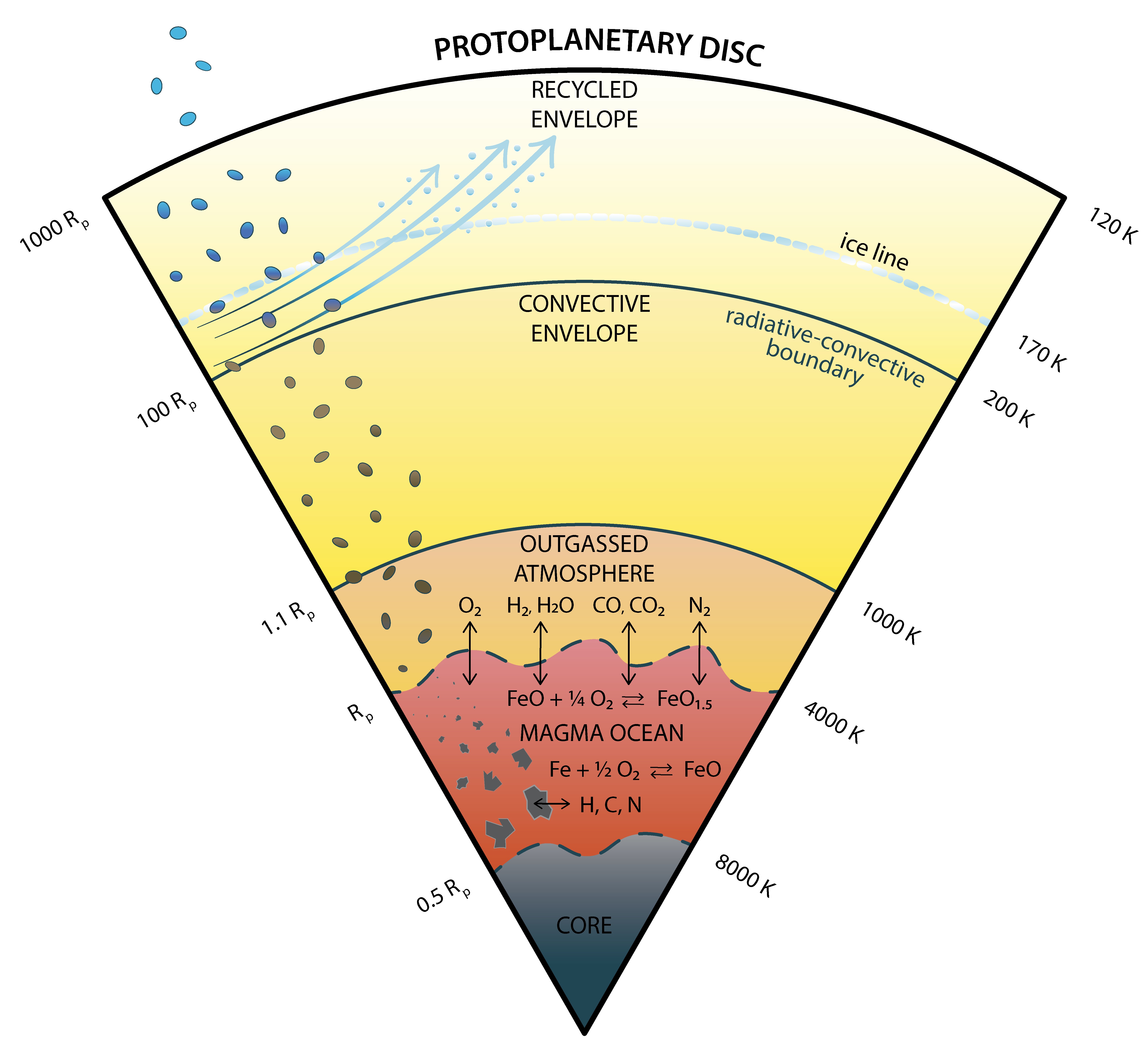
Figure 1: Overview of the core, mantle, atmosphere and envelope of a rocky planet growing by rapid pebble accretion. The protoplanetary disc flows penetrate through the recycled part of the envelope, carrying along water vapour released at the ice line at $T\approx 170$ K back to the protoplanetary disc. The radiative-convective boundary at $T\approx 200$ K marks the transition to a bound, convective envelope. The desiccated pebbles sediment through the convective gas down to the outgassed atmosphere. The atmosphere is in vapour equilibrium with the silicate magma ocean and pebbles therefore survive until they plunge into the magma ocean. Here the metal separates from the silicates and metal blobs coalesce and sediment to the core. There is an equilibrium between the concentration of volatiles H, C and N in the magma ocean and the outgassed atmosphere. The speciation of the volatiles in the atmosphere depends on the oxygen fugacity of the magma ocean, which is set by the iron-wüstite buffer Fe + (1/2) O₂ $\leftrightharpoons$ FeO. The lower regions of the magma ocean undergoes additional oxidation by the process FeO + (1/4) O₂ $\leftrightharpoons$ FeO_1.5. Finally, the volatiles H, C, and N are all siderophile and partition primarily into metallic melt over silicate melt. This results in a core that holds the main reservoirs of H and C, while N has so low solubility in magma that the atmosphere is the dominant reservoir of nitrogen.

2 ADAP code modules on atmospheric escape

The interior structure and outgassing modules of the ADAP code are described in Paper I and Paper II. Here we describe our approach to atmospheric mass loss after the dissipation of the protoplanetary disc.

2.1 Atmospheric escape

We follow Erkaev et al. (2007) and Salz et al. (2016) and define the mass loss rate of the atmosphere as

$$\dot{M}=\frac{3\beta^{2}\eta F_{\rm XUV}}{4KG\rho_{\rm pla}}\,.$$ (1)

Here $\beta=R_{\rm XUV}/R_{\rm pla}$ parameterizes the effective capture radius of XUV photons $R_{\rm XUV}$ relative to the planetary radius $R_{\rm pla}$, $\eta$ is the efficiency of mass loss relative to the energy-limited expression (defined as $\eta=1$), $F_{\rm XUV}$ is the energy flux in the XUV range by the young Sun, $K$ is a parameter of the order of unity that parameterizes the effect of the stellar gravity on the planetary loss rate and $\rho_{\rm pla}$ is the internal mass density of the planet.

We assume for simplicity that the mass loss occurs only through direct acceleration of H atoms and the associated drag by the escaping H on the heavier species C, O, and N. The intense radiation environment at the base of the thermosphere is assumed to dissociate all molecules into their constituent atoms (Erkaev et al., 2014). We define from equation (1) an equivalent number loss rate of hydrogen atoms with of mass $\mu_{\rm H}$ as

$$\dot{N}_{\rm H}^{\star}=\frac{3\beta^{2}\eta F_{\rm XUV}}{4KG\rho_{\rm pla}\mu_{\rm H}}X_{\rm H}\,.$$ (2)

Here $N_{i}$ is the total number of atoms of species $i$ (where $i$ denotes the atomic species H, C, O, and N), $X_{i}=n_{i}/n$ is the mixing ratio of species $i$ in the thermosphere, with $n=\sum_{i}n_{i}$ denoting the sum of the number density of all species $n_{i}$, taking into account that the water mixing ratio may fall with height due to water cloud condensation (see Paper II). The multiplication by the hydrogen mixing ratio $X_{\rm H}$ into the number loss rate in equation (2) reflect the energy lost to heating of species other than H. We thus assume that the absorption of XUV radiation (a) has a similar cross section for H, C, O, and N atoms and (b) only leads to escape of H while the heavier species remain bound even after absorption of an XUV photon. These assumptions allow us to make relatively simple calculations of the escape of primordial atmosphere dominated by hydrogen.

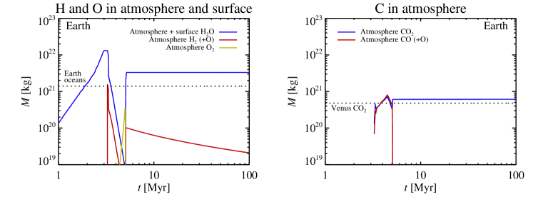
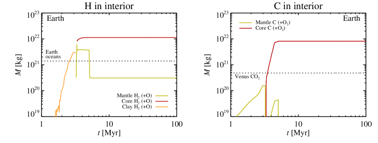
Figure 2: The evolution of H-bearing (left panels, including O₂) and C-bearing volatiles (right panels) in the atmosphere and surface (top panels) and interior (bottom panels) of our Earth analogue. Hydrogen resides initially in a massive surface layer of ice and water and an interior layer of clay. The onset of the run-away greenhouse effect after 3.5 Myr heats the surface to form a global magma ocean. The water dissolves in the magma and partitions within the magma ocean strongly into the metal melt. The core of Earth incorporates after the termination of accretion more than 90% of the total hydrogen and carbon budgets. The oxygen fugacity of the magma ocean rises with increasing temperature and hence O₂ becomes the dominant molecule in the atmosphere at the end of the accretion stage; this oxygen is nevertheless dissolved back into the magma ocean as it cools. The terrestrial magma ocean expels approximately one modern ocean mass of water after crystallization of the magma. The oxidized atmosphere of Earth avoids any extensive mass loss by XUV irradiation and maintains an atmosphere consisting mainly of CO₂ with a mass similar to modern Venus’ atmosphere.

All the atmospheric components escape together, driven by drag from the hydrogen atoms but maintaining their initial mixing ratio. We assume that the mixing ratio in the thermosphere is the same as in the bulk atmosphere, neglecting any scale-height differences due to the mean molecular weight. This gives a number loss rate of the mixed species as

$$\dot{N}=\frac{\dot{N}_{\rm H}^{\star}}{X_{\rm H}+X_{\rm C}(\mu_{\rm C}/\mu_{\rm H})+X_{\rm O}(\mu_{\rm O}/\mu_{\rm H})+X_{\rm N}(\mu_{\rm N}/\mu_{\rm H})}\,.$$ (3)

Here $\mu_{i}$ is the atomic weight of species $i$. The individual number loss rates can then be written as

$$\dot{N}_{i}=X_{i}\dot{N}\,,$$ (4)

which maintains the mixing ratio $\dot{N}_{i}/\dot{N}=N_{i}/N_{\rm all}$ for H, C, O, and N. We furthermore need to ensure that the drag from the escaping H atoms is sufficient to accelerate the heavier species to the escape speed. This is seen by calculating the escape parameter

$$\varPhi_{i}=\frac{\dot{N}_{\rm H}k_{\rm B}T_{\rm photo}}{3\pi GM_{\rm pla}\mu_{i}b_{{\rm H},i}}\,.$$ (5)

Here $T_{\rm photo}$ is the temperature at the photosphere and $b_{{\rm H},i}$ is the binary diffusion coefficient of species $i$ dragged by H (Zahnle & Kasting, 1986; Erkaev et al., 2014). We then set $\dot{N}_{i}=0$ when $\varPhi_{i}<(\mu_{i}-\mu_{\rm H})/\mu_{i}$, assuming that the energy transferred from H to the heavier species in that case goes to heating but does not lead to escape. This way the H escape flux drives the escape of the heavier species only when the flux is high, while the heavy species (C, N, O) eventually decouple from the H drag for lower flux values. The H flux decreases both because the H mixing ratio of the atmosphere decreases and because the XUV luminosity of the young Sun falls with time.

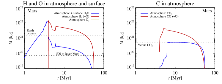
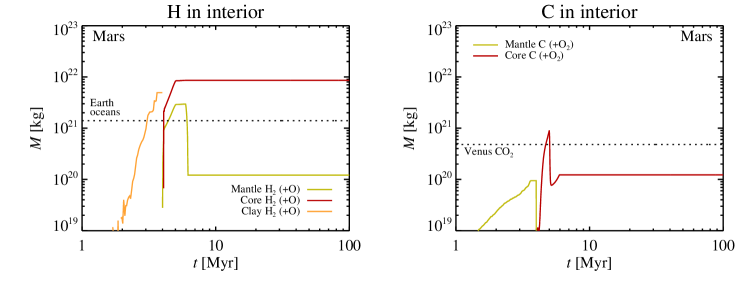
Figure 3: The evolution of the H-bearing and C-bearing volatiles in our Mars analogue. The smaller martian core can only hold 50% of the water, resulting in the outgassing of a massive H₂-dominated atmosphere (we show for H₂ its equivalent water mass). The dominant H₂ component of Mars’ atmosphere undergoes hydrodynamical escape within 70 Myr and drags along with it the entire atmospheric CO, CO₂ and H₂O contents.

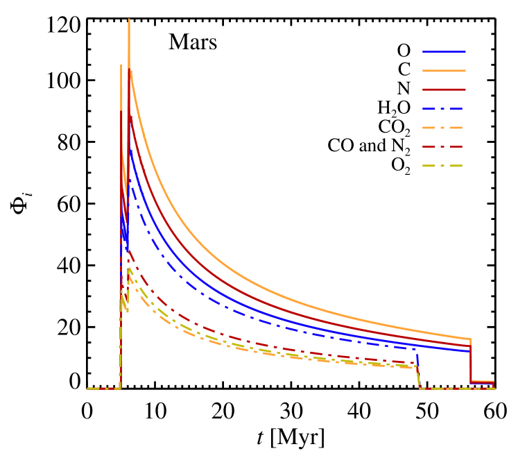
Figure 4: The escape parameter $\varPhi_{i}$ as a function of time for our Mars analogue. We show results both for our standard assumption that molecules are dissociated into O, C, and N in the thermosphere (full lines) as well as for an alternative model where the molecules are assumed to remain intact (dash-dotted lines). We bundle CO and N₂ together in the plot, due to their similarity in both binary diffusion coefficient (Zahnle & Kasting, 1986) and molecular weight; this gives a similar escape parameter. The escape flux of hydrogen is in all cases high enough to drag along all heavier species ($\varPhi_{i}\gg 1$) until all the hydrogen has been depleted.

To test the sensitivity of our results to the assumption that all molecules are atomic at the thermosphere, we implemented an additional model where H is atomic but H₂O, CO₂, CO, N₂, and O₂ remain molecular. These heavier molecules are harder to lift by the escaping hydrogen atoms. We use here equations (3), (4) and (5) but with molecular binary diffusion coefficients $b_{{\rm H},i}$ for the relevant molecules provided in Zahnle & Kasting (1986). Due to the lack of data for molecular oxygen dragged by atomic H in Zahnle & Kasting (1986), we set by analogy $\varPhi_{\rm O_{2}}=\varPhi_{\rm N_{2}}$. We ignore the sedimentation of the heavier species from the thermosphere, since this has only little effect on the escape rates for our relevant values of $\varPhi_{i}\gg 1$ (Zahnle & Kasting, 1986; Zahnle et al., 1990; Erkaev et al., 2014). We refer to Hunten et al. (1987) and Wordsworth et al. (2018) for detailed analysis of the hydrodynamical escape problem and the conditions for successful drag of heavier species.

For the capture radius $\beta$ and the efficiency relative to energy-limited escape $\eta$ in equation (2), we follow the parameterizations fitted to computer simulations by Salz et al. (2016). The efficiency flattens out to a relatively constant value of around 30% for the low-mass planets considered here, while the capture radius increases with decreasing planetary mass as the gravitational acceleration decreases, increasing the scale-height of the atmosphere. For the first 100 Myr of solar evolution, we read off a fit to the data of Tu et al. (2015) of

$$L_{\rm XUV}=L_{1}(t/{\rm Myr})^{-0.75}\,,$$ (6)

with the luminosity at 1 Myr set for simplicity to a nominal value of $L_{1}=10^{24}\,{\rm J\,s^{-1}}$. The XUV flux is then calculated as $F_{\rm XUV}=L_{\rm XUV}/(4\pi r^{2})$ where $r$ is the distance from the star. The decrease of the luminosity with time becomes steeper after a few hundred 100 Myr of stellar rotation evolution, but we do not include these later stages of atmospheric evolution here.

2.2 Core-powered mass loss

Core-powered mass loss has been proposed as another important loss mechanism affecting planetary hydrogen/helium envelopes (Ginzburg et al., 2016, 2018), complementing the loss by XUV photoevaporation. The mass loss rate of the envelope is here given by the thermal flux of gas at the sonic radius $R_{\rm s}=GM_{\rm pla}/(2c_{\rm s}^{2})$ where the envelope ceases to be bound in the absence of an external pressure (Gupta & Schlichting, 2019). The sound speed at the photosphere, $c_{\rm s}$, is set by the effective cooling temperature of the planet. The mass loss rate for the core-powered mass loss mechanism is proportional to the density at the photosphere of the envelope, and this density is in turn proportional to the total mass of the envelope. Our planets have hydrogen/helium envelopes of relatively low masses ($M_{\rm env}\sim 10^{19}\,{\rm kg}$ for Earth $M_{\rm env}\sim 10^{17}\,{\rm kg}$ for Mars, see Paper II). The mass loss rates for the low-mass envelope cases considered here are thus dominated by XUV photoevaporation, since that loss rate is independent of the mass of the envelope and hence very effective on low-mass envelopes. We therefore do not include core-powered mass loss in the calculations.

2.3 Stellar irradiation

The radiative heating of the young planets by the Sun also becomes relevant once the protoplanetary disc has vanished. We assume that the stellar luminosity was 70% of the luminosity of the modern Sun and that the planets had the same albedo as modern-day Venus ($A=0.77$). This high value of the albedo combined with the faint, young Sun implies that both Earth and Venus condense their water vapour atmospheres into oceans. Complex atmospheric circulation models and realistic albedo values are needed to understand whether Venus started off with a run-away greenhouse atmosphere or whether surface oceans condensed out on early Venus (Way et al., 2016; Turbet et al., 2021). We illustrate the effect of the surface albedo by performing an additional numerical experiment with a lower value of the planetary surface albedo, $A=0.3$ representing a relatively cloud-free planet such as modern Earth.

3 Partitioning and loss of H-bearing and C-bearing molecules

We ran simulations for model analogues of Earth, Mars, and Venus using simple exponential growth rates as in Paper II. Mars and Venus were evolved to their current masses, while Earth grew to only $0.6\,M_{\rm E}$ within the adopted 5 Myr lifetime of the protoplanetary disc. This is because of the later collision with the additional planet Theia, assumed here to have a mass of $0.4\,M_{\rm E}$, to form the Moon. In Paper II we demonstrated that Theia must have had a mass of at least $0.3\,M_{\rm E}$ to satisfy the low ¹⁸²W abundance in the Earth’s mantle after the collision.

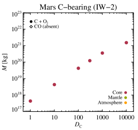
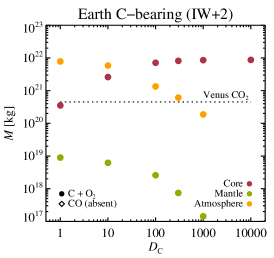
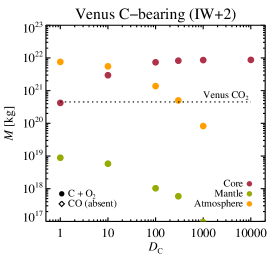
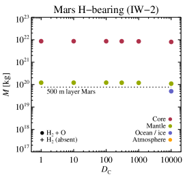
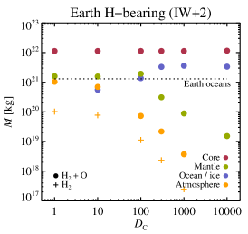
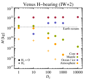
Figure 5: The distribution of C-bearing (top) and H-bearing (bottom) volatiles between core, mantle, ocean, and atmosphere after 100 Myr of atmospheric evolution, as a function of the carbon partition coefficient $D_{\rm C}$ between metal and silicate melt. Mars loses its entire atmospheric reservoirs due to atmospheric escape for all values of $D_{\rm C}$. The martian mantle nevertheless maintains a significant amount of H₂ that can be released as water and reduced H₂ by later volcanism or impacts and drive short-lived warming events. Some ice condenses out at the surface of Mars for the highest value of $D_{\rm C}$ where most C is in the core and the atmosphere thus very cold. Earth and Venus experience only little atmospheric escape. Their atmospheric contents of CO₂ match the current atmospheric contents of Venus best for a partition coefficient around $D_{\rm C}=300$. Higher partition coefficients bury too much carbon in the core. A partition coefficient around our nominal choice of $D_{\rm C}=300$ also gives a good match of the outgassed water mass of Earth and Venus to the modern Earth ocean mass.

3.1 Choice of partition coefficients and oxidation state

We are particularly interested in understanding the effect of the partition coefficients of H, C, and N between metal melt and silicate melt, $D=C_{\rm met}/C_{\rm sil}$ with $C_{\rm met}$ denoting the equilibrium mass concentration in metal melt and $C_{\rm sil}$ the equilibrium mass concentration in silicate melt. The measured partition coefficients intrinsically depend on both temperature and pressure; additionally they come with large experimental uncertainties and interdependencies between the dissolved species. We therefore vary the partition coefficients around a set of chosen nominal values. We choose nominal values $D_{\rm H}=5$ (Li et al., 2020), $D_{\rm C}=300$ (Fischer et al., 2020) and $D_{\rm N}=10$ (Grewal et al., 2019a) and examine how the results depend on varying the partition coefficients around those values, with $D_{\rm H}$ in the range from 1 to 10, $D_{\rm C}$ in the range from 1 to 10,000 and $D_{\rm N}$ in the range from 1 to 100. We study a very large variation in the carbon partition coefficient since the partition coefficient has been determined experimentally to display a parabolic dependence on the pressure, with high partition coefficients at both low ($\sim$Mars) and high ($\sim$Earth) magma ocean pressures (Fischer et al., 2020).

The outgassing of O₂ from the magma ocean is key to determining the speciation between H₂/H₂O and CO/CO₂ in the outgassed atmosphere. We choose nominal oxidation states of the mantles of Earth and Venus as IW+2 (where IW denotes the iron-wüstite buffer Fe + (1/2) O₂ $\leftrightharpoons$ FeO, see Paper II), while we assume a much more reduced mantle two log-units below the buffer (IW-2) for Mars (Armstrong et al., 2019; Ortenzi et al., 2020). The loss of O by atmospheric escape should lead to a reduction of the oxygen fugacity. We proposed in Paper I that this reduction could be significant for a small body like Vesta. However, planetary-mass bodies have enormous oxygen reservoirs bound as FeO in their mantles. We calculate that Mars would have to lose of the order of 10 Earth oceans and Earth and Venus would have to lose of order the order of 100 Earth oceans to affect the total oxygen budget of mantle plus atmosphere. We therefore do not change the oxygen fugacity due to atmospheric loss.

3.2 Evolution of the outgassed atmosphere

In Figures 2 and 3 we show the evolution of H-bearing, C-bearing species as well as O₂ for our Earth and Mars analogues. During the earliest accretion stages, hydrogen resides mainly as water in a massive surface ocean and bound as OH in the clay layer below. As the water ocean undergoes a run-away greenhouse effect after 3.5–4 Myr, the water enters first the atmosphere as steam and is subsequently dissolved in the newly formed magma ocean. For Earth, the magma ocean transfers more than 90% of the water into the core-forming metal. Approximately one Earth ocean mass of water is outgassed following the termination of accretion after 5 Myr, leaving only small amounts of water in the mantle (Elkins-Tanton, 2008).

The magma ocean has a low ability to dissolve CO₂, so the carbon in our Earth analogue distributes mainly between the core (holding 90% of the carbon) and the atmosphere. The outgassed CO₂ forms a dense greenhouse atmosphere with a temperature of $T_{\rm surf}=500$ K. This is cool enough to condense a global water ocean which would subsequently re-bury CO₂ in the mantle after precipitation of dissolved CO₂ to the ocean floor as carbonates (Sleep & Zahnle, 2001; Taylor et al., 2018).

Mars initially undergoes a similar evolution to Earth, but its lower mantle oxidation state results in the outgassing of large amounts of H₂. The hydrodynamical escape of H drives a catastrophic atmospheric mass loss during the first 70 Myr of stellar activity evolution, leading to the escape of the entire atmosphere (Erkaev et al., 2014). The mantle of Mars stores $(2-3)\times 10^{16}\,{\rm kg}$ of CO₂, which is approximately equal to the modern CO₂ reservoirs of Mars. The martian mantle also stores H₂ equivalent of approximately 0.1 terrestrial ocean mass if oxidized. However, this hydrogen storage would be degassed as 10% H₂O and 90% H₂ in volcanism and impacts, due to the low oxygen fugacity of the martian mantle. In this picture of early loss of the primordial CO₂ atmosphere followed by a gradual resupply from the mantle, the inferred flow of liquid water on Mars likely took place during short-lived heating events caused by impacts that released large amounts of gases such as H₂ that acted as temporary thermal blanketing (Wordsworth et al., 2017; Deng et al., 2020b).

3.3 The efficiency of atmospheric escape

In Figure 4 we show the escape parameter $\varPhi_{i}$ of atoms and molecules dragged by atomic hydrogen (defined in equation 5). The hydrogen flux is unable to lift the heavier atoms and molecules when $\varPhi_{i}<(\mu_{i}-\mu_{\rm H})/\mu_{i}\approx 1$, where $\mu_{i}$ is the mass of atom or molecule $i$. The escape parameter is much larger than unity for both atoms and molecules in our Mars analogue and therefore the atmosphere undergoes total escape without leaving heavier species behind. This happens irrespective of whether or not we assume all molecules to be dissociated to atoms in the thermosphere.

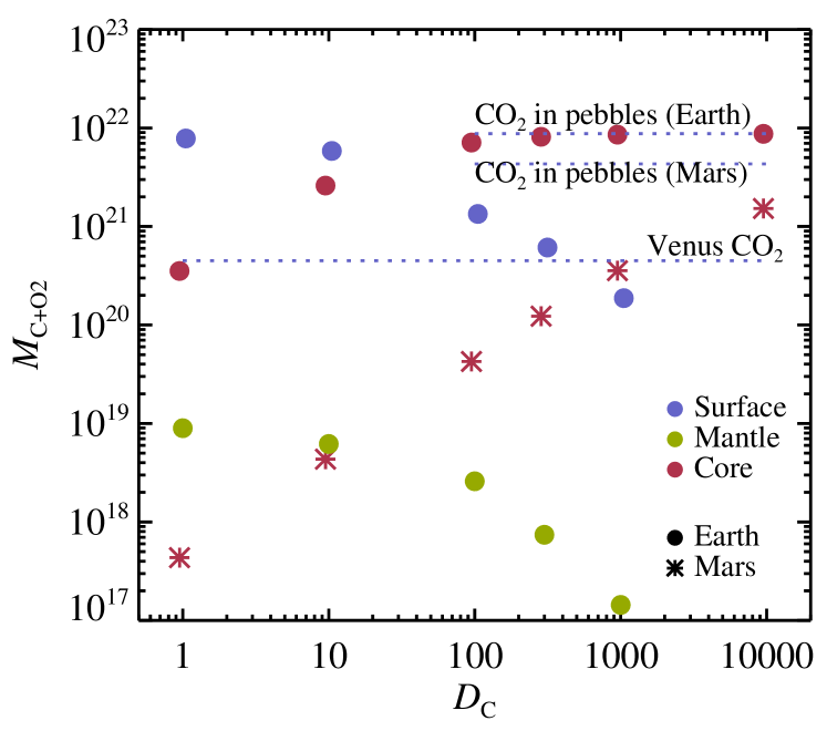
Figure 6: The mass of CO₂ in the surface, mantle and core reservoirs after 100 Myr of evolution for Earth (filled circles) and Mars (asterisks) as a function of the partition coefficient of carbon between metal melt and silicate melt. The measurement is given for C + O₂ to reflect the CO₂ equivalent mass of the dissolved C in the core and the mantle. We mark the accreted CO₂ for Earth and Mars as well as the modern CO₂ reservoir in Venus’ atmosphere. Lowering the partition coefficient leads to a decreased carbon storage in the core and more outgassing to the surface. The mantle holds negligible carbon in all cases. The escape of the reduced martian atmosphere removes any outgassed CO or CO₂ reservoirs from Mars. The symbols are displaced slightly horizontally to better distinguish them.

The partial pressure of oxygen is fixed in our model by the assumption that the magma ocean works as an oxygen buffer with a fixed fugacity (Ortenzi et al., 2020). Hirschmann (2020) proposed that the outgassing and escape of H₂ (or correspondingly, the ingassing of O₂ from thermal destruction of H₂O in the atmosphere) could increase the oxidation state in the martian mantle and lead to outgassing of more oxidized species. This view nevertheless does not take into account that the oxygen released in the atmosphere could instead undergo atmospheric escape together with the hydrogen and hence maintain the mean planetary oxidation state if the escape occurs at a relative rate of ${\rm O/H}=0.5$.

3.4 Varying the partition coefficient of carbon

The adopted value of the partition coefficient of carbon between metal and silicate melt, $D_{\rm C}$, has key influence on the outgassed atmosphere. In Figure 5 we show the reservoirs of water CO₂, H₂, and CO in the core, mantle, ocean, and atmosphere after 100 Myr of atmospheric evolution. The carbon reservoirs on Earth and Mars are compared directly in Figure 6 as a function of the partition coefficient $D_{\rm C}$. We show the results for a range of $D_{\rm C}$ values between 1 and 10,000. The atmosphere of Mars is not much affected by this choice, since the atmosphere is lost under all circumstances. The amount of carbon trapped in the core becomes significant above $D_{\rm C}=300$, but 90% of the carbon is lost to atmospheric escape even for large values of $D_{\rm C}$. The cores of Earth and Venus, in contrast, hold much larger reservoirs of C, unless the $D_{\rm C}$ value is 10 or lower. Very low values of $D_{\rm C}$ result in an extremely massive CO₂ atmosphere of more than 10 times the modern Venus atmospheric mass.

The surface water reservoir of Mars (in the form of a global ice layer) is only significant in the bottom-left panel of Figure 5 for the highest value of $D_{\rm C}=10000$ where the blue dot approaches 500 metres of surface ice. This assumption stores the most C in the core and therefore the atmosphere is colder. Some water is thus maintained during atmospheric escape as the thinning atmosphere cools to condense out a global ice layer of approximately 500 m depth. For lower values of $D_{\rm C}$, the ice reservoir on Mars becomes absent. There is nevertheless significant water stored in mantle minerals for all values of the carbon partition coefficient (green dots).

Venus and Earth instead hold approximately 2.5 modern ocean masses of water in their atmospheres and ocean. The balance shifts from ocean to atmosphere below $D_{\rm C}=100$, as the greenhouse effect from the CO₂ is then substantial enough to keep the temperature above the critical point of water. Hence, Earth and Venus evolve very similarly. However, this is under the luminosity of the faint young Sun, set here to 70% of the modern value. Venus is therefore expected to undergo a run-away greenhouse effect involving dissociation and loss of water as the Sun increased its luminosity on the main sequence.

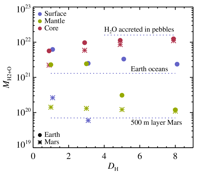
Figure 7: The mass of water in the surface (condensed and vapour), mantle, and core reservoirs after 100 Myr of evolution for Earth (filled circles) and Mars (asterisks) as a function of the partition coefficient of water between metal melt and silicate melt. The measurement is given for H₂+O to reflect the H₂O equivalent mass of the dissolved H in the core and the mantle. The best match to the surface water reservoir of Earth is found for high values of $D_{\rm H}=5$ and $D_{\rm H}=8$. Mars, on the other hand, loses all its surface water unless $D_{\rm H}=3$ or less. The core reservoir mass falls with decreasing $D_{\rm H}$, particularly for Mars that has a smaller core than Earth. This hydrogen was outgassed as H₂ from the martian mantle and subsequently lost to hydrodynamical escape. The mantles of Earth and Mars store significant H₂ reservoirs that can later be outgassed as H₂ and H₂O in volcanism and after impacts. The symbols are displaced slightly horizontally to better distinguish them.

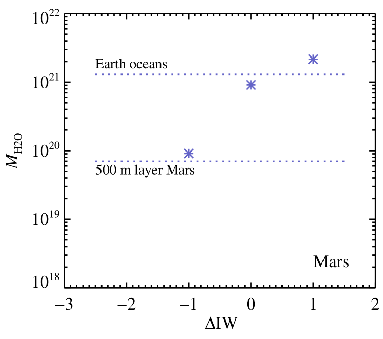
Figure 8: The mass of water in the surface reservoir of Mars (condensed and vapour) as a function of the oxidation state of the mantle relative to the iron-wüstite buffer (IW), with higher values of $\Delta{\rm IW}$ indicating increasing partial pressure of oxygen in the atmosphere. The top line marks the modern Earth ocean mass, while the bottom line marks a 500 metre water layer on Mars. For the nominal value of $\Delta{\rm IW}-2$, Mars loses its entire surface and atmosphere water reservoir, but the water amount increases rapidly from IW-1 and upwards.

3.5 Varying the partition coefficient of water

The partition coefficient of water between metal melt and silicate melt also affects strongly the distribution of water between the atmosphere, mantle, and core. In Figure 7 we show the mass of water in the three reservoirs for Earth and Mars, as a function of $D_{\rm H}$ that we vary between 1 and 8, bracketing the range of values reported in Li et al. (2020). As $D_{\rm H}$ is lowered, progressively more water moves from the core to the atmosphere. The best consistency with the Earth’s surface reservoir is found for high values of $D_{\rm H}=5$ (2.6 oceans) and $D_{\rm H}=8$ (1.8 oceans). Mars only maintains surface water for $D_{\rm H}\leq 3$, which is much lower than the nominal value for the partition coefficient.

3.6 Varying the oxidation state of Mars

We assumed a nominal oxidation state of the mantle of Mars of ${\rm IW}-2$, which is valid for a completely open contact between the metal in the core and the FeO in the mantle (Frost et al., 2008) with no further self-oxidation taking place at high pressures (Armstrong et al., 2019). This value clearly leads to complete loss of the water from the martian surface reservoir. To understand how the results depend on the value of $\Delta{\rm IW}$, we ran simulations for oxidation states between ${\rm IW}-2$ and ${\rm IW}+1$. The results are shown in Figure 8. The surface water reservoir increases steeply when going from very low oxidation states towards ${\rm IW}+0$. Beyond ${\rm IW}+1$, most of the hydrogen is outgassed from the magma ocean as H₂O and the total amount of water in the surface reservoir saturates. The best match to Mars’ estimated primordial surface water reservoir comes at an oxygen fugacity slightly above ${\rm IW}-1$. This increase over the nominal value could indicate that Mars’ magma ocean FeO was slightly decoupled from the core material when the atmosphere was outgassed.

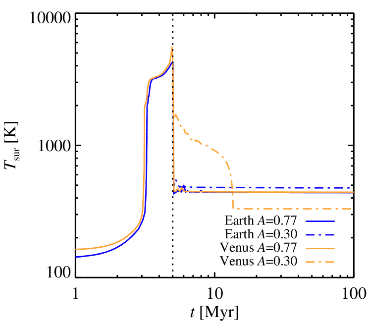
Figure 9: The surface temperature as a function of time for our Earth and Venus analogues evolved for two different values of the planetary albedo. The Earth analogue experiences only a slight delay in the cooling when considering the lower albedo value, while the cooling of Venus surface is delayed for more than 10 Myr. The prolonged state of high surface temperature leads to efficient escape of dissociated H₂O and CO₂; thus the surface temperature of Venus eventually lands at a lower value than Earth’s.

3.7 Varying the planetary albedo

Finally, we compare the surface temperature evolution of Earth and Venus for two values of the planetary albedo: $A=0.77$ (our nominal choice, representing modern Venus with reflective clouds) and $A=0.3$ (which represents better a relatively cloud-free planet such as modern Earth). The results are shown in Figure 9. The high surface temperatures experienced during the accretion phase are caused by the blanketing effect of CO₂ and H₂O. Earth cools down very quickly after the termination of the accretion at $t=5\,{\rm Myr}$. Venus, in contrast, evolves very differently for the low-albedo case. Here the cooling of the surface is delayed by more than 10 Myr. The vicinity of Venus to the Sun in combination with low albedo maintains a surface temperature of around 1,000 K. Interestingly, the surface temperature eventually drops as the water vapour in the hot photosphere is easily driven away by the XUV radiation from the young star. This drags along with it significant amounts of CO₂ as well, which leads to a colder planetary surface than Earth. We nevertheless consider the high-albedo case more realistic, since this reflects better the reflection of solar radiation by clouds in high-temperature atmospheres and is based on modern Venus as a template.

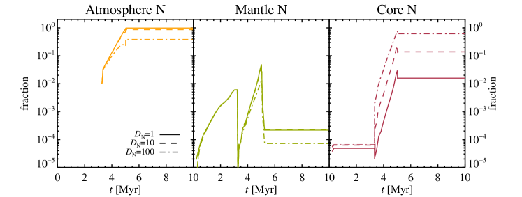
Figure 10: Evolution of the mass fraction in the N₂ reservoirs atmosphere, mantle and core for different values of the metal-silicate partition coefficient $D_{\rm N}$ in our Earth analogue. We set here the total nitrogen mass to an arbitrary value of $3.8\times 10^{18}\,{\rm kg}$, similar to the modern terrestrial atmosphere reservoir. Since N₂ in our model does not affect the thermodynamics or mass of the planet, this choice is arbitrary. We show the results for three values of the metal-silicate partition coefficient, $D_{\rm N}=1,10,100$. However, the partitioning between core and mantle has to compete also with the outgassing of N₂ to the atmosphere. This means that even $D_{\rm N}=100$ leads only to approximately equal masses of nitrogen in the atmosphere and in the core. Hence it is hard to store significant amounts of N in the core of Earth.

4 Nitrogen partitioning

The distribution of nitrogen between the atmosphere and the core is of particular interest for understanding the source material of Earth. The atmosphere of Earth contains approximately 0.5 ppm of nitrogen, normalized by the full mass of the planet. This is in stark contrast to several hundred ppm found in enstatite chondrites and even higher values in the carbonaceous chondrites (Grewal et al., 2019a). Grewal et al. (2021) proposed that large amounts of N are sequestrated in the core of Earth. Transport of nitrogen from the mantle to the core is expected due to the strong partitioning of N into the metal melt over the silicate melt. The partition coefficient could be as high as $D_{\rm N}=10$ or even $D_{\rm N}=100$ for relatively oxidized magma compositions (Grewal et al., 2019a). However, the transport of N from mantle to core has to compete with strong tendency for outgassing of nitrogen into the atmosphere (Speelmanns et al., 2019).

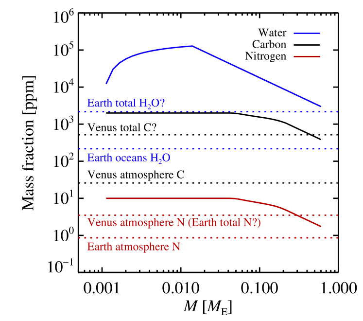
Figure 11: The mass fraction of water, carbon and nitrogen for the Earth analogue model of Johansen et al. (2021) as a function of the accreted mass. The dotted lines shows constraints from the volatile reservoirs of Earth and Venus, together with estimates of the total water and carbon including the core. The volatiles are accreted with pebbles mainly in the early stages of planet formation where the envelope temperature is low. We find overall good matches to the water and carbon contents of Earth and Venus, as in Johansen et al. (2021). The pebble accretion model also gives a good match to the nitrogen reservoirs in the atmospheres of Earth and Venus. In contrast, the enstatite chondrites, often considered a possible source material of Earth (Dauphas, 2017), have N contents above 100 ppm and hence provide a poor match to the nitrogen budget of Earth (Grewal et al., 2019a).

4.1 Modelling nitrogen partitioning

In addressing the nitrogen problem, we first calculate the relative distribution of nitrogen between atmosphere, mantle, and core. We assume here that nitrogen constitutes a constant fraction of the accreted material at an (arbitrary) total amount corresponding to the atmospheric inventory of the modern Earth. In Figure 10 we show the fraction of N₂ in the different mass reservoirs for our Earth analogue as a function of time for partition coefficients $D_{\rm N}=1,10,100$. For low values of $D_{\rm N}$, the majority of the nitrogen ends in the atmosphere, with only a small amount distributed to the core. Even for $D_{\rm N}=100$ the core and atmosphere inventories only become about equal; this is due to the low dissolution of N in the magma melt. Hence even large values of $D_{\rm N}$ do not lead to a substantially higher core reservoir than mantle reservoir. This implies then that no chondrites class, except perhaps the ordinary chondrites, provides the right amount of nitrogen to be reservoirs for Earth formation. This leaves differentiated bodies that experienced extensive N outgassing and loss as a possible source planetesimals for Earth formation (Grewal et al., 2019b). Samples of planetesimals that formed early enough to melt (e.g. Vesta meteorites, ureilites, angrites) nevertheless have isotopic compositions of lithophile elements such as Cr and Ca that disagree with Earth (Schiller et al., 2018; Zhu et al., 2021). In contrast, if Earth formed mainly by accreting pebbles, then the nitrogen depletion can be well understood from the same thermal processing that filtered away water and carbon.

In Johansen et al. (2021) we calculated the final mass fraction of water and carbon for Earth, using source material where the early accretion phase consists of 35% mass of water and 3,000 ppm mass of carbon, while the late-accreted outer Solar System material carries 5% carbon (Alexander et al., 1998). This material is then processed in the hydrostatic hydrogen envelope of the planet, with the accreted water fraction dropping to zero when the envelope acquires a temperature above 160 K and carbon sublimated and pyrolized in successive steps from 325 K to 1,100 K (Gail & Trieloff, 2017). Here we extend this analysis to nitrogen. We assume that the N contents of the NC reservoir (characteristic of inner Solar System material) is 10 ppm, while the N contents of the CC reservoir (characteristic of outer Solar System material) is 500 ppm, the majority of this nitrogen residing in the organics (Alexander et al., 1998). Nitrogen is then released as volatile species between 325 K and 425 K, following the sublimation and pyrolysis of the carbon in the organics (Nakano et al., 2003; Gail & Trieloff, 2017).

4.2 Nitrogen in core, mantle, and atmosphere

In Figure 11 we show the mass fraction (in ppm) of water, carbon, and nitrogen for our Earth analogue as a function of its accreted mass. We overplot the water ocean reservoir on Earth, the carbon atmospheric reservoir of Venus and the nitrogen atmospheric reservoirs of Venus and Earth. Mysen (2019) estimated the mantle reservoir of N on Earth to be twice the atmospheric value. This way the total N contents of Earth correspond well to the total mass of atmospheric N on Venus. The release of the bulk N contents of Venus to its atmosphere could be due to oxidation of the mantle by oxygen left over from the loss of water in the upper atmosphere (Wordsworth, 2016b). Since significant amounts of water and carbon may be stored in the cores of Venus and Earth, we also plot estimated values of these total reservoirs.

Figure 11 confirms that the water and carbon reservoirs of Earth fit well with the pebble accretion model. The nitrogen gives an equally good fit. The low nitrogen contents of the NC reservoir (at 10 ppm) combined with thermal processing in the envelope at elevated planetary masses gives a final mass fraction of nitrogen of around 2 ppm. This is in stark contrast to the nitrogen contents of the enstatite chondrites, often considered the source material of Earth (Dauphas, 2017). At several 100 ppm of nitrogen, the enstatite chondrites could at most have provided a percent of the final masses of Earth and Venus. The nitrogen isotopes of iron meteorites are divided in a neutron-poor NC component and a neutron-rich CC component (Grewal et al., 2021). The isotopic composition of the Earth’s nitrogen could in the pebble accretion picture reflect the accretion of neutron-poor nitrogen carried by pebbles of inner Solar System composition combined with the late accretion of a few mass percent of nitrogen-rich planetesimals from the outer Solar System (Marty, 2012; Bekaert et al., 2020). Scaling the planetesimal source material instead to ordinary chondrites, using the abundances from Bekaert et al. (2020), yields instead 5–10% contribution from accretion of chondrites to Earth. Such planetesimal contribution levels (a few percent CC or up to 10% OC) would also deliver reasonable fits to the noble gas abundance of our planet (Marty, 2012).

5 Summary of pebble accretion model for terrestrial planet formation

In our three papers on the anatomy of rocky planets forming by pebble accretion, we have explored a novel model for the formation of terrestrial planets where the solid mass of the planets as well as the volatiles are delivered mainly via pebbles (see our overview of the model in Figure 1). This idea is attractive to explore for three major reasons: (i) observations of protoplanetary discs reveal large populations of mm-sized pebbles – planetary building blocks in the pebble accretion model – around young stars (Zhu et al., 2019), (ii) measurements of the isotopic composition of Earth and the known meteorite classes show that our planet incorporated a large fraction ($\sim$40%) mass with the composition of material from the outer Solar System that was likely delivered to our planet via drifting pebbles (Schiller et al., 2018), and (iii) while the pebble accretion was developed in order to explain the rapid formation of the cores of gas giants in the outer Solar System (Ormel & Klahr, 2010; Lambrechts & Johansen, 2012), the large flux of pebbles drifting through the terrestrial planet region must by extension have played a role in the assembly of terrestrial planets as well (Johansen et al., 2021).

In Paper I we identified the core mass fraction and FeO mantle fraction of terrestrial planets and planetesimals as a direct consequence of the formation of the terrestrial planets by pebble accretion exterior of the water ice line. Water is accreted as ice as long as the envelope is not yet hot enough to sublimate the ice into water vapour that is recycled with hydrodynamical flows back to the protoplanetary disc. Upon melting by the accretion heat, the water oxidizes metallic iron to form magnetite. This oxidized iron in turn becomes unavailable to contribute to the core. We could therefore show that the increasing core mass fraction and decreasing FeO mantle fraction of the Vesta, Mars, Earth triplet is consistent with iron oxidation by early exposure to liquid water. This in turn implies that the core mass fraction of terrestrial planets is a monotonously decreasing function of the planetary mass, with the extrapolated expectation that massive super-Earths should have a very high core mass fraction if they formed by pebble accretion near the water ice line.

The differentiation of such rapidly formed planets occurs via the continuous release of accretion energy rather than via giant impacts that melt the mantle, as we demonstrated in Paper II. The retention of the pebble accretion heat requires a thermally blanketing atmosphere and here the accreted volatiles play an important role in outgassing an early atmosphere of H₂O and CO₂ that traps the accretion heat. The core of Earth thus forms within the lifetime of the protoplanetary disc and this would seem at first glance to be in conflict with the Hf-W dating of core formation, which yields ages in excess of 35 Myr (Kleine & Walker, 2017). However, we demonstrated in Paper II that a moon-forming giant impact occurring after 40–60 Myr resets the Hf-W clock and makes the Earth appear younger than its actual bulk core formation time of only 5 Myr after the formation of the Sun.

Thermal processing of pebbles in the envelope of the growing planets is a key difference between the pebble accretion model and the traditional view that volatiles are delivered via planetesimal impacts. Particularly, the terrestrial planets can grow exterior of the water ice line without accreting excessive amounts of volatiles (Johansen et al., 2021). Nitrogen appears to be a decisive volatile in this connection. In solid substances, this atom resides mainly in organic molecules in the inner regions of the protoplanetary disc and is hence released successively as the organics sublimate and pyrolyse at increasing temperatures. This way we demonstrated in Paper III that the 10 ppm concentration of nitrogen typical of ordinary chondrite meteorites that formed in the asteroid belt region is reduced to a few ppm (parts-per-million) by thermal processing, in agreement with the nitrogen reservoirs residing in the atmospheres of Earth and Venus. This contrasts strongly to the several hundred ppm of refractory nitrogen found in enstatite chondrites (Grewal et al., 2019a), often considered a potential source material for Earth (Dauphas, 2017).

We demonstrated here in Paper III that the surface water reservoir of Earth as well as the CO₂ contents of Venus’ atmosphere are reproduced well in the pebble accretion model using nominal values for the partition coefficients of these volatiles between metal melt and silicate melt. Preventing complete loss of the martian surface water requires a slight increase in the oxygen fugacity of the mantle over the nominal value of ${\rm IW}-2$, indicating perhaps a gradual decoupling of the magma ocean from the metal in the core. The mantles of our model Venus, Earth and Mars also store significant hydrogen that can later be outgassed as H₂ and H₂O, depending on the evolution of the mantle oxygen fugacity with time. The cores of the terrestrial planets hold under all circumstances large reservoirs of H and C that were trapped in the descending metal droplets during the core-formation stage.

In summary, we believe that we have demonstrated that our pebble accretion model for terrestrial planet formation displays several key consistencies with the observed properties of the terrestrial planets in the Solar System. This in turn implies that these well-studied terrestrial planets can be used as benchmark cases for the testing of a self-consistent planet formation model that can subsequently be applied to predict the properties of the interiors and atmospheres of extrasolar rocky planets as well as the early conditions on the surface when prebiotic chemistry strives towards ever increasing complexity.