Anatomy of rocky planets formed by rapid pebble accretion
II. Differentiation by accretion energy and thermal blanketing

We explore the heating and differentiation of rocky planets that grow by rapid pebble accretion. Our terrestrial planets grow outside of the ice line and initially accrete 28% water ice by mass. The accretion of water stops after the protoplanet reaches a mass of $0.01\,M_{\rm E}$ where the gas envelope becomes hot enough to sublimate the ice and transport the vapour back to the protoplanetary disc by recycling flows. The energy released by the decay of ²⁶Al melts the accreted ice to form clay (phyllosilicates), oxidized iron (FeO), and a water surface layer with ten times the mass of Earth’s modern oceans. The ocean–atmosphere system undergoes a run-away greenhouse effect after the effective accretion temperature crosses a threshold of around 300 K. The run-away greenhouse process vaporizes the water layer, thereby trapping the accretion heat and heating the surface to more than 6,000 K. This causes the upper part of the mantle to melt and form a global magma ocean. Metal melt separates from silicate melt and sediments towards the bottom of the magma ocean; the gravitational energy released by the sedimentation leads to positive feedback where the beginning differentiation of the planet causes the whole mantle to melt and differentiate. All rocky planets thus naturally experience a magma ocean stage. We demonstrate that Earth’s small excess of ¹⁸²W (the decay product of ¹⁸²Hf) relative to the chondrites is consistent with such rapid core formation within 5 Myr followed by equilibration of the W reservoir in Earth’s mantle with ¹⁸²W-poor material from the core of a planetary-mass impactor, provided that the equilibration degree is at least 25%-50%, depending on the initial Hf/W ratio. The planetary collision must have occurred at least 35 Myr after the main accretion phase of the terrestrial planets.

1 Introduction

Observations of young stars reveal that they are surrounded by very massive protoplanetary discs of gas and dust, with a typical early-stage protoplanetary disc containing several hundred Earth masses of solids in the form of millimetre-sized pebbles (Tychoniec et al., 2018; Carrasco-González et al., 2019). These pebbles play an important role in the theory of planetesimal formation, as the streaming instability (Johansen et al., 2007; Bai & Stone, 2010), likely in combination with weak pressure bumps that form in the turbulent gas (Stoll & Kley, 2016; Manger & Klahr, 2018; Yang et al., 2018; Schäfer et al., 2020), can concentrate pebbles into dense filaments that undergo contraction and gravitational collapse to form planetesimals with a characteristic size of 100 km (Johansen et al., 2015; Simon et al., 2016; Nesvorný et al., 2019).

Pebbles can also drive planetary growth beyond the planetesimal stage. The characteristic pebble size of 0.1–1 millimetre, inferred from observations of protoplanetary discs (Zhu et al., 2019; Liu, 2019), is in the right size range for frictional energy dissipation to be significant during the scattering by a growing protoplanet, which leads to capture and accretion of the pebble by the protoplanet. This pebble accretion process has growth rates that are significantly enhanced relative to the accretion rate of large planetesimals (Johansen & Lacerda, 2010; Ormel & Klahr, 2010; Lambrechts & Johansen, 2012). High pebble accretion rates are likely necessary to form planets akin to the gas giants and ice giants in the Solar System where planetesimal accretion fails to form cores within the lifetime of the protoplanetary disc (Bitsch et al., 2015; Johansen & Bitsch, 2019; Tanaka & Tsukamoto, 2019).

The inner regions of the protoplanetary disc – where the terrestrial planets and super-Earths form – are also traversed by the large population of drifting pebbles. The traditional terrestrial planet formation theory was nevertheless developed around a combination of planetesimal accretion and giant impacts between the growing protoplanets (Kokubo & Ida, 1998) with water delivery by rare impacts of icy planetesimals (Raymond et al., 2004). The low value of the excess of ¹⁸²W relative to the non-radiogenic isotopes ¹⁸³W and ¹⁸⁴W in Earth’s mantle is interpreted as evidence that Earth formed relatively slowly by accumulation of planetesimals and smaller protoplanets. The isotope ¹⁸²W is created by the decay of ¹⁸²Hf with a half life of approximately 8.9 Myr (Kleine & Walker, 2017). Since Hf is lithophile and W is moderately siderophile, a low excess of ¹⁸²W indicates protracted core formation. However, it is not clear whether the Hf-W age of Earth is a measure of the true accretion time or whether it is set mainly by a later moon-forming giant impact. Such a giant impact may have been the result of an instability among a terrestrial planet system that originally contained more planets (Canup, 2012; Quarles & Lissauer, 2015; Johansen et al., 2021). The main core formation stage of Earth could therefore have lasted closer to 10 Myr, followed by a moon-forming giant impact occurring more than 50 Myr later (Yin et al., 2002; Yu & Jacobsen, 2011).

Rapid pebble accretion must consequently be explored as a serious candidate for the formation mechanism of terrestrial planets, both around the Sun and around other stars. Lambrechts et al. (2019) demonstrated how the radial mass flux of pebbles determines whether protoplanets in the inner regions of the protoplanetary disc grow to Mars-sized protoplanets or continue to form migrating chains of super-Earths. Johansen et al. (2021) instead explored intermediate pebble fluxes and found that the masses, orbits and volatile budgets of the terrestrial planets in the Solar System (except Mercury) are consistent with starting as protoplanets at the primordial ice line and then growing and migrating to their current masses and orbits.

All four terrestrial planets in the Solar System are differentiated into a metallic core dominated by iron and a silicate mantle where iron is only present in the form of oxidized FeO (see Carlson et al., 2014; Trønnes et al., 2019, for recent reviews). This widespread differentiation implies that melting of the terrestrial planets was a natural consequence of their accretion and early evolution – and that all terrestrial planets go through a magma ocean stage where the mantle was partially or wholly molten (Elkins-Tanton, 2012; Schaefer & Elkins-Tanton, 2018). Impacts are traditionally invoked to explain the formation of such magma oceans (Matsui & Abe, 1986a, b; Righter & Drake, 1999; Wade & Wood, 2005; Rubie et al., 2015a). The necessity for widespread magma oceans also implies that the primordial atmospheres of the terrestrial planets were outgassed from the global magma ocean as it recrystallized and expelled its incompatible volatiles. The composition of the primordial atmospheres of terrestrial planets was thus controlled by the overall budgets of the main volatiles H, C, and N combined with the oxygen released by the dominant Fe-O-FeO reactions occurring in the magma ocean (Schaefer & Fegley, 2010; Ortenzi et al., 2020). The crystallization partitioned a small fraction of the volatiles into solid crystals in the mantle that can be compared to current constraints on carbon and hydrogen reservoirs in the terrestrial mantle (Elkins-Tanton, 2008).

In Paper I of this series, we demonstrated how planetesimals forming outside the ice line melt and desiccate through heat release by the decay of ²⁶Al. Energy from the decay of ²⁶Al runs out after a few half-lives ($t_{1/2}=0.7\,{\rm Myr}$). We continue to explore here in Paper II the interior evolution of planets that form by rapid pebble accretion. We add mass accretion to the model and follow the heating and differentiation of the interior of the growing planet, the outgassing of an early atmosphere that acts as thermal blanketing, the emergence of a magma ocean and the differentiation of the planet into a metal core and a silicate mantle. We show that rapid accretion by pebble accretion combined with thermal blanketing from an outgassed atmosphere leads to widespread melting of planets as they grow beyond approximately 1% of an Earth mass. This way pebble accretion naturally explains the emergence of the magma oceans that are needed to understand differentiation and atmospheric outgassing. We furthermore demonstrate that the relatively small excess of ¹⁸²W in Earth, when compared to very early formed bodies such as Vesta, is consistent with a main accretion phase lasting only 5 Myr followed by a moon-forming impact after 40–60 Myr that exchanged enough tungsten isotopes between the core of the impactor and the mantle of Earth to lower the ¹⁸²W excess to its observed value.

The paper is organized as follows. In Section 2 we describe the modules of the ADAP code related to partitioning of volatiles (H, C, O, and N) between the core, mantle and atmosphere. In Section 3 we present the results of running the ADAP code for the full accretion of a terrestrial planet. We focus particularly on comparing the heating and differentiation of an Earth analogue and a Mars analogue. In Section 4 we turn to calculating the evolution of the Hf and W contents of the mantle and core of Earth before and after the moon-forming impact. We show that the formation of Earth by rapid pebble accretion is consistent with the low excess of ¹⁸²W in the mantle of Earth for significant impactor masses (higher than $0.2\,M_{\rm E}$) and high core-mantle equilibration. We summarize our results in Section 5. Appendix A describes our algorithm for calculating the temperature and pressure structure of the outgassed atmosphere and the envelope of gas attracted from the protoplanetary disc.

2 ADAP code modules on volatile partitioning

We describe here the aspects of the ADAP code related to distributing volatiles between the core, mantle and atmosphere as well as the structure and cooling rate of the outgassed atmosphere and accreted gas envelope. The interior heating and composition evolution model of ADAP is described in Paper I. The atmospheric composition is simplified to consist of the molecules H₂O, CO₂, H₂, CO, O₂ and N₂. These molecules are assumed to be stored as H₂O, CO₂ and N₂ within the mantle and core of the growing planet. The oxygen fugacity of the magma ocean sets the speciation of H (H₂O or H₂) and C (CO₂ and CO) as they outgas to the atmosphere. We include additionally the evaporation under very hot conditions of non-volatile silicates from the magma ocean.

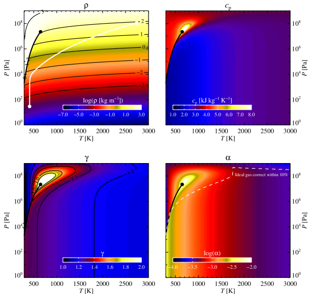
Figure 1: Equation of state of water based on the IAPWS prescription (http://www.iapws.org/). The top left plot shows the density of the water as a function of temperature and pressure. The thick black line indicates the saturated vapour pressure and the black dot the critical point beyond which the distinction between liquid and vapour vanishes. The white line shows the structure of the atmosphere of our Earth analogue at the beginning of the differentiation phase ($t=3.5$ Myr). The top right plot shows the heat capacity at constant pressure and the bottom left the ratio of the specific heats, $\gamma=c_{\rm p}/c_{\rm v}$. Finally, the bottom right plot shows the thermal expansion coefficient $\alpha$, which is needed to calculate the adiabatic lapse rate of the planetary atmosphere. For an ideal gas law, $\alpha=(1/V)(\partial V/\partial T)_{P}=1/T$. The dashed line indicates where the ideal gas law expression is correct within 10% in the calculation of $\alpha$.

The terrestrial planets grow massive enough inside the protoplanetary disc to attract a significant hydrostatic envelope of hydrogen and helium gas (Stökl et al., 2016; Johansen et al., 2021). This envelope adds additional thermal blanketing to the surface and therefore must be included in the calculations.

2.1 Atmosphere structure

The surface pressure at the bottom of the atmosphere is calculated from

$$P_{\rm sur}=\frac{gM_{\rm atm}}{4\pi R^{2}}+P_{\rm env}\,.$$ (1)

Here $g$ is the gravitational acceleration at the surface, $M_{\rm atm}$ is the sum of the masses of the atmospheric components, $R$ is the planetary radius (i.e. the distance from its centre to the solid or liquid surface, not including the atmosphere) and $P_{\rm env}$ is the pressure at the bottom of the hydrostatic gas envelope attracted from the protoplanetary disc. The outgassed atmosphere transitions continuously to the attracted envelope in both temperature and density at the pressure level $P=P_{\rm env}$. We assume that the transition in mean molecular weight at the atmosphere-envelope transition will create a narrow radiative zone at the transition, preventing mixing of atmospheric constituents into the envelope. The complete structure of the atmosphere-envelope system is thus given uniquely by the outwards-transported luminosity, the mass of the atmosphere and the boundary conditions of the envelope towards the protoplanetary disc. We assume further that the atmospheric scale-height is so low that $g$ is constant and attains the value at the planetary surface throughout the extent of the atmosphere $z$ (measured from the surface).

The full scheme for finding the atmosphere-envelope structure and luminosity for a given surface temperature is given in Appendix A. We use here an analytical solution for the envelope structure based on the analysis presented in Piso & Youdin (2014). The outgassed atmosphere can not in general be assumed to follow an ideal gas law, particularly when water vapour is under pressure and temperature beyond the critical point. We therefore perform a full numerical integration of the atmosphere from the surface to the atmosphere-envelope transition.

The vertical temperature gradient of the atmosphere $\varGamma=-\partial T/\partial z$ is constructed to follow either a dry adiabat,

$$\varGamma=\frac{\alpha Tg}{c_{\rm p}}\,,$$ (2)

or a more complex moist adiabat (including cloud particles) when the water vapour in the atmosphere is saturated (Leconte et al., 2013). Here $\alpha$ is the thermal expansion coefficient, $T$ is the temperature and $c_{\rm p}$ is the specific heat at constant pressure. Knowing the temperature lapse rate, the pressure and density follow from hydrostatic equilibrium and an equation of state.

The equation of states for CO₂, H₂, CO, O₂ and N₂ are all assumed to follow the ideal gas law; this yields a simple measure of the thermal expansion coefficient as $\alpha=1/T$. The specific heat capacities at constant pressure of these gases are calculated from polynomial fits provided at the NIST Chemistry WebBook (https://webbook.nist.gov/chemistry/). Since water undergoes transitions both from vapour to liquid and from ideal gas to supercritical gas phase, we adopted a parameterized gas law for water based on the IAPWS prescription. We show our calculation of the equation of state of water in Figure 1. We create a look up table of the water density, specific heats and thermal expansion coefficient at the set up of a simulation and use this table for rapid, interpolated look-ups during runtime. Any water amount in excess of the saturated vapour pressure at a given height over the surface is converted to cloud particles with zero contribution to pressure, but including the contribution of the liquid or frozen droplets to both density and heat capacity.

2.2 Luminosity carried through atmosphere and envelope

We calculate the luminosity transported from the planetary surface through the atmosphere and envelope as

$$L_{\rm atm}=4\pi R^{2}\sigma_{\rm SB}(T_{\rm sur}^{4}-T_{\rm atm}^{4})\,,$$ (3)

where $\sigma_{\rm SB}$ is the Stefan-Boltzmann constant, $T_{\rm sur}$ is the temperature of the planetary surface, and $T_{\rm atm}$ is the temperature at the bottom of the atmosphere. We iterate on this luminosity until the boundary conditions of the protoplanetary disc at the Hill sphere are fulfilled (see Appendix A). This approach will nevertheless lead to very high surface temperatures (up to 10,000 K or more). This is not realistic, since the critical point of SiO is approximately 6,600 K (Xiao & Stixrude, 2018), above which the magma ocean has no distinct liquid and vapour phases. Pebbles would thus not reach the surface and the accretion energy would be released where the pebbles are dissolved higher up the atmosphere; this will prevent burial of the accretion heat and thus reduce the temperature at the surface. We therefore distribute part of the pebble accretion heat at the bottom of the envelope, rather than in the surface layer, when the temperature of the lower atmosphere is above a threshold value of $T_{\rm atm,max}=3{,}000\,{\rm K}$. We do not release any silicate vapour in the hydrostatic envelope above the atmosphere (Brouwers et al., 2018); this assumption is valid for the relatively modest temperatures reached in the base of the envelope (see Figure 8).

The fraction of accretion energy dissipated in the bottom of the envelope is set to

$$f_{\rm acc,env}=\tanh[(T/T_{\rm atm,max})^{10}]\,.$$ (4)

This ensures a transition width of a few hundred K from 100% energy release in the surface layer ($f_{\rm acc,env}=0$) to 100% energy release at the bottom of the envelope ($f_{\rm acc,env}=1$). The heating of the surface is thus reduced to $L_{\rm sur}=(1-f_{\rm acc,env})L_{\rm acc}$ and the bottom of the envelope carries the total luminosity

$$L_{\rm env}=L_{\rm atm}+f_{\rm acc,env}L_{\rm acc}\,.$$ (5)

After the dissipation of the protoplanetary disc, the external boundary condition no matter bears physical meaning. Instead, the luminosity known from equation (3) will then define the temperature $T_{2/3}$ at optical depth $\tau=2/3$ through

$$L=4\pi R_{\rm pho}^{2}\sigma_{\rm SB}T_{2/3}^{4}\,,$$ (6)

with $R_{\rm pho}$ denoting the photosphere radius. In Appendix A we describe how this is calculated from the knowledge of the envelope opacity and the luminosity.

In the absence of a gas envelope, for example after its removal by XUV radiation, the photospheric temperature level $T_{2/3}$ is reached in the outgassed atmosphere. In that case we integrate

$${\rm d}\tau=\kappa(P)\rho{\rm d}z$$ (7)

from $\tau=0$ to $\tau=2/3$. We use an opacity law $\kappa=\kappa_{0}(P/P_{0})^{q}$ that is proportional to the local pressure $P$ ($q=1$, see Badescu, 2010), with $P_{0}=1.013\times 10^{5}$ Pa and $\kappa_{0}=1.0\,{\rm m^{2}\,kg^{-1}}$ for water (Matsui & Abe, 1986a; Nakajima et al., 1992; Koll & Cronin, 2019) and $\kappa_{0}=0.0005\,{\rm m^{2}\,kg^{-1}}$ for CO₂. The other atmospheric components are assumed to carry insignificant opacities. Elkins-Tanton (2008) discusses whether a low value (our nominal choice) or a high value for the opacity of CO₂ is most realistic. We demonstrate in Figure 2 the photospheric temperature of a Venus analogue planet with a pure CO₂ atmosphere and a range of surface pressures and surface temperatures. We also vary the opacity law from linear with $P$ (the nominal choice) to constant. We find the best value for the surface temperature of Venus to be represented by $\kappa_{0}=0.0005\,{\rm m^{2}\,kg^{-1}}$ for CO₂ with a linear opacity law. This choice of a low CO₂ opacity agrees with the CO₂ atmosphere models of Wordsworth (2015) and Salvador et al. (2017).

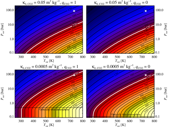
Figure 2: Photospheric temperature of a Venus analogue (in terms of mass and radius), for a range of surface temperatures ($x$-axis) and surface pressure ($y$-axis). The atmospheric composition is assumed to be 100% CO₂. The top plots utilize a high CO₂ opacity, while the bottom plots are calculated using our nominal value that is 100 times lower (see discussion in Elkins-Tanton, 2008). The left plots use the nominal linear dependence of the opacity on the pressure, while the right plots show the difference when using a pressure-independent opacity instead. Our atmosphere model becomes invalid below the horizontal black line, which indicates the transition to an optically thin atmosphere. The effective temperature of Venus (220 K, when taking into accounts its relatively high current opacity) is indicated with a thick line and the temperature and surface CO₂ pressure with an asterisk. We choose therefore the low opacity value and linear pressure dependence to best reproduce the atmosphere of Venus in our calculations.

The water opacity influences the transition from stable atmosphere to run-away greenhouse effect. Ingersoll (1969) demonstrated that a pure water atmosphere in equilibrium with a surface ocean will obtain a maximum cooling rate at an effective temperature of around 300 K, beyond which any increase in the surface temperature will not lead to additional cooling (see also Hamano et al., 2013; Kopparapu et al., 2013). We test the run-away greenhouse effect for an Earth analogue in Figure 3. Using the opacity model of Matsui & Abe (1986a), with $\kappa_{0}=0.01\,{\rm m^{2}\,kg^{-1}}$ at one atmosphere pressure and linear pressure dependence, the transition to run-away greenhouse effect happens at a surface temperature of around 320 K. Goldblatt et al. (2013) demonstrated using frequency-dependent radiative transfer models that the transition happens at an outgoing flux of 282 ${\rm W}\,{\rm m}^{-2}$. On the other hand, Leconte et al. (2013) found a limiting flux of 375 ${\rm W}\,{\rm m}^{-2}$. We match this range of values best with a much higher water opacity level with $\kappa_{0}=1.0\,{\rm m^{2}\,kg^{-1}}$ and therefore adopt this (with linear pressure dependence) as our nominal value. We experiment in Figure 7 with lower values of the water opacity to assess how this affects the differentiation of the planet.

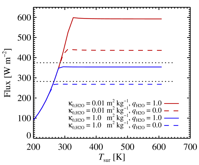
Figure 3: The thermal flux escaping the top of a pure water atmosphere for a range of surface temperatures. The run-away greenhouse effect manifests itself as a plateau in the outgoing flux: there is no stable thermal equilibrium when the external or internal heating is higher than this critical flux $F_{\rm crit}$. We mark the Goldblatt et al. (2013) result of a full frequency-dependent radiative transfer 1-D model ($F_{\rm crit}=282\,{\rm W\,m^{-2}}$) and the Leconte et al. (2013) result of a 3-D climate model ($F_{\rm crit}=375\,{\rm W\,m^{-2}}$) with dotted lines. The grey opacity parametrization of Matsui & Abe (1986a), with $\kappa_{0}=0.01\,{\rm m^{2}\,kg^{-1}}$ and linear pressure dependence (full red line), results in a too high critical flux value. We find a better match when adopting a two orders of magnitude higher opacity, $\kappa_{0}=1.0\,{\rm m^{2}\,kg^{-1}}$.

2.3 Hydrogen opacity

We assume that the H₂ molecule carries zero opacity in our calculations. At high densities of CO₂ and H₂, collision-induced absorption can raise the opacity of the H₂ molecule to significant values (Karman et al., 2019). We therefore performed a numerical experiment with an H₂ opacity equal to the (high) H₂O opacity. We found the H₂ opacity to have very little effect on the mass onset for differentiation (see effect of water opacity in Figure 7). This is likely due both to the high water opacity, which makes other opacity sources insignificant, and to the fact that the flux threshold for the run-away greenhouse effect depends only weakly on the opacity (see Figure 3).

2.4 Atmospheric escae

We describe our energy-limited approach to remove the outgassed atmosphere and the envelope by XUV irradiation in Paper III.

2.5 Water evaporation

We outgas a water vapour atmosphere from surficial and underground water (evaporation) or ice (sublimation) by calculating the saturated vapour pressure of water, $P_{\rm sat}$, at the equilibrium temperature $T_{\rm equ}$ using the IAPWS equation of state. In equilibrium, the water mixing ratio $X_{\rm H_{2}O}$ at the surface must fulfil

$$P_{\rm sat}=X_{\rm H_{2}O}P_{\rm sur}\,.$$ (8)

Using equation (1) and an expression for the mixing ratio, the right hand side can further be expanded as

$$P_{\rm sat}=\frac{M_{\rm sat}/\mu_{\rm H_{2}O}}{\sum_{i}M_{i}/\mu_{i}}\left(\frac{g\sum_{i}M_{i}}{4\pi R^{2}}+P_{\rm env}\right)\,.$$ (9)

Here $M_{i}$ is the mass of the $i$th atmospheric component, with $M_{i}=M_{\rm sat}$ for water. We solve Equation (9) for the saturated water mass $M_{\rm sat}$ by transforming the equation to a second order polynomial.

When the surface layer is ice or water, then we evaporate or condense $f=0.1$ times the difference between the current atmospheric water mass and the saturated water mass. However, we limit the outgassed mass to be $f$ times the total water mass remnant in the planet. This ensures that the atmosphere and the surface reach equilibrium within a few ten time-steps. We have compared a simulation with $f=0.001$ to the nominal simulation with $f=0.1$ and found nearly identical results; hence the vapour equilibrium is obtained on a short enough time-scale that disequilibrium effects do not affect the results.

We check also whether the local pressure is higher than the saturated vapour pressure below the surface. Deep boiling of water occurs whenever $P(r)<P_{\rm sat}(r)$. This is particularly true when the water temperature is above the critical temperature in which the liquid phase ceases to exist and the saturated vapour pressure is formally infinite. We assume the deep boiling leads to vapour bubble formation and outgassing at the local surface. In that case, we require that the partial pressure of water in the atmosphere to equal the deep boiling saturated pressure. This typically leads to outgassing of the entire water contents of the protoplanet.

2.6 Evaporation of silicates

At surface temperatures above approximately 2,000 K, the silicate magma ocean equilibrates with a significant vapour pressure in the atmosphere. The vapour pressure over the magma ocean consists of a mixture of molecules such as Mg, SiO, O and O₂ (Schaefer & Fegley, 2004). We follow the approach of Misener & Schlichting (2022) and define a temperature-dependent effective silicate vapour pressure over the magma ocean, with a single mean molecular weight. We choose SiO as the representative molecule of the silicate vapour; we refer to Misener & Schlichting (2022) for a discussion of using a slightly lighter value to reflect the mixture of species in the vapour. We set the critical temperature to 6,600 K (Xiao & Stixrude, 2018), above which we freeze the saturation pressure at the critical pressure level of $P_{\rm crit}=1.9\times 10^{4}\,{\rm bar}$. We use an ideal gas equation of state for the SiO in the atmosphere; this is a valid approximation because any SiO pressure in excess of the critical pressure is not allowed to leave the magma ocean. We include formation of SiO clouds in cooler layers above the surface, using a scheme similar to water clouds. We ignore any latent heat release in SiO cloud formation.

As discussed above, we limit the surface temperature to approximately 3,000 K to reflect pebble destruction in the atmosphere. We motivate this choice here, because at such temperatures silicates will dominate the composition of the atmosphere. Silicate clouds will thus form high up in the atmosphere and we assume that pebbles colliding with these clouds will be destroyed and hence release their accretion energy at the base of the envelope rather than in the magma ocean.

2.7 Carbon and nitrogen release

We treat carbon and nitrogen as trace species that do not contribute to the bulk planetary mass (although both species add mass and pressure to the atmosphere and carbon carries also atmospheric opacity). We set the carbon contents of the accreted material to 2,000 ppm up to a maximum carbon amount of $4\times 10^{-4}$ $M_{\rm E}$. This follows the model of volatile accretion by pebble snow from Johansen et al. (2021) where the carbon in organics is sublimated between 325 K and 425 K and the remaining carbon in graphite burns at a temperature of 1,100 K (Gail & Trieloff, 2017) and subsequently diffuses back to the protoplanetary disc within ultravolatile molecules such as CH₄ and CO. We assume that the carbon forms carbonates in the mantle after the melting of the ice and that these carbonates decompose at $T_{\rm dec}=1000$ K, releasing carbon into the mantle as CO₂. For the nitrogen, we assume that it resides mainly in the organics and is released, together with the carbon, successively between 325 K and 425 K (Nakano et al., 2003; Gail & Trieloff, 2017). We release the nitrogen into the mantle at $T_{\rm dec}=1000$ K, similarly to the carbon, and limit the total nitrogen amount to the current atmosphere of Earth, $M_{\rm N_{2}}=3.87\times 10^{18}$ kg. Since atmospheric nitrogen does not contribute to the heating of the surface, the total amount of nitrogen in the model is arbitrary and we are mainly interested in how the nitrogen partitions between core, mantle and atmosphere – this partitioning is discussed further in Paper III.

2.8 Water dissolution in magma

For the dissolution of water in magma we calculate first the total mass of molten silicates $M_{\rm mag}$. We then calculate the equilibrium mass fraction of water in the melt from Matsui & Abe (1986a, b),

$$X_{\rm wat}=2.08\times 10^{-6}(P_{\rm H_{2}O}/{\rm Pa})^{0.54}\,.$$ (10)

This equilibrium describes the reaction between O^2- ions in the magma melt and gaseous H₂O to form dissolved OH^- radicals (Iacono-Marziano et al., 2012; Ortenzi et al., 2020). The reaction of two OH^- radicals to reform H₂O explains the square-root like pressure-dependence in equation (10). We calculate $X_{\rm wat}$ from the water surface pressure $P_{\rm sur,H_{2}O}$ and then we transfer 0.1 times the difference between the equilibrium value of the water mass in the silicates and the actual value between the atmosphere and the silicates. The magma ocean is assumed to equilibrate with the atmosphere when the magma is present at higher levels than 80% of the current protoplanet radius. We define here magma as those spherical shells that have a melt fraction higher than $\varPhi_{\rm melt}=0.5$.

2.9 CO₂ and N₂ dissolution in magma

For partitioning of CO₂ between magma and atmosphere, we use the equilibrium atmospheric partial pressure from Papale (1997) and Hirschmann (2012),

$$X_{{\rm CO}_{2}}=4.4\times 10^{-12}(P_{\rm CO_{2}}/{\rm Pa})\,.$$ (11)

This equilibrium describes the reaction between O^2- ions in the magma melt and gaseous CO₂ to form dissolved carbonate CO${}_{3}^{2-}$ (Iacono-Marziano et al., 2012; Ortenzi et al., 2020). The CO₂ solubility changes with pressure and temperature at depth of the magma ocean, first increasing for the terrestrial magma ocean down to a few hundred kilometers and then falling until diamond condenses out at depths below 500 km (Hirschmann, 2012; Armstrong et al., 2019), corresponding to a pressure between 15 and 20 GPa. The concentration of carbon in the magma ocean is nevertheless set by the equilibrium concentration of CO₂ at the surface interface, as this value is maintained throughout the magma ocean by convection. Lower solubility at depth implies that the molecular storage of carbon changes but the concentration does not change as long as the diamond crystals do not grow to large enough sizes to sediment. We note that Elkins-Tanton (2008) seem to use a much higher value for the solubility of carbon in magma that is close to the solubility value for water (their equations 3 and 4).

For N₂, we follow Sossi et al. (2020) and set the equilibrium concentration in the magma ocean according to

$$X_{{\rm N}_{2}}=6.11\times 10^{-13}(P_{\rm N_{2}}/{\rm Pa})\,.$$ (12)

This expression is valid for relatively oxidized conditions, while extremely reduced conditions not encountered during the differentiation of Earth and Mars (but maybe relevant for Mercury) are characterized by very high chemical dissolution values (Libourel et al., 2003). We refer to Lichtenberg et al. (2021) for a recent overview of the different dissolution laws and their applicability ranges.

2.10 Hydrogen, carbon and nitrogen in the core

We consider the core and the mantle to be continuously connected through a partition coefficient $D=C_{\rm cor}/C_{\rm man}$ where $C_{\rm cor}$ is the concentration of the species in the core and $C_{\rm man}$ is the concentration of the species in the magma mantle. This yields an equilibrium mantle concentration of

$$C_{\rm man}=\frac{M_{\rm vol}}{DM_{\rm cor}+M_{\rm man}}\,,$$ (13)

where $M_{\rm vol}$, $M_{\rm man}$ and $M_{\rm cor}$ are the instantaneous masses of the volatile species under consideration, the mantle and the core, respectively. Volatiles may in reality not be able to partition continuously between metal and silicates subsequent to their initial transport to the core. Assuming therefore that volatiles partition only between metal and silicates during their descent through the mantle yields the mantle equilibrium concentration

$$\dot{C}_{\rm man} = \frac{{\rm d}}{{\rm d}t}\left(\frac{M_{\rm vol,man}}{M_{\rm man}}\right)$$ (14)

$$= \frac{\dot{M}_{\rm vol,man}}{M_{\rm man}}-\frac{M_{\rm vol,man}}{M_{\rm man}^{2}}\dot{M}_{\rm man}$$

$$= \frac{\dot{M}_{\rm vol}}{M_{\rm man}}-D\frac{M_{\rm vol,man}}{M_{\rm man}}\frac{\dot{M}_{\rm cor}}{M_{\rm man}}-\frac{M_{\rm vol,man}}{M_{\rm man}^{2}}\dot{M}_{\rm man}$$

$$= \frac{\dot{M}_{\rm vol}}{M_{\rm man}}-DC_{\rm man}\frac{\dot{M}_{\rm cor}}{M_{\rm man}}-C_{\rm man}\frac{\dot{M}_{\rm man}}{M_{\rm man}}\,.$$

This differential equation has an equilibrium solution, with $\dot{C}_{\rm man}=0$, given by the mantle concentration

$$C_{\rm man}=\frac{\dot{M}_{\rm vol}}{D\dot{M}_{\rm cor}+\dot{M}_{\rm man}}\,.$$ (15)

When $D$ is assumed to be a constant that does not depend on temperature and pressure and all mass accretion rates are proportional to the instantaneous mass (so that $\dot{M}_{i}=(M_{i}/M)\dot{M}$ for all components), then equation (15) transforms to the same as expression as when assuming continuous partitioning between core and mantle (equation 13). Since we consider constant $D$ in the simulations in order to probe the range of possible values for the partition coefficients, we apply equation 13 in each time-step to determine the equilibrium concentrations of volatiles in the mantle and the core.

Hydrogen, carbon and nitrogen are all siderophile elements with an affinity to enter metallic melt over silicate melt. For hydrogen, we base our partition coefficients between metal and silicates on Kuramoto & Matsui (1996) and Li et al. (2020) and take a base value of $D_{\rm H}=5$. For carbon, Fischer et al. (2020) provided fits for $D_{\rm C}$ over a range of pressure and temperatures. Since the partition coefficient of carbon depends so strongly on the planetary mass, we experiment with a range of values of $D_{\rm C}$ around a base value of 300. Nitrogen does not affect the evolution of our planets and is used mainly as a tracer for comparing observed atmospheres with our model atmospheres. Nitrogen partition coefficients additionally show strong dependencies on the oxygen fugacity of the mantle (Grewal et al., 2019). We therefore experiment with partition coefficients for N between $D_{\rm N}=1$ and $D_{\rm N}=100$ to bracket the range of realistic values, with a base value of $D_{\rm N}=10$.

The core is assumed to equilibrate with the magma ocean when the lowest molten molten mantle is less than 10% of the protoplanet radius away from the core-mantle boundary.

2.11 Silicon and oxygen in the core

We do not partition the elements Si and O to the metal, but we note that Badro et al. (2015) found that early oxidizing conditions following by an increasing reduction of the accreted material, similar to what we propose for the pebble accretion model in Paper I, is needed to reconcile the core density with the inclusion of Si and O.

2.12 Outgassing of H and C from the magma ocean

We base the model for speciation of H and C from the magma ocean to the atmosphere on the approach of Ortenzi et al. (2020). We assume that the magma ocean operates as an oxygen buffer that effectively absorbs or emits oxygen to the atmosphere at the level for balance between Fe, O₂ and FeO in the magma. We calculate the oxygen fugacity $f$O₂ (effectively the partial pressure of O₂ in the atmosphere measured in bars) relative to the iron-wüstite buffer (IW). The value of fO2 at the IW buffer is taken from Pack et al. (2011), we refer the reader also to Hirschmann (2021). We use IW+2 for the outgassing on Earth and Venus, since these planets achieved relatively oxidized upper mantles by the reaction FeO + (1/4) O₂ $\rightleftharpoons$ FeO_1.5 in the lower mantle (converting Fe²⁺ to Fe³⁺, see Armstrong et al., 2019), while for Mars we use the nominal IW-2 for magma ocean that is poor in Fe³⁺ (Wade & Wood, 2005). This leads to outgassing of mainly CO₂ and H₂O for Earth and Venus, while Mars outgasses a reduced atmosphere dominated by CO and H₂. A more realistic model would consider the evolution of the oxygen fugacity with increasing depth of the magma ocean (Hirschmann, 2022) as well as oxidation due to hydrogen escape from the atmosphere (Wordsworth et al., 2021), but we opt for simplicity here to maintain a constant oxygen fugacity relative to the IW buffer throughout planetary accretion, early atmospheric evolution and mass loss phases.

2.13 Ingassing of ultra-volatiles from the protoplanetary disc

It has been proposed that part of the terrestrial reservoirs of water and noble gases was sourced directly from the protoplanetary gas disc by ingassing (Wu et al., 2018; Williams & Mukhopadhyay, 2019). However, in our model the outgassed atmosphere of high mean molecular weight separates the solar protoplanetary disc from the magma ocean. The degree to which hydrogen and noble gases can penetrate the mean molecular weight barrier between the outgassed atmosphere and the gas attracted from the protoplanetary disc is unknown and we therefore do not include any ingassing of ultra-volatiles from the protoplanetary disc in our model. Efficient mass exchange between envelope and atmosphere would likely drain the atmosphere of any free oxygen as O₂ readily combines with H₂ to form H₂O, thereby robbing FeO in the magma ocean of its oxygen and adding metallic Fe to the core. We consider this an unrealistic scenario given the 8% FeO content of the terrestrial mantle (Paper I, see also Righter & O’Brien, 2011). In order to understand the effect of the hydrogen-helium envelope on the differentiation of the planet in isolation, we nevertheless perform an additional numerical experiment where we suppress the outgassed atmosphere and consider the hydrogen-helium envelope to touch the magma ocean directly (see Figure 7).

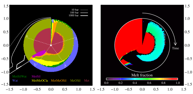
Figure 4: Interior structure (left) and interior melting degree (right) of our Earth analogue shown with time from 0 to 5 Myr represented by the angle. The distance from the centre is normalized by the instantaneous planetary radius. Heating due to decay of ²⁶Al initially leads to melting of the primitive MetSilWat material to form clay beneath a layer of ice. Further heating leads to full interior differentiation within 0.3 Myr. As the radiogenic energy runs out, the continued accretion leads to the emergence of a thick clay mantle overlaid by a massive surface ocean after 3 Myr. The accretion energy finally becomes high enough, after approximately 3.4 Myr, for a run-away greenhouse effect in the ocean-atmosphere system to heat the surface to above the melting temperature of silicates; this leads to a wholesale differentiation of the planet into a silicate mantle and a metal core. The contour lines show the 10, 100 and 1,000 bar pressure levels in the outgassed atmosphere.

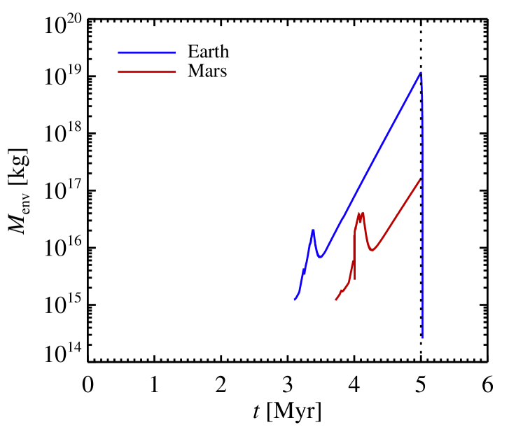
Figure 5: The mass of the envelope as a function of time for Earth and Mars. Mars attracts far less gas from the protoplanetary disc due to its lower mass. The jump in envelope mass at 3.4 Myr for Earth and at 4.0 Myr for Mars is associated with the differentiation of the planets and the outgassing of the massive H₂O and CO₂ atmosphere that is efficient at trapping the accretion heat. The escape of the envelope by XUV irradiation from the star after the end of accretion at 5 Myr is extremely rapid due to the low envelope masses.

2.14 Partitioning of H₂O and CO₂ between magma and solids

As the magma ocean crystallizes, its volatile contents are distributed between the remaining magma and the newly formed solid crystals. Volatiles are typically incompatible, meaning that they partition strongly towards the liquid magma. An equilibrium is obtained when $C_{\rm sol}=kC_{\rm mag}$, with the equilibrium concentration of volatiles in the solids $C_{\rm sol}$ a factor $k$ (generally $\ll 1$) times the concentration of volatiles in the magma $C_{\rm mag}$. We use pressure-dependent values of $k$ for hydroxyl (OH^-) and carbon from Elkins-Tanton (2008). The carbon partitioning is valid for relatively oxidized mantles; we refer to Ortenzi et al. (2020) for an oxygen-fugacity-dependent expression. However, for simplicity we choose to use here the expressions from Elkins-Tanton (2008). For nitrogen, we use the same solid-melt partition coefficient as for carbon. As the total magma mass decreases, the concentration of volatiles in the remaining magma increases and this leads to extensive transfer of volatiles from the mantle to the atmosphere and the core.

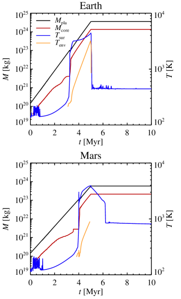
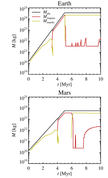
Figure 6: Temporal evolution of mass reservoirs and characteristic temperatures. Left panels: Total mass and core mass (left axis) and surface temperature and envelope temperature (right axis) as a function of time for our Earth and Mars analogues. Right panels: Mass of the planet, the magma ocean and the solid mantle as a function of time. Within the first 3 Myr, the decay of ²⁶Al provides enough energy to drive differentiation into an early core and mantle. The mantle temperature is kept below the liquidus temperature by efficient convective heat transport. A global magma ocean forms when the accretion energy blanketed by the outgassed atmosphere triggers a run-away greenhouse effect. The surface temperature then rises to 4,500 K. The global magma ocean undergoes separation of metal melt from silicate melt, leading to the differentiation into a core and a mantle. The surface temperature falls steeply after the protoplanetary disc dissipates, as the accretion energy vanishes and the hydrostatic gas envelope escapes by stellar XUV irradiation. The surface temperature is nevertheless much higher than the effective temperature because of the greenhouse effect in the massive outgassed atmosphere. The magma ocean crystallizes rapidly after the end of the accretion phase, as its thermal energy is carried upwards by convection and transported through the atmosphere. The base of the magma ocean nevertheless experiences some remelting due to energy transfer from the still molten core (this is visible as spikes in the magma contents after 5 Myr).

3 Heating and differentiation of growing planets

We run simulations for Earth and Mars analogues using for simplicity exponential growth curves. We grow Mars to its modern mass, while Earth is grown only to $0.6\,M_{\rm E}$ because of the later impact with Theia. Theia is constructed to grow to $0.4\,M_{\rm E}$ in the pebble accretion model of Johansen et al. (2021). We present additionally results for Venus in Paper III, focusing mainly on comparing the atmospheric outgassing and escape between Venus, Earth and Mars.

3.1 Temporal evolution of composition and melting degree

We show the evolution of our Earth analogue composition and melting degree in Figure 4. The activity of ²⁶Al is high during the first 2–3 Myr of the evolution and the radiogenic heating leads first to the melting of the ice to form a clay body surrounded by a surface ice layer. Water released from the melting of primitive MetSilWat material is pushed to the surface where it is cooled by the vicinity to the surface. This is followed by interior heating to above the melting temperature of silicates and the separation of the interior into an early core and mantle. However, the draining of the radiogenic energy prohibits further differentiation and instead the accreted layers are heated only enough to forming clay and adding extensive water to the surface ice layer. The effective accretion temperature finally becomes high enough to trigger a run-away greenhouse effect in the coupled ocean-atmosphere system after 3.4 Myr, heating the surface to above the melting temperature of the silicates. This leads to separation of metal melt from silicate melt and the sedimentation of the metal to form the core. The released gravitational energy by early core formation powers additional melting of the remaining solid mantle and the full interior separation of the entire planet into a core and mantle.

3.2 Energetics of differentiation

The gravitational potential energy difference of a blob of metal with mass $m_{\rm met}$ falling from the surface of a protoplanet with mass $M$ and radius $R$ to the core-mantle boundary at radius $R_{\rm c}$ is

$$\Delta E=\frac{GMm_{\rm met}}{R}\left[\frac{3}{2}-\frac{1}{2}\left(\frac{R_{\rm c}}{R}\right)^{2}\right]-\frac{GMm_{\rm met}}{R}\,.$$ (16)

This energy release must be equated with the temperature increase of both the metal (of mass $m_{\rm met}$) and of the silicate component co-accreted with the metal (of mass $m_{\rm sil}$),

$$\Delta E=c_{\rm met}m_{\rm met}\Delta T+c_{\rm sil}m_{\rm sil}\Delta T\,.$$ (17)

In the limit $R_{\rm c}\ll R$ we can write the temperature increase as

$$\Delta T=\frac{GM}{2R(c_{\rm met}+c_{\rm sil}m_{\rm sil}/m_{\rm met})}=1.1\times 10^{4}\,{\rm K}\left(\frac{M}{M_{\rm E}}\right)^{2/3}\left(\frac{\rho}{\rho_{\rm E}}\right)^{1/3}\,.$$ (18)

Here we normalized to the compressed density of Earth, $\rho_{\rm E}$, and used $c_{\rm met}=800\,{\rm J\,kg^{-1}\,K^{-1}}$, $c_{\rm sil}=1200\,{\rm J\,kg^{-1}\,K^{-1}}$, and $m_{\rm sil}/m_{\rm met}=0.62/0.38$ (this includes the full S inventory of the metal, see Paper I). The temperature increase is reduced to $\Delta T\approx 2.4\times 10^{3}\,{\rm K}$ at $M=0.1M_{\rm E}$ and $\Delta T\approx 500\,{\rm K}$ at $M=0.01M_{\rm E}$. The initial fall from infinity to the surface releases twice the energy per mass compared to the subsequent descent of the metal to the core. Since this fall affects the entire mass budget, the accretion to the surface has the potential to heat approximately four times more than the metal descent (Rubie et al., 2015b). Part of this energy is nevertheless carried away through the atmosphere and envelope. The initial differentiation in our model is mainly driven by the penetration into the solid mantle of the metal that melted at the surface. As the planet grows, the trapped accretion energy suffices to melt metal already at its arrival at the surface and the descent to the core only serves to heat the molten metal additionally.

3.3 Envelope mass

We show the mass of the gas envelope attracted from the protoplanetary disc in Figure 5. Earth grows massive enough to attract a significant envelope after 3 Myr of evolution after reaching approximately 0.01 $M_{\rm E}$. The mass then increases rapidly as the Bondi radius $R_{\rm B}=GM/c_{\rm s}^{2}$ expands with increasing mass, peaking at over $10^{19}\,{\rm kg}$. The gas is nevertheless removed very rapidly by XUV irradiation from the young star after the dissipation of the protoplanetary disc. In contrast, the small mass of Mars prevents accretion of any significant gas envelope.

3.4 Core mass and surface temperature

In Figure 6 we show the masses of the planet, core, magma ocean and crystallized mantle, as well as the surface temperature and envelope temperature, as a function of time for our Mars and Earth analogues. Accretion of new layers of primitive, ice-rich material in the first million years leads to rapid melting, outgassing and loss of water. This is visible as intermittent temperature spikes that are caused by our discrete mass accretion scheme (see Paper I).

The core mass increases with time during the first 3 Myr, but the depletion of the ²⁶Al reservoir then prevents further differentiation. The outgassed atmosphere nevertheless undergoes a run-away greenhouse effect as the effective accretion temperature reaches approximately 300 K. This leads to a rapid melting of the mantle and formation of a core containing the bulk iron budget of the planet. The magma ocean crystallizes rapidly after the end of the accretion phase. This leads to the formation of an early mantle with a melting degree of $\varPhi\approx 0.4$ where the thermal conductivity falls dramatically below the fully molten value. The rapid magma ocean crystallization of Mars within a million years after the end of accretion agrees well with age measurements of zircons from martian meteorites (Bouvier et al., 2018; Zhu et al., 2022).

To illustrate the importance of the outgassed atmosphere in facilitating differentiation by thermal blanketing, we show in Figure 7 the core mass fraction as a function of planetary mass for our Earth model. We compare in the figure the model including both the atmosphere and the envelope with a calculation where we include only the hydrostatic gas envelope connected to the protoplanetary disc. Ingassing from contact between such an envelope and the magma ocean has been proposed to explain the water D/H ratio of Earth (Wu et al., 2018) as well as the presence of noble gases of solar composition in the deep mantle (Williams & Mukhopadhyay, 2019). In the absence of a blanketing atmosphere, the protoplanet must grow to approximately 0.3 $M_{\rm E}$ before the surface temperature reaches a high enough energy to melt the mantle and separate metal from silicates. This contrasts with the ten times lower critical differentiation mass of approximately $0.02$ $M_{\rm E}$ when the outgasssed atmosphere is included in the calculations. Therefore a small planet like Mars could only differentiate through the blanketing effect of the outgassed atmosphere, while Earth and Venus are large enough to differentiate from the heat trapped by the hydrostatic envelope alone.

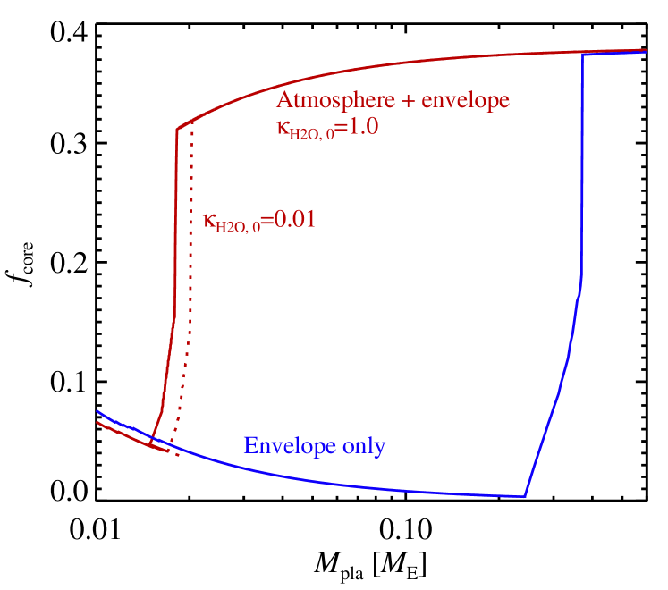
Figure 7: A comparison of the core mass fraction as a function of the accreted mass between the standard model, where we include both the outgassed atmosphere and the hydrostatic envelope connected to the protoplanetary disc, and an additional calculation where we do not include the blanketing effect of the outgassed atmosphere. Neglecting the atmosphere raises the critical planet mass for differentiation by a factor of 10 from approximately $0.02$ $M_{\rm E}$ to $0.3$ $M_{\rm E}$. We also show the evolution of the core mass fraction for a water opacity level 100 times lower than our nominal value. The rapid increase of the accretion luminosity with mass means that even a substantial lowering of the opacity translates to only a small increase in the critical mass that triggers the run-away greenhouse effect and commences differentiation.

3.5 Atmosphere structure

The structure of the planetary atmosphere and envelope goes through many phases during the accretion. We show the pressure-temperature relation in Figure 8 for four illustrative times. During the accretion phase, the hydrostatic gas envelope exerts a pressure on the atmosphere that increases with the mass of the protoplanet and hence with time. The temperature at the base of the envelope is larger than the critical temperature of water, hence water is always in gaseous form in the later stages of the accretion. At $t=5.0$ Myr the pressure reaches $10^{4}$ bar and the temperature $6,000$ K at the surface. The atmospheric pressure is here dominated by SiO vapour while the water vapour constitutes only a small fraction of the pressure. After the dissipation of the protoplanetary disc, the envelope pressure is released and the conditions at the atmosphere’s photosphere, where radiation can leave freely to space, drop down to the effective temperature of the planet under solar irradiation. The first water cloud layers form here as the partial pressure of water crosses over the saturated vapour pressure line.

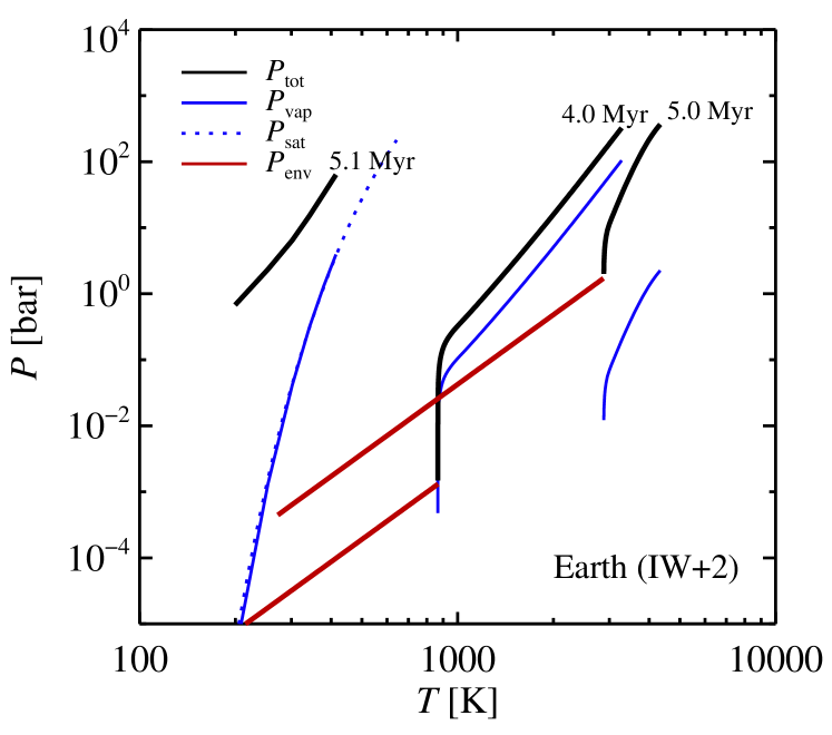
Figure 8: The pressure as a function of temperature for our Earth analogue at three selected times. Before the dissipation of the protoplanetary disc, at $t=4.0$ Myr and $t=5.0$ Myr, the atmosphere connects to the envelope at a pressure and temperature that increases with time as the hydrostatic envelope becomes more massive. The removal of the gas envelope after disc dissipation at $t=5.0$ Myr leads to a much lower pressure and temperature at the photosphere of the isolated planet. The partial pressure of water vapour (thin blue line) follows the shape of the atmospheric pressure for high temperatures (translated down in pressure to reflect the water vapour mixing ratio) and the saturated pressure (dotted blue line) for low temperatures.

The partial pressures of the considered atmospheric components at the surface are shown in Figure 9. The onset of the run-away greenhouse effect in the water component is visible after 3 Myr as a spike in the partial pressure of water. The subsequent emergence of the magma ocean leads to efficient reburial of the H₂O in the magma followed by a slow increase of both SiO and O₂ pressure in the atmosphere. The increase in O₂ pressure is due to the increase of the iron-wüstite buffer in the top of the magma ocean with increasing temperature. The SiO/O₂ atmosphere ‘condenses’ back onto the magma ocean after the stop of the accretion phase. This is followed by the outgassing of the primordial atmosphere of the planet, dominated by CO₂, CO and H₂O as set by the assumption of oxidation stage fO2 = IW + 2 in the mantle. The gradual reduction of the magma volume leads to outgassing first of N- and C-bearing species, while the high solubility of water means that this molecule is outgassed mainly towards the end of the magma ocean crystallization phase (Bower et al., 2022).

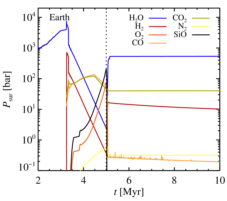
Figure 9: The partial atmospheric surface pressure for all the considered atmospheric components for our Earth analogue. The water pressure includes here both the vapour atmosphere and the underlying water ocean. The initial spike in water pressure is due to the run-away greenhouse effect caused by the accretion energy. This initial outgassed atmosphere is thereafter dissolved in the magma ocean and replaced by an atmosphere with important contributions from SiO (from evaporation of the magma ocean) and O₂ (from the iron-wüstite buffer in the magma ocean). The cessation of the accretion energy after 5 Myr leads to a rapid decline of the SiO/O₂ atmosphere, followed by an outgassing of the final atmosphere dominated by CO₂ and H₂O.

3.6 Interior temperature and magma ocean crystallization

The interior temperature evolution of our Earth analogue is shown in Figure 10. The space-time plot shows the instantaneous value of the temperature at times up to 10 Myr. The early core formation is visible as a region of 2,000 K within the growing planet. This is followed by cold accretion of material that only reaches the melting temperature of water but not the differentiation temperature. The radius of the planet falls as the run-away greenhouse effect sets in after 3.4 Myr and transfers all the water from the surface ocean to the supercritical steam atmosphere. This is followed by the heating of the planet from the surface and downwards, an effect which is exacerbated by the sedimentation of iron droplets that release gravitational binding energy. After the accretion terminates, the mantle temperature falls rapidly to near the solidus temperature of the silicates.

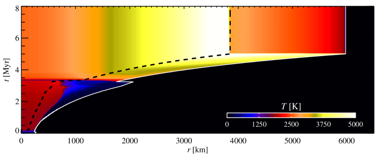
Figure 10: Temperature map of our Earth analogue as a function of distance form the centre and time. The black dashed line indicates the size of the core, while the planetary radius is indicated with a thin white line. The accretion of cold material, unable to heat to differentiation by ²⁶Al decay, is visible as a blue clump between 2 Myr and 3.5 Myr. The planetary radius falls significantly as the water ocean is lost to the run-away greenhouse effect after 3.4 Myr. The termination of accretion after 5 Myr is followed by a slow cooling first and then by rapid cooling when the gas envelope escapes after 7 Myr. This leads to a decrease of the mantle temperature towards the solidus value where the heat conductivity due to convective heat transport drops dramatically. The core remains in a hot state after mantle cooling, since the hot outer core stabilizes the liquid metal against convective heat transport.

The mode of closing of the magma ocean plays an important role in distributing volatiles between the mantle and the atmosphere (Elkins-Tanton, 2008). The magma ocean is most prone to solidify from the bottom, due to higher solidus temperature at higher pressure and to the foundering and remelting of any emerging crust into the liquid magma below (Weiss & Elkins-Tanton, 2013). We hence assume that a magma ocean extending up to at least 70% of the planetary radius is in contact with the atmosphere irrespective of whether a lid forms in the numerical simulations. We close the contact between the mantle and the core after a solid layer forms at the bottom of the mantle with a thickness of at least 10% of the planetary radius.

We show in Figure 11 the evolution of the melting degree of the core and the mantle after the gas envelope has been removed and the liquidus temperature is first reached in the magma ocean. The magma ocean of our Earth analogue crystallizes initially from surface down and later from the core and up. This traps a small melt region in the middle of the mantle that slowly approaches the melting degree $\varPhi\approx 0.4$ where mantle viscosity increases dramatically (see Paper I). Our Mars analogue, in contrast, crystallizes its magma ocean from the bottom up.

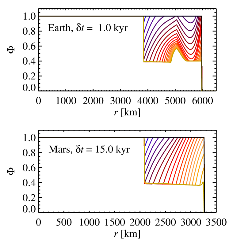
Figure 11: The interior melting degree $\varPhi$ of our Earth and Mars analogues in steps of 1 kyr (Earth) and 15 kyr (Mars) after first reaching the magma ocean liquidus after termination of accretion. Earth experiences rapid crystallization and a solidification that propagates first from the top of the magma ocean and down and later from the bottom up. A small region is left in the middle mantle with a melting degree that slowly approaches $\varPhi=0.4$ below which the magma viscosity increases strongly. The Mars analogue crystallizes its magma ocean from the bottom up and more slowly, due to thermal blankering by its thick H₂-rich atmosphere that slows the cooling of the magma ocean.

3.7 Evolution of the water reservoirs

We will analyse the volatile (H, C, O, and N) contents of core, mantle, and atmosphere, as well as the early atmospheric escape, in more detail in Paper III. Here we describe only on the fate of water within the growing planets. Our planets accrete approximately $2\times 10^{22}$ kg of water from icy pebbles (Johansen et al., 2021), which corresponds to 15 Earth oceans. This amount is independent on the final mass of the planet, so Mars and Earth accrete the same amount of water despite the much lower mass of Mars. We show in Figure 12 the mass of the water in the different reservoirs. Before the run-away greenhouse effect, most of the water resides in the surface ocean and the clay mantle. This water is lost to the atmosphere as supercritical steam after the run-away greenhouse effect sets in. However, the formation of the global magma ocean opens a new reservoir for water – and most of the water dissolves in the magma ocean from where a large fraction also enters the core. The core of Earth can hold much more water than the smaller core of Mars; hence 95% of the water resides in the end in the core of Earth, while Mars’ core holds a factor two less water. The crystallization of the magma ocean after the accretion terminates pushes the incompatible water back into the atmosphere. We assume here that the upper mantle of Earth has an oxygen fugacity of IW+2 (Armstrong et al., 2019; Sossi et al., 2020; Deng et al., 2020), while Mars is much more reduced with IW-2 because its magma ocean does not reach depths where Fe³⁺ is produced in reactions between less-oxidized Fe²⁺. Hence Earth outgasses approximately two modern oceans of water, while Mars outgasses mainly hydrogen that is lost by hydrodynamic escape. The composition and escape of the outgassed atmosphere are discussed in details in Paper III.

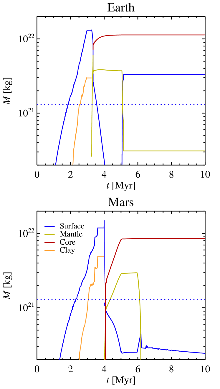
Figure 12: The mass of water in different reservoirs as a function of time (top: Earth, bottom: Mars). Before the onset of the run-away greenhouse effect, most of the water resides in the massive surface layer and in the clay mantle below. The majority of the water is dissolved into the newly formed magma ocean and core when the planets differentiate by the accretion energy. The crystallization of the magma ocean after 7 Myr leads to the release of approximately two modern Earth oceans of water on Earth, while the reduced mantle of Mars leads to outgassing of far less water.

We have assumed that the partitioning between core, mantle and atmosphere takes place only when the magma ocean melt fraction is higher than a threshold value of $\varPhi=\varPhi_{\rm melt}=0.5$ (see Section 2.8). This choice is motivated by a transition from liquid behaviour to solid behaviour around a critical melt fraction of $\varPhi=0.4$ (Monteux et al., 2016, see discussion in paper I). To test the influence of this choice on the partitioning of water, we show in Figure 13 the mass of water stored in the core, mantle and atmosphere for the nominal choice of $\varPhi_{\rm melt}=0.5$ compared to $\varPhi_{\rm melt}=0.3$ and $\varPhi_{\rm melt}=0.7$. When the threshold melt fraction $\varPhi_{\rm melt}$ is lowered, the magma ocean formally can not crystallize after accretion, since the collapse of the heat conductivity at $\varPhi\approx 0.4$ prevents further, rapid cooling. Increasing instead the threshold melt fraction to $\varPhi_{\rm melt}=0.7$ leads to a surge in the mantle reservoir of water, as the water concentration “freezes” in at a higher magma mass that can hence hold more water. The atmospheric reservoir is therefore reduced by a factor of approximately two compared to the nominal choice of melt fraction threshold.

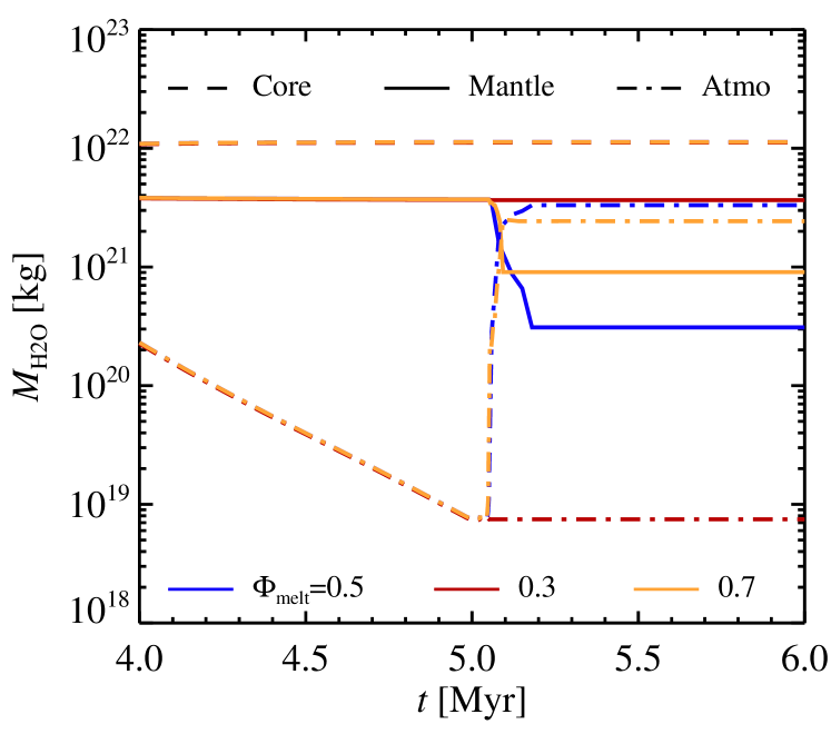
Figure 13: The mass of water in the core, mantle and atmosphere reservoirs for three different choices of the threshold melt fraction $\varPhi_{\rm melt}$ above which the magma ocean is considered liquid and can hence exchange volatiles with the core and the atmosphere. The core reservoir is relatively unaffected by this choice and holds in all cases the dominant water mass. Lowering the threshold fraction to 0.3 means that the magma ocean does not formally crystallize and hence the mantle reservoir cannot outgas efficiently to the atmosphere. Increasing instead to $\varPhi_{\rm melt}=0.7$ causes less outgassing than the nominal choice of $\varPhi_{\rm melt}=0.5$, since the volatile exchange with the atmosphere ceases at a higher magma mass that can thus store more volatiles. This reduces the atmospheric reservoir of water by a factor of approximately two.

3.8 Conditions for core-mantle separation

The concentrations of moderately and weakly siderophile elements in the mantle of Earth can be used to constrain the pressure at which metal and silicate melts equilibrated their elemental concentrations. Mann et al. (2009) concluded that the differentiation pressure must have exceeded 30–60 GPa to match their experimental measurements of the metal-liquid partition coefficients of a range of siderophile elements. Badro et al. (2015) obtained similar constraints based on the contents of Si and O in the terrestrial core. The pressure at the core-mantle boundary of our Earth analogue with a mass of $0.6\,M_{\rm E}$ is 60 GPa, in good agreement with the conclusion of Mann et al. (2009) and Badro et al. (2015). However, the core-mantle boundary pressure after the moon-forming giant impact must have been similar to the modern value (136 GPa) and this raises the question to what degree the metal of the core of Theia equilibrated with the mantle material of Earth and Theia during the collision. We discuss mantle-core equilibration of W isotopes during the moon-forming impact in the next section.

The temporally evolving oxidation state of the magma ocean also affects the partitioning of elements such as Si and O between liquid metal and silicates. Badro et al. (2015) presented mantle-core partitioning results for a range of temporal profiles of the FeO fraction in the magma. They found the best matches to the abundance of siderophile elements in the mantle and the density of the core (lowered due to incorporation of lighter elements) for FeO mantle fractions initially around 20–25% and falling towards 6% with time, with similar pressure constraints as Mann et al. (2009). This increasingly reduced mantle is in good agreement with the pebble accretion model where most of the FeO is produced by water flow during the earliest accretion and subsequently thinned out by accretion of dry pebbles with a high content of metallic iron (see Paper I). This model contrasts with the prevailing view that Earth became increasingly oxidized during its accretion (Wade & Wood, 2005; Rubie et al., 2015a). For the weakly and moderately siderophile elements in the mantle of Mars, modelling is generally consistent with differentiation under reducing conditions (with oxygen fugacity around ${\rm IW}-1.5$ Righter & Chabot, 2011; Rai & van Westrenen, 2013). This corresponds roughly to the inferred FeO mass fraction in the mantle of Mars of 18% (Robinson & Taylor, 2001) which we reproduced in the pebble accretion model in Paper I.

4 Hf-W model fits

Hf is a lithophile (rock-loving) element with an unstable isotope ¹⁸²Hf that decays to ¹⁸²W with a half-life of approximately 8.9 Myr. Since W is moderately siderophile (iron-loving), the evolution of the abundances of Hf and W in the mantle and core of our Earth analogue can be linked to measurements of the abundances of these elements in Earth’s mantle and in chondrites, in order to infer the consistency of our model of rapid terrestrial planet formation against those measurements. We follow Yin et al. (2002) and define the excess of ¹⁸²W relative to ¹⁸³W in the mantle of our model planets as

$$\epsilon_{\rm W}=\left[\frac{(^{182}{\rm W}/^{183}{\rm W})_{\rm model}}{(^{182}{\rm W}/^{183}{\rm W})_{\rm Earth}}-1\right]\times 10^{4}\,.$$ (19)

Here $(^{182}{\rm W}/^{183}{\rm W})_{\rm Earth}\approx 1.85130$ is the measured ratio in Earth’s mantle, which by this definition has $\epsilon_{\rm W}=0.0$. The initial value at the birth of the Solar System, before substantial ¹⁸²Hf decay, was $\epsilon_{\rm W,SS}=-3.5$ and the modern value for undifferentiated chondritic material is $\epsilon_{\rm W,CHUR}=-2.0$. The low value of $\epsilon_{\rm W}$ for Earth, compared to, for example, Vesta with $\epsilon_{\rm W}=17$ (Jacobsen, 2005), has been used to argue for a protracted Earth accretion taking at least 34 Myr (Kleine & Walker, 2017), in agreement with traditional planetesimal accretion models (Raymond et al., 2004), or for rapid accretion within 10 Myr (Yin et al., 2002; Yu & Jacobsen, 2011), followed by equilibration in the moon-forming impact. This giant impact could have significantly lowered the $\epsilon_{\rm W}$ value by interaction of Earth’s mantle with material from the ¹⁸²W-poor core of the impacting planetary body (see discussion below).

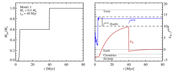
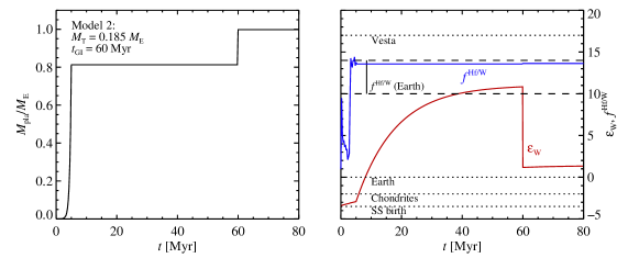
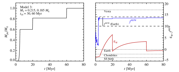
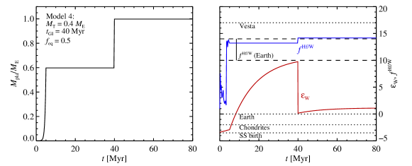
Figure 14: Comparisons of four models of Earth formation by rapid pebble accretion to the Hf-W isotope data for Earth. The top panels (Model 1) shows results for our nominal impactor mass of $0.4\,M_{\rm E}$ colliding with proto-Earth after 40 Myr. The excess of ¹⁸²W in the mantle builds up a to a value of nearly 10 before the interaction of the mantle material with the impacting Theia core delivers enough ¹⁸³W to bring the $\epsilon_{\rm W}$ value down towards the measured data. The second panel (Model 2) show instead the effect of lowering the impactor to $0.185\,M_{\rm E}$ (we use here our Venus analogue for the proto-Earth model). We set the impact to occur after 60 Myr to avoid subsequent build up of ¹⁸²W in the mantle, but the impactor mass is too low to bring the model to agree with the measured $\epsilon_{\rm W}$ of Earth. The canonical impactor model is reconciled with the Hf-W system in the third row (Model 3) where we include two giant impacts: an early impact at 20 Myr removes the initial ¹⁸²W excess and the second (moon-forming) giant impact brings the subsequent mantle ingrowth of ¹⁸²W down to the modern terrestrial value. Finally, the lower panels (Model 4) show the effect of lowering the equilibration efficiency to $f_{\rm eq}=0.5$. The $\epsilon_{\rm W}$ value ends above the terrestrial value in this case.

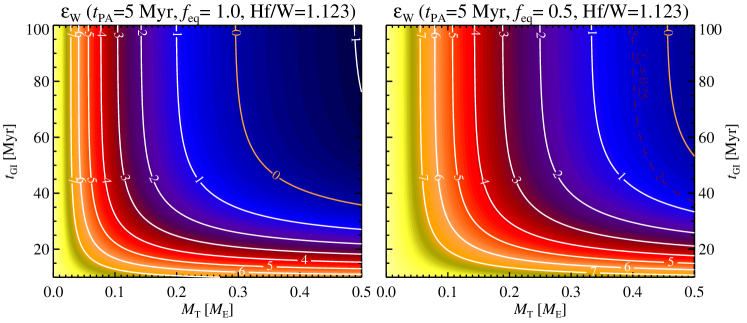
Figure 15: Contour plot of the ¹⁸²W excess of Earth’s mantle after 200 Myr of evolution, as a function of the impactor mass ($M_{\rm T}$) and the time of the giant impact ($t_{\rm GI}$). The left plot shows results for complete equilibration between the core of Theia and proto-Earth, while the right plot shows results for 50% equilibration (i.e., 50% of the core of Theia merges directly with Earth’s core). The pebble accretion time-scale has been set to $t_{\rm PA}=5$ Myr in both cases. The $\epsilon_{\rm W}=0$ value of Earth is consistent with the pebble accretion model for an impactor mass between $0.3\,M_{\rm E}$ and $0.5\,M_{\rm E}$ and a fully equilibrating impact that occurs at least 35 Myr after the formation of the Sun. Lowering the equilibration to 50% requires an impact between two nearly equal-mass bodies to occur after at least 50 Myr. The so-called canonical model, with an impactor of 10% Earth mass (Canup & Asphaug, 2001), is excluded in both cases which instead favour an impactor with a similar mass as proto-Earth (Canup, 2012). A very low equilibration factor of $f_{\rm eq}=0.25$ yields $\epsilon_{\rm W}$ values larger than 1.5 for all impactor masses; the $\epsilon_{\rm W}=2.0$ contour for $f_{\rm eq}=0.25$ is indicated with a black dashed line.

4.1 Modelling the Hf-W system

We postprocess the evolution of the Hf-W system of our Earth analogue by dividing the accretion into several time-steps and calculating for each time-step how the accreted W distributes between the core and the mantle and how the abundance of ¹⁸²W in the mantle increases by the decay of ¹⁸²Hf. We assume that an accreted mass $\delta M$ consists of a fraction $f_{\rm Sil}=68\%$ silicates and a fraction $f_{\rm Met}=32\%$ metal and equilibrates its contents of W with a whole-mantle magma ocean. The accreted core mass is $\delta M_{\rm core}=f_{\rm Met}\delta M$ and the amount of W accreted into the core is

$$\delta M_{\rm W}^{\rm(core)}=C_{\rm W}^{\rm(Met)}\delta M_{\rm core}\,.$$ (20)

Here $C_{\rm W}^{\rm(Met)}$ is the equilibrium concentration of W in the metal melt. Knowledge of the total amount of accreted W and its partition coefficient $D=C_{\rm W}^{\rm(Met)}/C_{\rm W}^{\rm(Sil)}$ yields the connection

$$M_{\rm W}^{\rm(Sil)}+\delta M_{\rm W}=C_{\rm W}^{\rm(Sil)}(M_{\rm Sil}+\delta M_{\rm Sil})+C_{\rm W}^{\rm(Met)}\delta M_{\rm core}\,.$$ (21)

Here $M_{\rm W}^{\rm(Sil)}$ is the existing W in the mantle, $\delta M_{\rm W}$ is the accreted W, $M_{\rm Sil}$ is the mass of the mantle and $\delta M_{\rm Sil}$ is the accreted silicates. Replacing $C_{\rm W}^{(\rm Sil)}=C_{\rm W}^{\rm(Met)}/D=\delta M_{\rm W}^{\rm(core)}/(D\delta M_{\rm core})$ yields the W addition to the core

$$\delta M_{\rm W}^{\rm(core)}=\frac{M_{\rm W}^{\rm(Sil)}+\delta M_{\rm W}}{1+(M_{\rm Sil}+\delta M_{\rm Sil})/(D\delta M_{\rm core})}\,.$$ (22)

This expression covers both single accretion event where the whole impactor (core and mantle) equilibrates with the whole mantle of the planet before the metal component sinks to the core, as well as continuous pebble accretion where $\delta M_{\rm Sil}\ll M_{\rm Sil}$ due to the time-stepping. In that limit the accretion expression tends towards

$$\delta M_{\rm W}^{\rm(core)}\rightarrow D\frac{M_{\rm W}^{\rm(Sil)}}{M_{\rm Sil}}\delta M_{\rm core}\,.$$ (23)

The partition coefficient $D$ of W between metal melt and silicate melt is relatively uncertain and depends on both equilibration pressure, temperature and the presence of other elements such as O, S and C in the melt (Walter & Cottrell, 2013; Jennings et al., 2021). We therefore for simplicity take $D=25$; this gives a good match to the Hf/W overabundance of Earth relative to the chondritic value, $f^{\rm Hf/W}=12\pm 2$ (Jacobsen, 2005).

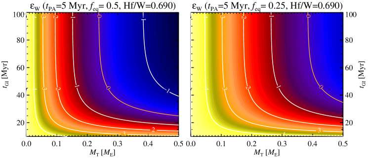
Figure 16: The final ¹⁸²W excess as a function of impactor mass and impact time, for an initially reduced value of Hf/W=0.69 that may represent the inner Solar System composition (Nimmo & Kleine, 2007). The lower amount of ¹⁸²Hf makes it easier for the impactor core material to transport excess ¹⁸²W to the combined post-giant-impact core. Hence the pebble accretion time-scale of 5 million years is here consistent with core-mantle equilibration factors as low as $f_{\rm eq}=0.5$ (left plot) and $f_{\rm eq}=0.25$ (right plot).

We show the results of our Hf-W modelling in Figure 14. The results depend strongly on the choice of impactor mass and the degree of equilibration between the impactor core and the mantle material. To bracket the realm of possible matches to the Hf-W data, we consider the mass of Theia to have been either $0.4\,M_{\rm E}$ (our nominal case) or $0.185\,M_{\rm E}$. In the latter case we use our Venus analogue as a model of proto-Earth before the collision. We can match the measured value of $\epsilon_{\rm W}$ for Earth to rapid core formation on Earth within 5 Myr, which drives $\epsilon_{\rm W}$ up to 9–10, followed by a giant impact happening at the earliest after $t=35$ Myr where the impactor equilibrates fully with Earth and hence drives down $\epsilon_{\rm W}$ to the modern value. Lowering the impactor mass to $0.185\,M_{\rm E}$ precludes any match to the data, since the impactor does not contain enough W in its core to equilibrate Earth’s value of $\epsilon_{\rm W}$ down to 0.

4.2 Testing impactor mass and timing

The consistency of the rapid pebble accretion model for Earth formation with the Hf-W system clearly hinges on the exchange of W isotopes between the core of the moon-forming impactor and the mantle of Earth (Rudge et al., 2010). In Figure 15 we map the final value of the ¹⁸²W excess as a function of the mass of the impactor and the time of the giant impact. We used here a simple growth model where the pebble accretion rate scales with planetary mass as $\dot{M}\propto M^{2/3}$, approximating growth in the 2-D Hill regime of pebble accretion (Lambrechts & Johansen, 2012). This gives the growth function $M(t)=(3Kt)^{1/3}$, where $K$ is a growth constant that is fixed by requiring that the planet reaches its pre-impact mass $M_{1}$ after a time of $t_{1}=5\,{\rm Myr}$. Planetesimal-driven models typically use an exponentially decaying mass curve (Kleine et al., 2009); we have verified that the specific choice of growth curve affects the final $\epsilon_{\rm W}$ value by less than 0.1.

Figure 15 shows results for core-mantle equilibration of 100% and 50% in the giant impact. In the latter case, half of the core of Theia merges with the core of Earth without exchanging any isotopes with the mantle. For full equilibration, the pebble accretion model is consistent with an impactor mass between $0.3\,M_{\rm E}$ and $0.5\,M_{\rm E}$ happening at least 35 Myr after the formation of the Sun. For the lower end of this range, the giant impact time can be very long, since the impact itself drives $\epsilon_{\rm W}$ to near zero. A young age of the Moon is also consistent with Pb-Pb dating yielding moon formation $\sim$150 Myr after the formation of the Solar System (Connelly & Bizzarro, 2016). Lowering the equilibration to 50%, consistency of the pebble accretion model with the Hf-W system requires two nearly equal-mass planets to collide after at least 50 Myr.

Figure 15 used the initial ratio Hf/W$=1.123$ measured for carbonaceous chondrites (Yin et al., 2002). Ordinary chondrites, representing the composition of the inner Solar System, display a range of lower and higher values. We follow Nimmo & Kleine (2007) here and rerun our model using the H-chondrite value Hf/W$=0.7$. The results are presented in Figure 16. The pebble accretion time-scale of 5 million years is now consistent with equilibration degrees as low as $f_{\rm eq}=0.5$ and $f_{\rm eq}=0.25$. The isotopic composition of Earth and Mars in their major lithophile elements can be matched with a mixture of inner Solar System and outer Solar System material (Trinquier et al., 2009; Warren, 2011; Schiller et al., 2018). The starting value of Hf/W for Earth and Mars was therefore likely between the H-chondritic value and the carbonaceous chondrite value. Figures 15 and 16 thus represent endmember solutions for pure inner or outer Solar System compositions. We conclude overall that the metal-silicate equilibration degree in the moon-forming giant impact should not be much below the range of 25%-50%, in order for a 5-million-years accretion time-scale to be in agreement with the Hf-W system.

4.3 Mixing degree in the giant impact

The very similar ratio of ¹⁸²W/¹⁸⁴W measured on Earth and the Moon speak for efficient mixing of impactor and target after the moon-forming impact (Touboul et al., 2007). Any material from the mantle of proto-Earth that experienced equilibration with the impactor must have been efficiently mixed with the material that formed the Moon, in order to explain the similar W isotopic abundances. Alternatively, the value of ¹⁸²W/¹⁸⁴W could have been similar on Theia and proto-Earth. However, such a correspondence would be very unlikely in the traditional giant impact scenario for planetary differentiation, since the two bodies would have experienced stochastic impact histories. Mars has an elevated value of $\epsilon_{\rm W}$ relative to Earth, which indicates very rapid core formation within a few Myr after the formation of the Solar System (Dauphas & Pourmand, 2011). Such an impactor would require extensive equilibration and mixing in the impact to drive $\epsilon_{\rm W}$ towards zero for both the Earth and the Moon.

Alternatively, Earth and Theia could have both formed their cores after the extinction of ¹⁸²Hf, but then the Earth-Moon system should have remained chondritic $\epsilon_{\rm W}$ ($=-1.9$) and the measured elevation is unexplained. The slight offset of the ¹⁸²W/¹⁸⁴W of the Moon compared to Earth (at the 20 ppm level, or 0.2 $\epsilon$ units) could be a signature of a later veneer of chondritic material that preferentially enriched the more massive Earth compared to the Moon (Touboul et al., 2015; Kruijer & Kleine, 2017).

Dahl & Stevenson (2010) used fluid dynamical models of planetesimals impacting a larger planet to show that the emulsification of the iron core of the impactor becomes increasingly inefficient as the impactor mass increases. However, a collision between two nearly equal-sized planets, particularly if not directly head on, would lead to a large-scale mixing of the two bodies (Canup, 2012). The core of the impactor is sheared into multiple smaller components during the first stage of the collision and these smaller metal blobs subsequently undergo efficient emulsification while sedimenting to the core of the combined planet (Deguen et al., 2014; Genda et al., 2017). Laboratory experiments show that taking into account the inertia of the impactor dramatically increases the degree of mixing (Landeau et al., 2021). Maas et al. (2021) utilized convective magma ocean models and concluded that the convection and rotation of the planet leads to much larger fractions of equilibrated volume than previously estimated and that the equilibrated volume fraction increases with increasing impactor mass. Hence a large degree of equilibration between a planetary-mass impactor and proto-Earth following a planetary instability seems supported by hydrodynamical simulations of impactor core emulsification.

5 Discussion and implications

The outgassing of volatiles to form a thick atmosphere during the planetary accretion phase is key to achieving interior differentiation of terrestrial planets. Pebbles deposit their accretion energy at the planetary surface and this energy radiates away through the hydrogen envelope attracted from the protoplanetary disc relatively easily. However, the outgassed atmosphere of mainly H₂O and CO₂ provides a strong thermal blanketing that traps the accretion energy and heats the surface to well above the liquidus of the silicates. Magma oceans thus form as a natural evolution step in the planet formation process once the protoplanet reaches a mass above approximately 2% of an Earth mass. We nevertheless demonstrate that the differentiation threshold mass has a weak dependency on the assumed opacity of the atmospheric constituents. Future models using frequency-dependent radiative transfer with realistic opacity tables will therefore be useful to pin down more precisely the value of the threshold mass for differentiation.

The trapped accretion energy would only penetrate slowly downwards through the magma ocean. However, a more important source of mantle heating comes from the continuous separation of metal melt from silicate melt and sedimentation of the metal melt to the bottom of the magma ocean. This releases enough gravitational potential energy to rapidly expand the magma ocean all the way down to the metal core. Subsequent accreted pebble material experiences rapid separation of metal from silicates at the top of the magma ocean and fast sedimentation to join the core.

The consistency of Earth’s Hf-W system with the rapid accretion time-scale of ${<}10$ Myr followed by an additional major mass contribution from the moon-forming impactor was highlighted by Yu & Jacobsen (2011). We have demonstrated here a match between the Hf-W system and a pebble accretion model with accretion time-scale as short as 5 Myr, followed by a collision with a planetary body of mass in the range between $0.3\,M_{\rm E}$ and $0.5\,M_{\rm E}$, in agreement with high-mass and high-angular momentum models for the moon-forming giant impact as well as the necessity for extensive mixing of impactor and target (Canup, 2012). In this view, the moon-forming impact is not the last of a series of giant impacts that formed Earth, but rather the result of an instability in a primordial terrestrial planet system that contained an additional planet between Earth and Mars.

We have nevertheless found that impactor masses consistent with the Hf-W system depend strongly on the assumed initial ratio of Hf/W as well as on the degree of equilibration between the core of the impactor and the mantle of proto-Earth. A low value of Hf/W – consistent with measurements of ordinary chondrites (Nimmo & Kleine, 2007) – allow impactor masses as low as $0.2\,M_{\rm E}$, more akin to the canonical impact model (Canup & Asphaug, 2001), or low an equilibrium fraction as low as $f_{\rm eq}=0.25$.

The preservation of anomalous ¹⁸²W isotope signals in Earth’s deep mantle, expressed by both excesses and deficits relative to the upper mantle composition (i.e. Mundl et al., 2017; Willbold et al., 2011) has been suggested to imply inefficient mixing between Earth and the moon-forming impactor and, hence, speak against a planetary-mass impactor. However, the small ¹⁸²W deficits identified in modern deep-seated mantle plumes are thought to reflect interaction with Earth’s core whereas the ¹⁸²W excesses measured in Archean rocks (Mundl-Petermeier et al., 2020; Rizo et al., 2019) are interpreted to reflect the composition of Earth’s mantle prior to the addition of the late veneer (Willbold et al., 2011; Tusch et al., 2021). As such, the preservation of ¹⁸²W heterogeneities in Earth’s deep mantle does not provide evidence for limited mixing during the moon-forming impact.

Appendix A Numerical scheme for atmospheric luminosity

The planet possesses both an outgassed atmosphere (of mass $M_{\rm atm}$) and an envelope attracted from the protoplanetary disc (of mass $M_{\rm env}$). The goal is to find the luminosity of the planet as a function of the known surface temperature and the disc pressure and temperature boundary conditions (for embedded planets) or the envelope mass (for isolated planets). We assume that the opacity at the disc temperature is $\kappa_{\rm d}$ and that it increases with temperature as $T^{\beta}$ with $\beta=2$. This is only approximately true for the opacity at temperatures below the sublimation temperature of dust, but the radiative-convective boundary typically occurs when the temperature is well below the sublimation temperature.

A.1 Embedded planet

We consider first a planet still embedded within the protoplanetary disc. Here the heat is removed from the planet–atmosphere–envelope system by the temperature boundary condition at the Hill radius. We therefore follow Piso & Youdin (2014) and integrate inwards from the disc boundary condition at the Hill radius. We define the quantities

$$\nabla_{\rm ad} = \frac{\gamma-1}{\gamma}\,,$$ (24)

$$\nabla_{\infty} = \frac{1}{4-\beta}\,,$$ (25)

$$\nabla_{\rm d} = \frac{3\kappa_{\rm d}P_{\rm d}}{64\pi GM\sigma_{\rm SB}T_{\rm d}^{4}}L\,.$$ (26)

Here $\gamma$ is the adiabatic index of the envelope gas, assumed here to be $\gamma=1.4$ valid for molecular hydrogen. The luminosity of the planet is $L$ and $\kappa_{\rm d}$, $P_{\rm d}$ and $T_{\rm d}$ are the opacity, pressure and temperature at the outer boundary. The temperature profile changes from isothermal to adiabatic at the radiative-convective boundary $R_{\rm rcb}$. The pressure at the radiative-convective radius is

$$P_{\rm rcb}=P_{\rm d}\frac{\nabla_{\rm ad}/\nabla_{\rm d}-\nabla_{\rm ad}/\nabla_{\infty}}{1-\nabla_{\rm ad}/\nabla_{\infty}}\,.$$ (27)

The temperature at the radiative-convective boundary follows from integration from the Hill radius through the radiative envelope solution and becomes

$$T_{\rm rcb}=T_{\rm d}\left[\frac{\nabla_{\rm d}}{\nabla_{\infty}}\left(\frac{P_{\rm rcb}}{P_{\rm d}}-1\right)+1\right]^{1/(4-\beta)}\,.$$ (28)

Piso & Youdin (2014) showed that the location of the radiative-convective boundary is close to the Bondi radius $R_{\rm B}=GM/c_{\rm s}^{2}$ with $c_{\rm s}$ denoting the sound speed at the temperature of the outer boundary,

$$R_{\rm rcb}=\frac{R_{\rm B}}{\ln(P_{\rm rcb}/P_{\rm d})}\,.$$ (29)

The temperature at the bottom of the envelope follows integration through the adiabatic envelope,

$$T_{\rm env}=T_{\rm rcb}+\left(\frac{GM}{R}-\frac{GM}{R_{\rm rcb}}\right)\frac{1}{c_{\rm p}}\,.$$ (30)

From $T_{\rm rcb}$, $P_{\rm rcb}$ and $T_{\rm env}$ follows $P_{\rm env}$ by the adiabatic connection $P\propto T^{\gamma/(\gamma-1)}$. All these quantities are therefore given uniquely by the set $(P_{\rm d},T_{\rm d},L)$.

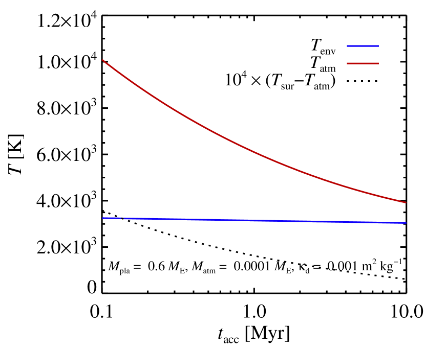
Figure 17: The envelope temperature, atmospheric bottom temperature and surface temperature difference as a function of the accretion time-scale (a measure of the luminosity through $L=GM\dot{M}/R$). The envelope temperature is close to 3,500 K for all values of the accretion time-scale. Matching this temperature at the top of the atmosphere leads to atmospheric temperatures above 10,000 K for short accretion times (high luminosities) and 4,000 K for long accretion times (low luminosities).

This temperature and pressure must then match the temperature and pressure at the top of the outgassed atmosphere. We know $P_{\rm atm}$ from the envelope pressure and the atmospheric mass,

$$P_{\rm atm}=\frac{gM_{\rm atm}}{4\pi R^{2}}+P_{\rm env}\,,$$ (31)

under the assumption that the thickness of the atmosphere is much lower than the planetary radius so that the gravitational acceleration $g$ can be assumed constant. We can then test different values of $T_{\rm atm}$ (the temperature at the bottom of the atmosphere) until the conditions at the top of the atmosphere, where the pressure has fallen to $P=P_{\rm env}$, match the temperature and pressure conditions at the bottom of the envelope. The luminosity is directly related to the surface temperature $T_{\rm sur}$ and the temperature at the bottom of the atmosphere $T_{\rm atm}$ through

$$L_{\rm atm}=4\pi R_{\rm pla}^{2}\sigma_{\rm SB}(T_{\rm sur}^{4}-T_{\rm atm}^{4})\,.$$ (32)

The atmosphere-envelope match is thus obtained at a unique luminosity $L_{\rm atm}$ for a known surface temperature $T_{\rm sur}$.

The outgassed atmosphere consists of multiple chemical species, including water with a tabulated equation of state. The atmospheric integration therefore has no analytical solution. We can nevertheless test our algorithm considering an outgassed atmosphere consisting entirely of CO₂ with an ideal-gas equation of state and an adiabatic index of $\gamma=1.3$. The envelope temperature, atmospheric temperature and surface temperature are shown in Figure 17 for a planetary mass of $M=0.6\,M_{\rm E}$, an atmosphere mass of $M_{\rm atm}=10^{-4}M_{\rm E}$ and a protoplanetary disc opacity of $\kappa_{\rm d}=0.001\,{\rm m^{2}\,kg^{-1}}$. The envelope temperature lies around $T\approx 3,500\,{\rm K}$ for the considered range of accretion time-scales (which define the luminosity). The surface temperature and atmospheric temperature are indistinguishable, reflecting that the effective cooling temperature is much lower than the surface temperature.

A.2 Isolated planet

After the dissipation of the protoplanetary disc, cooling is no longer taken care of by the gas flow outside of the Hill radius. Instead, cooling is directly achieved by loss of radiation from the photosphere. We assume in this case that the hydrogen-helium envelope contracts to form a geometrically thin envelope. We then calculate the photospheric temperature directly from the luminosity, $L=4\pi R^{2}\sigma_{\rm SB}T_{\rm pho}^{4}$. The pressure at the photosphere follows from integration of the hydrostatic equilibrium from $\tau=0$ to $\tau=2/3$, which yields

$$P_{\rm pho}=\frac{(2/3)g}{\kappa_{\rm d}}\,,$$ (33)

where $g$ is the gravitational acceleration at the surface and $\kappa_{\rm d}$ is the opacity of the envelope at the ambient temperature of the now-dissipated protoplanetary disc (which we set to $\kappa_{\rm d}=0.1\,{\rm kg\,m^{-2}}$). The pressure at the bottom of the envelope follows

$$P_{\rm env}=\frac{gM_{\rm env}}{4\pi R^{2}}\,.$$ (34)

The temperature at the bottom of the envelope is then calculated from the adiabatic relation between the photosphere and the surface. We have compared this approach to an algorithm that allows for the envelope to extend upwards to regions of lower gravity and found no significant differences. The geometrically thin assumption is therefore preferred, given its known analytical solution for $P_{\rm env}$ as a function of $M_{\rm env}$. When the envelope has been removed by the XUV irradiation from the star, the outgassed atmosphere is exposed directly to vacuum cooling conditions.