Schwarz methods by domain truncation

Abstract

Schwarz methods use a decomposition of the computational domain into subdomains and need to put boundary conditions on the subdomain boundaries. In domain truncation one restricts the unbounded domain to a bounded computational domain and also needs to put boundary conditions on the computational domain boundaries. In both fields there are vast bodies of literature and research is very active and ongoing. It turns out to be fruitful to think of the domain decomposition in Schwarz methods as truncation of the domain onto subdomains. Seminal precursors of this fundamental idea are ?, ? and ?. The first truly optimal Schwarz method that converges in a finite number of steps was proposed in ? and used precisely transparent boundary conditions as transmission conditions between subdomains. Approximating these transparent boundary conditions for fast convergence of Schwarz methods led to the development of optimized Schwarz methods – a name that has become common for Schwarz methods based on domain truncation. Compared to classical Schwarz methods which use simple Dirichlet transmission conditions and have been successfully used in a wide range of applications, optimized Schwarz methods are much less well understood, mainly due to their more sophisticated transmission conditions.

A key application of Schwarz methods with such sophisticated transmission conditions turned out to be time-harmonic wave propagation problems, because classical Schwarz methods simply do not work then. The last decade has brought many new Schwarz methods based on domain truncation. A review from an algorithmic perspective (?) showed the equivalence of many of these new methods to optimized Schwarz methods. The analysis of optimized Schwarz methods is however lagging behind their algorithmic development. The general abstract Schwarz framework can not be used for the analysis of these methods, and thus there are many open theoretical questions about their convergence. Like for practical multigrid methods, Fourier analysis has been instrumental for understanding the convergence of optimized Schwarz methods and to tune their transmission conditions. Similar to Local Fourier Mode Analysis in multigrid, the unbounded two subdomain case is used as a model for Fourier analysis of optimized Schwarz methods due to its simplicity. Many aspects of the actual situation, e.g., boundary conditions of the original problem and the number of subdomains, were thus neglected in the unbounded two subdomain analysis. While this gave important insight, new phenomena beyond the unbounded two subdomain models were discovered.

This present situation is the motivation for our survey: to give a comprehensive review and precise exploration of convergence behaviors of optimized Schwarz methods based on Fourier analysis taking into account the original boundary conditions, many subdomain decompositions and layered media. We consider as our model problem the operator $-\Delta+\eta$ in the diffusive case $\eta>0$ (screened Laplace equation) or the oscillatory case $\eta<0$ (Helmholtz equation), in order to show the fundamental difference of the behavior of Schwarz solvers for these problems. The transmission conditions we study include the lowest order absorbing conditions (Robin), and also more advanced perfectly matched layers (PML), both developed first for domain truncation. Our intensive work over the last two years on this review led to several new results presented here for the first time: in the bounded two subdomain analysis for the Helmholtz equation, we see a strong influence of the original boundary conditions imposed on the global problem on the convergence factor of the Schwarz methods, and the asymptotic convergence factors with small overlap can differ from the unbounded two subdomain analysis. In the many subdomain analysis, we find the scaling with the number of subdomains, e.g., when the subdomain size is fixed, robust convergence of the double sweep Schwarz method for the free space wave problem either with fixed overlap and zeroth order Taylor conditions, or with a logarithmically growing PML, and we find Schwarz methods with PML work like smoothers that converge faster for higher Fourier frequencies; in particular, for the free space wave problem plane waves (in the error) passing through interfaces at a right angle converge slower. In addition to the main part on analysis, we also give an expository historical introduction to Schwarz methods at the beginning, and a brief interpretation of the recently proposed optimal Schwarz methods for decompositions with cross points from the viewpoint of transmission conditions, before we conclude with a summary of open research problems. In Appendix A, we provide a Matlab program for a block LU form of an optimal Schwarz method with cross points, and in Appendix B, we give the Maple program for the two subdomain Fourier analysis.

1 Introduction

Schwarz domain decomposition methods are the oldest domain decomposition methods. They were invented by Hermann Amandus Schwarz (see Figure 1.1 on the left) in 1869 with a publication in the following year (?).

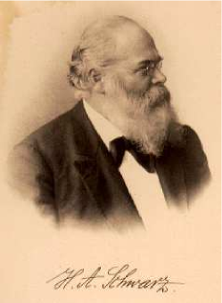
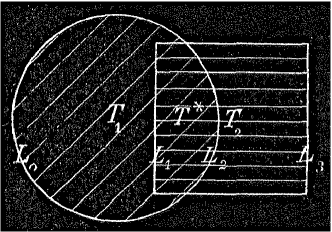
Figure 1.1: Left: Herman Amandus Schwarz (25.1.1843-30.11.1921). Right: original figure for the decomposition in the alternating Schwarz method.

Schwarz invented the now called alternating Schwarz method in order to close a gap in the proof of the Riemann mapping theorem at the end of Riemann’s PhD thesis (?), an English translation of which is available (?). In his proof, Riemann had assumed that the Dirichlet problem

$$\Delta u=0\ \mbox{in $\Omega$},\quad\hbox{$u=g$ on $\partial\Omega$},$$ (1)

always had a solution, just by taking the function $u(x,y)$ which solves the minimization problem

$${\cal J}(u):=\iint_{\Omega}\bigl{(}\frac{\partial u}{\partial x}\bigr{)}^{2}+\bigl{(}\frac{\partial u}{\partial y}\bigr{)}^{2}\D x\D y\longrightarrow\min,\quad\hbox{$u=g$ on $\partial\Omega$},$$ (2)

and satisfies the boundary condition $u=g$ on $\partial\Omega$. When asked why this minimization problem had always a solution, Riemann replied that he had learned this in his analysis course taught by Dirichlet, the functional ${\cal J}(u)$ being bounded from below, thus coining the term Dirichlet principle. ? then presented a counterexample to this way of arguing: the functional to minimize, $\int_{-1}^{+1}(x\cdot u^{\prime})^{2}\D x\longrightarrow\min$, is also bounded from below, but when one tries to find a function that minimizes this integral with boundary conditions $u(-1)=a$, $u(1)=b$, $a\neq b$, $u^{\prime}$ should be small when $x$ is away from zero, best is taking $u^{\prime}=0$ so there is no contribution to the integral, and when $x=0$, $u^{\prime}$ can be large, since it is multiplied with $0$ and thus also does not contribute. The minimizing “solution” is thus piecewise constant and discontinuous at $x=0$, and the gap in Riemann’s proof remained. However, the Dirichlet problem eq:DirichletProblem had a well known solution on rectangular and circular domains, using Fourier techniques from 1822. H.A. Schwarz invented his alternating method by choosing as domain $\Omega$ the union of a disk and an overlapping rectangle (see Figure 1.1 (right)). If we call the overlapping subdomains $\Omega_{1}$ and $\Omega_{2}$ ($T_{1}$ and $T_{2}$ in the original drawing of Schwarz), and the interfaces $\Gamma_{1}$ and $\Gamma_{2}$ ($L_{2}$ and $L_{1}$ in the original drawing of Schwarz), the alternating Schwarz method computes alternatingly on the disk and on the rectangle the Dirichlet problem and carries the newly computed solution from the interface curves $\Gamma_{1}$ and $\Gamma_{2}$ over to the other subdomain as new boundary condition for the next solve,

$$\begin{array}[]{rcllrcll}\Delta u_{1}^{n}&=&0&\mbox{in $\Omega_{1}$},&\Delta u_{2}^{n}&=&0&\mbox{in $\Omega_{2}$},\\ u_{1}^{n}&=&g&\mbox{on $\partial\Omega\cap\overline{\Omega}_{1}$},&u_{2}^{n}&=&g&\mbox{on $\partial\Omega\cap\overline{\Omega}_{2}$},\\ u_{1}^{n}&=&u_{2}^{n-1}&\mbox{on $\Gamma_{1}$},&u_{2}^{n}&=&u_{1}^{n}&\mbox{on $\Gamma_{2}$}.\end{array}$$ (3)

Schwarz proved convergence of this alternating method using the maximum principle, see ? for more information on the origins of the alternating Schwarz method. All this happened during the fascinating time of the development of variational calculus and functional analysis, which led eventually to the finite element method, see the historical review ?.

It took many decades before the alternating Schwarz method became a computational tool. ? was the first to point out its usefulness for computations, but it was with the seminal work of Lions (?, ?, ?), and the additive Schwarz method of ?, that Schwarz methods became powerful and mainstream parallel computational tools for solving discretized partial differential equations. ? also proposed a parallel variant of the method, by simply not using the newest available value along $\Gamma_{2}$ but the previous one in AlternatingSchwarzMethod,

$$u_{2}^{n}=u_{1}^{n-1}\ \mbox{on $\Gamma_{2}$},$$ (4)

so that the subdomain solves can be performed in parallel. This is analogous to the Jacobi stationary iterative method, compared to the Gauss-Seidel stationary iterative method in linear algebra. Note that the additive Schwarz method is quite different from the parallel Schwarz method: it is a preconditioner for the conjugate gradient method, and does not converge when used as a stationary iteration without relaxation, in contrast to the parallel Schwarz method, see ? for more details.

? also introduced a non-overlapping variant of the Schwarz method using Robin transmission conditions in AlternatingSchwarzMethod,

$$\begin{array}[]{rcllrcll}(\partial_{n_{1}}\!+\!p_{1})u_{1}^{n}&=&(\partial_{n_{1}}\!+\!p_{1})u_{2}^{n-1}&\mbox{on $\Gamma_{1}$},&(\partial_{n_{2}}\!+\!p_{2})u_{2}^{n}&=&(\partial_{n_{2}}\!+\!p_{2})u_{1}^{n}&\mbox{on $\Gamma_{2}$},\end{array}$$

where $\partial_{n_{j}}$, $j=1,2$, denotes the unit outward normal derivative for $\Omega_{j}$ along the interfaces $\Gamma_{j}$, and, following Lions, the $p_{j}$ can be constants, or functions along the interface, or even operators. In contrast to the classical Schwarz method, where it was only important to obtain convergence for closing the gap in the proof of the Riemann mapping theorem, and convergence speed was not an issue, a good choice of the Robin parameters $p_{j}$ can greatly improve the convergence of Schwarz methods. ? worked on Schwarz methods for non-linear problems, and advocated to use Robin transmission conditions involving non-local operators. The work of ? on generalized Schwarz splittings also points into this direction, for a more detailed review, see ?.

What is the underlying idea of changing the transmission conditions from Dirichlet to Robin conditions, even involving non-local operators? In Schwarz methods for parallel computing, one decomposes a domain into many subdomains, see Figure 1.2 for two typical examples.

Figure 1.2: Two typical domain decompositions: a two dimensional decomposition with cross points (left), and a one dimensional or sequential domain decomposition (right).

To obtain an overlapping decomposition, it is convenient to first define a decomposition into non-overlapping subdomains $\tilde{\Omega}_{ij}$, and then to enlarge these subdomains by a thin layer to get overlapping subdomains $\Omega_{ij}$, as indicated in Figure 1.2. One then wants to compute only subdomain solutions on the $\Omega_{ij}$ to approximate the global, so called mono-domain solution on the entire domain $\Omega$. Let us imagine for the moment that the source term of the partial differential equation to be solved has only support in one subdomain somewhere in the middle of the global domain, like for example in subdomain $\Omega_{ij}$ in Figure 1.2 on the left, and assume that the global domain is infinitely large. Then it would be best to put on the boundary of the subdomain containing the source transparent boundary conditions, since then by solving the subdomain problem we obtain by definition the restriction of the global, mono-domain solution to that subdomain. Robin boundary conditions are approximations of the transparent boundary conditions, and one can thus expect that with Robin boundary conditions subdomain solvers compute better approximations to the overall mono-domain solution than with Dirichlet boundary conditions.

To illustrate this, we solve the Poisson problem $\Delta u=f$ on the unit square with zero Dirichlet boundary conditions and the right hand side source function $f(x,y):=100e^{-100((x-\frac{1}{2})^{2}+(y-\frac{1}{2})^{2})}$. We show in Figure 1.3 on the left this source term, and on the right the corresponding solution of the Poisson problem, using a centered finite difference scheme with mesh size $h=1/40$.

 

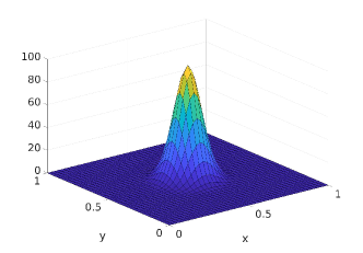
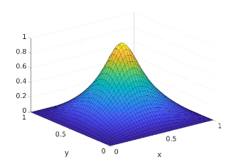
Figure 1.3: Gaussian source term (left) and solution on of the corresponding Poisson problem (right).

If we decompose the unit square domain into $3\times 3$ subdomains as indicated in Figure 1.2 (left), and solve the subdomain problem in the center with Dirichlet boundary conditions $u=0$, we obtain the approximation shown in Figure 1.4 (top left).

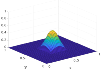
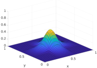
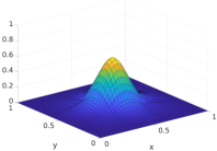
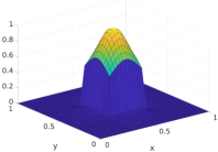
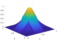
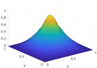
Figure 1.4: First few iterations of classical (top) and optimized parallel Schwarz (bottom) for the Poisson problem with Gaussian source term from Figure 1.3.

If we perform the solve with Robin conditions $(\partial_{n}+p)u=0$ with $p=4$, we get the approximation shown in Figure 1.4 (bottom left). We clearly see that the result when truncating with Dirichlet conditions is much further away from the desired solution shown in Figure 1.3 (right) than when truncating with Robin conditions. This is however precisely the first iteration of a classical Schwarz method with Dirichlet transmission conditions, compared to an optimized Schwarz method with Robin transmission conditions, when starting the iteration with a zero initial guess. We show in Figure 1.4 also the next two iterations of the classical (top) and optimized Schwarz method (bottom) with algebraic overlap of two mesh layers, and we see the great convergence enhancement due to the Robin transmission conditions, which are much better approximations of the transparent boundary conditions than the Dirichlet transmission conditions. This illustrates well that Schwarz methods (and domain decomposition methods in general) are methods which approximate solutions by domain truncation, and we see that transmission conditions that are better at truncating domains lead to better convergence.

This became a major new viewpoint on domain decomposition methods over the past two decades. Naturally Dirichlet (and Neumann) conditions then appear as not very good candidates to truncate domains and be used as transmission conditions between subdomains: it is of interest for rapid convergence to use absorbing boundary conditions which approximate transparent conditions, like Robin conditions or higher order Ventcell conditions, and also perfectly matched layers (PMLs), or integral operators in the transmission conditions between subdomains.

Optimized Schwarz methods were pioneered in the early nineties by Nataf et al. (?, ?); see in particular also the early contributions of ?, ?, ?, and ? where the name optimized Schwarz methods was coined. Optimized Schwarz methods use Robin or higher order transmission conditions or PMLs at the interfaces between subdomains, and all are approximations of transparent boundary conditions, see ? and references therein for an introduction. This conceptual change for domain decomposition methods is fundamental and was discovered independently for solving hard wave propagation problems by domain decomposition and iteration, since for such problems classical domain decomposition methods are not effective, see the seminal work by ?, ?, and ? for a review why it is hard to solve such problems by iteration. Also rational approximations have been proposed in the transmission conditions for such problems, see for example ?, ?, ?. This new idea of domain truncation led, independently of the work on optimized Schwarz methods, to the invention of the sweeping preconditioner (?, ?, ?, ?, ?, ?), the source transfer domain decomposition (?, ?, ?), the single layer potential method (?, ?), and the method of polarized traces (?, ?, ?). All these methods are very much related, and can be understood in the context of optimized Schwarz methods, for a review and formal proofs of equivalence, see ?, and also the references therein for the many followup papers by the various groups. A key ingredient of these independently developed methods is the use of perfectly matched layers as absorbing boundary conditions, a technique which had only rarely been used in the domain decomposition community before, for exceptions see ?, ?, ?.

While optimized Schwarz methods were developed for general decompositions of the domain into subdomains, including cross points, as shown on the left in Figure 1.2 and in the corresponding example in Figure 1.4, the sweeping preconditioner, source transfer domain decomposition, the single layer potential method and the method of polarized traces were all formulated for one dimensional or sequential domain decompositions, as shown in Figure 1.2 on the right, without cross points. This is because these methods were developed with the physical intuition of wave propagation in one direction, and not with domain decomposition in mind. In these methods, the authors had in mind the transparent boundary conditions at the interfaces, which contain the Dirichlet to Neumann (DtN), or more generally the Steklov Poincaré operator replacing $p$ in the Robin transmission condition, and with this choice, the method becomes a direct solver. We illustrate this in Figure 1.5 for the strip decomposition in Figure 1.2 (right) with three subdomains and our Poisson model problem with Gaussian source from Figure 1.3.

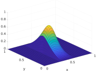
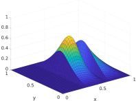
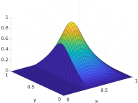
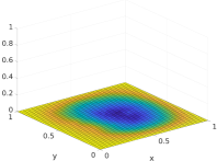
Figure 1.5: Optimal alternating Schwarz using DtN transmission conditions sweeping with the iterates from left to right and then back to left (double sweep) for a sequential decomposition into three subdomains, solving the Poisson problem with Gaussian source term from Figure 1.3. The last figure shows the error after one double sweep, on the order of machine precision.

We see that the method converges in one double sweep, i.e. it is a direct solver. The iteration matrix (or operator at the continuous level) is nilpotent, and one can interpret this method as an exact block LU factorization, where in the forward sweep the lower block triangular matrix $L$ is solved, and in the backward sweep the upper block triangular matrix $U$ is solved, and the blocks correspond to the subdomains. This interpretation had already led earlier to the Analytic Incomplete LU (AILU) preconditioners, see ?, ? and references therein. Note that other domain decomposition methods can also be nilpotent for sequential domain decompositions: for Neumann-Neumann and FETI this is however only possible for two-subdomain decompositions, and for Dirichlet-Neumann up to three subdomains, and in some specific cases more than three subdomains, see ?. The only domain decomposition method which can in general become nilpotent for sequential domain decompositions is the optimal Schwarz method.

If we use approximations of the optimal Schwarz method, for example an optimized one with Robin transmission conditions, the method is not nilpotent any more, as shown in Figure 1.6,

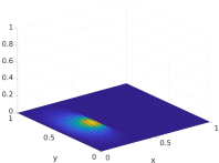
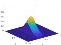
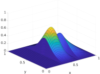
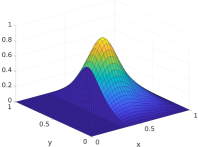
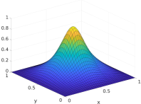
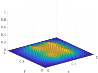
Figure 1.6: Optimized alternating Schwarz using Robin transmission conditions sweeping like optimal alternating Schwarz in Figure 1.5 (the last figure shows the error after one double sweep).

but convergence is still very fast, compared to the classical Schwarz method with Dirichlet transmission conditions shown in Figure 1.7.

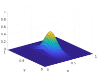
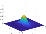
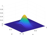
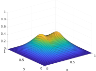
Figure 1.7: Classical alternating Schwarz (using Dirichlet transmission conditions) sweeping like optimized alternating Schwarz in Figure 1.6 (the last figure shows the error after one double sweep).

Using PML as transmission conditions in optimized Schwarz methods to approximate the optimal DtN transmission conditions is currently a very active field of research in the case of cross points. ? proposed a parallel Schwarz method for checkerboard domain decompositions including cross points based on the source transfer formalism which uses PML transmission conditions, and the method still converges in a finite number of steps, see also ? for a diagonal sweeping variant, and the earlier work (?, ?). In ?, L-sweeps are proposed for the method of polarized traces interpretation of the optimized Schwarz methods, which traverse a square domain decomposed into little squares by subdomain solves organized in the form of L’s, from one corner going over the domain. In these methods, storing the PML layers and using them in the exchange of information is an essential ingredient, and it is not clear at this stage if such a formulation using DtN transmission conditions is possible.

It is however possible to use the block LU decomposition also in the case of general decompositions including cross points, to obtain a sweeping domain decomposition method which converges in one double sweep. We show this in Figure 1.8

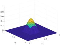
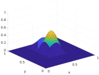
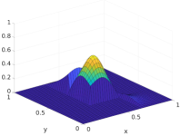
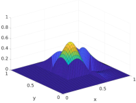
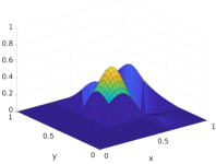
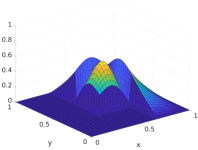
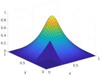
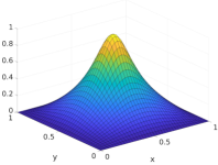
Figure 1.8: Forward and backward sweep for an optimal Schwarz method obtained by a block LU decomposition for the model problem and $3\times 3$ subdomains. We observe convergence after one double sweep.

for our model problem and the same $3\times 3$ domain decomposition used in Figure 1.4. We have chosen here simply a lexicographic ordering of the subdomains, and we see that the method converges in one double sweep. We show in Figure 1.9

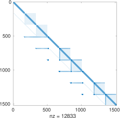
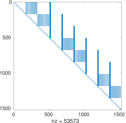
Figure 1.9: Sparsity of the block $L$ and $U$ factors of the optimal Schwarz method for the $3\times 3$ subdomain decomposition from Figure 1.8.

the sparsity structure of the corresponding LU factors, which indicate the structure of the transmission conditions generated by the block LU decomposition in this case, a subject that needs further investigation; if the domain decomposition is a strip decomposition without cross points, i.e. like in Figure 1.2 on the right, it is known that the block LU decomposition generates transparent transmission conditions on the left and Dirichlet conditions on the right of the subdomains, like in the design of the source transfer domain decomposition method. There is uniqueness in the block LU decomposition only once one chooses the diagonal of one of the factors, e.g. the identity matrices on the diagonal of $U$ as we did here. For the strip decomposition our block LU factorization gives therefore a different algorithm from the optimal Schwarz method shown in Figure 1.5 which used transparent boundary conditions involving the DtN operator on both sides of the subdomains. We give a simple Matlab implementation for these block LU factorizations in Appendix A for the interested reader to experiment with.

Note that we could have used any other ordering of the subdomains for the sweeping before performing the block LU factorization: we show for example in Figure 1.10

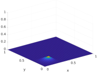
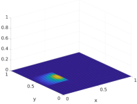
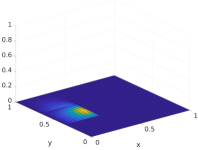
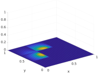
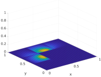
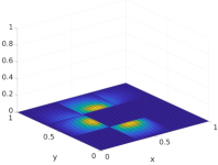
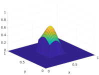
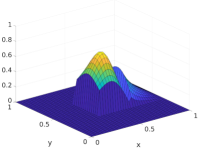
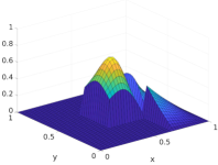
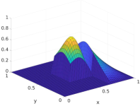
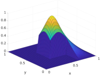
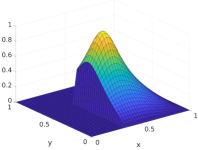
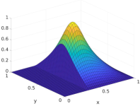
Figure 1.10: Forward and backward sweep for an optimal Schwarz method obtained by a block LU decomposition for the model problem and $3\times 3$ subdomains using an L-sweep. We observe again convergence after one double sweep.

the ordering for L-sweeps. We see that the algorithm also converges in one double sweep, by construction. The corresponding block LU factors are shown in Figure 1.11.

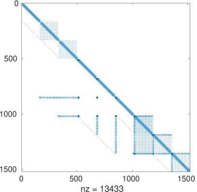
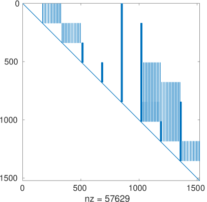
Figure 1.11: Sparsity of the block $L$ and $U$ factors of the optimal Schwarz method for the $3\times 3$ subdomain decomposition from Figure 1.8 when using the L-sweep ordering.

We show in Figure 1.12 the further popular diagonal ordering for sweeping.

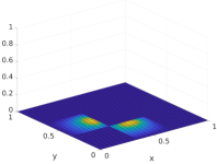
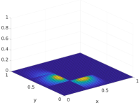
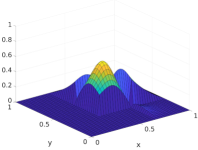
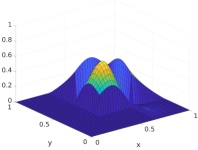
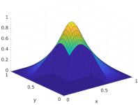
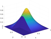
Figure 1.12: Forward and backward sweep for an optimal Schwarz method obtained by a block LU decomposition for the model problem and $3\times 3$ subdomains using a D-sweep. We observe again convergence after one double sweep.

Again we see convergence in one double sweep. The corresponding block LU factors are shown in Figure 1.13.

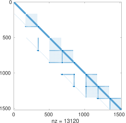
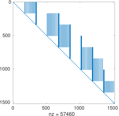
Figure 1.13: Sparsity of the block $L$ and $U$ factors of the optimal Schwarz method for the $3\times 3$ subdomain decomposition from Figure 1.8 when using the D-sweep ordering.

It is currently not known how to obtain a general parallel nilpotent Schwarz method for such general decompositions including cross points. It was however discovered in ? that it is possible to define transmission conditions at the algebraic level, including a global communication component, such that the associated optimal parallel Schwarz method converges in two (!) iterations, independently of the number of subdomains, the decomposition and the partial differential equation that is solved. Such a global communication component is also present in the recent work (?, ?) for time harmonic wave propagation problems, which is based on earlier work of ?, where the multi-trace formulation was interpreted as an optimized Schwarz method, including cross points.

We will use in what follows the two specific domain decompositions shown in Figure 1.2, namely one dimensional, sequential or strip decompositions, and two dimensional decompositions including cross points. For sequential domain decompositions, we can use Fourier analysis techniques to accurately study the influence of the transmission conditions used on the convergence of the domain decomposition iteration, whereas for two dimensional domain decompositions, such results are not yet available.

2 Two subdomain analysis

It is very instructive to understand Schwarz methods by domain truncation starting first with a simple two subdomain decomposition, since then many detailed convergence properties of the Schwarz methods can be obtained by direct, analytical computations. We consider therefore the strip decomposition shown in Figure 1.2 on the right but with only two subdomains, $\Omega_{1}:=(0,X_{1}^{r})\times(0,Y)$ and $\Omega_{2}:=(X_{2}^{l},1)\times(0,Y)$. Throughout the paper, by $y=O(x)$ we mean $C_{1}|x|\leq|y|\leq C_{2}|x|$ for some constant $C_{1},C_{2}>0$ independent of $x$, and we write the asymptotic $y\sim x$ if $\lim y/x=1$ and $x$ consists of the leading terms.

2.1 Laplace type problems

We study first the screened Laplace equation (sometimes also called the Helmholtz equation with the “good sign”),

$$(\eta-\Delta)u=f\quad\mbox{in $\Omega:=(0,1)\times(0,Y)$},$$ (5)

with $\eta\geq 0$. As boundary conditions, we impose on the left and right a Robin boundary condition,

$${\cal B}^{l}(u):=\partial_{n}u+p^{l}u=g^{l},\quad{\cal B}^{r}(u):=\partial_{n}u+p^{r}u=g^{r},$$ (6)

where $\partial_{n}$ denotes the unit outer normal derivative (i.e. $-\partial_{x}$ on the left and $\partial_{x}$ on the right). On top and bottom we impose either a Dirichlet or a Neumann condition,

$$\begin{array}[]{rcll}{\cal B}^{b}(u)&=&g^{b}&\mbox{with either ${\cal B}^{b}(u):=u$ or ${\cal B}^{b}(u):=\partial_{n}u$},\\ {\cal B}^{t}(u)&=&g^{t}&\mbox{with either ${\cal B}^{t}(u):=u$ or ${\cal B}^{t}(u):=\partial_{n}u$}.\end{array}$$ (7)

An alternating Schwarz method then starts with an initial guess $u_{2}^{0}$ in subdomain $\Omega_{2}$ and performs for iteration index $n=1,2,\ldots$ alternatingly solutions on the subdomains,

$$\begin{array}[]{rcllrcll}(\eta-\Delta)u_{1}^{n}&=&f&\mbox{in $\Omega_{1}$},&(\eta-\Delta)u_{2}^{n}&=&f&\mbox{in $\Omega_{2}$},\\ {\cal B}_{1}^{r}(u_{1}^{n})&=&{\cal B}_{1}^{r}(u_{2}^{n-1})&\mbox{at $x=X_{1}^{r}$},&{\cal B}_{2}^{l}(u_{2}^{n})&=&{\cal B}_{2}^{l}(u_{1}^{n})&\mbox{at $x=X_{2}^{l}$},\\ {\cal B}^{l}(u_{1}^{n})&=&g^{l}&\mbox{at $x=0$},&{\cal B}^{r}(u_{2}^{n})&=&g^{r}&\mbox{at $x=1$},\\ {\cal B}^{b}(u_{1}^{n})&=&g^{b}&\mbox{at $y=0$},&{\cal B}^{b}(u_{2}^{n})&=&g^{b}&\mbox{at $y=0$},\\ {\cal B}^{t}(u_{1}^{n})&=&g^{t}&\mbox{at $y=Y$},&{\cal B}^{t}(u_{2}^{n})&=&g^{t}&\mbox{at $y=Y$}.\end{array}$$ (8)

Here the key ingredient are the transmission conditions ${\cal B}_{1}^{r}$ and ${\cal B}_{2}^{l}$, which in the classical Schwarz method are Dirichlet, see AlternatingSchwarzMethod, but in Schwarz methods based on domain truncation, e.g. optimized Schwarz methods, they are of the form

$${\cal B}_{1}^{r}(u):=\partial_{n}u+{\cal S}_{1}^{r}(u),\quad{\cal B}_{2}^{l}(u):=\partial_{n}u+{\cal S}_{2}^{l}(u).$$ (9)

Here ${\cal S}_{1}^{r}$ and ${\cal S}_{2}^{l}$ can either be constants, ${\cal S}_{1}^{r}=p_{1}$, ${\cal S}_{2}^{l}=p_{2}$, $p_{j}\in\mathbb{R}$, which leads to Robin transmission conditions, or more general tangential operators acting along the interface, e.g. ${\cal S}_{1}^{r}=p_{1}-q_{1}\partial_{yy}$ with $p_{1},q_{1}\in\mathbb{R}$, which would be Ventcell transmission conditions, or one can also consider more general transmission conditions involving rational functions or PMLs, see ? and references therein.

In order to study the convergence of the Schwarz method SMDT, we introduce the error $e_{j}^{n}:=u-u_{j}^{n}$, $j=1,2$, which by linearity satisfies the same iteration equations as the original algorithm, but with zero data, i.e.

$$\begin{array}[]{rcllrcll}(\eta-\Delta)e_{1}^{n}&=&0&\mbox{in $\Omega_{1}$},&(\eta-\Delta)e_{2}^{n}&=&0&\mbox{in $\Omega_{2}$},\\ {\cal B}_{1}^{r}(e_{1}^{n})&=&{\cal B}_{1}^{r}(e_{2}^{n-1})&\mbox{at $x=X_{1}^{r}$},&{\cal B}_{2}^{l}(e_{2}^{n})&=&{\cal B}_{2}^{l}(e_{1}^{n})&\mbox{at $x=X_{2}^{l}$},\\ {\cal B}^{l}(e_{1}^{n})&=&0&\mbox{at $x=0$},&{\cal B}^{r}(e_{2}^{n})&=&0&\mbox{at $x=1$},\\ {\cal B}^{b}(e_{1}^{n})&=&0&\mbox{at $y=0$},&{\cal B}^{b}(e_{2}^{n})&=&0&\mbox{at $y=0$},\\ {\cal B}^{t}(e_{1}^{n})&=&0&\mbox{at $y=Y$},&{\cal B}^{t}(e_{2}^{n})&=&0&\mbox{at $y=Y$},\end{array}$$ (10)

as one can easily verify by directly evaluating the expressions on the left of the equal signs, e.g.

$$(\eta-\Delta)e_{1}^{n}=(\eta-\Delta)(u-u_{1}^{n})=f-f=0.$$

To obtain detailed information on the functioning of such Schwarz methods, it is best to expand the errors in a Fourier series in the $y$ direction,

$$e_{j}^{n}=\sum_{\tilde{k}=0}^{\infty}\hat{e}_{j}^{n}(\tilde{k})\cos(\frac{\tilde{k}\pi}{Y}y)+\sum_{\tilde{k}=1}^{\infty}\hat{\epsilon}_{j}^{n}(\tilde{k})\sin(\frac{\tilde{k}\pi}{Y}y).$$ (11)

Now if at the bottom and top we have Dirichlet conditions, all the error coefficients of the cosine are zero, and if we have Neumann conditions, all the error coefficients of the sine are zero. In either case, inserting the Fourier series into the error equations SMDTerror, we obtain by orthogonality of the sine and cosine functions for each cosine error Fourier mode $\hat{e}_{j}^{n}$, $j=1,2$ (and analogously for the sine error Fourier mode $\hat{\epsilon}_{j}^{n}$) the Schwarz iteration

$$(\eta-\partial_{xx}+k^{2})\hat{e}_{1}^{n} =0 \mbox{in $(0,X_{1}^{r})$}, (\eta-\partial_{xx}+k^{2})\hat{e}_{2}^{n} =0 \mbox{in $(X_{2}^{l},1)$},$$ (12)

$$\beta_{1}^{r}(\hat{e}_{1}^{n}) =\beta_{1}^{r}(\hat{e}_{2}^{n-1}) \mbox{at $x=X_{1}^{r}$}, \beta_{2}^{l}(\hat{e}_{2}^{n}) =\beta_{2}^{l}(\hat{e}_{1}^{n}) \mbox{at $x=X_{2}^{l}$},$$

$$\beta^{l}(\hat{e}_{1}^{n}) =0 \mbox{at $x=0$}, \beta^{r}(\hat{e}_{2}^{n}) =0 \mbox{at $x=1$},$$

where we defined the frequency variable $k:=\frac{\tilde{k}\pi}{Y}$, and $\beta_{1}^{r}$, $\beta_{2}^{l}$, $\beta^{l}$, $\beta^{r}$ denote the Fourier transforms of the boundary operators, also called their symbols, e.g. $\beta_{1}^{r}=\partial_{n}+\sigma_{1}^{r}$ with $\sigma_{1}^{r}$ the symbol of the tangential operator chosen in TC. If this operator was for example ${\cal S}_{1}^{r}=p_{1}-q_{1}\partial_{yy}$, $p_{1}$, $q_{1}$ constants, then its symbol would be $\sigma_{1}^{r}=p_{1}+q_{1}k^{2}$, from the two derivatives acting on the cosine, which also leads to the sign change from minus to plus.

Solving the ordinary differential equations in the error iteration SMDTerrorF, we obtain using the outer Robin boundary conditions for each Fourier mode $k$ the solutions (with $\underline{x}:=1-x$)

$$\hat{e}_{1}^{n}(x,k) =A_{1}^{n}(k)\left({\sqrt{k^{2}+\eta}\cosh(\sqrt{k^{2}+\eta}x)+p^{l}\sinh(\sqrt{k^{2}+\eta}x)}\right),$$ (13)

$$\hat{e}_{2}^{n}(x,k) =A_{2}^{n}(k)\left({\sqrt{k^{2}+\eta}\cosh(\sqrt{k^{2}+\eta}\underline{x})+p^{r}\sinh(\sqrt{k^{2}+\eta}\underline{x})}\right).$$

To determine the two remaining constants $A_{1}^{n}(k)$ and $A_{2}^{n}(k)$ we insert the solutions into the transmission conditions in SMDTerrorF, which leads to

$$A_{1}^{n}=\rho_{1}(k,\eta,p^{l},p^{r},\sigma_{1}^{r})A_{2}^{n-1},\quad A_{2}^{n}=\rho_{2}(k,\eta,p^{l},p^{r},\sigma_{2}^{l})A_{1}^{n},$$ (14)

with the two quantities

$$\begin{array}[]{rcl}\rho_{1}&=&\frac{(k^{2}-\sigma_{1}^{r}p^{r}+\eta)\sinh(\sqrt{k^{2}+\eta}(X_{1}^{r}-1))-\cosh(\sqrt{k^{2}+\eta}(X_{1}^{r}-1))\sqrt{k^{2}+\eta}(p^{r}-\sigma_{1}^{r})}{(k^{2}+\sigma_{1}^{r}p^{l}+\eta)\sinh(\sqrt{k^{2}+\eta}X_{1}^{r})+\cosh(\sqrt{k^{2}+\eta}X_{1}^{r})\sqrt{k^{2}+\eta}(p^{l}+\sigma_{1}^{r})},\\ \rho_{2}&=&\frac{(k^{2}-\sigma_{2}^{l}p^{l}+\eta)\sinh(\sqrt{k^{2}+\eta}X_{2}^{l})+\cosh(\sqrt{k^{2}+\eta}X_{2}^{l})\sqrt{k^{2}+\eta}(p^{l}-\sigma_{2}^{l})}{(k^{2}+\sigma_{2}^{l}p^{r}+\eta)\sinh(\sqrt{k^{2}+\eta}(X_{2}^{l}-1))-\cosh(\sqrt{k^{2}+\eta}(X_{2}^{l}-1))\sqrt{k^{2}+\eta}(p^{r}+\sigma_{2}^{l})}.\end{array}$$ (15)

Their product represents the convergence factor of the Schwarz method,

$$\rho(k,\eta,p^{l},p^{r},\sigma_{1}^{r},\sigma_{2}^{l}):=\rho_{1}(k,\eta,p^{l},p^{r},\sigma_{1}^{r})\rho_{2}(k,\eta,p^{l},p^{r},\sigma_{2}^{l}),$$ (16)

i.e. it determines by which coefficient the corresponding error Fourier mode $k$ is multiplied over each alternating Schwarz iteration.

Since the expression for the convergence factor $\rho$ looks rather complicated, it is instructive to look at the special case first where the domain, and thus the subdomains, are unbounded on the left and right. This can be obtained from the result above by introducing for the outer boundary conditions a transparent one, i.e. choosing for the Robin parameters the symbol of the DtN operator $p^{r}:=\sqrt{k^{2}+\eta}$, $p^{l}:=\sqrt{k^{2}+\eta}$. This leads after simplification to the convergence factor

$$\rho(k,\eta,\sigma_{1}^{r},\sigma_{2}^{l})=\frac{\sqrt{k^{2}+\eta}-\sigma_{1}^{r}}{\sqrt{k^{2}+\eta}+\sigma_{1}^{r}}\frac{\sqrt{k^{2}+\eta}-\sigma_{2}^{l}}{\sqrt{k^{2}+\eta}+\sigma_{2}^{l}}e^{-2(X_{1}^{r}-X_{2}^{l})\sqrt{k^{2}+\eta}}.$$ (17)

This convergence factor shows us a very important property of these Schwarz methods: if we choose $\sigma_{1}^{r}=\sigma_{2}^{l}:=\sqrt{k^{2}+\eta}$, the tangential symbol of the transparent boundary condition, the convergence factor vanishes identically for all Fourier frequencies $k$, i.e. after two consecutive subdomain solves, one on the left and one on the right (or vice versa), the error in each Fourier mode is zero, i.e. we have the exact solution on the subdomain after two alternating subdomain solves! This is called an optimal Schwarz method, see footnote 5. If we thus used a double sweep, first solving on the left subdomain and then on the right, followed by another solve on the left (or a double sweep in the other direction), we would have the solution on both subdomains, which shows for two subdomains the double sweep result illustrated in Figure 1.5 for three subdomains. This result holds in general for many subdomains in the strip decomposition case; it was first proved in ? for an advection diffusion problem. If we use the parallel Schwarz method for two subdomains, then we need two iterations in order to have each subdomain solved one after the other, so the optimal parallel Schwarz method for two subdomains will converge in two iterations, a result that generalizes to convergence in $J$ iterations for $J$ subdomains in the strip decomposition case, first proved in ?.

In the bounded domain case, we can still obtain these same results by chosing in the transmission conditions the tangential symbols of the transparent boundary conditions for the bounded subdomains, which is equivalent to choosing $\sigma_{1}^{r}$ and $\sigma_{2}^{l}$ such that $\rho_{1}$ and $\rho_{2}$ in rho12 vanish, which leads to

$$\begin{array}[]{rcl}\sigma_{1}^{r}&=&\frac{\sqrt{k^{2}+\eta}\left(\tanh(\sqrt{k^{2}+\eta}(X_{1}^{r}-1))\sqrt{k^{2}+\eta}-p^{r}\right)}{\tanh(\sqrt{k^{2}+\eta}(X_{1}^{r}-1))p^{r}-\sqrt{k^{2}+\eta}},\\ \sigma_{2}^{l}&=&\frac{\sqrt{k^{2}+\eta}\left(\tanh(\sqrt{k^{2}+\eta}X_{2}^{l})\sqrt{k^{2}+\eta}+p^{l}\right)}{\tanh(\sqrt{k^{2}+\eta}X_{2}^{l})p^{l}+\sqrt{k^{2}+\eta}}.\end{array}$$ (18)

As in the unbounded domain case, these values correspond to the symbols of the associated DtN operators on the bounded domain, as one can verify by a direct computation using the solutions ScreenedLaplaceSols on their respective domains, as done for the unbounded domain in footnote 8. We see that in the bounded domain case, the symbols of the DtN maps in DtNbdd, and hence the DtN maps also, depend on the outer boundary conditions, since both the domain parameters ($X_{1}^{r}$ and $X_{2}^{l}$) and the Robin parameters in the outer boundary conditions ($p^{l}$ and $p^{r}$) appear in them. However, for large frequencies $k$, we have

$$\sigma_{1}^{r}\sim\sqrt{k^{2}+\eta},\quad\sigma_{2}^{l}\sim\sqrt{k^{2}+\eta},$$

since $\tanh z\to\pm 1$ as $z\to\pm\infty$, and thus only low frequencies see the difference from the bounded to the unbounded case in the screened Laplace problem.

Choosing Robin transmission conditions, ${\cal S}_{1}^{r}:=p_{1}^{r}=\sigma_{1}^{r}$ and ${\cal S}_{2}^{l}:=p_{2}^{l}=\sigma_{2}^{l}$ with $p_{1}^{r},p_{2}^{l}\in\mathbb{R}$ in TC, and taking the limit in the convergence factor RhoOSMUnbounded as the Robin parameters $p_{1}^{r}$ and $p_{2}^{l}$ go to infinity, we find

$$\rho(k,\eta,)=e^{-2(X_{1}^{r}-X_{2}^{l})\sqrt{k^{2}+\eta}},$$ (19)

which is the convergence factor of the classical alternating Schwarz method on the unbounded domain, since the transmission conditions TC become Dirichlet transmission conditions in this limit of the Robin transmission conditions. We see now explicitly the overlap $L:=X_{1}^{r}-X_{2}^{l}$ appearing in the exponential function. The classical Schwarz method for the screened Laplace problem therefore converges for all Fourier modes $k$, provided there is overlap, and $\eta>0$. If $\eta=0$, i.e. we consider the Laplace problem, then the Fourier mode $k=0$ does not contract on the unbounded domain. Recall however that $k=0$ is only present in the cosine expansion for Neumann boundary conditions on top and bottom, it is the constant mode, and the Schwarz method on the unbounded domain does indeed not contract for this mode. For Dirichlet boundary conditions on top and bottom, i.e. considering the sine series in (11), the smallest Fourier frequency is $k=\frac{\pi}{Y}>0$ so the Schwarz method is contracting, even with $\eta=0$. Note also that the contraction is faster for large Fourier frequencies $k$ than for small ones due to the exponential function, and hence the Schwarz method is a smoother for the screened Laplace equation. A comparison of the classical Schwarz convergence factor RhoAltSUnbounded with the convergence factor for the optimized Schwarz method with Robin transmission conditions in RhoOSMUnbounded shows that the latter contains the former, but in addition also the two fractions in front which are also smaller than one for suitable choices of the Robin parameters. The optimized Schwarz method therefore always converges faster than the classical Schwarz method, and furthermore can also converge without overlap, which was the original reason for Lions to propose Robin transmission conditions.

To see how the classical Schwarz method contracts on a bounded domain, we show in Figure 2.1 (left) the different cases for the outer boundary conditions ($p^{l}=p^{r}=5$ in the Robin case), by plotting RhoOSM for when the parameters in the Robin transmission conditions go to infinity, and the model parameter $\eta=1$, for a small overlap, $L=X_{1}^{r}-X_{2}^{l}=0.51-0.49=0.02$.

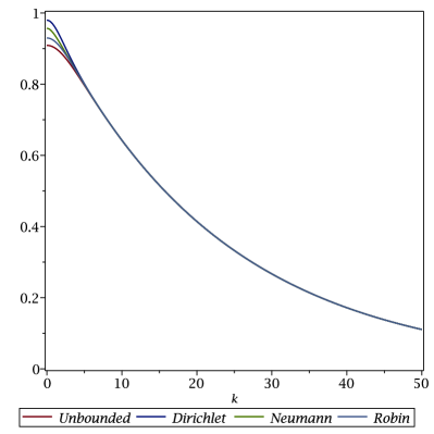
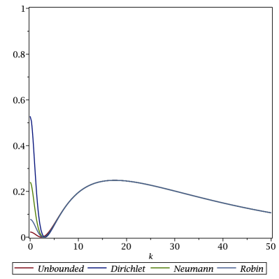
Figure 2.1: Left: classical Schwarz convergence factor for $\eta-\Delta$ and different outer boundary conditions on the left and right. Right: corresponding Schwarz convergence factor with Robin transmission conditions.

This shows that the different outer boundary conditions only influence the convergence of the lowest frequencies ($k$ small) in the error, for larger frequencies there is no influence. This is due to the diffusive nature of the screened Laplace equation: high freqency components are damped rapidly by the (screened) Laplace operator, and thus they don’t see the different outer boundary conditions. On the right in Figure 2.1 we show the corresponding convergence factors with Robin transmission conditions, chosen as $p_{1}^{r}=p_{2}^{l}=3$. This indicates that there is an optimal choice which leads to the fastest possible convergence, which in our example is achieved for the Neumann outer boundary condition with the choice $p_{1}^{r}=p_{2}^{l}\approx 3$, since the maximum of the convergence factor is minimized by equioscillation, i.e. the convergence factor at $k=0$ equals the convergence factor at the interior maximum at around $k=18$. For different outer boundary conditions, there would be a better value of $p_{1}^{r}=p_{2}^{l}$ that makes e.g.  the blue curve for Dirichlet outer boundary conditions equioscillating. This optimization process led to the name optimized Schwarz methods.

Let us compute the optimized parameter values: for the simplified situation where we choose the same Robin parameter in the transmission condition, $p_{1}^{r}=p_{2}^{l}=p$, we need to solve the min-max problem

$$\min_{p}\max_{k\in[k_{\min},\infty)}|\rho(k,\eta,p^{l},p^{r},p,p)|$$ (20)

with the convergence factor $\rho$ from RhoOSM. The solution is given by equioscillation, as indicated in Figure 2.1, i.e. we have to solve

$$\rho(k_{\min},\eta,p^{l},p^{r},p^{*},p^{*})=\rho(\bar{k},\eta,p^{l},p^{r},p^{*},p^{*}),$$ (21)

for the optimal Robin parameter $p^{*}$, where $\bar{k}$ denotes the location of the interior maximum visible in Figure 2.1 (right). We observe numerically that $\bar{k}\sim C_{k}\frac{1}{L^{2/3}}$, and $p^{*}\sim C_{p}\frac{1}{L^{1/3}}$, see also ? for a proof of this, and ? for a more comprehensive analysis of such min-max problems. Inserting this Ansatz into the system of equations formed by equioscillationEq and the derivative condition for the local maximum

$$\partial_{k}\rho(\bar{k},\eta,p^{l},p^{r},p^{*},p^{*})=0,$$ (22)

we find by asymptotic expansion for small overlap $L$

$$\partial_{k}\rho(\bar{k},\eta,p^{l},p^{r},p^{*},p^{*}) = \frac{2(2C_{p}-C_{k}^{2})}{C_{k}^{2}}L+O(L^{4/3}),$$ (23)

$$\rho(k_{\min},\eta,p^{l},p^{r},p^{*},p^{*}) = 1-\frac{C}{C_{p}}L^{1/3}+O(L^{2/3}),$$ (24)

$$\rho(\bar{k},\eta,p^{l},p^{r},p^{*},p^{*}) = 1-2\frac{C_{k}^{2}+2C_{p}}{C_{k}}L^{1/3}+O(L^{2/3}),$$ (25)

where all the information about the geometry is in the constant stemming from the value of the convergence factor at the lowest frequency lfe,

$$C=\frac{2s((k_{\min}^{2}+p_{l}p_{r}+\eta)s_{s}+sc_{s}(p_{l}+p_{r}))}{(((s_{s}p_{r}+sc_{s})c_{sx}-(c_{s}p_{r}+s_{s}s)s_{sx})(s_{sx}p_{l}+c_{sx}s))}.$$ (26)

Here we let $s:=\sqrt{k^{2}+\eta}$, $c_{s}:=\cosh(s)$, $s_{s}:=\sinh(s)$, $c_{sx}:=\cosh(sX_{2}^{l})$, $s_{sx}:=\sinh(sX_{2}^{l})$ to shorten the formula. Setting the leading order term of the derivative in de to zero, and the other two leading terms from lfe and hfe to be equal for equioscillation leads to the system for the constants $C_{k}$ and $C_{p}$,

$$\frac{2(2C_{p}-C_{k}^{2})}{C_{k}^{2}}=0,\quad\frac{C}{C_{p}}=2\frac{C_{k}^{2}+2C_{p}}{C_{k}},$$

whose solution is

$$C_{k}=\left(\frac{C}{2}\right)^{1/3},\quad C_{p}=\frac{1}{2}\left(\frac{C}{2}\right)^{2/3}.$$

The best choice of the Robin parameter is therefore given for small overlap $L$ by

$$p^{*}=\frac{1}{2}\left(\frac{C}{2}\right)^{2/3}L^{-1/3},$$ (27)

with the geometry constant $C$ from Cgeom, which leads to a convergence factor of the associated optimized Schwarz method

$$\rho^{*}\sim 1-2\left(\frac{2}{C}\right)^{2/3}L^{1/3}.$$ (28)

We show in Figure 2.2 on the left the contraction factor for this optimized Schwarz method for the different outer boundary conditions, and also for the unbounded domain case, for the same parameter choice as in Figure 2.1.

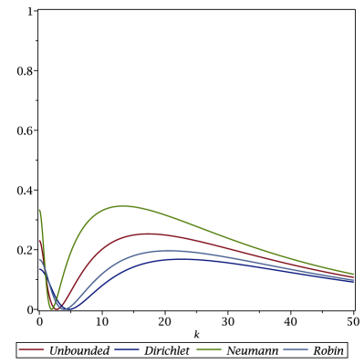
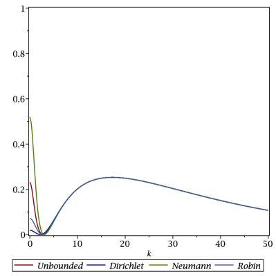
Figure 2.2: Left: optimized Schwarz convergence factor for $\eta-\Delta$ and different outer boundary conditions. Right: corresponding convergence factors when using the optimized parameter from the simpler unbounded domain analysis.

We see that the contraction factor equioscillates using the asymptotic formulas already for an overlap $L=0.02$, so the formulas are very useful in practice. We see also that the unbounded domain analysis which does not take into account the geometry leads to an optimized convergence factor in between the other ones. In practice one can also use the corresponding simpler formula from ?, namely

$$p^{*}=\frac{1}{2}(4(k_{\min}^{2}+\eta))^{1/3}L^{-1/3}$$ (29)

in the case of the screened Laplace equation, which only deteriorates the performance a little, see Figure 2.2 on the right.

Another, easy to use choice is to use a low frequency Taylor expansion about $k=0$ of the optimal symbol of the DtN operator DtNbdd, since the classical Schwarz method is not working well for low frequencies, as we have seen in Figure 2.1 on the left. Expanding the optimal DtN symbols in DtNbdd, we obtain

$$\begin{array}[]{rcl}p_{1}^{r}&=&\frac{\sqrt{\eta}\left(\tanh(\sqrt{\eta}(X_{1}^{r}-1))\sqrt{\eta}-p^{r}\right)}{\tanh(\sqrt{\eta}(X_{1}^{r}-1))p^{r}-\sqrt{\eta}}+O(k^{2}),\\ p_{2}^{l}&=&\frac{\sqrt{\eta}\left(\tanh(\sqrt{\eta}X_{2}^{l})\sqrt{\eta}+p^{l}\right)}{\tanh(\sqrt{\eta}X_{2}^{l})p^{l}+\sqrt{\eta}}+O(k^{2}).\end{array}$$ (30)

We see that the Taylor parameters also take into account the geometry. Using just the zeroth order term leads to the Taylor convergence factors shown in Figure 2.3 on the left.

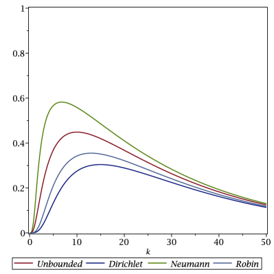
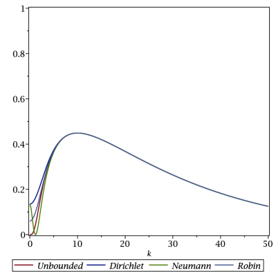
Figure 2.3: Left: convergence factor for Schwarz with Taylor based Robin transmission conditions for $\eta-\Delta$ and different outer boundary conditions on the left Right: corresponding Taylor Schwarz convergence factor using the zeroth order Taylor transmission conditions from the unbounded domain analysis, $p_{1}^{r}=p_{2}^{l}=\sqrt{\eta}$.

Their maximum $\bar{k}$ is affected by the outer boundary conditions, and can be explicitly computed when the overlap $L:=X_{2}^{l}-X_{1}^{r}$ becomes small,

$$\bar{k}\sim\frac{\sqrt{p_{1}^{r}+p_{2}^{l}}}{\sqrt{L}},\quad\rho\sim 1-4\sqrt{p_{1}^{r}+p_{2}^{l}}\sqrt{L},$$ (31)

where $p_{1}^{r}$ and $p_{2}^{l}$ are from (30) without the order term, and setting $X_{1}^{r}:=X_{2}^{l}$ in $p_{1}^{r}$ due to the expansion for $L$ small.

On the right, we show the results when using the first term in the Robin transmission conditions from the Taylor expansion of the optimal symbols from the unbounded domain analysis, $\sqrt{k^{2}+\eta}=\sqrt{\eta}+\frac{1}{2\sqrt{\eta}}k^{2}+O(k^{4})$, i.e. $p_{1}^{r}=p_{2}^{l}=\sqrt{\eta}$. We see that this choice works even better compared to the precise Taylor coefficients adapted to the outer boundary conditions in the Neumann case, but slightly worse for the Dirichlet and Robin case. Nevertheless, convergence with the simple Taylor conditions is not as good as with the optimized ones in Figure 2.2, and this becomes more pronounced when the overlap $L$ becomes small as shown in (31) compared to (28). Higher order transmission conditions can also be used and analyzed, see ?, and give even better performance with weaker asymptotic dependence on the overlap.

2.2 Helmholtz problems

We now investigate what changes if the equation is the Helmholtz equation,

$$(\Delta+\omega^{2})u=f\quad\mbox{in $\Omega:=(0,1)\times(0,Y)$},$$ (32)

with $\omega\in\mathbb{R}$. As boundary conditions, we impose on the left and right again the Robin boundary condition bclr, and on top and bottom first a Dirichlet or a Neumann condition as in bctb. The alternating Schwarz method remains as in SMDT, but with the differential operator $(\eta-\Delta)$ replaced by the Helmholtz operator $(\Delta+\omega^{2})$. The corresponding error equations for the Fourier coefficients are

$$(\partial_{xx}+\omega^{2}-k^{2})\hat{e}_{1}^{n} =0 \mbox{in $(0,X_{1}^{r})$}, (\partial_{xx}+\omega^{2}-k^{2})\hat{e}_{2}^{n} =0 \mbox{in $(X_{2}^{l},1)$},$$ (33)

$$\beta_{1}^{r}(\hat{e}_{1}^{n}) =\beta_{1}^{r}(\hat{e}_{2}^{n-1}) \mbox{at $x=X_{1}^{r}$}, \beta_{2}^{l}(\hat{e}_{2}^{n}) =\beta_{2}^{l}(\hat{e}_{1}^{n}) \mbox{at $x=X_{2}^{l}$},$$

$$\beta^{l}(\hat{e}_{1}^{n}) =0 \mbox{at $x=0$}, \beta^{r}(\hat{e}_{2}^{n}) =0 \mbox{at $x=1$}.$$

Solving the ordinary differntial equations, we obtain using the outer Robin boundary conditions for each Fourier mode $k\neq\pm\omega$ the solutions ($\underline{x}:=1-x$)

$$\hat{e}_{1}^{n}(x,k) =A_{1}^{n}(k)\left({\sqrt{\omega^{2}-k^{2}}\cos(\sqrt{\omega^{2}-k^{2}}x)+p^{l}\sin(\sqrt{\omega^{2}-k^{2}}x)}\right),$$ (34)

$$\hat{e}_{2}^{n}(x,k) =A_{2}^{n}(k)\left({\sqrt{\omega^{2}-k^{2}}\cos(\sqrt{\omega^{2}-k^{2}}\underline{x})+p^{r}\sin(\sqrt{\omega^{2}-k^{2}}\underline{x})}\right).$$

Comparing with the solutions for the screened Laplace equation in ScreenedLaplaceSols, we see that the hyperbolic sines and cosines are simply replaced by the normal sines and cosines, which shows that the solutions are oscillatory, instead of decaying. Note however that the arguments of the sines and cosines are only real if $k^{2}<\omega^{2}$, i.e. for Fourier modes below the frequency parameter $\omega$. For larger Fourier frequencies, the argument becomes imaginary, and the sines and cosines need to be replaced by their hyperbolic variants and we obtain that solutions behave like for the screened Laplace problem in ScreenedLaplaceSols.

The two remaining constants $A_{1}^{n}(k)$ and $A_{2}^{n}(k)$ are determined again using the transmission conditions, and we obtain after a short calculation again the convergence factor of the form RhoOSM, with

$$\begin{array}[]{rcl}\rho_{1}&=&\frac{(k^{2}-\sigma_{1}^{r}p^{r}-\omega^{2})\sin(\sqrt{\omega^{2}-k^{2}}(X_{1}^{r}-1))-\cos(\sqrt{\omega^{2}-k^{2}}(X_{1}^{r}-1))\sqrt{\omega^{2}-k^{2}}(p^{r}-\sigma_{1}^{r})}{(k^{2}+\sigma_{1}^{r}p^{l}-\omega^{2})\sin(\sqrt{\omega^{2}-k^{2}}X_{1}^{r})+\cos(\sqrt{\omega^{2}-k^{2}}X_{1}^{r})\sqrt{\omega^{2}-k^{2}}(p^{l}+\sigma_{1}^{r})},\\ \rho_{2}&=&\frac{(k^{2}-\sigma_{2}^{l}p^{l}-\omega^{2})\sin(\sqrt{\omega^{2}-k^{2}}X_{2}^{l})+\cos(\sqrt{\omega^{2}-k^{2}}X_{2}^{l})\sqrt{\omega^{2}-k^{2}}(p^{l}-\sigma_{2}^{l})}{(k^{2}+\sigma_{2}^{l}p^{r}-\omega^{2})\sin(\sqrt{\omega^{2}-k^{2}}(X_{2}^{l}-1))-\cos(\sqrt{\omega^{2}-k^{2}}(X_{2}^{l}-1))\sqrt{\omega^{2}-k^{2}}(p^{r}+\sigma_{2}^{l})}.\end{array}$$ (35)

It is again instructive to look at the special case first where the domain, and thus the subdomains, are unbounded on the left and right, which can be obtained from the result above by introducing for the outer Robin parameters the symbol of the DtN operator, i.e. $p^{r}:=\vartheta\I\sqrt{\omega^{2}-k^{2}}$, $p^{l}:=\vartheta\I\sqrt{\omega^{2}-k^{2}}$, where $\vartheta=\mathrm{sign}(\omega^{2}-k^{2})$ if $\sqrt{z}$ for $z\in\mathbb{C}$ uses the branch cut $(-\infty,0)$. These symbols can be obtained as shown in footnote 8 for the screened Laplace problem, and leads after simplification to the convergence factor

$$\rho(k,\omega,\sigma_{1}^{r},\sigma_{2}^{l})=\frac{\vartheta\I\sqrt{\omega^{2}-k^{2}}-\sigma_{2}^{l}}{\vartheta\I\sqrt{\omega^{2}-k^{2}}+\sigma_{2}^{l}}\,\frac{\vartheta\I\sqrt{\omega^{2}-k^{2}}-\sigma_{1}^{r}}{\vartheta\I\sqrt{\omega^{2}-k^{2}}+\sigma_{1}^{r}}e^{-2(X_{1}^{r}-X_{2}^{l})\sqrt{k^{2}-\omega^{2}}}.$$ (36)

As in the case of the screened Laplace equation, we see again that if we choose in the transmission conditions the symbol of the DtN operators, $\sigma_{1}^{r}=\sigma_{2}^{l}=\vartheta\I\sqrt{\omega^{2}-k^{2}}$, the convergence factor vanishes identically for all Fourier frequencies $k$, and we get an optimal Schwarz method, see footnote 5, as for the screened Laplace problem.

In the bounded domain case, we can still obtain an optimal Schwarz method choosing in the transmission conditions the tangential symbols of the transparent boundary conditions for the bounded subdomains, which is equivalent to choosing $\sigma_{1}^{r}$ and $\sigma_{2}^{l}$ such that $\rho_{1}$ and $\rho_{2}$ in rho12H vanish, and leads to

$$\begin{array}[]{rcl}\sigma_{1}^{r}&=&\frac{\sqrt{\omega^{2}-k^{2}}\left(-\tan(\sqrt{\omega^{2}-k^{2}}(X_{1}^{r}-1))\sqrt{\omega^{2}-k^{2}}-p^{r}\right)}{\tan(\sqrt{\omega^{2}-k^{2}}(X_{1}^{r}-1))p^{r}-\sqrt{\omega^{2}-k^{2}}},\\ \sigma_{2}^{l}&=&\frac{\sqrt{\omega^{2}-k^{2}}\left(-\tan(\sqrt{\omega^{2}-k^{2}}X_{2}^{l})\sqrt{\omega^{2}-k^{2}}+p^{l}\right)}{\tan(\sqrt{\omega^{2}-k^{2}}X_{2}^{l})p^{l}+\sqrt{\omega^{2}-k^{2}}}.\end{array}$$ (37)

As in the unbounded domain case, these values correspond to the symbols of the associated DtN operators, as one can verify by a direct computation using the solutions HelmholtzSols on their respective domains, as done for the unbounded domain case of the screened Laplace problem in footnote 8. We see that in the bounded domain case, the symbols of the DtN maps in DtNbddH, and hence the DtN maps also, depend on the outer boundary conditions, since again both the domain parameters ($X_{1}^{r}$ and $X_{2}^{l}$) and the Robin parameters in the outer boundary conditions ($p^{l}$ and $p^{r}$) appear in them. For large frequencies $k$, we still have

$$\sigma_{1}^{r}\sim\sqrt{k^{2}-\omega^{2}},\quad\sigma_{2}^{l}\sim\sqrt{k^{2}-\omega^{2}},$$

since the tangent function for imaginary argument $\I z$ becomes $\I\tanh z\to\pm\I$ as $z\to\pm\infty$, and thus high frequencies, also called evanescent modes in the Helmholtz solution, still do not see the difference from the bounded to the unbounded case, as in the screened Laplace problem.

Choosing Robin transmission conditions, ${\cal S}_{1}^{r}:=p_{1}^{r}=\sigma_{1}^{r}$ and ${\cal S}_{2}^{l}:=p_{2}^{l}=\sigma_{2}^{l}$ with $p_{1}^{r},p_{2}^{l}\in\mathbb{R}$ in TC, and taking the limit in the convergence factor RhoOSMUnbounded as the Robin parameters $p_{1}^{r}$ and $p_{2}^{l}$ go to infinity, we find

$$\rho(k,\eta,)=e^{-2(X_{1}^{r}-X_{2}^{l})\sqrt{k^{2}-\omega^{2}}},$$ (38)

which is the convergence factor of the classical alternating Schwarz method for the Helmholtz equation on the unbounded domain, and we see again the overlap $L:=X_{1}^{r}-X_{2}^{l}$ appearing in the exponential function. The classical Schwarz method therefore converges for all Fourier modes $k^{2}>\omega^{2}$, provided there is overlap. However for smaller Fourier frequencies, the method does not contract on the unbounded domain.

To see how the Schwarz method contracts on a bounded domain, we show in Figure 2.4 (left) the different cases for the outer boundary conditions ($p^{l}=p^{r}=\I\,\omega$ in the Robin case), by plotting RhoOSM for when the parameters in the Robin transmission conditions goes to infinity, and the Helmholtz frequency parameter $\omega=10$, again with overlap $L=0.02$.

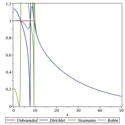
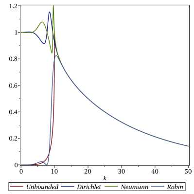
Figure 2.4: Left: classical Schwarz convergence factor for Helmholtz and different outer boundary conditions on the left and right. Right: corresponding optimized Schwarz convergence factor with Taylor transmission conditions from the unbounded domain analysis.

This shows that the different outer boundary conditions greatly influence the convergence for Fourier modes $k^{2}<\omega^{2}$, the Schwarz method violently diverges for these modes, except for the unbounded case where we obtain stagnation, but still no convergence. For larger frequencies $k^{2}>\omega^{2}$, there is no influence of the outer boundary conditions on the convergence. On the right in Figure 2.4 we show the corresponding convergence factors with Robin transmission conditions, chosen as $p_{1}^{r}=p_{2}^{l}=\I\,\omega$, which correspond to Taylor transmission conditions of order zero from the unbounded domain anaylsis, by expansion of the corresponding optimal symbol around $k=0$, $\I\sqrt{\omega^{2}-k^{2}}=\I\,\omega+O(k^{2})$. Here we see that again the different outer boundary conditions greatly influence the convergence for Fourier modes $k^{2}<\omega^{2}$: for unbounded subdomains, and also subdomains with Robin radiation conditions at the ends, the Schwarz method converges well for small Fourier frequencies. With Dirichlet and Neumann outer boundary conditions however, we obtain again divergence, although a bit less violent than in the classical Schwarz method. For larger frequencies $k^{2}>\omega^{2}$, there is again very little influence of the outer boundary conditions on the convergence. We also observe an interesting phenomenon around $k^{2}=\omega^{2}$ the so called resonnance frequency: with Robin radiation conditions, the Schwarz method also converges in this case, while for unbounded subdomains we obtain a convergence factor with modulus one there.

It does not help to use the corresponding Taylor transmission conditions of order zero adapted to each outer boundary conditions, as we show in Figure 2.5 on the left.

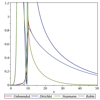
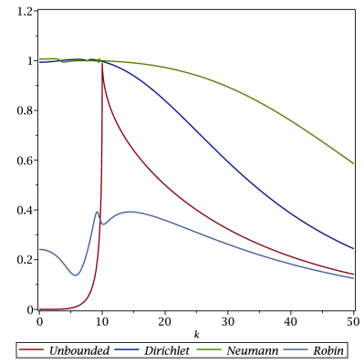
Figure 2.5: Left: optimized Schwarz convergence factor for Helmholtz and different outer boundary conditions on the left and right, using the correspondingly adapted Taylor transmission conditions. Right: corresponding optimized Schwarz convergence factor minimizing the maximum of the convergence factor numerically with complex Robin transmission conditions.

Now the low frequencies converge well in all cases, but divergence is even more violent for other frequencies with Dirichlet and Neumann outer boundary conditions. We finally show the results of numerically optimized Robin transmission conditions with $p_{1}^{r},p_{2}^{l}\in\mathbb{C}$ on the right in Figure 2.5, minimizing the convergence factor in modulus. We see that there do not exist complex Robin parameters that can make the optimized Schwarz method work well for Dirichlet and Neumann outer boundary conditions on the left and right, low frequencies simply converge badly or not at all. However with Robin outer boundary conditions on the left and right, the optimization leads to a quite fast method now, with a convergence factor bounded by $0.4$, compared to the Taylor transmission conditions where the convergence factor was bounded by about $0.8$. This shows that for Helmholtz problems absorbing boundary conditions on the original problem are very important for Schwarz methods to converge, and we thus focus on this case in what follows, i.e. $p^{l}=p^{r}=\I\omega$.

We start by studying the performance with Taylor transmission conditions, $p_{1}^{r}=p_{2}^{l}=\I\omega$, when the overlap is varying, and the Helmholtz frequency $\omega$ is increasing. We show in Figure 2.6

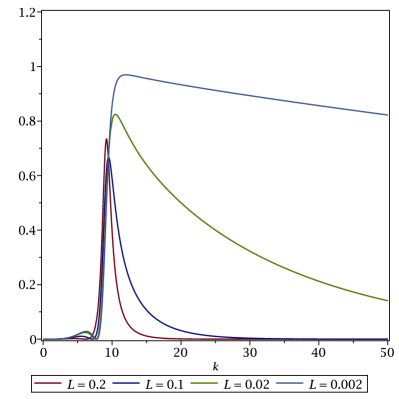
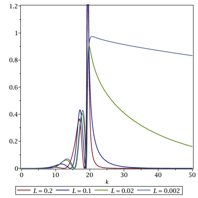
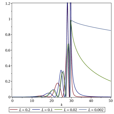
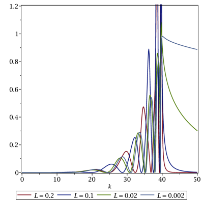
Figure 2.6: Optimized Schwarz convergence factor for Helmholtz with Robin outer boundary conditions and Taylor transmission conditions for different overlap sizes: from top left to bottom right $\omega=10,20,30,40$.

the convergence factors for four different overlap sizes $L=0.2,0.1,0.02,0.002$ and Helmholtz frequencies $\omega=10,20,30,40$. We see that convergence difficulties increase dramatically with increasing $\omega$: while for $\omega=10$, the convergence factor is smaller than one for all overlap sizes $L$, we see already that the largest overlap $L=0.2$ is not leading to better convergence than the next smaller one, $L=0.1$. For $\omega=20$ now the two larger overlaps $L=0.2$ and $L=0.1$ lead to divergence. For $\omega=30$ the best performance is obtained for the smallest overlap $L=0.002$, and for $\omega=40$ the smallest overlap is the only overlap for which the method still contracts. We thus need small overlap in this waveguide type setting with Dirichlet or Neumann conditions on top and bottom for the method to work with Taylor transmission conditions.

Let us investigate this analytically when the overlap $L$ goes to zero. Computing the location of the maximum at $\bar{k}>\omega$ visible in Figure 2.6 and then evaluating the value of the convergence factor in modulus at this frequency $\bar{k}$, we obtain for the convergence factor for small overlap $L$ after a long and technical computation

$$\max_{k}|\rho(k,\omega,L)|=1-(8-4\ln 2-4\ln L)L+O(L^{2}).$$ (39)

The method therefore converges for small enough overlap also when $\omega$ becomes large for this two subdomain decomposition and outer Robin conditions on the left and right, $p^{l}=p^{r}=\I\omega$ with Taylor transmission conditions $p_{1}^{r}=p_{2}^{l}=\I\omega$. However convergence is rather slow, compared to the case of the screened Laplace equation with convergence factor $1-O(\sqrt{L})$ as shown in (31), even though there is absorption for Helmholtz on the left and right. We show in Table 1

$L$	$\max_{k}|\rho|$	$1-\max_{k}|\rho|$
0.1000000000	22.7898956625	-21.7898956625
0.0100000000	1.2309097387	-0.2309097387
0.0010000000	0.9962177046	0.0037822954
0.0001000000	0.9987180209	0.0012819791
0.0000100000	0.9998069224	0.0001930776
0.0000010000	0.9999749357	0.0000250643
0.0000001000	0.9999969499	0.0000030501
0.0000000100	0.9999996424	0.0000003576
0.0000000010	0.9999999591	0.0000000409
0.0000000001	0.9999999954	0.0000000046

Table 1: Maximum of the convergence factor for Taylor transmission conditions with the same outer boundary conditions on the left and right and $\omega=100$, for decreasing overlap size $L$.

the convergence factor for $\omega=100$ when $L$ goes to zero for a symmetric subdomain decomposition, $X_{2}^{l}=\frac{1}{2}-L/2$, $X_{1}^{r}=\frac{1}{2}+L/2$, and one can clearly see the logarithmic term $\ln L$ in the last column which displays $1-\max_{k}|\rho|$, from the slow increase in the first non-zero digit. One can also see from Table 1 that for a given Helmholtz frequency $\omega$, there is an optimal choice for the overlap, here around $L=0.001$ for best performance.

We next investigate if an optimized choice of the complex transmission parameters $p_{1}^{r},p_{2}^{l}\in\mathbb{C}$ can further improve the convergence behavior with Robin conditions with $p^{r}=p^{l}=\I\omega$ on the left and right outer boundaries. A numerical optimization minimizing the maximum of the convergence factor gives the results shown in Figure 2.7.

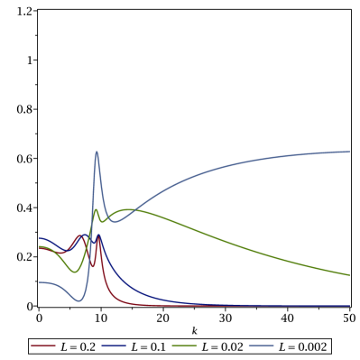
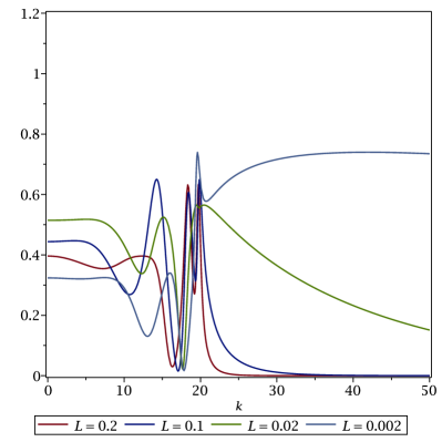
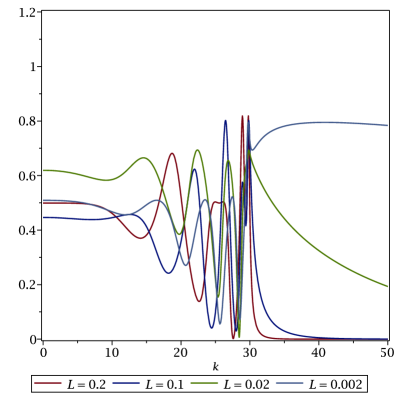
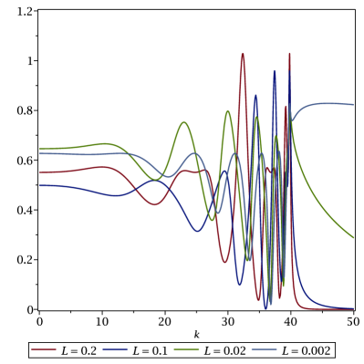
Figure 2.7: Optimized Schwarz convergence factor for Helmholtz with Robin outer boundary conditions and optimized complex Robin transmission conditions for different overlap sizes: from top left to bottom right $\omega=10,20,30,40$.

Comparing with the corresponding Figure 2.6 for the Taylor transmission conditions, we see that much better contraction factors can be obtained using the optimized transmission conditions, and also that the method is convergent for all overlaps for $\omega=10,20,30$. However, for $\omega=40$, we see again that for the largest overlap, the optimized contraction factor is above $1$, and thus as in the Taylor transmission conditions, for large Helmholtz frequency $\omega$, the overlap will need to be small enough for the optimized method to converge, and there will be a best choice for the overlap.

To investigate this further, we show in Table 2 the best contraction factor that can be obtained for $\omega=100$, as we did in Table 1 for the Taylor transmission conditions, and we also show the value of the optimized complex transmission condition parameter.

$L$	$p_{1}^{r}=p_{2}^{l}$	$\max_{k}|\rho|$	$1-\max_{k}|\rho|$
0.1000000000	-13.7512+17.6068	1.366317	-0.366317
0.0100000000	-0.7183+26.7434	0.963833	0.036166
0.0010000000	0.7700+7.8147	0.882396	0.117603
0.0001000000	1.6590+11.5704	0.929865	0.070134
0.0000100000	3.6059+24.6349	0.966615	0.033384
0.0000010000	7.7838+52.9876	0.984342	0.015657
0.0000001000	16.7767+114.0584	0.992699	0.007300
0.0000000100	36.1477+245.6848	0.996604	0.003395
0.0000000010	77.8794+529.2904	0.998422	0.001577
0.0000000001	167.7869+1140.3116	0.999267	0.000732

Table 2: Best complex parameter choice and maximum of the convergence factor for optimized complex Robin transmission conditions with outer Robin boundary conditions $p^{l}=p^{r}=\I\omega$ on the left and right and $\omega=100$, for decreasing overlap size $L$.

We see that the optimization leads to a method which degrades much less, compared to the Taylor transmission conditions, and there is still a best choice for the overlap that leads to the most advantageous contraction, around overlap $L=0.001$ as in the Taylor case. But using the optimized parameters the method will converge approximately $100$ times faster, since $0.9987180208^{100}=0.879607\approx 0.882396$. There are however so far no analytical asymptotic formulas for this optimized choice available. Nevertheless, plotting the results from Table 2 in Figure 2.8

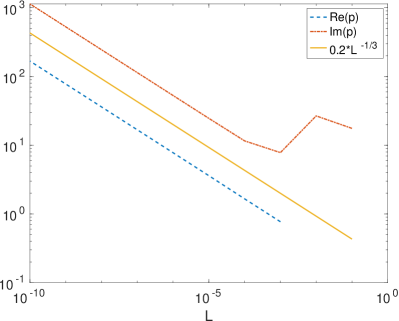
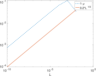
Figure 2.8: Asymptotic behavior of the optimized complex Robin parameter and associated convergence factor distance from $1$.

cleary shows that the optimized choice behaves asymptotically for small overlap $L$ as

$$p_{1}^{r}\sim(C_{1}^{r}+\I\tilde{C}_{1}^{r})L^{-1/3},\quad p_{2}^{l}\sim(C_{2}^{l}+\I\tilde{C}_{2}^{l})L^{-1/3},\quad\max_{k}|\rho|=1-O(L^{1/3}),$$ (40)

which is a much better result than for the Taylor transmission conditions that gave $\max_{k}|\rho|=1-O(L)$ up to the logarithmic term.

Since we have seen how important absorption is for the Helmholtz problem, in contrast to the screened Laplace problem, we now study the Helmholtz problem also with Robin conditions all around, also on top and bottom. This needs the solution of the corresponding Sturm-Liuville problem (details can be found in Section 3). We start again by studying the performance with Taylor transmission conditions, $p_{1}^{r}=p_{2}^{l}=\I\omega$, when the overlap is varying, and the Helmholtz frequency $\omega$ is increasing. We show in Figure 2.9

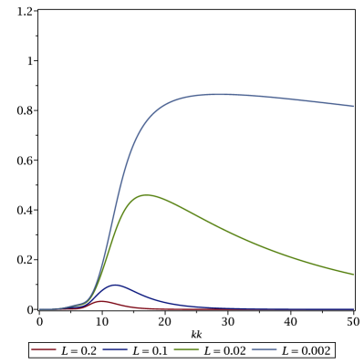
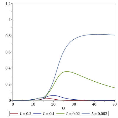
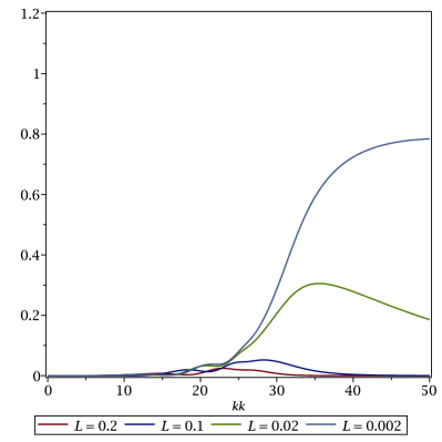
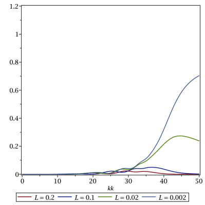
Figure 2.9: Optimized Schwarz convergence factor for Helmholtz with Robin outer boundary conditions all around and Taylor transmission conditions for different overlap sizes: from top left to bottom right $\omega=10,20,30,40$.

the convergence factors for four different overlap sizes $L=0.2,0.1,0.02,0.002$ and Helmholtz frequencies $\omega=10,20,30,40$. We see immediately the tremendous improvement by having now also Robin conditions on the top and bottom in the Helmholtz equation: the Schwarz method converges for all overlap sizes $L$, even if the Helmholtz frequency is increaseing, there is no requirement any more for the overlap $L$ to be small. We do currently not yet have an analysis of this behavior, but we show in Table 3

$L$	$\max_{k}|\rho|$	$1-\max_{k}|\rho|$
0.1000000000	0.0471851340	0.9528148659
0.0100000000	0.3360508362	0.6639491637
0.0010000000	0.7854583112	0.2145416887
0.0001000000	0.9537799195	0.0462200804
0.0000100000	0.9913446318	0.0086553681
0.0000010000	0.9984392375	0.0015607624
0.0000001000	0.9997213603	0.0002786396
0.0000000100	0.9999503928	0.0000496071
0.0000000010	0.9999911753	0.0000088246
0.0000000001	0.9999984305	0.0000015694

Table 3: Maximum of the convergence factor for Taylor transmission conditions with the same Robin outer boundary conditions all around and $\omega=100$, for decreasing overlap size $L$.

the convergence factor for $\omega=100$ when $L$ goes to zero for a symmetric subdomain decomposition, $X_{2}^{l}=\frac{1}{2}-L/2$, $X_{1}^{r}=\frac{1}{2}+L/2$, and one can clearly see the much better asymptotic performance due to the Robin boundary conditions on top and bottom, compared to the waveguide case shown in Table 1. We can also numerically observe the dependence of the convergence factor in this case to be

$$\max_{k}|\rho(k,\omega,L)|=1-O(L^{3/4})$$ (41)

as we show in Figure 2.10

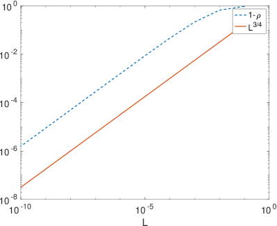
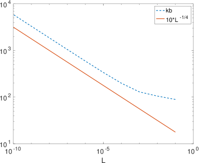
Figure 2.10: Asymptotic behavior of the convergence factor with Robin conditions all around (left) and of the maximum location $\bar{k}$ (right).

on the left. On the right, we show how the maximum location $\bar{k}=O(L^{-1/4})$ is increasing now.

We next show that an optimized choice of the complex transmission parameters $p_{1}^{r},p_{2}^{l}\in\mathbb{C}$ can still further improve the convergence behavior with Robin conditions all around the global domain. A numerical optimization minimizing the maximum of the convergence factor gives the results shown in Figure 2.11.

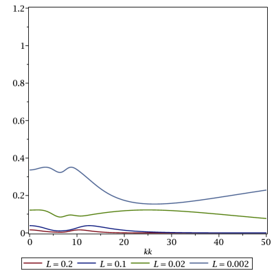
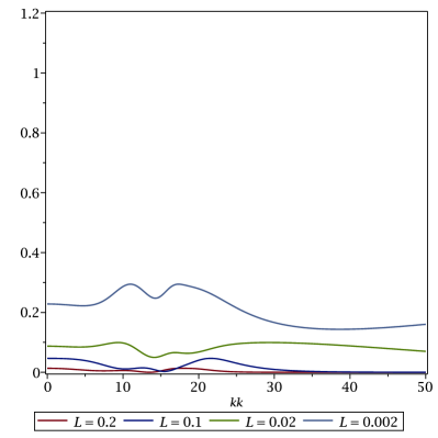
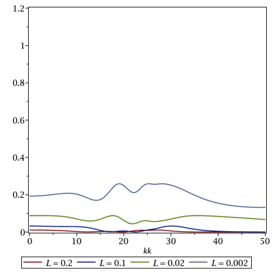
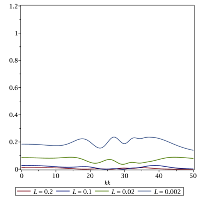
Figure 2.11: Optimized Schwarz convergence factor for Helmholtz with Robin outer boundary conditions all around and optimized complex Robin transmission conditions for different overlap sizes: from top left to bottom right $\omega=10,20,30,40$.

Comparing with the corresponding Figure 2.9 for the Taylor transmission conditions, we see that again much better contraction factors can be obtained using the optimized transmission conditions. To investigate this further, we show in Table 4 the best contraction factor that can be obtained for $\omega=100$, as we did in Table 3 for the Taylor transmission conditions, and we also show the value of the optimized complex transmission condition parameter.

$L$	$p_{1}^{r}=p_{2}^{l}$	$\max_{k}|\rho|$	$1-\max_{k}|\rho|$
0.1000000000	0.0002+82.4166	0.057800	0.942200
0.0100000000	0.0003+50.8853	0.292866	0.707134
0.0010000000	47.7606+79.4621	0.301674	0.698326
0.0001000000	120.2543+142.8230	0.538849	0.461151
0.0000100000	266.8504+287.5608	0.746725	0.253275
0.0000010000	578.4744+609.4633	0.872807	0.127193
0.0000001000	1247.9382+1308.2677	0.938763	0.061237
0.0000000100	2689.3694+2816.3510	0.971090	0.028910
0.0000000010	5794.4274+6066.6093	0.986475	0.013525
0.0000000001	12483.8801+13069.6327	0.993699	0.006301

Table 4: Best complex parameter choice and maximum of the convergence factor for optimized complex Robin transmission conditions with outer Robin boundary conditions all around and $\omega=100$, for decreasing overlap size $L$.

We see that the optimization leads to a method which again degrades much less, compared to the Taylor transmission conditions, and the best choice is the largest overlap when there are Robin conditions all around the domain. There are currently no analytical asymptotic formulas for this optimized choice either, but plotting the results from Table 4 in Figure 2.12

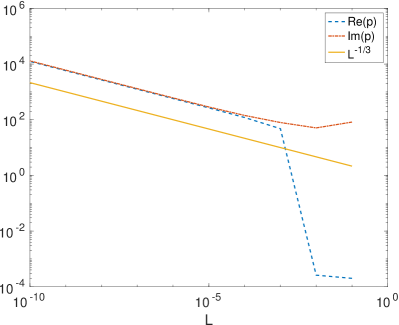
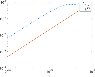
Figure 2.12: Asymptotic behavior of the optimized complex Robin parameter and associated convergence factor distance from $1$ when there are Robin conditions all around the domain.

cleary shows that the optimized choice behaves asymptotically for small overlap $L$ again as

$$p_{1}^{r}\sim(C_{1}^{r}+\I\tilde{C}_{1}^{r})L^{-1/3},\quad p_{2}^{l}\sim(C_{2}^{l}+\I\tilde{C}_{2}^{l})L^{-1/3},\quad\max_{k}|\rho|=1-O(L^{1/3}),$$ (42)

like in the waveguide case with Dirichlet or Neumann conditions on top and bottom. This is still much better than for the Taylor transmission conditions that gave $\max_{k}|\rho|=1-O(L^{3/4})$.

From the two subdomain analysis in this section, we have already learned many things for Schwarz methods by domain truncation, or optimized Schwarz methods: for the screened Laplace problem, outer boundary conditions are not influencing convergence very much, and complete analysis is available for the convergence of these methods, also with optimized formulas for Robin transmission conditions. Compared to classical Schwarz methods with contraction factors $1-O(L)$ when the overlap $L$ becomes small, Taylor transmission conditions give a contraction factor $1-O(\sqrt{L})$, and optimized Robin transmission conditions give $1-O(L^{1/3})$. This is very different for the Helmholtz case, where the performance of Schwarz methods is very much dependent on the outer boundary conditions imposed on the domain on which the problem is considered. Radiation boundary conditions are very important for Schwarz methods to function here: in a waveguide setting with Robin conditions on the left and right, classical Schwarz methods still do not work, but Taylor transmission conditions of Robin type, the simplest absorbing boundary conditions, can then lead to convergent Schwarz methods, provided the overlap is small enough, with convergence factor $1-O(L)$ up to a logarithmic term. Optimized Robin transmission conditions lead again to $1-O(L^{1/3})$, as in the screened Laplace case. If there are radiation conditions of Robin type all around, using these same conditions also as transmission conditions leads to contraction factors of the form $1-O(L^{3/4})$, but now the methods also work with larger overlap, and optimized Robin conditions give $1-O(L^{1/3})$ with numerically observed much better constants, asymptotically comparable to the screened Laplace case!

3 Many subdomain analysis

We now investigate the performance of optimized Schwarz methods, or equivalently Schwarz methods by domain truncation, when more than two subdomains are used. Since we have seen in Section 2 that absorbing boundary conditions (ABCs) play an important role for the Helmholtz case, and perfectly matched layers (PMLs) are another technique to truncate domains, we now study the convergence of Schwarz methods for a sligthly more general problem where the operators in the $x$ and $y$ direction are written separately, so that PML modifications can be introduced, namely

$$(\mathcal{L}_{x}+\mathcal{L}_{y})u+\eta u =f \text{ on }\Omega=[0,X]\times[0,Y],$$ (43)

$$\mathcal{B}^{l}u =0 \text{ on }\{0\}\times[0,Y],$$

$$\mathcal{B}^{r}u =0 \text{ on }\{X\}\times[0,Y],$$

$$\mathcal{B}^{b}u =0 \text{ on }[0,X]\times\{0\},$$

$$\mathcal{B}^{t}u =0 \text{ on }[0,X]\times\{Y\},$$

where $\mathcal{L}_{*}$ is a linear partial differential operator about $*$, $\eta$ is a constant which we will choose to handle both the screened Laplace and the Helmholtz case, the unknown $u$ and the data $f$ are functions on $\Omega$, and $\mathcal{B}^{*}$’s are linear trace operators. For Schwarz methods, the domain is decomposed first into $N$ subdomains $[X_{j}^{l},X_{j}^{r}]\times[0,Y]$ with $X_{j}^{l}=(j-1)H$, $X_{j}^{r}=jH+2L$ and $H=(X-2L)/N$, as shown for an example in Figure 1.2 on the right. The restriction of eqprb onto the subdomains $\Omega_{j}$ are solved with the solutions $u_{j}$ to satisfy the transmission conditions

$$\mathcal{B}_{j}^{l,r}u_{j}=\mathcal{B}_{j}^{l,r}u_{j\mp 1}\text{ on }\{X_{j}^{l,r}\}\times[0,Y],$$ (44)

except on the original boundary $\{0,X\}\times[0,Y]$.

Remark 3.1

We note that if $u_{j}$ satisfies the restriction of eqprb onto $\Omega_{j}$, by linearity of eqprb, the partial differential equation for the error $u-u_{j}$ on $\Omega_{j}$ is homogeneous (with $f=0$) and invariant under the transformation $(x,y,\eta)\mapsto(\frac{x}{Y},\frac{y}{Y},Y^{2}\eta)$. We further assume that the boundary and transmission conditions have the same invariance. Then, we can let $Y=1$ without loss of generality for the convergence analysis.

The generalised Fourier frequencies $\pm\xi$ correspond to the square-roots of the Sturm-Liouville eigenvalues $\xi^{2}$,

$$\mathcal{L}_{y}\phi =\xi^{2}\phi \text{ on }[0,Y],$$ (45)

$$\mathcal{B}^{b}\phi =0 \text{ at }\{0\},$$

$$\mathcal{B}^{t}\phi =0 \text{ at }\{Y\}.$$

We assume that the eigenfunctions $\{\phi(y,\xi_{n})\}$, $\xi\in\{\xi_{0},\xi_{1},\xi_{2},\ldots\}\subset\mathbb{C}$ allow the solution of eqprb to be represented as $\sum_{n=0}^{\infty}u(x,\xi_{n})\phi(y,\xi_{n})$, with $u(x,\xi)$ satisfying the problem

$$\mathcal{L}_{x}u+(\xi^{2}+\eta)u =f\quad \mbox{on }[0,X],$$ (46)

$$\mathcal{B}^{l}u =0\quad \mbox{at }x=0,$$

$$\mathcal{B}^{r}u =0\quad \mbox{at }x=X.$$

Let $g_{j}^{l}:=\mathcal{B}_{j}^{l}u_{j}$ at $x=X_{j}^{l}$ and $g_{j}^{r}:=\mathcal{B}_{j}^{r}u_{j}$ at $x=X_{j}^{r}$. To rewrite eqtc in terms of the interface data $g_{2}^{l},\ldots,g_{N}^{l},g_{1}^{r},\ldots,g_{N-1}^{r}$, i.e. in substructured form, we define the interface-to-interface operators (see also Figure 3.1)

$$a_{j}: \left(\ell_{j}\mbox{\ at }x=X_{j}^{l}\right)\rightarrow\left(\mathcal{B}_{j+1}^{l}v_{j}\mbox{\ at }x=X_{j+1}^{l}\right)\ \mbox{with $v_{j}$ solving}$$

$$\mathcal{L}_{x}v_{j}+(\xi^{2}+\eta)v_{j}=0\text{ in $(X_{j}^{l},X_{j}^{r})$},\;\,\mathcal{B}_{j}^{l}v_{j}=\ell_{j}\text{ at $x=X_{j}^{l}$},\;\,\mathcal{B}_{j}^{r}v_{j}=0\text{ at $x=X_{j}^{r}$},$$

$$b_{j}: \left(\gamma_{j}\mbox{\ at }x=X_{j}^{r}\right)\rightarrow\left(\mathcal{B}_{j+1}^{l}v_{j}\mbox{\ at }x=X_{j+1}^{l}\right)\ \mbox{with $v_{j}$ solving}$$

$$\mathcal{L}_{x}v_{j}+(\xi^{2}+\eta)v_{j}=0\text{ in $(X_{j}^{l},X_{j}^{r})$},\;\,\mathcal{B}_{j}^{l}v_{j}=0\text{ at $x=X_{j}^{l}$},\;\,\mathcal{B}_{j}^{r}v_{j}=\gamma_{j}\text{ at $x=X_{j}^{r}$},$$

$$c_{j}: \left(\gamma_{j}\mbox{\ at }x=X_{j}^{r}\right)\rightarrow\left(\mathcal{B}_{j-1}^{r}v_{j}\mbox{\ at }x=X_{j-1}^{r}\right)\ \mbox{with $v_{j}$ solving}$$

$$\mathcal{L}_{x}v_{j}+(\xi^{2}+\eta)v_{j}=0\text{ in $(X_{j}^{l},X_{j}^{r})$},\;\,\mathcal{B}_{j}^{l}v_{j}=0\text{ at $x=X_{j}^{l}$},\;\,\mathcal{B}_{j}^{r}v_{j}=\gamma_{j}\text{ at $x=X_{j}^{r}$},$$

$$d_{j}: \left(\ell_{j}\mbox{\ at }x=X_{j}^{l}\right)\rightarrow\left(\mathcal{B}_{j-1}^{r}v_{j}\mbox{\ at }x=X_{j-1}^{r}\right)\ \mbox{with $v_{j}$ solving}$$

$$\mathcal{L}_{x}v_{j}+(\xi^{2}+\eta)v_{j}=0\text{ in $(X_{j}^{l},X_{j}^{r})$},\;\,\mathcal{B}_{j}^{l}v_{j}=\ell_{j}\text{ at $x=X_{j}^{l}$},\;\,\mathcal{B}_{j}^{r}v_{j}=0\text{ at $x=X_{j}^{r}$},$$

where $\mathcal{B}_{1}^{l}:=\mathcal{B}^{l}$ and $\mathcal{B}_{N}^{r}:=\mathcal{B}^{r}$. Using these operators, we can rewrite eqtc as a linear system, namely

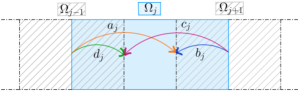
Figure 3.1: Illustration of the interface-to-interface operators.

$${\footnotesize\left[\begin{array}[]{cccc|cccc}1\vphantom{g_{1}^{l}}&&&&-b_{1}&&&\\ -a_{2}&1\vphantom{g_{2}^{l}\ddots}&&&&-b_{2}&&\\ &\ddots&\ddots\vphantom{\vdots}&&&&\ddots&\\ &&-a_{N-1}&1\vphantom{g_{N}^{l}}&&&&-b_{N-1}\\ \hline\cr-d_{2}&&&&1\vphantom{g_{2}^{r}}&-c_{2}&&\\ &-d_{3}&&&&1\vphantom{g_{3}^{r}}&\ddots&\\ &&\ddots&&&&\ddots&-c_{N-1}\vphantom{\vdots}\\ &&&-d_{N}&&&&1\vphantom{g_{N-1}^{r}}\end{array}\right]\left[\begin{array}[]{c}g_{2}^{l}\\ g_{3}^{l}\vphantom{\ddots}\\ \vdots\\ g_{N}^{l}\\ \hline\cr g_{1}^{r}\\ g_{2}^{r}\vphantom{\ddots}\\ \vdots\\ g_{N-1}^{r}\end{array}\right]=\left[\begin{array}[]{c}\tau_{2}^{l}\\ \tau_{3}^{l}\vphantom{\ddots}\\ \vdots\\ \tau_{N}^{l}\\ \hline\cr\tau_{1}^{r}\\ \tau_{2}^{r}\vphantom{\ddots}\\ \vdots\\ \tau_{N-1}^{r}\end{array}\right],}$$ (47)

which we denote by

$$\begin{bmatrix}I-A&-B\\ -D&I-C\end{bmatrix}\begin{bmatrix}g^{l}\\ g^{r}\end{bmatrix}=\begin{bmatrix}\tau^{l}\\ \tau^{r}\end{bmatrix},$$ (48)

where $\tau_{j}^{l}:=\mathcal{B}_{j}^{l}v_{j-1}$, $\tau_{j}^{r}:=\mathcal{B}_{j}^{r}v_{j+1}$ with $v_{j}$ satisfying

$$\mathcal{L}_{x}v_{j}+(\xi^{2}+\eta)v_{j} =f\quad \mbox{on }[X_{j}^{l},X_{j}^{r}],$$

$$\mathcal{B}_{j}^{l}v_{j} =0\quad \mbox{at $x=X_{j}^{l}$},$$

$$\mathcal{B}_{j}^{r}v_{j} =0\quad \mbox{at $x=X_{j}^{r}$}.$$

The double sweep Schwarz method amounts to a block Gauss-Seidel iteration for eq:bp: given an initial guess $g^{r,0}$ of $g^{r}$, we compute for iteration index $m=0,1,\ldots$

$$g^{r,m+1}:=(I-C)^{-1}\left[\tau^{r}+D(I-A)^{-1}(\tau^{l}+Bg^{r,m})\right].$$ (49)

We denote by $\epsilon^{r,m}:=g^{r}-g^{r,m}$ the error, which then by eq:gs satisfies a recurrence relation with iteration matrix $T_{\rm{DOSM}}$,

$$\epsilon^{r,m+1}=T_{\rm{DOSM}}\epsilon^{r,m}:=(I-C)^{-1}D(I-A)^{-1}B\epsilon^{r,m}.$$ (50)

The Jacobi iteration for eq:gp gives the parallel Schwarz method with the recurrence relation

$$\epsilon^{m+1}=T_{\rm{POSM}}\epsilon^{m}:=\begin{bmatrix}A&B\\ D&C\end{bmatrix}\begin{bmatrix}\epsilon^{l,m}\\ \epsilon^{r,m}\end{bmatrix}.$$ (51)

Remark 3.2

The block Jacobi iteration for eq:bp leads to the X (cross) sweeps (?, ?, ?) starting from the first and last subdomains simultaneously, namely,

$$\epsilon^{m+1}=T_{\rm{COSM}}\epsilon^{m}:=\begin{bmatrix}O&(I-A)^{-1}B\\ (I-C)^{-1}D&O\end{bmatrix}\begin{bmatrix}\epsilon^{l,m}\\ \epsilon^{r,m}\end{bmatrix}.$$ (52)

It is easy to see that $T_{\rm{COSM}}^{2}$ has the same spectra as $T_{\rm{DOSM}}$ does.

Remark 3.3

For two subdomains $N=2$, eq:gp reduces to

$$\begin{bmatrix}1&-b_{1}\\ -d_{2}&1\end{bmatrix}\begin{bmatrix}g_{2}^{l}\\ g_{1}^{r}\end{bmatrix}=\begin{bmatrix}\tau_{2}^{l}\\ \tau_{1}^{r}\end{bmatrix}.$$

Then, $T_{\rm{DOSM}}=b_{1}d_{2}$ is exactly the two-subdomain convergence factor RhoOSM. On the one hand, the influence of the outer left/right boundary conditions $\mathcal{B}^{l,r}u=0$ is totally contained in $b_{1}$ and $d_{N}$. For fast convergence, the $b_{j}$ and $d_{j}$ are the only entries that can be made arbitrarily small by approximating the transparent transmission conditions. On the other hand, the influence of $N$ is mainly through $(I-C)^{-1}$, $(I-A)^{-1}$ in eq:Tdosm or the nilpotent $A$, $C$ in eq:Tposm, not directly related to the diagonal $B$, $D$. This explains why and how the two-subdomain analysis from Section 2 is useful.

Let $s:=\sqrt{\xi^{2}+\eta}$ be the symbol of the square-root operator $\sqrt{\mathcal{L}_{y}+\eta}$ (also known as the half-plane Dirichlet-to-Neumann operator, see footnote 8). Assume the boundary operator $\mathcal{B}_{*}^{l,r}$ has the symbol $\mp q_{*}^{l,r}(\xi)\partial_{x}+p_{*}^{l,r}(\xi)$. Then, one can find the symbols of the operators $a_{j}$, $b_{j}$, $c_{j}$ and $d_{j}$ in eq:gp so that the iteration matrices $T_{\rm{POSM}}$ and $T_{\rm{DOSM}}$ become symbol matrices; see e.g. ?, ?, ?. Let

$$\mathfrak{A}=\begin{bmatrix}A&O\\ O&O\end{bmatrix},\mathfrak{B}=\begin{bmatrix}O&B\\ O&O\end{bmatrix},\mathfrak{C}=\begin{bmatrix}O&O\\ O&C\end{bmatrix},\mathfrak{D}=\begin{bmatrix}O&O\\ D&O\end{bmatrix}.$$

There exist the following results in norm.

Theorem 3.4 (?)

Let $\|\cdot\|$ be an algebra norm of matrices (so that the submultiplicative property $\|AB\|\leq\|A\|\|B\|$ holds), with $\|I\|=1$. If for some $\xi$ we have

$${\varrho}(\xi):=\|\mathfrak{B}(\xi)\|\|\mathfrak{D}(\xi)\|\left(\sum_{n=0}^{N-2}\|\mathfrak{A}(\xi)\|^{n}\right)\left(\sum_{n=0}^{N-2}\|\mathfrak{C}(\xi)\|^{n}\right)<1,$$

then the estimates

$$\|T_{\rm{POSM}}^{n}(\xi)\| \leq C_{0}(\xi)\frac{1}{1-{\varrho}(\xi)}{\varrho}(\xi)^{\left[\frac{n}{2N-2}-\frac{3}{2}\right]}, \forall n\geq 2N,$$

$$\|T_{\rm{DOSM}}^{n}(\xi)\| \leq C_{0}(\xi)(1+{\varrho}(\xi)){\varrho}(\xi)^{n-1}, \forall n\geq 2,$$

hold with $C_{0}(\xi)=\left(1+\frac{{\varrho}(\xi)}{\|\mathfrak{B}(\xi)\|}\right)\left(1+\frac{{\varrho}(\xi)}{\|\mathfrak{D}(\xi)\|}+\frac{{\varrho}(\xi)}{\|\mathfrak{B}(\xi)\|\|\mathfrak{D}(\xi)\|}\right)$.

This theorem tells us the optimized Schwarz methods converge as soon as $|b_{j}|$, $|d_{j}|$ are sufficiently small while $|a_{j}|,|c_{j}|$ remain bounded, which corresponds to having nearly transparent conditions on the left and right boundaries of each subdomain. The upper bounds suggest that a double sweep iteration $T_{\mathrm{DOSM}}$ is worth $2N-2$ parallel iterations $T_{\mathrm{POSM}}^{2N-2}$. But since we do not know how sharp the bounds are, we can still not answer precisely the scalability questions such as the scaling with $N\to\infty$. For that purpose, we opt to calculate the eigenvalues of the symbol matrices numerically. In case of $T_{\rm{DOSM}}$ with real-valued symbols, a two-sided estimate is also available (?).

Let $\rho=\rho(\xi,\eta,N,H,L,\ldots)$ be the spectral radius of the symbol iteration matrix, where the dots represent the parameters to be introduced in the transmission operator $\mathcal{B}^{l,r}_{j}$. The goal of this section is to find the asymptotic scalings of $\max_{\xi}\rho$ in terms of $\eta$, $N$, $H$, $L$, etc. One scaling is $N\to\infty$ with $\mathcal{B}^{l,r}=\mathcal{B}_{j}^{l,r}$ and $\eta$, $H$, $L$ fixed (or generally all the symbol values $a$, $b$ fixed). Another scaling is to fix $X$ and let $N\to\infty$ with $\eta$ either fixed or growing. In this scaling, $H=(X-2L)/N\to 0$ and $L=CH^{\nu}$ ($\nu\geq 1$). To distinguish the effects of $N\to\infty$ and $H\to 0$, it is useful to study a third scaling with $H\to 0$, $L=CH^{\nu}$ and all the other parameters fixed. In particular, for $N=\infty$, we can see how the subdomain size (or block size in the matrix language) influences the convergence. Also, the effect of small overlap can be revealed with $L\to 0$ and $N$, $X$ fixed.

For the parallel Schwarz iteration with $a_{j}=a$, $b_{j}=b$, $c_{j}=c$, $d_{j}=d$ independent of $j$ and $a=c$, a closed formula for $\rho_{\infty}:=\lim_{N\to\infty}\rho$ has been found rigorously (?), which we shall use later. Here, we give a formal derivation when the domain becomes $(-\infty,\infty)\times(0,Y)$ and $\Omega_{j}=(X_{j}^{l},X_{j}^{r})\times(0,Y)$ for $j=0,\pm 1,\pm 2,...$. The interface data are collected as the bi-infinite sequence $g:=(\ldots,g_{j}^{l},g_{j-1}^{r},g_{j+1}^{l},g_{j}^{r},\ldots)$ with the displayed four entries indexed by $2j-1$, $2j$, $2j+1$ and $2j+2$. We define the splitted Fourier sequences (entries displayed at the same indices as before)

$$\phi_{\mu,1} :=(\ldots,\mathrm{e}^{\mathrm{i}\mu(2j-1)},0,\mathrm{e}^{\mathrm{i}\mu(2j+1)},0,\ldots),$$

$$\phi_{\mu,2} :=(\ldots,0,\mathrm{e}^{\mathrm{i}\mu(2j)},0,\mathrm{e}^{\mathrm{i}\mu(2j+2)},\ldots),$$

with $\mu\in[-\pi,\pi]$. Then, one can find that $\mathrm{span}\{\phi_{\mu,1},\phi_{\mu,2}\}$ is an invariant subspace of $T_{\rm{POSM}}$. In fact, using the definition eq:Tposm, we can calculate

$$(T_{\rm{POSM}}\phi_{\mu,1})(2j-1) =a\mathrm{e}^{\mathrm{i}\mu(2j-3)}=a\,\mathrm{e}^{-2\mathrm{i}\mu}\cdot\phi_{\mu,1}(2j-1),$$

$$(T_{\rm{POSM}}\phi_{\mu,1})(2j) =d\mathrm{e}^{\mathrm{i}\mu(2j-1)}=d\,\mathrm{e}^{-\mathrm{i}\mu}\cdot\phi_{\mu,2}(2j),$$

so we have $T_{\rm{POSM}}\phi_{\mu,1}=a\,\mathrm{e}^{-2\mathrm{i}\mu}\cdot\phi_{\mu,1}+d\,\mathrm{e}^{-\mathrm{i}\mu}\cdot\phi_{\mu,2}.$ Therefore, we find

$$T_{\rm{POSM}}(\phi_{\mu,1},\phi_{\mu,2})=(\phi_{\mu,1},\phi_{\mu,2})\left(\begin{array}[]{ll}a\,\mathrm{e}^{-2\mathrm{i}\mu}&b\,\mathrm{e}^{\mathrm{i}\mu}\\ d\,\mathrm{e}^{-\mathrm{i}\mu}&c\,\mathrm{e}^{2\mathrm{i}\mu}\end{array}\right).$$

When $a=c$, the eigenvalues of the last matrix are

$$\lambda_{\mu,\pm}:=a\cos(2\mu)\pm\sqrt{bd-a^{2}\sin^{2}(2\mu)},$$

which for $\mu\in[-\pi,\pi]$ generate the continuum part of the limiting spectra proved by ?. But there may be also isolated points to appear in the limiting spectra under some circumstances (?), which we did not find here. In all of our numerical observations, we found that no outlier contributed to the spectral radius.

When we graph the function $\rho(\xi)$, in contrast to the two subdomain Section 2, we will rescale $\xi$ as $\sqrt{\xi^{2}+\eta}/\sqrt{\eta}$ for $\eta>0$ and $\Re\xi/\omega$ for $\eta=-\omega^{2}$, $\omega>0$ so that in both cases the evanescent modes among $\mathrm{e}^{\pm\sqrt{\xi^{2}+\eta}x+\I\xi y}$ always correspond to the rescaled variables greater than one. Moreover, in the transmission conditions for domain truncation, it is essential to approximate the square-root symbol $\sqrt{\xi^{2}+\eta}$. For example, the Taylor of order zero approximation gives $\sqrt{\xi^{2}+\eta}\approx\sqrt{\eta}$. The reflection coefficient without overlap given by

$$R=\frac{\sqrt{\eta}-\sqrt{\xi^{2}+\eta}}{\sqrt{\eta}-\sqrt{\xi^{2}+\eta}}=\frac{1-\frac{\sqrt{\xi^{2}+\eta}}{\sqrt{\eta}}}{1+\frac{\sqrt{\xi^{2}+\eta}}{\sqrt{\eta}}}$$

can naturally be understood as a function of the rescaled variables.

Two different elliptic partial differential equations will be considered. One is the diffusion equation with $\mathcal{L}_{x}+\mathcal{L}_{y}=-\Delta$, $\eta>0$, also known as the screened Laplace equation, the modified Helmholtz equation, or the Helmholtz equation with the good sign. The other is the time-harmonic wave equation with $\mathcal{L}_{x}+\mathcal{L}_{y}=-\Delta$ in $\Omega$, $\eta=-\omega^{2}$, $\omega>0$, also known as the Helmholtz equation. For free space waves, the bottom and top boundary $[0,X]\times\{0,Y\}$ is from domain trunction of $[0,X]\times(-\infty,\infty)$. In case PMLs are used for this along the bottom and top boundaries, we consider the problem eqprb on the PML-augmented domain $[0,X]\times[-D,Y+D]$ with $\mathcal{L}_{y}=-\tilde{s}(y)\partial_{y}(\tilde{s}(y)\partial_{y})$ in the PML, $\mathcal{B}^{b,t}=\mathcal{C}=\mathcal{I}$ or $\mp\partial_{y}$ on $[0,X]\times\{-D,Y+D\}$, and the complex stretching function

$$\tilde{s}(y)=\left\{\begin{array}[]{ll}1&\text{ on }[0,Y],\\ (1-\I\tilde{\sigma}(-y))^{-1}&\text{ on }[-D,0],\\ (1-\I\tilde{\sigma}(y-Y))^{-1}&\text{ on }[Y,Y+D],\end{array}\right.$$ (53)

$\tilde{\sigma}(0)=0$, $\int_{0}^{D}\tilde{\sigma}(y)~{}\mathrm{d}y=\frac{1}{2}D\gamma$ (a specific form of $\tilde{\sigma}$ has no influence on the convergence analysis), and $\gamma>0$ is the PML strength. In this case, we will consider the generalised Fourier frequency from the Sturm-Liouville problem eqsturm defined on $[-D,Y+D]$ and we have $\xi=j\pi/(Y+(2-\I\gamma)D)$, $j$ a nonnegative integer for $\mathcal{C}=\mp\partial_{y}$ or positive integer for $\mathcal{C}=\mathcal{I}$. The trace operators in the transmission conditions eqtc are chosen from Table 5, where the PML operators need more explanation. For the diffusion problem, we will use the following Dirichlet-to-Neumann operator:

$$\mathcal{S}:g\mapsto\partial_{x}v(0)\text{ with $v$ satisfying}$$ (54)

$$(-\hat{s}(x)\partial_{x}({\hat{s}(x)\partial_{x}}\cdot)-\partial_{yy}+\eta)v =0 \text{ on }[-D,0]\times[0,Y],$$

$$\mathcal{B}^{b,t}v =0 \text{ on }[-D,0]\times\{0,Y\},$$

$$\mathcal{C}v =0 \text{ on }\{-D\}\times[0,Y],$$

$$v =g \text{ on }\{0\}\times[0,Y],$$

where $\hat{s}(x)=(1+\tilde{\sigma}(-x))^{-1}$ on $(-D,0)$, $\tilde{\sigma}(0)=0$, $\int_{0}^{D}\tilde{\sigma}(x)\D{x}=\frac{1}{2}D\gamma$, $\gamma>0$, and $\mathcal{C}$ is either Dirichlet or Neumann trace operator. Let $\hat{\mathcal{S}}$ be the symbol of the above $\mathcal{S}$ and $\mathbf{n}$ be the outer normal unit vector. We have

$$\hat{\mathcal{S}}=\left\{\begin{array}[]{ll}\displaystyle\sqrt{\xi^{2}+\eta}{{1+E}\over{1-E}},&\text{if }\mathcal{C}=\mathcal{I},\\[10.0pt] \displaystyle\sqrt{\xi^{2}+\eta}{{1-E}\over{1+E}},&\text{if }\mathcal{C}=\partial_{\mathbf{n}},\end{array}\right.$$ (55)

with $E=\exp(-(2+\gamma)D\sqrt{\xi^{2}+\eta})$. For the free space wave problem, we will use the following Dirichlet-to-Neumann operator:

$$\mathcal{S}:g\mapsto\partial_{x}v(0)\text{ with $v$ satisfying}$$ (56)

$$\tilde{s}(x)\partial_{x}({\tilde{s}(x)\partial_{x}}v)+\tilde{s}(y)\partial_{y}(\tilde{s}(y)\partial_{y}v) =\eta v \text{ on }[-D,0]\times[-D,Y+D],$$

$$\mathcal{C}v =0 \text{ on }[-D,0]\times\{-D,Y+D\},$$

$$\mathcal{C}v =0 \text{ on }\{-D\}\times[-D,Y+D],$$

$$v =g \text{ on }\{0\}\times[-D,Y+D],$$

where the complex stretching function $\tilde{s}$ has been defined in eqpml. The symbol of the above $\mathcal{S}$ is eqhats but with $\displaystyle E=\exp(-(2-\I\gamma)D\sqrt{\xi^{2}+\eta})$.

Table 5: Trace operators $\mathcal{B}_{j}^{l,r}$ in the transmission conditions eqtc: column 2 for the diffusion problem, column 3 for the wave problem

Problem	$(-\Delta+\eta)u=f$, $\eta>0$	$(-\Delta-\omega^{2})u=f$, $\omega>0$
Dirichlet	$\mathcal{I}$	not used
Taylor of order 0	$\mp\partial_{x}+\sqrt{\eta}$	$\mp\partial_{x}+\I\omega$
Continuous PML	$\mp\partial_{x}+\mathcal{S}$ with $\mathcal{S}$ in eqsd	$\mp\partial_{x}+\mathcal{S}$ with $\mathcal{S}$ in eqsw

Remark 3.5

The signs in front of the imaginary unit $\I$, e.g., $-$ in eqpml and $+$ in Table 5, reflect that we are using the time-harmonic convention $\mathrm{e}^{\I\omega t}$, and the signs would be opposite for the other convention $\mathrm{e}^{-\I\omega t}$ (more popular). Our choice is consistent with $\sqrt{\xi^{2}+\eta}$ using the branch cut $(-\infty,0)$.

In the following subsections, we shall explore the various specifications of the Schwarz methods for the diffusion and free space wave problems in detail based on the numerical calculations of the eigenvalues of the symbol iteration matrices. For the anxious readers, we first list the main observations in Table 6 for diffusion and Table 7 for free space waves. More information, e.g., the dependence on the other parameters, will be revealed later.

Table 6: Scalings of $\displaystyle\max_{\xi\in[0,\infty)}\rho$ of the Schwarz methods for the diffusion problem. $N$ number of subdomains; $L$ overlap width; $X$ domain width; $H$ subdomain width

Parallel Schwarz	$N\to\infty$, $H$, $L$ fixed	$N\to\infty$, $X$, $\frac{L}{H}$ fixed
Dirichlet	$O(1)\in(0,1)$	$1-O(N^{-2})$
Taylor of order zero	$O(1)\in(0,1)$	$1-O(N^{-1})$
PML fixed	$O(1)\in(0,1)$	$1-O(N^{-1})$

Double sweep Schwarz	$N\to\infty$, $H$, $L$ fixed	$N\to\infty$, $X$, $\frac{L}{H}$ fixed
Dirichlet	$O(1)\in(0,1)$	$1-O(N^{-2})$
Taylor of order zero	$O(1)\in(0,1)$	$1-O(N^{-1})$
PML fixed	$O(1)\in(0,1)$	$O(1)\in(0,1)$

Table 7: Scalings of $\max_{\xi}\rho$ of the Schwarz methods for the free space wave problem. $N$ number of subdomains; $L$ overlap width; $X$ domain width; $H$ subdomain width; $\omega$ wavenumber; $D$ PML width

$\begin{aligned} \text{Parallel}\\ \text{Schwarz}\end{aligned}$	$\begin{aligned} &N\to\infty,\omega,\\ &H,L\text{ fixed}\end{aligned}$	$\begin{aligned} &N\to\infty,\omega,\\ &X,\Frac{L}{H}\text{ fixed}\end{aligned}$	$\begin{aligned} &\omega\to\infty,N,\\ &X,L\omega\text{ fixed}\end{aligned}$	$\begin{aligned} &N\to\infty,\Frac{\omega}{N},\\ &X,L\omega^{\frac{3}{2}}\text{ fixed}\end{aligned}$
Taylor	$1-O(N^{-1})^{*}$	$1-O(N^{-\frac{5}{3}})$	$1-O(\omega^{-\frac{9}{20}})$	$1-O(N^{-2})$
$\begin{aligned} \text{PML}\\ L=0\end{aligned}$	$\begin{aligned} 1-O(N^{-1})\\ \text{with }D\text{ fixed}\end{aligned}$	$\begin{aligned} 1-O(N^{-1})\\ \text{with }D\text{ fixed}\end{aligned}$	$\begin{aligned} &O(1)\\ \text{with }&D\text{ fixed}\end{aligned}$	$\begin{aligned} 1-O(N^{-1})\\ \text{with }D\text{ fixed}\end{aligned}$

* We observed also one exception for which $\max_{\xi}\rho=1-O(N^{-3/2})$; see Figure 3.30.

$\begin{aligned} &\text{Double}\\ &\text{sweep}\\ &\text{Schwarz}\end{aligned}$	$\begin{aligned} &N\to\infty,\omega,\\ &H,L\text{ fixed}\end{aligned}$	$\begin{aligned} &N\to\infty,\omega,\\ &X,\Frac{L}{H}\text{ fixed}\end{aligned}$	$\begin{aligned} &\omega\to\infty,N,\\ &X,L\omega\text{ fixed}\end{aligned}$	$\begin{aligned} &N\to\infty,\Frac{\omega}{N},\\ &X,L\omega^{\frac{3}{2}}\text{ fixed}\end{aligned}$
Taylor	$O(1)$	diverges	$1-O(\omega^{-\frac{9}{20}})$	diverges
$\begin{aligned} \text{PML}\\ L=0\end{aligned}$	$\begin{aligned} &\to 0\text{ with }D\text{ }\\ &=O(\log N)\end{aligned}$	$\begin{aligned} &\to 0\text{ with }D\text{ }\\ &=O(\log N)\end{aligned}$	$\begin{aligned} &O(1)\\ \text{with }&D\text{ fixed}\end{aligned}$	$\begin{aligned} \to 0\text{ with }D\\ =O(\log N)\end{aligned}$

3.1 Parallel Schwarz methods for the diffusion problem

In this case, the original problem eqprb has $\mathcal{L}_{x}+\mathcal{L}_{y}=-\Delta$, $\eta>0$. The Neumann boundary condition $\mathcal{B}^{b,t}=\mp\partial_{y}$ is imposed on top and bottom of $\Omega$ so that $\xi=0,\pi,2\pi,3\pi,...$ but for simplicity the continuous range $\xi\in[0,\infty)$ is considered for the diffusion problem. The boundary condition on left and right of $\Omega$ is Neumann, Dirichlet or the same as the transmission condition: $\mathcal{B}^{l,r}=\mp\partial_{x}$, $\mathcal{I}$ or $\mathcal{B}_{j}^{l,r}$.

3.1.1 Parallel Schwarz methods with Dirichlet transmission for the diffusion problem

We begin with the parallel Schwarz method with classical Dirichlet transmission $\mathcal{B}_{j}^{l,r}=\mathcal{I}$ for which the overlap width $L>0$ is necessary for convergence. For a general sequential decomposition, a variational interpretation of the convergence was given by ?. An estimate of the convergence rate was derived recently (?). A general theory for the parallel Schwarz method is far from being as complete as the theory for the additive Schwarz method (?). For example, a convergence theory of the restricted additive Schwarz (RAS) method (?) has been an open problem for two decades, and RAS is equivalent to the parallel Schwarz method (?, ?).

Convergence with increasing number of fixed size subdomains

With the number of subdomains $N\to\infty$, the subdomain width $H$ fixed, and the overlap width $L$ fixed, the convergence factor $\rho=\rho(\xi)$ is illustrated in the top half of Figure 3.2. The plots of $\rho$ on the left show that $\rho_{\infty}$ from the limiting spectrum formula is a very accurate approximation of $\rho$ already starting from $N=10$. It is also clear that the Schwarz method is a smoother that performs better for larger cross-sectional frequency $\xi$. The plots of the $\log$-scaled $1-\rho$ on the right display a constant slope of the initial parts of the curves. The slope is estimated to be $2$ for $\rho_{\infty}$. The influence of the original boundary condition is also manisfested in those plots: the asymptotic $\rho\to\rho_{\infty}$ as $N\to\infty$ comes later for the Dirichlet problem (more precisely, mixed with the Neumann conditions on top and bottom, similarly hereinafter) than for the Neumann problem. In the bottom half of Figure 3.2, the scaling of $1-\max_{\xi}\rho$ (attained at $\xi=0$ as seen before) is shown. The conclusion is that $\max_{\xi}\rho=O(1)<1$ independent of $N\to\infty$. But a preasymptotic deterioration with growing $N$ is visible for $\mathcal{B}^{l,r}=\mathcal{I}$ and small $\eta$, $H$.

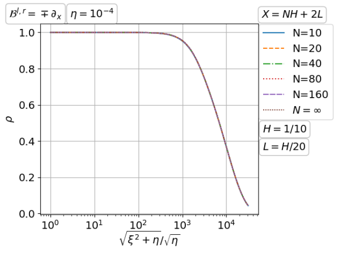
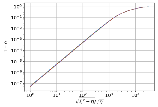
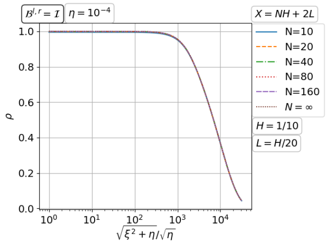
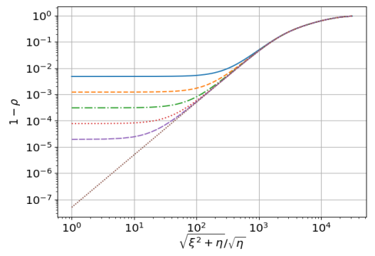
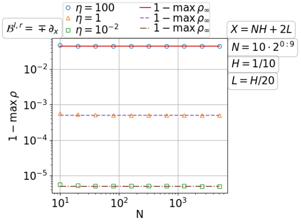
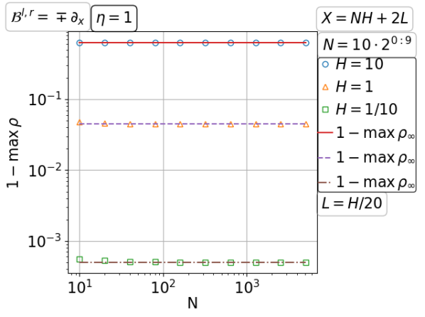
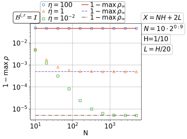
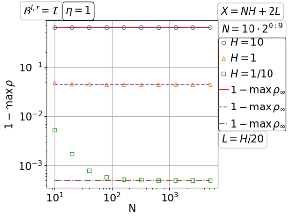
Figure 3.2: Convergence of the parallel Schwarz method with Dirichlet transmission for diffusion with increasing number of fixed size subdomains.

Convergence on a fixed domain with increasing number of subdomains

With the number of subdomains $N\to\infty$ and the domain width $X$ fixed, the results are shown in Figure 3.3 in a format similar to Figure 3.2. In this scaling, the symbol values $a$, $b$ vary with $N$ and no limiting spectral radius is known in closed form, since the matrix entries change with the scaling. But the plots of the convergence factor $\rho=\rho(\xi)$ in the left column of the top half of Figure 3.3 indicate the limiting curve is the constant one, and the plots in the right column display a constant slope in the $\log$ scale of $1-\rho$ for small $\sqrt{\xi^{2}+\eta}$. The slope is estimated to be $2$ for the Neumann problem and $0$ for the Dirichlet problem. The bottom half of Figure 3.3 shows the scaling $\max_{\xi}\rho=1-O(N^{-2})$ for various values of the coefficient $\eta$ and the overlap width $L$. The hidden constant factor in $O(N^{-2})$ can be seen depending linearly on $\eta$ and $\frac{L}{H}$ for the Neumann problem, and linearly on $\frac{L}{H}$ but is independent of small $\eta$ for the Dirichlet problem.

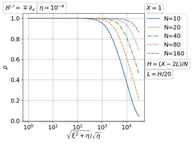
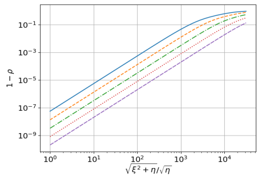
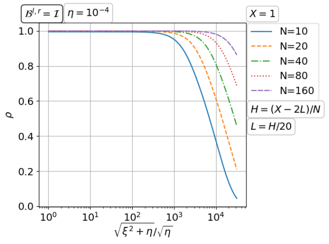
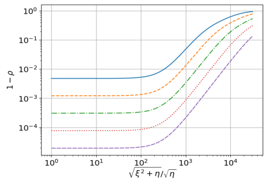
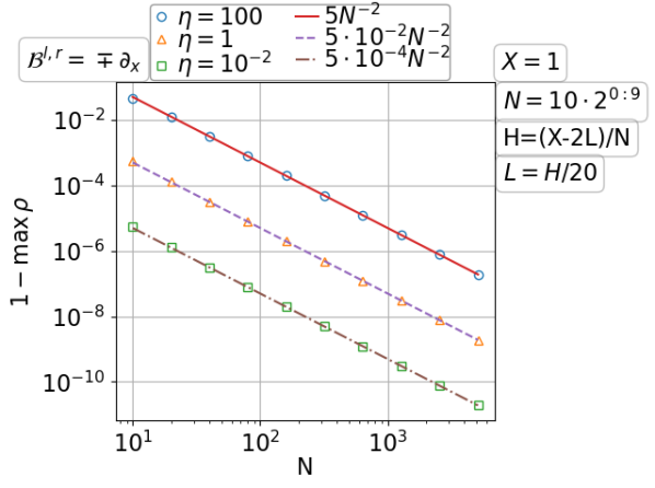
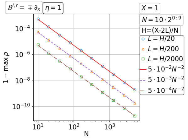
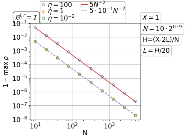
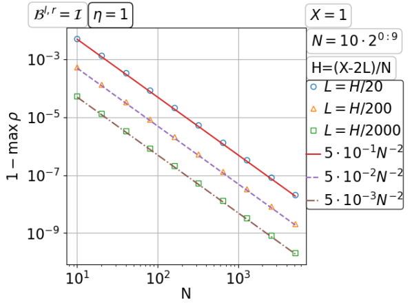
Figure 3.3: Convergence of the parallel Schwarz method with Dirichlet transmission for diffusion on a fixed domain with increasing number of subdomains.

Convergence with a fixed number of subdomains of shrinking width

With the number of subdomains $N$ fixed and the subdomain width $H\to 0$, we try to understand the dependence of the convergence factor $\rho$ on $H$ separately from the dependence on $N$. As we can see from the top half of Figure 3.4, smaller $H$ leads to slower convergence for all the Fourier frequencies $\xi$. Note that each graph of $\rho(\xi)$ for $N=10$ is accompanied with a graph of the corresponding $\rho_{\infty}$ for infinitely many subdomains $N=\infty$. So by “interpolation” one can imagine roughly the graphs for other values of $N$ based on the knowledge of Figure 3.2. In the right column of Figure 3.4, we see that, for the Neumann problem, the process of the subdomain width $H\to 0$ alone incurs the deterioration of convergence, while for the Dirichlet problem the process of $H\to 0$ needs to be combined with number of subdomains $N\to\infty$ to incur a deterioration. The bottom half of Figure 3.4 presents the scaling of $1-\max_{\xi}\rho$ with $H\to 0$. On the left for the overlap width $L=O(H)$, it shows that $\max_{\xi}\rho=1-O(H^{2})$ for the Neumann problem where $O(H^{2})$ depends linearly on the coefficient $\eta$, and $\max_{\xi}\rho=O(1)$ for the Dirichlet problem where $O(1)$ is independent of $\eta$. On the right, different values of $\nu$ for the overlap width $L=O({H^{\nu}})$ are used, which suggests $\max_{\xi}\rho=1-O(HL)$ for the Neumann problem and $\max_{\xi}\rho=1-O(H^{-1}L)$ for the Dirichlet problem.

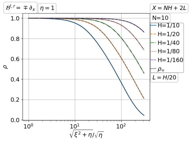
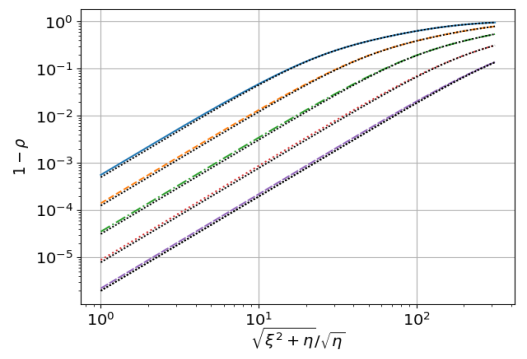
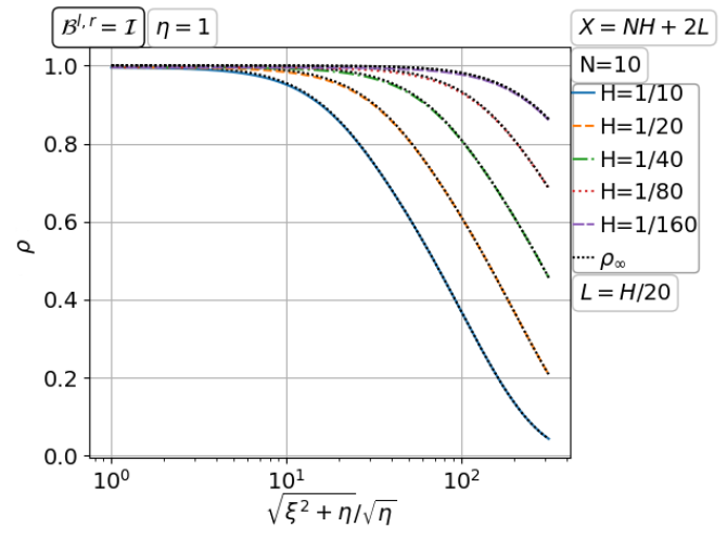
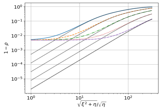
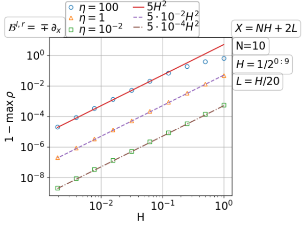
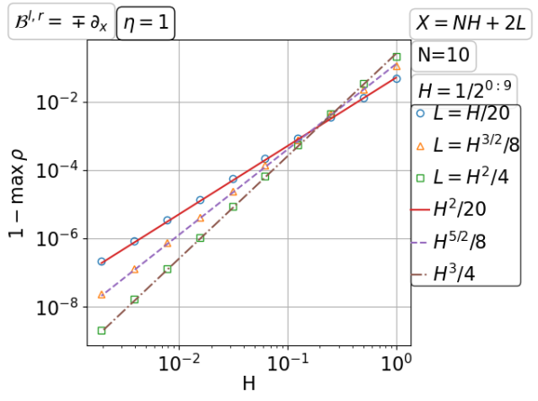
Figure 3.4: Convergence of the parallel Schwarz method with Dirichlet transmission for diffusion with a fixed number of subdomains of shrinking width.

Convergence on a fixed domain with a fixed number of subdomains of shrinking overlap

With both number of subdomains $N$ and the domain width $X$ fixed and the overlap width $L\to 0$, we find the convergence factor $\rho(\xi)\to 1$; see the top half of Figure 3.5. In particular, the right column shows a faster convergence of the Schwarz method for the Dirichlet problem than for the Neumann problem. The speed of $\max_{\xi}\rho=\rho(0)\to 1$ appears linear in $L\to 0$; see the bottom half of Figure 3.5. The hidden constant factor in $O(L)=1-\rho$ is $O(\eta H)$ for the Neumann problem and robust in the coefficient $\eta$ and subdomain width $H$ for the Dirichlet problem.

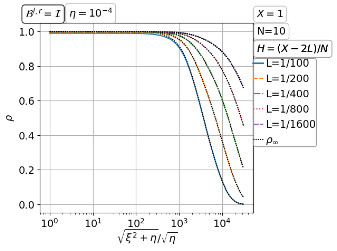
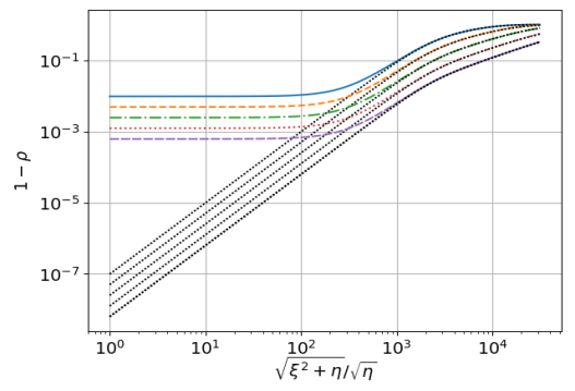
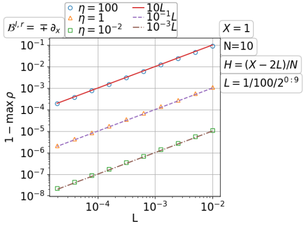
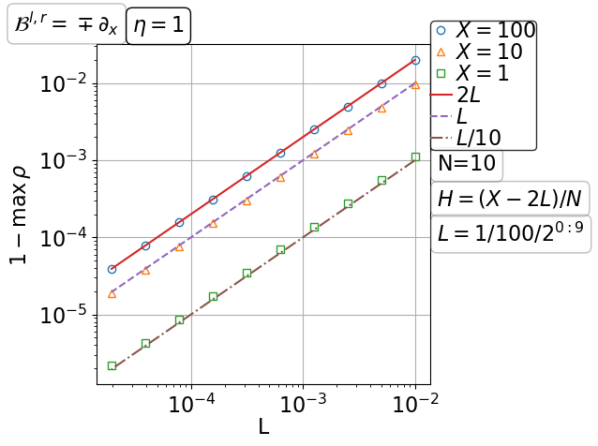
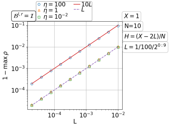
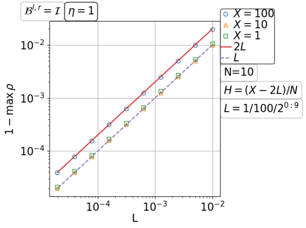
Figure 3.5: Convergence of the parallel Schwarz method with Dirichlet transmission for diffusion on a fixed domain with a fixed number of subdomains of shrinking overlap.

3.1.2 Parallel Schwarz method with Taylor of order zero transmission for the diffusion problem

By using the Taylor of order zero transmission condition, see Table 5, the subdomain problem away from the boundary $\{0,X\}\times[0,Y]$ is a domain truncation of the problem on the infinite pipe $(-\infty,\infty)\times[0,Y]$. It is interesting to check how the original boundary condtion on $\{0,X\}\times[0,Y]$ influences the convergence. At least, we expect the Schwarz method to work when the original boundary operator is also Taylor of order zero: $\mathcal{B}^{l,r}=\mathcal{B}^{l,r}_{j}$, because then the original problem is a domain trunction of the infinite pipe problem. In the following paragraphs, we will study the convergence of parallel Schwarz for the Dirichlet/Neumann/Taylor $\mathcal{B}^{l,r}$ separately. The literature on a general theory of the optimized Schwarz method with Robin transmission conditions is rather sparse. ? gave the first convergence proof in the non-overlapping case, without an estimate of the convergence rate, see also ?. It seems possible only at the discrete level to have a convergence rate of the non-overlapping optimized Schwarz method. ? got the first estimate of the convergence factor $1-O(h^{1/2}H^{-1/2})$ with an optimized choice of the Robin parameter; see also ?, ?, ?, ?, ?, ?, ?. In the overlapping case, the literature becomes even sparser, and there is only the work of ? to our knowledge.

Convergence with increasing number of fixed size subdomains

With the number of subdomains $N\to\infty$ and the subdomain width $H$, the overlap width $L$ fixed, two regimes can be observed in the top halves of Figure 3.6, 3.7, 3.8. In one regime, see the first row of each figure, the maximum point of the convergence factor $\rho(\xi)$ tends to $\xi=0$ as the number of subdomains $N\to\infty$. The other regime appears when the overlap width $L$ is sufficiently small, see the second row of each figure, in which the maximum point of $\rho(\xi)$ is almost fixed at the critical point of $\rho_{\infty}(\xi)=\lim_{N\to\infty}\rho(\xi)$. In both regimes, $\max_{\xi}\rho=O(1)<1$ as $N\to\infty$.

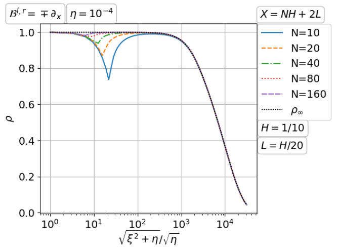
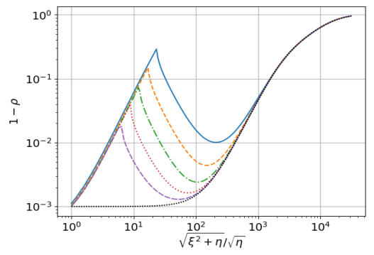
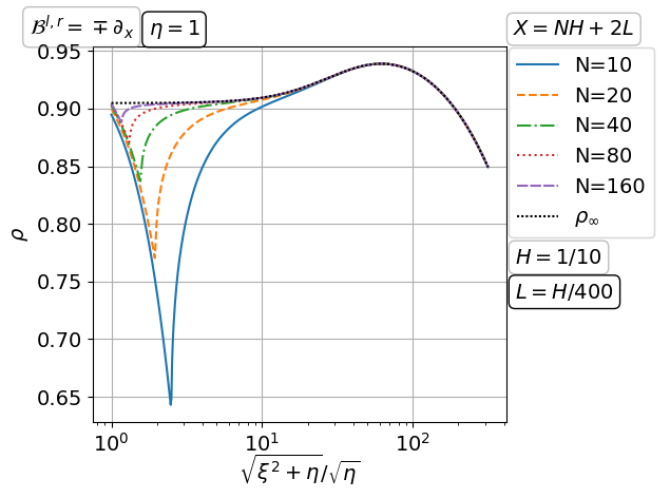
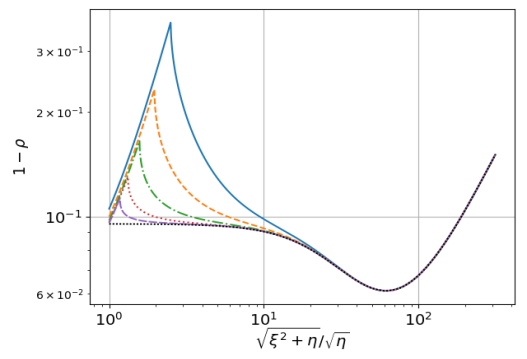
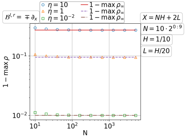
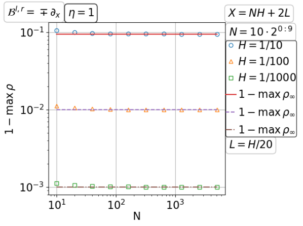
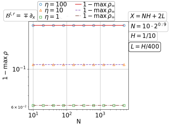
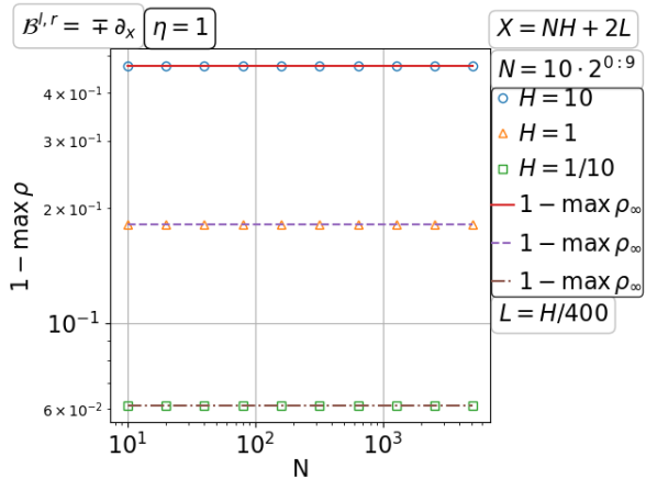
Figure 3.6: Convergence of the parallel Schwarz method with Taylor of order zero transmission for the Neumann problem of diffusion with increasing number of fixed size subdomains.

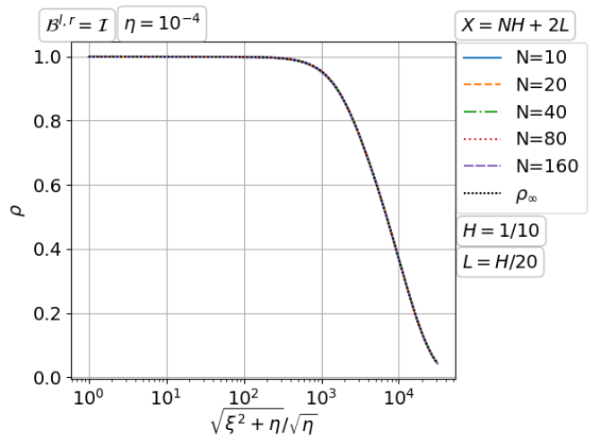
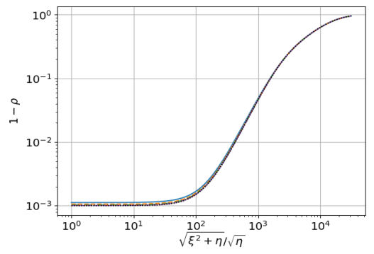
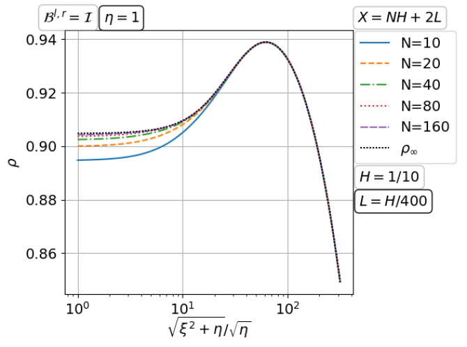
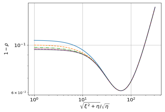
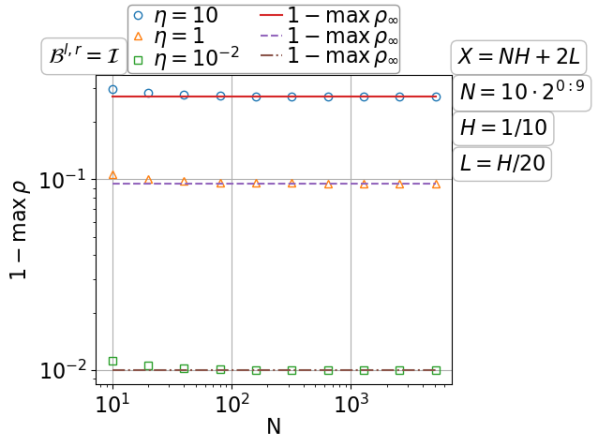
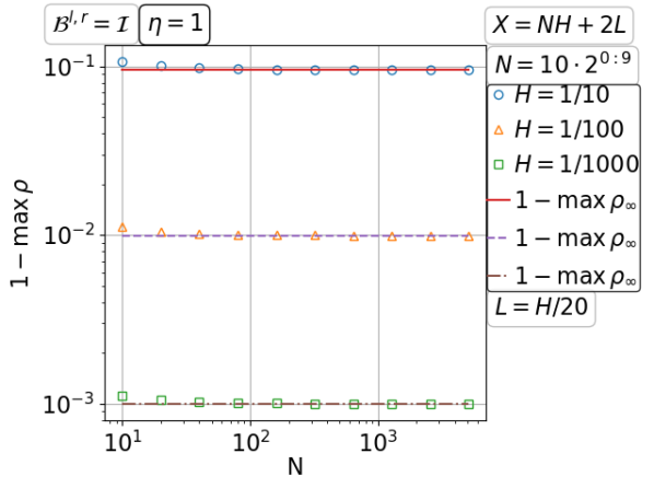
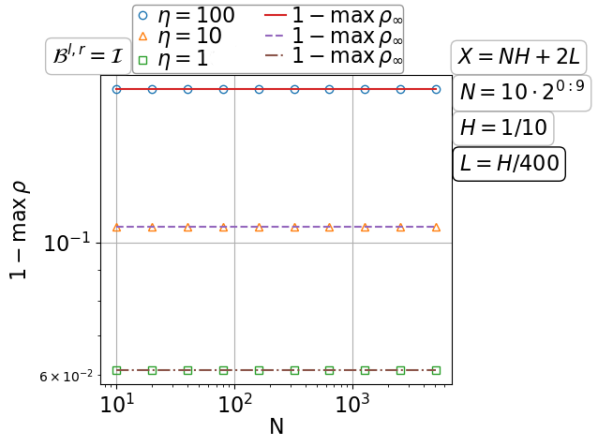
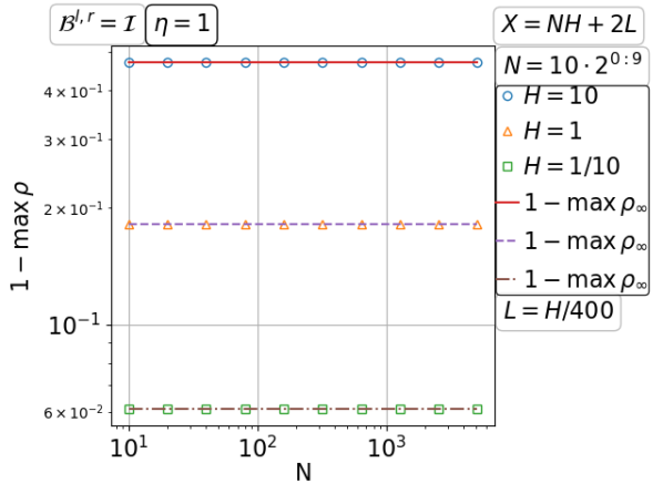
Figure 3.7: Convergence of the parallel Schwarz method with Taylor of order zero transmission for the Dirichlet problem of diffusion with increasing number of fixed size subdomains.

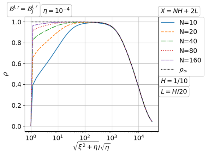
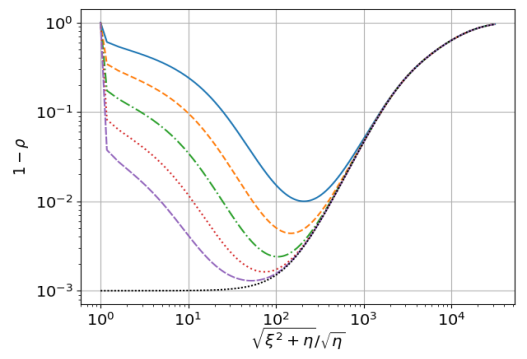
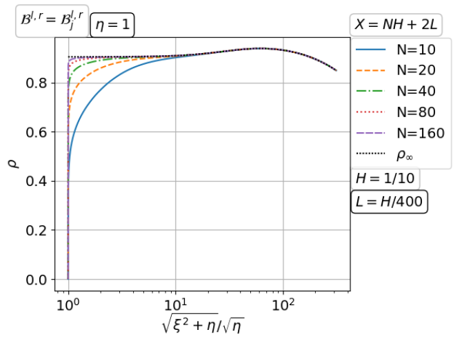
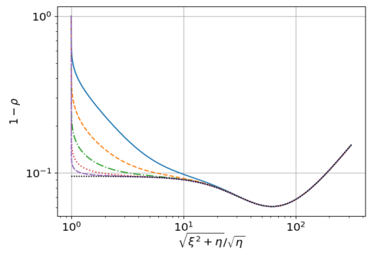
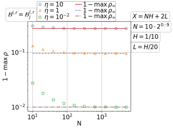
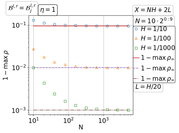
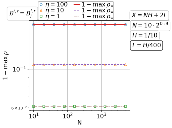
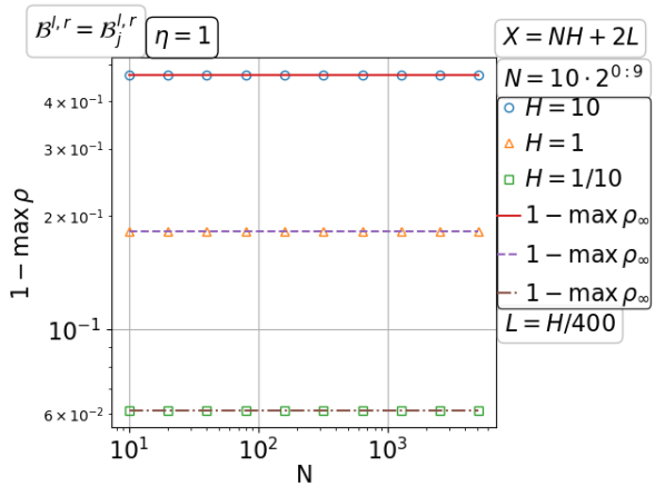
Figure 3.8: Convergence of the parallel Schwarz method with Taylor of order zero transmission for the infinite pipe diffusion with increasing number of fixed size subdomains.

Convergence on a fixed domain with increasing number of subdomains

With the number of subdomains $N\to\infty$ and the domain width $X$ fixed, it follows that the subdomain width $H\to 0$. The convergence for the Neumann problem is studied in Figure 3.9. Recall that $\rho_{\infty}:=\lim_{N\to\infty}\rho$ for fixed $H$, $L$ but $X=NH+2L$. From the top half of Figure 3.9, we find that the convergence factor $\rho(\xi)$ attains its maximum at $\xi=0$ when the overlap width $L=O(H)$ is not too small and at the critical point of $\rho_{\infty}(\xi)$ when $L=O(H^{2})$ is sufficiently small. In both regimes, it holds that $\max_{\xi}\rho=1-O(N^{-1})$. The difference is in how the hidden factor depends on $\eta$ and $L$: in the first regime $\max_{\xi}\rho=1-O(\sqrt{\eta}N^{-1})$ independent of $L$, while in the latter regime $\max_{\xi}\rho=1-O(\eta^{1/4}\sqrt{L}N^{-1})$. Note that we have the same (up to a constant factor) dependence on $L$ and $\eta$ as in TaylorRho from the two-subdomain analysis. The convergence for the Dirichlet problem and the infinite pipe problem are studied in Figure 3.10 and Figure 3.11. Albeit the graphs of $\rho$ look different, the maximum of $\rho$ depends on $N$ in the same way as for the Neumann problem.

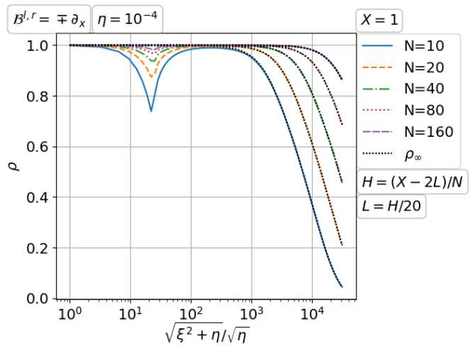
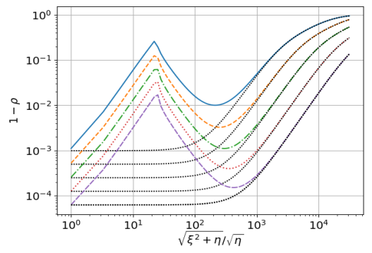
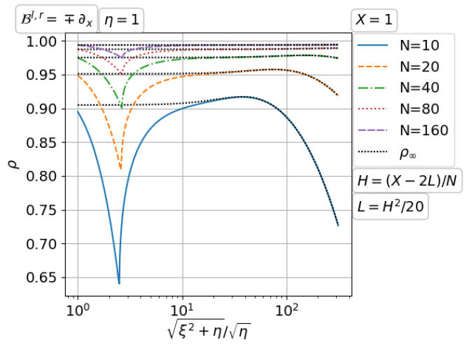
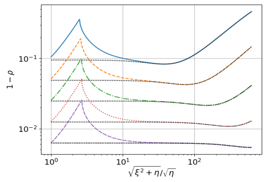
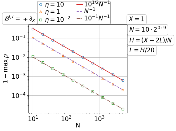
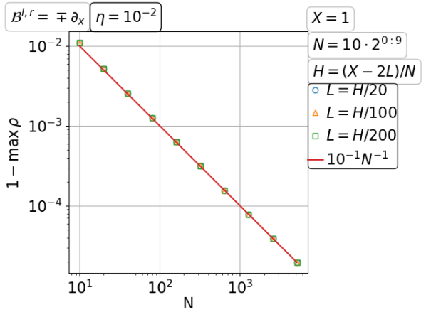
Figure 3.9: Convergence of the parallel Schwarz method with Taylor of order zero transmission for the Neumann problem of diffusion on a fixed domain with increasing number of subdomains.

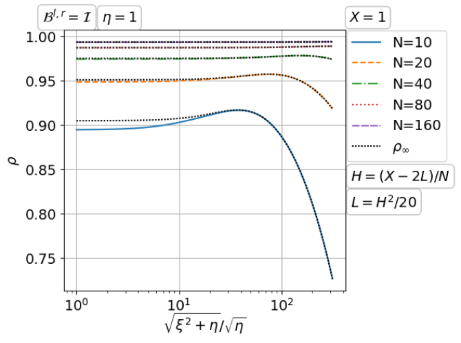
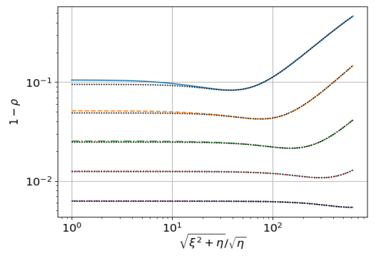
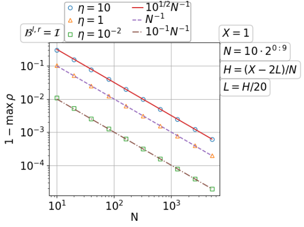
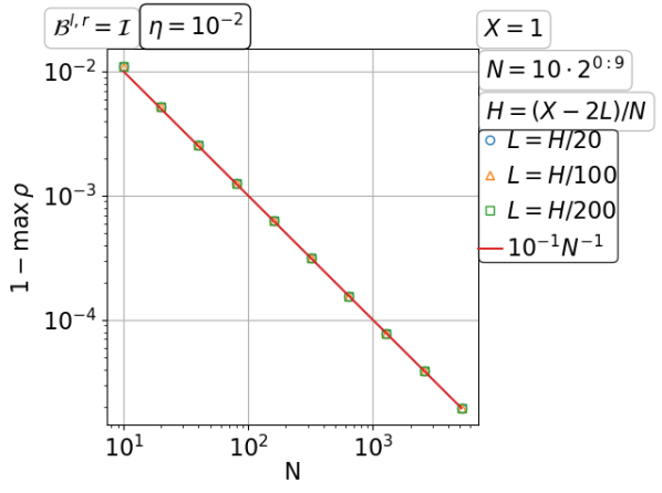
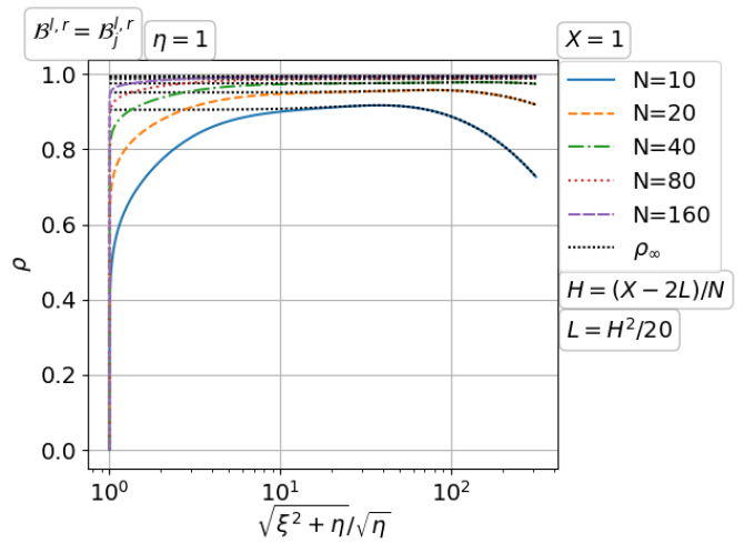
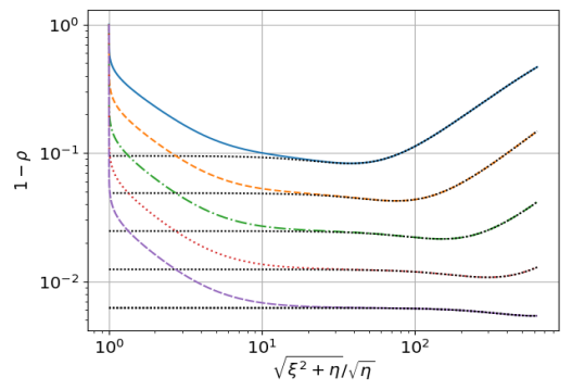
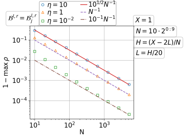
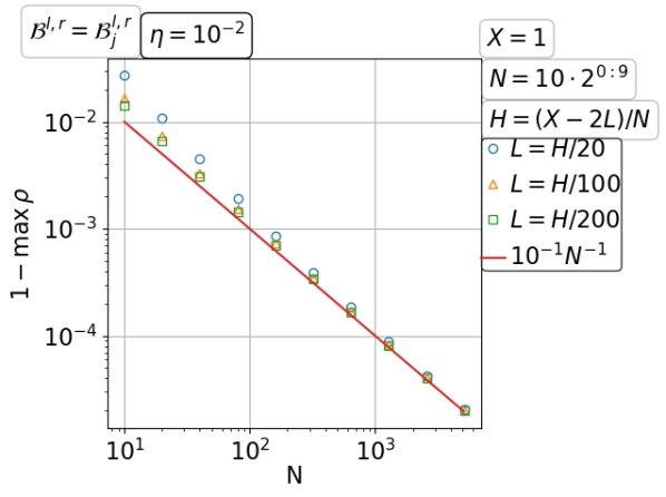
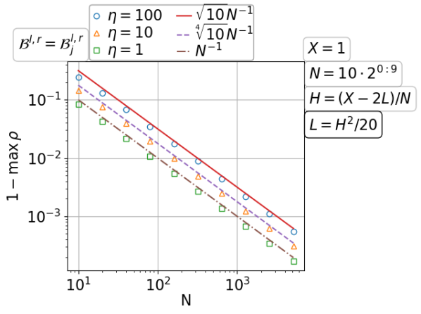
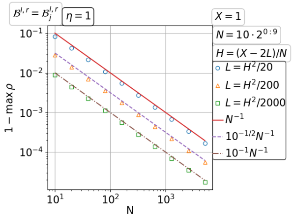
Figure 3.10: Convergence of the parallel Schwarz method with Taylor of order zero transmission for the Dirichlet problem of diffusion on a fixed domain with increasing number of subdomains.

Figure 3.11: Convergence of the parallel Schwarz method with Taylor of order zero transmission for the infinite pipe diffusion on a fixed domain with increasing number of subdomains.

3.1.3 Parallel Schwarz method with PML transmission for the diffusion problem

By using the PML transmission condition, the subdomain problem away from the boundary $\{0,X\}\times[0,Y]$ can be a very good domain truncation of the problem on the infinite pipe $(-\infty,\infty)\times[0,Y]$, because PML can make the reflection coefficient

$$R=\frac{\hat{\mathcal{S}}-\sqrt{\xi^{2}+\eta}}{\hat{\mathcal{S}}+\sqrt{\xi^{2}+\eta}}=\pm\mathrm{e}^{-(2+\gamma)D\sqrt{\xi^{2}+\eta}}\qquad\text{($\hat{\mathcal{S}}$ given in \R{eqhats})}$$

arbitrarily small by increasing its numerical cost related to the PML width $D$ and PML strength $\gamma$. If the original boundary condition is also given by PML, i.e., $\mathcal{B}^{l,r}=\mathcal{B}^{l,r}_{j}$, then the original problem does approximate the infinite pipe problem and so we can expect that the Schwarz method will perform well. What if $\mathcal{B}^{l,r}$ is Dirichlet or Neumann? What condition should be used on the external boundary of the PML? We will address these questions in the following paragraphs.

Convergence with increasing number of fixed size subdomains

The study is carried out on a growing chain of fixed size subdomains. We first consider the Neumann problem in Figure 3.12. The first row is the convergence factor $\rho(\xi)$ from using the Neumann condition on the PML external boundaries, while the second row is from using the Dirichlet condition. We see that their asymptotics $\rho_{\infty}(\xi)=\lim_{N\to\infty}\rho(\xi)$ have little difference but the Neumann terminated PML is better than the Dirichlet terminated PML for moderate number of subdomains $N$, which is reasonable because the original domain $\Omega$ is equipped with the Neumann condition. In the bottom half of Figure 3.12, we see that $\max_{\xi}\rho=O(1)<1$ with the constant linearly dependent on the coefficient $\eta$ and the PML width $D$. If we compare this figure with Figure 3.2 and Figure 3.5, we can find many similarities. That is, the PML for diffusion behaves like an overlap (see also patch substructuring methods (?), and references therein). But the PML can be of arbitrary width, while the overlap width can not exceed the subdomain width. The same scaling is observed for the Dirichlet problem in Figure 3.13 and for the truncated infinite pipe problem in Figure 3.14. For a moderate number of subdomains, the Dirichlet terminated PML is favorable for the original Dirichlet problem.

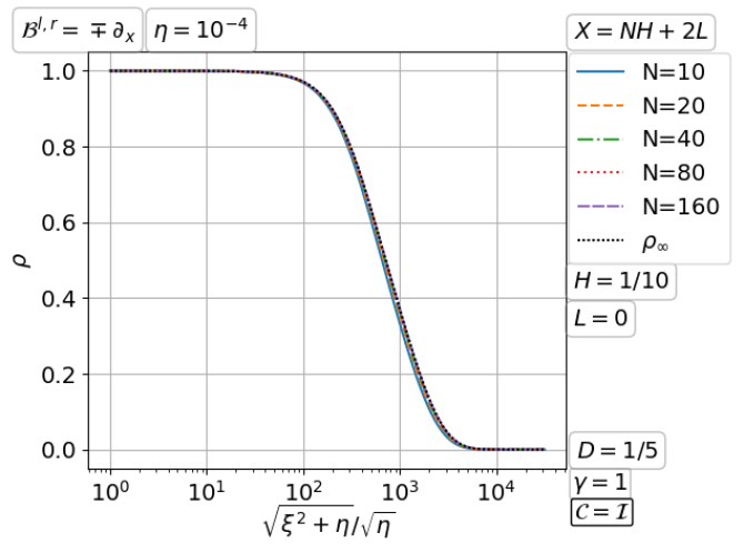
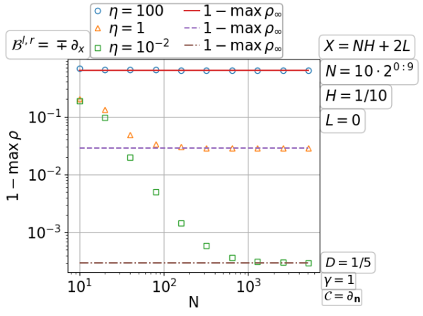
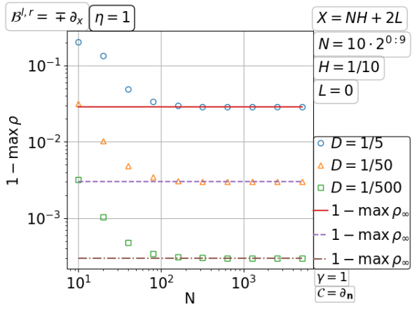
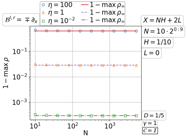
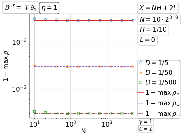
Figure 3.12: Convergence of the parallel Schwarz method with PML transmission for the Neumann problem of diffusion with increasing number of fixed size subdomains.

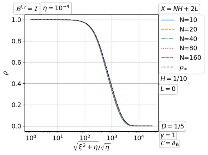
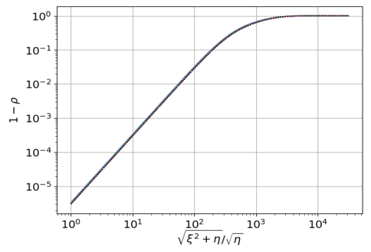
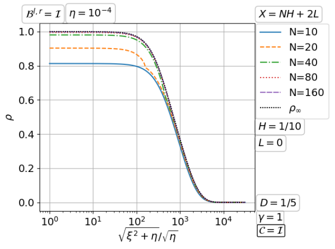
Figure 3.13: Convergence of the parallel Schwarz method with PML transmission for the Dirichlet problem of diffusion with increasing number of fixed size subdomains.

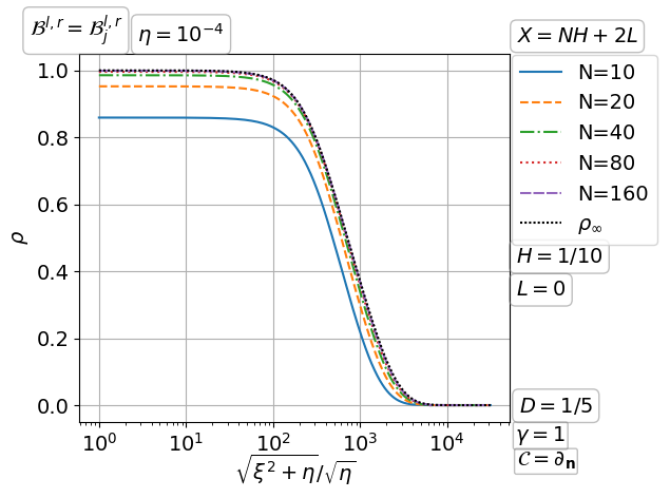
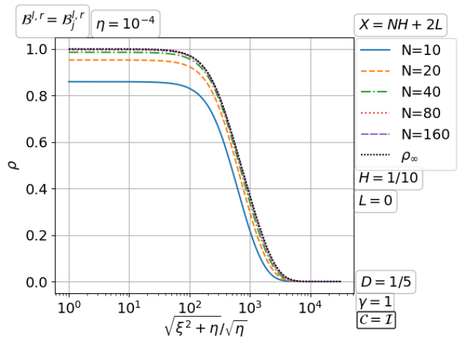
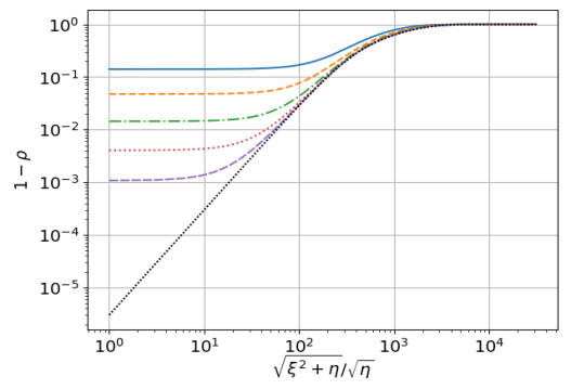
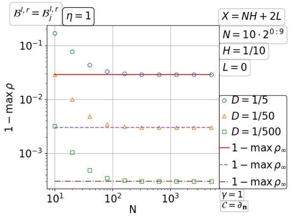
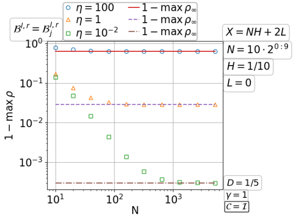
Figure 3.14: Convergence of the parallel Schwarz method with PML transmission for the infinite pipe diffusion with increasing number of fixed size subdomains.

Convergence on a fixed domain with increasing number of subdomains

In this scaling, the subdomain width $H=(X-2L)/N\to 0$ as the number of subdomains $N\to\infty$ and the domain width $X$ is fixed. Different from the overlap width $L$, the PML width $D$ is not bound to $H$ and so it can be fixed. From the top half of Figure 3.15, we can find that $\rho_{\infty}=\lim_{N\to\infty}\rho$ (the limit taken for each fixed $H$) is tending to the constant one as $H\to 0$ and the change of $1-\rho$ with growing $N$ looks the same as the change of $1-\rho_{\infty}$. The convergence deterioration is estimated in the bottom half of Figure 3.15 as $1-\max_{\xi}\rho=O(N^{-1})$ with a linear dependence on the PML width $D$. The condition on the external boundary of the PML plays a significant role for small $\eta>0$; see the first column of the bottom half of Figure 3.15. If the PML is terminated with the same condition as for the original domain, i.e., $\mathcal{C}=\mathcal{B}^{l,r}$, then $1-\max_{\xi}\rho$ tends to be robust for small $\eta>0$; otherwise, the convergence deteriorates with $\eta\to 0^{+}$. A similar phenomenon appears for the classical Dirichlet transmission, see the earlier Figure 3.3, in particular, the first column of the bottom half. All the above observations apply equally to the Dirichlet problem (Figure 3.16) and the infinite pipe problem (Figure 3.17).

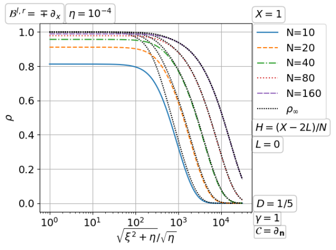
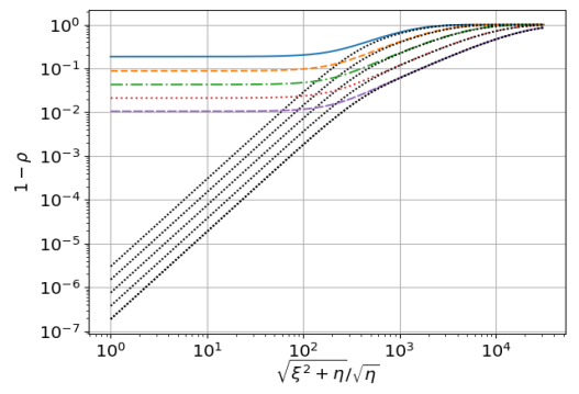
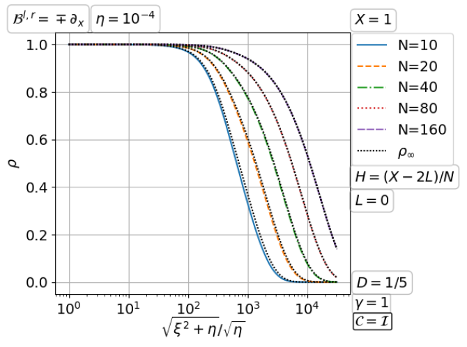
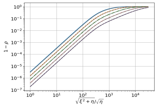
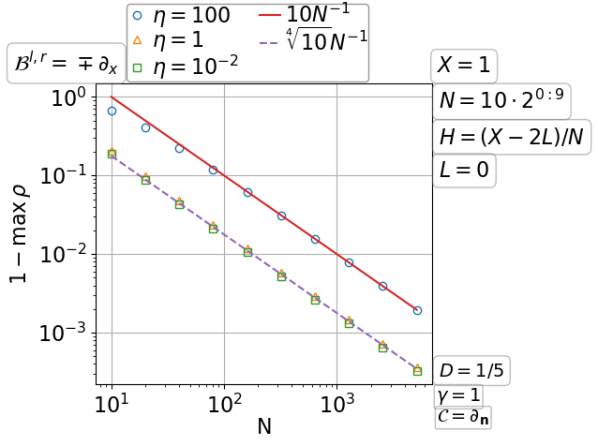
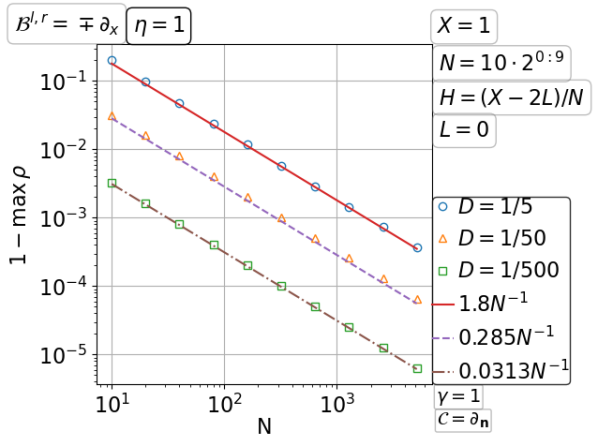
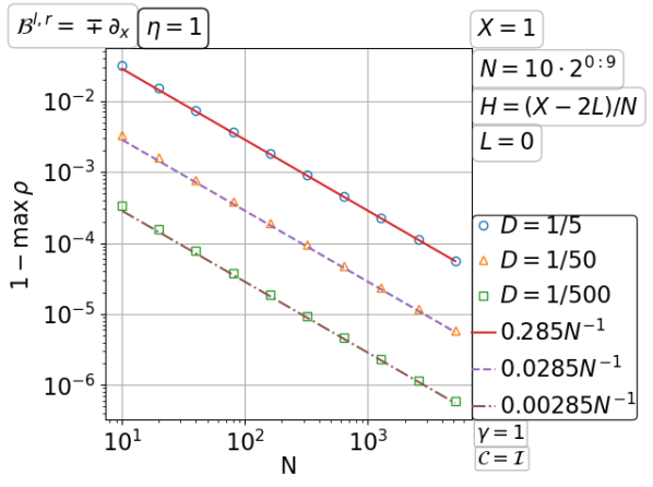
Figure 3.15: Convergence of the parallel Schwarz method with PML transmission for the Neumann problem of diffusion on a fixed domain with increasing number of subdomains.

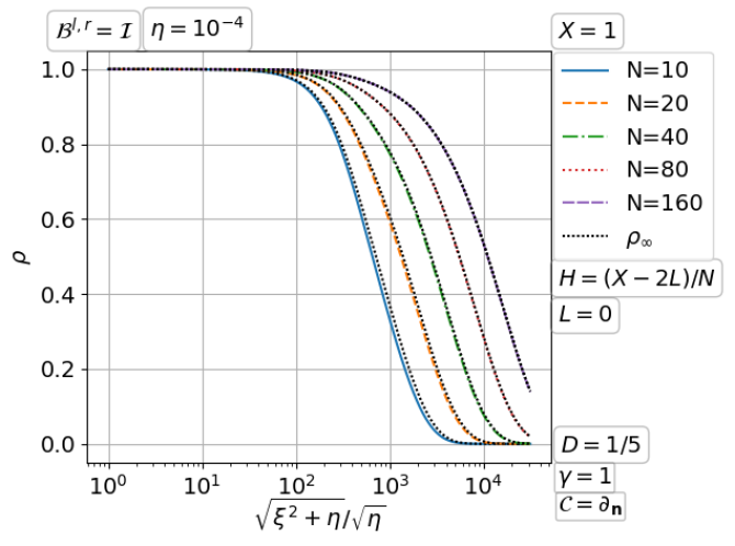
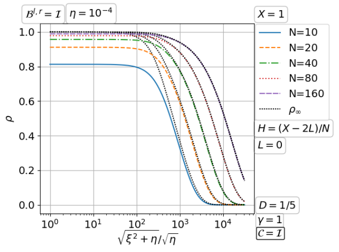
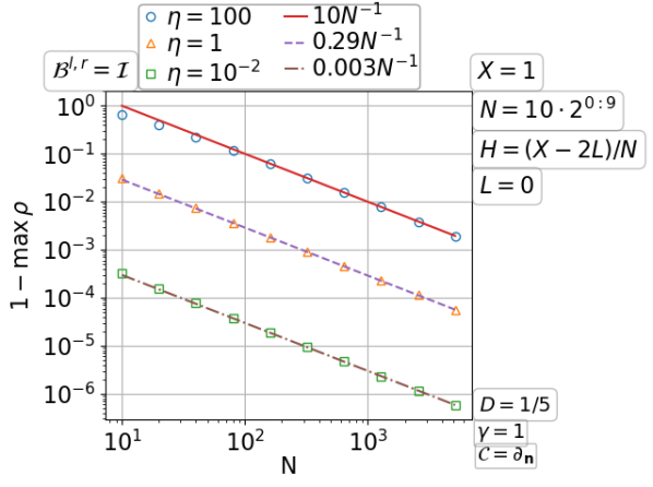
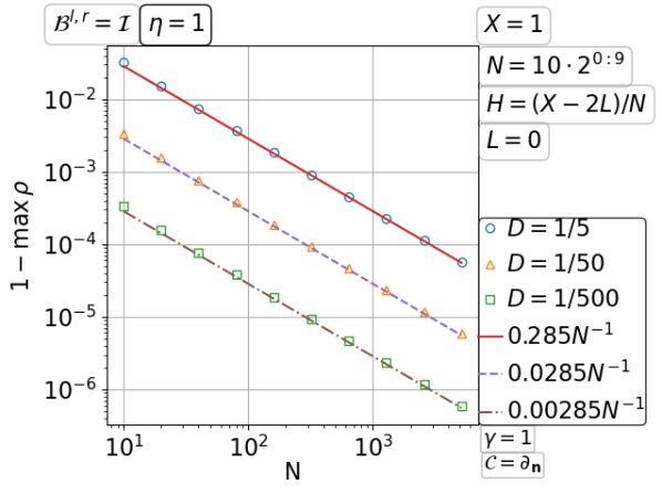
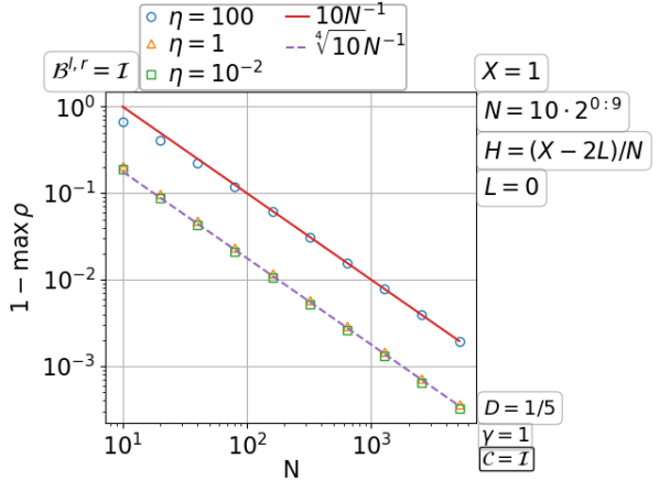
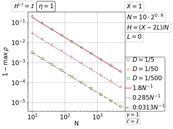
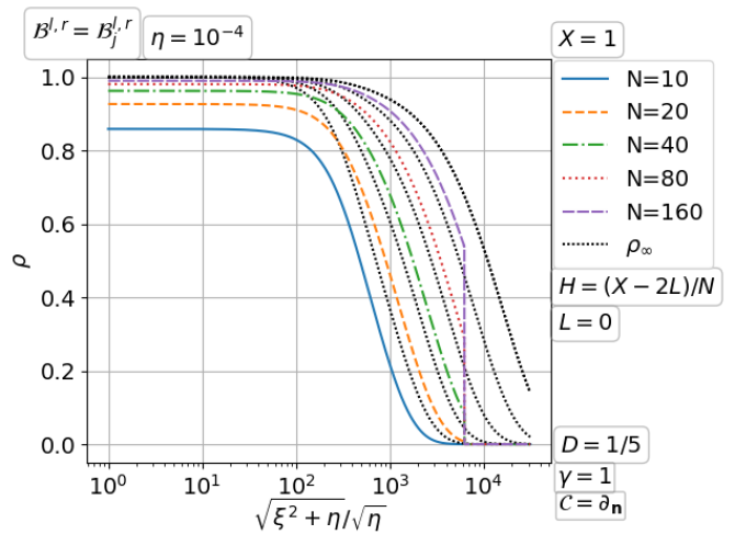
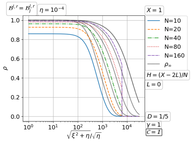
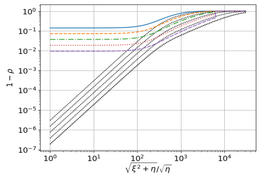
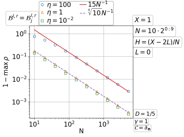
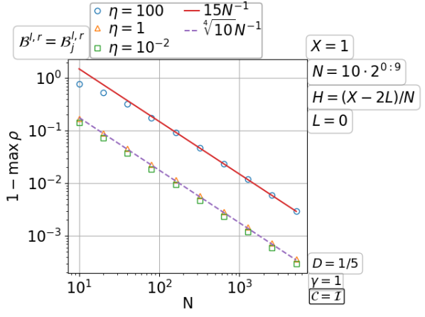
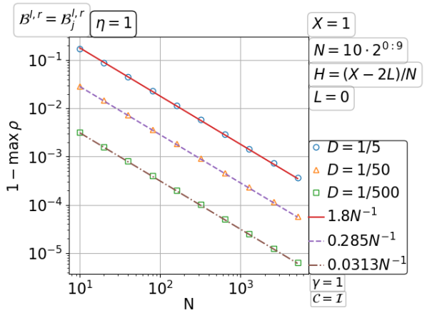
Figure 3.16: Convergence of the parallel Schwarz method with PML transmission for the Dirichlet problem of diffusion on a fixed domain with increasing number of subdomains.

Figure 3.17: Convergence of the parallel Schwarz method with PML transmission for the infinite pipe diffusion on a fixed domain with increasing number of subdomains.

3.2 Double sweep Schwarz methods for the diffusion problem

Double sweep Schwarz methods differ from parallel Schwarz methods in the order of updating subdomain solutions, which is analogous to the difference between the symmetric Gauss-Seidel and Jacobi iterations. Moreover, the block symmetric Gauss-Seidel method and the block Jacobi method are special double sweep and parallel Schwarz methods with minimal overlap and Dirichlet transmission condition. On the one hand, it is typical that the Gauss-Seidel iteration (sweep in only one order of the unknowns) converges twice as fast as the Jacobi iteration, and the symmetric Gauss-Seidel method is no more than twice as fast as the Gauss-Seidel method; see e.g. ?. On the other hand, the optimal double sweep Schwarz method converges in one iteration, much faster than the optimal parallel Schwarz method that converges in $N$ iterations. Of course, it comes at a price: the double sweep is inherently sequential between subdomains, while the parallel Schwarz method allows all the subdomain problems to be solved simultaneously in one iteration. Our goal in this subsection is to investigate the convergence speed in the general setting between these two limits.

3.2.1 Double sweep Schwarz method with Dirichlet transmission for the diffusion problem

The method proposed by ? uses Dirichlet transmission conditions and overlap. It solves the subdomain problems in alternating order, now also known as double sweep (?). At the matrix level, the classical Schwarz method can be viewed as an improvement of the block symmetric Gauss-Seidel method by adding overlaps between blocks. So, yet another name for the double sweep Schwarz method is the symmetric multiplicative Schwarz method (?, Section 1.6). It can be seen from ? that the convergence factor of the method is bounded from above by $1-O(H^{2})$ for an overlap $L=O(H)$. In the classical context with Dirichlet transmission, the symmetric multiplicative Schwarz method is rarely used because there would be no benefit in convergence (?) compared to the (single sweep) multiplicative Schwarz method.

Convergence with increasing number of fixed size subdomains

In the top half of Figure 3.18, the convergence factor $\rho(\xi)$ of the double sweep Schwarz method is shown for growing $N$ (number of subdomains). There seems to be a limiting curve $\rho_{\infty}:=\lim_{N\to\infty}\rho$ independent of the original boundary condition on $\{0,X\}\times[0,Y]$. From the bottom half of Figure 3.18, the scaling of the double sweep iteration turns out to be $1-\max_{\xi}\rho=O(1)\in(0,1)$ with a linear dependence on the overlap width $L$. The dependence on the coefficient $\eta>0$ is linear for both Neumann and Dirichlet problems. Comparing with the parallel iteration studied in Figure 3.2, the double sweep iteration shown in Figure 3.18 does converge faster. More precisely, comparing the botttom left quandrants of the two figures, we find the double sweep iteration is about twice as fast as the parallel iteration.

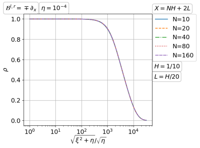
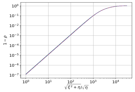
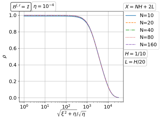
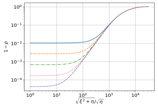
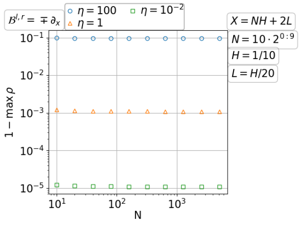
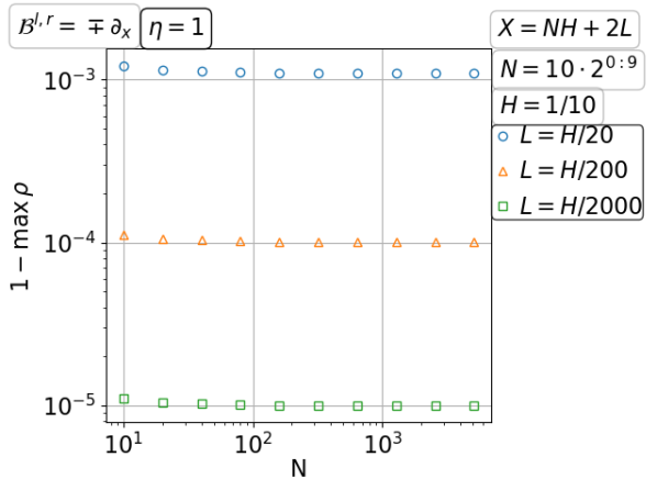
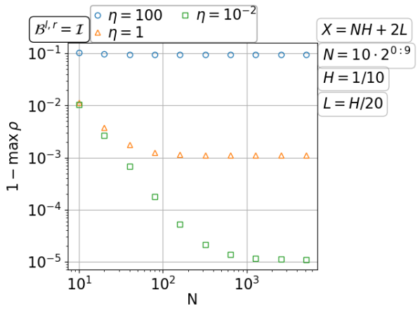
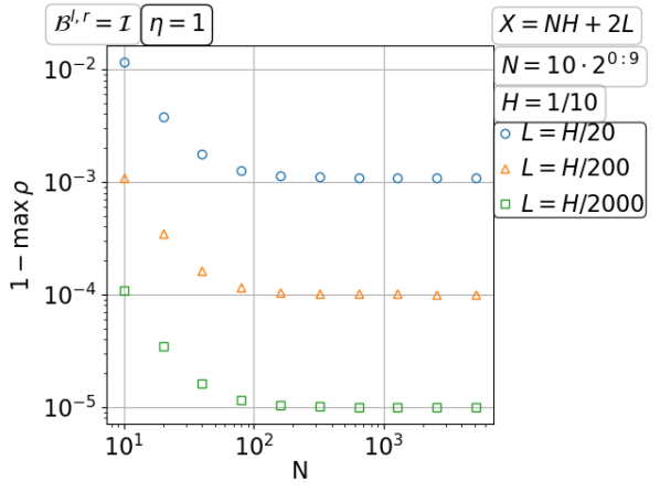
Figure 3.18: Convergence of the double sweep Schwarz method with Dirichlet transmission for diffusion with increasing number of fixed size subdomains.

Convergence on a fixed domain with increasing number of subdomains

We find from the top half of Figure 3.19 that the graph of the convergence factor $\rho(\xi)$ for the double sweep Schwarz method tends to the constant $1$ when we refine the decomposition on a fixed domain. For small $\eta>0$, the convergence is much faster for the Dirichlet problem than for the Neumann problem, a phenomenon observed also with the parallel Schwarz method in Figure 3.3. The scaling of $\max_{\xi}\rho(\xi)=\rho(0)$ is illustrated in the bottom half of Figure 3.19. Note that a large overlap $L=O(H)$ is considered. We find $\max_{\xi}\rho=1-O(N^{-2})$, the same as of the parallel Schwarz method shown in Figure 3.3. The dependence on the coefficient $\eta>0$ and the overlap width $L$ is also the same as before. A more careful comparison of the two figures shows that the double sweep iteration is about twice as fast as the parallel iteration.

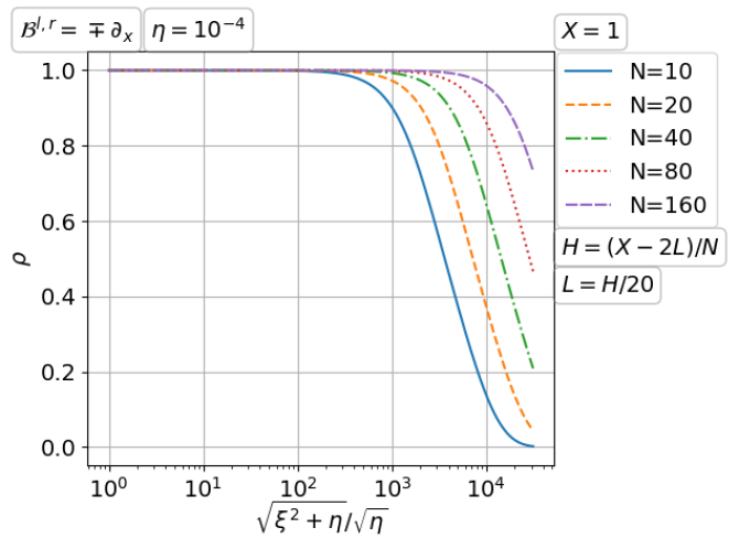
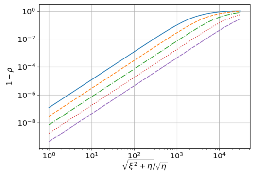
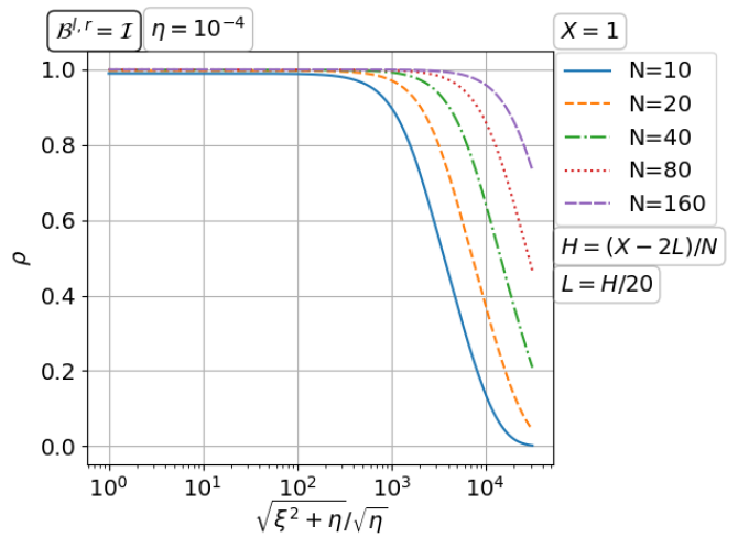
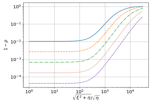
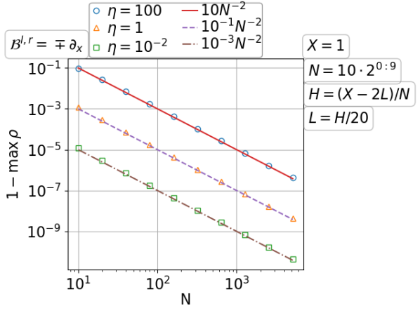
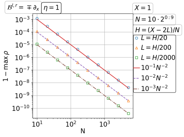
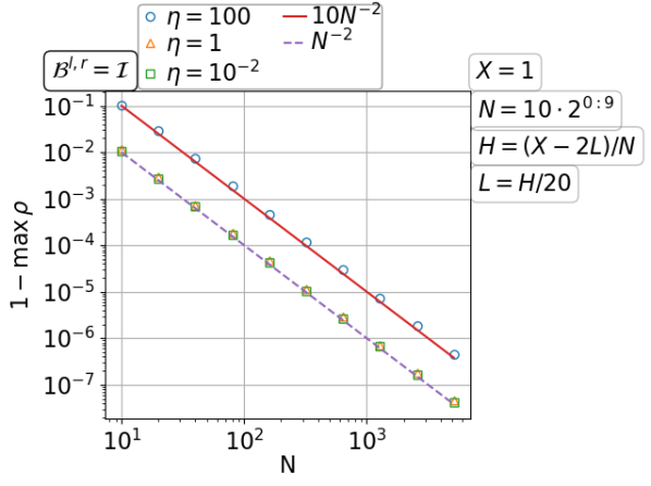
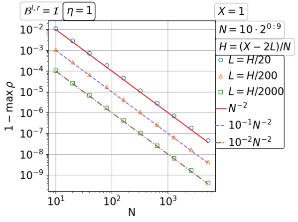
Figure 3.19: Convergence of the double sweep Schwarz method with Dirichlet transmission for diffusion on a fixed domain with increasing number of subdomains.

3.2.2 Double sweep Schwarz method with Taylor of order zero transmission for the diffusion problem

The Taylor of order zero condition is designed for domain truncation of unbounded problems. It is interesting to see how such transmission conditions work for other problems. As we did for the parallel Schwarz method, three types of boundary value problems – the Dirichlet, Neumann and infinite pipe problems will all be investigated. Another important goal is to find out how much is gained from the parallel iteration to the double sweep iteration.

Convergence with increasing number of fixed size subdomains

For the double sweep Schwarz method, there also seems to be a limiting curve $\rho_{\infty}=\lim_{N\to\infty}\rho$ independent of the boundary condition defined by $\mathcal{B}^{l,r}$; see Figure 3.20. The maximum of $\rho$ is attained at an asymptotic point away from $\xi=0$ as $N\to\infty$. Since the scaling is found independent of $\mathcal{B}^{l,r}$, only one boundary condition is illustrated; see the bottom row of Figure 3.20. The observation is $\rho=O(1)<1$ with a square-root dependence on the overlap width $L$. Compared to the subplot in the third row and first column of Figure 3.7, the double sweep iteration is three to four times as fast as the parallel iteration.

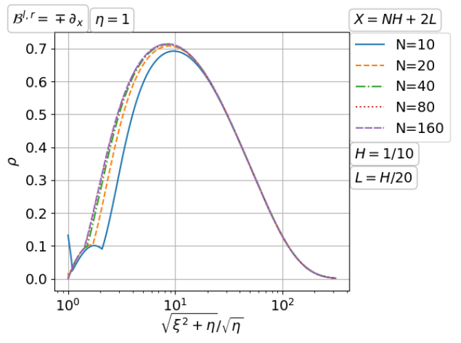
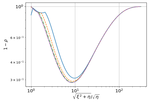
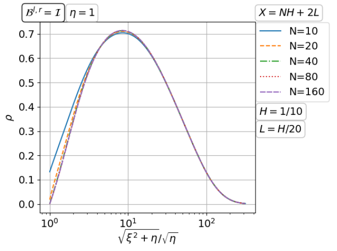
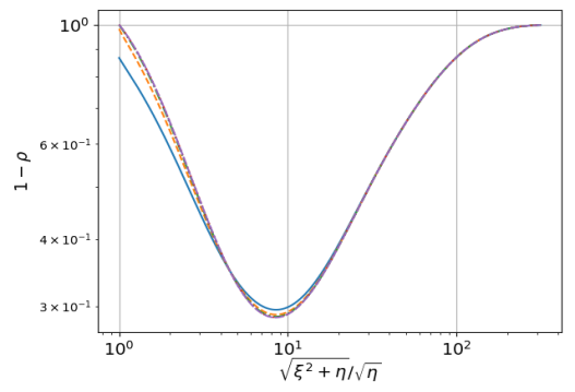
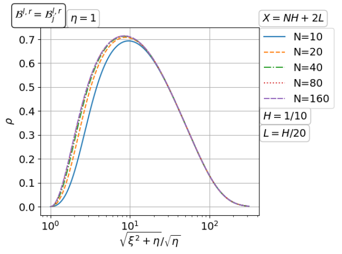
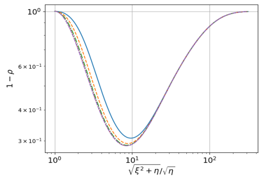
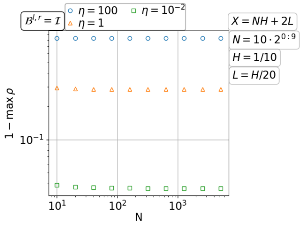
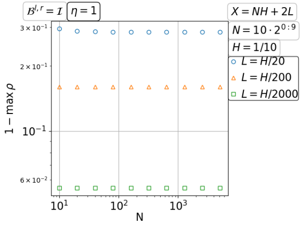
Figure 3.20: Convergence of the double sweep Schwarz method with Taylor of order zero transmission for diffusion with increasing number of fixed size subdomains.

Convergence on a fixed domain with increasing number of subdomains

In the first three rows of Figure 3.21, we see a deterioration of the convergence as we refine the decomposition of a fixed domain: a peak of the convergence factor $\rho$ rises and expands to the right to form a plateau. The shape and location of the plateu are almost the same for the three types of boundary value problems. Clearly, the double sweep Schwarz method is not a smoother. The scaling of $\max_{\xi}\rho$ is illustrated in the bottom row of Figure 3.21 for the Dirichlet problem. We find $\max_{\xi}\rho=1-O(N^{-1})$. The hidden constant factor in $O(N^{-1})$ has a square-root dependence on the coefficient $\eta>0$ and a mild dependence on the overlap width $L\to 0^{+}$. Compared to the parallel iteration explored in Figure 3.10, the double sweep iteration scales the same way but converges $3\sim 4$ times as fast.

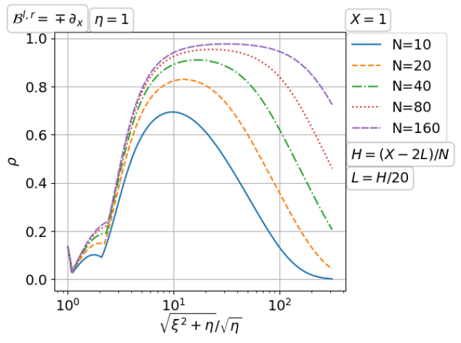
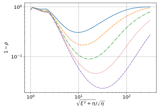
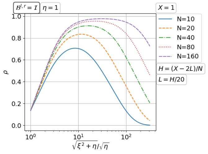
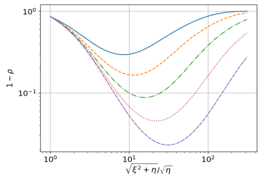
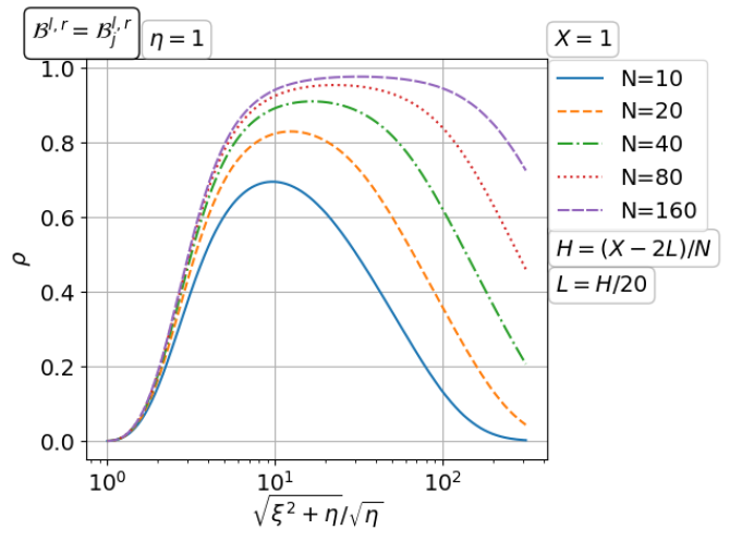
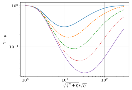
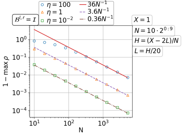
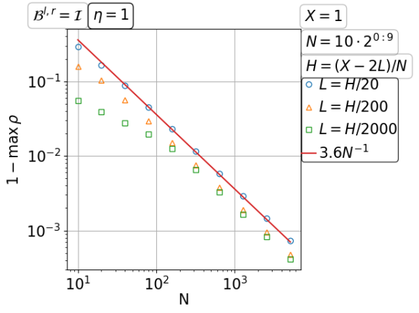
Figure 3.21: Convergence of the double sweep Schwarz method with Taylor of order zero transmission for diffusion on a fixed domain with increasing number of subdomains.

3.2.3 Double sweep Schwarz method with PML transmission for the diffusion problem

So far, the transmission conditions that we have explored for the double sweep Schwarz methods are the Dirichlet and Taylor of order zero conditions, which both rely on the overlap width $L>0$ to control the high frequency error. Compared to their parallel Schwarz counterparts, these double sweep Schwarz methods do not improve the scaling orders in $N$ (number of subdomains) but only the constant factors. Will the comparison carry over to the PML condition? For the parallel Schwarz methods on a fixed domain, we have seen that a fixed PML condition leads to the convergence rate $\max_{\xi}\rho=1-O(N^{-1})$, the same as the Taylor of order zero condition does, which is not strange given that the optimal parallel Schwarz method converges in $N$ iterations. But the optimal double sweep Schwarz method converges in just one iteration. So, if a double sweep Schwarz method deteriorates with growing $N$, then we can owe the deterioration to the non-optimal transmission condition, e.g., the Taylor of order zero condition. Can the PML condition as a more accurate domain truncation technique push the double sweep Schwarz method toward the optimal one? How good a PML in terms of the PML width $D$ and strength $\gamma$ do we need to achieve the constant scaling independent of $N$? Let us find out the answers below.

Convergence with increasing number of fixed size subdomains

Three types of boundary value problems – Neumann, Dirichlet and infinite pipe problems are explored in individual figures; see Figure 3.22, Figure 3.23 and Figure 3.24. In each case, we test both the Dirichlet and Neumann terminating conditions for the PML. For example, in Figure 3.22, the first row is for the Neumann terminated PML and the second row is for the Dirichlet terminated PML. We see as $N\to\infty$, the graph of $\rho(\xi)$ tends to some limiting profile, independent of the PML terminating condition and the original boundary condition. The existence of $\lim_{N\to\infty}\rho<1$ implies the scaling $\max_{\xi}\rho(\xi)=\rho(0)=O(1)<1$ for all $N$, which is confirmed with scaling plots in the bottom halves of the figures. For moderate $N$, we find it better to use the same condition as for the original problem to terminate the PML. As expected, the convergence rate improves for bigger PML width $D$ but deteriorates for smaller coefficient $\eta>0$. Compared to the parallel Schwarz method shown in Figure 3.12, Figure 3.13 and Figure 3.14, the double sweep method is about $10$ times as fast.

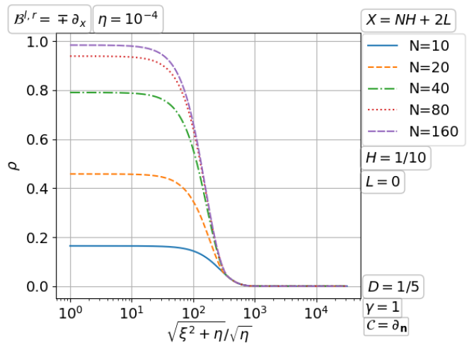
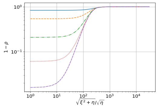
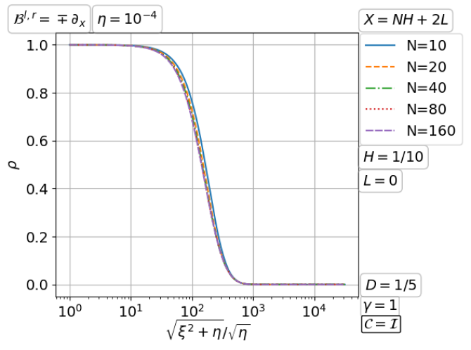
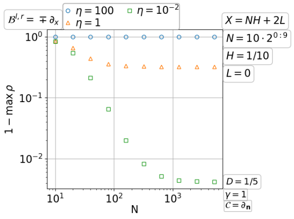
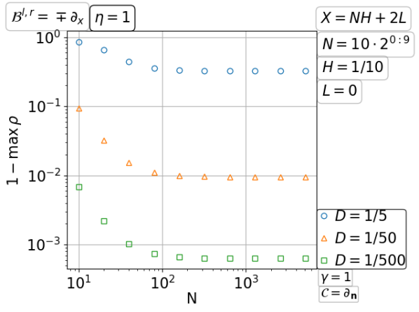
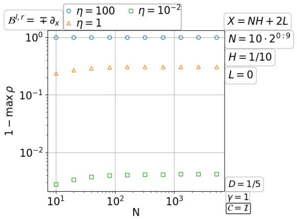
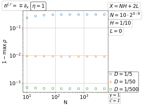
Figure 3.22: Convergence of the double sweep Schwarz method with PML transmission for the Neumann problem of diffusion with increasing number of fixed size subdomains.

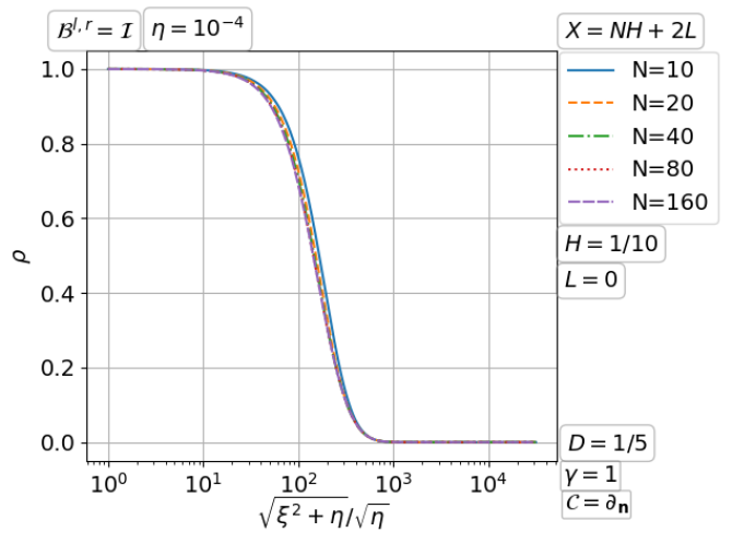
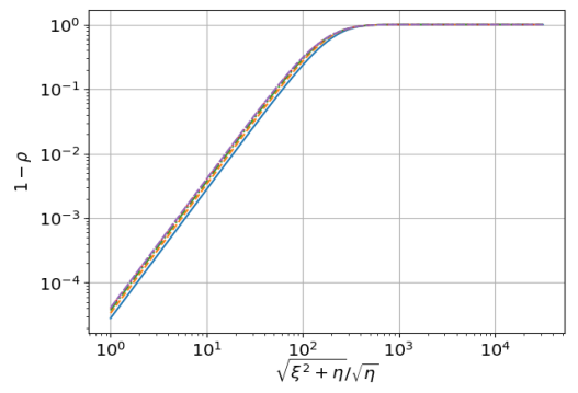
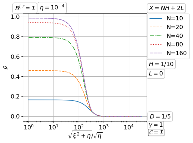
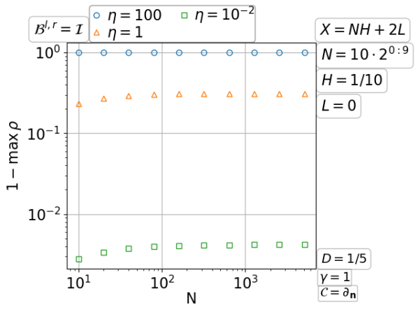
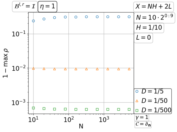
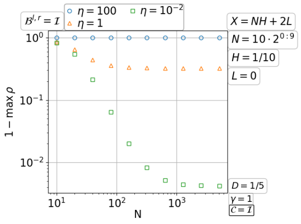
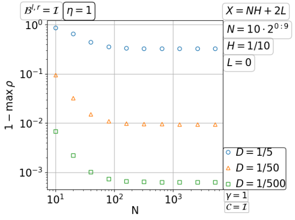
Figure 3.23: Convergence of the double sweep Schwarz method with PML transmission for the Dirichlet problem of diffusion with increasing number of fixed size subdomains.

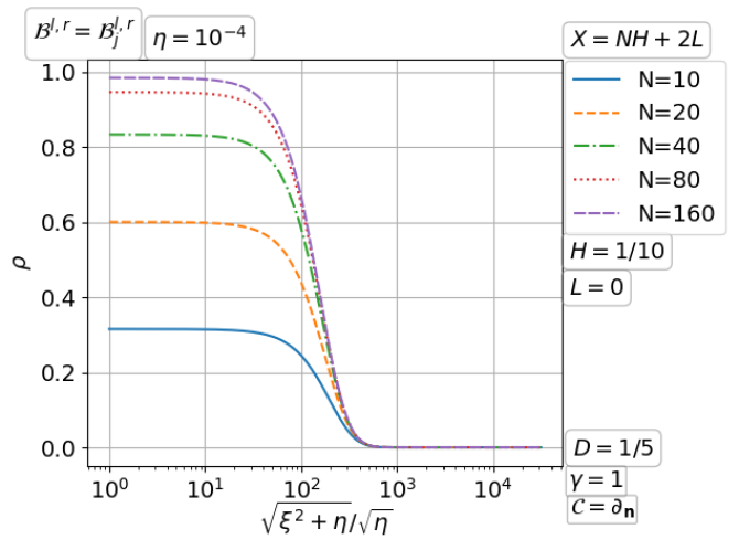
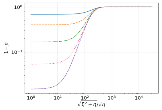
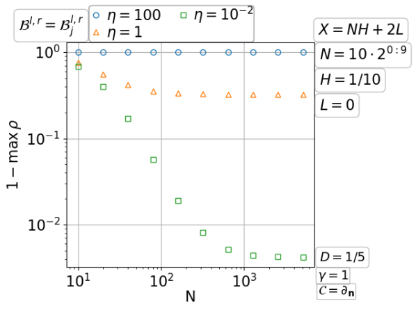
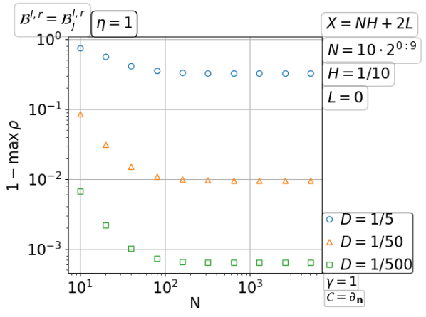
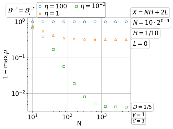
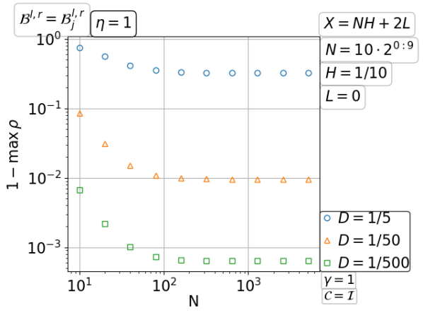
Figure 3.24: Convergence of the double sweep Schwarz method with PML transmission for the infinite pipe diffusion with increasing number of fixed size subdomains.

Convergence on a fixed domain with increasing number of subdomains

In this scaling, we solve a fixed problem with more and more subdomains. Since we are using the PML transmission, the PML width $D$ can be fixed rather than shrinking – an advantage over the overlap. The convergence behavior of the double sweep Schwarz method is illustrated in Figure 3.25, Figure 3.26 and Figure 3.27. Intriguingly, by fixing $D$, the double sweep Schwarz method becomes scalable, which does neither happen to the parallel+PML combination nor to the double sweep+Taylor combination! Not only the maximum of $\rho$ but also the whole graph of $\rho$ is scalable. That is, a limiting profile of $\rho$ seems to exist as $N\to\infty$. Moreover, the terminating condition of PML has a remarkable impact, e.g., when $\eta=10^{-2}$ and $D=1/5$, the difference can be by a factor of about 200. The convergence deterioration with small coefficient $\eta>0$ is mild when the good PML termination is used. Also, it seems that $\max_{\xi}\rho$ decays exponentially to zero as $D$ increases. Hence, given the PML strength $\gamma$, a fixed PML width $D$ is not only sufficient for the scalability but also necessary, for which more evidence can be found in ?.

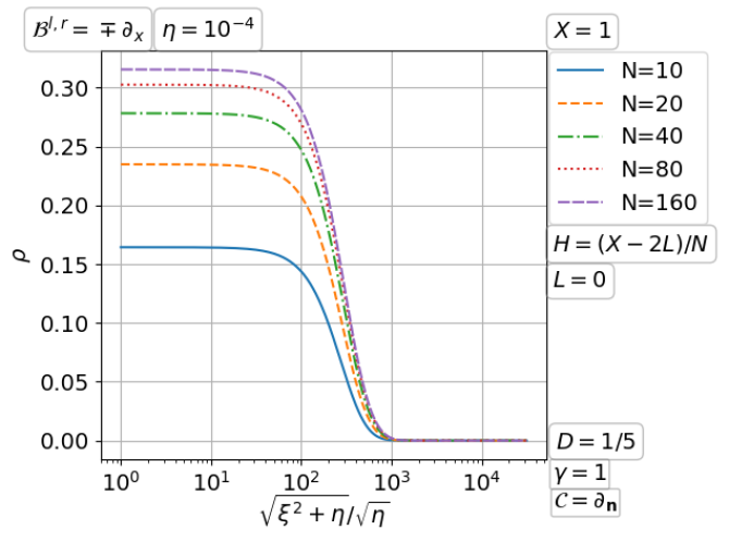
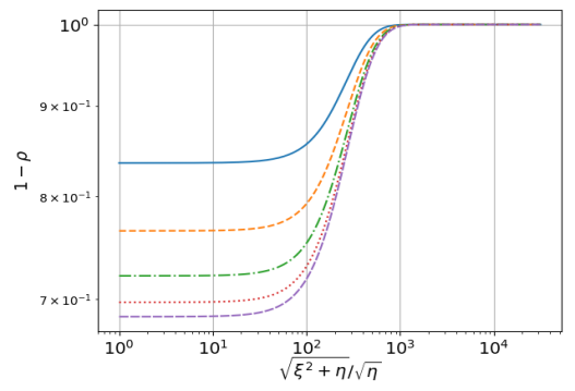
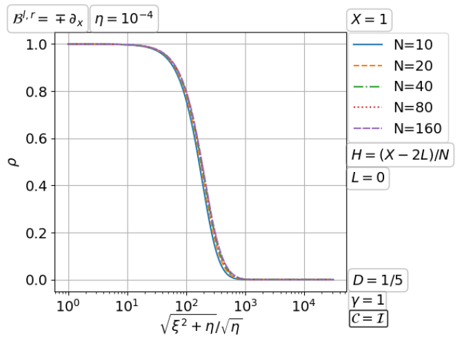
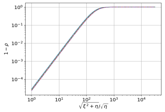
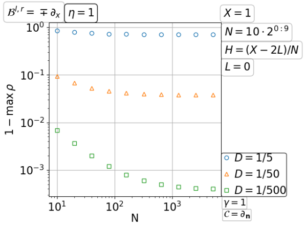
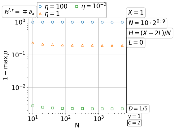
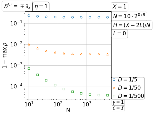
Figure 3.25: Convergence of the double sweep Schwarz method with PML transmission for the Neumann problem of diffusion on a fixed domain with increasing number of subdomains.

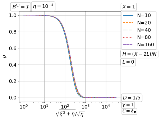
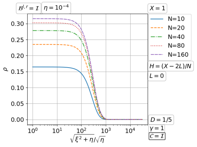
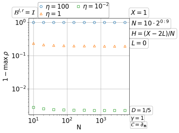
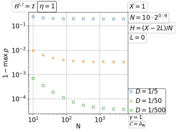
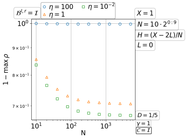
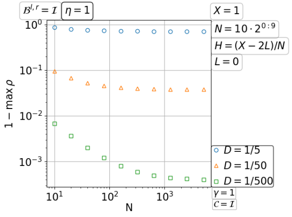
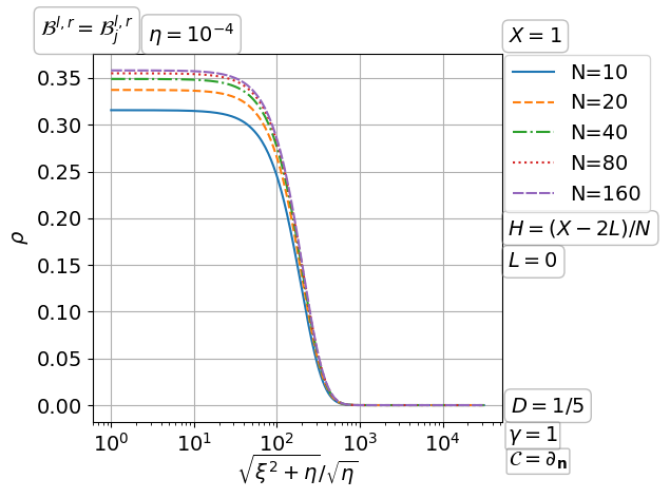
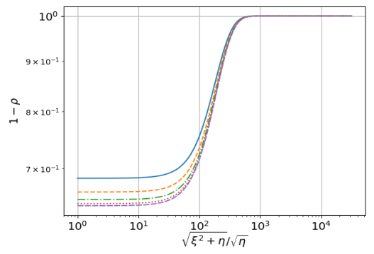
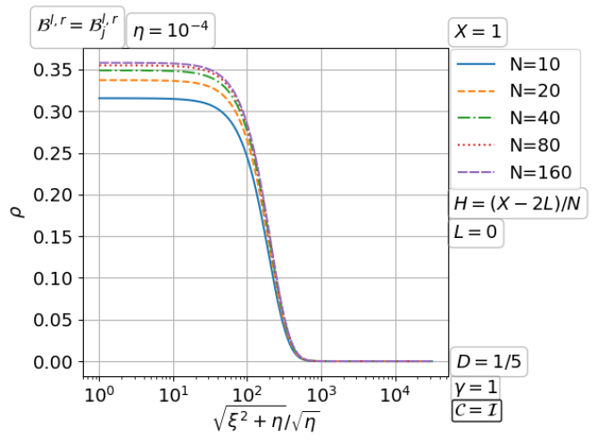
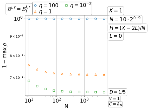
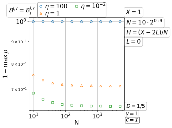
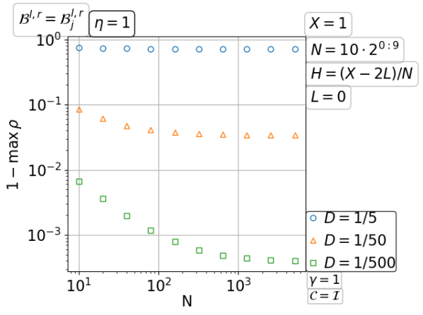
Figure 3.26: Convergence of the double sweep Schwarz method with PML transmission for the Dirichlet problem of diffusion on a fixed domain with increasing number of subdomains.

Figure 3.27: Convergence of the double sweep Schwarz method with PML transmission for the infinite pipe diffusion on a fixed domain with increasing number of subdomains.

3.3 Parallel Schwarz method for the free space wave problem

The free space wave problem corresponds to eqprb with $\mathcal{L}_{x}=-\partial_{xx}$, $\eta=-\omega^{2}$, $\mathcal{B}^{l,r}=\mathcal{B}_{j}^{l,r}$, and $\mathcal{L}_{y}$, $\mathcal{B}^{b,t}$ related to absorbing conditions on bottom and top. If it is the Taylor of order zero condition, then $\mathcal{L}_{y}=-\partial_{yy}$, $\mathcal{B}^{b,t}=\mp\partial_{y}-\I\omega$ and the generalised Fourier frequency $\xi$ from the Sturm-Liouville problem eqsturm is on a curve in the complex plane; see Figure 3.28. For the PML condition on bottom and top, the domain $(0,X)\times(0,1)$ is extended to $(0,X)\times(-D,1+D)$, $\mathcal{L}_{y}=-\tilde{s}\partial_{y}(\tilde{s}\partial_{y})$, $\mathcal{B}^{b,t}=\mp\partial_{y}$ and $\xi=0,\tilde{\xi}\pi,2\tilde{\xi}\pi,3\tilde{\xi}\pi,...$, where $\tilde{s}=1$ on $[0,1]$, $\tilde{s}=(1-\I\tilde{\sigma}(-x))^{-1}$ on $(-D,0)$, $\tilde{s}=(1-\I\tilde{\sigma}(x-1))^{-1}$ on $(1,1+D)$, $\int_{0}^{D}\tilde{\sigma}(x)\D{x}=\frac{1}{2}D\gamma$ and $\tilde{\xi}=((2-\I\gamma)D+1)^{-1}$. The generalised Fourier frequency $\xi$ is on a straight line in the complex plane. For example, when $\gamma=5\pi/\omega$ and $D=1$, the range of $\xi$ is shown in Figure 3.29.

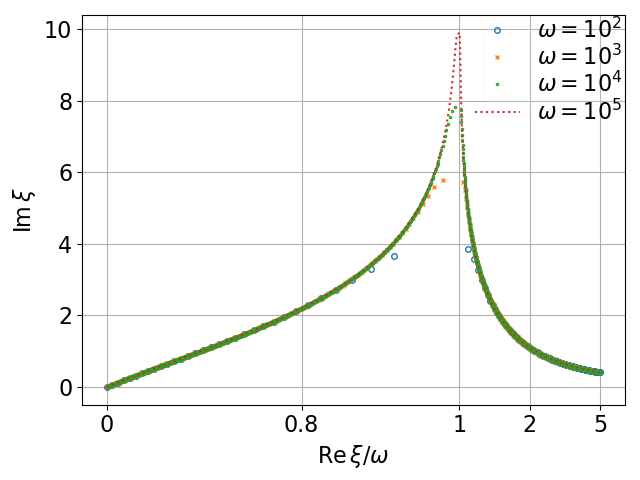
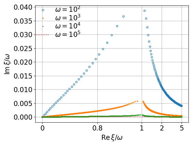
Figure 3.28: Generalised Fourier frequency $\xi$ from the Sturm-Liouville problem eqsturm with $Y=1$, $\mathcal{L}_{y}=-\partial_{yy}$, $\mathcal{B}^{b,t}=\mp\partial_{y}-\I\omega$ (Taylor of order zero condition).

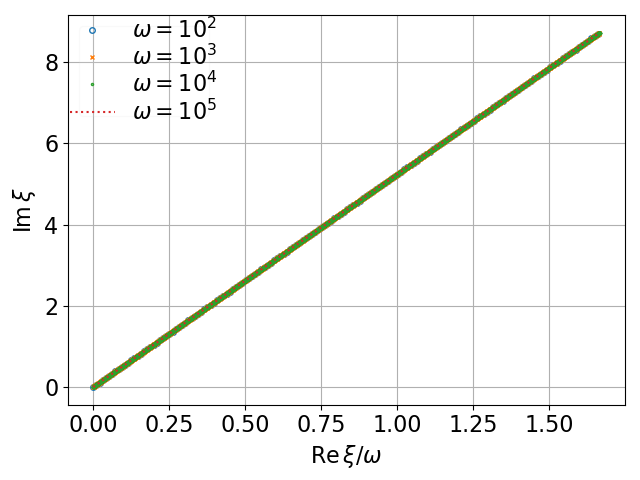
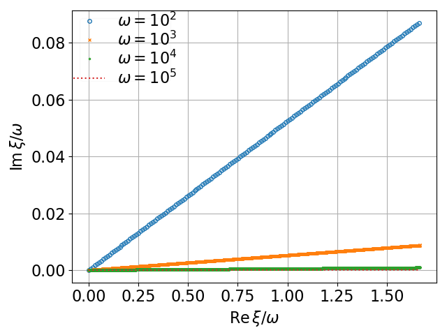
Figure 3.29: Generalised Fourier frequency $\xi$ from the Sturm-Liouville problem eqsturm on the extended domain $(-D,1+D)$ with the PML condition eqpml.

We note that the convergence factor $\rho$ can be viewed as a function of the rescaled Fourier frequency $\xi_{\omega}:=\xi/\omega$, the rescaled subdomain width $H_{\omega}:=\omega H$, the rescaled overlap width $L_{\omega}:=\omega L$ and the number of subdomains $N$. But the range of the generalised Fourier frequency $\xi$ depends on the wavenumber $\omega$ through the original boundary condition on top and bottom. Increasing $\omega$ is not only to have more sampling points $\frac{\Re\xi}{\omega}\in\mathbb{R}$ but also to decrease $\frac{\Im\xi}{\omega}$; see again Figure 3.28 and Figure 3.29. So, the dependence of $\rho$ on $\omega$ is of particular interest besides the dependence on $\xi$, $H$, $L$ and $N$.

There are not many theoretical results on the convergence of Schwarz methods for the Helmholtz equation. ? in his thesis proposed the first Schwarz method for the Helmholtz equation. He replaced the classical overlapping Dirichlet transmission with the non-overlapping Taylor of order zero transmission, and he proved the convergence of the resulting Schwarz iteration in general geometry, arbitrary decomposition and variable media as long as part of the original boundary is equipped with the Taylor of order zero condition. That idea has been further developed and generalised. ? showed that for a decomposition without cross points the convergence of the relaxed Schwarz iteration can be geometric if the Taylor of order zero transmission $\partial_{\mathbf{n}}+\I\omega$ is enhanced by a square-root operator to $\partial_{\mathbf{n}}+\I\omega\sqrt{\alpha-\beta\omega^{-2}\partial_{yy}}$. ? analyzed the discrete version and showed that the convergence rate is uniform in the mesh size. For recent progress along the direction of nonlocal transmission conditions, see ?, ?, ?, ?, ?. For local transmission conditions, the convergence rate of the Schwarz preconditioned Krylov iteration was first analyzed by ? and then generalised by ?, ?. Besides the above general theories, convergence for domain decomposition in a rectangle has also been studied. ? considered the high wavenumber asymptotic. A variational interpretation of the Schwarz preconditioner was discussed in ?, and an analysis at the discrete level was given in ?. ? gave the first convergence estimate of the double sweep Schwarz method with PML transmission. A recursive double sweep Schwarz method was analyzed by ?. For the waveguide problem, we refer to ?, ?, ?.

3.3.1 Parallel Schwarz method with Taylor of order zero transmission for the free space wave problem

In this case, we assume that the original boundary condition is also the Taylor of order zero condition, i.e., $\mathcal{B}^{b,t}=\mathcal{B}^{l,r}=\mathcal{B}^{l,r}_{j}$. According to ?, the parallel Schwarz method with non-overlapping Taylor of order zero transmission converges. However, the convergence rate for the evanescent modes is very slow. To mitigate the situation, here we shall add an overlap, though the convergence is no longer guaranteed by any theory. On the one hand, divergence was observed if the overlap exceeds a threshold related to the wavenumber $\omega$ and the subdomain width $H$. On the other hand, intuitively, we still expect convergence if the overlap is sufficiently small, which we will find to be the case from the following paragraphs, see also the two subdomain case in Section 2. Indeed, we carried out a scaling test of shrinking overlap $L\to 0$ on a fixed domain with 10 subdomains and fixed wavenumber and found the same scaling as in TaylorRhoRRHelmholtz.

Convergence with increasing number of fixed size subdomains

The graph of the convergence factor $\rho=\rho(\xi)$ is shown in the top half of Figure 3.30. Note that, for a finite number of subdomains $N$, $\rho(0)=0$ because the Taylor expansion in the transmission condition is exactly at the point $\xi=0$, but $\rho$ grows drastically in the neighborhood of $\xi=0$. Actually we see that $\rho_{\infty}:=\lim_{N\to\infty}\rho$ is tending to one as $\xi\to 0$. Note also that there is no singularity at $\Re\xi=\omega$ because $\Im\xi\neq 0$ due to the top and bottom Taylor of order zero conditions (see Figure 3.28), and the convergence of the evanescent modes corresponding to $\Re\xi>\omega$ is good and independent of $N$. Given the limiting graph $\rho_{\infty}$, we see that as $N\to\infty$, the maximum point of $\rho$ decreases toward zero. Since $\xi$ is discrete and $\rho(0)=0$, it seems that for sufficiently large $N$ the maximum of $\rho$ will be attained at the first nonzero Fourier frequency $\xi_{1}$ (close to $\pi$) and the maximum value tends to $\rho_{\infty}(\xi_{1})$. But this asymptotic is hardly observed up to $N=5200$ in the bottom half of Figure 3.30. Rather, we find $\max_{\xi}\rho=1-O(N^{-1})$ in most cases. An exception occurs in the bottom left subplot when $\omega=100$, $H=1/20$ and $L=H/40$, for which $\max_{\xi}\rho=1-O(N^{-3/2})$ is observed.

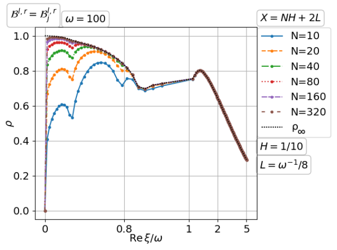
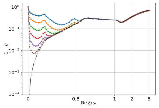
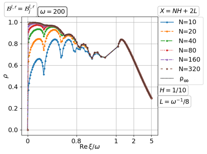
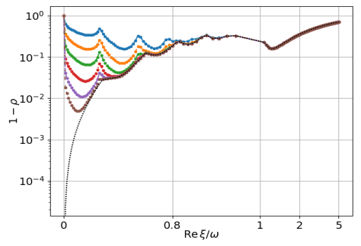
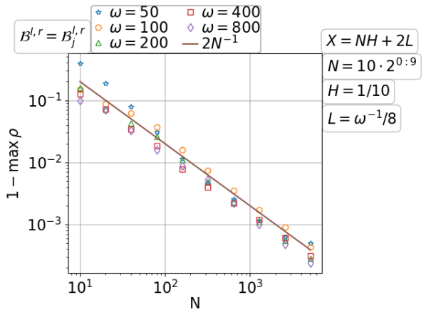
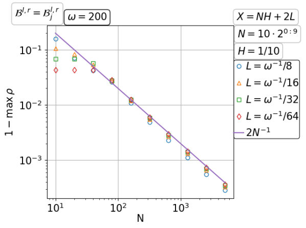
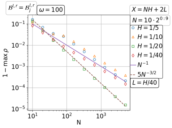
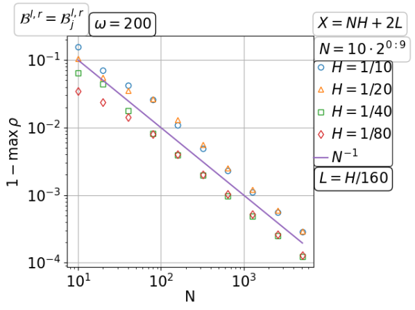
Figure 3.30: Convergence of the parallel Schwarz method with Taylor of order zero transmission for the free space wave with increasing number of fixed size subdomains.

Convergence on a fixed domain with increasing number of subdomains

Now we increase the number of subdomains $N$ for a fixed domain width $X$ and a fixed wavenumber $\omega$. This time all the modes have slower convergence for bigger $N$; see the top half of Figure 3.31. Away from $\xi=0$, the behavior of $\rho$ can be explained by that of the limiting curve $\rho_{\infty}$ with the corresponding subdomain width $H=(X-2L)/N\to 0$. As $N$ grows, the maximum point of $\rho$ can change between the two regions $\Re\xi/\omega<1$ and $\Re\xi/\omega>1$. This is because smaller $L$ benefits convergence of the propagating modes but hinders convergence of the evanescent modes. Nevertheless, a scaling of $\max_{\xi}\rho$ with $N\to\infty$ still appears; see the bottom half of Figure 3.31. It is estimated that $\max_{\xi}\rho=1-O(N^{-5/3})$ if $L=O(H)$ is sufficiently small and $\max_{\xi}\rho=1-O(N^{-5/2})$ if $L=O(H^{2})$ is sufficiently small.

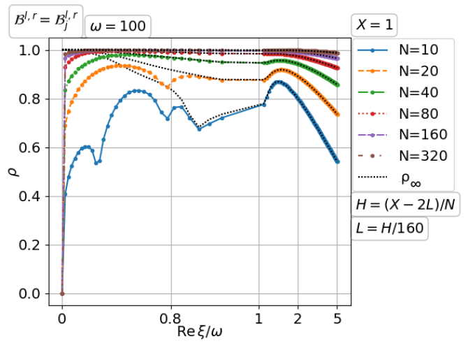
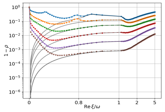
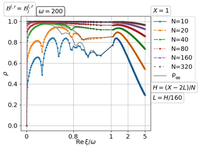
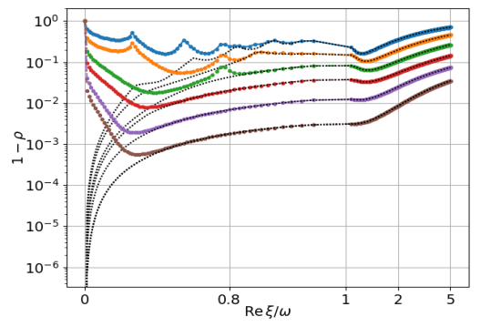
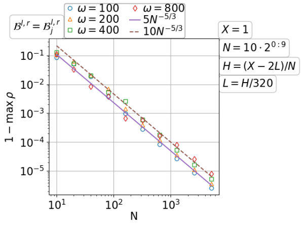
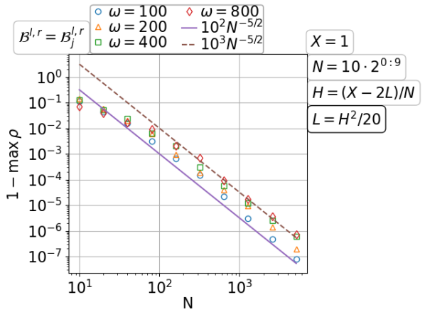
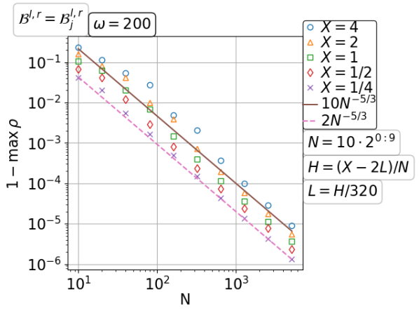
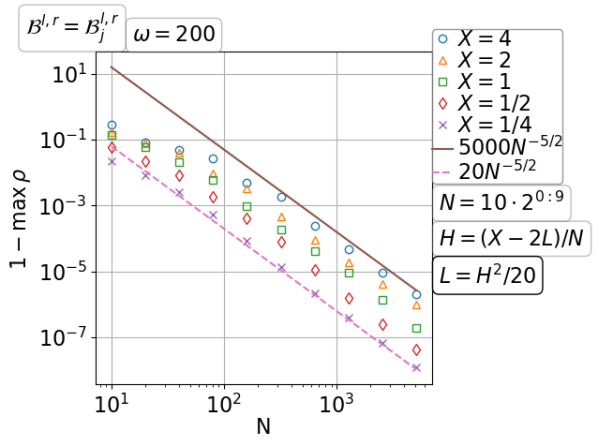
Figure 3.31: Convergence of the parallel Schwarz method with Taylor of order zero transmission for the free space wave on a fixed domain with increasing number of subdomains.

Convergence on a fixed domain with a fixed number of subdomains for increasing wavenumber

We show the graph of the convergence factor $\rho$ for the domain width $X=1$, the number of subdomains $N=40$, the overlap width $L=\omega^{-1}/40$ and growing wavenumber $\omega$ in the top half of Figure 3.32. We find that the graph of $1-\rho$ has a limiting profile in the propagating region $\Re\xi/\omega<1$ as $\omega\to\infty$ and has a unique local minimum in the evanescent region $\Re\xi/\omega>1$ which decreases as $\omega\to\infty$. So, the Schwarz method is preasymptotically robust about $\omega$ until the local maximum of $\rho$ over $\Re\xi/\omega>1$ becomes dominating –a phenomenon observed numerically in ?. The asymptotic scaling is estimated in the bottom half of Figure 3.32 as $\max_{\xi}\rho=\max_{\Re\xi>\omega}\rho=1-O(\omega^{-9/20})$ for $L=O(\omega^{-1})$ and $1-O(\omega^{-2/3})$ for $L=O(\omega^{-3/2})$.

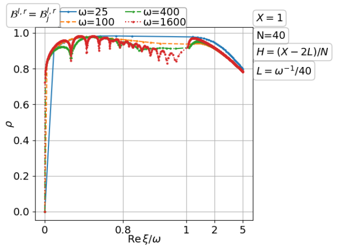
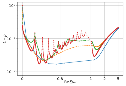
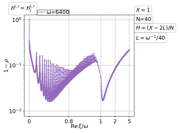
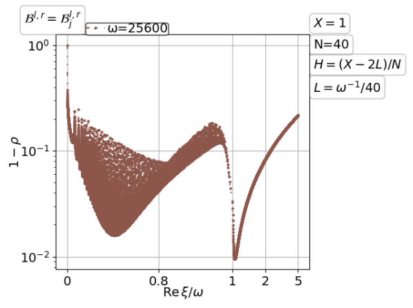
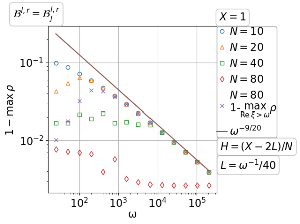
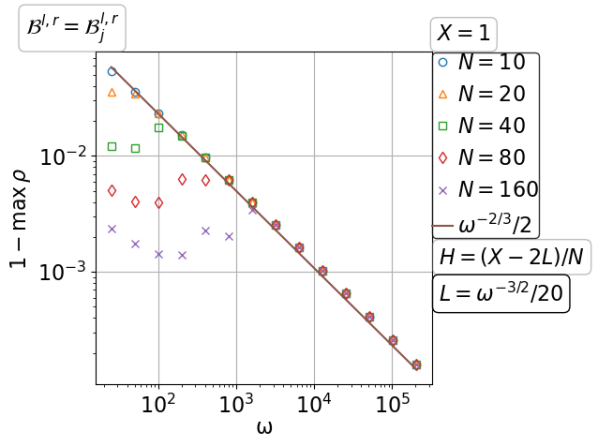
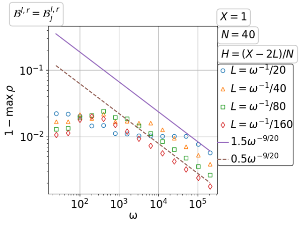
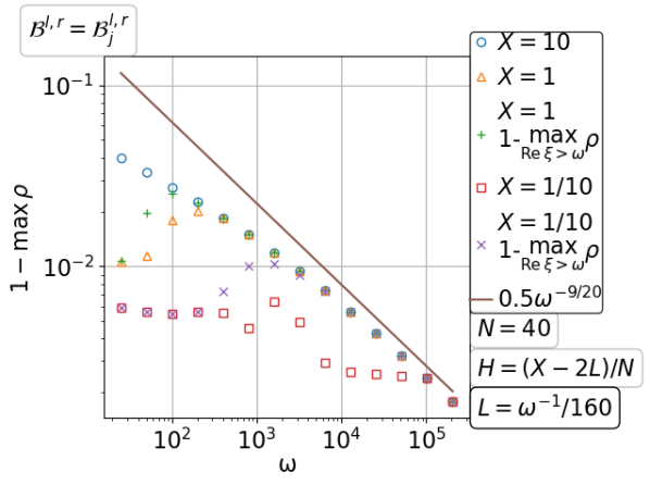
Figure 3.32: Convergence of the parallel Schwarz method with Taylor of order zero transmission for the free space wave on a fixed domain with a fixed number of subdomains for increasing wavenumber.

Convergence on a fixed domain with number of subdomains increasing with the wavenumber

The scaling here is more challenging because both the increasing wavenumber and the shrinking subdomain width force the overlap width $L$ to be small, and $L=O(\omega^{-1})$ is not small enough for convergence. We use $L=O(\omega^{-3/2})$ in the top half of Figure 3.33 for the graph of the convergence factor $\rho=\rho(\xi)$. Both the local maxima of $\rho$ in the two regions $\Re\xi<\omega$ and $\Re\xi>\omega$ increase with $N$, with the first one increasing faster and the seccond one dominating in the preasymptotic regime. The scaling of $\max_{\xi}\rho$ is estimated in the bottom half of Figure 3.33. Asymptotically $\max_{\xi}\rho=1-O(N^{-2})$ for $L=O(\omega^{-3/2})$ and $\max_{\xi}\rho=1-O(N^{-5/3})$ for $L=O(\omega^{-2})$, while the preasymptotic scaling is better.

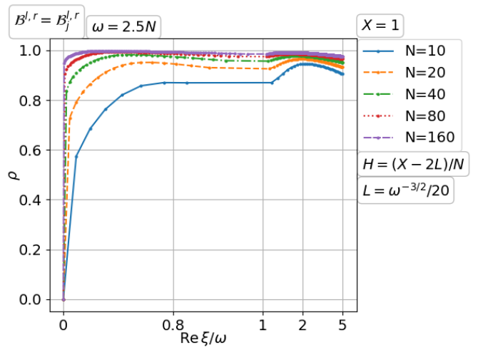
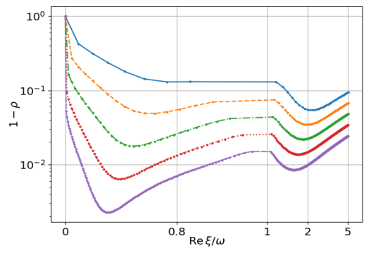
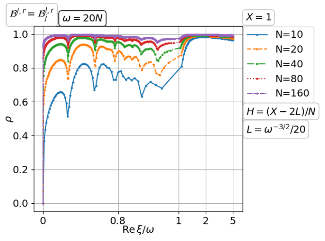
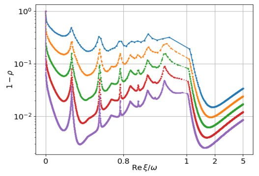
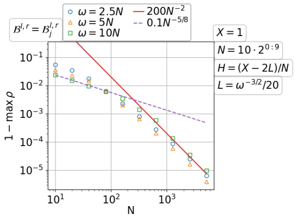
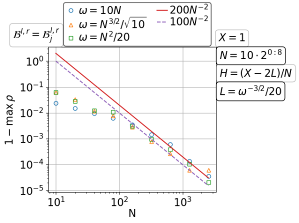
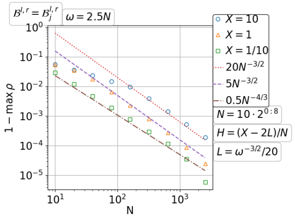
Figure 3.33: Convergence of the parallel Schwarz method with Taylor of order zero transmission for the free space wave on a fixed domain with number of subdomains increasing with the wavenumber.

3.3.2 Parallel Schwarz method with PML transmission for the free space wave problem

In this case, we assume that the original boundary condition is also the PML condition, i.e., $\mathcal{B}^{b,t}=\mathcal{B}^{l,r}=\mathcal{B}_{j}^{l,r}$. For analysis purposes, the PML on the left and right is regarded as a boundary condition involving eqsw, while the PML on top and bottom is treated as part of the extended domain. The use of PML transmission conditions for parallel Schwarz methods can be traced back to ?, see also ?, ?, ?. It is combined with a coarse space in ?. Since the PML condition can be made arbitrarily close to the exact transparent condition, i.e., the PML Dirichlet-to-Neumann operator eqsw can approximate the exact Dirichlet-to-Neumann operator to arbitrary accuracy, we can expect the Schwarz method to converge as soon as the PML is sufficiently accurate; see also ?. This has been first quantified by ?, though for the double sweep Schwarz method. There is a pending issue about how accurate the PML needs to be to ensure a robust convergence. We shall address the issue at the continuous level for the parallel Schwarz method under different scalings in this subsection.

Convergence with increasing number of fixed size subdomains

On the first row of Figure 3.34, we check the influence of the terminating condition of the PML. One effect is from the top and bottom PMLs. The Neumann terminated PMLs give the zero frequency $\xi=0$, while the Dirichlet terminated PMLs do not. This has already made a difference on the convergence. The limiting convergence factor $\rho_{\infty}$ for the Neumann terminated PMLs is actually greater than one at $\xi=0$, while that for the Dirichlet terminated PMLs is less than one over the range of frequencies. Otherwise, quantitively the terminating condition of the PMLs makes little difference. The graph of the convergence factor $\rho$ in the top half of Figure 3.34 looks somewhat similar to Figure 3.14 for the diffusion problem: both are better at higher frequencies $\xi$. Roughly speaking, the PML works like an overlap but with all the modes decaying inside it, and the top and bottom PMLs make the decaying faster for higher frequencies. As we have encountered for the diffusion problem, the parallel Schwarz method with a fixed PML for the wave problem also slows down with increasing number of subdomains $N$. A logarithmic growth of the PML width $D$ with $N$ does not change the scaling; see the third row of Figure 3.34, where the dependence on the wavenumber $\omega$ is also measured. Then, in the last row of the figure, we recorded the dependence on $D$ and the subdomain width $H$. We actually find that $1-\max_{\xi}\rho=O(N^{-1})$ improves its hidden factor as $D$ grows and is essentially independent of $H$ and $\omega$.

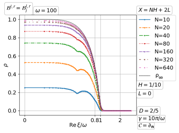
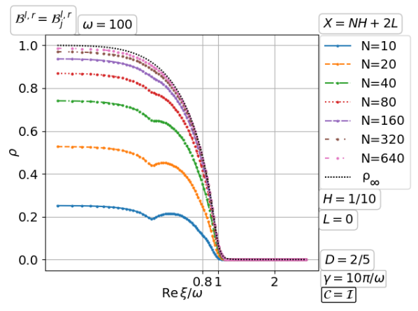
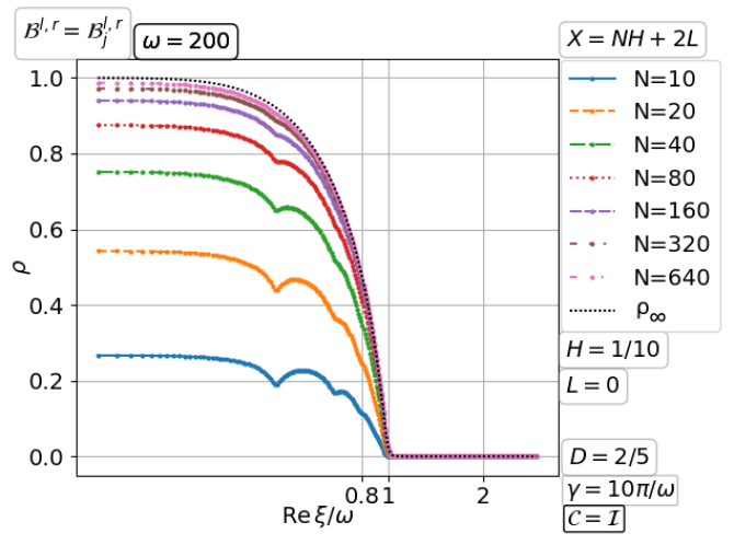
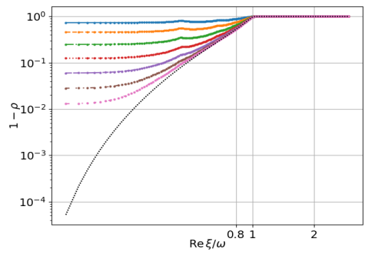
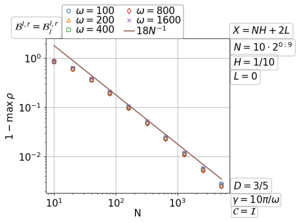
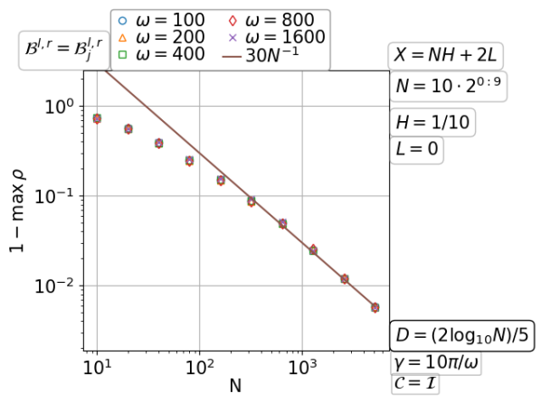
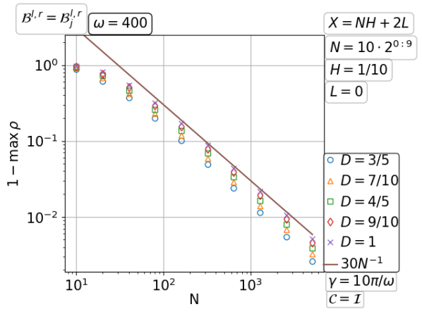
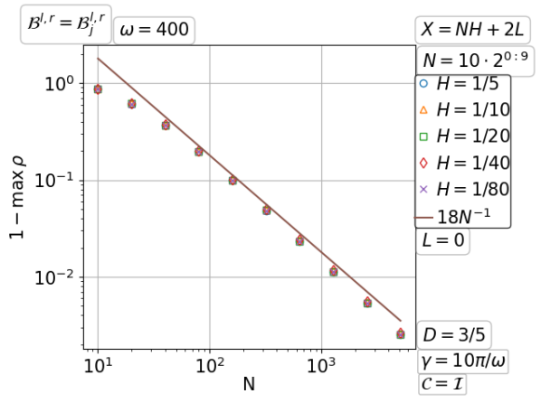
Figure 3.34: Convergence of the parallel Schwarz method with PML transmission for the free space wave with increasing number of fixed size subdomains.

Convergence on a fixed domain with increasing number of subdomains

Now we consider solving a fixed problem with increasing number of subdomains $N$. In the top half of Figure 3.35, the graph of the convergence factor $\rho=\rho(\xi)$ for each $N$ is plotted along with the limiting convergence factor $\rho_{\infty}$ with the corresponding $H=X/N$. In this case, $\rho$ is much better than $\rho_{\infty}$, similar to that for the diffusion problem (see Figure 3.17). The scaling of $\max_{\xi}\rho$ and its dependence on the wavenumber $\omega$ are measured on the third row of Figure 3.35. On the right, the PML width $D$ grows logarithmically with $N$, and we see that when $D$ becomes sufficiently large, $\max_{\xi}\rho$ drops to numerical zero. However, this does not mean that the convergence does not depend on the number of subdomains $N$, because the optimal parallel Schwarz iteration is nilpotent of index $N$. The last row of the figure checks the dependence on $D$ and the domain width $X$. We find $\max_{\xi}\rho=1-O(N^{-1})$ which improves its hidden factor as $D$ grows and depends very mildly on $X$.

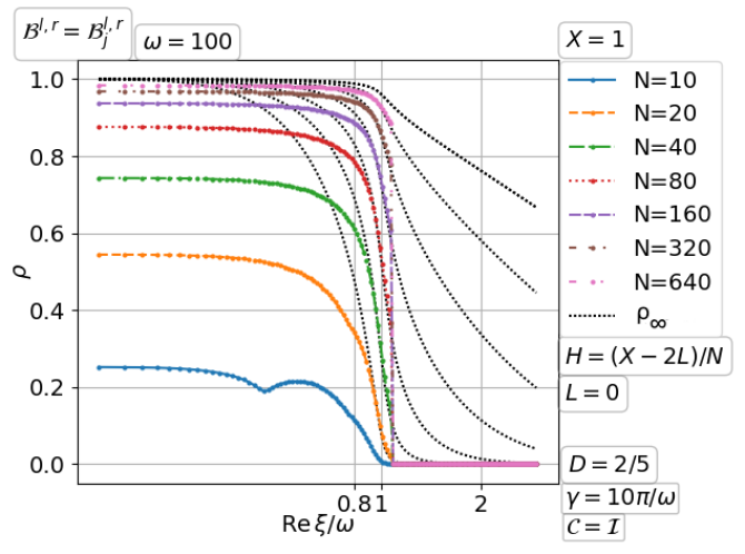
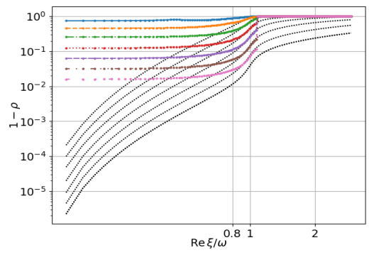
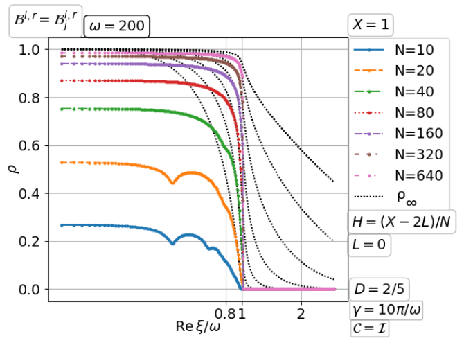
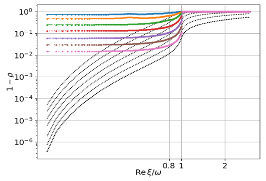
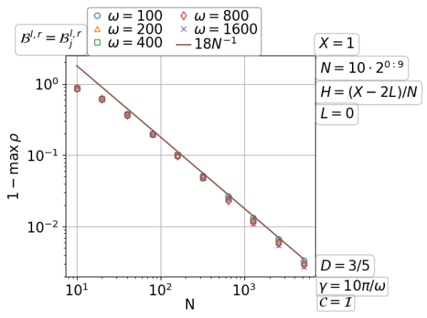
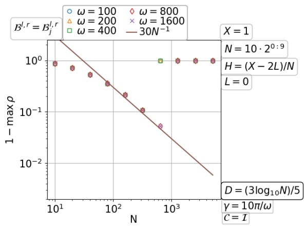
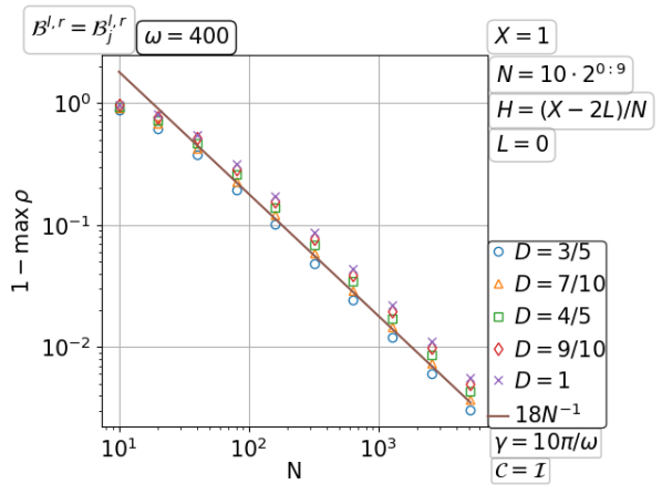
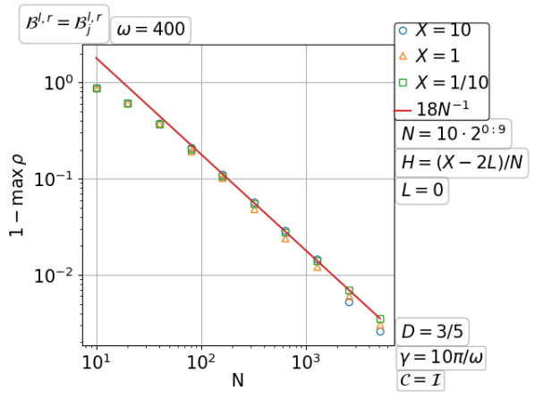
Figure 3.35: Convergence of the parallel Schwarz method with PML transmission for the free space wave on a fixed domain with increasing number of subdomains.

Convergence on a fixed domain with a fixed number of subdomains for increasing wavenumber

The scaling with the wavenumber $\omega$ is studied while all the other parameters are fixed. A limiting profile of the convergence factor $\rho$ as $\omega\to\infty$ is indicated in the top half of Figure 3.36. The scaling of $\max_{\xi}\rho$ with $\omega$ and its dependence on the number of subdomains $N$, the PML width $D$ and the domain width $X$ are explored one by one in the bottom half of the figure. We find $\max_{\xi}\rho=O(1)<1$ which increases with $N$ (superlinearly at high wavenumber $\omega$), decays exponentially with $D$ and depends mildly on $X$.

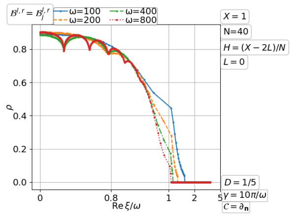
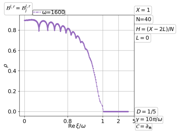
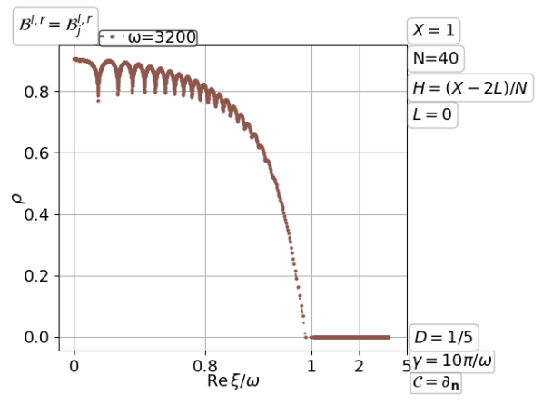
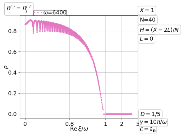
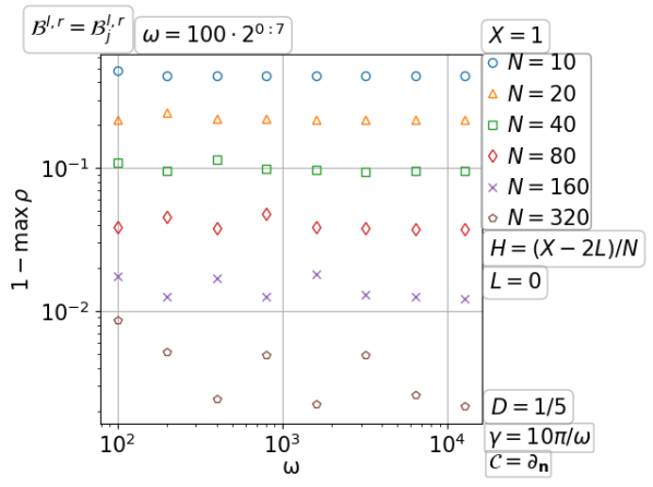
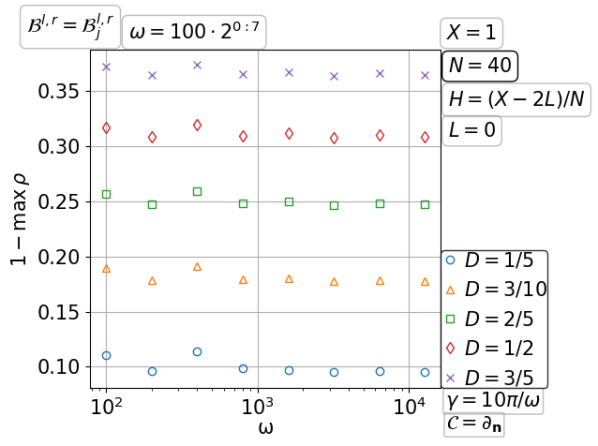
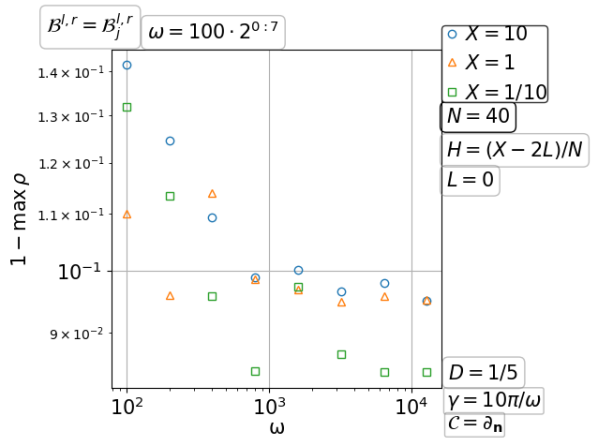
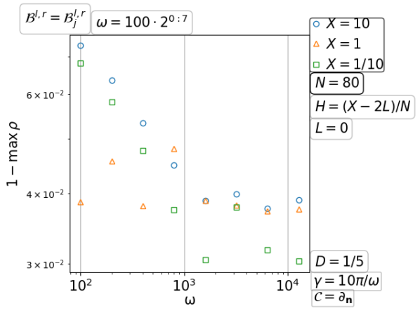
Figure 3.36: Convergence of the parallel Schwarz method with PML transmission for the free space wave on a fixed domain with a fixed number of subdomains for increasing wavenumber.

Convergence on a fixed domain with number of subdomains increasing with the wavenumber

In the previous scalings, we have found that the subdomain width $H$ and the wavenumber $\omega$ have little influence on the convergence of the parallel Schwarz method with a fixed PML transmission, and the convergence slows down mainly due to an increasing number of subdomains $N$. While larger PML width $D$ accelerates the convergence and can even make the convergence factor $\rho$ numerical zero, the dependence on $N$ is inherent from the nilpotency index of the optimal parallel Schwarz iteration matrix which has the symbol entries $a_{j}=c_{j}=\exp(-\I\sqrt{\omega^{2}-\xi^{2}}H)$ of modulus about $1$ for the propagating modes ($\Re\xi<\omega$). Now in Figure 3.37, we increase also the wavenumber $\omega$ with $N$. It can be seen that the scaling $\max_{\xi}\rho=1-O(N^{-1})$ is the same as for fixed $\omega$ in Figure 3.35.

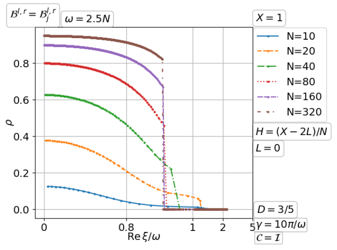
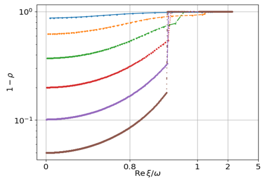
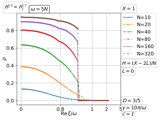
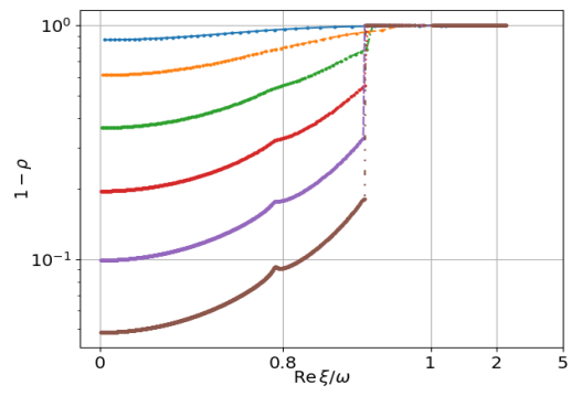
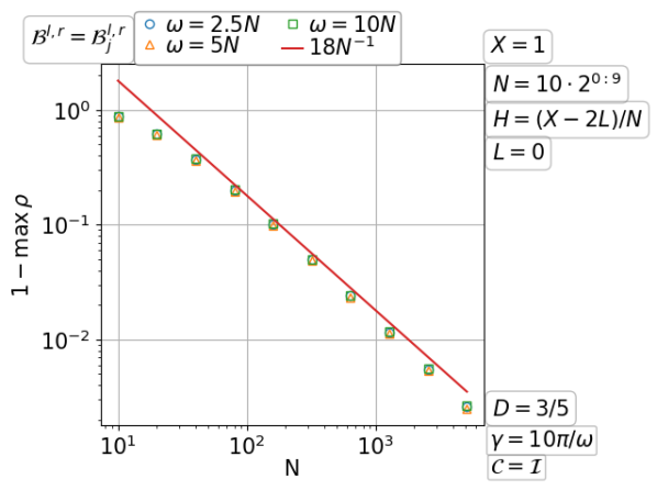
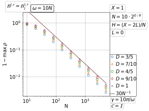
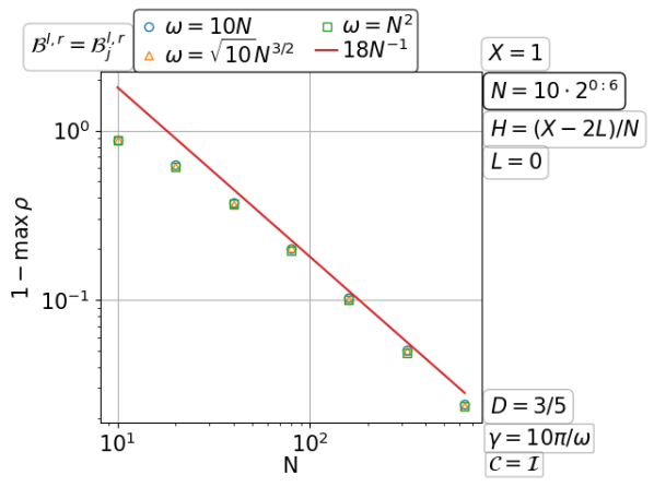
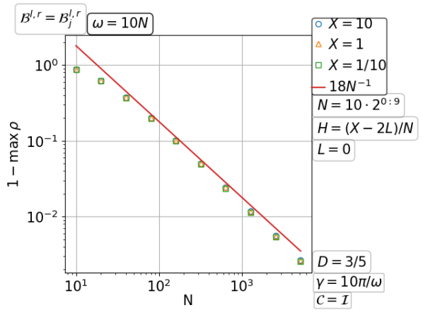
Figure 3.37: Convergence of the parallel Schwarz method with PML transmission for the free space wave on a fixed domain with number of subdomains increasing with the wavenumber.

3.4 Double sweep Schwarz method for the free space wave problem

We have already seen for the parallel Schwarz methods that the free space wave problem is significantly more difficult than the diffusion problem. For example, with fixed size subdomains, the free space wave problem requires the parallel Schwarz iteration number to grow linearly with number of subdomains $N$ even with the wavenumber $\omega$ fixed, while the diffusion problem requires only a constant iteration number. The Taylor of order zero transmission and the PML transmission lead to the same scalings for the diffusion problem, while for the wave problem a sufficient PML is necessary to guarantee convergence of the parallel Schwarz method and leads to much faster convergence than the Taylor of order zero transmission conditions do. We also note that the parallel Schwarz method with a fixed PML on a fixed domain has the same scalings of the convergence rate for the wave and the diffusion problems.

Another angle of view is to compare the parallel Schwarz methods with their double sweep counterparts, which has been presented for the diffusion problem. We have seen that the dependence of the convergence rate on the number of subdomains can be removed by using together a fixed PML transmission and the double sweep Schwarz iteration.

Now we are going to study the double sweep Schwarz methods for the free space wave problem. Do they scale with fixed size subdomains, given that the parallel Schwarz methods do for the diffusion problem but not for the wave problem? With Taylor of order zero transmission without overlap, the parallel Schwarz method is proved to converge (?). Do we still expect convergence when we change only the parallel iteration to the double sweep iteration? How do the double sweep Schwarz methods depend on the wavenumber? Will a fixed PML make the convergence scalable with the number of subdomains like it does for the diffusion problem?

3.4.1 Double sweep Schwarz method with Taylor of order zero transmission for the free space wave problem

For the free space problem, we assume that the original boundary condition is also the Taylor of order zero condition, i.e., $\mathcal{B}^{b,t}=\mathcal{B}^{l,r}=\mathcal{B}^{l,r}_{j}$. There is no theoretical convergence result for the double sweep Schwarz method with Taylor of order zero transmission. Our experience with the parallel Schwarz method is that a sufficiently small overlap allows convergence of both evanescent and propagating modes. We shall try different overlap width $L$ in the following study.

Convergence with increasing number of fixed size subdomains

When the domain grows by adding fixed size subdomains along one direction and the wavenumber $\omega$ is fixed, we find a suitable overlap width can be $L=O(\omega^{-1})$; see the top half of Figure 3.38. Although not shown in the figure, now not only too large overlap can cause divergence of some propgating modes but also too small overlap can cause divergence of some evanescent modes! From the figure, we can see that a limiting curve $\rho_{\infty}:=\lim_{N\to\infty}\rho$ exists for the double sweep Schwarz method, and $\rho$ grows with $N$ towards $\rho_{\infty}$. The tendency indicates quite good convergence at large $N$, which is verified in the bottom half of the figure. We find $\max_{\xi}\rho=O(1)<1$ which deteriorates with increasing wavenumber $\omega$, shrinking overlap width $L$ and shrinking subdomain width $H$.

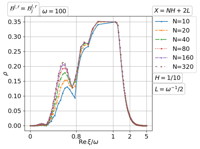
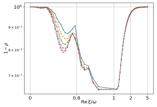
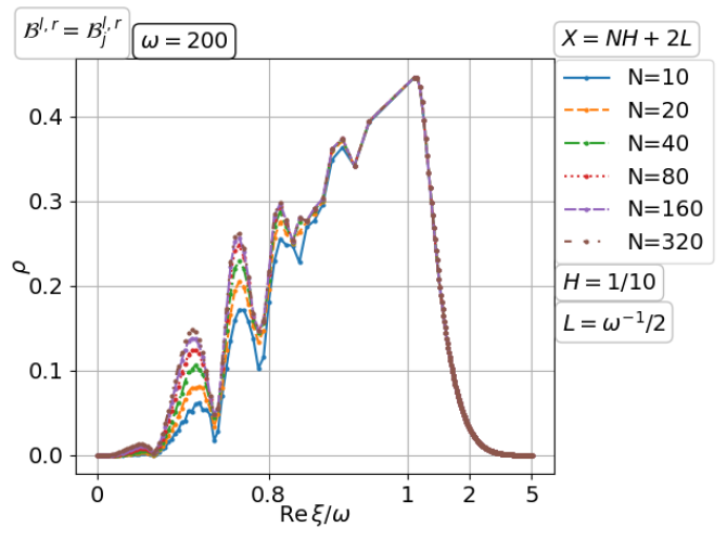
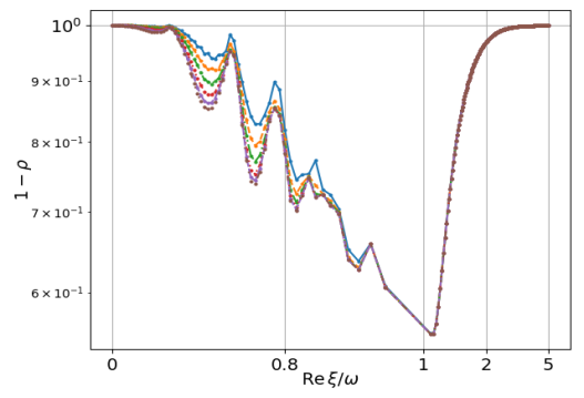
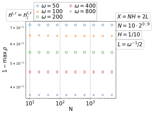
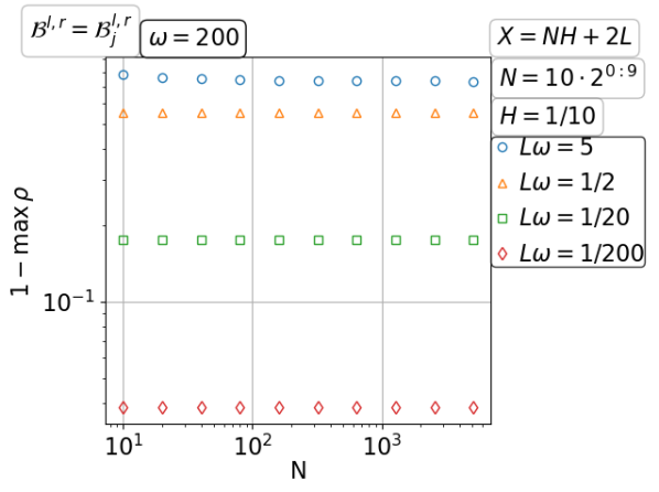
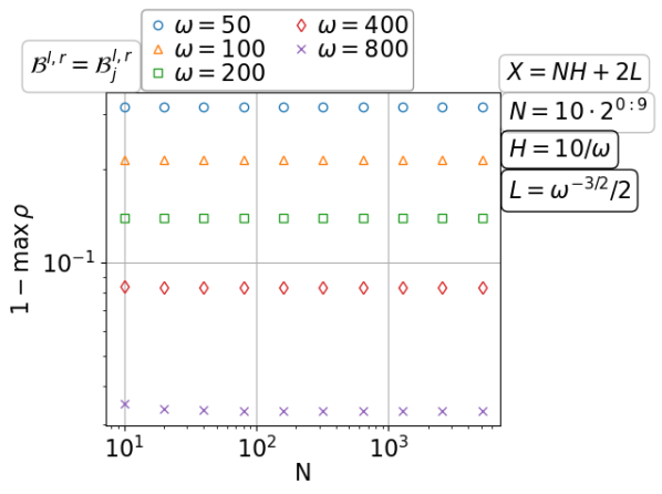
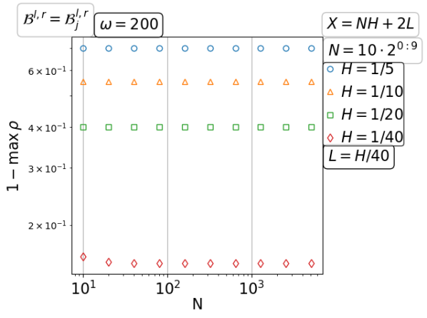
Figure 3.38: Convergence of the double sweep Schwarz method with Taylor of order zero transmission for the free space wave with increasing number of fixed size subdomains.

Divergence on a fixed domain with increasing number of subdomains

As we mentioned before, the overlap width $L$ should be small for convergence of propagating modes and also should be large for convergence of evanescent modes. The two opposite requirements become difficult to satisfy when the subdomain width $H$ is small. Figure 3.39 illustrates this: we see that the double sweep Schwarz method can not converge for these examples with whatever overlap. In other words, under the scaling with increasing number of subdomains on a fixed domain, the double sweep Schwarz method with Taylor of order zero transmission eventually diverges.

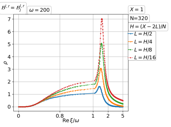
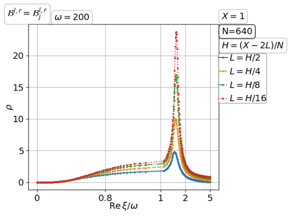
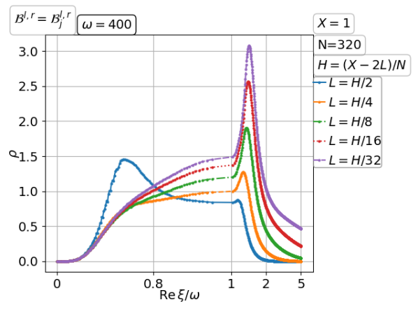
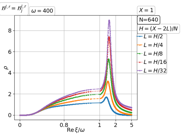
Figure 3.39: Divergence of the double sweep Schwarz method with Taylor of order zero transmission for the free space wave on a fixed domain with increasing number of subdomains.

Convergence on a fixed domain with a fixed number of subdomains for increasing wavenumber

As we learned from the previous paragraphs, when the subdomain width is sufficiently large, the double sweep Schwarz method with Taylor of order zero transmission converges with a suitable overlap width. In the convergent regime, we can still study the scaling with the wavenumber $\omega$; see Figure 3.40. The top half illustrates the changing graph of $\rho=\rho(\xi)$ with $\omega$, which shows a limiting profile away from a neighborhood of $\Re\xi=\omega$, and its maximum attained near $\Re\xi=\omega$ increases with $\omega$. The bottom half of the figure shows the estimate $\max_{\xi}\rho=1-O(\omega^{-9/20})$ for large $\omega$, with the hidden factor independent of number of subdomains $N$ and the domain width $X$.

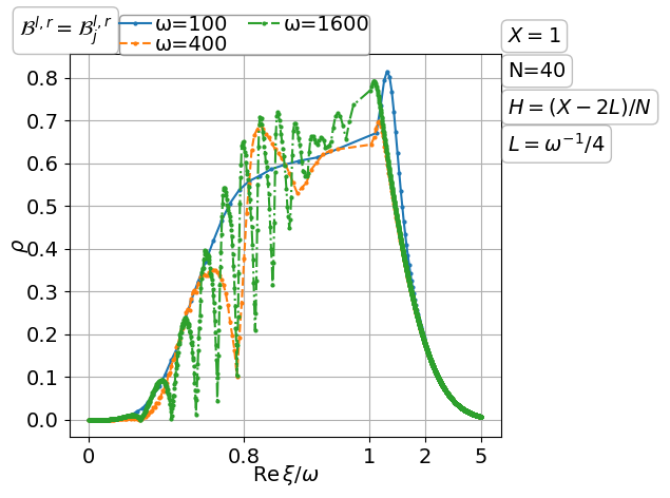
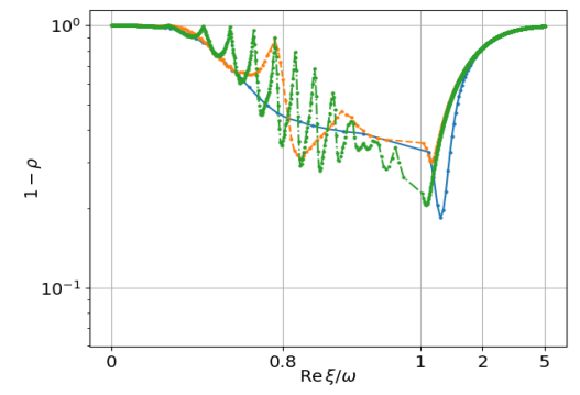
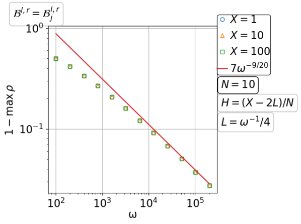
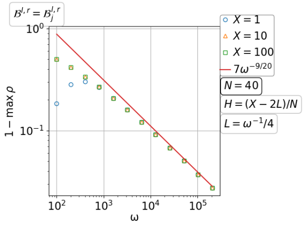
Figure 3.40: Convergence of the double sweep Schwarz method with Taylor of order zero transmission for the free space wave on a fixed domain with a fixed number of subdomains for increasing wavenumber.

Divergence on a fixed domain with number of subdomains increasing with the wavenumber

As we mentioned before, convergence of the double sweep Schwarz method with Taylor of order zero transmission requires a sufficienly large subdomain width $H$. So, on a fixed domain under the scaling $N\to\infty$, the method eventually must diverge. That the wavenumber increases here with $N$ does not change the situation. As can be seen in Figure 3.41, divergence of some propagating modes is persistent at large $N$ for any overlap width $L$ including $L=0$.

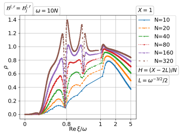
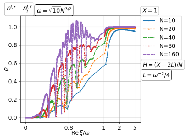
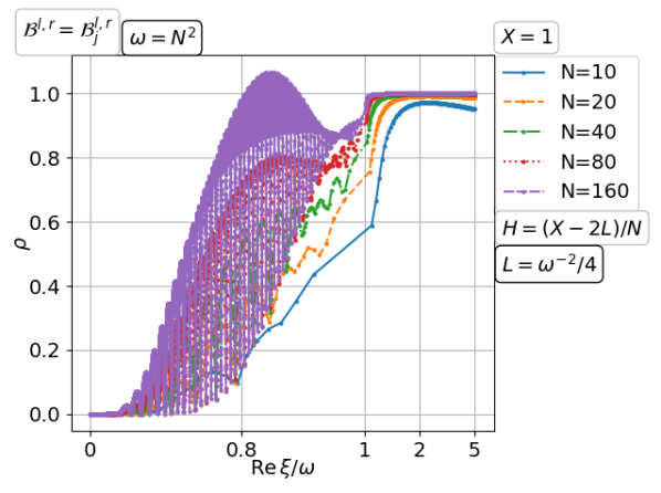
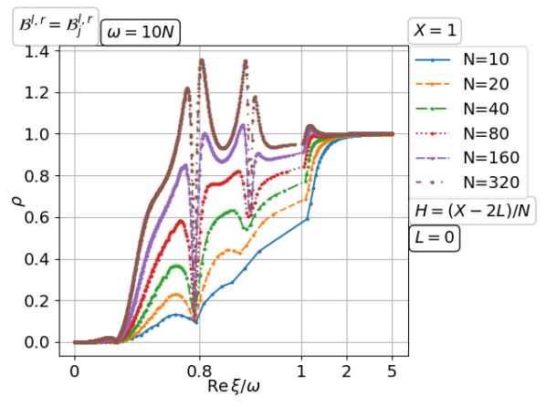
Figure 3.41: Divergence of the double sweep Schwarz method with Taylor of order zero transmission for the free space wave on a fixed domain with number of subdomains increasing with the wavenumber.

3.4.2 Double sweep Schwarz method with PML transmission for the free space wave problem

For the free space problem, the PML is used all around the domain. The top and bottom PML is treated as part of the extended domain. For analysis purposes, the left and right PML for the subdomains and the domain goes into the Dirichlet-to-Neumann operator eqsw in the boundary condition listed in Table 5. The double sweep Schwarz method with PML transmission for the free space wave problem is the most noticeable case in the last decade. Impressive numerical experiments have been shown in the literature; see e.g. ?, ?, ?, ?, ?, ?, ?, ?, ?. Recently, it was applied to an inverse problem (?). An interesting attempt is to use double sweeps in small groups of connected subdomains for accelerating the corresponding parallel Schwarz method (?). A question that has not been answered in theory is how many discrete layers of PML are needed for scalable iterations. ? have an estimate at the continuous level indicating that a PML width $D=O(N\log\omega)$ is sufficient. It was claimed based on numerical experiments that a logarithmic growth of discrete layers of PML could be sufficient for increasing wavenumber $\omega$ but fixed oscillations $\omega H$ in the subdomain width $H$; see e.g. ?. In this subsection, we shall investigate the question at the continuous level. Note that due to the small values of $\rho$ the vertical axes in this subsection will be $\rho$ or $\max_{\xi}\rho$ instead of $1-\rho$ or $1-\max_{\xi}\rho$!

Convergence with increasing number of fixed size subdomains

We first try with a fixed PML. As we add more fixed size subdomains along one direction to the domain, we see a rapid growth of $\rho$ in a neighborhood of $\xi=0$ from the first row of Figure 3.42, which eventually leads to divergence. Then, we turn to use a logarithmic growth of the PML width $D$ with the number of subdomains $N$ in the second row of the figure. We see $\rho$ is decreasing rapidly with $N$ over all the range of $\xi$. In the third row and the first column, we try with a smaller constant factor for the logarithmic growth of $D$, and we see divergence again. The next subplot shows the exponential (or faster) decay of $\max_{\xi}\rho$ with increasing $D$. We test the scaling of $\max_{\xi}\rho$ with different wavenumber $\omega$ and subdomain width $H$ in the last row of the figure. Given $D=(\log_{10}N)/10$, the dependence of $\max_{\xi}\rho=O(N^{-2})$ on $\omega$ and $H$ is negligible. Actually, larger $\omega$ and smaller $H$ can even give smaller $\max_{\xi}\rho$.

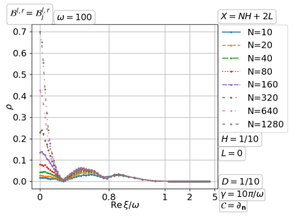
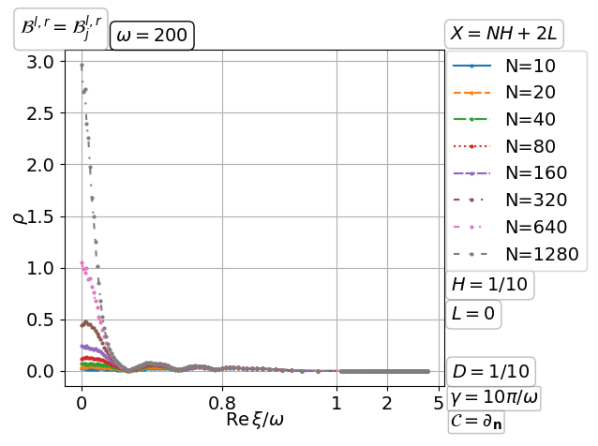
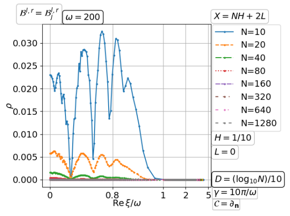
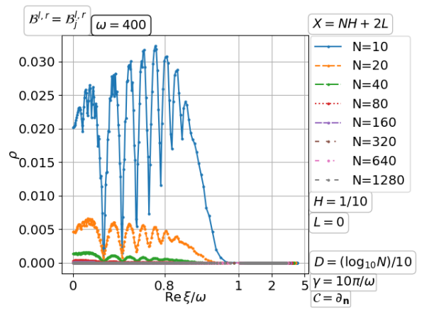
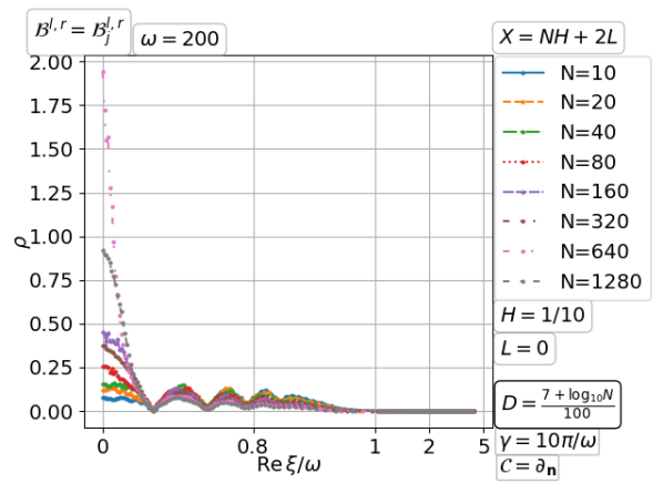
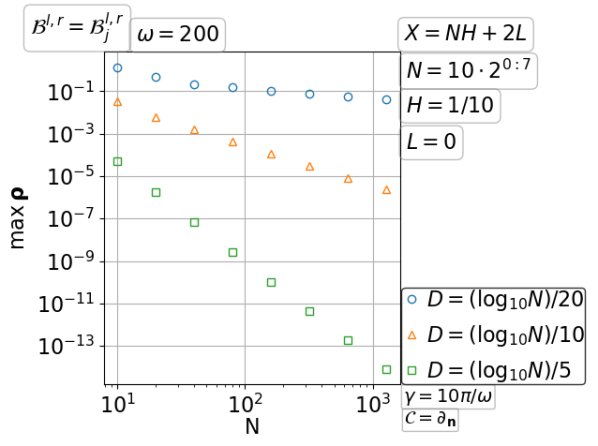
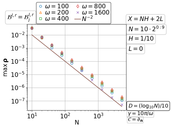
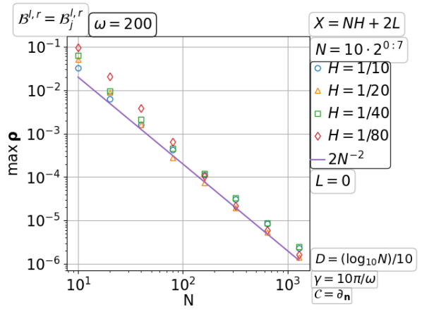
Figure 3.42: Convergence and divergence of the double sweep Schwarz method with PML transmission for the free space wave with increasing number of fixed size subdomains. (Scaling of $\max_{\xi}\rho$ not $1-\max_{\xi}\rho$!)

Convergence on a fixed domain with increasing number of subdomains

Based on the previous paragraph, we choose a sufficiently large PML width $D$ to grow logarithmically with the number of subdomains $N$, now on a fixed domain. From the top half of Figure 3.43, we can see that the convergence factor $\rho$ decreases rapidly with $N$. Increasing the wavenumber $\omega$ only introduces more oscillations and changes little the envelope profile. We next show the constant PML width $D$ can still not work; see the first subplot of the third row. In the following subplots, the tendency of $\max_{\xi}\rho\to 0$ as $N\to\infty$ is illustrated for different values of $\omega$, $D$ and the domain width $X$. Given $D=(\log_{10}N)/10$, the speed of $\max_{\xi}\rho\to 0$ is faster than quadratic for all the listed values of $\omega$ and $X$. But the speed strongly depends on $D$ because $\max_{\xi}\rho$ decays exponentially as $D$ increases.

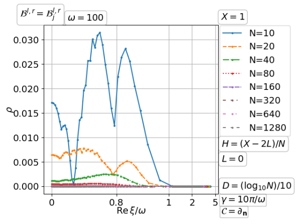
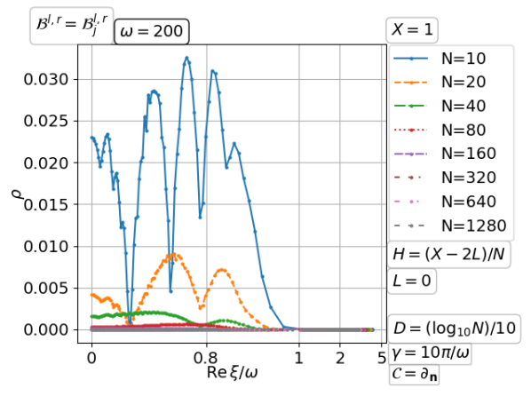
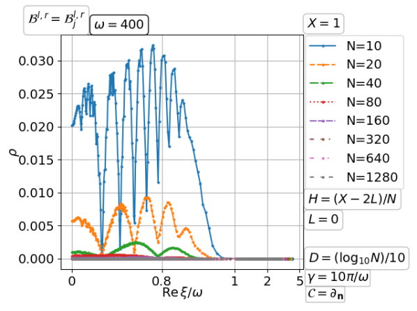
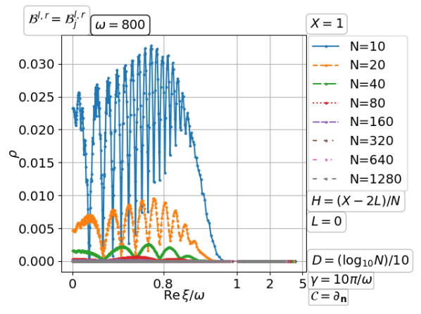
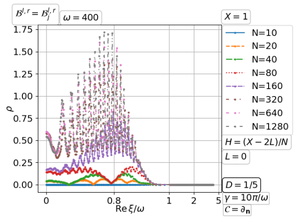
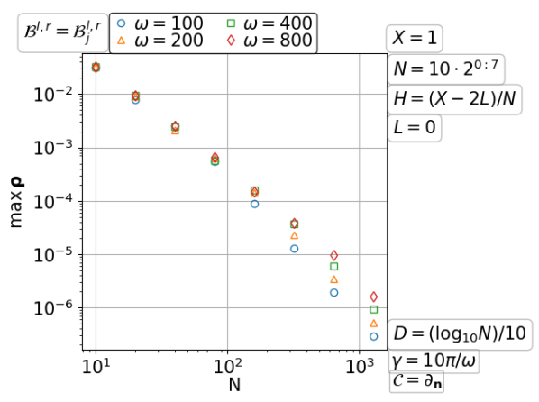
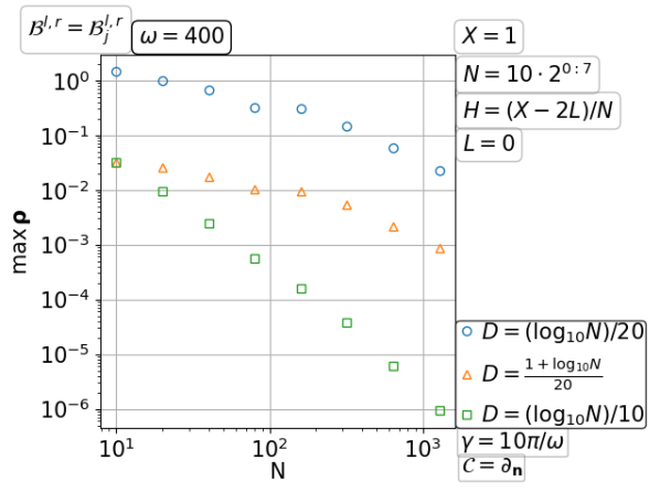
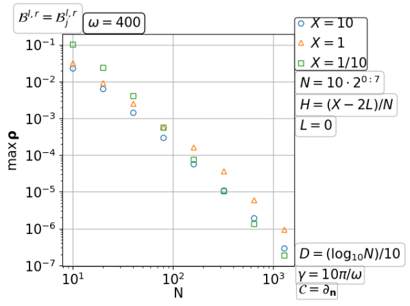
Figure 3.43: Convergence and divergence of the double sweep Schwarz method with PML transmission for the free space wave on a fixed domain with increasing number of subdomains. (Scaling of $\max_{\xi}\rho$ not $1-\max_{\xi}\rho$!)

Convergence on a fixed domain with a fixed number of subdomains for increasing wavenumber

Now we study the scaling with the wavenumber $\omega$ alone. The PML width $D$ is taken as constant with respect to $\omega$. In the top half of Figure 3.44, we see that the graph of the convergence facor $\rho=\rho(\xi)$ tends to a limiting profile as $\omega\to\infty$. So, asymptotically $\max_{\xi}\rho=O(1)$ is independent of $\omega$, as verified in the bottom half of Figure 3.44. At the same time, we see $\max_{\xi}\rho$ grows with the number of subdomains $N$, decays exponentially with $D$, and grows with shrinking domain width $X$. Moreover, we find also that $D$ needs to be sufficiently big for convergence at large $N$ and small $X$; see particularly the last subplot where divergence appears at $N=80$ and $X=1/10$.

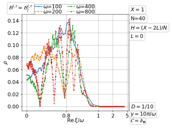
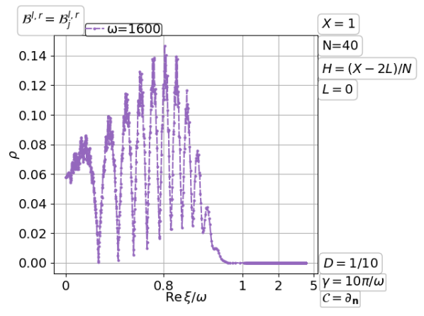
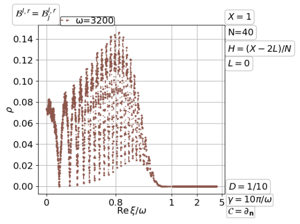
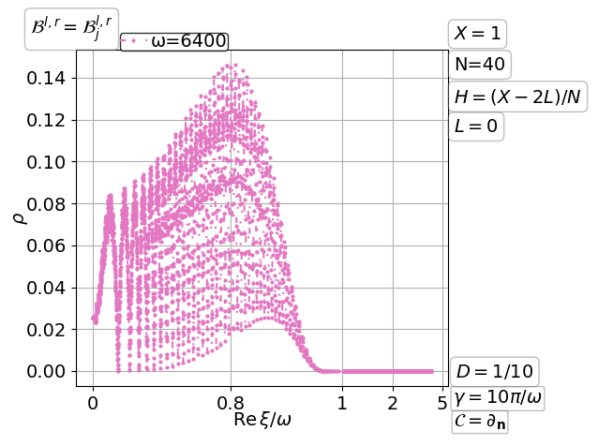
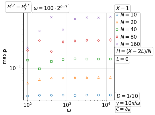
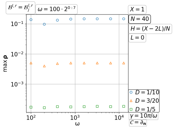
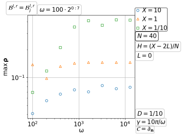
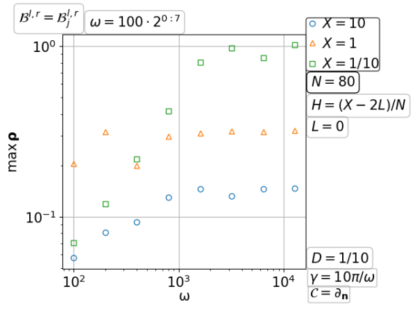
Figure 3.44: Convergence and divergence of the double sweep Schwarz method with PML transmission for the free space wave on a fixed domain with a fixed number of subdomains for increasing wavenumber. (Scaling of $\max_{\xi}\rho$ not $1-\max_{\xi}\rho$!)

Convergence on a fixed domain with number of subdomains increasing with the wavenumber

This scaling can be viewed as a combination of the previous two scalings. As learned before, a logarithmic growth of the PML width $D$ with the number of subdomains $N$ is necessary for convergence, now verified also for this scaling in the first row of Figure 3.45. Then, in the second row we see that a larger wavenumber $\omega$ causes more osciallations of the convergence factor $\rho=\rho(\xi)$ with little change of the maximum of $\rho$. Given $D=(\log_{10}N)/10$, the scaling of $\max_{\xi}\rho$ is about $O(N^{-2})$; see the bottom half of the figure. We can find that $\max_{\xi}\rho$ has a mild dependence on $\omega$ and $X$ but an exponential decay with $D$. In particular, in the third row and the last column, we see that different $D$ gives a different power law decay of $\max_{\xi}\rho$ with $N$.

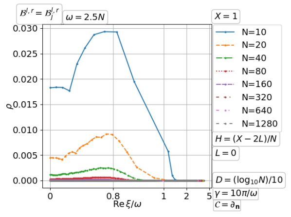
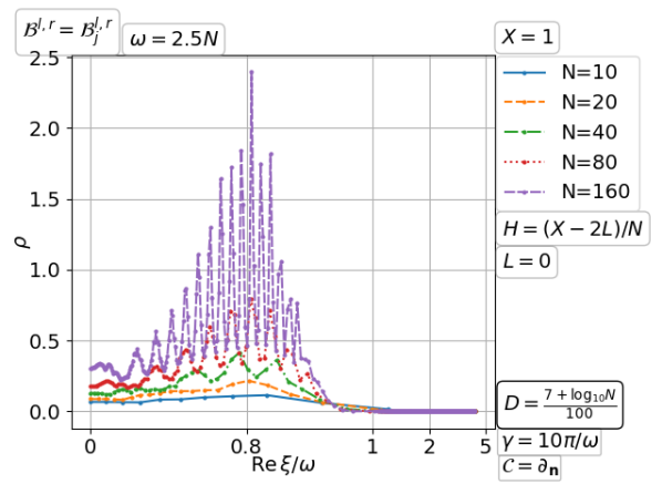
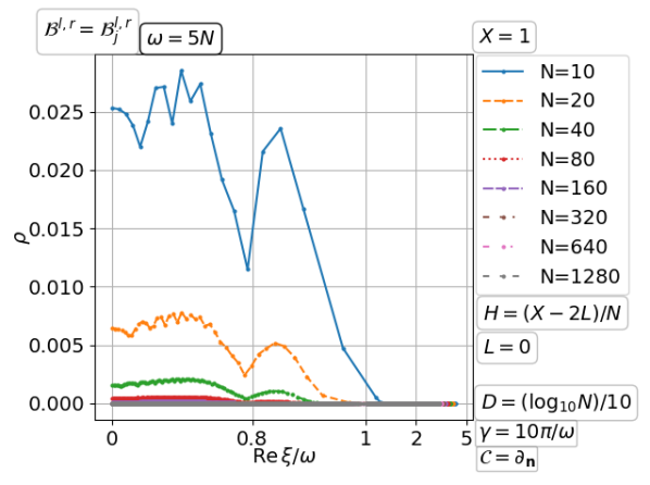
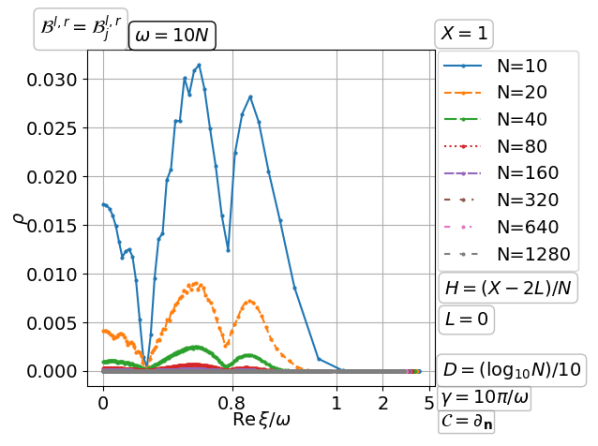
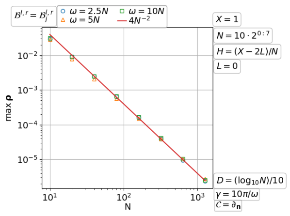
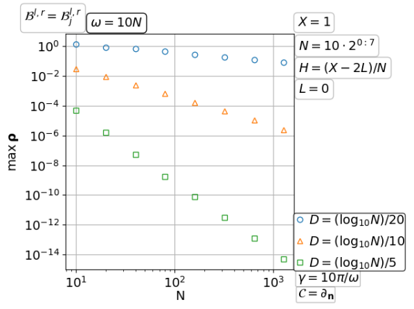
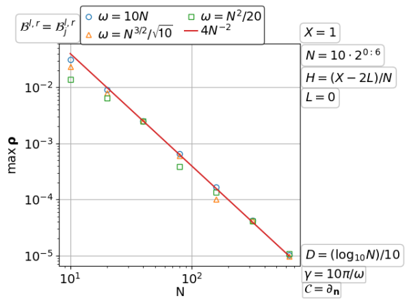
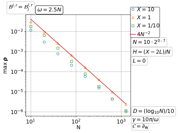
Figure 3.45: Convergence and divergence of the double sweep Schwarz method with PML transmission for the free space wave on a fixed domain with number of subdomains increasing with the wavenumber. (Scaling of $\max_{\xi}\rho$ not $1-\max_{\xi}\rho$!)

3.5 Parallel Schwarz methods for the layered medium wave problem

This case differs from the free space wave problem (see section 3.3) only in $\eta$. We assume that the inhomogeneity is bounded, the medium is layer-wise constant in a box, and the exterior medium is constant. Specifically, $\eta=-\omega^{2}/v^{2}$ with the wave velocity given as one of the following:

• or vel1($v_{1}$), one inclusion in the full space: $v=v_{1}$ when $(x,y)\in(\frac{1}{3}X,\frac{2}{3}X)\times(0,1)$, and $v=1$ on $\mathbb{R}^{2}-(\frac{1}{3}X,\frac{2}{3}X)\times(0,1)$;

• or vel2($v_{1}$), two inclusions in the full space: $v=v_{1}$ when $(x,y)\in(\frac{1}{6}X,\frac{1}{3}X)\times(0,1)$ or $(x,y)\in(\frac{2}{3}X,\frac{5}{6}X)\times(0,1)$, and $v=1$ otherwise in $\mathbb{R}^{2}$;

• or vel($l$,$v_{1}$), $l$ inclusions in the full space: $v=v_{1}$ when $(x,y)\in((j-1)W,jW)\times(0,1)$ for $j=2,4,..,2l$, $v=1$ otherwise in $\mathbb{R}^{2}$ and $W=\frac{X}{2l+1}$.

So, the medium interfaces are parallel to the subdomain interfaces. In fact, it is more favorable for convergence to choose the domain decomposition along the other direction such that the subdomain interfaces are perpendicular to the medium interfaces. But in practical applications, it is very possible to have the situation that we choose to study here. For example, if the top and bottom boundary conditions are Neumann or Dirichlet, a decomposition along the other direction will be hard for convergence. Moreover, a velocity model may contain horizontal, vertical and curved interfaces along different directions, which makes reflections traveling back and forth between subdomains unavoidable.

Numerical experiments of the double sweep Schwarz method with a matrix Schur complement transmission based on the constant-medium extension have shown the difficulty of convergence in layered media (?). An analysis and approximation of the variable-medium Dirichlet-to-Neumann operator is carried out by ?, and more recently they proposed a matrix optimization approach to the infinite element method (?, ?). A boundary integral transmission condition is proposed by ?. The idea of ? consists in extending each layer (used as subdomain) to a slab in the physical domain, which can be thought as using a physical PML, and approximately solving the extended subdomain problem (with zero source in the extension) by a fast direct solver. The impact of reflected waves in the direction of decomposition was early recognized by ? for the PML transmission, see also ?.

Our goal in this subsection is to explore the convergence factor $\rho$ based on the Fourier analysis, as we did in the previous part of this review. A main difference in this case is that the interface-to-interface operators $a_{j}$, $b_{j}$, $c_{j}$, $d_{j}$ need to be solved from subdomain layered medium problems. In this case, Taylor of order zero transmission with overlap can diverge for some medium distribution, and without overlap it hardly gives good convergence, albeit it does converge without overlap when $\mathcal{B}^{r}_{j}=\mathcal{B}_{j+1}^{l}$ as guaranteed by ?. The situation can be improved by using relaxation and nonlocal transmission conditions (?). For simplicity, we will focus on the PML transmission which has been numerically tested for layered media problems (?, ?, ?).

Convergence with increasing number of fixed size layers as subdomains

We use medium layers as subdomains. So, the subdomain interfaces are aligned with the medium interfaces. It is then a question which wave velocity to take in the PML equation along an interface. In Figure 3.46 (except the last subplot), the same PML Dirichlet-to-Neumann is used for $\mathcal{B}_{j}^{r}$ and $\mathcal{B}_{j+1}^{l}$, and in particular, the domain averaged velocity $\bar{v}=\frac{1}{|\Omega|}\int_{\Omega}v$ is used in all the PML equations. The choice of $\mathcal{B}_{j}^{r}=\mathcal{B}_{j+1}^{l}$ here seems important for convergence, as emphasized in general convergence proofs of parallel optimized Schwarz methods without overlap (?, ?). For example, if we take the wave velocity in the right neighborhood of $\{X_{j}^{r}\}\times(0,Y)$ for $\mathcal{B}_{j}^{r}$ but the wave velocity in the left neighborhood of $\{X_{j+1}^{l}\}\times(0,Y)$ for $\mathcal{B}_{j+1}^{l}$, we will get divergence no matter how large or strong a PML is used, see the last subplot of Figure 3.46. In the top half of Figure 3.46, the graphs of $\rho=\rho(\xi)$ tell us roughly that lower frequency modes converge slower, higher contrast in the wave velocity leads to slower convergence for modest number of subdomains $N$, and increasing PML width $D$ has a limited positive impact on convergence of low frequency modes. In the following three subplots, the scaling of $1-\max_{\xi}\rho$ with $N$ and its dependence on $\omega$, $D$ and contrast in the wave velocity $v_{1}$ are illustrated. Specifically, $1-\max_{\xi}\rho$ decreases with $N$ almost independently of $\omega$ for an initial stage and then stays at a constant which comes later for larger $\omega$.

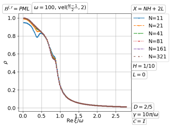
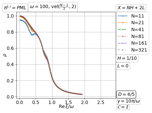
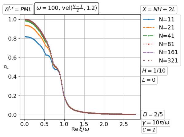
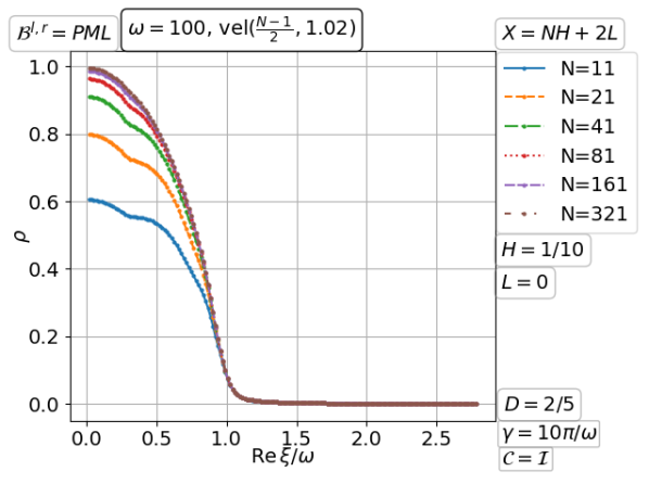
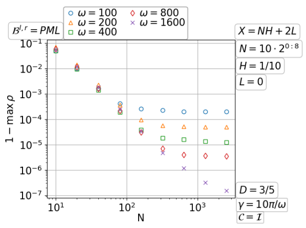
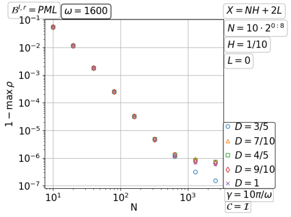
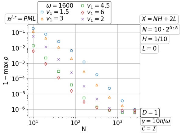
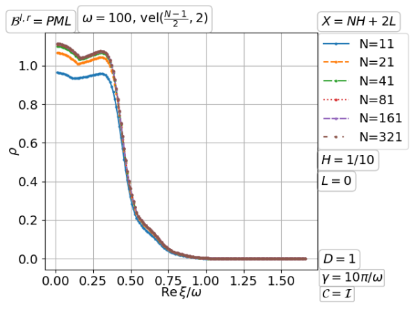
Figure 3.46: Convergence ($\mathcal{B}_{j}^{r}=\mathcal{B}_{j+1}^{l}$ except bottom right) and divergence ($\mathcal{B}_{j}^{r}\neq\mathcal{B}_{j+1}^{l}$ bottom right) of the parallel Schwarz method with PML transmission for the full space wave problem with fixed size medium layers as subdomains.

Convergence on a fixed domain with increasing number of subdomains

In this case, the medium property in the domain is also fixed as we increase the number of subdomains. The subdomain interfaces are not aligned with the medium interfaces. Here, it turns out not to be a good idea (divergence observed) to take the domain average wave velocity as we did in the last paragraph. Instead, we simply use the values of the wave velocity at subdomain interfaces for the PML equations. Figure 3.47 compares the ‘vel1’ and ‘vel2’ velocity models in two columns. It can be seen that the convergence for ‘vel2’ is slower than for ‘vel1’. Their convergence rates $\max_{\xi}\rho$ both deteriorate to $1$ linearly with $N^{-1}\to 0$ but are independent of $\omega$. The convergence also deteriorates with higher contrast in the wave velocity $v_{1}$. Roughly, $1-\max_{\xi}\rho$ looks like $O(v_{1}^{-1})$ for ‘vel1’ and $O(v_{1}^{-2})$ for ‘vel2’.

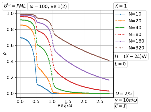
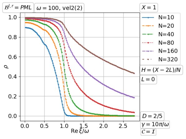
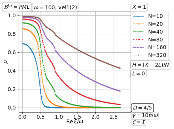
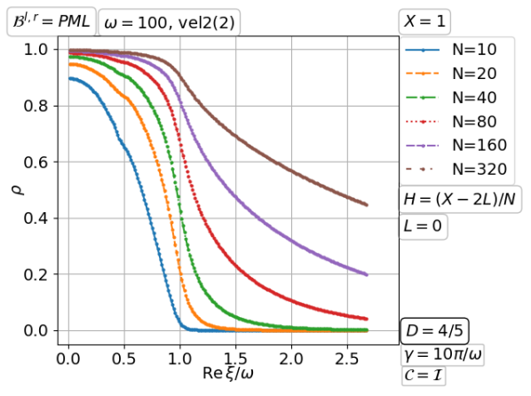
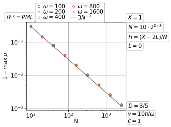
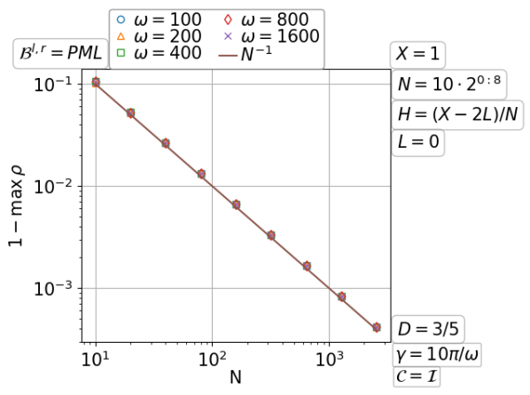
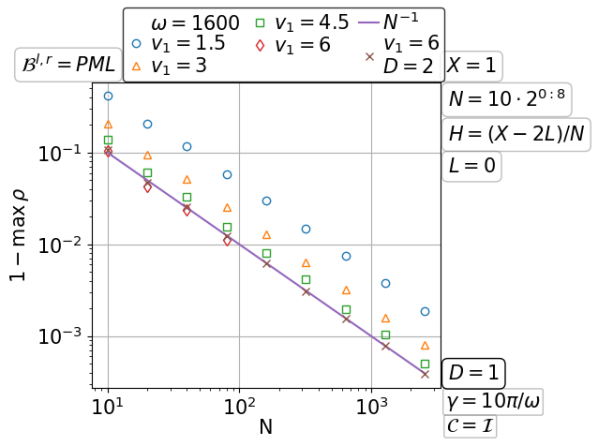
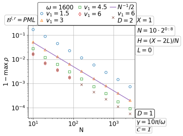
Figure 3.47: Convergence of the parallel Schwarz method with PML transmission for the full space wave problem with one inclusion (left) and two inclusions (right) on a fixed domain with increasing number of subdomains.

3.6 Double sweep Schwarz methods for the layered medium wave problem

As seen in the constant medium case, Taylor of order zero transmission can hardly work with the double sweep iteration. So, we will focus solely on the PML transmission. The readers are referred to the beginning part of the previous subsection for the velocity models used here.

Convergence and divergence with increasing number of fixed size layers as subdomains

In this case, we found it is better to use the neighbor’s wave velocity for the PML equation of a subdomain. But even for this choice, divergence is observed for a large number of layers (as subdomains); see Figure 3.48.

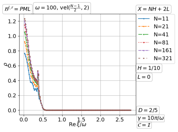
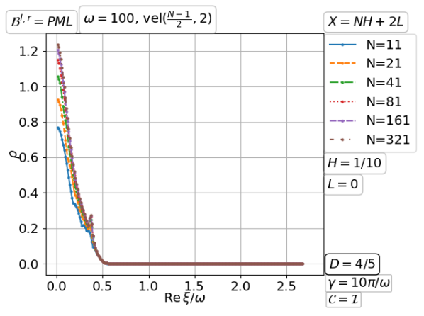
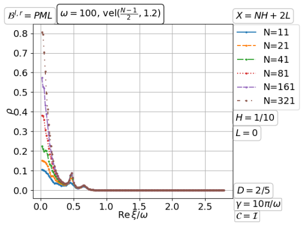
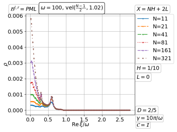
Figure 3.48: Convergence and divergence of the double sweep Schwarz method with PML transmission for the full space wave problem with fixed size medium layers as subdomains.

Convergence on a fixed domain with increasing number of subdomains

Compared to the parallel iteration previously shown in Figure 3.47, the double sweep iteration converges significantly faster (see Figure 3.49) and does not seem to deteriorate with a larger number of subdomains $N$. For ‘vel1’, the convergence rate $\max_{\xi}\rho$ is independent of the wavenumber $\omega$. But for ‘vel2’, $\max_{\xi}\rho$ oscillates with $\omega$. Higher contrast in the wave velocity $v_{1}$ leads to slower convergence. In the bottom right subplot, we see a deterioration of the convergence factor when the inclusions become smaller and more, and in particular divergence with more than three inclusions.

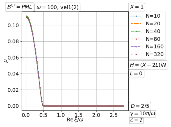
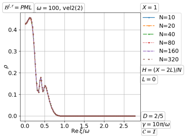
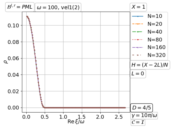
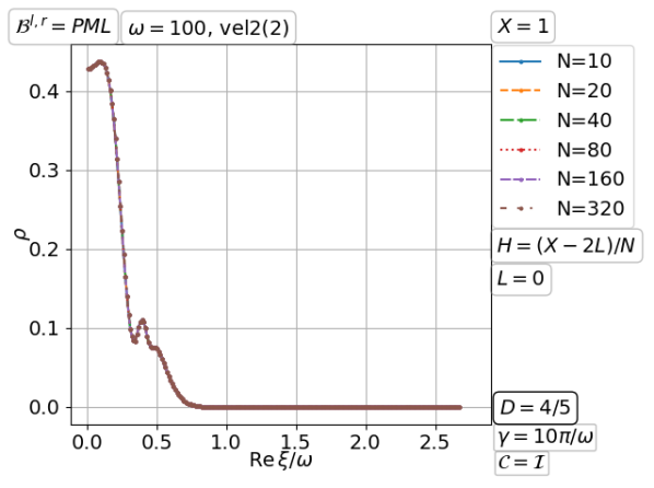
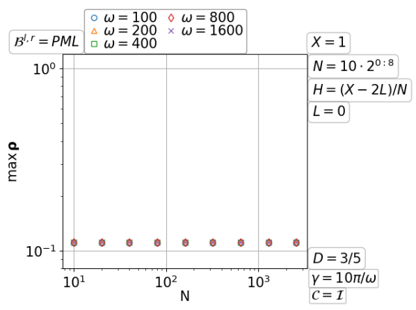
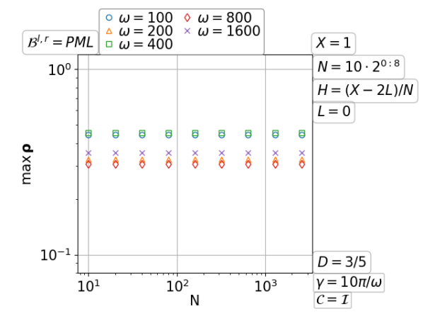
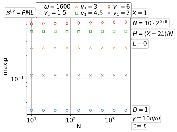
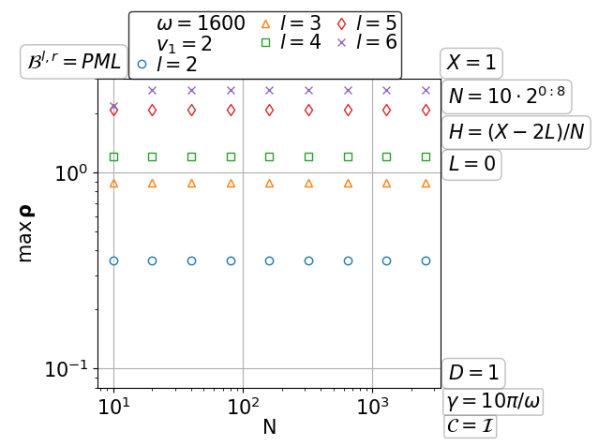
Figure 3.49: Convergence of the double sweep Schwarz method with PML transmission for the full space wave problem with one inclusion (left), two inclusions (right except bottom) and $l$ inclusions (bottom right) on a fixed domain with increasing number of subdomains. (Scaling of $\max_{\xi}\rho$ not $1-\max_{\xi}\rho$!)

With these results and the results in the previous subsection on layered medium wave problems, we have seen the limitations of PML transmission conditions. Is there a better way? For example, are the nonlocal transmission conditions (?) or the learned infinite elements (?, ?) more robust for layered media? To what extent can PML work for general variable media problems? For example, how to explain the success seen in the existing literature for numerous geophysical applications? Can other techniques be combined with transmission conditions as a remedy? We emphasize the recent progress of some techniques for solving wave problems: for example, coarse spaces (?, ?, ?) or deflation (?, ?, ?), time domain solvers (?, ?, ?, ?), absorption or shifted-Laplace (?, ?, ?, ?), $\mathcal{H}$-matrix (?, ?, ?, ?), DPG (?) and high-frequency asymptotic (?, ?, ?). There are plenty of questions still to be answered in the future.

4 Schwarz methods with cross points

In a domain decomposition, a cross point is where more than two subdomains intersect. If a cross point is on the boundary of a subdomain, a transmission pattern thereof has to be decided. This is important especially at the discrete level when the cross point is associated with a degree of freedom. For detailed discussions, see ?, ?, ?. In particular, different treatments of cross points for high-order (e.g. PML) transmission conditions have recently been proposed by ?, ?, ?, ?, ?. See also ?, ? for nonlocal transmission conditions. A related issue is to deal with a corner point where the normal direction is not unique (?, ?, ?).

Our emphasis in this section is on optimal Schwarz methods that converge exactly in finite steps, i.e. methods that are nilpotent. But before that, we mention quickly a couple of workable treatments of cross points in a general decomposition that are practically useful albeit non-optimal.

From the viewpoint of the subdomain boundary, a cross point is where the interfaces of the subdomain with two different neighbors join. In a non-overlapping decomposition, a simple approach is to include the cross point for transmission on both the interfaces with the two neighbors. For example, in the non-overlapping case ($\Omega_{ij}=\tilde{\Omega}_{ij}$) of the decomposition in Figure 1.2 (left), the method of ? for the time-harmonic wave problem $(-\Delta+\omega^{2})u=f$ in $\Omega$ uses $(-\partial_{x}+\I\,\omega)u_{ij}=(-\partial_{x}+\I\,\omega)u_{i-1,j}$ on $\{X_{i}^{l}\}\times[Y_{j}^{b},Y_{j}^{t}]$ and $(-\partial_{y}+\I\,\omega)u_{ij}=(-\partial_{y}+\I\,\omega)u_{i,j-1}$ on $[X_{i}^{l},X_{i}^{r}]\times\{Y_{j}^{b}\}$, and any degrees of freedom associated with the cross point at $(X_{i}^{l},Y_{j}^{b})$ will be taken into account for both of the transmission conditions. In the substructured form of the Schwarz method that reduces the unkowns to the interfaces, this cross point treatment means introducing an unknown (data for the transmission condition, also called dual variable or Lagrange multiplier) at the cross point for each incident interface of the subdomain. Another approach is to keep the original degrees of freedom (also called primal variables) and the corresponding equations at cross points unique (unsplit), then separate them out by a Schur complement from the other primal and the dual variables (?).

In an overlapping decomposition, the interfaces of a subdomain with its different neighbors can overlap. To avoid redundant transmission, a partition of unity of the subdomain boundary is used. A very natural choice is from a non-overlapping decomposition of the domain. For example, in Figure 1.2 we can take $\partial\Omega_{ij}\cap\tilde{\Omega}_{i-1,j}$ as the interface for transmission to $\Omega_{ij}$ from $\Omega_{i-1,j}$. But cross points where two interfaces of a subdomain join still exist. For example, in Figure 1.2, we have the cross point where $\partial\Omega_{ij}\cap\overline{\tilde{\Omega}}_{i-1,j}$ joins with $\partial\Omega_{ij}\cap\overline{\tilde{\Omega}}_{i-1,j-1}$. At the discrete level, one can still assign the cross point uniquely to one of the incident interface, and there is no problem for the implementation of Schwarz methods based on subdomain iterates or interface substructuring. The deferred correction form provides another approach, which starts from an initial guess (or the previous iterate) of the solution on the original domain, takes the residual to subdomains for local corrections, and make a global correction by gluing the local corrections. To minimise communication between subdomains, it is practically common to use a non-overlapping decomposition of the domain for gluing the local corrections, which gives the Restricted Additive Schwarz (RAS) method proposed by ? with Dirichlet transmission conditions, and the Optimized Restricted Additive Schwarz (ORAS) method proposed by ?, with general Robin-like interface conditions. Moreover, it was shown in ? that, under some algebraic assumptions on the gluing scheme, ORAS is equivalent to the parallel Schwarz method with the corresponding transmission conditions. In the case of non-equivalence, the transmission data coming from the glued global iterate can be a mix of multiple subdomain solutions. However, there is no convergence theory (except using the maximum principle) for RAS and ORAS as of today. ? analyzed a symmetrised version of RAS and ORAS using the same non-overlapping partition-of-unity for both the restriction/prolongation operators. ? analyzed a symmetrised optimized Schwarz method for the Helmholtz equation. See ?, ? for more analysis of symmetrised Schwarz preconditioners for indefinite problems.

Now we turn to the main question: is there an optimal Schwarz method beyond the sequential decomposition? For example, Figure 1.2 (right) is a sequential decomposition and Figure 1.2 (left) is not. A difficulty arises even in Figure 1.2 (right) when the domain is $X$-periodic in $x$, then the first subdomain is coupled to the last subdomain by identifying the boundary $\{0\}\times[0,Y]$ with $\{X\}\times[0,Y]$. The difficulty is that an interface $\{X_{i}^{l}\}\times[0,Y]$ can not separate the original problem into two regions because the region on the left is coupled to the region on the right not only through the interface but also through the periodic condition. Similarly, an annular domain decomposed into annular sectors has the same problem. The issue from a loop of subdomains was recognized early by ?. It arises also in a decomposition with cross points; as posed by ?. For example, in Figure 1.2 (left) the interface $\{X_{i}^{l}\}\times[Y_{j}^{b},Y_{j}^{t}]$ can not separate the domain into two regions because there is also a loop in the subdomain adjacency relation. Why do we need an interface separating the domain into two regions? Because that is the case for the domain truncation and transmission to work as in the sequential decomposition.

The key of domain truncation and transmission can be understood in analogy to Gaussian elimination. If there is no source term in the complementary domain of a subdomain, one needs only to approximate the Schur complement which corresponds to a transparent boundary condition along the interface separating the subdomain and its complementary domain, such that the subdomain solution coincides with the solution of the original problem. If there is a source in the complementary domain, one needs only to know the solution corresponding to the source in an arbitrarily small outer (viewed from the subdomain) neighborhood of the interface, and to take the outer source into the subdomain through a transmission condition (conveniently using the same boundary operator as in the transparent boundary condition), which is like a back substitution in Gaussian elimination.

So, how did the recent work of ?, ? revive the domain truncation and transmission in a checkerboard decomposition like Figure 1.2 (left)? To understand their idea which is truly creative and a big step from the formerly existing optimal Schwarz methods, it is very worth to read the original work. In this review, we present what we have learned. First, it is good to have conceptually a domain truncation of the original problem into a patch including the target subdomain, and use the truncated problem on the patch for transmission into the subdomain. For example, in Figure 1.2 (left), a patch including $\Omega_{ij}$ can be $\Xi_{i,j}^{l}:=\bar{\Omega}_{1j}\cup\cdots\cup\bar{\Omega}_{ij}$. A PML surrounding $\Xi_{i,j}^{l}$ is used for domain truncation of the original problem, and we denote the PML augmented patch by $\hat{\Xi}_{ij}^{l}$. Note that $\Omega_{ij}$ is also augmented with PML for domain truncation of the original problem, and the PML augmented subdomain is denoted by $\hat{\Omega}_{ij}$. A transmission will take place through the interface $\hat{\Gamma}_{ij}^{l}:=\hat{\Omega}_{ij}\cap\{(x,y):x=X_{i}^{l}\}$. Let $\hat{\Omega}_{ij}^{l}:=\hat{\Omega}_{ij}\cap\{(x,y):x\geq X_{i}^{l}\}$. We assume the PML on top (and bottom) of $\Xi_{1j}$, $\Xi_{2j}$, …, $\Omega_{1j}$, $\Omega_{2j}$, … are conforming (i.e., the same) along their interfaces and in their overlaps, and the PML on the right of $\Xi_{ij}^{l}$ and $\Omega_{ij}$ are also the same. In the following lemma, we show conceptually how the sources on the left of $\Omega_{ij}$ can be transmitted into $\Omega_{ij}$.

Lemma 4.1

Suppose the source $f$ of the original problem eqprb vanishes on $(X_{i}^{l},X]\times[0,Y]$ and $[0,X]\times([0,Y]-[Y_{j}^{b},Y_{j}^{t}])$; see Figure 4.1. Let $\hat{v}_{ij}^{l}$ be the solution of the truncated problem on $\hat{\Xi}_{ij}^{l}$. Let $\hat{u}_{ij}^{l}$ be the solution of

$$(\mathcal{L}_{x}+\mathcal{L}_{y}+\eta)\hat{u}_{ij}^{l} =0 \text{ on }\hat{\Omega}_{ij}^{l},$$ (57)

$$\mathcal{C}\hat{u}_{ij}^{l} =0 \text{ on }[X_{i}^{l},X_{i}^{r}+D]\times\{Y_{j}^{b}-D,Y_{j}^{t}+D\},$$

$$\mathcal{C}\hat{u}_{ij}^{l} =0 \text{ on }\{X_{i}^{r}+D\}\times[Y_{j}^{b}-D,Y_{j}^{t}+D],$$

$$\mathcal{B}\hat{u}_{ij}^{l} =\mathcal{B}\hat{v}_{ij}^{l} \text{ on }\hat{\Gamma}_{ij}^{l}=\{X_{i}^{l}\}\times[Y_{j}^{b}-D,Y_{j}^{t}+D],$$

where $\mathcal{C}$ is the terminating condition of the PML, and $\mathcal{B}$ is any boundary operator that makes the problem well-posed. Then, $\hat{u}_{ij}^{l}$ equals the restriction of $\hat{v}_{ij}^{l}$ onto $\hat{\Omega}_{ij}^{l}$.

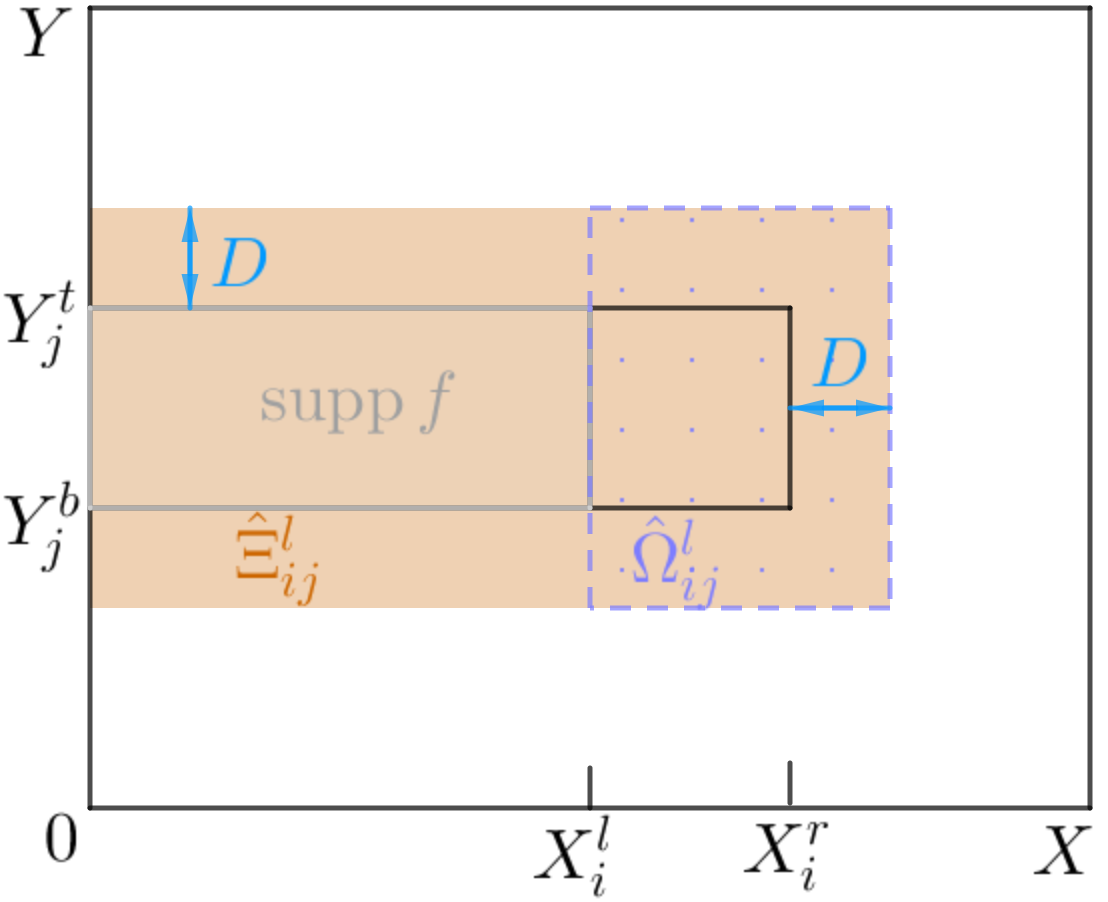
Figure 4.1: Illustration of Lemma 4.1 for the transmission in the patch $\hat{\Xi}_{ij}^{l}$.

Proof 4.2.

Since eqtl has the unique solution $\hat{u}_{ij}^{l}$ and the restriction of $\hat{v}_{ij}^{l}$ onto $\hat{\Omega}_{ij}^{l}$ satisfies eqtl, the two must be equal.

Remark 4.3.

If the PML of $\hat{\Xi}_{ij}^{l}$ is exactly transparent, then the restriction of $\hat{v}_{ij}^{l}$ onto $\Xi_{ij}^{l}$ coincides with the solution of the original problem, and so is the restriction of $\hat{u}_{ij}^{l}$ onto $\Omega_{ij}$. A transparent PML does exist at the continuous level, see e.g. ?.

Remark 4.4.

To solve eqtl, we need only the knowledge of $\hat{v}_{ij}^{l}$ in a left neighborhood of $\hat{\Gamma}_{ij}^{l}$ to evaluate the transmission data $\mathcal{B}\hat{v}_{ij}^{l}$. The truncated problem on the patch $\hat{\Xi}_{ij}^{l}$ is never solved directly (like the original problem on $\Omega$ is never solved directly). In the algorithm to be detailed later, the transmission data is obtained from a solution defined on $\hat{\Omega}_{i-1,j}$. In a deferred correction form, the residual instead of the transmission data is evaluated, which gives rise to the source transfer method (?); see ? for their relation.

Remark 4.5.

Since we also want to resolve the local source $f_{ij}$ – the restriction of $f$ onto ${\Omega}_{ij}$, the truncated problem on $\hat{\Omega}_{ij}$ will be used. It is then convenient to take $\mathcal{B}$ as $-\partial_{x}+\mathcal{S}$ with $\mathcal{S}$ the PML Dirichlet-to-Neumann operator eqsd or eqsw defined by the PML $\hat{\Omega}_{ij}-\hat{\Omega}_{ij}^{l}$. In this case, the problem eqtl is extended to $\hat{\Omega}_{ij}$ with $\mathcal{S}$ unfolded (?).

Remark 4.6.

Note that we can replace in Lemma 4.1 the patch and the subdomain with an arbitrary domain $\Xi$ and an arbitrary subdomain $\Omega_{*}\subset\Xi$ of any shape, with the transmission condition put on $\partial\Omega_{*}-\partial\Xi$ and the source $f$ vanishing on $\Omega_{*}$, as long as the problems on $\Xi$ and $\Omega_{*}$ are well-posed. See also ? for the source transfer version.

Similarly, we can define the patches $\Xi_{ij}^{r}$, $\Xi_{ij}^{t}$, $\Xi_{ij}^{b}$ for the transmission of the sources outside the right/top/bottom of $\Omega_{ij}$; see Figure 4.2 (left). There are still four corner regions outside $\Omega_{ij}$. For the source to the bottom left of $\Omega_{ij}$, we have conceptually the patch $\Xi_{ij}^{bl}:=\cup_{{c\leq i;\ r\leq j}}\bar{\Omega}_{cr}$ and the PML augmented patch $\hat{\Xi}_{ij}^{bl}$; see Figure 4.2 (right). Let $\hat{\Omega}_{ij}^{bl}:=\hat{\Omega}_{ij}\cap\{(x,y):x\geq X_{i}^{l},y\geq Y_{j}^{b}\}$. A transmission will take place through the interface $\hat{\Gamma}_{ij}^{bl}:=\hat{\Omega}_{ij}\cap\partial\hat{\Omega}_{ij}^{bl}$. Although the source to be transmitted into $\Omega_{ij}$ is to the bottom left of $\Omega_{ij}$, i.e., on $\Xi_{i-1,j-1}^{bl}$, a patch containing both $\Omega_{ij}$ and $\Xi_{i-1,j-1}^{bl}$ has to be larger for the PML to work. That is why the patch $\Xi_{ij}^{bl}$ is used. As we mentioned in the above remarks following Lemma 4.1, the PML augmented problem on $\hat{\Omega}_{ij}$ can be solved with either the transmission data on $\hat{\Gamma}_{ij}^{bl}$ or the residual in a top-right neighborhood of $\hat{\Gamma}_{ij}^{bl}$ which in turn is acquired from a glued version of subdomain solutions on $\Omega_{i-1,j}$, $\Omega_{i-1,j-1}$ and $\Omega_{i,j-1}$. The resulting solution $\hat{u}_{ij}^{bl}$ on $\hat{\Omega}_{ij}$ then has the same restriction onto $\hat{\Omega}_{ij}^{bl}$ as does the conceptual solution $\hat{v}_{ij}^{bl}$ for the source located to the bottom left of $\Omega_{ij}$. In the same way, we can define the PML augmented patches $\hat{\Xi}_{ij}^{br}$, $\hat{\Xi}_{ij}^{tr}$, $\hat{\Xi}_{ij}^{tl}$ for the transmission of the sources located to the bottom-right/top-right/top-left of $\Omega_{ij}$.

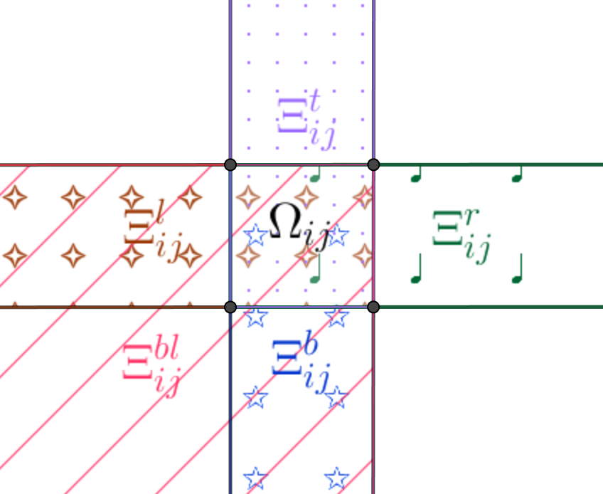
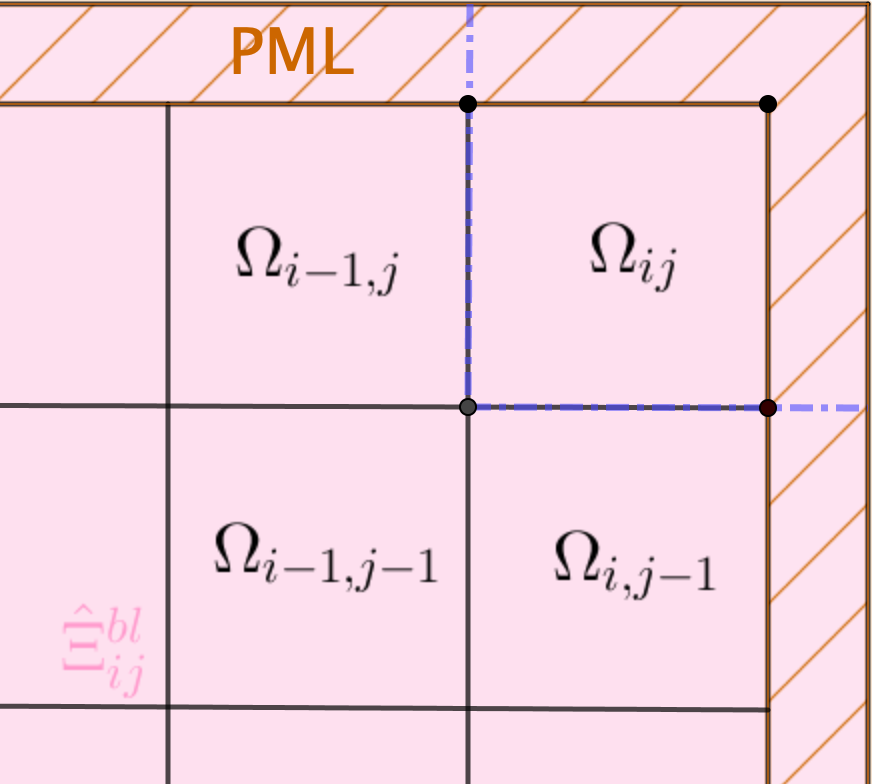
Figure 4.2: Patches containing the target subdomain $\Omega_{ij}$ (left), and the bottom left patch augmented with PML $\hat{\Xi}_{ij}^{bl}$ for the non-overlapping decomposition (right).

Let $\hat{u}_{ij}^{c}$ be the solution of the truncated problem on $\hat{\Omega}_{ij}$ corresponding to the original problem eqprb with the source $f$ vanishing outside $\Omega_{ij}$. Clearly, if we have the solutions $\hat{u}_{ij}^{l,r,b,t,bl,br,tl,tr,c}$ and the PML is exactly transparent, then their sum on $\Omega_{ij}$ equals the solution of the original problem with the source $f$ distributed anywhere on $\Omega$, based on the linearity of eqprb. The remaining question is how to get the transmission data needed for $\hat{u}_{ij}^{l,r,b,t,bl,br,tl,tr}$ on $\hat{\Omega}_{ij}$. This is based on the following induction on the subscripts $i$, $j$. Only the transmission data for $\hat{u}_{ij}^{l,bl}$ are illustrated.

Lemma 4.7.

Let the domain decomposition be non-overlapping. Suppose the PML is exactly transparent and the solutions $\hat{u}_{i-1,j}^{l,c}$ are available on $\hat{\Omega}_{i-1,j}$. Let $\hat{\Omega}_{i-1,j}^{lr}:=\hat{\Omega}_{i-1,j}\cap\{(x,y):X_{i-1}^{l}\leq x\leq X_{i-1}^{r}\}$. Then $\hat{u}_{i-1,j}^{l}+\hat{u}_{i-1,j}^{c}$ and $\hat{v}_{i,j}^{l}$ have the same restriction onto $\hat{\Omega}_{i-1,j}^{lr}$ and in particular the same trace $\mathcal{B}\hat{v}_{i,j}^{l}$ on $\hat{\Gamma}_{ij}^{l}$ for any boundary operator $\mathcal{B}$.

Proof 4.8.

By Lemma 4.1, $\hat{u}_{i-1,j}^{l}$ coincides with $\hat{v}_{i-1,j}^{l}$ on $\hat{\Omega}_{i-1,j}^{l}\supset\hat{\Omega}_{i-1,j}^{lr}$. Let $\hat{V}_{ij}^{l}$ be the solution operator taking a source in $\Xi_{ij}^{l}$ as input for the truncated problem on $\hat{\Xi}_{ij}^{l}$. Let $\chi_{i-1,j}$ be the indicator function of $\Omega_{i-1,j}$. Let $f$ be the source in $\Xi_{i-1,j}^{l}$ (the domain on the left side of $\Omega_{ij}$) for obtaining $\hat{v}_{ij}^{l}$. Then, $f=\chi_{i-1,j}f+(1-\chi_{i-1,j})f$ and $\hat{v}_{ij}^{l}=\hat{V}_{ij}^{l}(\chi_{i-1,j}f)+\hat{V}_{ij}^{l}((1-\chi_{i-1,j})f)$. Since the PML is exact, $\hat{u}_{i-1,j}^{c}=\hat{V}_{ij}^{l}(\chi_{i-1,j}f)$ and $\hat{v}_{i-1,j}^{l}=\hat{V}_{ij}^{l}((1-\chi_{i-1,j})f)$ on $\hat{\Omega}_{i-1,j}^{lr}$. Hence, $\hat{u}_{i-1,j}^{c}+\hat{u}_{i-1,j}^{l}=\hat{v}_{ij}^{l}$ on $\hat{\Omega}_{i-1,j}^{lr}$.

Remark 4.9.

Since we rely on the linearity or superposition principle, we need a partition of unity to restrict the source to the non-overlapping subdomains. So the source across the interfaces needs to be treated carefully. For a square integrable source, the partition is naturally done by the variational form. For a singular source e.g. Dirac line source or point source on the interface, one needs to split the source, e.g., regard the source belonging to the subdomain on the left of the interface. Similarly, the source at a cross point needs a careful partition of unity.

Lemma 4.10.

Let the domain decomposition be non-overlapping. Suppose the PML is exactly transparent and the solutions $\hat{u}_{i-1,j}^{b,bl}$ on $\hat{\Omega}_{i-1,j}$, $\hat{u}_{i,j-1}^{l,bl}$ on $\hat{\Omega}_{i,j-1}$ and $\hat{u}_{i-1,j-1}^{l,b,bl,c}$ on $\hat{\Omega}_{i-1,j-1}$ are given. Let $\hat{\Omega}_{i-1,j}^{lrb}:=\hat{\Omega}_{i-1,j}\cap\{(x,y):X_{i-1}^{l}\leq x\leq X_{i-1}^{r},y\geq Y_{j}^{b}\}$ and $\hat{\Omega}_{i,j-1}^{lbt}:=\hat{\Omega}_{i,j-1}\cap\{(x,y):x\geq X_{i}^{l},Y_{j-1}^{b}\leq y\leq Y_{j-1}^{t}\}$. Then $\hat{u}_{i-1,j}^{b}+\hat{u}_{i-1,j}^{bl}=\hat{v}_{i,j}^{bl}$ on $\hat{\Omega}_{i-1,j}^{lrb}$, $\hat{u}_{i,j-1}^{l}+\hat{u}_{i,j-1}^{bl}=\hat{v}_{i,j}^{bl}$ on $\hat{\Omega}_{i,j-1}^{lbt}$, and $\hat{u}_{i-1,j-1}^{l}+\hat{u}_{i-1,j-1}^{b}+\hat{u}_{i-1,j-1}^{bl}+\hat{u}_{i-1,j-1}^{c}=\hat{v}_{i,j}^{bl}$ on $\Omega_{i-1,j-1}$.

Proof 4.11.

Similar to the proof of Lemma 4.7, so the details are omitted.

Remark 4.12.

Based on Lemma 4.10, the solutions $\hat{u}_{i-1,j}^{b}+\hat{u}_{i-1,j}^{bl}$, $\hat{u}_{i,j-1}^{l}+\hat{u}_{i,j-1}^{bl}$ and $\hat{u}_{i-1,j-1}^{l}+\hat{u}_{i-1,j-1}^{b}+\hat{u}_{i-1,j-1}^{bl}+\hat{u}_{i-1,j-1}^{c}$ can be glued along the interfaces by a partition of unity to a function on the L-shaped block $\overline{\hat{\Omega}_{i-1,j}^{lrb}}\cup\overline{\hat{\Omega}_{i,j-1}^{lbt}}\cup\overline{\Omega_{i-1,j-1}}$ which equals $\hat{v}_{ij}^{bl}$. Then, the function can be used for evaluation of the transmission data or residual.

Now we can present the L-(diagonal) sweep preconditioner of ?, ?, ?. For simplicity, let us consider a non-overlapping decomposition with $3\times 3$ subdomains. In the following we first list the steps corresponding to a sweep from bottom left to top right.

• For each $(i,j)$, solve the truncated problem on $\hat{\Omega}_{ij}$ with the local source $f$ restricted onto $\Omega_{ij}$, and denote the solution by $\hat{u}_{ij}^{c}$.

• Solve for $\hat{u}_{21}^{l}$ on $\hat{\Omega}_{21}$ and $\hat{u}_{12}^{b}$ on $\hat{\Omega}_{12}$ with the transmission data provided by $\hat{u}_{11}^{c}$.

• Solve for $\hat{u}_{31}^{l}$ on $\hat{\Omega}_{31}$, $\hat{u}_{13}^{b}$ on $\hat{\Omega}_{13}$ and $\hat{u}_{22}^{l,b,bl}$ on $\hat{\Omega}_{22}$ with the transmission data provided by $\hat{u}_{21}^{l}+\hat{u}_{21}^{c}$, $\hat{u}_{12}^{b}+\hat{u}_{12}^{c}$, $\hat{u}_{12}^{c}$, $\hat{u}_{21}^{c}$ and a glued function from $\{\hat{u}_{11}^{c}$, $\hat{u}_{12}^{b}$, $\hat{u}_{21}^{l}\}$.

• Solve for $\hat{u}_{32}^{l,b,bl}$ and $\hat{u}_{23}^{l,b,bl}$ (details similar to $3^{\circ}$).

• Solve for $\hat{u}_{33}^{l,b,bl}$.

In parallel to the above steps $2^{\circ}$-$5^{\circ}$, the sweep from top right to bottom left, the sweep from bottom right to top left and the sweep from top left to bottom right can be performed simultaneously. Note that the latter two sweeps produce also the solutions with the superscripts $l,r,b,t$, which can be shared with the former two sweeps so that any already available solutions will not be computed again. After finishing the four parallel sweeps, we just need to add the nine solutions on each subdomain.

• Define the subdomain approximate solutions $\tilde{u}_{ij}:=\sum_{*}\hat{u}_{ij}^{*}$ on $\Omega_{ij}$ with $*\in\{l,r,b,t,bl,br,tl,tr,c\}$. Define the approximate solution $\tilde{u}$ on $\Omega$ by gluing $\tilde{u}_{ij}$ with a partition of unity.

Note that the solutions inside each of the steps $2^{\circ}$-$5^{\circ}$ can be computed in parallel, albeit from step to step the execution is sequential. For a pipeline parallel implementation of the preconditioned Krylov iteration for multiple right hand sides, see ?.

It can be seen that the L-(diagonal) sweep preconditioner is an exact solver if the PML is exactly transparent. In this sense, we say it is an optimal Schwarz method. In the non-exact setting, it is not clear to us whether a subdomain iterative method in the spirit of the classical Schwarz method can be formulated. That is, can we explain the preconditioned Richardson iteration with the L-(diagonal) sweep preconditioner as some subdomain iteration, like the relation between the ORAS preconditioner and the parallel Schwarz method (?)?

The above idea of transmission in PML truncated patches was first proposed by ? for a parallel Schwarz preconditioner which can be described as follows. Let the checkerboard domain decomposition be non-overlapping. Let $\hat{u}_{ij}^{i^{\prime}j^{\prime}}$ be a solution on $\hat{\Omega}_{ij}$ that approximates on $\Omega_{ij}$ the solution of the original problem with the source $f_{i^{\prime}j^{\prime}}$ that is a partition of unity of the original source onto $\bar{\Omega}_{i^{\prime}j^{\prime}}$. The preconditioner constructs on $\Omega_{ij}$ step by step the solutions for farer and farer sources $f_{i^{\prime}j^{\prime}}$. The computation of $\hat{u}_{ij}^{i^{\prime}j^{\prime}}$ is totally parallel between different $(i,j)$’s. In each of the following steps, the computation is for all $(i,j)$. It is sufficient to describe the first few steps for understanding.

• Compute $\hat{u}_{ij}^{ij}$.

• Compute $\hat{u}_{ij}^{i^{\prime}j^{\prime}}$ using the transmission data from $\hat{u}_{i^{\prime}j^{\prime}}^{i^{\prime}j^{\prime}}$ for $(i^{\prime},j^{\prime})\in\{(i\pm 1,j),(i,j\pm 1)\}$.

• Compute $\hat{u}_{ij}^{i\pm 2,j}$ using the transmission data from $\hat{u}_{i\pm 1,j}^{i\pm 2,j}$. Also, compute $\hat{u}_{ij}^{i,j\pm 2}$ using $\hat{u}_{i,j\pm 1}^{i,j\pm 2}$. Moreover, compute $\hat{u}_{ij}^{i+1,j+1}$ using a glued function from $\hat{u}_{i+1,j+1}^{i+1,j+1}$, $\hat{u}_{i+1,j}^{i+1,j+1}$ and $\hat{u}_{i,j+1}^{i+1,j+1}$. Similarly, compute $\hat{u}_{ij}^{i-1,j+1}$, $\hat{u}_{ij}^{i-1,j-1}$ and $\hat{u}_{ij}^{i+1,j-1}$.

• Compute $\hat{u}_{ij}^{i^{\prime}j^{\prime}}$ for $(i^{\prime},j^{\prime}):|i^{\prime}-i|+|j^{\prime}-j|=3$. If $i^{\prime}<i,j^{\prime}=j$, using the transmission data from $\hat{u}_{i-1,j}^{i^{\prime}j}$. If $i^{\prime}>i$, $j^{\prime}=j$, using $\hat{u}_{i+1,j}^{i^{\prime}j}$. Similarly, using $\hat{u}_{i,j\pm 1}^{ij^{\prime}}$ if $i^{\prime}=i$. If $i^{\prime}>i,j^{\prime}>j$, using a glued function from $\hat{u}_{i+1,j+1}^{i^{\prime}j^{\prime}}$, $\hat{u}_{i+1,j}^{i^{\prime}j^{\prime}}$ and $\hat{u}_{i,j+1}^{i^{\prime}j^{\prime}}$. Similarly, using appropriate solutions from the preceding two steps in the other cases of $(i^{\prime},j^{\prime})$ compared to $(i,j)$.

Since each step only looks back for the subdomain solutions obtained in the preceding two steps and our goal is to get the sum $u_{ij}:=\sum_{(i^{\prime},j^{\prime})}\hat{u}_{ij}^{i^{\prime}j^{\prime}}$ on $\Omega_{ij}$, in each step we can add the solutions obtained into $u_{ij}$ and discard any solutions that are no longer needed. Moreover, in step 3 since the transmission data for $\hat{u}_{ij}^{i+1,j+2}$ and $\hat{u}_{ij}^{i+2,j+1}$ are taken from the same neighbors in the same patch $\hat{\Xi}_{ij}^{tr}$, we can first add the two transmission data and then compute directly the sum $\hat{u}_{ij}^{i+1,j+2}+\hat{u}_{ij}^{i+2,j+1}$ rather than compute $\hat{u}_{ij}^{i+1,j+2}$ and $\hat{u}_{ij}^{i+2,j+1}$ individually.

Another approach to an optimal Schwarz method for a checkerboard decomposition is based on a recursive application of an optimal Schwarz method for a sequential decomposition. For example, with the decomposition in Figure 1.2 (left), we can combine the subdomains in each column to a block $\Omega_{i}:=\cup_{j}\Omega_{ij}$. For the sequential decomposition $\bar{\Omega}=\cup_{i}\bar{\Omega}_{i}$, an optimal Schwarz method by exact transparent PML transmission can be applied. Then, the problem on each block augmented with the PML is solved again by an optimal Schwarz method using the decomposition of the PML augmented $\Omega_{i}$ induced from the physical decomposition $\Omega_{i}=\cup_{j}\Omega_{ij}$. Such recursive Schwarz methods were proposed by ?; ?, and ? who gave also a convergence analysis. A recursive optimal parallel Schwarz method converges in $N^{2}$ steps on a checkerboard of $N\times N$ subdomains, with each step costing one subdomain solve in wall-clock time. A recursive optimal double sweep Schwarz method converges in one sequential double-double sweep costing $4N^{2}$ subdomain solves in wall-clock time. For comparison, the new optimal parallel Schwarz method (?) converges in $2N-1$ steps with each step costing one subdomain solve in wall-clock time. The optimal L-(diagonal) sweep Schwarz method converges in four sweeps, with each sweep parallel to the others and costing $2N-1$ subdomain solves in wall-clock time if the subdomains on the same diagonal are treated in parallel. Of course, if only one worker is available for computing, the recursive double sweep Schwarz method is competitive as a sequential solver.

5 Conclusions

While working on this review over the last two years, we discovered many new results on optimized Schwarz methods based on domain truncation, and each time realized that there are more further open questions that it would be very interesting to research. In particular, we think the following research questions would be of great interest for Schwarz methods based on domain truncation and optimized Schwarz methods:

• What is the best overlap to be used with the zeroth order Taylor transmission condition for the Helmholtz equation? We have seen that for thin subdomains the overlap must be small enough for the method to converge, but it then deteriorates when the overlap goes to zero, so there must be an optimal overlap size for best performance. How this best choice depends on the Helmholtz frequency and decomposition is an open problem. We have however also seen that for large enough subdomains and generous overlap, the method can become robust in the wavenumber.

• What is the asymptotic optimized parameter of the Robin condition for the free space wave problem on a bounded domain? Based on Fourier analysis, we discovered that with enough absorption in the original boundary conditions put on the domain on which the problem is posed, the asymptotic dependence of the convergence factor on the overlap is comparable to the much simpler screened Laplace problem, and the optimized transmission parameters have a clear asymptotic behavior, but their dependence on the wave number and geometry is not yet known.

• What are the limiting spectra of double sweep Schwarz methods as the number of subdomains goes to infinity? The limiting spectra provide a very interesting new and accurate technique to study the convergence of Schwarz methods when the number of subdomains becomes large, and permit to obtain rather sharp estimates in several of the situations we have studied here, but not all of them.

• What are the optimized parameters for many subdomains in a strip or checkerboard decomposition? For the strip decomposition case, there are first new results for a complex diffusion problem in ?, ?, which indicate that the two subdomain asymptotic results also hold in the case of many subdomains, but for Helmholtz type problems this is still a largely open field.

• Can we rigorously prove the many detailed convergence results and parameter dependence of the convergence factors we obtained from the many subdomain Fourier analysis? To this end one needs to be able to estimate accurately the spectral radii or norms of the substructured iteration matrices from Fourier analysis we studied here numerically.

• When does the parallel or double sweep Schwarz method with PML converge for layered media? We have seen that PML can not capture the behavior of solutions in layered media, and often even the excellent damping properties do not suffice for the Schwarz methods based on domain truncation to work. Our concrete iteration matrices based on Fourier analysis provide however an excellent tool to get more fundamental theoretical insight into this.

• Is there a better transmission condition for layered media? A first fundamental contribution into this direction is the recent PhD thesis ? on learned infinite elements, which construct transmission conditions based on approximating the symbol of the Dirichlet to Neumann operator for the layered outer medium. Strong assumptions on the separability are however currently needed for this approach to be successful, and further research should be very fruitful into this direction.

• Finally, the research on more general decompositions including cross points is today largely open: is it possible to get a precise convergence factor in a checkerboard decomposition, and to optimize transmission conditions in this case, or estimate the PML depth needed for good performance? And what would be good coarse space components for these problems and methods?

We hope that our present snapshot of the state of the art of Schwarz methods based on domain truncation and optimized Schwarz methods, and the above list of challenging open research questions will lead to further progress in this fascinating and challenging field of powerful domain decomposition methods, which can not be studied using classical abstract Schwarz framework techniques.

6 Appendix A

The following simple Matlab code allows the user to experiment with nilpotent Schwarz methods based on block LU decompositions. It is currently not known in the presence of cross points what kind of transmission operators this approach generates, but it works for arbitrary discretized partial differential equations.

nx=13;                          % # of mesh points in one direction per subdomain
n=3*nx+2;                       % n must be specific to fit 3 equal subdomains
h=1/(n-1);                      % mesh size
x=0:h:1;
G=numgrid(’S’,n);               % construct mesh point numbering using Matlab
O1=G(2:(n+1)/3,2:(n+1)/3);      % construct subdomains
o1=O1(:);
O2=G((n+1)/3+1:2*(n+1)/3-1,2:(n+1)/3);
o2=O2(:);
O3=G(2*(n+1)/3:n-1,2:(n+1)/3);
o3=O3(:);
O4=G(2:(n+1)/3,(n+1)/3+1:2*(n+1)/3-1);
o4=O4(:);
O5=G((n+1)/3+1:2*(n+1)/3-1,(n+1)/3+1:2*(n+1)/3-1);
o5=O5(:);
O6=G(2*(n+1)/3:n-1,(n+1)/3+1:2*(n+1)/3-1);
o6=O6(:);
O7=G(2:(n+1)/3,2*(n+1)/3:n-1);
o7=O7(:);
O8=G((n+1)/3+1:2*(n+1)/3-1,2*(n+1)/3:n-1);
o8=O8(:);
O9=G(2*(n+1)/3:n-1,2*(n+1)/3:n-1);
o9=O9(:);

A=delsq(G);                       % construct Laplacian using Matlab
%op=[o1;o2;o3;o4;o5;o6;o7;o8;o9];  % lexicographic ordering
%op=[o1;o2;o3;o6;o9;o4;o5;o8;o7];  % L sweep ordering
op=[o1;o2;o4;o3;o5;o7;o6;o8;o9];  % diagonal sweep ordering

AA=A(op,op);                      % reorder matrix for block LU factorization

L=[];U=[];
m=length(o1);                     % assume all subdomains the same size
im=1:m;
for i=1:9                         % perform block LU factorization
  U((i-1)*m+im,(i-1)*m+1:(n-2)^2)=AA((i-1)*m+im,(i-1)*m+1:end);
  L((i-1)*m+im,(i-1)*m+im)=speye(m);
  for j=i+1:9
    L((j-1)*m+im,(i-1)*m+im)=AA((j-1)*m+im,(i-1)*m+im)*inv(AA((i-1)*m+im,(i-1)*m+im));
    AA((j-1)*m+im,:)= AA((j-1)*m+im,:)-AA((j-1)*m+im,(i-1)*m+im)*...
        (AA((i-1)*m+im,(i-1)*m+im)\U((i-1)*m+im,:));
  end;
end
AA=A(op,op);                  % since AA was overwritten above

UU=L’;LL=U’;                  % want solves in L on the diagonal, ok since A=A’
                              % otherwise would need to run LU on A’ above
[X,Y]=meshgrid(x,x);
f=exp(-100*((X-0.5).^2+(Y-0.5).^2));
f1=f(2:end-1,2:end-1);
b=100*f1(:)*h^2;              % compute right hand side
% b=ones((n-2)^2,1);
bb=b(op);                     % reorder right hand side

v=zeros((n-2)^2,1);           % visualize block LU solution process
for i=1:9                     % forward substitution
  v((i-1)*m+im,1)=LL((i-1)*m+im,(i-1)*m+im)\bb((i-1)*m+im);
  ur(op)=v;                   % permute back
  Ur=G; Ur(2:end-1,2:end-1)=ur(G(2:end-1,2:end-1)); surf(x,x,Ur);
  axis([0 1 0 1 0 1]);xlabel(’x’);ylabel(’y’);
  set(gca,’FontSize’,24)
  pause
  bb(i*m+1:end)=bb(i*m+1:end)-LL(i*m+1:end,(i-1)*m+im)*v((i-1)*m+im);
end;
u=v;                          % copy, since last block identity in U on diagonal
for i=9-1:-1:1                % backward substitution
  v(1:i*m)=v(1:i*m)-UU(1:i*m,i*m+im)*u(i*m+im);
  u((i-1)*m+im)=UU((i-1)*m+im,(i-1)*m+im)\v((i-1)*m+im);
  ur(op)=u;  % permute back
  Ur=G; Ur(2:end-1,2:end-1)=ur(G(2:end-1,2:end-1)); surf(x,x,Ur);
  axis([0 1 0 1 0 1]);xlabel(’x’);ylabel(’y’);
  set(gca,’FontSize’,24)
  pause
end;

7 Appendix B

The following Maple commands can be used to compute many of the formulas in the two subdomain analysis for the screened Laplace problem, and also easily be modified to compute the corresponding Helmholtz results. There are many useful tricks in these Maple commands, as indicated by the comments on the right. Note also that we absorbed the term in the denominator of the solutions for E1 and E2 obtained by Maple in the constants $A_{1}$ and $A_{2}$ in our expressions used in (13) to simplify the expressions, without affecting the resulting convergence factor.

dsolve({diff(e(x),x,x)-(eta+k^2)*e(x)=0, -D(e)(0)+pl*e(0)=0},e(x)) assuming positive;
assign(%);                            # assign solution of ODE
E1:=subs(_C1=A1,simplify(e(x)));      # use concrete constant A1
e(x):=’e(x)’;                         # unassign e(x) for further use
E1:=simplify(convert(E1,sinh));       # work with sinh and cosh

dsolve({diff(e(x),x,x)-(eta+k^2)*e(x)=0, D(e)(1)+pr*e(1)=0},e(x)) assuming positive;;
assign(%);                            # assign solution of ODE
E2:=subs(_C1=A2,simplify(e(x)));      # use concrete constant A1
e(x):=’e(x)’;
E2:=simplify(convert(E2,sinh));       # work with sinh and cosh

E1p:=diff(E1,x);                      # compute derivative of subdomain
E2p:=diff(E2,x);                      # errors for transmission conditions

x:=X1r;                               # use transmisson conditions to
A1:=A1np;A2:=A2n;                     # determine convergence factor
eq1:=E1p+p1r*E1=E2p+p1r*E2;
x:=X2l;
A1:=A1nm;
eq2:=-E2p+p2l*E2=-E1p+p2l*E1;

r1:=simplify(solve(eq1,A1np)/A2n);    # first and second part of the
r2:=simplify(solve(eq2,A2n)/A1nm);    # convergence factor

RT0:=r1*r2;                           # Convergence factor
RT0k:=diff(RT0,k):                    # derivative for the maximum, colon
                                      # to suppress long output
ΨΨΨΨ
k:=Ckb/sqrt(L);                       # asymptotic behavior observed numerically
X1r:=X2l+L;                           # set overlap to L

# need to determine constant Ckb from RTOk=0 and then evaluate RT0 at k.
# Difficulty is to expand RTOk for L small due to exponential terms in
# sinh and cosh which Maple can not handle automatically.
# Use substitution to simplify and identify structure:

s1:=sinh(sqrt(Ckb^2/L + eta)*(X2l + L - 1));
c1:=cosh(sqrt(Ckb^2/L + eta)*(X2l + L - 1));
s2:=sinh(sqrt(Ckb^2/L + eta)*X2l);
c2:=cosh(sqrt(Ckb^2/L + eta)*X2l);
s3:=sinh(sqrt(Ckb^2/L + eta)*(X2l + L));
c3:=cosh(sqrt(Ckb^2/L + eta)*(X2l + L));
s4:=sinh(sqrt(Ckb^2/L + eta)*(X2l - 1));
c4:=cosh(sqrt(Ckb^2/L + eta)*(X2l - 1));

# note that two of the sinh have the opposite sign

RT0sub:=subs({s1=-C1,c1=C1,s2=C2,c2=C2,s3=C3,c3=C3,s4=-C4,c4=C4},RT0);
RT0ksub:=subs({s1=-C1,c1=C1,s2=C2,c2=C2,s3=C3,c3=C3,s4=-C4,c4=C4},RT0k):

# from the exponents, we must have asymptotically for exponentially
# growing K1 and K2

C1:=K1*exp(-(Ckb + eta*(X2l - 1)/(2*Ckb))*sqrt(L));
C2:=K2*exp(eta*X2l*sqrt(L)/(2*Ckb));
C3:=K2*exp((Ckb + eta*X2l/(2*Ckb))*sqrt(L));
C4:=K1*exp(-eta*(X2l - 1)*sqrt(L)/(2*Ckb));

RT0s:=simplify(RT0sub);
RT0ks:=simplify(RT0ksub);

# we see that the exponentially growing terms now all cancel, we have
# treated them manually and can now expand using Maple

se:=series(RT0s,L,2)  assuming positive;
te:=simplify(op(2,se));
sek:=series(RT0ks,L,2)  assuming positive;
tek:=simplify(op(1,sek));
Ckbsols:=solve(tek,Ckb);
Ckb:=simplify(Ckbsols[1]);

# gives the results from the manuscript:
#
# Ckb:=sqrt(p1r + p2l), rho=1+te=1-4*sqrt(p1r + p2l)*sqrt(L)
#
# For illustration, we compute the Taylor of order zero coefficients
# from the optimal choice and insert it into the formulas obtained, and
# plot the asymptotic result compared to the exact one

k:=’k’;                               # unassign k
p1ropt:=simplify(convert(simplify(solve(numer(r1),p1r)),tanh));
p2lopt:=simplify(convert(simplify(solve(numer(r2),p2l)),tanh));
k:=0;                                 # Taylor of order zero condition
p1r:=p1ropt; p2l:=p2lopt;             # as Robin parameters
k:=Ckb/sqrt(L);

X2l:=1/3;pl:=5;pr:=3;eta:=1;
plots[loglogplot]([1-RT0,-te],L=0.0000001..0.1);

References

- [1]
- [2] [] D. Appelo, F. Garcia and O. Runborg (2020), ‘WaveHoltz: iterative solution of the Helmholtz equation via the wave equation’, SIAM Journal on Scientific Computing 42(4), A1950–A1983.
- [3]
- [4] [] A. V. Astaneh and M. N. Guddati (2016), ‘A two-level domain decomposition method with accurate interface conditions for the Helmholtz problem’, International Journal for Numerical Methods in Engineering 107(1), 74–90.
- [5]
- [6] [] N. N. Beams, A. Gillman and R. J. Hewett (2020), ‘A parallel shared-memory implementation of a high-order accurate solution technique for variable coefficient Helmholtz problems’, Computers & Mathematics with Applications 79(4), 996–1011.
- [7]
- [8] [] A. Bendali and Y. Boubendir (2006), ‘Non-overlapping domain decomposition method for a nodal finite element method’, Numerische Mathematik 103, 515–537.
- [9]
- [10] [] D. Bennequin, M. Gander and L. Halpern (2009), ‘A homographic best approximation problem with application to optimized Schwarz waveform relaxation’, Mathematics of Computation 78(265), 185–223.
- [11]
- [12] [] M. Bonazzoli, X. Claeys, F. Nataf and P.-H. Tournier (2021), ‘Analysis of the SORAS domain decomposition preconditioner for non-self-adjoint or indefinite problems’, Journal of Scientific Computing 89, 19.
- [13]
- [14] [] M. Bonazzoli, V. Dolean, I. G. Graham, E. A. Spence and P.-H. Tournier (2018), Two-level preconditioners for the Helmholtz equation, in Domain Decomposition Methods in Science and Engineering XXIV (P. E. Bjørstad, S. C. Brenner, L. Halpern, H. H. Kim, R. Kornhuber, T. Rahman and O. B. Widlund, eds), Springer International Publishing, Cham, pp. 139–147.
- [15]
- [16] [] B. Bonev and J. S. Hesthaven (2022), ‘A hierarchical preconditioner for wave problems in quasilinear complexity’, SIAM Journal on Scientific Computing 44, A198–A229.
- [17]
- [18] [] N. Bootland, V. Dolean, P. Jolivet and P.-H. Tournier (2021a), ‘A comparison of coarse spaces for Helmholtz problems in the high frequency regime’, Computers and Mathematics with Applications 98, 239–253.
- [19]
- [20] [] N. Bootland, V. Dolean, A. Kyriakis and J. Pestana (2022), ‘Analysis of parallel Schwarz algorithms for time-harmonic problems using block Toeplitz matrices’, Electronic Transactions on Numerical Analysis 55, 112–141.
- [21]
- [22] [] N. Bootland, V. Dwarka, P. Jolivet, V. Dolean and C. Vuik (2021b), ‘Inexact subdomain solves using deflated GMRES for Helmholtz problems’, arXiv preprint arXiv:2103.17081.
- [23]
- [24] [] Y. Boubendir, X. Antoine and C. Geuzaine (2012), ‘A quasi-optimal non-overlapping domain decomposition algorithm for the Helmholtz equation’, Journal of Computational Physics 231, 262–280.
- [25]
- [26] [] J. H. Bramble, J. E. Pasciak, J. P. Wang and J. Xu (1991), ‘Convergence estimates for product iterative methods with applications to domain decomposition’, Mathematics of Computation 57(195), 1–21.
- [27]
- [28] [] X.-C. Cai and M. Sarkis (1999), ‘A restricted additive Schwarz preconditioner for general sparse linear systems’, SIAM Journal on Scientific Computing 21(2), 792–797.
- [29]
- [30] [] F. Chaouqui, M. J. Gander and K. Santugini-Repiquet (2017), On nilpotent subdomain iterations, in Domain Decomposition Methods in Science and Engineering XXIII (C.-O. Lee, X.-C. Cai, D. E. Keyes, H. H. Kim, A. Klawonn, E.-J. Park and O. B. Widlund, eds), Springer International Publishing, Cham, pp. 125–133.
- [31]
- [32] [] X. Chen, M. J. Gander and Y. Xu (2021), ‘Optimized Schwarz methods with elliptical domain decompositions’, Journal of Scientific Computing 86(2), 1–28.
- [33]
- [34] [] Z. Chen and X. Xiang (2013a), ‘A source transfer domain decomposition method for Helmholtz equations in unbounded domain’, SIAM Journal on Numerical Analysis 51, 2331–2356.
- [35]
- [36] [] Z. Chen and X. Xiang (2013b), ‘A source transfer domain decomposition method for Helmholtz equations in unbounded domain Part II: Extensions’, Numerical Mathematics: Theory, Methodes and Applications 6, 538–555.
- [37]
- [38] [] Z. Chen, M. J. Gander and H. Zhang (2016), On the relation between optimized Schwarz methods and source transfer, in Domain Decomposition Methods in Science and Engineering XXII (T. Dickopf, M. J. Gander, L. Halpern, R. Krause and L. F. Pavarino, eds), Springer International Publishing, Switzerland, pp. 217–225.
- [39]
- [40] [] P. Chevalier and F. Nataf (1998), Symmetrized method with optimized second-order conditions for the Helmholtz equation, in Domain Decomposition Methods 10 (J. Mandel, C. Farhat and X.-C. Cai, eds), AMS, pp. 400–407.
- [41]
- [42] [] C. Chniti, F. Nataf and F. Nier (2006), ‘Improved interface conditions for a non-overlapping domain decomposition of a non-convex polygonal domain’, Comptes Rendus Mathematique 342(11), 883–886.
- [43]
- [44] [] C. Chniti, F. Nataf and F. Nier (2009), ‘Improved interface conditions for 2D domain decomposition with corners: Numerical applications’, Journal of Scientific Computing 38(2), 207–228.
- [45]
- [46] [] G. Ciaramella and M. J. Gander (2018), ‘Analysis of the parallel Schwarz method for growing chains of fixed-sized subdomains: Part III’, Electronic Transactions on Numerical Analysis 49, 210–243.
- [47]
- [48] [] X. Claeys (2019), ‘A new variant of the optimised Schwarz method for arbitrary non-overlapping subdomain partitions’, arXiv preprint arXiv:1910.05055.
- [49]
- [50] [] X. Claeys (2021), ‘Non-local variant of the optimised Schwarz method for arbitrary non-overlapping subdomain partitions’, ESAIM: Mathematical Modelling and Numerical Analysis 55(2), 429–448.
- [51]
- [52] [] X. Claeys and E. Parolin (2022), ‘Robust treatment of cross-points in optimized Schwarz methods’, Numerische Mathematik pp. 1–38.
- [53]
- [54] [] X. Claeys, F. Collino, P. Joly and E. Parolin (2020), A discrete domain decomposition method for acoustics with uniform exponential rate of convergence using non-local impedance operators, in Domain Decomposition Methods in Science and Engineering XXV (R. Haynes, S. MacLachlan, X.-C. Cai, L. Halpern, H. H. Kim, A. Klawonn and O. Widlund, eds), Springer International Publishing, Cham, pp. 310–317.
- [55]
- [56] [] F. Collino, S. Ghanemi and P. Joly (2000), ‘Domain decomposition method for harmonic wave propagation: a general presentation’, Computer Methods in Applied Mechanics and Engineering 184, 171–211.
- [57]
- [58] [] F. Collino, P. Joly and M. Lecouvez (2020), ‘Exponentially convergent non overlapping domain decomposition methods for the Helmholtz equation’, ESAIM: Mathematical Modelling and Numerical Analysis 54(3), 775–810.
- [59]
- [60] [] L. Conen, V. Dolean, R. Krause and F. Nataf (2014), ‘A coarse space for heterogeneous Helmholtz problems based on the Dirichlet-to-Neumann operator’, Journal of Computational and Applied Mathematics 271, 83–99.
- [61]
- [62] [] R. Dai (2021), Fast Helmholtz Solvers on Multi-Threaded Architectures, PhD thesis, Université de Liège, LIège, Belgique.
- [63]
- [64] [] R. Dai, A. Modave, J.-F. Remacle and C. Geuzaine (2022), ‘Multidirectionnal sweeping preconditioners with non-overlapping checkerboard domain decomposition for Helmholtz problems’, Journal of Computational Physics p. 110887.
- [65]
- [66] [] Q. Deng (1997), ‘An analysis for a nonoverlapping domain decomposition iterative procedure’, SIAM Journal on Scientific Computing 18(5), 1517–1525.
- [67]
- [68] [] B. Després (1990), ‘Décomposition de domaine et problème de Helmholtz’, Comptes Rendus de l’Académie des Sciences. Série 1, Mathématique t. 311, 313–316.
- [69]
- [70] [] B. Després (1991), Méthodes de Décomposition de Domaine pour les Problémes de Propagation d’Ondes en Régime Harmonique, PhD thesis, Université Dauphine, Paris IX.
- [71]
- [72] [] B. Després, A. Nicolopoulos and B. Thierry (2021a), ‘Corners and stable optimized domain decomposition methods for the Helmholtz problem’, Numerische Mathematik 149(4), 779–818.
- [73]
- [74] [] B. Després, A. Nicolopoulos and B. Thierry (2021b), ‘On domain decomposition methods with optimized transmission conditions and cross-points’, hal-03230250.
- [75]
- [76] [] V. Dolean, M. Gander and A. Kyriakis (2022), Optimizing transmission conditions for multiple subdomains in the magnetotelluric approximation of Maxwell’s equations, in Domain Decomposition Methods in Science and Engineering XXVI, Springer.
- [77]
- [78] [] M. Dryja and O. B. Widlund (1987), An additive variant of the Schwarz alternating method for the case of many subregions, Technical Report 339, Department of Computer Science, Courant Institute. also Ultracomputer Note 131.
- [79]
- [80] [] Y. Du and H. Wu (2020), ‘A pure source transfer domain decomposition method for Helmholtz equations in unbounded domain’, Journal of Scientific Computing 83(3), 1–29.
- [81]
- [82] [] V. Dwarka and C. Vuik (2020), ‘Scalable convergence using two-level deflation preconditioning for the Helmholtz equation’, SIAM Journal on Scientific Computing 42(2), A901–A928.
- [83]
- [84] [] V. Dwarka, R. Tielen, M. Möller and C. Vuik (2021), ‘Towards accuracy and scalability: Combining isogeometric analysis with deflation to obtain scalable convergence for the Helmholtz equation’, Computer Methods in Applied Mechanics and Engineering 377, 113694.
- [85]
- [86] [] E. Efstathiou and M. J. Gander (2003), ‘Why restricted additive Schwarz converges faster than additive Schwarz’, BIT 43, 945–959.
- [87]
- [88] [] B. Engquist and L. Ying (2011a), ‘Sweeping preconditioner for the Helmholtz equation: Hierarchical matrix representation’, Communications on Pure and Applied Mathematics LXIV, 0697–0735.
- [89]
- [90] [] B. Engquist and L. Ying (2011b), ‘Sweeping preconditioner for the Helmholtz equation: Moving perfectly matched layers’, Multiscale Modeling and Simulation 9, 686–710.
- [91]
- [92] [] B. Engquist and H. Zhao (1998), ‘Absorbing boundary conditions for domain decomposition’, Applied Numerical Mathematics 27, 341–365.
- [93]
- [94] [] O. Ernst and M. J. Gander (2012), Why it is difficult to solve Helmholtz problems with classical iterative methods, in Numerical Analysis of Multiscale Problems (I. Graham, T. Hou, O. Lakkis and R. Scheichl, eds), Springer-Verlag, Berlin, pp. 325–363.
- [95]
- [96] [] M. Eslaminia, A. M. Elmeliegy and M. N. Guddati (2022), ‘Full waveform inversion through double-sweeping solver’, Journal of Computational Physics 453, 110914.
- [97]
- [98] [] J. Fang, J. Qian, L. Zepeda-Núñez and H. Zhao (2018), ‘A hybrid approach to solve the high-frequency Helmholtz equation with source singularity in smooth heterogeneous media’, Journal of Computational Physics 371, 261–279.
- [99]
- [100] [] M. Gander and S. Hajian (2018), ‘Analysis of Schwarz methods for a hybridizable discontinuous Galerkin discretization: the many-subdomain case’, Mathematics of Computation 87(312), 1635–1657.
- [101]
- [102] [] M. J. Gander (2006), ‘Optimized Schwarz methods’, SIAM Journal on Numerical Analysis 44, 699–731.
- [103]
- [104] [] M. J. Gander (2008), ‘Schwarz methods over the course of time’, Electronic Transactions on Numerical Analysis 31(5), 228–255.
- [105]
- [106] [] M. J. Gander and S. Hajian (2015), ‘Analysis of Schwarz methods for a hybridizable discontinuous Galerkin discretization’, SIAM Journal on Numerical Analysis 53(1), 573–597.
- [107]
- [108] [] M. J. Gander and F. Kwok (2010), Optimal interface conditions for an arbitrary decomposition into subdomains, in Domain Decomposition Methods in Science and Engineering XIX (Y. Huang, R. Kornhuber, O. Widlund and J. Xu, eds), Springer-Verlag, Heidelberg, pp. 101–108.
- [109]
- [110] [] M. J. Gander and F. Kwok (2012), ‘Best Robin parameters for optimized Schwarz methods at cross points’, SIAM Journal on Scientific Computing 34, A1849–A1879.
- [111]
- [112] [] M. J. Gander and F. Nataf (2000), ‘AILU: a preconditioner based on the analytic factorization of the elliptic operator’, Numerical Linear Algebra and Applications 7, 505–526.
- [113]
- [114] [] M. J. Gander and F. Nataf (2005), ‘An incomplete LU preconditioner for problems in acoustics’, Journal of Computational Acoustics 13, 455–476.
- [115]
- [116] [] M. J. Gander and K. Santugini (2016), ‘Cross-points in domain decomposition methods with a finite element discretization’, Electronic Transactions on Numerical Analysis 45, 219–240.
- [117]
- [118] [] M. J. Gander and G. Wanner (2012), ‘From Euler, Ritz, and Galerkin to modern computing’, SIAM Review 54(4), 627–666.
- [119]
- [120] [] M. J. Gander and G. Wanner (2014), The origins of the alternating Schwarz method, in Domain Decomposition Methods in Science and Engineering XXI (J. Erhel, M. J. Gander, L. Halpern, G. Pichot, T. Sassi and O. Widlund, eds), Springer International Publishing, Cham, pp. 487–495.
- [121]
- [122] [] M. J. Gander and Y. Xu (2014), ‘Optimized Schwarz methods for circular domain decompositions with overlap’, SIAM Journal on Numerical Analysis 52(4), 1981–2004.
- [123]
- [124] [] M. J. Gander and Y. Xu (2016), ‘Optimized Schwarz methods for model problems with continuously variable coefficients’, SIAM Journal on Scientific Computing 38(5), A2964–A2986.
- [125]
- [126] [] M. J. Gander and Y. Xu (2017), ‘Optimized Schwarz methods with nonoverlapping circular domain decomposition’, Mathematics of Computation 86(304), 637–660.
- [127]
- [128] [] M. J. Gander and H. Zhang (2016), ‘Optimized Schwarz methods with overlap for the Helmholtz equation’, SIAM Journal on Scientific Computing 38(5), A3195–A3219.
- [129]
- [130] [] M. J. Gander and H. Zhang (2019), ‘A class of iterative solvers for the Helmholtz equation: Factorizations, sweeping preconditioners, source transfer, single layer potentials, polarized traces, and optimized Schwarz methods’, SIAM Review 61(1), 3–76.
- [131]
- [132] [] M. J. Gander and H. Zhang (2020), Analysis of double sweep optimized Schwarz methods: the positive definite case, in Domain Decomposition Methods in Science and Engineering XXV (R. Haynes, S. MacLachlan, X.-C. Cai, L. Halpern, H. H. Kim, A. Klawonn and O. Widlund, eds), Springer International Publishing, Cham, pp. 53–64.
- [133]
- [134] [] M. J. Gander, I. G. Graham and E. A. Spence (2015), ‘Applying GMRES to the Helmholtz equation with shifted Laplacian preconditioning: what is the largest shift for which wavenumber-independent convergence is guaranteed?’, Numerische Mathematik 131, 567–614.
- [135]
- [136] [] M. J. Gander, L. Halpern and F. Magoules (2007a), ‘An optimized Schwarz method with two-sided Robin transmission conditions for the Helmholtz equation’, International Journal for Numerical Methods in Fluids 55, 163–175.
- [137]
- [138] [] M. J. Gander, L. Halpern and F. Nataf (1999), Optimal convergence for overlapping and non-overlapping Schwarz waveform relaxation, in 11th International Conference on Domain Decomposition Methods, pp. 27–36.
- [139]
- [140] [] M. J. Gander, L. Halpern and F. Nataf (2000), Optimized Schwarz methods, in 12th International Conference on Domain Decomposition Methods, pp. 15–27.
- [141]
- [142] [] M. J. Gander, L. Halpern, F. Magoulès and F.-X. Roux (2007b), ‘Analysis of patch substructuring methods’, International Journal of Applied Mathematics and Computer Science 17(3), 395–402.
- [143]
- [144] [] M. J. Gander, F. Magoules and F. Nataf (2002), ‘Optimized Schwarz methods without overlap for the Helmholtz equation’, SIAM Journal on Scientific Computing 24, 38–60.
- [145]
- [146] [] S. Gong, M. J. Gander, I. G. Graham and E. A. Spence (2021a), ‘A variational interpretation of restricted additive Schwarz with impedance transmission condition for the Helmholtz problem’, arXiv preprint arXiv:2103.11379.
- [147]
- [148] [] S. Gong, M. J. Gander, I. G. Graham, D. Lafontaine and E. A. Spence (2021b), ‘Convergence of parallel overlapping domain decomposition methods for the Helmholtz equation’, arXiv preprint arXiv:2106.05218.
- [149]
- [150] [] S. Gong, I. G. Graham and E. A. Spence (2021c), ‘Convergence of restricted additive Schwarz with impedance transmission conditions for discretised Helmholtz problems’, arXiv preprint arXiv:2110.14495.
- [151]
- [152] [] S. Gong, I. G. Graham and E. A. Spence (2021d), ‘Domain decomposition preconditioners for high-order discretizations of the heterogeneous Helmholtz equation’, IMA Journal of Numerical Analysis 41(3), 2139–2185.
- [153]
- [154] [] I. G. Graham, E. A. Spence and E. Vainikko (2017), Recent results on domain decomposition preconditioning for the high-frequency Helmholtz equation using absorption, in Modern Solvers for Helmholtz Problems (D. Lahaye, J. Tang and K. Vuik, eds), Springer International Publishing, Cham, pp. 3–26.
- [155]
- [156] [] I. G. Graham, E. A. Spence and J. Zou (2020), ‘Domain decomposition with local impedance conditions for the Helmholtz equation with absorption’, SIAM Journal on Numerical Analysis 58(5), 2515–2543.
- [157]
- [158] [] M. J. Grote and J. H. Tang (2019), ‘On controllability methods for the Helmholtz equation’, Journal of Computational and Applied Mathematics 358, 306–326.
- [159]
- [160] [] M. J. Grote, F. Nataf, J. H. Tang and P.-H. Tournier (2020), ‘Parallel controllability methods for the Helmholtz equation’, Computer Methods in Applied Mechanics and Engineering 362, 112846.
- [161]
- [162] [] M. N. Guddati and S. Thirunavukkarasu (2013), Improving the convergence of Schwarz methods for Helmholtz equation, in Domain Decomposition Methods in Science and Engineering XX (R. Bank, M. Holst, O. Widlund and J. Xu, eds), Springer Berlin Heidelberg, Berlin, Heidelberg, pp. 199–206.
- [163]
- [164] [] W. Hackbusch (1994), Iterative Solution of Large Sparse Systems of Equations, Vol. 95, Springer.
- [165]
- [166] [] R. Haferssas, P. Jolivet and F. Nataf (2017), ‘An additive Schwarz method type theory for Lions’s algorithm and a symmetrized optimized restricted additive Schwarz method’, SIAM Journal on Scientific Computing 39(4), A1345–A1365.
- [167]
- [168] [] T. Hagstrom, R. P. Tewarson and A. Jazcilevich (1988), ‘Numerical experiments on a domain decomposition algorithm for nonlinear elliptic boundary value problems’, Applied Mathematics Letters 1(3), 299–302.
- [169]
- [170] [] E. Heikkola, K. Ito and J. Toivanen (2019), ‘A parallel domain decomposition method for the Helmholtz equation in layered media’, SIAM Journal on Scientific Computing 41(5), C505–C521.
- [171]
- [172] [] L. R. Hocking and C. Greif (2021), ‘Optimal complex relaxation parameters in multigrid for complex-shifted linear systems’, SIAM Journal on Matrix Analysis and Applications 42(2), 475–502.
- [173]
- [174] [] T. Hohage, C. Lehrenfeld and J. Preuß (2021), ‘Learned infinite elements’, SIAM Journal on Scientific Computing 43(5), A3552–A3579.
- [175]
- [176] [] M. Holst and S. Vandewalle (1997), ‘Schwarz methods: to symmetrize or not to symmetrize’, SIAM Journal on Numerical Analysis 34(2), 699–722.
- [177]
- [178] [] M. Jacobs and S. Luo (2021), ‘Numerical solutions for point-source high frequency Helmholtz equation through efficient time propagators for Schrödinger equation’, Journal of Computational Physics 438, 110357.
- [179]
- [180] [] C. Japhet (1998), Optimized Krylov-Ventcell method. Application to convection-diffusion problems, in Proceedings of the 9th International Conference on Domain Decomposition Methods, pp. 382–389.
- [181]
- [182] [] S. Kim and H. Zhang (2015), ‘Optimized Schwarz method with complete radiation transmission conditions for the Helmholtz equation in waveguides’, SIAM Journal on Numerical Analysis 53, 1537–1558.
- [183]
- [184] [] S. Kim and H. Zhang (2016), ‘Optimized double sweep Schwarz method by complete radiation boundary conditions’, Computers Math. Applic. 72, 1573–1589.
- [185]
- [186] [] S. Kim and H. Zhang (2021), ‘Convergence analysis of the continuous and discrete non-overlapping double sweep domain decomposition method based on PMLs for the Helmholtz equation’, Journal of Scientific Computing 89(2), 37.
- [187]
- [188] [] A. Kyriakis (2021), Scalable Domain Decomposition Methods for Time-Harmonic Wave Propagation Problems, PhD thesis, University of Strathclyde.
- [189]
- [190] [] M. Lecouvez, B. Stupfel, P. Joly and F. Collino (2014), ‘Quasi-local transmission conditions for non-overlapping domain decomposition methods for the Helmholtz equation’, Comptes Rendus Physique 15(5), 403–414.
- [191]
- [192] [] W. Leng (2015), ‘A fast propagation method for the Helmholtz equation’, arXiv preprint arXiv:1507.02467.
- [193]
- [194] [] W. Leng and L. Ju (2015), ‘An overlapping domain decomposition preconditioner for the Helmholtz equation’, arXiv preprint arXiv:1508.02897.
- [195]
- [196] [] W. Leng and L. Ju (2019), ‘An additive overlapping domain decomposition method for the Helmholtz equation’, SIAM Journal on Scientific Computing 41(2), A1252–A1277.
- [197]
- [198] [] W. Leng and L. Ju (2021), ‘A diagonal sweeping domain decomposition method with source transfer for the Helmholtz equation’, Communications in Computational Physics 29(2), 357–398.
- [199]
- [200] [] W. Leng and L. Ju (2022), ‘Trace transfer-based diagonal sweeping domain decomposition method for the Helmholtz equation: Algorithms and convergence analysis’, Journal of Computational Physics 455, 110980.
- [201]
- [202] [] P.-L. Lions (1988), On the Schwarz alternating method. I, in First International Symposium on Domain Decomposition Methods for Partial Differential Equations (R. Glowinski, G. H. Golub, G. A. Meurant and J. Périaux, eds), SIAM, Philadelphia, PA, pp. 1–42.
- [203]
- [204] [] P.-L. Lions (1989), On the Schwarz alternating method II: stochastic interpretation and order properties, in Second International Symposium on Domain Decomposition Methods for Partial Differential Equations (T. Chan, R. Glowinski, J. Périaux and O. Widlund, eds), SIAM, Philadelphia, pp. 47–70.
- [205]
- [206] [] P.-L. Lions (1990), On the Schwarz alternating method III: a variant for nonoverlapping subdomains, in Third International Symposium on Domain Decomposition Methods for Partial Differential Equations, Vol. 6, SIAM Philadelphia, PA, pp. 202–223.
- [207]
- [208] [] F. Liu and L. Ying (2016), ‘Recursive sweeping preconditioner for the three-dimensional Helmholtz equation’, SIAM Journal on Scientific Computing 38, A814–A832.
- [209]
- [210] [] Y. Liu and X. Xu (2014), ‘A Robin-type domain decomposition method with red-black partition’, SIAM Journal on Numerical Analysis 52(5), 2381–2399.
- [211]
- [212] [] Y. Liu, P. Ghysels, L. Claus and X. S. Li (2021), ‘Sparse approximate multifrontal factorization with butterfly compression for high-frequency wave equations’, SIAM Journal on Scientific Computing 43(5), S367–S391.
- [213]
- [214] [] S. Loisel (2013), ‘Condition number estimates for the nonoverlapping optimized Schwarz method and the 2-Lagrange multiplier method for general domains and cross points’, SIAM Journal on Numerical Analysis 51, 3062–3083.
- [215]
- [216] [] S. Loisel and D. B. Szyld (2010), ‘On the geometric convergence of optimized Schwarz methods with applications to elliptic problems’, Numerische Mathematik 114(4), 697–728.
- [217]
- [218] [] J. P. L. Lorca, N. Beams, D. Beecroft and A. Gillman (2021), ‘An iterative solver for the HPS discretization applied to three dimensional Helmholtz problems’, arXiv preprint arXiv:2112.02211.
- [219]
- [220] [] W. Lu, J. Qian and R. Burridge (2016), ‘Babich’s expansion and the fast Huygens sweeping method for the Helmholtz wave equation at high frequencies’, Journal of Computational Physics 313, 478–510.
- [221]
- [222] [] S. Lui (2009), ‘A Lions non-overlapping domain decomposition method for domains with an arbitrary interface’, IMA Journal of Numerical Analysis 29(2), 332–349.
- [223]
- [224] [] K. Miller (1965), ‘Numerical analogs to the Schwarz alternating procedure’, Numerische Mathematik 7(2), 91–103.
- [225]
- [226] [] A. Modave, A. Royer, X. Antoine and C. Geuzaine (2020), ‘A non-overlapping domain decomposition method with high-order transmission conditions and cross-point treatment for Helmholtz problems’, Computer Methods in Applied Mechanics and Engineering 368, 113162.
- [227]
- [228] [] F. Nataf (1993), On the use of open boundary conditions in block Gauss-Seidel methods for convection-diffusion equations, Technical report, CMAP (Ecole Polytechnique).
- [229]
- [230] [] F. Nataf and F. Nier (1997), ‘Convergence rate of some domain decomposition methods for overlapping and nonoverlapping subdomains’, Numerische Mathematik 75, 357–377.
- [231]
- [232] [] F. Nataf, F. Rogier and E. de Sturler (1994), Optimal interface conditions for domain decomposition methods, Technical report, CMAP (Ecole Polytechnique).
- [233]
- [234] [] D. P. Nicholls, C. Pérez-Arancibia and C. Turc (2020), ‘Sweeping preconditioners for the iterative solution of quasiperiodic Helmholtz transmission problems in layered media’, Journal of Scientific Computing 82(2), 1–45.
- [235]
- [236] [] F. Nier (1998), ‘Remarques sur les algorithmes de décomposition de domaines’, Séminaire Équations aux dérivées partielles (Polytechnique) pp. 1–24.
- [237]
- [238] [] É. Parolin (2020), Non-overlapping Domain Decomposition Methods with Non-Local Transmission Operators for Harmonic Wave Propagation Problems, PhD thesis, Institut Polytechnique de Paris.
- [239]
- [240] [] S. Petrides and L. Demkowicz (2021), ‘An adaptive multigrid solver for DPG methods with applications in linear acoustics and electromagnetics’, Computers & Mathematics with Applications 87, 12–26.
- [241]
- [242] [] J. Poulson, S. Engquist, B.Li and L. Ying (2013), ‘A parallel sweeping preconditioner for heterogeneous 3D Helmholtz equations’, SIAM Journal on Scientific Computing 35, C194–C212.
- [243]
- [244] [] J. Preuss (2021), Learned infinite elements for helioseismology, PhD thesis, Georg-August-Universität Göttingen.
- [245]
- [246] [] J. Preuß, T. Hohage and C. Lehrenfeld (2020), ‘Sweeping preconditioners for stratified media in the presence of reflections’, SN Partial Differential Equations and Applications 1(4), 17.
- [247]
- [248] [] L. Qin and X. Xu (2006), ‘On a parallel Robin-type nonoverlapping domain decomposition method’, SIAM Journal on Numerical Analysis 44(6), 2539–2558.
- [249]
- [250] [] L. Qin, Z. Shi and X. Xu (2008), ‘On the convergence rate of a parallel nonoverlapping domain decomposition method’, Science in China Series A: Mathematics 51(8), 1461–1478.
- [251]
- [252] [] B. Riemann (1851a), Foundations of a General Theory of Functions of a Variable Complex Magnitude, PhD thesis, Göttingen. translation available on http://science.larouchepac.com/riemann/page/31.
- [253]
- [254] [] B. Riemann (1851b), Grundlagen für eine allgemeine Theorie der Functionen einer veränderlichen complexen Grösse, PhD thesis, Göttingen. available on http://www.emis.de/classics/Riemann/.
- [255]
- [256] [] A. Royer, C. Geuzaine, E. Béchet and A. Modave (2022), ‘A non-overlapping domain decomposition method with perfectly matched layer transmission conditions for the helmholtz equation’, Computer Methods in Applied Mechanics and Engineering 395, 115006.
- [257]
- [258] [] A. Schädle and L. Zschiedrich (2007), Additive Schwarz method for scattering problems using the PML method at interfaces, in Domain Decomposition Methods in Science and Engineering XVI (O. Widlund and D. E. Keyes, eds), Springer-Verlag, Heidelberg, pp. 205–212.
- [259]
- [260] [] A. Schädle, L. Zschiedrich, S. Burger, R. Klose and F. Schmidt (2007), ‘Domain decomposition method for Maxwell’s equations: Scattering off periodic structures’, Journal of Computational Physics 226, 477–493.
- [261]
- [262] [] H. A. Schwarz (1870), ‘Über einen Grenzübergang durch alternierendes Verfahren’, Vierteljahrsschrift der Naturforschenden Gesellschaft in Zürich 15, 272–286.
- [263]
- [264] [] A. St-Cyr, M. J. Gander and S. J. Thomas (2007), ‘Optimized multiplicative additive, and restricted additive Schwarz preconditioning’, SIAM Journal on Scientific Computing 29, 2402–2425.
- [265]
- [266] [] C. C. Stolk (2013), ‘A rapidly converging domain decomposition method for the Helmholtz equation’, Journal of Computational Physics 241, 240–252.
- [267]
- [268] [] C. C. Stolk (2017), ‘An improved sweeping domain decomposition preconditioner for the Helmholtz equation’, Advances in Computational Mathematics 43, 45–76.
- [269]
- [270] [] C. C. Stolk (2021), ‘A time-domain preconditioner for the Helmholtz equation’, SIAM Journal on Scientific Computing 43(5), A3469–A3502.
- [271]
- [272] [] W. P. Tang (1992), ‘Generalized Schwarz splittings’, SIAM Journal on Scientific and Statistical Computing 13(2), 573–595.
- [273]
- [274] [] M. Taus, L. Zepeda-Núñez, R. J. Hewett and L. Demanet (2020), ‘L-sweeps: A scalable, parallel preconditioner for the high-frequency Helmholtz equation’, Journal of Computational Physics 420, 109706.
- [275]
- [276] [] A. Toselli (1999), Overlapping methods with perfectly matched layers for the solution of the Helmholtz equation, in Eleventh International Conference on Domain Decomposition Methods (C. Lai, P. Bjorstad, M. Cross and O. Widlund, eds), DDM.org, pp. 551–558.
- [277]
- [278] [] A. Toselli and O. Widlund (2005), Domain Decomposition Methods - Algorithms and Theory, Springer-Verlag, Berlin.
- [279]
- [280] [] P. Tsuji and L. Ying (2012), ‘A sweeping preconditioner for Yee’s finite difference approximation of time-harmonic Maxwell’s equations’, Frontiers of Mathematics in China 7(2), 347–363.
- [281]
- [282] [] P. Tsuji, B. Engquist and L. Ying (2012), ‘A sweeping preconditioner for time-harmonic Maxwell’s equations with finite elements’, Journal of Computational Physics 231(9), 3770–3783.
- [283]
- [284] [] A. Vion and C. Geuzaine (2014), ‘Double sweep preconditioner for optimized Schwarz methods applied to the Helmholtz problem’, Journal of Computational Physics 266, 171–190.
- [285]
- [286] [] A. Vion and C. Geuzaine (2018), ‘Improved sweeping preconditioners for domain decomposition algorithms applied to time-harmonic Helmholtz and Maxwell problems’, ESAIM: Proceedings and Surveys 61, 93–111.
- [287]
- [288] [] K. Weierstrass (1870), Über das sogenannte Dirichlet’sche princip, in Mathematische Werke von Karl Weierstrass, Vol. Zweiter Band, Abhandlungen, 4., Springer, Berlin, p. 53.
- [289]
- [290] [] X. Xiang (2019), ‘Double source transfer domain decomposition method for Helmholtz problems’, Communications in Computational Physics 26(2), 434–468.
- [291]
- [292] [] X. Xu and L. Qin (2010), ‘Spectral analysis of Dirichlet–Neumann operators and optimized Schwarz methods with Robin transmission conditions’, SIAM Journal on Numerical Analysis 47(6), 4540–4568.
- [293]
- [294] [] Z. Yang, L.-L. Wang and Y. Gao (2021), ‘A truly exact perfect absorbing layer for time-harmonic acoustic wave scattering problems’, SIAM Journal on Scientific Computing 43(2), A1027–A1061.
- [295]
- [296] [] L. Zepeda-Núñez and L. Demanet (2016), ‘The method of polarized traces for the 2D Helmholtz equation’, Journal of Computational Physics 308, 347–388.
- [297]
- [298] [] L. Zepeda-Núñez and L. Demanet (2018), ‘Nested domain decomposition with polarized traces for the 2D Helmholtz equation’, SIAM Journal on Scientific Computing 40(3), B942–B981.
- [299]
- [300] [] L. Zepeda-Núñez, R. J. Hewett and L. Demanet (2014), Preconditioning the 2D Helmholtz equation with polarized traces, in SEG Technical Program Expanded Abstracts 2014, SEG, pp. 3465–3470.
- [301]